Abstract

In this paper we study the statistical properties of Laplacian smoothing, a graph-based approach to nonparametric regression. Under standard regularity conditions, we establish upper bounds on the error of the Laplacian smoothing estimator $\widehat{f}$, and a goodness-of-fit test also based on $\widehat{f}$. These upper bounds match the minimax optimal estimation and testing rates of convergence over the first-order Sobolev class $H^{1}(\mathcal{X})$, for $\mathcal{X}\subseteq\mathbb{R}^{d}$ and $1\leq d<4$; in the estimation problem, for $d=4$, they are optimal modulo a $\log n$ factor. Additionally, we prove that Laplacian smoothing is manifold-adaptive: if $\mathcal{X}\subseteq\mathbb{R}^{d}$ is an $m$-dimensional manifold with $m<d$, then the error rate of Laplacian smoothing (in either estimation or testing) depends only on $m$, in the same way it would if $\mathcal{X}$ were a full-dimensional set in $\mathbb{R}^{m}$.

1 Introduction

We adopt the standard nonparametric regression setup, where we observe samples $(X_{1},Y_{1}),\ldots,(X_{n},Y_{n})$ that are i.i.d. draws from the model

$$Y_{i}=f_{0}(X_{i})+\varepsilon_{i},\quad\varepsilon_{i}\sim N(0,1),$$ (1)

where $\varepsilon_{i}$ is independent of $X_{i}$. Our goal is to perform statistical inference on the unknown regression function $f_{0}$, by which we mean either estimating $f_{0}$ or testing whether $f_{0}=0$, i.e., whether there is any signal present.

Laplacian smoothing (Smola and Kondor, 2003) is a penalized least squares estimator, defined over a graph. Letting $G=(V,W)$ be a weighted undirected graph with vertices $V=\{1,\ldots,n\}$, associated with $\{X_{1},\ldots,X_{n}\}$, and $W\in\mathbb{R}^{n\times n}$ is the (weighted) adjacency matrix of the graph. the Laplacian smoothing estimator $\widehat{f}$ is given by

$$\widehat{f}=\operatorname*{argmin}_{f\in\mathbb{R}^{n}}\;\sum_{i=1}^{n}(Y_{i}-f_{i})^{2}+\rho\cdot f^{\top}Lf.$$ (2)

Here $L$ is the graph Laplacian matrix (defined formally in Section 3), $G$ is typically a geometric graph (such as a $k$-nearest-neighbor or neighborhood graph), $\rho\geq 0$ is a tuning parameter, and the penalty

$$f^{\top}Lf=\frac{1}{2}\sum_{i,j=1}^{n}W_{ij}(f_{i}-f_{j})^{2}$$

encourages $\widehat{f}_{i}\approx\widehat{f}_{j}$ when $X_{i}\approx X_{j}$. Assuming (2) is a reasonable estimator of $f_{0}$, the statistic

$$\widehat{T}=\frac{1}{n}\|\widehat{f}\|_{2}^{2}$$ (3)

is in turn a natural test statistic to test if $f_{0}=0$.

Of course there are many methods for nonparametric regression (see, e.g., Györfi et al. (2006); Wasserman (2006); Tsybakov (2008)), but Laplacian smoothing has its own set of advantages. For instance:

• Computational ease. Laplacian smoothing is fast, easy, and stable to compute. The estimate $\widehat{f}$ can be computed by solving a symmetric diagonally dominant linear system. There are by now various nearly-linear-time solvers for this problem (see e.g., the seminal papers of Spielman and Teng (2011, 2013, 2014), or the overview by Vishnoi (2012) and references therein).

• Generality. Laplacian smoothing is well-defined whenever one can associate a graph with observed responses. This generality lends itself to many different data modalities, e.g., text and image classification, as in Kondor and Lafferty (2002); Belkin and Niyogi (2003); Belkin et al. (2006).

• Weak supervision. Although we study Laplacian smoothing in the supervised problem setting (1), the method can be adapted to the semi-supervised or unsupervised settings, as in Zhu et al. (2003); Zhou et al. (2005); Nadler et al. (2009).

For these reasons, a body of work has emerged that analyzes the statistical properties of Laplacian smoothing, and graph-based methods more generally. Roughly speaking, this work can be divided into two categories, based on the perspective they adopt.

• Fixed design perspective. Here one treats the design points $X_{1},\ldots,X_{n}$ and the graph $G$ as fixed, and carries out inference on $f_{0}(X_{i})$, $i=1,\ldots,n$. In this problem setting, tight upper bounds have been derived on the error of various graph-based methods (e.g., Wang et al. (2016); Hütter and Rigollet (2016); Sadhanala et al. (2016, 2017); Kirichenko and van Zanten (2017); Kirichenko et al. (2018)) and tests (e.g., Sharpnack and Singh (2010); Sharpnack et al. (2013a, b, 2015)), which certify that such procedures are optimal over “function” classes (in quotes because these classes really model the $n$-dimensional vector of evaluations). The upside of this work is its generality: in this setting $G$ need not be a geometric graph, but in principle it could be any graph over $V=\{1,\ldots,n\}$. The downside is that, in the context of nonparametric regression, it is arguably not as natural to think of the evaluations of $f_{0}$ as exhibiting smoothness over some fixed pre-defined graph $G$, and more natural to speak of the smoothness of the function $f_{0}$ itself.

• Random design perspective. Here one treats the design points $X_{1},\ldots,X_{n}$ as independent samples from some distribution $P$ supported on a domain $\mathcal{X}\subseteq\mathbb{R}^{d}$. Inference is drawn on the regression function $f_{0}:\mathcal{X}\to\mathbb{R}$, which is typically assumed to be smooth in some continuum sense, e.g., it possesses a first derivative bounded in $L^{\infty}$ (Hölder) or $L^{2}$ (Sobolev) norm. To conduct graph-based inference, the user first builds a neighborhood graph over the random design points—so that $W_{ij}$ is large when $X_{i}$ and $X_{j}$ are close in (say) Euclidean distance—and then computes e.g., (2) or (3). In this context, various graph-based procedures have been shown to be consistent: as $n\to\infty$, they converge to a continuum limit (see Belkin and Niyogi (2007); von Luxburg et al. (2008); García Trillos and Slepčev (2018b) among others). However, until recently such statements were not accompanied by error rates, and even so, such error rates as have been proved (Lee et al., 2016; García Trillos and Murray, 2020) are not optimal over continuum function spaces, such as Hölder or Sobolev classes.

The random design perspective bears a more natural connection with nonparametric regression (the focus in this paper), as it allows us to formulate smoothness based on $f_{0}$ itself (how it behaves as a continuum function, and not just its evaluations at the design points). In this paper, we will adopt the random design perspective, and seek to answer the following question:

When we assume the regression function $f_{0}$ is smooth in a continuum sense, does Laplacian smoothing achieve optimal performance for estimation and goodness-of-fit testing?

This is no small question—arguably, it is the central question of nonparametric regression—and without an answer one cannot fully compare the statistical properties of Laplacian smoothing to alternative methods. It also seems difficult to answer: as we discuss next, there is a fundamental gap between the discrete smoothness imposed by the penalty $f^{\top}Lf$ in problem (2) and the continuum smoothness assumed on $f_{0}$, and in order to obtain sharp upper bounds we will need to bridge this gap in a suitable sense.

2 Summary of Results

Advantages of the Discrete Approach.

In light of the potential difficulty in bridging the gap between discrete and continuum notions of smoothness, it is worth asking whether there is any statistical advantage to solving a discrete problem such as (2) (setting aside computational considerations for the moment). After all, we could have instead solved the following variational problem:

$$\widetilde{f}=\operatorname*{argmin}_{f:\mathcal{X}\to\mathbb{R}}\;\sum_{i=1}^{n}\bigl{(}Y_{i}-f(X_{i})\bigr{)}^{2}+\rho\int_{\mathcal{X}}\|\nabla f(x)\|_{2}^{2}\,dx,$$ (4)

where the optimization is performed over all continuous functions $f$ that have a weak derivative $\nabla f$ in $L^{2}(\mathcal{X})$. Analogously, for testing, we could use:

$$\widetilde{T}=\|\widetilde{f}\|_{n}^{2}:=\frac{1}{n}\sum_{i=1}^{n}\widetilde{f}(X_{i})^{2}.$$ (5)

The penalty term in (4) leverages the assumption that $f_{0}$ has a smooth derivative in a seemingly natural way. Indeed, the estimator $\widetilde{f}$ and statistic $\widetilde{T}$ are well-known: for $d=1$, $\widetilde{f}$ is the familiar smoothing spline, and for $d>1$, it is a type of thin-plate spline. The statistical properties of smoothing and thin-plate splines are well-understood (van de Geer, 2000; Liu et al., 2019). As we discuss later, the Laplacian smoothing problem (2) can be viewed as a discrete and noisy approximation to (4). At first blush, this suggests that Laplacian smoothing should at best inherit the statistical properties of (4), and at worst may have meaningfully larger error.

However, as we shall see the actual story is quite different: remarkably, Laplacian smoothing enjoys optimality properties even in settings where the thin-plate spline estimator (4) is not well-posed (to be explained shortly); Tables 1 and 2 summarize. As we establish in Theorems 1-5, when computed over an appropriately formed neighborhood graph, Laplacian smoothing estimators and tests are minimax optimal over first-order continuum Sobolev balls. This holds true either when $\mathcal{X}\subseteq\mathbb{R}^{d}$ is a full-dimensional domain and $d=1,2,$ or $3$, or when $\mathcal{X}$ is a manifold embedded in $\mathbb{R}^{d}$ of intrinsic dimension $m=1,2,$ or $3$. Additionally, the estimator $\widehat{f}$ is nearly minimax optimal (to within a $(\log n)^{1/3}$ factor) when $d=4$ (or $m=4$ in the manifold case).

By contrast, smoothing splines are optimal only when $d=1$. When $d>1$, the thin-plate spline estimator (4) is not even well-posed, in the following sense: for any $(X_{1},Y_{1}),\ldots,(X_{n},Y_{n})$ and any $\delta>0$, there exists (e.g., Green and Silverman (1993) give a construction using “bump” functions) a differentiable function $f$ such that $f(X_{i})=Y_{i}$, $i=1,\ldots,n$, and

$$\int_{\mathcal{X}}\|\nabla f(x)\|_{2}^{2}\leq\delta.$$

In other words, $f$ achieves perfect (zero) data loss and arbitrarily small penalty in the problem (4). This will clearly not lead to a consistent estimator of $f_{0}$ across the design points (as it always yields $Y_{i}$ at each $X_{i}$). In this light, our results when $d>1$ favorably distinguish Laplacian smoothing from its natural variational analog.

Dimension	Laplacian smoothing (2)	Thin-plate splines (4)
$d=1$	$\bm{n^{-2/3}}$	$\bm{n^{-2/3}}$
$d=2,3$	$\bm{n^{-2/(2+d)}}$	$1$
$d=4$	$\bm{n^{-1/3}}(\log n)^{1/3}$	$1$
$d\geq 5$	$(\log n/n)^{4/(3d)}$	$1$

Table 1: Summary of estimation rates over first-order Sobolev balls. Black font marks new results from this paper, red font marks previously-known results; bold font marks minimax optimal rates. Although we suppress it for simplicity, in all cases the dependence of the error rate on the radius of the Sobolev ball is also optimal. The rates for thin-plate splines with $d\geq 2$ assume the estimator $\widetilde{f}$ interpolates the responses, $\widetilde{f}(X_{i})=Y_{i}$ for $i=1,\ldots,n$; see the discussion in Section 2. Here, we use “$1$” to indicate inconsistency (error not converging to 0). Lastly, when $\mathcal{X}$ is an $m$-dimensional manifold embedded in $\mathbb{R}^{d}$, all Laplacian smoothing results hold with $d$ replaced by $m$, without any change to the method itself.

Dimension	Laplacian smoothing (3)	Thin-plate splines (5)
$d=1$	$\bm{n^{-4/5}}$	$\bm{n^{-4/5}}$
$d=2,3$	$\bm{n^{-4/(4+d)}}$	$n^{-1/2}$
$d\geq 4$	$\bm{n^{-1/2}}$	$\bm{n^{-1/2}}$

Table 2: Summary of testing rates over first-order Sobolev balls; black, red, and bold fonts are used as in Table 1. The rates for thin-plate splines with $d\geq 2$ assume the test statistic $\widetilde{T}$ is computed using an $\widetilde{f}$ that interpolates the responses, $\widetilde{f}(X_{i})=Y_{i}$ for $i=1,\ldots,n$. Rates for $d\geq 4$ assume that $f_{0}\in L^{4}(\mathcal{X},M)$. Lastly, when $\mathcal{X}$ is an $m$-dimensional manifold embedded in $\mathbb{R}^{d}$, all rates hold with $d$ replaced by $m$.

Future Directions.

To be clear, there is still much left to be investigated. For one, the Laplacian smoothing estimator $\widehat{f}$ is only defined at $X_{1},\ldots,X_{n}$. In this work we study its in-sample mean squared error

$$\bigl{\|}\widehat{f}-f_{0}\bigr{\|}_{n}^{2}:=\frac{1}{n}\sum_{i=1}^{n}\Bigl{(}\widehat{f}_{i}-f_{0}(X_{i})\Bigr{)}^{2}.$$ (6)

In Section 4, we discuss how to extend $\widehat{f}$ to a function over all $\mathcal{X}$, in such a way that the out-of-sample mean squared error $\|\widehat{f}-f_{0}\|_{L^{2}(\mathcal{X})}^{2}$ should remain small, but leave a formal analysis to future work.

In a different direction, problem (4) is only a special, first-order case of thin-plate splines. In general, the $k$th order thin-plate spline estimator is defined as

$$\widetilde{f}=\operatorname*{argmin}_{f:\mathcal{X}\to\mathbb{R}^{d}}\;\sum_{i=1}^{n}\bigl{(}Y_{i}-f(X_{i})\bigr{)}^{2}+\rho\sum_{|\alpha|=k}\int_{\mathcal{X}}\bigl{(}D^{\alpha}f(x)\bigr{)}^{2}\,dx,$$

where for each multi-index $\alpha=(\alpha_{1},\ldots,\alpha_{d})$ we write $D^{\alpha}f(x)=\partial^{k}f/\partial x_{1}^{\alpha_{1}}\cdots\partial x_{d}^{\alpha_{d}}$. This problem is in general well-posed whenever $2k>d$. In this regime, assuming that the $k$th order partial derivatives $D^{\alpha}f_{0}$ are all $L^{2}(\mathcal{X})$ bounded, the degree $k$ thin-plate spline has error on the order of $n^{-2k/(2k+d)}$ (van de Geer, 2000), which is minimax rate-optimal for such functions. Of course, assuming $f_{0}$ has $k$ bounded derivatives for some $2k>d$ is a very strong condition, but at present we do not know if (adaptations of) Laplacian smoothing on neighborhood graphs achieve these rates.

Notation.

For an integer $p\geq 1$, we use $L^{p}(\mathcal{X})$ for the set of functions $f$ such that

$$\lVert f\rVert_{L^{p}(\mathcal{X})}^{p}:=\int_{\mathcal{X}}|f(x)|^{p}\,dx<\infty,$$

and $C^{p}(\mathcal{X})$ for the set of functions that are $p$ times continuously differentiable. For sequences $a_{n},b_{n}$, we write $a_{n}\lesssim b_{n}$ to mean $a_{n}\leq Cb_{n}$ for a constant $C>0$ and large enough $n$, and $a_{n}\asymp b_{n}$ to mean $a_{n}\lesssim b_{n}$ and $b_{n}\lesssim a_{n}$. Lastly, we use $a\wedge b=\min\{a,b\}$.

3 Background

Before we present our main results in Section 4, we define neighborhood graph Laplacians, and review known minimax rates over first-order Sobolev spaces.

Neighborhood Graph Laplacians.

In the graph-based approach to nonparametric regression, we first build a neighborhood graph $G_{n,r}=(V,W)$, for $V=\{1,\ldots,n\}$, to capture the geometry of $P$ (the design distribution) and $\mathcal{X}$ (the domain) in a suitable sense. The $n\times n$ weight matrix $W=(W_{ij})$ encodes proximity between pairs of design points; for a kernel function $K:[0,\infty)\to\mathbb{R}$ and radius $r>0$, we have

$$W_{ij}=K\Biggl{(}\frac{\|X_{i}-X_{j}\|_{2}}{r}\Biggr{)},$$

with $\|\cdot\|_{2}$ denoting the $\ell_{2}$ norm on $\mathbb{R}^{d}$. Defining $D$ as the $n\times n$ diagonal matrix with entries $D_{ii}=\sum_{j=1}^{n}W_{ij}$, the graph Laplacian can then be written as

$$L=D-W.$$ (7)

We use $L=\sum_{k=1}^{n}\lambda_{k}v_{k}v_{k}^{\top}$ for an eigendecomposition of $L$, and we always assume, by convention, ordered eigenvalues $0=\lambda_{1}\leq\cdots\leq\lambda_{n}$, and unit-norm eigenvectors.

Sobolev Spaces.

We step away from graph-based methods for a moment, to briefly recall some classical results regarding minimax rates over Sobolev classes. We say that a function $f\in L^{2}(\mathcal{X})$ belongs to the first-order Sobolev space $H^{1}(\mathcal{X})$ if, for each $j=1,\ldots,d$, the weak partial derivative $D^{j}f$ exists and belongs to $L^{2}(\mathcal{X})$. For such functions $f\in H^{1}(\mathcal{X})$, the Sobolev seminorm $\lvert f\rvert_{H^{1}(\mathcal{X})}$ is the average size of the gradient $\nabla f=(D^{1}f,\ldots,D^{d}f)$,

$$\lvert f\rvert_{H^{1}(\mathcal{X})}^{2}:=\int_{\mathcal{X}}\bigl{\|}\nabla f(x)\bigr{\|}_{2}^{2}\,dx,$$

with corresponding Sobolev norm

$$\lVert f\rVert_{H^{1}(\mathcal{X})}:=\lVert f\rVert_{L^{2}(\mathcal{X})}+|f|_{H^{1}(\mathcal{X})}.$$

The Sobolev ball $H^{1}(\mathcal{X},M)$ for $M>0$ is

$$H^{1}(\mathcal{X},M):=\Bigl{\{}f\in H^{1}(\mathcal{X}):\lVert f\rVert_{H^{1}(\mathcal{X})}^{2}\leq M^{2}\Bigr{\}}.$$

For further details regarding Sobolev spaces see, e.g., Evans (2010); Leoni (2017).

Minimax Rates.

To carry out a minimax analysis of regression in Sobolev spaces, one must impose regularity conditions on the design distribution $P$. We shall assume the following.

1. $P$ is supported on a domain $\mathcal{X}\subseteq\mathbb{R}^{d}$, which is an open, connected set with Lipschitz boundary.

2. $P$ admits a density $p$ such that

   $$0<p_{\min}\leq p(x)\leq p_{\max}<\infty,~{}~{}\textrm{for all $x\in\mathcal{X}$}.$$

   Additionally, $p$ is Lipschitz on $\mathcal{X}$, with Lipschitz constant $L_{p}$.

Under conditions (P1), (P2), the minimax estimation rate over a Sobolev ball of radius $M\geq n^{-1/2}$ is (e.g., Tsybakov (2008)):

$$\inf_{\widehat{f}}\sup_{f_{0}\in H^{1}(\mathcal{X},M)}\mathbb{E}\Bigl{[}\lVert\widehat{f}-f_{0}\rVert_{L^{2}(\mathcal{X})}^{2}\Bigr{]}\asymp M^{2d/(2+d)}n^{-2/(2+d)}.$$ (8)

(Throughout we assume $M\geq n^{-1/2}$, as otherwise the trivial estimator $\widehat{f}=0$ achieves smaller error than the parametric rate $n^{-1}$, and the problem does not fit well within the nonparametric setup.)

As minimax rates in nonparametric hypothesis testing are (comparatively) less familiar than those in nonparametric estimation, we briefly summarize the main idea before stating the optimal error rate. In the goodness-of-fit testing problem, we ask for a test function—formally, a Borel measurable function $\phi$ taking values in $\{0,1\}$—which can distinguish between the hypotheses

$$\mathbf{H}_{0}:f_{0}=f_{0}^{\star},~{}~{}\textrm{versus}~{}~{}\mathbf{H}_{a}:f_{0}\in\mathcal{F}\setminus\{f_{0}^{\star}\}.$$ (9)

Typically, the null hypothesis $f_{0}=f_{0}^{\star}\in\mathcal{F}$ reflects the absence of interesting structure, and $\mathcal{F}\setminus\{f_{0}^{\star}\}$ is a set of smooth departures from this null. In this paper, as in Ingster and Sapatinas (2009), we focus on the problem of signal detection in Sobolev spaces, where $f_{0}^{\star}=0$ and $\mathcal{F}=H^{1}(\mathcal{X},M)$ is a first-order Sobolev ball. This is without loss of generality since our test statistic and its analysis are easily modified to handle the case when $f_{0}^{\star}$ is not $0$, by simply subtracting $f_{0}^{\star}(X_{i})$ from each observation $Y_{i}$.

The Type I error of a test $\phi$ is $\mathbb{E}_{0}[\phi]$, and if $\mathbb{E}_{0}[\phi]\leq\alpha$ for a given $\alpha\in(0,1)$ we refer to $\phi$ as a level-$\alpha$ test. The worst-case risk of $\phi$ over $\mathcal{F}$ is

$$R_{n}(\phi,\mathcal{F},\epsilon):=\sup\Bigl{\{}\mathbb{E}_{f_{0}}[1-\phi]:f_{0}\in\mathcal{F},\|f_{0}\|_{L^{2}(\mathcal{X})}>\epsilon\Bigr{\}},$$

and for a given constant $b\geq 1$, the minimax critical radius $\epsilon(\mathcal{F})$ is the smallest value of $\epsilon$ such that some level-$\alpha$ test has worst-case risk of at most $1/b$. Formally,

$$\epsilon(\mathcal{F}):=\inf\Bigl{\{}\epsilon>0:\inf_{\phi}R_{n}(\phi,\mathcal{F},\epsilon)\leq 1/b\Bigr{\}},$$

where in the above the infimum is over all level-$\alpha$ tests $\phi$, and $\mathbb{E}_{f_{0}}[\cdot]$ is the expectation operator under the regression function $f_{0}$.

The classical approach to hypothesis testing typically focuses on designing test statistics, and studying their (limiting) distribution in order to ensure control of the Type I error. In many cases the Type II error (or risk in our terminology) is not emphasized, or the risk of the test against fixed or directional alternatives (i.e. alternatives which deviate from the null in a fixed direction) is studied. In contrast, in the minimax paradigm the (uniform or worst-case) risk against a large collection of alternatives is the central focus. See Ingster (1982, 1987); Ingster and Suslina (2012); Arias-Castro et al. (2018); Balakrishnan and Wasserman (2019, 2018) for a more extended treatment of the minimax paradigm in nonparametric testing, and for a discussion of its advantages (and disadvantages) over other approaches to studying hypothesis tests.

Testing $f_{0}=0$ is an easier problem than estimating $f_{0}$, and hence the minimax testing critical radius over $H^{1}(\mathcal{X},M)$ is smaller than the minimax estimation rate, for $1\leq d<4$ (see Ingster and Sapatinas (2009)):

$$\epsilon^{2}\bigl{(}H^{1}(\mathcal{X},M)\bigr{)}\asymp M^{2d/(4+d)}n^{-4/(4+d)}.$$ (10)

When $d\geq 4$ the functions in $H^{1}(\mathcal{X})$ are very irregular; formally speaking $H^{1}(\mathcal{X})$ does not continuously embed into $L^{4}(\mathcal{X})$ when $d\geq 4$, and the minimax testing rates in this regime are unknown.

4 Minimax Optimality of Laplacian Smoothing

We now formalize the main conclusions of this paper: that Laplacian smoothing methods on neighborhood graphs are minimax rate-optimal over first-order continuum Sobolev classes. We will assume (P1), (P2) on $P$, and the following condition on the kernel $K$.

1. $K:[0,\infty)\to[0,\infty)$ is a nonincreasing function supported on $[0,1]$, its restriction to $[0,1]$ is Lipschitz, and $K(1)>0$. Additionally, it is normalized so that

   $$\int_{\mathbb{R}^{d}}K(\|z\|_{2})\,dz=1.$$

   We assume $\sigma_{K}=\frac{1}{d}\int_{\mathbb{R}^{d}}\|x\|_{2}^{2}K(\|x\|_{2})\,dx<\infty$.

This is a mild condition: recall the choice of kernel is under the control of the user, and moreover (K1) covers many common kernel choices.

Estimation Error of Laplacian Smoothing.

Under these conditions, the Laplacian smoothing estimator $\widehat{f}$ achieves an error rate that matches the minimax lower bound over $H^{1}(\mathcal{X},M)$. This statement will hold whenever the graph $G_{n,r}$ is computed with radius $r$ in the following range.

1. For constants $C_{0},c_{0}>0$, the neighborhood graph radius $r$ satisfies

   $$C_{0}\biggl{(}\frac{\log n}{n}\biggr{)}^{\frac{1}{d}}\leq r\leq c_{0}\wedge M^{\frac{d-4}{4+2d}}n^{-\frac{3}{4+2d}}.$$

Next we state Theorem 1, our main estimation result. Its proof, as with all proofs of results in this paper, can be found in the appendix.

Theorem 1.

Given i.i.d. draws $(X_{i},Y_{i})$, $i=1,\ldots,n$ from (1), assume $f_{0}\in H^{1}(\mathcal{X},M)$ where $\mathcal{X}\subseteq\mathbb{R}^{d}$ has dimension $d<4$ and $M\leq n^{1/d}$. Assume (P1), (P2) on the design distribution $P$, and assume the neighborhood graph $G_{n,r}$ is computed with a kernel $K$ satisfying (K1). There are constants $N,C,C_{1},c,c_{1}>0$ (not depending on $f_{0}$) such that for any $n\geq N$, and any radius $r$ as in (R1), the Laplacian smoothing estimator $\widehat{f}$ in (2) with $\rho=M^{-4/(2+d)}(nr^{d+2})^{-1}n^{-2/(2+d)}$ satisfies

$$\bigl{\|}\widehat{f}-f_{0}\bigr{\|}_{n}^{2}\leq\frac{C}{\delta}M^{2d/(2+d)}n^{-2/(2+d)},$$

with probability at least $1-\delta-C_{1}n\exp(-c_{1}nr^{d})-\exp(-c(M^{2}n)^{d/(2+d)})$.

To summarize: for $d=1,2,$ or $3$, with high probability, the Laplacian smoothing estimator $\widehat{f}$ has in-sample mean squared error that is within a constant factor of the minimax error. Some remarks:

• The first-order Sobolev space $H^{1}(\mathcal{X})$ does not continuously embed into $C^{0}(\mathcal{X})$ when $d>1$ (in general, the $k$th order space $H^{k}(\mathcal{X})$ does not continuously embed into $C^{0}(\mathcal{X})$ except if $2k>d$). For this reason, one really cannot speak of pointwise evaluation of a Sobolev function $f_{0}\in H^{1}(\mathcal{X})$ when $d>1$ (as we do in Theorem 1 by defining our target of estimation to be $f_{0}(X_{i})$, $i=1,\ldots,n$). We can resolve this by appealing to what are known as Lebesgue points, as explained in Appendix A.

• The assumption $M\leq n^{1/d}$ ensures that the upper bound provided in the theorem is meaningful (i.e., ensures it is of at most a constant order).

• The lower bound on $r$ imposed in condition (R1) is compatible with practice, where by far the most common choice of radius is the connectivity threshold $r\asymp(\log(n)/n)^{1/d}$, which makes $G_{n,r}$ as sparse as possible while still being connected, for maximum computational efficiency. The upper bound may seem a bit more mysterious—we need it for technical reasons to ensure that $\widehat{f}$ does not overfit, but we note that as a practical matter one rarely chooses $r$ to be so large anyway.

• It is possible to extend $\widehat{f}$ to be defined on all of $\mathcal{X}$ and then evaluate the error of such an extension (as measured against $f_{0}$) in $L^{2}(\mathcal{X})$ norm. When $\widehat{f}$ and $f_{0}$ are suitably smooth, tools from empirical process theory (see e.g., Chapter 14 of Wainwright (2019)) or approximation theory (e.g., Section 15.5 of Johnstone (2011)) guarantee that the $L^{2}(\mathcal{X})$ error is not too much greater than its in-sample counterpart. In fact, as shown in Appendix G.1, if $f_{0}$ is Lipschitz smooth and we extend $\widehat{f}$ to be piecewise constant over the Voronoi tessellation induced by $X_{1},\ldots,X_{n}$, then the out-of-sample error $\|\widehat{f}-f_{0}\|_{L^{2}(\mathcal{X})}$ is within a negligible factor of the in-sample error $\|\widehat{f}-f_{0}\|_{n}$. We leave analysis of the Sobolev case to future work.

• When $f_{0}$ is Lipschitz smooth, we can also replace the factor of $\delta$ in the high probability bound by a factor of $\delta^{2}/n$, which is always smaller than $\delta$ when $\delta\in(0,1)$.

When $d=4$, our analysis results in an upper bound for the error of Laplacian smoothing that is within a $(\log n)^{1/3}$ factor of the minimax error rate. But when $d\geq 5$, our upper bounds do not match the minimax rates.

Theorem 2.

Under the assumptions of Theorem 1, if instead $\mathcal{X}$ has dimension $d=4$, $r\asymp(\log n/n)^{1/4}$ and $\rho=M^{-2/3}(nr^{6})^{-1}(\log n/n)^{1/3}$, then we obtain

$$\bigl{\|}\widehat{f}-f_{0}\bigr{\|}_{n}^{2}\leq\frac{C}{\delta}M^{4/3}\biggl{(}\frac{\log n}{n}\biggr{)}^{1/3},$$

with the same probability guarantee as in Theorem 1. If the dimension of $\mathcal{X}$ is $d\geq 5$, $r\asymp(\log n/n)^{1/d}$ and $\rho=M^{-2/3}(nr^{2+d})^{-1}n^{-4/(3d)}$, then

$$\bigl{\|}\widehat{f}-f_{0}\bigr{\|}_{n}^{2}\leq\frac{C}{\delta}M^{4/3}\biggl{(}\frac{\log n}{n}\biggr{)}^{4/(3d)},$$

again with the same probability guarantee.

This mirrors the conclusions of Sadhanala et al. (2016) who investigate estimation rates of Laplacian smoothing over the $d$-dimensional grid graph. These authors argue that their analysis is tight, and that it is likely the estimator, not the analysis, that is deficient when $d\geq 5$. Formalizing such a claim turns out to be harder in the random design setting than in the fixed design setting, and we leave it for future work.

However, we do investigate the matter empirically. In Figure 1, we study the (in-sample) mean squared error of the Laplacian smoothing estimator as the dimension $d$ grows. Here $X_{1},\ldots,X_{n}$ are sampled uniformly over $\mathcal{X}=[-1,1]^{d}$, and the regression function is taken as $f_{0}(x)\propto\Pi_{i=1}^{d}\cos(a\pi x_{i})$, where $a=2$ for $d=2$, and $a=1$ for $d\geq 3$. This regression function $f_{0}$ is quite smooth, and for $d=2$ and $d=3$ Laplacian smoothing appears to achieve or exceed the minimax rate. When $d=4$, Laplacian smoothing appears modestly suboptimal; this fits with our theoretical upper bound, which includes a $(\log n)^{1/3}$ factor that plays a non-negligible role for these problem sizes ($n=1000$ to $n=10000$). On the other hand, when $d=5$, Laplacian smoothing seems to be decidedly suboptimal.

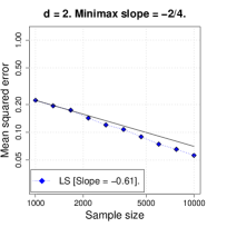
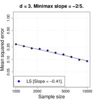
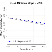
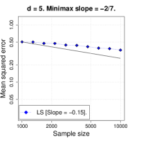
Figure 1: Mean squared error of Laplacian smoothing (LS) as a function of sample size $n$. Each plot is on the log-log scale, and the results are averaged over 5 repetitions, with Laplacian smoothing tuned for optimal average mean squared error. The black line shows the minimax rate (in slope only; the intercept is chosen to match the observed error).

Testing Error of Laplacian Smoothing.

For a given $0<\alpha<1$, define a threshold $\widehat{t}_{\alpha}$ as

$$\widehat{t}_{\alpha}=\frac{1}{n}\sum_{k=1}^{n}\frac{1}{(\rho\lambda_{k}+1)^{2}}+\frac{1}{n}\sqrt{\frac{2}{\alpha}\sum_{k=1}^{n}\frac{1}{(\rho\lambda_{k}+1)^{4}}},$$

where we recall $\lambda_{k}$ is the $k$th smallest eigenvalue of $L$. The Laplacian smoothing test is then simply

$$\widehat{\varphi}=\mathbf{1}\bigl{\{}\widehat{T}>\widehat{t}_{\alpha}\bigr{\}}.$$

We show in Appendix B that $\widehat{f}$ is a level-$\alpha$ test. In the next theorem, we upper bound the worst-case risk $R_{n}(\widehat{\varphi},H^{1}(\mathcal{X},M),\epsilon)$ of $\widehat{\varphi}$, whenever $\epsilon$ is at least (a constant times) the critical radius given in (10). For this to hold, we will require a tighter range of scalings for the graph radius $r$.

1. For constants $C_{0},c_{0}>0$, the neighborhood graph radius $r$ satisfies

   $$C_{0}\biggl{(}\frac{\log n}{n}\biggr{)}^{\frac{1}{d}}\leq r\leq c_{0}\wedge M^{\frac{(d-8)}{8+2d}}n^{\frac{d-20}{32+8d}}.$$

We will also require that the radius of the Sobolev class not be too large. Precisely, we will require $M\leq M_{\max}(d)$, where we define

$$M_{\max}(d):=\begin{cases*}n^{1/8}&{$d=1$}\\ n^{(4-d)/(4d)}&{$d\geq 2$}.\end{cases*}$$

We now give Theorem 3, our main testing result.

Theorem 3.

Given i.i.d. draws $(X_{i},Y_{i})$, $i=1,\ldots,n$ from (1), assume $f_{0}\in H^{1}(\mathcal{X},M)$ where $\mathcal{X}\subseteq\mathbb{R}^{d}$ with $d<4$, and $M\leq M_{\max}(d)$. Assume (P1), (P2) on the design distribution $P$, and assume $G_{n,r}$ is computed with a kernel $K$ satisfying (K1). There exist constants $N,C,C_{1},c_{1}>0$ such that for any $n\geq N$, and any radius $r$ as in (R2), the Laplacian smoothing test $\widehat{\varphi}$ based on the estimator $\widehat{f}$ in (2), with $\rho=(nr^{d+2})^{-1}n^{-4/(4+d)}M^{-8/(4+d)}$, satisfies the following: for any $b\geq 1$, if

$$\epsilon^{2}\geq CM^{2d/(4+d)}n^{-4/(4+d)}\biggl{(}b^{2}+b\sqrt{\frac{1}{\alpha}}\biggr{)},$$ (11)

then the worst-case risk satisfies the upper bound: $R_{n}(\widehat{\varphi},H^{1}(\mathcal{X},M),\epsilon)\leq C/b+C_{1}n\exp(-c_{1}nr^{d})\bigr{)}$.

Some remarks:

• As mentioned earlier, Sobolev balls $H^{1}(\mathcal{X},M)$ for $d\geq 4$ include quite irregular functions $f\not\in L^{4}(\mathcal{X})$. Proving tight lower bounds in this case is nontrivial, and as far as we understand such an analysis remains outstanding. On the other hand, if we explicitly assume that $f_{0}\in L^{4}(\mathcal{X},M)$, then Guerre and Lavergne (2002) show that the testing problem is characterized by a dimension-free lower bound $\epsilon^{2}(L^{4}(\mathcal{X},M))\gtrsim n^{-1/2}$. Moreover, by setting $\rho=0$ so that the resulting estimator $\widehat{f}$ interpolates the responses $Y_{1},\ldots,Y_{n}$, the subsequent test $\widehat{\varphi}$ will achieve (up to constants) this lower bound. That is, for any $f_{0}\in L^{4}(\mathcal{X},M)$ such that $\|f_{0}\|_{L^{2}(\mathcal{X})}^{2}\geq C(b^{2}+\sqrt{1/\alpha})n^{-1/2}$, we have that $\mathbb{E}_{0}[\widehat{\varphi}]\leq\alpha$ and

  $$\mathbb{E}_{f_{0}}\bigl{[}1-\widehat{\varphi}\bigr{]}\leq\frac{C(1+M^{4})}{b^{2}}.$$ (12)

• To compute the data-dependent threshold $\widehat{t}_{\alpha}$, one must know all of the eigenvalues $\lambda_{1},\ldots,\lambda_{n}$. Computing all these eigenvalues is far more expensive (cubic-time) than computing $\widehat{T}$ in the first place (nearly-linear-time). But in practice we would not recommend using $\widehat{t}_{\alpha}$ anyway, and would instead we make the standard recommendation to calibrate via a permutation test (Hoeffding, 1952). Recent work Kim et al. (2020), has shown that in a variety of closely related settings, calibration of a test statistic via the permutation test often retains minimax-optimal power, and we expect similar results to hold for the Laplacian smoothing-based test statistic.

More Discussion of Variational Analog.

With some results in hand, let us pause to offer some explanation of why Laplacian smoothing can be optimal in settings where thin-plate splines are not even consistent. First, we elaborate on why this difference in performance is so surprising. As mentioned previously, the penalties in (2), (4) can be closely tied together: Bousquet et al. (2004) show that for $f\in C^{2}(\mathcal{X})$,

$$\lim\frac{1}{n^{2}r^{d+2}}f^{\top}Lf =\int_{\mathcal{X}}f(x)\cdot\Delta_{P}f(x)p(x)\,dx$$ (13)

$$=\int_{\mathcal{X}}\|\nabla f(x)\|_{2}^{2}p^{2}(x)\,dx.$$

In the above, the limit is as $n\to\infty$ and $r\to 0$, $\Delta_{P}$ is the (weighted) Laplace-Beltrami operator

$$\Delta_{P}f:=-\frac{1}{p}\mathrm{div}\bigl{(}p^{2}\nabla f),$$

and the second equality follows using integration by parts. To be clear, this argument does not formally imply that the Laplacian eigenmaps estimator $\widehat{f}$ and the thin-plate spline estimator $\widetilde{f}$ are close (for one, note that (13) holds for $f\in C^{2}(\mathcal{X})$, whereas the optimization in (4) considers a much broader set of continuous functions with weak derivatives in $L^{2}(\mathcal{X})$). But it does seem to suggest that the two estimators should behave somewhat similarly.

Of course, we know this is not the case: $\widehat{f}$ and $\widetilde{f}$ look very different when $d>1$. What is driving this difference? The key point is that the discretization imposed by the graph $G_{n,r}$—which might seem problematic at first glance—turns out to be a blessing. The problem with (4) is that the class $H^{1}(\mathcal{X})$, which fundamentally underlies the criterion, is far “too big” for $d>1$. This is meant in various related senses. By the Sobolev embedding theorem, for $d>1$, the class $H^{1}(\mathcal{X})$ does not continuously embed into any Hölder space; and in fact it does not even continuously embed into $C^{0}(\mathcal{X})$. Thus we cannot really restrict the optimization to continuous and weakly differentiable functions, as we could when $d=1$ (the smoothing spline case), without throwing out a substantial subset of functions in $H^{1}(\mathcal{X})$. Even among continuous and differentiable functions $f$, as we explained previously, we can use “bump” functions (as in Green and Silverman (1993)) to construct $f$ that interpolates the pairs $(X_{i},Y_{i})$, $i=1,\ldots,n$ and achieves arbitrarily small penalty (and hence criterion) in (4). In this sense, any estimator resulting from solving (4) will clearly be inconsistent.

On the other hand, problem (2) is finite-dimensional. As a result $\widehat{f}$ has far less capacity to overfit than does $\widetilde{f}$, for any given sample size $n$. Discretization is not the only way to make the problem (4) more tractable: for instance, one can replace the penalty $\int_{\mathcal{X}}\|\nabla f(x)\|_{2}^{2}\,dx$ with a stricter choice like $\operatorname*{ess\,sup}_{x\in\mathcal{X}}\|\nabla f(x)\|_{2}$, or conduct the optimization over some finite-dimensional linear subspace of $H^{1}(\mathcal{X})$ (i.e., use a sieve). While these solutions do improve the statistical properties of $\widetilde{f}$ for $d>1$ (see e.g., Birgé and Massart (1993, 1998); van de Geer (2000)), Laplacian smoothing is generally speaking much simpler and more computationally friendly. In addition, the other approaches are usually specifically tailored to the domain $\mathcal{X}$, in stark contrast to $\widehat{f}$.

Overview of Analysis.

The comparison with thin-plate splines highlights some surprising differences between $\widehat{f}$ and $\widetilde{f}$. Such differences also preclude us from analyzing $\widehat{f}$ by, say, using (13) to establish a coupling between $\widehat{f}$ and $\widetilde{f}$—we know this cannot work, because we would like to prove meaningful error bounds on $\widehat{f}$ in regimes where no such bounds exist for $\widetilde{f}$.

Instead we take a different approach, and directly analyze the error of $\widehat{f}$ and $\widehat{T}$ using a bias-variance decomposition (conditional on $X_{1},\ldots,X_{n}$). A standard calculation shows that

$$\bigl{\|}\widehat{f}-f_{0}\bigr{\|}_{n}^{2}\leq\underbrace{\vphantom{\sum_{k=1}^{n}}\frac{2\rho}{n}\bigl{(}f_{0}^{\top}Lf_{0}\bigr{)}}_{\textrm{bias}}+\underbrace{\frac{10}{n}\sum_{k=1}^{n}\frac{1}{(\rho\lambda_{k}+1)^{2}}}_{\textrm{variance}},$$

and likewise that $\widehat{\varphi}$ has small risk whenever

$$\bigl{\|}f_{0}\bigr{\|}_{n}^{2}\geq\underbrace{\vphantom{\sqrt{\sum_{k=1}^{n}}}\frac{2\rho}{n}\bigl{(}f_{0}^{\top}Lf_{0}\bigr{)}}_{\textrm{bias}}+\underbrace{\frac{2\sqrt{2/\alpha}+2b}{n}\sqrt{\sum_{k=1}^{n}\frac{1}{(\rho\lambda_{k}+1)^{4}}}}_{\textrm{variance}}.$$

The bias and variance terms are each functions of the random graph $G_{n,r}$, and hence are themselves random. To upper bound them, we build on some recent works (Burago et al., 2014; García Trillos et al., 2019; Calder and García Trillos, 2019) regarding the consistency of neighborhood graphs to establish the following lemmas. These lemmas assume (P1), (P2) on the design distribution $P$, and (K1) on the kernel used to compute the neighborhood graph $G_{n,r}$.

Lemma 1.

There are constants $N,C_{2}>0$ such that for $n\geq N$, $r\leq c_{0}$, and $f\in H^{1}(\mathcal{X})$, with probability at least $1-\delta$, it holds that

$$f^{\top}Lf\leq\frac{C_{2}}{\delta}n^{2}r^{d+2}|f|_{H^{1}(\mathcal{X})}^{2}.$$ (14)

Lemma 2.

There are constants $N,C_{1},C_{3},c_{1},c_{3}>0$ such that for $n\geq N$ and $C_{0}(\log n/n)^{1/d}\leq r\leq c_{0}$, with probability at least $1-C_{1}n\exp(-c_{1}nr^{d})$, it holds that

$$c_{3}A_{n,r}(k)\leq\lambda_{k}\leq C_{3}A_{n,r}(k),~{}~{}\textrm{for $2\leq k\leq n$},$$ (15)

where $A_{n,r}(k)=\min\{nr^{d+2}k^{2/d},nr^{d}\}$.

Lemma 1 gives a direct upper bound on the bias term. Lemma 2 leads to a sufficiently tight upper bound on the variance term whenever the radius $r$ is sufficiently small; precisely, when $r$ is upper bounded as in (R1) for estimation, or (R2) for testing. The parameter $\rho$ is then chosen to minimize the sum of these upper bounds on bias and variance, as usual, and some straightforward calculations give Theorems 1-3.

It may be useful to give one more perspective on our approach. A common strategy in analyzing penalized least squares estimators is to assume two properties: first, that the regression function $f_{0}$ lies in (or near) a ball defined by the penalty operator; second, that this ball is reasonably small, e.g., as measured by metric entropy, or Rademacher complexity, etc. In contrast, in Laplacian smoothing, the penalty induces a ball

$$H^{1}(G_{n,r},M):=\{f:f^{\top}Lf\leq M^{2}\}$$

that is data-dependent and random, and so we do not have access to either of the aforementioned properties a priori, and instead, must prove they hold with high probability. In this sense, our analysis is different than the typical one in nonparametric regression.

5 Manifold Adaptivity

The minimax rates $n^{-2/(2+d)}$ and $n^{-4/(4+d)}$, in estimation and testing, suffer from the curse of dimensionality. However, in practice it can be often reasonable to assume a manifold hypothesis: that the data $X_{1},\ldots,X_{n}$ lie on a manifold $\mathcal{X}$ of $\mathbb{R}^{d}$ that has intrinsic dimension $m<d$. Under such an assumption, it is known (Bickel and Li, 2007; Arias-Castro et al., 2018) that the optimal rates over $H^{1}(\mathcal{X})$ are now $n^{-2/(2+m)}$ (for estimation) and $n^{-4/(4+m)}$ (for testing), which are much faster than the full-dimensional error rates when $m\ll d$.

On the other hand, a theory has been developed (Belkin, 2003; Belkin and Niyogi, 2008; Niyogi et al., 2008; Niyogi, 2013; Balakrishnan et al., 2012, 2013) establishing that the neighborhood graph $G_{n,r}$ can “learn” the manifold $\mathcal{X}$ in various senses, so long as $\mathcal{X}$ is locally linear. We contribute to this line of work by showing that under the manifold hypothesis, Laplacian smoothing achieves the tighter minimax rates over $H^{1}(\mathcal{X})$.

Error Rates Assuming the Manifold Hypothesis.

The conditions and results presented here will be largely similar to the previous ones, except with the ambient dimension $d$ replaced by the intrinsic dimension $m$. For the remainder, we assume the following.

1. $P$ is supported on a compact, connected, smooth manifold $\mathcal{X}$ embedded in $\mathbb{R}^{d}$, of dimension $m\leq d$. The manifold is without boundary and has positive reach (Federer, 1959).

2. $P$ admits a density $p$ with respect to the volume form of $\mathcal{X}$ such that

   $$0<p_{\min}\leq p(x)\leq p_{\max}<\infty,~{}~{}\textrm{for all $x\in\mathcal{X}$}.$$

   Additionally, $p$ is Lipschitz on $\mathcal{X}$, with Lipschitz constant $L_{p}$.

Under the assumptions (P3), (P4), and (K1), and for a suitable range of $r$, the error bounds on the estimator $\widehat{f}$ and test $\widehat{\varphi}$ will depend on $m$ instead of $d$.

1. For constants $C_{0},c_{0}>0$, the neighborhood graph radius $r$ satisfies

   $$C_{0}\biggl{(}\frac{\log n}{n}\biggr{)}^{\frac{1}{m}}\leq r\leq c_{0}\wedge M^{\frac{(m-4)}{(4+2m)}}n^{\frac{-3}{(4+2m)}}.$$

Theorem 4.

As in Theorem 1, but where $\mathcal{X}\subseteq\mathbb{R}^{d}$ is a manifold with intrinsic dimension $m<4$, the design distribution $P$ obeys (P3), (P4), and $M\leq n^{1/m}$. There are constants $N,C,c>0$ (not depending on $f_{0}$) such that for any $n\geq N$, and any $r$ as in (R4), the Laplacian smoothing estimator $\widehat{f}$ in (2), with $L=L_{n,r}$ and $\rho=M^{-4/(2+m)}(nr^{m+2})^{-1}n^{-2/(2+m)}$, satisfies

$$\bigl{\|}\widehat{f}-f_{0}\bigr{\|}_{n}^{2}\leq\frac{C}{\delta}M^{2m/(2+m)}n^{-2/(2+m)},$$

with probability at least $1-\delta-Cn\exp(-cnr^{m})-\exp(-c(M^{2}n)^{m/(2+m)})$.

In a similar vein, we obtain results for manifold adaptive testing under the following condition on the graph radius parameter.

1. For constants $C_{0},c_{0}>0$, the neighborhood graph radius $r$ satisfies

   $$C_{0}\biggl{(}\frac{\log n}{n}\biggr{)}^{\frac{1}{m}}\leq r\leq c_{0}\wedge M^{\frac{(m-8)}{8+2m}}n^{\frac{m-20}{32+8m}}.$$

Theorem 5.

As in Theorem 3, but where $\mathcal{X}\subseteq\mathbb{R}^{d}$ is a manifold with intrinsic dimension $m<4$, $M\leq M_{\max}(m)$, and the design distribution $P$ obeys (P3), (P4). There are constants $N,C,c>0$ such that for any $n\geq N$, and any $r$ as in (R5), the Laplacian smoothing test $\widehat{\varphi}$ based on the estimator $\widehat{f}$ in (2), with $\rho=(nr^{m+2})^{-1}n^{-4/(4+m)}M^{-8/(4+m)}$, satisfies the following: for any $b\geq 1$, if

$$\epsilon^{2}\geq CM^{2m/(4+m)}n^{-4/(4+m)}\biggl{(}b^{2}+b\sqrt{\frac{1}{\alpha}}\biggr{)},$$ (16)

then the worst-case risk satisfies the upper bound: $R_{n}(\widehat{\varphi},H^{1}(\mathcal{X},M),\epsilon)\leq C/b+Cn\exp(-cnr^{m})$.

The proofs of Theorems 4 and 5 proceed in a similar manner to that of Theorems 1 and 3. The key difference is that in the manifold setting, the equations (14) and (15) used to upper bound bias and variance will hold with $d$ replaced by $m$.

We emphasize that little about $\mathcal{X}$ need be known for Theorems 4 and 5 to hold. Indeed, all that is needed is the intrinsic dimension $m$, to properly tune $r$ and $\rho$ (from a theoretical point of view), and otherwise $\widehat{f}$ and $\widehat{\varphi}$ are computed without regard to $\mathcal{X}$. In contrast, the penalty in (4) would have to be specially tailored to work in this setting, revealing another advantage of the discrete approach over the variational one.

6 Discussion

We have shown that Laplacian smoothing, computed over a neighborhood graph, can be optimal for both estimation and goodness-of-fit testing over Sobolev spaces. There are many extensions worth pursuing, and several have already been mentioned. We conclude by mentioning a couple more. In practice, it is more common to use a $k$-nearest-neighbor (kNN) graph than a neighborhood graph, due to the guaranteed connectivity and sparsity of the former; we suspect that by building on the work of Calder and García Trillos (2019), one can show that our main results all hold under the kNN graph as well. In another direction, one can also generalize Laplacian smoothing by replacing the penalty $f^{\top}Lf$ with $f^{\top}L^{s}f$, for an integer $s>1$. The hope is that this would then achieve minimax optimal rates over the higher-order Sobolev class $H^{s}(\mathcal{X})$.

Acknowledgments

AG and RJT were supported by ONR grant N00014-20-1-2787. AG and SB were supported by NSF grants DMS-1713003 and CCF-1763734.

Appendix A Preliminaries

In the appendix, we provide complete proofs of all results. Our main theorems (Theorems 1-5) all follow the same general proof strategy of first establishing bounds in the fixed-design setup. In Section B, we establish (estimation or testing) error bounds which hold for any graph $G$; these bounds are stated with respect to (functionals of) the graph $G$, and allow us to upper bound the error of $\widehat{f}$ and $\widehat{\varphi}$ conditional on the design $\{X_{1},\ldots,X_{n}\}=\{x_{1},\ldots,x_{n}\}$. In Sections C, D, E, and F we develop all the necessary probabilistic estimates on these functionals, for the particular random neighborhood graph $G=G_{n,r}$. It is in these sections where we invoke our various assumptions on the distribution $P$ and regression function $f_{0}$. In Section G, we prove our main theorems and some other results. In Section H, we state a few concentration bounds that we use repeatedly in our proofs.

Pointwise evaluation of Sobolev functions.

First, however, as promised in our main text we clarify what is meant by pointwise evaluation of the regression function $f_{0}$. Strictly speaking, each $f\in H^{1}(X)$ is really an equivalence class, defined only up to sets of Lebesgue measure 0. In order to make sense of the evaluation $x\mapsto f(x)$, one must therefore pick a representative $f^{\star}\in f$. When $d=1$, this is resolved in a standard way—since $H^{1}(\mathcal{X})$ embeds continuously into $C^{0}(\mathcal{X})$, there exists a continuous version of every $f\in H^{1}(\mathcal{X})$, and we take this continuous version as the representative $f^{\star}$. On the other hand, when $d\geq 2$, the Sobolev space $H^{1}(\mathcal{X})$ does not continuously embed into $C^{0}(\mathcal{X})$, and we must choose representatives in a different manner. In this case we let $f^{\star}$ be the precise representative [Evans and Gariepy, 2015], defined pointwise at points $x\in\mathcal{X}$ as

$$f^{\star}(x)=\begin{dcases*}\lim_{\varepsilon\to 0}\frac{1}{\nu(B(x,\varepsilon))}\int_{B(x,\varepsilon)}f(z)dz,&~{}~{}{if the limit exists,}\\ 0,&~{}~{}{otherwise.}\end{dcases*}$$

Note that when $d=1$, the precise representative of any $f\in H^{1}(\mathcal{X})$ is continuous.

Now we explain why the particular choice of representative is not crucial, using the notion of a Lebesgue point. Recall that for a locally Lebesgue integrable function $f$, a given point $x\in\mathcal{X}$ is a Lebesgue point of $f$ if the limit of $1/(\nu(B(x,\varepsilon)))\int_{B(x,\varepsilon)}f(x)dx$ as $\varepsilon\to 0$ exists, and satisfies

$$\lim_{\varepsilon\to 0}\frac{1}{\nu\bigl{(}B(x,\varepsilon)\bigr{)}}\int_{B(x,\varepsilon)}f(x)dx=f(x).$$

Let $E$ denote the set of Lebesgue points of $f$. By the Lebesgue differentiation theorem [Evans and Gariepy, 2015], if $f\in L^{1}(\mathcal{X})$ then almost every $x\in\mathcal{X}$ is a Lebesgue point, $\nu(\mathcal{X}\setminus E)=0$. Since $f_{0}\in H^{1}(\mathcal{X})\subseteq L^{1}(\mathcal{X})$, we can conclude that any function $g_{0}\in f_{0}$ disagrees with the precise representative $f_{0}^{\star}$ only on a set of Lebesgue measure 0. Moreover, since we always assume the design distribution $P$ has a continuous density, with probability $1$ it holds that $g_{0}(X_{i})=f_{0}^{\star}(X_{i})$ for all $i=1,\ldots,n$. This justifies the notation $f_{0}(X_{i})$ used in the main text.

Appendix B Graph-dependent error bounds

In this section, we adopt the fixed design perspective; or equivalently, condition on $X_{i}=x_{i}$ for $i=1,\ldots,n$. Let $G=\bigl{(}[n],W\bigr{)}$ be a fixed graph on $\{1,\ldots,n\}$ with Laplacian matrix $L=D-W$. The randomness thus all comes from the responses

$$Y_{i}=f_{0}(x_{i})+\varepsilon_{i}$$ (17)

where the noise variables $\varepsilon_{i}$ are independent $N(0,1)$. In the rest of this section, we will mildly abuse notation and write $f_{0}=(f_{0}(x_{1}),\ldots,f_{0}(x_{n}))\in\mathbb{R}^{n}$. We will also write ${\bf Y}=(Y_{1},\ldots,Y_{n})$.

Recall (2) and (3): the Laplacian smoothing estimator of $f_{0}$ on $G$ is

$$\widehat{f}:=\operatorname*{argmin}_{f\in\mathbb{R}^{n}}\biggl{\{}\sum_{i=1}^{n}(Y_{i}-f_{i})^{2}+\rho\cdot f^{\top}Lf\biggr{\}}=(\rho L+I)^{-1}{\bf Y}.$$

and the Laplacian smoothing test statistic is

$$\widehat{T}:=\frac{1}{n}\|\widehat{f}\|_{2}^{2}.$$

We note that in this section, many of the derivations involved in upper bounding the estimation error of $\widehat{f}$ are similar to those of Sadhanala et al. [2016], with the difference being that we seek bounds in high probability rather than in expectation. We keep the work here self-contained for purposes of completeness.

B.1 Error bounds for linear smoothers

Let $S\in\mathbb{R}^{n\times n}$ be a fixed square, symmetric matrix, and let

$$\widecheck{f}:=SY$$

be a linear estimator of $f_{0}$. In Lemma 3 we upper bound the error $\frac{1}{n}\|\widecheck{f}-f_{0}\|_{2}^{2}$ as a function of the eigenvalues of $S$. Let $\bm{\lambda}(S)=(\lambda_{1}(S),\ldots,\lambda_{n}(S))\in\mathbb{R}^{n}$ denote these eigenvalues, and let $v_{k}(S)$ denote the corresponding unit-norm eigenvectors, so that $S=\sum_{k=1}^{n}\lambda_{k}(S)\cdot v_{k}(S)v_{k}(S)^{\top}$. Denote $Z_{k}=v_{k}(S)^{\top}\varepsilon$, and observe that ${\bf Z}=(Z_{1},\ldots,Z_{n})\sim N(0,I)$.

Lemma 3.

Let $\widecheck{f}=SY$ for a square, symmetric matrix, $S\in\mathbb{R}^{n\times n}$. Then

$$\mathbb{P}_{f_{0}}\biggl{(}\frac{1}{n}\bigl{\|}\widecheck{f}-f_{0}\bigr{\|}_{2}^{2}\geq\frac{10}{n}\bigl{\|}\bm{\lambda}(S)\bigr{\|}_{2}^{2}+\frac{2}{n}\bigl{\|}(S-I)f_{0}\bigr{\|}_{2}^{2}\biggr{)}\leq 1-\exp\Bigl{(}-\bigl{\|}\bm{\lambda}(S)\bigr{\|}_{2}^{2}\Bigr{)}$$

Here we have written $\mathbb{P}_{f_{0}}(\cdot)$ for the probability law under the regression “function” $f_{0}\in\mathbb{R}^{n}$.

In Lemma 4, we upper bound the error of a test involving the statistic $\|\widecheck{f}\|_{2}^{2}={\bf Y}^{\top}S^{2}{\bf Y}$. We will require that $S$ be a contraction, meaning that it has operator norm no greater than $1$, $\|Sv\|_{2}\leq\|v\|_{2}$ for all $v\in\mathbb{R}^{n}$.

Lemma 4.

Let $\widecheck{T}={\bf Y}^{\top}S^{2}{\bf Y}$ for a square, symmetric matrix $S\in\mathbb{R}^{n\times n}$. Suppose $S$ is a contraction. Define the threshold $\widecheck{t}_{\alpha}$ to be

$$\widecheck{t}_{\alpha}:=\lVert\bm{\lambda}(S)\rVert_{2}^{2}+\sqrt{\frac{2}{\alpha}}\lVert\bm{\lambda}(S)\rVert_{4}^{2}.$$ (18)

It holds that:

• Type I error.

  $$\mathbb{P}_{0}\bigl{(}\widecheck{T}>\widecheck{t}_{\alpha}\bigr{)}\leq\alpha.$$ (19)

• Type II error. Under the further assumption

  $$f_{0}^{\top}S^{2}f_{0}\geq\Bigl{(}2\sqrt{\frac{2}{\alpha}}+2b\Bigr{)}\cdot\lVert\bm{\lambda}(S)\rVert_{4}^{2},$$ (20)

  then

  $$\mathbb{P}_{f_{0}}\bigl{(}\widecheck{T}\leq\widecheck{t}_{\alpha}\bigr{)}\leq\frac{1}{b^{2}}+\frac{16}{b\lVert\bm{\lambda}(S)\rVert_{4}^{2}}.$$ (21)

Proof of Lemma 3.

The expectation $\mathbb{E}_{f_{0}}[\widecheck{f}]=Sf_{0}$, and by the triangle inequality,

$$\frac{1}{n}\bigl{\|}\widecheck{f}-f_{0}\bigr{\|}_{2}^{2} \leq\frac{2}{n}\Bigl{(}\bigl{\|}\widecheck{f}-\mathbb{E}_{f_{0}}[\widecheck{f}]\bigr{\|}_{2}^{2}+\bigl{\|}\mathbb{E}_{f_{0}}[\widecheck{f}]-f_{0}\bigr{\|}_{2}^{2}\Bigr{)}$$

$$=\frac{2}{n}\Bigl{(}\bigl{\|}S\varepsilon\bigr{\|}_{2}^{2}+\bigl{\|}(S-I)f_{0}\bigr{\|}_{2}^{2}\Bigr{)}.$$

Writing $\lVert S\varepsilon\rVert_{2}^{2}=\sum_{k=1}^{n}\lambda_{k}(S)^{2}Z_{k}^{2}$, the claim follows from the result of Laurent and Massart [2000] on concentration of $\chi^{2}$-random variables, which for completeness we restate in Lemma 16. To be explicit, taking $t=\lVert\bm{\lambda}(S)\rVert_{2}^{2}$ in Lemma 16 completes the proof of Lemma 3.

Proof of Lemma 4.

We compute the mean and variance of $T$ as a function of $f_{0}$, then apply Chebyshev’s inequality.

Mean. We make use of the eigendecomposition $S=\sum_{k=1}^{n}\lambda_{k}(S)\cdot v_{k}(S)v_{k}(S)^{\top}$ to obtain

$$=f_{0}^{\top}S^{2}f_{0}+2f_{0}^{\top}S^{2}\varepsilon+\varepsilon^{\top}S^{2}\varepsilon$$ (22)

$$=f_{0}^{\top}S^{2}f_{0}+2f_{0}^{\top}S^{2}\varepsilon+\sum_{k=1}^{n}\bigl{(}\lambda_{k}(S)\bigr{)}^{2}(\varepsilon^{\top}v_{k}(S))^{2}$$

$$=f_{0}^{\top}S^{2}f_{0}+2f_{0}^{\top}S^{2}\varepsilon+\sum_{k=1}^{n}\bigl{(}\lambda_{k}(S)\bigr{)}^{2}Z_{k}^{2},$$

implying

$$\mathbb{E}_{f_{0}}\bigl{[}\widecheck{T}\bigr{]}=f_{0}^{\top}S^{2}f_{0}+\sum_{k=1}^{n}\bigl{(}\lambda_{k}(S)\bigr{)}^{2}.$$ (23)

Variance. We start from (22). Recalling that $\mathrm{Var}(Z_{k}^{2})=2$, it follows from the Cauchy-Schwarz inequality that

$$\mathrm{Var}_{f_{0}}\bigl{[}\widecheck{T}\bigr{]}\leq 8f_{0}^{\top}S^{4}f_{0}+4\sum_{k=1}^{n}\bigl{(}\lambda_{k}(S)\bigr{)}^{4}.$$ (24)

Bounding Type I and Type II error. The upper bound (19) on Type I error follows immediately from (23), (24), and Chebyshev’s inequality.

We now establish the upper bound (21) on Type II error. From assumption (20), we see that $f_{0}^{\top}S^{2}f_{0}^{\top}-\widecheck{t}_{\alpha}\leq 0$. As a result,

$$\mathbb{P}_{f_{0}}\Bigl{(}\widecheck{T}\leq\widecheck{t}_{\alpha}\Bigr{)} =\mathbb{P}_{f_{0}}\Bigl{(}\widecheck{T}-\mathbb{E}_{f_{0}}\bigl{[}\widecheck{T}\bigr{]}\leq\widecheck{t}_{\alpha}-\mathbb{E}_{f_{0}}\bigl{[}\widecheck{T}\bigr{]}\Bigr{)}$$

$$\leq\mathbb{P}_{f_{0}}\Bigl{(}\Bigl{|}\widecheck{T}-\mathbb{E}_{f_{0}}\bigl{[}\widecheck{T}\bigr{]}\Bigr{|}\geq\Bigl{|}\widecheck{t}_{\alpha}-\mathbb{E}_{f_{0}}\bigl{[}\widecheck{T}\bigr{]}\Bigr{|}\Bigr{)}$$

$$\leq\frac{\mathrm{Var}_{f_{0}}\bigl{[}\widecheck{T}\bigr{]}}{\bigl{(}\widecheck{t}_{\alpha}-\mathbb{E}_{f_{0}}\bigl{[}\widecheck{T}\bigr{]}\bigr{)}^{2}},$$

where the last line follows from Chebyshev’s inequality. Plugging in the expressions (23) and (24) for the mean and variance of $\widecheck{T}$, as well as the definition of $\widecheck{t}_{\alpha}$ in (18), we obtain that

$$\mathbb{P}_{f_{0}}\Bigl{(}\widecheck{T}\leq\widecheck{t}_{\alpha}\Bigr{)}\leq\frac{4\|\bm{\lambda}(S)\|_{4}^{4}}{\bigl{(}f_{0}^{\top}S^{2}f_{0}-\sqrt{2/\alpha}\lVert\bm{\lambda}(S)\rVert_{4}^{2}\bigr{)}^{2}}+\frac{8f_{0}^{\top}S^{4}f_{0}}{\bigl{(}f_{0}^{\top}S^{2}f_{0}-\sqrt{2/\alpha}\lVert\bm{\lambda}(S)\rVert_{4}^{2}\bigr{)}^{2}}.$$ (25)

We now use the assumed lower bound $f_{0}^{\top}S^{2}f_{0}\geq(2\sqrt{2/\alpha}+2b)\lVert\bm{\lambda}(S)\rVert_{4}^{2}$ to separately upper bound each of the two terms on the right hand side of (25). It follows immediately that

$$\frac{4\|\bm{\lambda}(S)\|_{4}^{4}}{\bigl{(}f_{0}^{\top}S^{2}f_{0}-\sqrt{2/\alpha}\lVert\bm{\lambda}(S)\rVert_{4}^{2}\bigr{)}^{2}}\leq\frac{1}{b^{2}},$$ (26)

giving a sufficient upper bound on the first term. Now we upper bound the second term,

$$\frac{8f_{0}^{\top}S^{4}f_{0}}{\bigl{(}f_{0}^{\top}S^{2}f_{0}-\sqrt{2/\alpha}\lVert\bm{\lambda}(S)\rVert_{4}^{2}\bigr{)}^{2}}\leq\frac{32f_{0}^{\top}S^{4}f_{0}}{\bigl{(}f_{0}^{\top}S^{2}f_{0}\bigr{)}^{2}}\leq\frac{16}{b\|\bm{\lambda}(S)\|_{4}^{2}}\frac{f_{0}^{\top}S^{4}f_{0}}{f_{0}^{\top}S^{2}f_{0}}\leq\frac{16}{b\|\bm{\lambda}(S)\|_{4}^{2}},$$ (27)

where the final inequality is satisfied because $S$ is a contraction. Plugging (26) and (27) back into (25) then gives the desired result.

B.2 Analysis of Laplacian smoothing

Upper bounds on the mean squared error of $\widehat{f}$, and Type I and Type II error of $\widehat{T}$, follow from setting $S=(\rho L+I)^{-1}$ in Lemmas 3 and 4. We give these results in Lemma 5 and 6, and prove them immediately. Recall that $\lambda_{1},\ldots,\lambda_{n}$ are the $n$ eigenvalues of $L$ (sorted in ascending order).

Lemma 5.

For any $\rho>0$,

$$\frac{1}{n}\bigl{\|}\widehat{f}-f_{0}\bigr{\|}_{2}^{2}\leq\frac{2\rho}{n}\bigl{(}f_{0}^{\top}Lf_{0}\bigr{)}+\frac{10}{n}\sum_{k=1}^{n}\frac{1}{\bigl{(}\rho\lambda_{k}+1\bigr{)}^{2}},$$ (28)

with probability at least $1-\exp\Bigl{(}-\sum_{k=1}^{n}\bigl{(}\rho\lambda_{k}+1\bigr{)}^{-2}\Bigr{)}$.

Recall that

$$\widehat{t}_{\alpha}:=\frac{1}{n}\sum_{k=1}^{n}\frac{1}{\bigl{(}\rho\lambda_{k}+1\bigr{)}^{2}}+\frac{1}{n}\sqrt{\frac{2}{\alpha}\sum_{k=1}^{n}\frac{1}{\bigl{(}\rho\lambda_{k}+1\bigr{)}^{4}}}.$$

Lemma 6.

For any $\rho>0$ and any $b\geq 1$, it holds that:

• Type I error.

  $$\mathbb{P}_{0}\Bigl{(}\widehat{T}>\widehat{t}_{\alpha}\Bigr{)}\leq\alpha.$$ (29)

• Type II error. If

  $$\frac{1}{n}\lVert f_{0}\rVert_{2}^{2}\geq\frac{2\rho}{n}\bigl{(}f_{0}^{\top}Lf_{0}\bigr{)}+\frac{2\sqrt{2/\alpha}+2b}{n}\Biggl{(}\sum_{k=1}^{n}\frac{1}{(\rho\lambda_{k}+1)^{4}}\Biggr{)}^{1/2},$$ (30)

  then

  $$\mathbb{P}_{f_{0}}\Bigl{(}\widehat{T}(G)\leq\widehat{t}_{\alpha}\Bigr{)}\leq\frac{1}{b^{2}}+\frac{16}{b}\Biggl{(}\sum_{k=1}^{n}\frac{1}{(\rho\lambda_{k}+1)^{4}}\Biggr{)}^{-1/2}.$$ (31)

Proof of Lemma 5.

Let $\widehat{S}=(I+\rho L)^{-1}$, the estimator $\widehat{f}=\widehat{S}Y$, and

$$\bigl{\|}\bm{\lambda}(\widehat{S})\bigr{\|}_{2}^{2}=\sum_{k=1}^{n}\frac{1}{\bigl{(}1+\rho\lambda_{k}\bigr{)}^{2}}.$$

We deduce the following upper bound on the bias term,

$$\bigl{\|}(\widehat{S}-I)f_{0}\bigr{\|}_{2}^{2} =f_{0}^{\top}L^{1/2}L^{-1/2}\bigl{(}\widehat{S}-I\bigr{)}^{2}L^{-1/2}L^{1/2}f_{0}$$

$$\leq f_{0}^{\top}Lf_{0}\cdot\lambda_{n}\Bigl{(}L^{-1/2}\bigl{(}\widehat{S}-I\bigr{)}^{2}L^{-1/2}\Bigr{)}$$

$$=f_{0}^{\top}Lf_{0}\cdot\max_{k\in[n]}\biggl{\{}\frac{1}{\lambda_{k}}\Bigl{(}1-\frac{1}{\rho\lambda_{k}+1}\Bigr{)}^{2}\biggr{\}}$$

$$\leq f_{0}^{\top}Lf_{0}\cdot\rho.$$

In the above, we have written $L^{-1/2}$ for the square root of the pseudoinverse of $L$, the maximum is over all indices $k$ such that $\lambda_{k}>0$, and the last inequality follows from the basic algebraic identity $1-1/(1+x)^{2}\leq 2x$ for any $x>0$. The claim of the Lemma then follows from Lemma 3.

Proof of Lemma 6.

Let $\widehat{S}:=(I+\rho L)^{-1}$, so that $\widehat{T}=\frac{1}{n}{\bf Y}^{\top}\widehat{S}^{2}{\bf Y}$. Note that $\widehat{S}$ is a contraction, so that we may invoke Lemma 4. The bound on Type I error (29) follows immediately from (19). To establish the bound on Type II error, we must lower bound $f_{0}^{\top}\widehat{S}^{2}f_{0}$. We first note that by assumption (30),

$$f_{0}^{\top}\widehat{S}^{2}f_{0} =\bigl{\|}f_{0}\bigr{\|}_{2}^{2}-f_{0}^{\top}(I-\widehat{S}^{2})f_{0}$$

$$\geq 2\rho\bigl{(}f_{0}^{\top}Lf_{0}\bigr{)}-f_{0}^{\top}\bigl{(}I-\widehat{S}^{2}\bigr{)}f_{0}+\Bigl{(}2\sqrt{\frac{2}{\alpha}}+2b\Bigr{)}\cdot\Biggl{(}\sum_{k=1}^{n}\frac{1}{(\rho\lambda_{k}+1)^{4}}\Biggr{)}^{-1/2}.$$

Upper bounding $f_{0}^{\top}\bigl{(}I-\widehat{S}^{2}\bigr{)}f_{0}$ as follows:

$$f_{0}^{\top}\Bigl{(}I-\widehat{S}^{2}\Bigr{)}f_{0} =f_{0}^{\top}L^{1/2}L^{-1/2}\Bigl{(}I-\widehat{S}^{2}\Bigr{)}L^{-1/2}L^{1/2}f_{0}$$

$$\leq f_{0}^{\top}Lf_{0}\cdot\lambda_{n}\biggl{(}L^{-1/2}\Bigl{(}I-\widehat{S}^{2}\Bigr{)}L^{-1/2}\biggr{)}$$

$$=f_{0}^{\top}Lf_{0}\cdot\max_{k}\biggl{\{}\frac{1}{\lambda_{k}}\Bigl{(}1-\frac{1}{(\rho\lambda_{k}+1)^{2}}\Bigr{)}\biggr{\}}$$

$$\leq f_{0}^{\top}Lf_{0}\cdot 2\rho,$$

—where in the above the maximum is over all indices $k$ such that $\lambda_{k}>0$—we deduce that

$$f_{0}^{\top}\widehat{S}^{2}f_{0}\geq\Bigl{(}2\sqrt{\frac{2}{\alpha}}+2b\Bigr{)}\cdot\biggl{(}\sum_{k=1}^{n}\frac{1}{(\rho\lambda_{k}+1)^{4}}\biggr{)}^{-1/2}.$$

The upper bound on Type II error (31) then follows from Lemma 4.

Appendix C Neighborhood graph Sobolev semi-norm

In this section, we prove Lemma 1, which states an upper bound on $f^{\top}Lf$ that holds when $f$ is bounded in Sobolev norm. We also establish stronger bounds in the case when $f$ has a bounded Lipschitz constant; this latter result justifies one of our remarks after Theorem 1.

Throughout this proof, we will assume that $f\in H^{1}(\mathcal{X})$ has zero-mean, meaning $\int_{\mathcal{X}}f(x)\,dx=0$. This is without loss of generality—assuming for the moment that (14) holds for zero-mean functions, for any $f\in H^{1}(\mathcal{X})$, taking $a=\int_{\mathcal{X}}f(x)\,dx$ and $g=f-a$, we have that

$$f^{\top}Lf=g^{\top}Lg\leq\frac{C_{2}}{\delta}n^{2}r^{d+2}|g|_{H^{1}(\mathcal{X})}^{2}=\frac{C_{2}}{\delta}n^{2}r^{d+2}|f|_{H^{1}(\mathcal{X})}^{2}.$$

Now, for any zero-mean function $f\in H^{1}(\mathcal{X})$ it follows by the Poincare inequality (see Section 5.8, Theorem 1 of Evans [2010]) that $\|f\|_{H^{1}(\mathcal{X})}^{2}\leq C_{8}|f|_{H^{1}(\mathcal{X})}^{2}$, for some constant $C_{8}$ that does not depend on $f$. Therefore, to prove Lemma 1, it suffices to show that

$$\mathbb{E}\Bigl{[}f^{\top}Lf\Bigr{]}\leq Cn^{2}r^{d+2}\|f\|_{H^{1}(\mathcal{X})}^{2},$$

since the high-probability upper bound then follows immediately by Markov’s inequality. (Recall that $L$ is positive semi-definite, and therefore $f^{\top}Lf$ is a non-negative random variable).

Since

$$f^{\top}Lf=\frac{1}{2}\sum_{i,j=1}^{n}\bigl{(}f(X_{i})-f(X_{j})\bigr{)}^{2}W_{ij},$$

it follows that

$$\mathbb{E}\Bigl{[}f^{\top}Lf\Bigr{]}=\frac{n(n-1)}{2}\mathbb{E}\biggl{[}\Bigl{(}f(X^{\prime})-f(X)\Bigr{)}^{2}K\biggl{(}\frac{\|X^{\prime}-X\|}{r}\biggr{)}\biggr{]},$$ (32)

where $X$ and $X^{\prime}$ are random variables independently drawn from $P$.

Now, take $\Omega$ to be an arbitrary bounded open set such that $B(x,c_{0})\subseteq\Omega$ for all $x\in\mathcal{X}$. For the remainder of this proof, we will assume that (i) $f\in H^{1}(\Omega)$ and additionally (ii) $\|f\|_{H^{1}(\Omega)}\leq C_{5}\|f\|_{H^{1}(\mathcal{X})}$ for a constant $C_{5}$ that does not depend on $f$. This is without loss of generality, since by Theorem 1 in Chapter 5.4 of Evans [2010] there exists an extension operator $E:H^{1}(\mathcal{X})\to H^{1}(\Omega)$ for which the extension $Ef$ satisfies both (i) and (ii). Additionally, we will assume $f\in C^{\infty}(\Omega)$. Again, this is without loss of generality, as $C^{\infty}(\Omega)$ is dense in $H^{1}(\Omega)$ and the expectation on the right hand side of (32) is continuous in $H^{1}(\Omega)$. The reason for dealing with a smooth extension $f\in C^{\infty}(\Omega)$ is so that we can make sense of the following equality for any $x$ and $x^{\prime}$ in $\mathcal{X}$:

$$f(x^{\prime})-f(x)=\int_{0}^{1}\nabla f\bigl{(}x+t(x^{\prime}-x)\bigr{)}^{\top}(x^{\prime}-x)\,dt.$$ (33)

Obviously

$$\mathbb{E}\biggl{[}\bigl{(}f(X^{\prime})-f(X)\bigr{)}^{2}K\biggl{(}\frac{\|X^{\prime}-X\|}{r}\biggr{)}\biggr{]}\leq p_{\max}^{2}\int_{\mathcal{X}}\int_{\mathcal{X}}\bigl{(}f(x^{\prime})-f(x)\bigr{)}^{2}K\biggl{(}\frac{\|x^{\prime}-x\|}{r}\biggr{)}\,dx^{\prime}\,dx,$$ (34)

so that it remains now to bound the double integral. Replacing difference by integrated derivative as in (33), we obtain

$$\int_{\mathcal{X}}\int_{\mathcal{X}}\bigl{(}f(x^{\prime})-f(x)\bigr{)}^{2}K\biggl{(}\frac{\|x^{\prime}-x\|}{r}\biggr{)}\,dx^{\prime}\,dx =\int_{\mathcal{X}}\int_{\mathcal{X}}\biggl{[}\int_{0}^{1}\nabla f\bigl{(}x+t(x^{\prime}-x)\bigr{)}^{\top}(x^{\prime}-x)\,dt\biggr{]}^{2}K\biggl{(}\frac{\|x^{\prime}-x\|}{r}\biggr{)}\,dx^{\prime}\,dx$$

$$\overset{(i)}{\leq}\int_{\mathcal{X}}\int_{\mathcal{X}}\int_{0}^{1}\biggl{[}\nabla f\bigl{(}x+t(x^{\prime}-x)\bigr{)}^{\top}(x^{\prime}-x)\biggr{]}^{2}K\biggl{(}\frac{\|x^{\prime}-x\|}{r}\biggr{)}\,dt\,dx^{\prime}\,dx$$

$$\overset{(ii)}{\leq}r^{d+2}\int_{\mathcal{X}}\int_{B(0,1)}\int_{0}^{1}\biggl{[}\nabla f\bigl{(}x+trz\bigr{)}^{\top}z\biggr{]}^{2}K\bigl{(}\|z\|\bigr{)}\,dt\,dz\,dx$$

$$\overset{(iii)}{\leq}r^{d+2}\int_{\Omega}\int_{B(0,1)}\int_{0}^{1}\Bigl{[}\nabla f\bigl{(}\widetilde{x}\bigr{)}^{\top}z\Bigr{]}^{2}K\bigl{(}\|z\|\bigr{)}\,dt\,dz\,d\widetilde{x},$$ (35)

where $(i)$ follows by Jensen’s inequality, $(ii)$ follows by substituting $z=(x^{\prime}-x)/r$ and (K1), and $(iii)$ by exchanging integrals, substituting $\widetilde{x}=x+trz$, and noting that $x\in\mathcal{X}$ implies that $\widetilde{x}\in\Omega$.

Now, writing $\bigl{(}\nabla f(\widetilde{x})^{\top}z\bigr{)}^{2}=\bigl{(}\sum_{i=1}^{d}z_{i}f^{(e_{i})}(x)\bigr{)}^{2}$, expanding the square and integrating, we have that for any $\widetilde{x}\in\mathcal{X}$,

$$\int_{B(0,1)}\Bigl{[}\nabla f\bigl{(}\widetilde{x}\bigr{)}^{\top}z\Bigr{]}^{2}K\bigl{(}\|z\|\bigr{)}\,dz =\sum_{i,j=1}^{d}f^{(e_{i})}(\widetilde{x})f^{(e_{j})}(\widetilde{x})\int_{\mathbb{R}^{d}}z_{i}z_{j}K(\|z\|)\,dz$$

$$=\sum_{i=1}^{d}\bigl{(}f^{(e_{i})}(\widetilde{x})\bigr{)}^{2}\int_{B(0,1)}z_{i}^{2}K\bigl{(}\|z\|\bigr{)}\,dz$$

$$=\sigma_{K}\|\nabla f(\widetilde{x})\|^{2},$$

where the last equality follows from the rotational symmetry of $K(\|z\|)$. Plugging back into (35), we obtain

$$\int_{\mathcal{X}}\int_{\mathcal{X}}\bigl{(}f(x^{\prime})-f(x)\bigr{)}^{2}K\biggl{(}\frac{\|x^{\prime}-x\|}{r}\biggr{)}\,dx^{\prime}\,dx\leq r^{d+2}\sigma_{K}\|f\|_{H^{1}(\Omega)}^{2}\leq C_{5}r^{d+2}\sigma_{K}\|f\|_{H^{1}(\mathcal{X})}^{2},$$

proving the claim of Lemma 1 upon taking $C_{2}:=C_{8}C_{5}\sigma_{K}p_{\max}^{2}$ in the statement of the lemma.

C.1 Stronger bounds under Lipschitz assumption

Suppose $f$ satisfies $|f(x^{\prime})-f(x)|\leq M\|x-x\|$ for all $x,x^{\prime}\in\mathcal{X}$. Then we can strengthen the high probability bound in Lemma 1 from $1-\delta$ to $1-\delta^{2}/n$, at the cost of only a constant factor in the upper bound on $f^{\top}Lf$.

Proposition 1.

Let $r\geq C_{0}(\log n/n)^{1/d}$. For any $f$ such that $|f(x^{\prime})-f(x)|\leq M\|x-x\|$ for all $x,x^{\prime}\in\mathcal{X}$, with probability at least $1-C\delta^{2}/n$ it holds that

$$f^{\top}Lf\leq\biggl{(}\frac{1}{\delta}+C_{2}\biggr{)}n^{2}r^{d+2}M^{2}.$$

Proof of Proposition 1.

We will prove Proposition 1 using Chebyshev’s inequality, so the key step is to upper bound the variance of $f^{\top}Lf$. Putting $\varDelta_{ij}:=K(\|X_{i}-X_{j}\|/r)\cdot(f(X_{i})-f(X_{j}))^{2}$, we can write the variance of $f^{\top}Lf$ as a sum of covariances,

$$\mathrm{Var}\bigl{[}f^{\top}Lf\bigr{]}=\frac{1}{4}\sum_{i,j=1}^{n}\sum_{\ell,m=1}^{n}\mathrm{Cov}\bigl{[}\varDelta_{ij},\varDelta_{\ell m}\bigr{]}.$$

Clearly $\mathrm{Cov}\bigl{[}\varDelta_{ij},\varDelta_{\ell m}\bigr{]}$ depends on the cardinality of $I:=\{i,j,k,\ell\}$; we divide into cases, and upper bound the covariance in each case.

1. In this case $\varDelta_{ij}$ and $\varDelta_{\ell m}$ are independent, and $\mathrm{Cov}\bigl{[}\varDelta_{ij},\varDelta_{\ell m}\bigr{]}=0$.

2. Taking $i=\ell$ without loss of generality, and noting that the expectation of $\Delta_{ij}$ and $\Delta_{im}$ is non-negative, we have

   $$\mathrm{Cov}\bigl{[}\varDelta_{ij},\varDelta_{im}\bigr{]} \leq\mathbb{E}\bigl{[}\varDelta_{ij}\varDelta_{im}\bigr{]}$$

   $$=\int_{\mathcal{X}}\int_{\mathcal{X}}\int_{\mathcal{X}}\bigl{(}f(z)-f(x)\bigr{)}^{2}\bigl{(}f(x^{\prime})-f(x)\bigr{)}^{2}K\biggl{(}\frac{\|x^{\prime}-x\|}{r}\biggr{)}K\biggl{(}\frac{\|z-x\|}{r}\biggr{)}p(z)p(x^{\prime})p(x)\,dz\,dx^{\prime}\,dx$$

   $$\leq p_{\max}^{3}M^{4}r^{4}\int_{\mathcal{X}}\int_{\mathcal{X}}\int_{\mathcal{X}}K\biggl{(}\frac{\|x^{\prime}-x\|}{r}\biggr{)}K\biggl{(}\frac{\|z-x\|}{r}\biggr{)}\,dz\,dx^{\prime}\,dx$$

   $$\leq p_{\max}^{3}M^{4}r^{4+2d}.$$

3. Taking $i=\ell$ and $j=m$ without loss of generality, we have

   $$\mathrm{Var}\bigl{[}\varDelta_{ij}\bigr{]} \leq\mathbb{E}\bigl{[}\varDelta_{ij}^{2}\bigr{]}$$

   $$\leq\int_{\mathcal{X}}\int_{\mathcal{X}}\bigl{(}f(x^{\prime})-f(x)\bigr{)}^{4}\biggl{[}K\biggl{(}\frac{\|x^{\prime}-x\|}{r}\biggr{)}\biggr{]}^{2}p(x^{\prime})p(x)\,dx^{\prime}\,dx$$

   $$\leq p_{\max}^{2}M^{4}r^{4}K(0)\int_{\mathcal{X}}\int_{\mathcal{X}}K\biggl{(}\frac{\|x^{\prime}-x\|}{r}\biggr{)}\,dx^{\prime}\,dx$$

   $$\leq p_{\max}^{2}M^{4}r^{4+d}K(0).$$

4. In this case $\varDelta_{ij}=\varDelta_{\ell m}=0$.

Therefore

$$\mathrm{Var}\bigl{[}f^{\top}Lf\bigr{]}\leq n^{3}p_{\max}^{3}M^{4}r^{4+2d}+n^{2}p_{\max}^{2}M^{4}r^{4+d}K(0)\leq CM^{4}n^{3}r^{4+2d},$$

where the latter inequality follows since $nr^{d}\gg 1$. For any $\delta>0$, it follows from Chebyshev’s inequality that

$$\mathbb{P}\biggl{(}\Bigl{|}f^{\top}Lf-\mathbb{E}\bigl{[}f^{\top}Lf\bigr{]}\Bigr{|}\geq\frac{M^{2}}{\delta}n^{2}r^{d+2}\biggr{)}\leq C\frac{\delta^{2}}{n},$$

and since we have already upper bounded $\mathbb{E}\bigl{[}f^{\top}Lf\bigr{]}\leq C_{2}M^{2}n^{2}r^{d+2}$, the proposition follows.

Note that the bound on $\mathrm{Var}[\varDelta_{ij}]$ follows as long as we can control $\|\nabla f\|_{L^{4}(\mathcal{X})}$; this implies the Lipschitz assumption—which gives us control of $\|\nabla f\|_{L^{\infty}(\mathcal{X})}$—can be weakened. However, the Sobolev assumption—which gives us control only over $\|\nabla f\|_{L^{2}(\mathcal{X})}$—will not do the job.

Appendix D Bounds on neighborhood graph eigenvalues

In this section, we prove Lemma 2, following the lead of Burago et al. [2014], García Trillos et al. [2019], Calder and García Trillos [2019], who establish similar results with respect to a manifold without boundary. To prove this lemma, in Theorem 6 we give estimates on the difference between eigenvalues of the graph Laplacian $L$ and eigenvalues of the weighted Laplace-Beltrami operator $\Delta_{P}$. We recall $\Delta_{P}$ is defined as

$$\Delta_{P}f(x):=-\frac{1}{p(x)}\mathrm{div}\bigl{(}p^{2}\nabla f\bigr{)}(x).$$

To avoid confusion, in this section we write $\lambda_{k}(G_{n,r})$ for the $k$th smallest eigenvalue of the graph Laplacian matrix $L$ and $\lambda_{k}(\Delta_{P})$ for the $k$th smallest eigenvalue of $\Delta_{P}$ . Some other notation: throughout this section, we will write $A,A_{0},A_{1},\ldots$ and $a,a_{0},a_{1},\ldots$ for constants which may depend on $\mathcal{X}$, $d$, $K$, and $p$, but do not depend on $n$; we keep track of all such constants explicitly in our proofs. We let $L_{K}$ denote the Lipschitz constant of the kernel $K$. Finally, for notational ease we set $\theta$ and $\widetilde{\delta}$ to be the following (small) positive numbers:

$$\widetilde{\delta}:=\max\Biggl{\{}n^{-1/d},\min\biggl{\{}\frac{1}{2^{d+3}A_{0}},\frac{1}{A_{3}},\frac{K(1)}{8L_{K}A_{0}},\frac{1}{8\max\{A_{1},A\}c_{0}}\biggr{\}}r\Biggr{\}},~{}~{}\textrm{and}~{}~{}\theta:=\frac{1}{8\max\{A_{1},A\}}.$$ (36)

We note that each of $\widetilde{\delta},\theta$ and $\widetilde{\delta}/r$ are of at most constant order.

Theorem 6.

For any $\ell\in\mathbb{N}$ such that

$$1-A\Biggl{(}r\sqrt{\lambda_{\ell}(\Delta_{P})}+\theta+\widetilde{\delta}\Biggr{)}\geq\frac{1}{2}$$ (37)

with probability at least $1-A_{0}n\exp(-a_{0}n\theta^{2}\widetilde{\delta}^{d})$, it holds that

$$a\lambda_{k}(G_{n,r})\leq nr^{d+2}\lambda_{k}(\Delta_{P})\leq A\lambda_{k}(G_{n,r}),~{}~{}\textrm{for all $1\leq k\leq\ell$}$$ (38)

Before moving forward to the proofs of Lemma 2 and Theorem 6, it is worth being clear about the differences between Theorem 6 and the results of Burago et al. [2014], García Trillos et al. [2019], Calder and García Trillos [2019]. First of all, the reason we cannot directly use the results of these works in the proof of Lemma 2 is that they all assume the domain $\mathcal{X}$ is without boundary, whereas for our results in Section 4 we instead assume $\mathcal{X}$ has a (Lipschitz smooth) boundary. Fortunately, in this setting the high-level strategy shared by Burago et al. [2014], García Trillos et al. [2019], Calder and García Trillos [2019] can still be used—indeed we follow it closely, as we summarize in Section D.1. However, many calculations need to be redone, in order to account for points $x$ which are on or sufficiently close to the boundary of $\mathcal{X}$. For completeness and ease of reading, we provide a self-contained proof of Theorem 6, but we comment where appropriate on connections between the technical results we use in this proof, and those derived in Burago et al. [2014], García Trillos et al. [2019], Calder and García Trillos [2019].

On the other hand, we should also point out that unlike the results of Burago et al. [2014], García Trillos et al. [2019], Calder and García Trillos [2019], Theorem 6 does not imply that $\lambda_{k}(G_{n,r})$ is a consistent estimate of $\lambda_{k}(\Delta_{P})$, i.e. it does not imply that $|(nr^{d+2})^{-1}\lambda_{k}(G_{n,r})-\lambda_{k}(\Delta_{P})|\to 0$ as $n\to\infty,r\to 0$. The key difficulty in proving consistency when $\mathcal{X}$ has a boundary can be summarized as follows: while at points $x\in\mathcal{X}$ satisfying $B(x,r)\subseteq\mathcal{X}$, the graph Laplacian $L$ is a reasonable approximation of the operator $\Delta_{P}$, at points $x$ near the boundary $L$ is known to approximate a different operator altogether [Belkin et al., 2012]. This is reminiscent of the boundary effects present in the analysis of kernel smoothing. We believe a more subtle analysis might imply convergence of eigenvalues in this setting. However, the conclusion of Theorem 6—that $\lambda_{k}(G_{n,r})/(nr^{d+2}\lambda_{k}(\Delta_{P}))$ is bounded above and below by constants that do not depend on $k$—suffices for our purposes.

The bulk of the remainder of this section is devoted to the proof of Theorem 6. First, however, we show that under our regularity conditions on $p$ and $\mathcal{X}$, Lemma 2 is a simple consequence of Theorem 6. The link between the two is Weyl’s Law.

Proposition 2 (Weyl’s Law).

Suppose the density $p$ and the domain $\mathcal{X}$ satisfy (P1) and (P2). Then there exist constants $a_{2}$ and $A_{2}$ such that

$$a_{2}k^{2/d}\leq\lambda_{k}(\Delta_{P})\leq A_{2}k^{2/d}~{}~{}\textrm{for all $k\in\mathbb{N},k>1$}.$$ (39)

See Lemma 28 of Dunlop et al. [2020] for a proof that (P1) and (P2) imply Weyl’s Law.

Proof of Lemma 2.

Put

$$\ell_{\star}=\left\lfloor\biggl{(}\frac{\bigl{(}1/(2A)-(\theta+\widetilde{\delta})\bigr{)}}{rA_{2}^{1/2}}\biggr{)}^{d}\right\rfloor.$$

Let us verify that $\lambda_{\ell_{\star}}(\Delta_{P})$ satisfies the condition (37) of Theorem 6. Setting $c_{0}:=1/(2^{1/d}4A_{2}^{1/2})$, the assumed upper bound on the radius $r\leq c_{0}$ guarantees that $\ell_{\star}\geq 2$. Therefore, by Proposition 2 we have that

$$\sqrt{\lambda_{\ell_{\star}}(\Delta_{P})}\leq A_{2}^{1/2}\ell_{\star}^{1/d}\leq\frac{1}{r}\biggl{(}\frac{1}{2A}-(\theta+\widetilde{\delta})\biggr{)}.$$

Rearranging the above inequality shows that condition (37) is satisfied.

It is therefore the case that the inequalities in (38) hold with probability at least $1-A_{0}n\exp(-a_{0}n\theta^{2}\widetilde{\delta}^{d})$. Together, (38) and (39) imply the following bounds on the graph Laplacian eigenvalues:

$$\frac{a}{A_{2}}nr^{d+2}k^{2/d}\leq\lambda_{k}(G_{n,r})\leq\frac{A}{a_{2}}nr^{d+2}k^{2/d}~{}~{}\textrm{for all $2\leq k\leq\ell_{\star}$}.$$

It remains to bound $\lambda_{k}(G_{n,r})$ for those indices $k$ which are greater than $\ell_{\star}$. On the one hand, since the eigenvalues are sorted in ascending order, we can use the lower bound on $\lambda_{\ell_{\star}}(G_{n,r})$ that we have just derived:

$$\lambda_{k}(G_{n,r})\geq\lambda_{\ell_{\star}}(G_{n,r})\geq\frac{a_{2}}{A}nr^{d+2}\ell_{\star}^{2/d}\geq\frac{a_{2}}{64A^{3}A_{2}}nr^{d}.$$

On the other hand, for any graph $G$ the maximum eigenvalue of the Laplacian is upper bounded by twice the maximum degree [Chung and Graham, 1997]. Writing $D_{\max}(G_{n,r})$ for the maximum degree of $G_{n,r}$, it is thus a consequence of Lemma 19 that

$$\lambda_{k}(G_{n,r})\leq 2D_{\max}(G_{n,r})\leq 4p_{\max}nr^{d},$$

with probability at least $1-2n\exp\Bigl{(}-nr^{d}p_{\min}/(3K(0)^{2})\Bigr{)}$. In sum, we have shown that with probability at least $1-A_{0}n\exp(-a_{0}n\theta^{2}\widetilde{\delta}^{d})-2n\exp\Bigl{(}-nr^{d}p_{\min}/(3K(0)^{2})\Bigr{)}$,

$$\min\biggl{\{}\frac{a_{2}}{A}nr^{d+2}k^{2/d},\frac{a_{2}}{A^{3}64A_{3}}nr^{d}\biggr{\}}\leq\lambda_{k}(G_{n,r})\leq\min\biggl{\{}\frac{A_{2}}{a}nr^{2+d}k^{2/d},4p_{\max}nr^{d}\biggr{\}}~{}~{}\textrm{for all $2\leq k\leq n$.}$$

Lemma 2 then follows upon setting

$$C_{1} :=\max\{2A_{0},4\},~{}~{} c_{1}:=\min\Biggl{\{}\frac{p_{\min}}{3K(0)^{2}},\frac{\theta^{2}\widetilde{\delta}}{r}\Biggr{\}}$$

$$C_{3} :=\max\biggl{\{}\frac{A_{2}}{a},4p_{\max}\biggr{\}},~{}~{} c_{3}:=\min\biggl{\{}\frac{a_{2}}{A},\frac{a_{2}}{A^{3}64A_{3}}\biggr{\}}.$$

in the statement of that Lemma.

D.1 Proof of Theorem 6

In this section we prove Theorem 6, following closely the approach of Burago et al. [2014], García Trillos et al. [2019], Calder and García Trillos [2019]. As in these works, we relate $\lambda_{k}(\Delta_{P})$ and $\lambda_{k}(G_{n,r})$ by means of the Dirichlet energies

$$b_{r}(u):=\frac{1}{n^{2}r^{d+2}}u^{\top}Lu$$

and

$$D_{2}(f):=\begin{cases*}\int_{\mathcal{X}}\|\nabla f(x)\|^{2}p^{2}(x)\,dx~{}~{}&{if $f\in H^{1}(\mathcal{X})$}\\ \infty~{}~{}&{otherwise,}\end{cases*}$$

Let us pause briefly to motivate the relevance of $b_{r}(u)$ and $D_{2}(f)$. In the following discussion, recall that for a function $u:\{X_{1},\ldots,X_{n}\}\to\mathbb{R}$, the empirical norm is defined as $\|u\|_{n}^{2}:=\frac{1}{n}\sum_{i=1}^{n}(u(X_{i}))^{2}$, and the class $L^{2}(P_{n})$ consists of those $u\in\mathbb{R}^{n}$ for which $\|u\|_{n}<\infty$. Similarly, for a function $f:\mathcal{X}\to\mathbb{R}$, the $L^{2}(P)$ norm of $f$ is

$$\|f\|_{P}^{2}:=\int_{\mathcal{X}}\bigl{|}f(x)\bigr{|}^{2}p(x)\,dx,$$

and the class $L^{2}(P)$ consists of those $f$ for which $\|f\|_{P}<\infty$. Now, suppose one could show the following two results:

1. an upper bound of $b_{r}(u)$ by $D_{2}\bigl{(}\mathcal{I}(u)\bigr{)}$ for an appropriate choice of interpolating map $\mathcal{I}:L^{2}(P_{n})\to L^{2}(\mathcal{X})$, and vice versa an upper bound of $D_{2}(f)$ by $b_{r}(\mathcal{P}(f))$ for an appropriate choice of discretization map $\mathcal{P}:L^{2}(\mathcal{X})\to L^{2}(P_{n})$,

2. that $\mathcal{I}$ and $\mathcal{P}$ were near-isometries, meaning $\|\mathcal{I}(u)\|_{P}\approx\|u\|_{n}$ and $\|\mathcal{P}(f)\|_{P}\approx\|f\|_{n}$.

Then, by using the variational characterization of eigenvalues $\lambda_{k}(\Delta_{P})$ and $\lambda_{k}(G_{n,r})$—i.e. the Courant-Fischer Theorem—one could obtain estimates on the error $\bigl{|}nr^{d+2}\lambda_{k}(\Delta_{P})-\lambda_{k}(G_{n,r})\bigr{|}$.

We will momentarily define particular maps $\widetilde{\mathcal{I}}$ and $\widetilde{\mathcal{P}}$, and establish that they satisfy both (1) and (2). In order to define these maps, we must first introduce a particular probability measure $\widetilde{P}_{n}$ that, with high probability, is close in transportation distance to both $P_{n}$ and $P$. This estimate on the transportation distance—which we now give—will be the workhorse that allows us to relate $b_{r}$ to $D_{2}$, and $\|\cdot\|_{n}$ to $\|\cdot\|_{P}$.

Transportation distance between $P_{n}$ and $P$.

For a measure $\mu$ defined on $\mathcal{X}$ and map $T:\mathcal{X}\to\mathcal{X}$, let $T_{\sharp}\mu$ denote the push-forward of $\mu$ by $T$, i.e the measure for which

$$\bigl{(}T_{\sharp}\mu\bigr{)}(U):=\mu\bigl{(}T^{-1}(U)\bigr{)}$$

for any Borel subset $U\subseteq\mathcal{X}$. Suppose $T_{\sharp}\mu=P_{n}$; then the map $T$ is referred to as transportation map between $\mu$ and $P_{n}$. The $\infty$-transportation distance between $\mu$ and $P_{n}$ is then

$$d_{\infty}(\mu,P_{n}):=\inf_{T:T_{\sharp}\mu=P_{n}}\|T-\mathrm{Id}\|_{L^{\infty}(\mu)}$$ (40)

where $\mathrm{Id}(x)=x$ is the identity mapping.

Calder and García Trillos [2019] take $\mathcal{X}$ to be a smooth submanifold of $\mathbb{R}^{d}$ without boundary, i.e. they assume $\mathcal{X}$ satisfies (P3). In this setting, they exhibit an absolutely continuous measure $\widetilde{P}_{n}$ with density $\widetilde{p}_{n}$ that with high probability is close to $P_{n}$ in transportation distance, and for which $\|p-\widetilde{p}_{n}\|_{L^{\infty}}$ is also small. In Proposition 3, we adapt this result to the setting of full-dimensional manifolds with boundary.

Proposition 3.

Suppose $\mathcal{X}$ satisfies (P1) and $p$ satisfies (P2). Then with probability at least $1-A_{0}n\exp\bigl{\{}-a_{0}n\theta^{2}\widetilde{\delta}^{d}\bigr{\}}$, the following statement holds: there exists a probability measure $\widetilde{P}_{n}$ with density $\widetilde{p}_{n}$ such that:

$$d_{\infty}(\widetilde{P}_{n},P_{n})\leq A_{0}\widetilde{\delta}$$ (41)

and

$$\|\widetilde{p}_{n}-p\|_{\infty}\leq A_{0}\bigl{(}\widetilde{\delta}+\theta\bigr{)}.$$ (42)

For the rest of this section, we let $\widetilde{P}_{n}$ be a probability measure with density $\widetilde{p}_{n}$, that satisfies the conclusions of Proposition 3. Additionally we denote by $\widetilde{T}_{n}$ an optimal transport map between $\widetilde{P}_{n}$ and $P_{n}$, meaning a transportation map which achieves the infimum in (40). Finally, we write $U_{1},\ldots,U_{n}$ for the preimages of $X_{1},\ldots,X_{n}$ under $\widetilde{T}_{n}$, meaning $U_{i}=\widetilde{T}_{n}^{-1}(X_{i})$.

Interpolation and discretization maps.

The discretization map $\widetilde{\mathcal{P}}:L^{2}(\mathcal{X})\to L^{2}(P_{n})$ is given by averaging over the cells $U_{1},\ldots,U_{n}$,

$$\bigl{(}\widetilde{\mathcal{P}}f\bigr{)}(X_{i}):=n\cdot\int_{U_{i}}f(x)\widetilde{p}_{n}(x)\,dx.$$

On the other hand, the interpolation map $\widetilde{\mathcal{I}}:L^{2}(P_{n})\to L^{2}(\mathcal{X})$ is defined as $\widetilde{\mathcal{I}}u:=\Lambda_{r-2A_{0}\widetilde{\delta}}(\widetilde{\mathcal{P}}^{\star}u)$. Here, $\widetilde{\mathcal{P}}^{\star}=u\circ\widetilde{T}$ is the adjoint of $\widetilde{\mathcal{P}}$, i.e.

$$\bigl{(}\widetilde{\mathcal{P}}^{\star}u\bigr{)}(x)=\sum_{j=1}^{n}u(x_{i})\mathbf{1}\{x\in U_{i}\}$$

and $\Lambda_{r-2A_{0}\widetilde{\delta}}$ is a kernel smoothing operator, defined with respect to a carefully chosen kernel $\psi$. To be precise, for any $h>0$,

$$\Lambda_{h}(f):=\frac{1}{h^{d}\tau_{h}(x)}\int_{\mathcal{X}}\eta_{h}(x^{\prime},x)f(x^{\prime})\,dx^{\prime},~{}~{}\eta_{h}(x^{\prime},x):=\psi\biggl{(}\frac{\|x^{\prime}-x\|}{r}\biggr{)}$$

where $\psi(t):=(1/\sigma_{K})\int_{t}^{\infty}sK(s)\,ds$ and $\tau_{h}(x):=(1/h^{d})\int_{\mathcal{X}}\eta_{h}(x^{\prime},x)\,dx^{\prime}$ is a normalizing constant.

Propositions 4 and 5 establish our claims regarding $\widetilde{\mathcal{P}}$ and $\widetilde{\mathcal{I}}$: first, that they approximately preserve the Dirichlet energies $b_{r}$ and $D_{2}$, and second that they are near-isometries for functions $u\in L^{2}(P_{n})$ (or $f\in L^{2}(P)$) of small Dirichlet energy $b_{r}(u)$ (or $D_{2}(f)$).

Proposition 4 (cf. Proposition 4.1 of Calder and García Trillos [2019]).

With probability at least $1-A_{0}n\exp(-a_{0}n\theta^{2}\widetilde{\delta}^{d})$, we have the following.

1. For every $u\in L^{2}(P_{n})$,

   $$\sigma_{K}D_{2}(\widetilde{\mathcal{I}}u)\leq A_{8}\Bigl{(}1+A_{1}(\theta+\widetilde{\delta})\Bigr{)}\cdot\biggl{(}1+A_{3}\frac{\widetilde{\delta}}{r}\biggr{)}b_{r}(u).$$ (43)

2. For every $f\in L^{2}(\mathcal{X})$,

   $$b_{r}(\widetilde{\mathcal{P}}f)\leq\Bigl{(}1+A_{1}(\theta+\widetilde{\delta})\Bigr{)}\cdot\Bigl{(}1+A_{9}\frac{\widetilde{\delta}}{r}\Bigr{)}\cdot\Bigl{(}\frac{C_{5}p_{\max}^{2}}{p_{\min}^{2}}\Bigr{)}\cdot\sigma_{K}D_{2}(f).$$ (44)

Proposition 5 (cf. Proposition 4.2 of Calder and García Trillos [2019]).

With probability at least $1-A_{0}n\exp(-a_{0}n\theta^{2}\widetilde{\delta}^{d})$, we have the following.

1. For every $f\in L^{2}(\mathcal{X})$,

   $$\Bigl{|}\|f\|_{P}^{2}-\|\widetilde{\mathcal{P}}f\|_{n}^{2}\Bigr{|}\leq A_{5}r\|f\|_{P}\sqrt{D_{2}(f)}+A_{1}\bigl{(}\theta+\widetilde{\delta}\bigr{)}\|f\|_{P}^{2}.$$ (45)

2. For every $u\in L^{2}(P_{n})$,

   $$\Bigl{|}\|\widetilde{\mathcal{I}}u\|_{P}^{2}-\|u\|_{n}^{2}\Bigr{|}\leq A_{6}r\|u\|_{n}\sqrt{b_{r}(u)}+A_{7}\bigl{(}\theta+\widetilde{\delta}\bigr{)}\|u\|_{n}^{2}.$$ (46)

We will devote most of the rest of this section to the proofs of Propositions 3, 4, and 5. First, however, we use these propositions to prove Theorem 6.

Proof of Theorem 6.

Throughout this proof, we assume that inequalities (43)-(46) are satisfied. We take $A$ and $a$ to be positive constants such that

$$\frac{1}{a} \geq 2\Bigl{(}1+A_{1}(\theta+\widetilde{\delta})\Bigr{)}\Bigl{(}1+A_{9}\frac{\widetilde{\delta}}{r}\Bigr{)}\Bigl{(}\frac{C_{5}p_{\max}^{2}}{p_{\min}^{2}}\Bigr{)},~{}~{}\textrm{and}~{}~{}A\geq\max\Biggl{\{}A_{1},A_{5},\frac{1}{\sqrt{a}}A_{6},A_{7},2A_{8}\biggl{(}1+A_{1}(\theta+\widetilde{\delta})\biggr{)}\biggl{(}1+A_{3}\frac{\widetilde{\delta}}{r}\biggr{)}\Biggr{\}}.$$

Let $k$ be any number in $1,\ldots,\ell$. We start with the upper bound in (38), proceeding as in Proposition 4.4 of Burago et al. [2014]. Let $f_{1},\ldots,f_{k}$ denote the first $k$ eigenfunctions of $\Delta_{P}$ and set $W:=\mathrm{span}\{f_{1},\ldots,f_{k}\}$, so that by the Courant-Fischer principle $D_{2}(f)\leq\lambda_{k}(\Delta_{P})\|f\|_{P}^{2}$ for every $f\in W$. As a result, by Part (1) of Proposition 5 we have that for any $f\in W$,

$$\bigl{\|}\widetilde{\mathcal{P}}f\bigr{\|}_{n}^{2}\geq\biggl{(}1-A_{5}r\sqrt{\lambda_{k}(\Delta_{P})}-A_{1}(\theta+\widetilde{\delta})\biggr{)}\|f\|_{P}^{2}\geq\frac{1}{2}\|f\|_{P}^{2},$$

where the second inequality follows by assumption (37).

Therefore $\widetilde{\mathcal{P}}$ is injective over $W$, and $\widetilde{\mathcal{P}}W$ has dimension $\ell$. This means we can invoke the Courant-Fischer Theorem, along with Proposition 4, and conclude that

$$\frac{\lambda_{k}(G_{n,r})}{nr^{d+2}} \leq\max_{\begin{subarray}{c}u\in\widetilde{\mathcal{P}}W\\ u\neq 0\end{subarray}}\frac{b_{r}(u)}{\|u\|_{n}^{2}}$$

$$=\max_{\begin{subarray}{c}f\in W\\ f\neq 0\end{subarray}}\frac{b_{r}(\widetilde{\mathcal{P}}f)}{\bigl{\|}\widetilde{\mathcal{P}}f\bigr{\|}_{n}^{2}}$$

$$\leq 2\Bigl{(}1+A_{1}(\theta+\widetilde{\delta})\Bigr{)}\cdot\Bigl{(}1+A_{9}\frac{\widetilde{\delta}}{r}\Bigr{)}\cdot\Bigl{(}\frac{C_{5}p_{\max}^{2}}{p_{\min}^{2}}\Bigr{)}\sigma_{K}\lambda_{k}(\Delta_{P}),$$

establishing the lower bound in (38).

The upper bound follows from essentially parallel reasoning. Recalling that $v_{1},\ldots,v_{k}$ denote the first $k$ eigenvectors of $L$, set $U:=\mathrm{span}\{v_{1},\ldots,v_{k}\}$, so that $nr^{d+2}b_{r}(u)\leq\lambda_{k}(G_{n,r})\|u\|_{n}^{2}$. By Proposition 5, Part (2), we have that for every $u\in U$,

$$\bigl{\|}\widetilde{\mathcal{I}}u\bigr{\|}_{P}^{2} \geq\|u\|_{n}^{2}-A_{6}r\|u\|_{n}\sqrt{b_{r}(u)}-A_{7}\bigl{(}\theta+\widetilde{\delta}\bigr{)}\|u\|_{n}^{2}$$

$$\geq\|u\|_{n}^{2}-A_{6}r\|u\|_{n}^{2}\sqrt{\frac{\lambda_{k}(G_{n,r})}{nr^{d+2}}}-A_{7}\bigl{(}\theta+\widetilde{\delta}\bigr{)}\|u\|_{n}^{2}$$

$$\geq\|u\|_{n}^{2}-A_{6}r\|u\|_{n}^{2}\sqrt{\frac{1}{a}\lambda_{k}(\Delta_{P})}-A_{7}\bigl{(}\theta+\widetilde{\delta}\bigr{)}\|u\|_{n}^{2}$$

$$\geq\frac{1}{2}\|u\|_{n}^{2},$$

where the second to last inequality follows from the lower bound $a\lambda_{k}(G_{n,r})\leq nr^{d+2}\lambda_{k}(\Delta_{P})$ that we just derived, and the last inequality from assumption (37).

Therefore $\widetilde{\mathcal{I}}$ is injective over $U$, $\widetilde{\mathcal{I}}U$ has dimension $k$, and by Proposition 4 we conclude that

$$\lambda_{k}(\Delta_{P}) \leq\max_{u\in U}\frac{D_{2}(\widetilde{\mathcal{I}}u)}{\|u\|_{P}^{2}}$$

$$\leq 2A_{8}\biggl{(}1+A_{1}(\theta+\widetilde{\delta})\biggr{)}\biggl{(}1+A_{3}\frac{\widetilde{\delta}}{r}\biggr{)}\max_{u\in U}\frac{b_{r}(u)}{\|u\|_{n}^{2}}$$

$$\leq 2A_{8}\biggl{(}1+A_{1}(\theta+\widetilde{\delta})\biggr{)}\biggl{(}1+A_{3}\frac{\widetilde{\delta}}{r}\biggr{)}\frac{\lambda_{k}(G_{n,r})}{nr^{d+2}},$$

establishing the upper bound in (38).

Organization of this section.

The rest of this section will be devoted to proving Propositions 3, 4 and 5. To prove the latter two propositions, it will help to introduce the intermediate energies

$$\widetilde{E}_{r}(f,\eta,V):=\frac{1}{r^{d+2}}\int_{V}\int_{\mathcal{X}}\bigl{(}f(x^{\prime})-f(x)\bigr{)}^{2}\eta\biggl{(}\frac{\|x^{\prime}-x\|}{r}\biggr{)}\widetilde{p}_{n}(x^{\prime})\widetilde{p}_{n}(x)\,dx^{\prime}\,dx$$

and

$${E}_{r}(f,\eta,V):=\frac{1}{r^{d+2}}\int_{V}\int_{\mathcal{X}}\bigl{(}f(x^{\prime})-f(x)\bigr{)}^{2}\eta\biggl{(}\frac{\|x^{\prime}-x\|}{r}\biggr{)}p(x^{\prime})p(x)\,dx^{\prime}\,dx.$$

Here $\eta:[0,\infty)\to[0,\infty)$ is an arbitrary kernel, and $V\subseteq\mathcal{X}$ is a measurable set. We will abbreviate $\widetilde{E}_{r}(f,\eta,\mathcal{X})$ as $\widetilde{E}_{r}(f,\eta)$ and $\widetilde{E}_{r}(f,K)=\widetilde{E}_{r}(f)$ (and likewise with $E_{r}$.)

The proof of Proposition 3 is given in Section D.2. In Section D.3, we establish relationships between the (non-random) functionals $E_{r}(f)$ and $D_{2}(f)$, as well as providing estimates on some assorted integrals. In Section D.4, we establish relationships between the stochastic functionals $\widetilde{E}_{r}(f)$ and $E_{r}(f)$, between $\widetilde{E}_{r}\bigl{(}\widetilde{\mathcal{I}}(u)\bigr{)}$ and $b_{r}\bigl{(}u\bigr{)}$, and between $\widetilde{E}_{r}\bigl{(}f\bigr{)}$ and $b_{r}\bigl{(}\widetilde{\mathcal{P}}f\bigr{)}$. Finally, in Section D.5 we use these various relationships to prove Propositions 4 and 5.

D.2 Proof of Proposition 3

We start by defining the density $\widetilde{p}_{n}$, which will be piecewise constant over a particular partition $\mathcal{Q}$ of $\mathcal{X}$. Specifically, for each $Q$ in $\mathcal{Q}$ and every $x\in Q$, we set

$$\widetilde{p}_{n}(x):=\frac{P_{n}(Q)}{\text{vol}(Q)},$$ (47)

where $\text{vol}(\cdot)$ denotes the Lebesgue measure. Then $\widetilde{P}_{n}(U)=\int_{U}\widetilde{p}_{n}(x)\,dx$.

We now construct the partition $\mathcal{Q}$, in progressive degrees of generality on the domain $\mathcal{X}.$

• In the special case of the unit cube $\mathcal{X}=(0,1)^{d}$, the partition will simply be a collection of cubes,

  $$\mathcal{Q}=\left\{Q_{k}:k\in[\widetilde{\delta}^{-1}]^{d}\right\},$$

  where $Q_{k}=\widetilde{\delta}\Bigl{(}[k_{1}-1,k_{1}]\otimes\cdots\otimes[k_{d}-1,k_{d}]\Bigr{)}$ and we assume without loss of generality that $\widetilde{\delta}^{-1}\in\mathbb{N}$.

• If $\mathcal{\mathcal{X}}$ is an open, connected set with smooth boundary, then by Proposition 3.2 of García Trillos and Slepčev [2015], there exist a finite number $N(\mathcal{X})\in\mathbb{N}$ of disjoint polytopes which cover $\mathcal{X}$. Moreover, letting $U_{j}$ denote the intersection of the $j$th of these polytopes with $\wb{\mathcal{X}}$, this proposition establishes that for each $j$ there exists a bi-Lipschitz homeomorphism $\Phi_{j}:U_{j}\to[0,1]^{d}$. We take the collection

  $$\mathcal{Q}=\biggl{\{}\Phi_{j}^{-1}(Q_{k}):j=1,\ldots,N(\mathcal{X})~{}~{}\textrm{and}~{}~{}k\in[\widetilde{\delta}^{-1}]^{d}\biggr{\}}$$

  to be our partition. Denote by $L_{\Phi}$ the maximum of the bi-Lipschitz constants of $\Phi_{1},\ldots,\Phi_{N(\mathcal{X})}$.

• Finally, in the general case where $\mathcal{X}$ is an open, connected set with Lipschitz boundary, then there exists a bi-Lipschitz homeomorphism $\Psi$ between $\mathcal{X}$ and a smooth, open, connected set with Lipschitz boundary. Letting $\Phi_{j}$ and $\widetilde{Q}_{j,k}$ be as before, we take the collection

  $$\mathcal{Q}=\biggl{\{}\widetilde{Q}_{j,k}=\Bigl{(}\Psi^{-1}\circ\Phi_{j}^{-1}\Bigr{)}(Q_{k}):j=1,\ldots,N(\mathcal{X})~{}~{}\textrm{and}~{}~{}k\in[\widetilde{\delta}^{-1}]^{d}\biggr{\}}$$

  to be our partition. Denote by $L_{\Psi}$ the bi-Lipschitz constant of $\Psi$.

Let us record a few facts which hold for all $\widetilde{Q}_{j,k}\in\mathcal{Q}$, and which follow from the bi-Lipschitz properties of $\Phi_{j}$ and $\Psi$: first that

$$\mathrm{diam}(\widetilde{Q}_{j,k})\leq L_{\Psi}\L_{\Phi}\widetilde{\delta},$$ (48)

and second that

$$\text{vol}(\widetilde{Q}_{j,k})\geq\biggl{(}\frac{1}{L_{\Psi}L_{\Phi}}\biggr{)}^{d}\widetilde{\delta}^{d}.$$ (49)

We now use these facts to show that $\widetilde{P}_{n}$ satisfies the claims of Proposition 3. On the one hand for every $Q\in\mathcal{Q}$, letting $N(Q)$ denote the number of design points $\{X_{1},\ldots,X_{k}\}$ which fall in $Q$, we have

$$\widetilde{P}_{n}(Q)=\int_{Q}\widetilde{p}_{n}(x)\,dx=P_{n}(Q)=\frac{N(Q)}{n}.$$

Moreover, ignoring those cells for which $N(Q)=0$ (since $\widetilde{P}_{n}(Q)=0$ for such $Q$, and so they do not contribute to the essential supremum in (40)), appropriately dividing each remaining cell $Q\in\mathcal{Q}$ into $N(Q)$ subsets $S_{1},\ldots,S_{N(Q)}$ of equal volume, and mapping each $S_{\ell}$ to a different design point $X_{i}\in Q$, we can exhibit a transport map $T$ from $\widetilde{P}_{n}$ to $P_{n}$ for which

$$\|T-\mathrm{Id}\|_{L^{\infty}(\widetilde{P}_{n})}\leq\max_{Q\in\mathcal{Q}}\mathrm{diam}(Q)\leq L_{\Psi}\L_{\Phi}\widetilde{\delta}.$$

On the other hand, applying the triangle inequality we have that for $x\in\widetilde{Q}_{j,k}$

$$|\widetilde{p}_{n}(x)-p(x)|\leq\biggl{|}\frac{P_{n}(\widetilde{Q}_{j,k})-P(\widetilde{Q}_{j,k})}{\text{vol}(\widetilde{Q}_{j,k})}\biggr{|}+\frac{1}{\text{vol}(\widetilde{Q}_{j,k})}\int_{\widetilde{Q}_{j,k}}|p(x^{\prime})-p(x)|\,dx,$$

and using the Lipschitz property of $p$ we find that

$$\|\widetilde{p}_{n}-p\|_{L^{\infty}}\leq\max_{j,k}\biggl{|}\frac{P_{n}(\widetilde{Q}_{j,k})-P(\widetilde{Q}_{j,k})}{\text{vol}(\widetilde{Q}_{j,k})}\biggr{|}+L_{p}L_{\Phi}L_{\Psi}\widetilde{\delta}.$$ (50)

From Hoeffding’s inequality and a union bound, we obtain that

$$\mathbb{P}\biggl{(}\bigl{|}P_{n}(\widetilde{Q})-P(\widetilde{Q})\bigr{|} \leq\theta P(\widetilde{Q})\quad\forall\widetilde{Q}\in\mathcal{Q}\biggr{)}\geq 1-2\sharp(\mathcal{Q})\cdot\exp\biggl{\{}-\frac{\theta^{2}n\min\{P(\widetilde{Q})\}}{3}\biggr{\}}$$

$$\geq 1-\frac{2N(\mathcal{X})}{\widetilde{\delta}^{d}}\cdot\exp\biggl{\{}-\frac{\theta^{2}np_{\min}\widetilde{\delta}^{d}}{3\bigl{(}L_{\Psi}L_{\Phi}\bigr{)}^{d}}\biggr{\}}.$$

Noting that by assumption $P(\widetilde{Q})\leq p_{\max}\text{vol}(\widetilde{Q})$ and $\widetilde{\delta}^{-d}\leq n$, the claim follows upon plugging back into (50), and setting

$$a_{0}:=\frac{1}{3\bigl{(}L_{\Psi}L_{\Phi}\bigr{)}^{d}}~{}~{}\textrm{and}~{}~{}A_{0}:=\max\Bigl{\{}2N(\mathcal{X}),L_{p}L_{\Psi}L_{\Phi},L_{\Psi}L_{\Phi}\Bigr{\}}$$

in the statement of the proposition.

D.3 Non-random functionals and integrals

Let us start by making the following observation, which we make use of repeatedly in this section. Let $\eta:[0,\infty)\to[0,\infty)$ be an otherwise arbitrary function. As a consequence of  (P1), there exist constants $c_{0}$ and $a_{3}$ which depend on $\mathcal{X}$, such that for any $0<\varepsilon\leq c_{0}$ it holds that

$$\int_{B(x,\varepsilon)\cap\mathcal{X}}\eta\biggl{(}\frac{\|x^{\prime}-x\|}{\varepsilon}\biggr{)}\,dx^{\prime}\geq a_{3}\cdot\int_{B(x,\varepsilon)}\eta\biggl{(}\frac{\|x^{\prime}-x\|}{\varepsilon}\biggr{)}\,dx^{\prime}$$ (51)

As a special case: when $\eta(x)=1$, this implies $\text{vol}\bigl{(}B(x,\varepsilon)\cap\mathcal{X}\bigr{)}\geq a_{3}\nu_{d}\varepsilon^{d}$ for any $0<\varepsilon\leq c_{0}$.

We have already upper bounded $E_{r}(f)$ by (a constant times) $D_{2}(f)$ in the proof of Lemma 1. In Lemma 7, we establish the reverse inequality.

Lemma 7 (cf. Lemma 9 of García Trillos et al. [2019], Lemma 5.5 of Burago et al. [2014]).

For any $f\in L^{2}(\mathcal{X})$, and any $0<h\leq c_{0}$, it holds that

$$\sigma_{K}D_{2}(\Lambda_{h}f)\leq A_{8}E_{h}(f).$$

To prove Lemma 7, we require upper and lower bounds on $\tau_{h}(x)$, as well as an upper bound on the gradient of $\tau_{h}$. The lower bound here—$\tau_{h}(x)\geq a_{3}$—is quite a bit a looser than what can be shown when $\mathcal{X}$ has no boundary. The same is the case regarding the upper bound of the size of the gradient $\|\nabla\tau_{h}(x)\|$. However, the bounds as stated here will be sufficient for our purposes.

Lemma 8.

For any $0<h\leq c_{0}$, for all $x\in\mathcal{X}$ it holds that

$$a_{3}\leq\tau_{h}(x)\leq 1.$$

and

$$\|\nabla\tau_{h}(x)\|\leq\frac{1}{\sqrt{d\sigma_{K}}h}.$$

Finally, to prove part (2) of Proposition 5, we require Lemma 9, which gives an estimate on the error $\Lambda_{h}f-f$ in $\|\cdot\|_{P}^{2}$ norm.

Lemma 9 (c.f Lemma 8 of García Trillos et al. [2019], Lemma 5.4 of Burago et al. [2014]).

For any $0<h\leq c_{0}$,

$$\bigl{\|}\Lambda_{h}f\bigr{\|}_{P}^{2}\leq\frac{p_{\max}}{a_{3}p_{\min}}\bigl{\|}f\bigr{\|}_{P}^{2},$$ (52)

and

$$\bigl{\|}\Lambda_{h}f-f\bigr{\|}_{P}^{2}\leq\frac{1}{a_{3}\sigma_{K}p_{\min}}h^{2}E_{h}(f),$$ (53)

for all $f\in L^{2}(\mathcal{X})$.

Proof of Lemma 7.

For any $a\in\mathbb{R}$, $\Lambda_{h}f$ satisfies the identity

$$\Lambda_{h}f(x)=a+\frac{1}{h^{d}\tau_{h}(x)}\int_{\mathcal{X}}\eta_{h}(x^{\prime},x)\bigl{(}f(x^{\prime})-a\bigr{)}\,dx^{\prime},$$

and by differentiating with respect to $x$, we obtain

$$\bigl{(}\nabla\Lambda_{h}f\bigr{)}(x)=\frac{1}{h^{d}\tau_{h}(x)}\int_{\mathcal{X}}\bigl{(}\nabla\eta_{h}(x^{\prime},\cdot)\bigr{)}(x)\bigl{(}f(x^{\prime})-a\bigr{)}\,dx^{\prime}+\nabla\biggl{(}\frac{1}{\tau_{h}}\biggr{)}(x)\cdot\frac{1}{h^{d}}\int_{\mathcal{X}}\eta_{h}(x^{\prime},x)\bigl{(}f(x^{\prime})-a\bigr{)}\,dx^{\prime}$$

Plugging in $a=f(x)$, we get $\nabla\Lambda_{h}f(x)=J_{1}(x)/\tau_{h}(x)+J_{2}(x)$ for

$$J_{1}(x):=\frac{1}{h^{d}}\int_{\mathcal{X}}\bigl{(}\nabla\eta_{h}(x^{\prime},\cdot)\bigr{)}(x)\bigl{(}f(x^{\prime})-f(x)\bigr{)}\,dx^{\prime},~{}~{}J_{2}(x):=\nabla\biggl{(}\frac{1}{\tau_{h}}\biggr{)}(x)\cdot\frac{1}{h^{d}}\int_{\mathcal{X}}\eta_{h}(x^{\prime},x)\bigl{(}f(x^{\prime})-f(x)\bigr{)}\,dx^{\prime}.$$

To upper bound $\bigl{\|}J_{1}(x)\bigr{\|}^{2}$, we first compute the gradient of $\eta_{h}(x^{\prime},\cdot)$,

$$\bigl{(}\nabla\eta_{h}(x^{\prime},\cdot)\bigr{)}(x) =\frac{1}{h}\psi^{\prime}\biggl{(}\frac{\|x^{\prime}-x\|}{h}\biggr{)}\frac{(x-x^{\prime})}{\|x^{\prime}-x\|}$$

$$=\frac{1}{\sigma_{K}h^{2}}K\biggl{(}\frac{\|x^{\prime}-x\|}{h}\biggr{)}(x^{\prime}-x),$$

and additionally note that $\|J_{1}(x)\|^{2}=\sup_{w}\bigl{(}\langle J_{1}(x),w\rangle\bigr{)}^{2}$ where the supremum is over unit norm vector. Taking $w$ to be a unit norm vector which achieves this supremum, we have that

$$\bigl{\|}J_{1}(x)\bigr{\|}^{2} =\frac{1}{\sigma_{K}^{2}h^{4+2d}}\Biggl{[}\int_{\mathcal{X}}\bigl{(}f(x^{\prime})-f(x)\bigr{)}K\biggl{(}\frac{\|x^{\prime}-x\|}{h}\biggr{)}(x^{\prime}-x)^{\top}w\,dx^{\prime}\Biggr{]}^{2}$$

$$\leq\frac{1}{\sigma_{K}^{2}h^{4+2d}}\biggl{[}\int_{\mathcal{X}}K\biggl{(}\frac{\|x^{\prime}-x\|}{h}\biggr{)}\bigl{(}(x^{\prime}-x)^{\top}w\bigr{)}^{2}\,dx^{\prime}\biggr{]}\biggl{[}\int_{\mathcal{X}}K\biggl{(}\frac{\|x^{\prime}-x\|}{h}\biggr{)}\bigl{(}f(x^{\prime})-f(x)\bigr{)}^{2}\,dx^{\prime}\biggr{]}.$$

By a change of variables, we obtain

$$\int_{\mathcal{X}}K\biggl{(}\frac{\|x^{\prime}-x\|}{h}\biggr{)}\bigl{(}(x^{\prime}-x)^{\top}w\bigr{)}^{2}\,dx^{\prime} \leq h^{d+2}\int_{\mathcal{X}}K\bigl{(}\|z\|\bigr{)}\bigl{(}z^{\top}w\bigr{)}^{2}\,dz\leq\sigma_{K}h^{d+2},$$

with the resulting upper bound

$$\bigl{\|}J_{1}(x)\bigr{\|}^{2}\leq\frac{1}{\sigma_{K}h^{2+d}}\int_{\mathcal{X}}K\biggl{(}\frac{\|x^{\prime}-x\|}{h}\biggr{)}\bigl{(}f(x^{\prime})-f(x)\bigr{)}^{2}\,dx^{\prime}.$$

To upper bound $\bigl{\|}J_{2}(x)\bigr{\|}^{2}$, we use the Cauchy-Schwarz inequality along with the observation $\eta_{h}(x^{\prime},x)\leq\frac{1}{\sigma_{K}}K\bigl{(}\|x^{\prime}-x\|/h\bigr{)}$ to deduce

$$\bigl{\|}J_{2}(x)\bigr{\|}^{2} \leq\Bigl{\|}\nabla\biggl{(}\frac{1}{\tau_{h}}\biggr{)}(x)\Bigr{\|}^{2}\frac{1}{h^{2d}}\biggl{[}\int_{\mathcal{X}}\eta_{h}(x^{\prime},x)\,dx^{\prime}\biggr{]}\cdot\biggl{[}\int_{\mathcal{X}}\eta_{h}(x^{\prime},x)\bigl{(}f(x^{\prime})-f(x)\bigr{)}^{2}\,dx^{\prime}\biggr{]}$$

$$=\Bigl{\|}\nabla\biggl{(}\frac{1}{\tau_{h}}\biggr{)}(x)\Bigr{\|}^{2}\frac{\tau_{h}(x)}{h^{d}}\int_{\mathcal{X}}\eta_{h}(x^{\prime},x)\bigl{(}f(x^{\prime})-f(x)\bigr{)}^{2}\,dx^{\prime}$$

$$\leq\Bigl{\|}\nabla\biggl{(}\frac{1}{\tau_{h}}\biggr{)}(x)\Bigr{\|}^{2}\frac{\tau_{h}(x)}{\sigma_{K}h^{d}}\int_{\mathcal{X}}K\biggl{(}\frac{\|x^{\prime}-x\|}{h}\biggr{)}\bigl{(}f(x^{\prime})-f(x)\bigr{)}^{2}\,dx^{\prime}$$

$$\leq\frac{1}{da_{3}^{2}\sigma_{K}^{2}h^{2+d}}\int_{\mathcal{X}}K\biggl{(}\frac{\|x^{\prime}-x\|}{h}\biggr{)}\bigl{(}f(x^{\prime})-f(x)\bigr{)}^{2}\,dx^{\prime},$$

where the last inequality follows from the estimates on $\tau_{h}$ and $\nabla\tau_{h}$ provided in Lemma 8. Combining our bounds on $\bigl{\|}J_{1}(x)\bigr{\|}^{2}$ and $\bigl{\|}J_{2}(x)\bigr{\|}^{2}$ along with the lower bound on $\tau_{h}(x)$ in Lemma 8 and integrating over $\mathcal{X}$, we have

$$\sigma_{K}D_{2}(\Lambda_{h}f) =\sigma_{K}\int_{\mathcal{X}}\biggl{\|}\Bigl{(}\nabla\Lambda_{h}f)(x)\biggr{\|}^{2}p^{2}(x)\,dx$$

$$\leq 2\sigma_{K}\int_{\mathcal{X}}\Biggl{(}\frac{\bigl{\|}J_{1}(x)\bigr{\|}^{2}}{\tau_{h}^{2}(x)}+\bigl{\|}J_{2}(x)\bigr{\|}^{2}\Biggr{)}p^{2}(x)\,dx$$

$$\leq\biggl{(}\frac{1}{a_{3}^{2}}+\frac{1}{da_{3}^{2}\sigma_{K}}\biggr{)}\frac{2}{h^{d+2}}\int_{\mathcal{X}}\int_{\mathcal{X}}K\biggl{(}\frac{\|x^{\prime}-x\|}{h}\biggr{)}\bigl{(}f(x^{\prime})-f(x)\bigr{)}^{2}p^{2}(x)\,dx^{\prime}\,dx$$

$$\leq 2\Bigl{(}1+\frac{L_{p}h}{p_{\min}}\Bigr{)}\biggl{(}\frac{1}{a_{3}^{2}}+\frac{1}{da_{3}^{2}\sigma_{K}}\biggr{)}E_{h}(f),$$

and taking $A_{8}:=2\Bigl{(}1+\frac{L_{p}c_{0}}{p_{\min}}\Bigr{)}\biggl{(}\frac{1}{a_{3}^{2}}+\frac{1}{da_{3}^{2}\sigma_{K}}\biggr{)}$ completes the proof of Lemma 7.

Proof of Lemma 8.

We first establish our estimates of $\tau_{h}(x)$, and then upper bound $\|\nabla\tau_{h}(x)\|$. Using (51), we have that

$$\tau_{h}(x) =\frac{1}{h^{d}}\int_{\mathcal{X}\cap B(x,h)}\psi\biggl{(}\frac{\|x^{\prime}-x\|}{h}\biggr{)}\,dx^{\prime}$$

$$\geq\frac{a_{3}}{h^{d}}\int_{B(x,h)}\psi\biggl{(}\frac{\|x^{\prime}-x\|}{h}\biggr{)}\,dx^{\prime}$$

$$=a_{3}\int_{B(0,1)}\psi(\|z\|)\,dz,$$

and it follows from similar reasoning that $\tau_{h}(x)\leq\int_{B(0,1)}\psi(\|z\|)\,dz$.

We will now show that $\int_{B(0,1)}\psi(\|z\|)\,dz=1$, from which we derive the estimates $a_{3}\leq\tau_{h}(x)\leq 1$. To see the identity, note that on the one hand, by converting to polar coordinates and integrating by parts we obtain

$$\int_{B(0,1)}\psi\bigl{(}\|z\|\bigr{)}\,dz=d\nu_{d}\int_{0}^{1}\psi(t)t^{d-1}\,dt=-\nu_{d}\int_{0}^{1}\psi^{\prime}(t)t^{d}\,dt=\frac{\nu_{d}}{\sigma_{K}}\int_{0}^{1}t^{d+1}K(t)\,dt;$$

on the other hand, again converting to polar coordinates, we have

$$\sigma_{K}=\frac{1}{d}\int_{\mathbb{R}^{d}}\|x\|^{2}K(\|x\|)\,dx=\nu_{d}\int_{0}^{1}t^{d+1}K(t)\,dt,$$

and so $\int_{B(0,1)}\psi(\|z\|)\,dz=1$.

Now we upper bound $\|\nabla\tau_{h}(x)\|^{2}$. Exchanging derivative and integral, we have

$$\nabla\tau_{h}(x)=\frac{1}{h^{d}}\int_{\mathcal{X}}\bigl{(}\nabla\eta_{h}(x^{\prime},\cdot)\bigr{)}(x)\,dx^{\prime}=\frac{1}{\sigma_{K}h^{d+2}}\int_{\mathcal{X}}K\biggl{(}\frac{\|x^{\prime}-x\|}{h}\biggr{)}(x^{\prime}-x)\,dx^{\prime},$$

whence by the Cauchy-Schwarz inequality,

$$\|\nabla\tau_{h}(x)\|^{2}\leq\frac{1}{\sigma_{K}^{2}h^{2d+4}}\biggl{[}\int_{\mathcal{X}}K\biggl{(}\frac{\|x^{\prime}-x\|}{h}\biggr{)}\,dx^{\prime}\biggr{]}\biggl{[}\int_{\mathcal{X}}K\biggl{(}\frac{\|x^{\prime}-x\|}{h}\biggr{)}\|x^{\prime}-x\|^{2}\,dx^{\prime},\biggr{]}\leq\frac{1}{d\sigma_{K}h^{2}},$$

concluding the proof of Lemma 8.

We remark that while $\nabla\tau(x)=0$ when $B(x,r)\in\mathcal{X}$, near the boundary the upper bound we derived by using Cauchy-Schwarz appears tight.

Proof of Lemma 9.

By Jensen’s inequality and Lemma 8,

$$\Bigl{|}\Lambda_{h}f(x)\Bigr{|}^{2} \leq\frac{1}{h^{d}\tau_{h}(x)}\int_{\mathcal{X}}\eta_{h}(x^{\prime},x)\bigl{[}f(x^{\prime})\bigr{]}^{2}\,dx^{\prime}$$

$$\leq\frac{1}{a_{3}h^{d}p_{\min}}\int_{\mathcal{X}}\eta_{h}(x^{\prime},x)\bigl{[}f(x^{\prime})\bigr{]}^{2}p(x^{\prime})\,dx^{\prime}.$$

Then, integrating over $x$, and recalling that$\int_{B(0,1)}\psi(\|z\|)=1$ as shown in the proof of Lemma 8, we have

$$\bigl{\|}\Lambda_{h}f\bigr{\|}_{P}^{2} \leq\frac{1}{a_{3}h^{d}p_{\min}}\int_{\mathcal{X}}\int_{\mathcal{X}}\eta_{h}(x^{\prime},x)\bigl{[}f(x^{\prime})\bigr{]}^{2}p(x^{\prime})p(x)\,dx^{\prime}\,dx$$

$$\leq\frac{p_{\max}}{a_{3}h^{d}p_{\min}}\int_{\mathcal{X}}\bigl{[}f(x^{\prime})\bigr{]}^{2}p(x^{\prime})\biggl{(}\int_{\mathcal{X}}\eta_{h}(x^{\prime},x)\,dx\biggr{)}\,dx^{\prime}$$

$$\leq\frac{p_{\max}}{a_{3}p_{\min}}\int_{\mathcal{X}}\bigl{[}f(x^{\prime})\bigr{]}^{2}p(x^{\prime})\biggl{(}\int_{B(0,1)}\psi(\|z\|)\,dz\biggr{)}\,dx^{\prime}$$

$$=\frac{p_{\max}}{a_{3}p_{\min}}\|f\|_{P}^{2}.$$

To establish (53), noting that $\Lambda_{h}a=a$ for any $a\in\mathbb{R}$, we have that

$$\bigl{|}\Lambda_{r}f(x)-f(x)\bigr{|}^{2} =\biggl{[}\frac{1}{h^{d}\tau_{h}(x)}\int_{\mathcal{X}}\eta_{h}(x^{\prime},x)\bigl{(}f(x^{\prime})-f(x)\bigr{)}\,dx^{\prime}\biggr{]}^{2}$$

$$\leq\frac{1}{h^{2d}\tau_{h}^{2}(x)}\biggl{[}\int_{\mathcal{X}}\eta_{h}(x^{\prime},x)\,dx^{\prime}\biggr{]}\cdot\biggl{[}\int_{\mathcal{X}}\eta_{h}(x^{\prime},x)\bigl{(}f(x^{\prime})-f(x)\bigr{)}^{2}\,dx^{\prime}\biggr{]}$$

$$=\frac{1}{h^{d}\tau_{h}(x)}\int_{\mathcal{X}}\eta_{h}(x^{\prime},x)\bigl{(}f(x^{\prime})-f(x)\bigr{)}^{2}\,dx^{\prime}.$$

$$\leq\frac{1}{h^{d}\tau_{h}(x)p_{\min}}\int_{\mathcal{X}}\eta_{h}(x^{\prime},x)\bigl{(}f(x^{\prime})-f(x)\bigr{)}^{2}p(x^{\prime})\,dx^{\prime}.$$

From here, we can use the lower bound $\tau_{h}(x)\geq a_{3}$ stated in Lemma 8, as well as the upper bound $\eta_{h}(x^{\prime},x)\leq(1/\sigma_{K})K(\|x^{\prime}-x\|/h)$, to deduce

$$\bigl{|}\Lambda_{r}f(x)-f(x)\bigr{|}^{2}\leq\frac{1}{h^{d}a_{3}\sigma_{K}p_{\min}}\int_{\mathcal{X}}K\biggl{(}\frac{\|x^{\prime}-x\|}{h}\biggr{)}\bigl{(}f(x^{\prime})-f(x)\bigr{)}^{2}p(x^{\prime})\,dx^{\prime}.$$

Then integrating over $\mathcal{X}$ with respect to $p$ yields (53).

D.4 Random functionals

We will use Lemma 10 in the proof of Proposition 5.

Lemma 10 (cf. Lemma 3.4 of Burago et al. [2014]).

Let $U\subseteq\mathcal{X}$ be a measurable subset such that $\mathrm{vol}(U)>0$, and $\mathrm{diam}(U)\leq 2A_{0}\widetilde{\delta}$. Then, letting $a=(\widetilde{P}_{n}(U))^{-1}\cdot\int_{U}f(x)\widetilde{p}_{n}(x)\,dx$ be the average of $f$ over $U$, it holds that

$$\int_{U}\Bigl{|}f(x)-a\Bigr{|}^{2}\widetilde{p}_{n}(x)\,dx\leq A_{3}r^{2}\widetilde{E}_{r}(f,U).$$

Now we relate $\widetilde{E}_{r}(f)$ and $E_{r}(f)$. Some standard calculations show that for $A_{1}:=3A_{0}/p_{\min}$,

$$\bigl{(}1-A_{1}(\theta+\widetilde{\delta})\bigr{)}E_{r}(f)\leq\widetilde{E}_{r}(f)\leq\bigl{(}1+A_{1}(\theta+\widetilde{\delta})\bigr{)}E_{r}(f),$$ (54)

as well as implying that the norms $\|f\|_{P}$ and $\|f\|_{n}$ satisfy

$$\bigl{(}1-A_{1}(\theta+\widetilde{\delta})\bigr{)}\|f\|_{P}^{2}\leq\|f\|_{\widetilde{P}_{n}}^{2}\leq\bigl{(}1+A_{1}(\theta+\widetilde{\delta})\bigr{)}\|f\|_{P}^{2}.$$ (55)

Lemma 11 relates the graph Sobolev semi-norm $b_{r}(\widetilde{\mathcal{P}}f)$ to the non-local energy $\widetilde{E}_{r}(f)$.

Lemma 11 (cf. Lemma 13 of García Trillos et al. [2019], Lemma 4.3 of Burago et al. [2014]).

For any $f\in L^{2}(\mathcal{X})$,

$$b_{r}(\widetilde{\mathcal{P}}f)\leq\Bigl{(}1+A_{9}\frac{\widetilde{\delta}}{r}\Bigr{)}\widetilde{E}_{r+2A_{0}\widetilde{\delta}}(f).$$

In Lemma 12, we establish the reverse of Lemma 11.

Lemma 12 (cf. Lemma 14 of García Trillos et al. [2019]).

For any $u\in L^{2}(P_{n})$,

$$\widetilde{E}_{r-2A_{0}\widetilde{\delta}}\bigl{(}\widetilde{\mathcal{P}}^{\star}u\bigr{)}\leq\biggl{(}1+A_{3}\frac{\widetilde{\delta}}{r}\biggr{)}b_{r}(u).$$

Proof of Lemma 10.

A symmetrization argument implies that

$$\int_{U}\Bigl{|}f(x)-a\Bigr{|}^{2}\widetilde{p}_{n}(x)\,dx=\frac{1}{2\widetilde{P}_{n}(U)}\int_{U}\int_{U}\bigl{|}f(x^{\prime})-f(x)\bigr{|}^{2}\widetilde{p}_{n}(x^{\prime})\widetilde{p}_{n}(x)\,dx^{\prime}\,dx$$ (56)

Now, since $x^{\prime}$ and $x$ belong to $U$, we have that $\|x^{\prime}-x\|\leq 2A_{0}\widetilde{\delta}$. Set $V=B(x,r)\cap B(x^{\prime},r)$, and note that $B(x,r-2A_{0}\widetilde{\delta})\subseteq V$. Moreover, $r-2A_{0}\widetilde{\delta}\leq r\leq c_{0}$ by assumption. Therefore by (51),

$$\text{vol}\bigl{(}V\cap\mathcal{X}\bigr{)}\geq\text{vol}\bigl{(}B(x,r-2A_{0}\widetilde{\delta})\cap\mathcal{X}\bigr{)}\geq a_{3}\nu_{d}(r-2A_{0}\widetilde{\delta})^{d}\geq\frac{a_{3}\nu_{d}}{2^{d}}r^{d}$$

where the last inequality follows since $\widetilde{\delta}\leq\frac{1}{4A_{0}}r$. Using the triangle inequality

$$\bigl{|}f(x^{\prime})-f(x)\big{|}^{2}\leq 2\bigl{(}\bigl{|}f(x^{\prime})-f(z)\big{|}^{2}+\bigl{|}f(z)-f(x)\big{|}^{2}\bigr{)}$$

we have that for any $x$ and $x^{\prime}$ in $U$,

$$\bigl{|}f(x^{\prime})-f(x)\big{|}^{2} \leq\frac{2}{\text{vol}(V\cap\mathcal{X})}\int_{V\cap\mathcal{X}}\bigl{|}f(x^{\prime})-f(z)\big{|}^{2}+\bigl{|}f(z)-f(x)\big{|}^{2}\,dz$$

$$\leq\frac{2^{d+1}}{a_{3}\nu_{d}r^{d}}\int_{V\cap\mathcal{X}}\bigl{|}f(x^{\prime})-f(z)\big{|}^{2}+\bigl{|}f(z)-f(x)\big{|}^{2}\,dz$$

$$\leq\frac{2^{d+2}}{K(1)a_{3}\nu_{d}r^{d}p_{\min}}\Bigl{(}F(x^{\prime})+F(x)\bigr{)},$$ (57)

where in the last inequality we set

$$F(x):=\int_{\mathcal{X}}K\biggl{(}\frac{\|z-x\|}{r}\biggr{)}\bigl{(}f(z)-f(x)\bigr{)}^{2}\widetilde{p}_{n}(x)\,dx,$$

and use the facts that $\widetilde{p}_{n}(x)\geq p_{\min}/2$, that $K(\|z-x\|/r)\geq K(1)$ for all $z\in B(x,r)$.

Plugging the upper bound (57) back into (56), we have that

$$\int_{U}\Bigl{|}f(x)-a\Bigr{|}^{2}\widetilde{p}_{n}(x)\,dx \leq\frac{2^{d+2}}{K(1)a_{3}\nu_{d}r^{d}}\int_{U}F(x)\widetilde{p}_{n}(x)\,dx$$

$$=\frac{2^{d+2}}{K(1)a_{3}\nu_{d}}r^{2}\widetilde{E}_{r}(f,U),$$

and Lemma 10 follows by taking $A_{3}:=2^{d+2}/(K(1)a_{3}\nu_{d})$.

Proof of Lemma 11.

Recalling that $\bigl{(}\widetilde{\mathcal{P}}f\bigr{)}(X_{i})=n\cdot\int_{U_{i}}f(x)\widetilde{p}_{n}(x)\,dx$, by Jensen’s inequality,

$$\biggl{(}\bigl{(}\widetilde{\mathcal{P}}f\bigr{)}(X_{i})-\bigl{(}\widetilde{\mathcal{P}}f\bigr{)}(X_{j})\biggr{)}^{2}\leq n^{2}\cdot\int_{U_{i}}\int_{U_{j}}\bigl{(}f(x^{\prime})-f(x)\bigr{)}^{2}\widetilde{p}_{n}(x^{\prime})\widetilde{p}_{n}(x)\,dx^{\prime}\,dx.$$

Additionally, the non-increasing and Lipschitz properties of $K$ imply that for any $x\in U_{i}$ and $x^{\prime}\in U_{j}$,

$$K\biggl{(}\frac{\|X_{i}-X_{j}\|}{r}\biggr{)}\leq K\biggl{(}\frac{\bigl{(}\|x^{\prime}-x\|-2A_{0}\widetilde{\delta}\bigr{)}_{+}}{r}\biggr{)}\leq K\biggl{(}\frac{\|x^{\prime}-x\|}{r+2A_{0}\widetilde{\delta}}\biggr{)}+\frac{2L_{K}A_{0}\widetilde{\delta}}{r}\mathbf{1}\Bigl{\{}\|x^{\prime}-x\|\leq r+2A_{0}\widetilde{\delta}\Bigr{\}}.$$

As a result, the graph Dirichlet energy is upper bounded as follows:

$$b_{r}(\widetilde{\mathcal{P}}f) =\frac{1}{n^{2}r^{d+2}}\sum_{i,j=1}^{n}\Bigl{(}\bigl{(}\widetilde{\mathcal{P}}f\bigr{)}(X_{i})-\bigl{(}\widetilde{P}f\bigr{)}(X_{j})\Bigr{)}^{2}K\biggl{(}\frac{\|X_{i}-X_{j}\|}{r}\biggr{)}$$

$$\leq\frac{1}{r^{d+2}}\sum_{i,j=1}^{n}\int_{U_{i}}\int_{U_{j}}\bigl{(}f(x^{\prime})-f(x)\bigr{)}^{2}\widetilde{p}_{n}(x^{\prime})\widetilde{p}_{n}(x)K\biggl{(}\frac{\|X_{i}-X_{j}\|}{r}\biggr{)}\,dx^{\prime}\,dx$$

$$\leq\frac{1}{r^{d+2}}\sum_{i,j=1}^{n}\int_{U_{i}}\int_{U_{j}}\bigl{(}f(x^{\prime})-f(x)\bigr{)}^{2}\widetilde{p}_{n}(x^{\prime})\widetilde{p}_{n}(x)\biggl{[}K\biggl{(}\frac{\|x^{\prime}-x\|}{r+2A_{0}\widetilde{\delta}}\biggr{)}+\frac{2L_{K}A_{0}\widetilde{\delta}}{r}\mathbf{1}\Bigl{\{}\|x^{\prime}-x\|\leq r+2\widetilde{\delta}\Bigr{\}}\biggr{]}\,dx^{\prime}\,dx$$

$$=\Bigl{(}1+2A_{0}\frac{\widetilde{\delta}}{r}\Bigr{)}^{d+2}\biggl{[}\widetilde{E}_{r+2A_{0}\widetilde{\delta}}(f)+\frac{2L_{K}A_{0}\widetilde{\delta}}{r}\widetilde{E}_{r+2A_{0}\widetilde{\delta}}(f;\mathbf{1}_{[0,1]})\biggr{]},$$

for $\mathbf{1}_{[0,1]}(t)=\mathbf{1}\{0\leq t\leq 1\}$. But by assumption $\widetilde{E}_{r+2A_{0}\widetilde{\delta}}(f;\mathbf{1}_{[0,1]})\leq 1/(K(1))\widetilde{E}_{r+2A_{0}\widetilde{\delta}}(f)$, and so we obtain

$$b_{r}(\widetilde{\mathcal{P}}f)\leq\Bigl{(}1+2A_{0}\frac{\widetilde{\delta}}{r}\Bigr{)}^{d+2}\Bigl{(}1+\frac{2L_{K}A_{0}\widetilde{\delta}}{rK(1)}\Bigr{)}\widetilde{E}_{r+2A_{0}\widetilde{\delta}}(f);$$

the Lemma follows upon choosing $A_{9}:=A_{0}(2^{d+4}+\frac{4L_{K}}{K(1)})$.

Proof of Lemma 12.

For brevity, we write $\widetilde{r}:=r-2A_{0}\widetilde{\delta}$. We begin by expanding the energy $\widetilde{E}_{\widetilde{r}}\bigl{(}\widetilde{\mathcal{P}}^{\star}u\bigr{)}$ as a double sum of double integrals,

$$\widetilde{E}_{\widetilde{r}}\bigl{(}\widetilde{\mathcal{P}}^{\star}u\bigr{)} =\frac{1}{\widetilde{r}^{d+2}}\sum_{i=1}^{n}\sum_{j=1}^{n}\int_{U_{i}}\int_{U_{j}}\Bigl{(}u(X_{i})-u(X_{j})\Bigr{)}^{2}K\biggl{(}\frac{\|x^{\prime}-x\|}{\widetilde{r}}\biggr{)}\widetilde{p}_{n}(x^{\prime})\widetilde{p}_{n}(x)\,dx^{\prime}\,dx.$$

We next use the Lipschitz property of the kernel $K$—in particular that for $x\in U_{i}$ and $x^{\prime}\in U_{j}$,

$$K\biggl{(}\frac{\|x^{\prime}-x\|}{\widetilde{r}}\biggr{)}\leq K\biggl{(}\frac{\|X_{i}-X_{j}\|}{r}\biggr{)}+\frac{2A_{0}L_{K}\widetilde{\delta}}{\widetilde{r}}\cdot\mathbf{1}\biggl{\{}\frac{\|x^{\prime}-x\|}{\widetilde{r}}\leq 1\biggr{\}},$$

—to conclude that

$$\widetilde{E}_{\widetilde{r}}\bigl{(}\widetilde{\mathcal{P}}^{\star}u\bigr{)} \leq\frac{1}{n^{2}\widetilde{r}^{d+2}}\sum_{i=1}^{n}\sum_{j=1}^{n}\Bigl{(}u(X_{i})-u(X_{j})\Bigr{)}^{2}K\biggl{(}\frac{\|X_{i}-X_{j}\|}{r}\biggr{)}+\frac{2A_{0}L_{K}\widetilde{\delta}}{\widetilde{r}}\widetilde{E}_{\widetilde{r}}(\widetilde{\mathcal{P}}^{\star}u,\mathbf{1}_{[0,1]}\bigr{)}$$

$$\leq\biggl{(}1+2^{d+2}A_{0}\frac{\widetilde{\delta}}{r}\biggr{)}b_{r}(u)+\frac{2A_{0}L_{K}\widetilde{\delta}}{\widetilde{r}}\widetilde{E}_{\widetilde{r}}(\widetilde{\mathcal{P}}^{\star}u,\mathbf{1}_{[0,1]}\bigr{)}$$

$$\leq\biggl{(}1+2^{d+2}A_{0}\frac{\widetilde{\delta}}{r}\biggr{)}b_{r}(u)+\frac{4A_{0}L_{K}\widetilde{\delta}}{K(1)r}\widetilde{E}_{\widetilde{r}}(\widetilde{\mathcal{P}}^{\star}u\bigr{)}.$$

In other words,

$$\widetilde{E}_{\widetilde{r}}\bigl{(}\widetilde{\mathcal{P}}^{\star}u\bigr{)} \leq\biggl{(}1-\frac{4A_{0}L_{K}\widetilde{\delta}}{K(1)r}\biggr{)}^{-1}\biggl{(}1+2^{d+2}A_{0}\frac{\widetilde{\delta}}{r}\biggr{)}b_{r}(u)$$

$$\leq\biggl{(}1+\frac{\widetilde{\delta}}{r}\Bigl{(}\frac{8A_{0}L_{K}}{K(1)}+2^{d+3}\Bigr{)}\biggr{)}b_{r}(u),$$

where the second inequality follows from the algebraic identities $(1-t)^{-1}\leq(1+2t)$ for any $0<t<1/2$ and $(1+s)(1+t)<1+2s+t$ for any $0<t<1$ and $s>0$. The Lemma follows upon choosing $A_{3}:=\frac{8A_{0}L_{K}}{K(1)}+2^{d+3}$.

D.5 Proof of Propositions 4 and 5

Proof of Proposition 4.

Part (1) of Proposition 4 follows from

$$\sigma_{K}D_{2}(\Lambda_{r-2A_{0}\widetilde{\delta}}\widetilde{\mathcal{P}}^{\star}u) \overset{(i)}{\leq}A_{8}E_{r-2A_{0}\widetilde{\delta}}(\widetilde{\mathcal{P}}^{\star}u)$$

$$\overset{(ii)}{\leq}A_{8}\Bigl{(}1+A_{1}(\theta+\widetilde{\delta})\Bigr{)}\widetilde{E}_{r-2A_{0}\widetilde{\delta}}(\widetilde{\mathcal{P}}^{\star}u)$$

$$\overset{(iii)}{\leq}A_{8}\Bigl{(}1+A_{1}(\theta+\widetilde{\delta})\Bigr{)}\cdot\biggl{(}1+A_{3}\frac{\widetilde{\delta}}{r}\biggr{)}b_{r}(u),$$

where $(i)$ follows from Lemma 7, $(ii)$ follows from (54), and $(iii)$ follows from Lemma 12.

Part (2) of Proposition 4 follows from

$$b_{r}(\widetilde{\mathcal{P}}f) \overset{(iv)}{\leq}\Bigl{(}1+A_{9}\frac{\widetilde{\delta}}{r}\Bigr{)}\widetilde{E}_{r+2A_{0}\widetilde{\delta}}(f)$$

$$\overset{(v)}{\leq}\Bigl{(}1+A_{1}(\theta+\widetilde{\delta})\Bigr{)}\Bigl{(}1+A_{9}\frac{\widetilde{\delta}}{r}\Bigr{)}{E}_{r+2A_{0}\widetilde{\delta}}(f)$$

$$\overset{(vi)}{\leq}\Bigl{(}1+A_{1}(\theta+\widetilde{\delta})\Bigr{)}\cdot\Bigl{(}1+A_{9}\frac{\widetilde{\delta}}{r}\Bigr{)}\cdot\Bigl{(}\frac{C_{5}p_{\max}^{2}}{p_{\min}^{2}}\Bigr{)}\cdot\sigma_{K}D_{2}(f),$$

where $(iv)$ follows from Lemma 11, $(v)$ follows from (54), and $(vi)$ follows from the proof of Lemma 1.

Proof of Proposition 5.

Proof of (1). We begin by upper bounding $\bigl{\|}\widetilde{\mathcal{P}}f\bigr{\|}_{n}$. By the Cauchy-Schwarz inequality and the bound on $\|\widetilde{p}_{n}-p\|_{\infty}$ in (42),

$$\Bigl{|}\widetilde{\mathcal{P}}f(X_{i})\Bigr{|}^{2} =n^{2}\Bigl{|}\int_{U_{i}}f(x)\widetilde{p}_{n}(x)\,dx\Bigr{|}^{2}$$

$$\leq n\int_{U_{i}}\bigl{|}f(x)\bigr{|}^{2}\widetilde{p}_{n}(x)\,dx$$

$$\leq n\Bigl{(}1+A_{1}(\theta+\widetilde{\delta})\Bigr{)}\biggl{[}\int_{U_{i}}\bigl{|}f(x)\bigr{|}^{2}p(x)\,dx+A_{1}(\theta+\widetilde{\delta})\int_{U_{i}}\bigl{|}f(x)\bigr{|}^{2}p(x)\,dx\biggr{]},$$

and summing over $i=1,\ldots,n$, we obtain

$$\bigl{\|}\widetilde{\mathcal{P}}f\bigr{\|}_{n}^{2}\leq\biggl{(}1+A_{1}(\theta+\widetilde{\delta})\biggr{)}\bigl{\|}f\bigr{\|}_{P}^{2}.$$ (58)

Now, noticing that $\bigl{\|}\widetilde{\mathcal{P}}f\bigr{\|}_{n}=\bigl{\|}\widetilde{P}^{\star}\widetilde{P}f\bigr{\|}_{\widetilde{P}_{n}}$, we can use the upper bound (58) to show that

$$\Bigl{|}\bigl{\|}\widetilde{\mathcal{P}}f\bigr{\|}_{n}^{2}-\bigl{\|}f\bigr{\|}_{P}^{2}\Bigr{|} \leq\Bigl{|}\bigl{\|}\widetilde{\mathcal{P}}f\bigr{\|}_{n}^{2}-\bigl{\|}f\bigr{\|}_{\widetilde{P}_{n}}^{2}\Bigr{|}+\Bigl{|}\bigl{\|}f\bigr{\|}_{\widetilde{P}_{n}}^{2}-\bigl{\|}f\bigr{\|}_{P}^{2}\Bigr{|}$$

$$\overset{(i)}{\leq}\Bigl{|}\bigl{\|}\widetilde{\mathcal{P}}f\bigr{\|}_{n}^{2}-\bigl{\|}f\bigr{\|}_{\widetilde{P}_{n}}^{2}\Bigr{|}+A_{1}(\theta+\widetilde{\delta})\bigl{\|}f\bigr{\|}_{P}^{2}$$ (59)

$$\overset{(ii)}{\leq}2\sqrt{1+A_{1}(\theta+\widetilde{\delta})}\Bigl{|}\bigl{\|}\widetilde{\mathcal{P}}f\bigr{\|}_{n}-\bigl{\|}f\bigr{\|}_{\widetilde{P}_{n}}\Bigr{|}\cdot\bigl{\|}f\bigr{\|}_{P}+A_{1}(\theta+\widetilde{\delta})\bigl{\|}f\bigr{\|}_{P}^{2}$$

$$\leq 2\sqrt{1+A_{1}(\theta+\widetilde{\delta})}\bigl{\|}\widetilde{\mathcal{P}}^{\star}\widetilde{\mathcal{P}}f-f\bigr{\|}_{\widetilde{P}_{n}}\cdot\bigl{\|}f\bigr{\|}_{P}+A_{1}(\theta+\widetilde{\delta})\bigl{\|}f\bigr{\|}_{P}^{2},$$ (60)

where $(i)$ follows from (55) and $(ii)$ follows from (55) and (58).

It remains to upper bound $\bigl{\|}\widetilde{\mathcal{P}}^{\star}\widetilde{\mathcal{P}}f-f\bigr{\|}_{\widetilde{P}_{n}}^{2}$. Noting that $\widetilde{\mathcal{P}}^{\star}\widetilde{\mathcal{P}}f$ is piecewise constant over the cells $U_{i}$, we have

$$\bigl{\|}\widetilde{\mathcal{P}}^{\star}\widetilde{\mathcal{P}}f-f\bigr{\|}_{\widetilde{P}_{n}}^{2}=\sum_{i=1}^{n}\int_{U_{i}}\biggl{(}f(x)-n\cdot\int_{U_{i}}f(x^{\prime})\widetilde{p}_{n}(x^{\prime})\,dx^{\prime}\biggr{)}^{2}\widetilde{p}_{n}(x)\,dx.$$

From Lemma 10, we have that for each $i=1,\ldots,n$,

$$\int_{U_{i}}\biggl{(}f(x)-n\cdot\int_{U_{i}}f(x^{\prime})\widetilde{p}_{n}(x^{\prime})\,dx^{\prime}\biggr{)}^{2}\widetilde{p}_{n}(x)\,dx\leq A_{3}r^{2}\widetilde{E}_{r}(f,U_{i}).$$

Summing up over $i$ on both sides of the inequality gives

$$\bigl{\|}\widetilde{\mathcal{P}}^{\star}\widetilde{\mathcal{P}}f-f\bigr{\|}_{\widetilde{P}_{n}}^{2}\leq A_{3}r^{2}\widetilde{E}_{r}(f,\mathcal{X})\leq A_{3}\Bigl{(}1+A_{1}(\theta+\widetilde{\delta})\Bigr{)}\cdot\Bigl{(}\frac{C_{5}p_{\max}^{2}}{p_{\min}^{2}}\Bigr{)}\cdot\sigma_{K}r^{2}D_{2}(f),$$

where the latter inequality follows from the proof of Proposition 4, Part (2). Then Proposition 5, Part (1) follows by plugging this inequality into (60) and taking

$$A_{5}:=2\sqrt{A_{3}}\Bigl{(}1+A_{1}(\theta+\widetilde{\delta})\Bigr{)}\Bigl{(}\frac{\sqrt{C_{5}}p_{\max}}{p_{\min}}\Bigr{)}\cdot\sqrt{\sigma_{K}}.$$

Proof of (2). By the triangle inequality and (55),

$$\Bigl{|}\|\widetilde{\mathcal{I}}u\|_{P}^{2}-\|u\|_{n}^{2}\Bigr{|} \leq\Bigl{|}\|\widetilde{\mathcal{I}}u\|_{P}^{2}-\|\widetilde{\mathcal{I}}u\|_{\widetilde{P}_{n}}^{2}\Bigr{|}+\Bigl{|}\|\widetilde{\mathcal{I}}u\|_{\widetilde{P}_{n}}^{2}-\|u\|_{n}^{2}\Bigr{|}$$

$$\leq A_{1}(\theta+\widetilde{\delta})\|\widetilde{\mathcal{I}}u\|_{\widetilde{P}_{n}}^{2}+\Bigl{|}\|\widetilde{\mathcal{I}}u\|_{\widetilde{P}_{n}}^{2}-\|u\|_{n}^{2}\Bigr{|}$$

$$=A_{1}(\theta+\widetilde{\delta})\|\widetilde{\mathcal{I}}u\|_{\widetilde{P}_{n}}^{2}+\Bigl{(}\|\widetilde{\mathcal{I}}u\|_{\widetilde{P}_{n}}+\|u\|_{n}\Bigr{)}\cdot\Bigl{|}\|\widetilde{\mathcal{I}}u\|_{\widetilde{P}_{n}}-\|u\|_{n}\Bigr{|}$$ (61)

To upper bound the second term in the above expression, we first note that $\|u\|_{n}=\|\widetilde{\mathcal{P}}^{\star}u\|_{\widetilde{P}_{n}}$, and thus

$$\Bigl{|}\|\widetilde{\mathcal{I}}u\|_{\widetilde{P}_{n}}-\|u\|_{n}\Bigr{|} =\Bigl{|}\|\widetilde{\mathcal{I}}u\|_{\widetilde{P}_{n}}-\|\widetilde{\mathcal{P}}^{\star}u\|_{\widetilde{P}_{n}}\Bigr{|}$$

$$\overset{(iii)}{\leq}\|\Lambda_{\widetilde{r}}\widetilde{\mathcal{P}}^{\star}u-\widetilde{\mathcal{P}}^{\star}u\|_{\widetilde{P}_{n}}$$

$$\overset{(iv)}{\leq}\widetilde{r}\sqrt{\frac{1}{a_{3}\sigma_{K}p_{\min}}E_{\widetilde{r}}(\widetilde{\mathcal{P}}^{\star}u)}$$

$$\overset{(v)}{\leq}\widetilde{r}\sqrt{\frac{1+A_{1}(\theta+\widetilde{\delta})}{a_{3}\sigma_{K}p_{\min}}\Bigl{(}1+A_{3}\frac{\widetilde{\delta}}{r}\Bigr{)}b_{r}(u)},$$ (62)

where $(iii)$ follows by the triangle inequality, $(iv)$ follows from Lemma 9, and $(v)$ follows from (54) and Lemma 12. On the other hand, by (55) and Lemma 9,

$$\|\widetilde{\mathcal{I}}u\|_{\widetilde{P}_{n}}^{2} \leq\Bigl{(}1+A_{1}(\theta+\widetilde{\delta})\Bigr{)}\|\widetilde{\mathcal{I}}u\|_{P}^{2}$$

$$\leq\frac{p_{\max}}{a_{3}p_{\min}}\cdot\Bigl{(}1+A_{1}(\theta+\widetilde{\delta})\Bigr{)}\|\widetilde{\mathcal{P}}^{\star}u\|_{P}^{2}$$

$$\leq\frac{p_{\max}}{a_{3}p_{\min}}\cdot\Bigl{(}1+A_{1}(\theta+\widetilde{\delta})\Bigr{)}^{2}\|\widetilde{\mathcal{P}}^{\star}u\|_{\widetilde{P}_{n}}^{2}$$

$$=\frac{p_{\max}}{a_{3}p_{\min}}\cdot\Bigl{(}1+A_{1}(\theta+\widetilde{\delta})\Bigr{)}^{2}\|u\|_{n}^{2}.$$

Plugging this estimate along with (62) back into (61), we obtain part (2) of Proposition 5, upon choosing

$$A_{6}:=\biggl{(}3\sqrt{\frac{2p_{\max}}{p_{\min}}}+1\biggr{)}\sqrt{\frac{4}{a_{3}\sigma_{K}p_{\min}}},~{}~{}A_{7}:=4A_{1}\frac{p_{\max}}{a_{3}p_{\min}}.$$

Appendix E Bound on the empirical norm

In Lemma 13, we lower bound $\lVert f_{0}\rVert_{n}^{2}$ by (a constant times) the $L^{2}(\mathcal{X})$ norm of $f$.

Lemma 13.

Fix $\delta\in(0,1)$ Suppose $P$ satisfies (P2). If $f\in H^{1}(\mathcal{X},M)$ is lower bounded in $L^{2}(\mathcal{X})$ norm,

$$\lVert f\rVert_{L^{2}(\mathcal{X})}\geq\frac{C_{6}M}{\delta}\cdot\max\Bigl{\{}n^{-1/2},n^{-1/d}\Bigr{\}}.$$ (63)

Then with probability at least $1-5\delta$,

$$\lVert f\rVert_{n}^{2}\geq\delta\cdot\mathbb{E}\Bigl{[}\lVert f\rVert_{n}^{2}\Bigr{]}.$$ (64)

Proof of Lemma 13.

In this proof, we will find it more convenient to deal with the parameterization $b=1/\delta$. To establish (64), it is sufficient to show that

$$\mathbb{E}\bigl{[}\lVert f\rVert_{n}^{4}\bigr{]}\leq\left(1+\frac{1}{b^{2}}\right)\cdot\left(\mathbb{E}\bigl{[}\lVert f\rVert_{n}^{2}\bigr{]}\right)^{2};$$

then (64) follows from the Paley-Zygmund inequality (Lemma 17). Since $p\leq p_{\max}$ is uniformly bounded, we can relate $\mathbb{E}\bigl{[}\lVert f\rVert_{n}^{4}\bigr{]}$ to the $L^{4}(\mathcal{X})$-norm,

$$\mathbb{E}\bigl{[}\lVert f\rVert_{n}^{4}\bigr{]}=\frac{(n-1)}{n}\left(\mathbb{E}\Bigl{[}\lVert f\rVert_{n}^{2}\Bigr{]}\right)^{2}+\frac{\mathbb{E}\Bigl{[}\bigl{(}f(X_{1})\bigr{)}^{4}\Bigr{]}}{n}\leq\left(\mathbb{E}\Bigl{[}\lVert f\rVert_{n}^{2}\Bigr{]}\right)^{2}+p_{\max}\frac{\lVert f\rVert_{L^{4}(\mathcal{X})}^{4}}{n}.$$

We will use the Sobolev inequalities as a tool to show that $\|f\|_{L^{4}(\mathcal{X})}^{4}/n\leq\bigl{(}\mathbb{E}[\|f\|_{n}^{2}]\bigr{)}^{2}/(b^{2}p_{\max})$, whence the claim of the Lemma is shown. The nature of the inequalities we use depend on the value of $d$. In particular, we will use the following relationships between norms: for any $f\in H^{1}(\mathcal{X};M)$,

$$\begin{rcases*}\sup_{x\in\mathcal{X}}|f(x)|,&{$d=1$}\\ \|f\|_{L^{q}(\mathcal{X})},&{$d=2$, for all $0<q<\infty$}\\ \|f\|_{L^{q}(\mathcal{X})},&{$d\geq 3$, for all $0<q\leq 2d/(d-2)$}\end{rcases*}\leq C_{7}\cdot M.$$

(See Theorem 6 in Section 5.6.3 of Evans [2010] for a complete statement and proof of the various Sobolev inequalities.)

As a result, we divide our analysis into three cases: (i) the case where $d<2$, (ii) the case where $d>2$, and (iii) the borderline case $d=2$.

Case 1: $d<2$. The $L^{4}(\mathcal{X})$-norm of $f$ can be bounded in terms of the $L^{2}(\mathcal{X})$ norm,

$$\lVert f\rVert_{L^{4}(\mathcal{X})}^{4} \leq\left(\sup_{x\in\mathcal{X}}\left\lvert f(x)\right\rvert\right)^{2}\cdot\int_{\mathcal{X}}[f(x)]^{2}\,dx\leq C_{7}^{2}M^{2}\cdot\|f\|_{L^{2}(X)}^{2}.$$

Since by assumption

$$\lVert f\rVert_{L^{2}(\mathcal{X})}^{2}\geq C_{6}^{2}\cdot b^{2}\cdot M^{2}\cdot\frac{1}{n},$$

we have

$$p_{\max}\frac{\lVert f\rVert_{L^{4}(\mathcal{X})}^{4}}{n}\leq C_{7}^{2}M^{2}p_{\max}\cdot\frac{\lVert f\rVert_{L^{2}(\mathcal{X})}^{2}}{n}\leq\frac{C_{7}p_{\max}}{C_{6}^{2}b^{2}}\lVert f\rVert_{L^{2}(\mathcal{X})}^{4}\leq\frac{\bigl{(}\mathbb{E}\bigl{[}\lVert f\rVert_{n}^{2}\bigr{]}\bigr{)}^{2}}{b^{2}},$$

where the last inequality follows by taking $C_{6}\geq C_{7}\sqrt{p_{\max}/p_{\min}}$.

Case 2: $d>2$. Let $\theta=2-d/2$ and $q=2d/(d-2)$. Noting that $4=2\theta+(1-\theta)q$, Lyapunov’s inequality implies

$$\lVert f\rVert_{L^{4}(\mathcal{X})}^{4}\leq\lVert f\rVert_{L^{2}(\mathcal{X})}^{2\theta}\cdot\lVert f\rVert_{L^{q}(\mathcal{X})}^{(1-\theta)q}\leq\lVert f\rVert_{L^{2}(\mathcal{X})}^{4}\cdot\left(\frac{C_{7}\lVert f\rVert_{H^{1}(\mathcal{X})}}{\lVert f\rVert_{L^{2}(\mathcal{X})}}\right)^{d}.$$

By assumption, $\lVert f\rVert_{L^{2}(\mathcal{X})}\geq C_{6}b\lVert f\rVert_{H^{1}(\mathcal{X})}n^{-1/d}$, and therefore

$$p_{\max}\frac{\lVert f\rVert_{L^{4}(\mathcal{X})}^{4}}{n}\leq\lVert f\rVert_{L^{2}(\mathcal{X})}^{4}p_{\max}\cdot\left(\frac{C_{7}\lVert f\rVert_{H^{1}(\mathcal{X})}}{n^{1/d}\lVert f\rVert_{L^{2}(\mathcal{X})}}\right)^{d}\leq\frac{C_{7}^{d}p_{\max}\lVert f\rVert_{L^{2}(\mathcal{X})}^{4}}{C_{6}^{d}b^{d}}\leq\frac{\bigl{(}\mathbb{E}\bigl{[}\lVert f\rVert_{n}^{2}\bigr{]}\bigr{)}^{2}}{b^{2}}.$$

where the last inequality follows by taking $C_{6}\geq C_{7}(p_{\max}/p_{\min})^{1/d}$, and keeping in mind that $d>2$ and $b\geq 1$.

Case 3: $d=2$. Fix $t\in(1/2,1)$, and suppose that

$$\|f\|_{L^{2}(\mathcal{X})}\geq\frac{C_{6}M}{\delta}\cdot n^{-t/2}.$$ (65)

Putting $q=2/(1-t)$, we have that $\|f\|_{L^{q}(\mathcal{X})}\leq C_{7}\cdot M$, and it follows from derivations similar to those in Case 2 that $\|f\|_{L^{4}(\mathcal{X})}^{4}/n\leq\bigl{(}\mathbb{E}[\|f\|_{n}^{2}]\bigr{)}^{2}/(b^{2}p_{\max})$ when $C_{6}\geq C_{7}\sqrt{p_{\max}/p_{\min}}$.

Now, suppose $f\in L^{4}(\mathcal{X})$ satisfies (65) only when $t=1$. For each $k=1,2,\ldots$ let $f_{k}:=n^{1/(2k)}f$, so that each $f_{k}$ satisfies (65) with respect to $t=1-1/k$. Clearly $\|f_{k}-f\|_{L^{4}(\mathcal{X})}\to 0$ as $k\to\infty$, and therefore

$$\frac{1}{n}\|f\|_{L^{4}(\mathcal{X})}^{4}=\frac{1}{n}\lim_{k\to\infty}\|f_{k}\|_{L^{4}(\mathcal{X})}^{4}\leq\frac{1}{b^{2}p_{\max}}\lim_{k\to\infty}\bigl{(}\mathbb{E}[\|f_{k}\|_{n}^{2}]\bigr{)}^{2}=\frac{1}{b^{2}p_{\max}}\bigl{(}\mathbb{E}[\|f\|_{n}^{2}]\bigr{)}^{2}.$$

This establishes the claim when $d=2$, and completes the proof of Lemma 13.

Appendix F Graph functionals under the manifold hypothesis

In this section, we restate a few results of García Trillos et al. [2019], Calder and García Trillos [2019], which are analogous to Lemmas 1 and 2 but cover the case where $\mathcal{X}$ is an $m$-dimensional submanifold without boundary. As such, the results in this section will hold under the assumption (P3). We refer to García Trillos et al. [2019], Calder and García Trillos [2019] for the proofs of these results.

Proposition 6 follows from Lemma 5 of García Trillos et al. [2019] and Markov’s inequality.

Proposition 6.

For any $f\in H^{1}(\mathcal{X})$, with probability at least $1-\delta$,

$$f^{\top}Lf\leq\frac{C}{\delta}n^{2}r^{m+2}|f|_{H^{1}(\mathcal{X})}^{2}.$$

In Proposition 7, it is assumed that $r$, $\widetilde{\delta}$ and $\theta$ satisfy the following smallness conditions.

1. $$n^{-1/m}<\widetilde{\delta}\leq\frac{1}{4}r~{}~{}\textrm{and}~{}~{}C(\theta+\widetilde{\delta})\leq\frac{1}{2}p_{\min}~{}~{}\textrm{and}~{}~{}C_{4}\bigl{(}\log(n)/n\bigr{)}^{1/m}\leq r\leq\min\{c_{4},1\}.$$

Proposition 7 (c.f Theorem 2.4 of Calder and García Trillos [2019]).

With probability at least $1-Cn\exp(-cn\theta^{2}\widetilde{\delta}^{m})$, the following statement holds. For any $k\in\mathbb{N}$ such that

$$\sqrt{\lambda_{k}(\Delta_{P})}r+C(\theta+\widetilde{\delta})\leq\frac{1}{2},$$

it holds that

$$nr^{m+2}\lambda_{k}(\Delta_{P})\biggl{(}1-C\Bigl{(}r(\sqrt{\lambda_{k}(\Delta_{P})}+1)+\frac{\widetilde{\delta}}{r}+\theta\Bigr{)}\biggr{)}\leq\lambda_{k}(G_{n,r})\leq nr^{m+2}\lambda_{k}(\Delta_{P})\biggl{(}1+C\Bigl{(}r(\sqrt{\lambda_{k}(\Delta_{P})}+1)+\frac{\widetilde{\delta}}{r}+\theta\Bigr{)}\biggr{)}.$$

Proposition 8 follows from Lemma 3.1 of Calder and García Trillos [2019], along with a union bound.

Proposition 8.

With probability at least $1-2Cn\exp(-cp_{\max}nr^{m})$, it holds that

$$D_{\max}(G_{n,r})\leq Cnr^{m}.$$

Finally, we note that a Weyl’s Law holds for Riemmanian manifolds without boundary, i.e.

$$\lambda_{k}(\Delta_{P})\asymp k^{2/m}.$$

Put $B_{n,r}(k):=\min\{nr^{m+2}k^{2/m},nr^{m}\}$. Following parallel steps to the proof of Lemma 2, one can derive from Propositions 7 and 8, and Weyl’s Law, that with probability at least $1-Cn\exp(-cnr^{m})$,

$$cB_{n,r}(k)\leq\lambda_{k}\leq CB_{n,r}(k),~{}~{}\textrm{for all $2\leq k\leq n$}.$$ (66)

Appendix G Proofs of main results

We are now in a position to prove Theorems 1-5, as well as a few other claims from our main text. In Section G.1 we prove all of our results regarding estimation and in Section G.2 we prove all of our results regarding testing; in Section G.3, Lemmas 14 and 15, we provide some useful estimates on a particular pair of sums that appear repeatedly in our proofs. Throughout, it will be convenient for us to deal with the normalization $\widetilde{\rho}:=\rho nr^{d+2}$. We note that in each of our Theorems, the prescribed choice of $\rho$ will always result in $\widetilde{\rho}\leq 1$.

G.1 Proof of estimation results

Proof of Theorem 1.

We have shown that the inequalities (14) and (15) are satisfied with probability at least $1-\delta-C_{1}n\exp(-c_{1}nr^{d})$, and throughout this proof we take as granted that both of these inequalities hold.

Now, set $\widetilde{\rho}=M^{-4/(2+d)}n^{-2/(2+d)}$ as prescribed in Theorem 1, and note that $\widetilde{\rho}^{-d/2}\leq n$ is implied by the assumption $M\leq n^{1/d}$. Therefore from (15) and Lemma 14, it follows that

$$\sum_{k=1}^{n}\biggl{(}\frac{1}{\rho\lambda_{k}+1}\biggr{)}^{2}\geq 1+\frac{1}{C_{3}^{2}}\sum_{k=2}^{n}\biggl{(}\frac{1}{\widetilde{\rho}k^{2/d}+1}\biggr{)}^{2}\geq\frac{1}{8C_{3}^{2}}\widetilde{\rho}^{-d/2}.$$

As a result, by Lemma 5 along with (14) and (15), with probability at least $1-\delta-C_{1}n\exp(-c_{1}nr^{d})-\exp(-\widetilde{\rho}^{-d/2}/8C_{3}^{2})$ it holds that,

$$\|\widehat{f}-f_{0}\|_{n}^{2} \leq\frac{C_{2}}{\delta}\widetilde{\rho}M^{2}+\frac{10}{n}+\frac{10}{n}\sum_{k=2}^{n}\Biggl{(}\frac{1}{c_{3}\widetilde{\rho}\min\{k^{2/d},r^{-2}\}+1}\Biggr{)}^{2}$$

$$\leq\frac{C_{2}}{\delta}\widetilde{\rho}M^{2}+\frac{10}{n}+\frac{10}{nc_{3}^{2}}\sum_{k=2}^{n}\biggl{(}\frac{1}{\widetilde{\rho}k^{2/d}+1}\biggr{)}^{2}+\frac{10r^{4}}{c_{3}^{2}\widetilde{\rho}^{2}}.$$ (67)

The first term on the right hand side of (67) is a bias term, while the second, third, and fourth terms each contribute to the variance. Of these, under our assumptions the third term dominates, as we show momentarily. First, we use Lemma 14 to get an upper bound on this variance term,

$$\sum_{k=2}^{n}\biggl{(}\frac{1}{\widetilde{\rho}k^{2/d}+1}\biggr{)}^{2}\leq 4\widetilde{\rho}^{-d/2}.$$

Then plugging this upper bound back into (67), we have that

$$\|\widehat{f}-f_{0}\|_{n}^{2} \leq\frac{C_{2}}{\delta}\widetilde{\rho}M^{2}+\frac{10}{n}+\frac{40\widetilde{\rho}^{-d/2}}{c_{3}^{2}n}+\frac{10r^{4}}{c_{3}^{2}\widetilde{\rho}^{2}}$$

$$=\biggl{(}\frac{C_{2}}{\delta}+\frac{40}{c_{3}^{2}}\biggr{)}M^{2d/(2+d)}n^{-2/(2+d)}+\frac{10}{n}+\frac{10}{c_{3}^{2}}r^{4}M^{8/(2+d)}n^{4/(2+d)}$$

$$\leq\biggl{(}\frac{C_{2}}{\delta}+\frac{50}{c_{3}^{2}}\biggr{)}M^{2d/(2+d)}n^{-2/(2+d)},$$

with the last inequality following from (R1) and the assumption $M\geq n^{-1/2}$. This completes the proof of Theorem 1.

Proof of Theorem 2.

We first establish that $\widehat{f}$ achieves nearly-optimal rates when $d=4$, and then establish the claimed sub-optimal rates when $d>4$.

Nearly-optimal rates when $d=4$.

Continuing on from (67), from Lemma 14 we have that

$$\|\widehat{f}-f_{0}\|_{n}^{2}\leq\frac{C_{2}}{\delta}\widetilde{\rho}M^{2}+\frac{10}{n}+\frac{10}{nc_{3}^{2}\widetilde{\rho}^{2}}+\frac{10\log n}{nc_{3}^{2}\widetilde{\rho}^{2}}+\frac{10r^{4}}{c_{3}^{2}\widetilde{\rho}^{2}}.$$

Setting $r=(C_{0}\log(n)/n)^{1/4}$, we obtain

$$\|\widehat{f}-f_{0}\|_{n}^{2}\leq\frac{C_{2}}{\delta}\widetilde{\rho}M^{2}+\frac{10}{n}+\frac{10}{nc_{3}^{2}\widetilde{\rho}^{2}}+\frac{10\log n}{nc_{3}^{2}\widetilde{\rho}^{2}}+\frac{10C_{0}\log n}{nc_{3}^{2}\widetilde{\rho}^{2}},$$

and choosing $\widetilde{\rho}=M^{-2/3}(\log n/n)^{1/3}$ yields

$$\|\widehat{f}-f_{0}\|_{n}^{2}\leq\biggl{(}\frac{C_{2}}{\delta}+\frac{20}{c_{3}^{2}}+\frac{10C_{0}}{c_{3}^{2}}\biggr{)}M^{4/3}\biggl{(}\frac{\log n}{n}\biggr{)}^{1/3}+\frac{10}{n}.$$

Suboptimal rates when $d>4$.

Once again continuing on from (67), from Lemma 14 we have that

$$\|\widehat{f}-f_{0}\|_{n}^{2}\leq\frac{C_{2}}{\delta}\widetilde{\rho}M^{2}+\frac{10}{n}+\frac{10}{nc_{3}^{2}\widetilde{\rho}^{d/2}}+\frac{10}{n^{4/d}\widetilde{\rho}^{2}c_{3}^{2}}+\frac{10r^{4}}{\widetilde{\rho}^{2}c_{3}^{2}}.$$

Setting $r=(C_{0}\log n/n)^{1/d}$, we obtain

$$\|\widehat{f}-f_{0}\|_{n}^{2}\leq\frac{C_{2}}{\delta}\widetilde{\rho}M^{2}+\frac{10}{n}+\frac{10}{n\widetilde{\rho}^{d/2}c_{3}^{2}}+\frac{10}{n^{4/d}\widetilde{\rho}^{2}c_{3}^{2}}+\frac{10C_{0}^{4/d}(\log n)^{4/d}}{n^{4/d}\widetilde{\rho}^{2}c_{3}^{2}},$$

and choosing $\widetilde{\rho}=M^{-2/3}n^{-4/(3d)}$ yields

$$\|\widehat{f}-f_{0}\|_{n}^{2}\leq\biggl{(}\frac{C_{2}}{\delta}+\frac{10}{c_{3}^{2}}+\frac{10C_{0}^{4/d}}{c_{3}^{2}}\biggr{)}M^{4/3}\biggl{(}\frac{\log n}{n^{1/3}}\biggr{)}^{4/d}+\frac{10}{c_{3}^{d/2}}M^{d/3}n^{-1/3}+\frac{10}{n}.$$

Bounds on $L^{2}(\mathcal{X})$ error under Lipschitz assumption.

Let $V_{1},\ldots,V_{n}$ denote the Voronoi tesselation of $\mathcal{X}$ with respect to $X_{1},\ldots,X_{n}$. Extend $\widehat{f}$ over $\mathcal{X}$ by taking it piecewise constant over the Voronoi cells, i.e.

$$\widehat{f}(x):=\sum_{i=1}^{n}\widehat{f}_{i}\cdot\mathbf{1}\{x\in V_{i}\}.$$

Note that we are abusing notation slightly by also using $\widehat{f}$ to refer to this extension.

In Proposition 9, we establish that the out-of-sample error $\|\widehat{f}-f_{0}\|_{L^{2}(\mathcal{X})}$ will not be too much larger than the in-sample error $\|\widehat{f}-f_{0}\|_{n}$.

Proposition 9.

Suppose $f_{0}$ satisfies $|f_{0}(x^{\prime})-f_{0}(x)|\leq M\|x^{\prime}-x\|$ for all $x^{\prime},x\in\mathcal{X}$. Then for all $n$ sufficiently large, with probability at least $1-\delta$ it holds that

$$\|\widehat{f}-f_{0}\|_{L^{2}(\mathcal{X})}^{2}\leq C\log(1/\delta)\biggl{(}\log(n)\cdot\|\widehat{f}-f_{0}\|_{n}^{2}+M^{2}\Bigl{(}\frac{\log n}{n}\Bigr{)}^{2/d}\biggr{)}.$$

Note that $n^{-2/d}\ll n^{-2/(2+d)}$. Therefore Proposition 9 together with Theorem 1 implies that with high probability, $\widehat{f}$ achieves the nearly-optimal (up to a factor of $\log n$) estimation rates out-of-sample error—that is, $\|\widehat{f}-f_{0}\|_{L^{2}(\mathcal{X})}^{2}\leq C\log(n)M^{2d/(2+d)}n^{-2/(2+d)}$—as long as $M\leq Cn^{1/d}$. This justifies one of our remarks after Theorem 1.

Proof of Proposition 9.

Suppose $x\in V_{i}$, so that we can upper bound the pointwise squared error $|\widehat{f}(x)-f(x)|^{2}$ using the triangle inequality:

$$\bigl{(}\widehat{f}(x)-f_{0}(x)\bigr{)}^{2}=\bigl{(}\widehat{f}(X_{i})-f_{0}(x)\bigr{)}^{2}\leq 2\bigl{(}\widehat{f}(X_{i})-f_{0}(X_{i})\bigr{)}^{2}+2\bigl{(}f_{0}(X_{i})-f_{0}(x)\bigr{)}^{2}.$$

Integrating both sides of the inequality, we have

$$\int_{\mathcal{X}}\bigl{(}\widehat{f}(x)-f_{0}(x)\bigr{)}^{2}\,dx \leq 2\sum_{i=1}^{n}\int_{V_{i}}\Bigl{(}\widehat{f}(X_{i})-f_{0}(X_{i})\Bigr{)}^{2}\,dx+2\sum_{i=1}^{n}\int_{V_{i}}\Bigl{(}f_{0}(X_{i})-f_{0}(x)\Bigr{)}^{2}\,dx$$

$$=2\sum_{i=1}^{n}\text{vol}(V_{i})\Bigl{(}\widehat{f}(X_{i})-f_{0}(X_{i})\Bigr{)}^{2}+2\sum_{i=1}^{n}\int_{V_{i}}\Bigl{(}f_{0}(X_{i})-f_{0}(x)\Bigr{)}^{2}\,dx,$$

and so by invoking the Lipschitz property of $f_{0}$, we obtain

$$\|\widehat{f}-f\|_{L^{2}(\mathcal{X})}^{2}\leq 2\sum_{i=1}^{n}\text{vol}(V_{i})\Bigl{(}\widehat{f}(X_{i})-f_{0}(X_{i})\Bigr{)}^{2}+2M^{2}\sum_{i=1}^{n}\Bigl{(}\mathrm{diam}(V_{i})\Bigr{)}^{2}.$$ (68)

Here we have written $\mathrm{diam}(V)$ for the diameter of a set $V$.

Now we will use some results of Chaudhuri and Dasgupta [2010] regarding uniform concentration of empirical counts, to upper bound $\mathrm{diam}(V_{i})$ Set

$$\varepsilon_{n}:=\biggl{(}\frac{2C_{o}\log(1/\delta)d\log n}{\nu_{d}p_{\min}a_{3}n}\biggr{)}^{1/d},$$

where $C_{o}$ is a constant given in Lemma 16 of Chaudhuri and Dasgupta [2010]. Note that for $n$ sufficiently large, $\varepsilon_{n}\leq c_{0}$, and therefore by (51) we have that for every $x\in\mathcal{X}$, $P(B(x,\varepsilon_{n}))\geq 2C_{o}\log(1/\delta)d\frac{\log n}{n}$. Consequently, by Lemma 16 of Chaudhuri and Dasgupta [2010] it holds that with probability at least $1-\delta$,

$$\textrm{for all $x\in\mathcal{X}$},~{}~{}B(x,\varepsilon_{n})\cap\{X_{1},\ldots,X_{n}\}\neq\emptyset.$$ (69)

But if (69) is true, it must also be true that for each $i=1,\ldots,n$ and for every $x\in V_{i}$, the distance $\|x-X_{i}\|\leq\varepsilon_{n}$. Thus by the triangle inequality, $\max_{i=1,\ldots,n}\mathrm{diam}(V_{i})\leq 2\varepsilon_{n}$. Plugging back in to (68), and using the upper bound volume $\text{vol}(V_{i})\leq\nu_{d}\bigl{(}\mathrm{diam}(V_{i})\bigr{)}^{d}$, we obtain the desired upper bound on $\|\widehat{f}-f\|_{L^{2}(\mathcal{X})}^{2}$.

Proof of Theorem 4.

The proof of Theorem 4 follows exactly the same steps as the proof of Theorem 1, replacing the references to Lemma 1 and 2 by references to Proposition 6 and (66), and the ambient dimension $d$ by the intrinsic dimension $m$.

G.2 Proofs of testing results

Proof of Theorem 3.

Let $\delta=1/b$. Recall that we have shown that the inequalities (14) and (15) are satisfied with probability at least $1-1/b-C_{1}n\exp(-c_{1}nr^{d})$, and throughout this proof we take as granted that both of these inequalities hold.

Now, we would like to invoke Lemma 6, and in order to do so, we must show that the inequality (30) is satisfied with respect to $G=G_{n,r}$. First, we upper bound the right hand side of this inequality. Setting $\widetilde{\rho}=M^{-8/(4+d)}n^{-4/(4+d)}$ as prescribed by Theorem 3, it follows from (14) and (15) that

$$\frac{2\rho}{n}\bigl{(}f_{0}^{\top}Lf_{0}\bigr{)}+\frac{2\sqrt{2/\alpha}+2b}{n}\biggl{(}\sum_{k=1}^{n}\frac{1}{(\rho\lambda_{k}+1)^{4}}\biggr{)}^{1/2} \leq C_{2}b\widetilde{\rho}M^{2}+\frac{2\sqrt{2/\alpha}+2b}{n}\Biggl{[}1+\frac{1}{c_{3}^{2}}\biggl{(}\sum_{k=2}^{n}\frac{1}{(\widetilde{\rho}k^{2/d}+1)^{4}}\biggr{)}^{1/2}+\frac{r^{4}n^{1/2}}{c_{3}^{2}\widetilde{\rho}^{2}}\Biggr{]}$$

$$\leq C_{2}b\widetilde{\rho}M^{2}+\frac{2\sqrt{2/\alpha}+2b}{n}\biggl{(}1+\frac{\sqrt{2}}{c_{3}^{2}}\widetilde{\rho}^{-d/4}+\frac{r^{4}n^{1/2}}{c_{3}^{2}\widetilde{\rho}^{2}}\biggr{)}$$

$$\leq\Bigl{(}C_{2}+2+\frac{2\sqrt{2}}{c_{3}^{2}}+\frac{2}{c_{3}^{2}}\Bigr{)}\cdot\Bigl{(}\sqrt{\frac{2}{\alpha}}+b\Bigr{)}\cdot M^{2d/(4+d)}n^{-4/(4+d)}.$$

The second inequality in the above is justified by Lemma 15, keeping in mind that $M\leq M_{\max}(d)$ implies that $\widetilde{\rho}^{-d/2}\leq n$. The third inequality follows from the upper bound on $r$ assumed in (R2) as well as the fact that $M\geq n^{-1/2}$.

Next we lower bound the left hand side of the inequality (30)—i.e. we lower bound the empirical norm $\|f_{0}\|_{n}^{2}$—using Lemma 13. Recall that by assumption, $M\leq M_{\max}(d)$. Therefore, taking $C\geq C_{6}$ in (11) implies that the lower bound on $\|f\|_{L^{2}(\mathcal{X})}$ in (63) is satisfied. As a result, it follows from (64) that

$$\|f\|_{n}^{2}\geq\frac{\mathbb{E}[\|f\|_{n}^{2}]}{b}\geq\frac{p_{\min}}{b}\|f\|_{L^{2}(\mathcal{X})}^{2}\geq C\Bigl{(}\sqrt{\frac{1}{\alpha}}+b\Bigr{)}M^{2d/(4+d)}n^{-4/(4+d)},$$

with probability at least $1-5/b$. Taking $C\geq C_{2}+2+(2\sqrt{2})/c_{3}^{2}+2/c_{3}^{2}$ in (11) thus implies (30), and we may therefore use Lemma 6 to upper bound the type II error the Laplacian smoothing test $\widehat{\varphi}$. Observe that by (15) and the lower bound in Lemma 15,

$$\sum_{k=1}^{n}\biggl{(}\frac{1}{\rho\lambda_{k}+1}\biggr{)}^{4}\geq 1+\frac{1}{C_{3}^{4}}\sum_{k=2}^{n}\biggl{(}\frac{1}{\widetilde{\rho}k^{2/d}+1}\biggr{)}^{4}\geq\frac{1}{32C_{3}^{4}}\widetilde{\rho}^{-d/2}.$$

We conclude that

$$\mathbb{P}_{f_{0}}\bigl{(}\widehat{T}\leq\widehat{t}_{\alpha}\bigr{)} \leq\frac{6}{b}+\frac{1}{b^{2}}+\frac{16}{b}\Biggl{(}\sum_{k=1}^{n}\frac{1}{(\rho\lambda_{k}+1)^{4}}\Biggr{)}^{-1/2}+C_{1}n\exp(-c_{1}nr^{d})$$

$$\leq\frac{7}{b}+\frac{64\sqrt{2}}{b}C_{3}^{2}\widetilde{\rho}^{d/4}+C_{1}n\exp(-c_{1}nr^{d}),$$

establishing the claim of Theorem 3.

Proof of Theorem 5.

The proof of Theorem 5 follows exactly the same steps as the proof of Theorem 3, replacing the references to Lemma 1 and 2 by references to Propositions 6 and (66), and the ambient dimension $d$ by the intrinsic dimension $m$.

Proof of (12).

When $\rho=0$, the Laplacian smoother $\widehat{f}=\mathbf{Y}$, the test statistic $\widehat{T}=\frac{1}{n}\|\mathbf{Y}\|_{2}^{2}$, and the threshold $\widehat{t}_{\alpha}=1+n^{-1/2}\sqrt{2/\alpha}$. The expectation of $\widehat{T}$ is

$$\mathbb{E}\bigl{[}\widehat{T}\bigr{]}=\mathbb{E}\bigl{[}f_{0}^{2}(X)\bigr{]}+1\geq p_{\min}\lVert f_{0}\rVert_{L^{2}(\mathcal{X})}^{2}+1.$$

When $f_{0}\in L^{4}(\mathcal{X},M)$, the variance can be upper bounded

$$\mathrm{Var}\bigl{[}\widehat{T}\bigr{]}\leq\frac{1}{n}\Bigl{(}3+p_{\max}M^{4}+p_{\max}\lVert f_{0}\rVert_{L^{2}(\mathcal{X})}^{2}\Bigr{)}.$$

Now, let us assume that

$$\lVert f_{0}\rVert_{L^{2}(X)}^{2}\geq\frac{2\sqrt{2/\alpha}+2b}{p_{\min}}n^{-1/2},$$

so that $E[\widehat{T}]-\widehat{t}_{\alpha}\geq E[f_{0}^{2}(X)]/2$. Hence, by Chebyshev’s inequality

$$\mathbb{P}_{f_{0}}\Bigl{(}\widehat{T}\leq\widehat{t}_{\alpha}\Bigr{)} \leq 4\frac{\mathrm{Var}_{f_{0}}\bigl{[}\widehat{T}\bigr{]}}{\mathbb{E}[f_{0}^{2}(X)]^{2}}$$

$$\leq\frac{4}{n}\cdot\frac{3+p_{\max}\bigl{(}M^{4}+\|f_{0}\|_{L^{2}(\mathcal{X})}^{2}\bigr{)}}{p_{\min}^{2}\|f_{0}\|_{L^{2}(\mathcal{X})}^{4}}$$

$$\leq\frac{1}{b^{2}}\Bigl{(}3+\frac{4bp_{\max}}{p_{\min}n^{1/2}}+p_{\max}M^{4}\Bigr{)}.$$

G.3 Two convenient estimates

The following Lemmas provides convenient upper and lower bounds on our estimation variance term (Lemma 14) and testing variance term (Lemma 15).

Lemma 14.

For any $t>0$ such that $1\leq t^{-d/2}\leq n$,

$$\frac{1}{8}t^{-d/2}-1\leq\sum_{k=2}^{n}\biggl{(}\frac{1}{tk^{2/d}+1}\biggr{)}^{2}\leq t^{-d/2}+\begin{cases*}3t^{-d/2},&~{}~{}{if $d<4$}\\ \frac{1}{t^{2}}\log n,&~{}~{}{if $d=4$}\\ \frac{1}{t^{2}}n^{1-4/d},&~{}~{}{if $d>4$.}\end{cases*}$$

Lemma 15.

Suppose $d\leq 4$. Then for any $t>0$ such that $1\leq t^{-d/2}\leq n$,

$$\frac{1}{32}t^{-d/2}-1\leq\sum_{k=2}^{n}\biggl{(}\frac{1}{tk^{2/d}+1}\biggr{)}^{4}\leq 2t^{-d/2}.$$

Proof of Lemma 14.

We begin by proving the upper bounds. Treating the sum over $k$ as a Riemann sum of a non-increasing function, we have that

$$\sum_{k=2}^{n}\biggl{(}\frac{1}{tk^{2/d}+1}\biggr{)}^{2} \leq\int_{1}^{n}\biggl{(}\frac{1}{tx^{2/d}+1}\biggr{)}^{2}\,dx\leq t^{-d/2}+\int_{t^{-d/2}}^{n}\biggl{(}\frac{1}{tx^{2/d}+1}\biggr{)}^{2}\,dx\leq t^{-d/2}+\frac{1}{t^{2}}\int_{t^{-d/2}}^{n}x^{-4/d}\,dx.$$

The various upper bounds (for $d<4$, $d=4$, and $d>4$) then follow upon computing the integral.

For the lower bound, we simply recognize that for each $k=2,\ldots,n$ such that $k\leq\left\lfloor t^{-d/2}\right\rfloor$, it holds that $1/(tk^{2/d}+1)^{2}\geq 1/4$, and there are at least $\min\Bigl{\{}\left\lfloor t^{-d/2}\right\rfloor-1,n-1\Bigr{\}}>\frac{1}{2}t^{-d/2}-1$ such values of $k$.

Proof of Lemma 15.

The upper bound follows similarly to that of Lemma 14:

$$\sum_{k=1}^{n}\biggl{(}\frac{1}{tk^{2/d}+1}\biggr{)}^{4}\leq t^{-d/2}+\frac{1}{t^{4}}\sum_{k=t^{-d/2}+1}^{n}\frac{1}{k^{8/d}}\leq t^{-d/2}+\frac{1}{t^{4}}\int_{t^{-d/2}}^{n}x^{-8/d}\,dx\leq 2t^{-d/2}.$$

The lower bound follows from the same logic as we used to derive the lower bound in Lemma 14.

Appendix H Concentration inequalities

Lemma 16.

Let $\xi_{1},\ldots,\xi_{N}$ be independent $N(0,1)$ random variables, and let $U:=\sum_{k=1}^{N}a_{k}(\xi_{k}^{2}-1)$. Then for any $t>0$,

$$\mathbb{P}\Bigl{[}U\geq 2\lVert a\rVert_{2}\sqrt{t}+2\lVert a\rVert_{\infty}t\Bigr{]}\leq\exp(-t).$$

In particular if $a_{k}=1$ for each $k=1,\ldots,N$, then

$$\mathbb{P}\Bigl{[}U\geq 2\sqrt{Nt}+2t\Bigr{]}\leq\exp(-t).$$

The proof of Lemma 13 relies on (a variant of) the Paley-Zygmund Inequality.

Lemma 17.

Let $f$ satisfy the following moment inequality for some $b\geq 1$:

$$\mathbb{E}\bigl{[}\lVert f\rVert_{n}^{4}\bigr{]}\leq\left(1+\frac{1}{b^{2}}\right)\cdot\Bigl{(}\mathbb{E}\bigl{[}\lVert f\rVert_{n}^{2}\bigr{]}\Bigr{)}^{2}.$$ (70)

Then,

$$\mathbb{P}\left[\lVert f\rVert_{n}^{2}\geq\frac{1}{b}\mathbb{E}\bigl{[}\lVert f\rVert_{n}^{2}\bigr{]}\right]\geq 1-\frac{5}{b}.$$ (71)

Proof.

Let $Z$ be a non-negative random variable such that $\mathbb{E}(Z^{q})<\infty$. The Paley-Zygmund inequality says that for all $0\leq\lambda\leq 1$,

$$\mathbb{P}(Z>\lambda\mathbb{E}(Z^{p}))\geq\left[(1-\lambda^{p})\frac{\mathbb{E}(Z^{p})}{(\mathbb{E}(Z^{q}))^{p/q}}\right]^{\frac{q}{q-p}}.$$ (72)

Applying (72) with $Z=\lVert f\rVert_{n}^{2}$, $p=1$, $q=2$ and $\lambda=\frac{1}{b}$, by assumption (70) we have

$$\mathbb{P}\Bigl{(}\lVert f\rVert_{n}^{2}>\frac{1}{b}\mathbb{E}[\lVert f\rVert_{n}^{2}]\Bigr{)}\geq\Bigl{(}1-\frac{1}{b}\Bigr{)}^{2}\cdot\frac{\bigl{(}\mathbb{E}[\lVert f\rVert_{n}^{2}]\bigr{)}^{2}}{\mathbb{E}[\lVert f\rVert_{n}^{4}]}\geq\frac{\Bigl{(}1-\frac{2}{b}\Bigr{)}}{\Bigl{(}1+\frac{1}{b^{2}}\Bigr{)}}\geq 1-\frac{5}{b}.$$

∎

Let $Z_{1},\ldots,Z_{n}$ be independently distributed and bounded random variables, such that $\mathbb{E}[Z_{i}]=\mu_{i}$. Let $S_{n}=Z_{1}+\ldots+Z_{n}$ and $\mu=\mu_{1}+\ldots+\mu_{n}$. The multiplicative form of Hoeffding’s inequality gives sharp bounds when $\mu\ll 1$.

Lemma 18 (Hoeffding’s Inequality, multiplicative form).

Suppose $Z_{i}$ are independent random variables, which satisfy $Z_{i}\in[0,B]$ for $i=1,\ldots,n$. For any $0<\delta<1$, it holds that

$$\mathbb{P}\biggl{(}\Bigl{|}S_{n}-\mu\Bigr{|}\geq\delta\mu\biggr{)}\leq 2\exp\biggl{(}-\frac{\delta^{2}\mu}{3B^{2}}\biggr{)}.$$

We use Lemma 18, along with properties of the kernel $K$ and density $p$, to upper bound the maximum degree in our neighborhood graph, which we denote by $D_{\max}(G_{n,r}):=\max_{i=1,\ldots,n}D_{ii}$.

Lemma 19.

Under the conditions of Lemma 2,

$$D_{\max}(G_{n,r})\leq 2p_{\max}nr^{d},$$

with probability at least $1-2n\exp\Bigl{(}-nr^{d}a_{3}p_{\min}/(3[K(0)]^{2})\Bigr{)}$.

Proof of Lemma 19.

Fix $x\in\mathcal{X}$, and set

$$D_{n,r}(x):=\sum_{i=1}^{n}K\biggl{(}\frac{\|X_{i}-x\|}{r}\biggr{)};$$

note that $D_{n,r}(X_{i})$ is just the degree of $X_{i}$ in $G_{n,r}$. By Hoeffding’s inequality

$$\mathbb{P}\biggl{(}\Bigl{|}D_{n,r}(x)-\mathbb{E}\bigl{[}D_{n,r}(x)\bigr{]}\Bigr{|}\geq\delta\mathbb{E}\bigl{[}D_{n,r}(x)\bigr{]}\biggr{)}\leq 2\exp\biggl{(}-\frac{\delta^{2}\mathbb{E}\bigl{[}D_{n,r}(x)\bigr{]}}{3[K(0)]^{2}}\biggr{)}.$$ (73)

Now we lower bound $\mathbb{E}[D_{n,r}(x)]$ using the boundedness of the density $p$, and the fact that $\mathcal{X}$ has Lipschitz boundary:

$$\mathbb{E}\bigl{[}D_{n,r}(x)\bigr{]} =n\int_{\mathcal{X}}K\biggl{(}\frac{\|x^{\prime}-x\|}{r}\biggr{)}p(x)\,dx$$

$$\geq np_{\min}\int_{\mathcal{X}}K\biggl{(}\frac{\|x^{\prime}-x\|}{r}\biggr{)}\,dx$$

$$\geq np_{\min}a_{3}\int_{\mathcal{X}}K\biggl{(}\frac{\|x^{\prime}-x\|}{r}\biggr{)}\,dx$$

$$\geq nr^{d}p_{\min},$$

with the second inequality following from (51), and the final inequality from the normalization $\int_{\mathbb{R}^{d}}K(\|z\|)\,dz=1$. Similar derivations yield the upper bound

$$\mathbb{E}\bigl{[}D_{n,r}(x)\bigr{]}\leq nr^{d}p_{\max},$$

and plugging these bounds in to (73), we determine that

$$\mathbb{P}\biggl{(}D_{n,r}(x)\geq(1+\delta)nr^{d}p_{\max}\biggr{)}\leq 2\exp\biggl{(}-\frac{\delta^{2}nr^{d}a_{0}p_{\min}}{3[K(0)]^{2}}\biggr{)}.$$

Applying a union bound, we get that

$$\mathbb{P}\biggl{(}\max_{i=1,\ldots,n}D_{n,r}(X_{i})\geq(1+\delta)nr^{d}p_{\max}\biggr{)}\leq 2n\exp\biggl{(}-\frac{\delta^{2}nr^{d}a_{0}p_{\min}}{3[K(0)]^{2}}\biggr{)},$$

and taking $\delta=1$ gives the claimed upper bound.

References

- Arias-Castro et al. [2018] Ery Arias-Castro, Bruno Pelletier, and Venkatesh Saligrama. Remember the curse of dimensionality: the case of goodness-of-fit testing in arbitrary dimension. Journal of Nonparametric Statistics, 30(2):448–471, 2018.
- Balakrishnan and Wasserman [2018] Sivaraman Balakrishnan and Larry Wasserman. Hypothesis testing for high-dimensional multinomials: A selective review. The Annals of Applied Statistics, 12(2):727 – 749, 2018.
- Balakrishnan and Wasserman [2019] Sivaraman Balakrishnan and Larry Wasserman. Hypothesis testing for densities and high-dimensional multinomials: Sharp local minimax rates. Annals of Statistics, 47(4):1893–1927, 2019.
- Balakrishnan et al. [2012] Sivaraman Balakrishnan, Alesandro Rinaldo, Don Sheehy, Aarti Singh, and Larry Wasserman. Minimax rates for homology inference. In International Conference on Artificial Intelligence and Statistics, volume 22, 2012.
- Balakrishnan et al. [2013] Sivaraman Balakrishnan, Srivatsan Narayanan, Alessandro Rinaldo, Aarti Singh, and Larry Wasserman. Cluster trees on manifolds. In Advances in Neural Information Processing Systems, volume 26, 2013.
- Belkin [2003] Mikhail Belkin. Problems of Learning on Manifolds. PhD thesis, University of Chicago, 2003.
- Belkin and Niyogi [2003] Mikhail Belkin and Partha Niyogi. Laplacian eigenmaps for dimensionality reduction and data representation. Neural Computation, 15(6):1373–1396, 2003.
- Belkin and Niyogi [2007] Mikhail Belkin and Partha Niyogi. Convergence of Laplacian eigenmaps. In Advances in Neural Information Processing Systems, volume 20, 2007.
- Belkin and Niyogi [2008] Mikhail Belkin and Partha Niyogi. Towards a theoretical foundation for Laplacian-based manifold methods. Journal of Computer and System Sciences, 74(8):1289–1308, 2008.
- Belkin et al. [2006] Mikhail Belkin, Partha Niyogi, and Vikas Sindhwani. Manifold regularization: A geometric framework for learning from labeled and unlabeled examples. Journal of Machine Learning Research, 7:2399–2434, 2006.
- Belkin et al. [2012] Mikhail Belkin, Qichao Que, Yusu Wang, and Xueyuan Zhou. Toward understanding complex spaces: Graph laplacians on manifolds with singularities and boundaries. In Shie Mannor, Nathan Srebro, and Robert C. Williamson, editors, Proceedings of the 25th Annual Conference on Learning Theory, volume 23 of Proceedings of Machine Learning Research, pages 36.1–36.26, Edinburgh, Scotland, 25–27 Jun 2012. JMLR Workshop and Conference Proceedings.
- Bickel and Li [2007] Peter J Bickel and Bo Li. Local polynomial regression on unknown manifolds. In Complex datasets and inverse problems, volume 54, pages 177–186. Institute of Mathematical Statistics, 2007.
- Birgé and Massart [1993] Lucien Birgé and Pascal Massart. Rates of convergence for minimum contrast estimators. Probability Theory and Related Fields, 97(1-2):113–150, 1993.
- Birgé and Massart [1998] Lucien Birgé and Pascal Massart. Minimum contrast estimators on sieves: exponential bounds and rates of convergence. Bernoulli, 4(3):329–375, 1998.
- Bousquet et al. [2004] Olivier Bousquet, Olivier Chapelle, and Matthias Hein. Measure based regularization. In Advances in Neural Information Processing Systems, volume 16, 2004.
- Burago et al. [2014] Dmitri Burago, Sergei Ivanov, and Yaroslav Kurylev. A graph discretization of the Laplace-Beltrami operator. Journal of Spectral Theory, 4(4):675–714, 2014.