A New Model For Including Galactic Winds in Simulations of Galaxy Formation II: Implementation of PhEW in Cosmological Simulations

Abstract

Although galactic winds play a critical role in regulating galaxy formation, hydrodynamic cosmological simulations do not resolve the scales that govern the interaction between winds and the ambient circumgalactic medium (CGM). We implement the Physically Evolved Wind (PhEW) model of Huang et al. (2020) in the gizmo hydrodynamics code and perform test cosmological simulations with different choices of model parameters and numerical resolution. PhEW adopts an explicit subgrid model that treats each wind particle as a collection of clouds that exchange mass and metals with their surroundings and evaporate by conduction and hydrodynamic instabilities as calibrated on much higher resolution cloud scale simulations. In contrast to a conventional wind algorithm, we find that PhEW results are robust to numerical resolution and implementation details because the small scale interactions are defined by the model itself. Compared to our previous wind simulations with the same resolution, our PhEW simulations are in better agreement with low-redshift galactic stellar mass functions at $M_{*}<10^{11}M_{\odot}$ because PhEW particles shed mass to the CGM before escaping low mass halos. PhEW radically alters the CGM metal distribution because PhEW particles disperse metals to the ambient medium as their clouds dissipate, producing a CGM metallicity distribution that is skewed but unimodal and is similar between cold and hot gas. While the temperature distributions and radial profiles of gaseous halos are similar in simulations with PhEW and conventional winds, these changes in metal distribution will affect their predicted UV/X-ray properties in absorption and emission.

1 Introduction

Galactic winds have been ubiquitously observed in galaxies at both low and high redshifts, and they are critical to galaxy formation and evolution. Simulations calibrated to match these observations predict that a large amount of galactic material is ejected as a wind before reaccreting to either form stars or be ejected once again (Oppenheimer et al., 2010; Anglés-Alcázar et al., 2017). Current cosmological hydrodynamic simulations of galaxy formation employ a variety of sub-grid models (e.g. Springel & Hernquist, 2003; Oppenheimer & Davé, 2006; Stinson et al., 2006; Dalla Vecchia & Schaye, 2008; Agertz et al., 2013; Schaye et al., 2015; Davé et al., 2016; Tremmel et al., 2017; Pillepich et al., 2018; Davé et al., 2019; Huang et al., 2020a) that artificially launch galactic winds, but the results are sensitive to numerical resolution and the exact sub-grid model employed (Huang et al., 2019, 2020a). Simulations without these sub-grid wind models (e.g. Hopkins et al., 2018; Kim & Ostriker, 2015; Martizzi et al., 2016) allow winds to occur “naturally”, but these simulations may not resolve the scales necessary to resolve the important known physical processes (Scannapieco & Brüggen, 2015; Brüggen & Scannapieco, 2016; Schneider & Robertson, 2017; McCourt et al., 2018; Huang et al., 2020b). Hence, modelling galactic winds accurately remains a theoretical challenge for even the most refined high-resolution simulations of galaxies (see Naab & Ostriker (2017), for a review). Even if one were able to accurately model the formation of galactic winds, the subsequent propagation in galactic haloes depends on a complicated interplay of many physical processes that occur on a wide range of physical scales that cannot be simultaneously resolved in a single simulation. For example, to robustly model the propagation and disintegration of moving clouds in various situations requires cloud-crushing simulations with at least sub-parsec scale resolution (Schneider & Robertson, 2017; McCourt et al., 2018), which is orders of magnitudes below the resolution limits of cosmological simulations. Furthermore, most cosmological hydrodynamic simulations concentrate their resolution in the dense, star-forming regions of galaxies and thus have lower resolution in the circumgalactic medium (CGM, but see Hummels et al., 2019; Mandelker et al., 2019; Peeples et al., 2019; Suresh et al., 2019; van de Voort et al., 2019). To date, cosmological simulations do not include physically motivated sub-grid models for galactic wind evolution, which are required to capture these small-scale physical processes.

Owing to the complicated nature of galactic winds, the sub-grid wind models used to launch the winds vary widely among different cosmological simulations. The results from these simulations are sensitive to the details of the wind implementation and the wind model parameters (Huang et al., 2020a). They are resolution-dependent due to the poorly understood interaction between the numerical resolution and the numerical method used to solve the hydrodynamics. For example, in conventional wind algorithms, one needs to solve for the evolution of a single wind particle moving supersonically in the neighborhood of gas particles whose properties may be quite different from those of the wind particle. The interactions between the wind particle and the ambient medium, such as shocks, are unresolved in the simulation. Details of the momentum exchange between the wind particle and the neighboring particles and the entropy generated in the process completely rely on the numerical methods, e.g., artificial viscosity, that are different among different simulations and are almost certainly not physically accurate. Huang et al. (2020a) found that a small change in the initial wind velocities may result in large differences in the amounts of wind re-accretion. Furthermore, the results are not only sensitive to how the winds are launched from galaxies but also to their subsequent evolution and interaction with the surrounding medium.

Inadequate resolution and over-simplified wind models may also affect wind material in the CGM and the intergalactic medium (IGM). Observational evidence shows that the CGM is composed of multi-phase gas on a range of physical scales (Tumlinson et al., 2017), many of which are not resolvable in cosmological simulations (McCourt et al., 2018). Current wind models do not self-consistently account for the multi-phase sub-structure of the wind particles in simulations.

In Huang et al. (2020b), we developed an analytic model, Physically Evolved Winds (PhEW), which predicts the evolution of a cold cloud that travels at supersonic speeds through an ambient medium. The PhEW model explicitly calculates various properties of the evolving cloud, such as the cloud mass, $M_{\mathrm{c}}$, the cloud velocity relative to the ambient medium, $v_{\mathrm{rel}}$, the cloud density, $\rho_{\mathrm{c}}$, and the cloud temperature $T_{\mathrm{c}}$ as functions of time during the cloud’s evolution. The model includes physical processes such as shocks, hydrodynamic instabilities and thermal conduction simultaneously in the calculation, and we tuned the cloud evolution model to match the numerical results from high resolution cloud-crushing simulations of Brüggen & Scannapieco (2016) (hereafter, BS16) with thermal conduction and radiative cooling under many conditions.

Cloud-crushing simulations agree well when they include the same physics and adopt a consistent definition of cloud mass. For example, Schneider & Robertson (2017) carried out simulations of the pure hydrodynamic case with radiative cooling, using the Cholla code. This is a GPU-enabled code that allows for the use of a large static mesh, as opposed to the smaller, frame-changing domain simulated by the flash code in Brüggen & Scannapieco (2016). Nevertheless, as discussed in detail in Schneider & Robertson (2017), the differences in mass loss and acceleration between the two studies are relatively minor and related to details of the cooling adopted.

Similarly, Li et al. (2019) explored a wide range of model parameters with the gizmo code, finding results that agree with the flash results on which PhEW is based when they adopt the same choice of unknown physics such as the conduction coefficient, magnetic field structure, etc. An important positive aspect of PhEW is that it can allow for full cosmological simulations that incorporate different models of such small-scale physics, such as the importance of hydrodynamic instabilities and thermal conduction as encapsulated in the corresponding parameters that control their strength.

In this paper, we describe a method to implement our analytic PhEW model into cosmological simulations. Though in this paper we detail implementation in the gizmo (Hopkins, 2015) hydrodynamics code, the method could be generalised to any cosmological hydrodynamic simulation including galactic winds. Even if the hydrodynamic method does not explicitly involve the use of gas particles, wind particles could be temporarily created, propagated using the PhEW model, and then destroyed in a way that conserved all the important quantities. In our approach, we eject wind particles as in our previous particle-based or mass-conserving simulations (Oppenheimer & Davé, 2006; Huang et al., 2020a) but follow their evolution in the ambient CGM differently. We model each wind particle as an ensemble of identical cloudlets that travel at the same speed, with each of the individual cloudlets evolved using the PhEW model. As a result, PhEW allows wind particles to exchange mass and metals with its neighboring particles based on a physically motivated prescription, therefore enabling metal mixing between the wind and the ambient medium. This metal mixing is not implemented in our previous simulations.

In contrast to our previous simulations of the CGM (Oppenheimer & Davé, 2009; Davé et al., 2010; Oppenheimer et al., 2012; Ford et al., 2013, 2014, 2016), PhEW incorporates an approximate but explicit description of the physics on scales that cannot be resolved by hydrodynamic simulations, yields predictions that are less sensitive to the hydrodynamic resolution (as we show below), and allows a physically realistic treatment of metal mixing between winds and the ambient CGM.

Recent simulations indicate that under certain physical conditions the cold gas mass in outflowing clouds could even increase, as opposed to decrease, with time (e.g. Marinacci et al., 2010; Armillotta et al., 2016; Gronke & Oh, 2018; Li et al., 2019). For example, Marinacci et al. (2010) studied the infall of cold clouds onto the Milky Way and showed that the mixed material trailing relatively slow-moving (75 km s^-1) clouds moving through the $2\times 10^{6}$ K disk-CGM interface, displayed a significant enhancement in cooling. This is because, in this case, the mixed gas is near the $\sim 10^{5}$ K peak of the cooling curve, which can lead to significant amounts of condensation in the cloud’s wake. Similarly, Gronke & Oh (2018) showed that transonic ($\mathcal{M}=1.5$) clouds were able to induce significant cooling in the exterior medium, if the cooling time of the cloud was sufficiently small. This increase in mixed cooling gas, labeled as cloud “growth” by Gronke & Oh (2018), is captured in our simulations by regular gas particles that accrete material from the PhEW particles. We can approximate this process in this way because such mixed gas travels much more slowly than the gas in the core of the cloud tracked by our sub-grid model.

The paper is organised as follows. In Section 2, we provide details of the numerical implementation of the PhEW model in cosmological simulations and discuss the assumptions and choices we make. In Section 3, we describe several test simulations that we perform to study the effects of the PhEW model. In Section 4, we study the properties and behaviours of individual PhEW particles in our test simulations and how they depend on the wind parameters and numerical resolution. In Section 5, we analyse the stellar and gas properties of galaxies in these simulations. We demonstrate how galaxies acquire their mass and metals differently with and without the PhEW model. In Section 6, we summarise our main results.

2 Implementation

In this section, we describe the implementation of the PhEW model into hydrodynamic simulations of galaxy formation as a sub-grid recipe for evolving galactic winds. We will describe the method based on our own simulations that use a particle-based hydro solver, e.g., smoothed particle hydrodynamics (SPH, Oppenheimer & Davé, 2006; Davé et al., 2019; Huang et al., 2020a) or gizmo with meshless finite-mass (MFM, Hopkins, 2015).

Here, we focus on the propagation of wind particles in galactic haloes after they have escaped the galaxies from which they were ejected. Huang et al. (2020a) describe the ejection of wind particles in our cosmological simulations in detail.

To summarise, at each time-step we find gas particles that are above a density threshold, $\rho_{\mathrm{SF}}$, equivalent to a hydrogen number density of $n_{\mathrm{H}}=0.13\,\mathrm{cm}^{-3}$, and treat them as star-forming particles. In addition, we use an on the fly friends-of-friends algorithm to identify the dark matter haloes to which these star-forming particles belong and calculate the velocity dispersion, $\sigma_{\mathrm{gal}}$, of those haloes. Then we select star-forming particles randomly to eject as wind particles at a rate proportional to the mass loading factor $\eta_{\mathrm{w}}$, giving each of them an initial wind velocity $v_{\mathrm{w}}$. Both $\eta_{\mathrm{w}}$ and $v_{\mathrm{w}}$ are functions of $\sigma_{\mathrm{gal}}$ (Huang et al., 2020a):

$$\eta_{\mathrm{w}}=\left\{\begin{split}&\alpha_{\eta}\left(\frac{150\,\mathrm{km\,s}^{-1}}{\sigma_{\mathrm{gal}}}\right)\left(\frac{\sigma_{\mathrm{ezw}}}{\sigma_{\mathrm{gal}}}\right)^{\beta_{\eta}}&(\sigma_{\mathrm{gal}}<\sigma_{\mathrm{ezw}})\\ &\alpha_{\eta}\left(\frac{150\,\mathrm{km\,s}^{-1}}{\sigma_{\mathrm{gal}}}\right)&(\sigma_{\mathrm{gal}}\geqslant\sigma_{\mathrm{ezw}})\end{split}\right.$$ (1)

where we choose the free parameters, $\alpha_{\eta}=0.1$, $\beta_{\eta}=4.0$ and $\sigma_{\mathrm{ezw}}=106\,\mathrm{km\,s}^{-1}$, for all simulations in this paper. We also allow $\eta_{\mathrm{w}}$ to change with redshift as $\eta_{\mathrm{w}}\propto(1+z)^{1.3}$ at $z<4$ and use a constant factor of $5^{1.3}$ at $z>4$.

The formula for the initial wind velocity, $v_{\mathrm{w}}$, is

$$v_{\mathrm{w}}=\alpha_{v}\sigma_{\mathrm{gal}}\sqrt{f_{\mathrm{L}}}\left(\frac{\sigma_{\mathrm{gal}}}{50\ \mathrm{km\ s^{-1}}}\right)^{\beta_{v}},$$ (2)

where $f_{\mathrm{L}}$ is a metallicity dependent ratio between the galaxy luminosity and the Eddington luminosity. We adopt the Oppenheimer & Davé (2006) formula for $f_{\mathrm{L}}$:

$$f_{\mathrm{L}}=f_{\mathrm{L};\odot}\times 10^{-0.0029(\log Z_{\mathrm{gal}}+9)^{2.5}+0.417694},$$ (3)

where we choose $f_{\mathrm{L};\odot}=2$ as in Oppenheimer & Davé (2006) so that $f_{\mathrm{L}}$ typically ranges from 1.05 to 2. We also use the mass weighted average metallicity $Z_{\mathrm{gal}}$ of the host galaxy to compute $f_{\mathrm{L}}$. In this paper, we use $\alpha_{v}=3.5$, $\beta_{v}=0.6$ for all simulations.

After ejecting the wind particles, we temporarily let each of them move out freely, experiencing only gravitational accelerations, until the ambient density decreases below $\rho_{\mathrm{th}}=0.1\rho_{\mathrm{SF}}$. At this time we start modelling the wind particle as a PhEW particle using the analytic method from Huang et al. (2020b).

We assume that each PhEW particle of mass $M_{i}$ and velocity $v_{i}$ represents $N_{\mathrm{c}}$ identical cloudlets, each with the same initial mass $M_{\mathrm{c}}$ and velocity $v_{i}$, which is the same as the wind particle velocity. The number of cloudlets in a PhEW particle, $N_{\mathrm{c}}=M_{i}/M_{\mathrm{c}}$, depends on the mass resolution ($M_{i}$) and the choice of the model parameter $M_{\mathrm{c}}$. These cloudlets evolve identically and independently according to the analytic model. Therefore, the PhEW particle that represents these cloudlets has the same phase properties as each individual cloudlet.

At each time-step, we evaluate the properties of the ambient medium using the same kernel as that used for the hydrodynamics solver. In a SPH or a MFM simulation, one defines the kernel as a normalised, spherically symmetric function $W(r/h_{i}),(r<h_{i})$ for each gas particle, where $r$ is the distance from the particle and the $h_{i}$ is the softening length of the particle. We determine the softening length $h_{i}$ of each particle by specifying a fixed number of neighbouring gas particles, i.e., $N_{\mathrm{ngb}}=128$, within the kernel. We determine the ambient density $\rho_{\mathrm{a}}$, the ambient temperature $T_{\mathrm{a}}$, and the ambient metallicity $Z_{\mathrm{a}}$ using the kernel smoothed values from the neighbouring particles:

$$\rho_{\mathrm{a}}=\sum_{j}^{N_{\mathrm{ngb}}}m_{j}W_{ij},$$ (4)

$$T_{\mathrm{a}}=\left(\frac{\mu m_{\mathrm{H}}}{k_{\mathrm{B}}}\right)\frac{\sum_{j}^{N_{\mathrm{ngb}}}m_{j}u_{j}W_{ij}}{\sum_{j}^{N_{\mathrm{ngb}}}m_{j}W_{ij}},$$ (5)

and

$$Z_{\mathrm{a}}=\frac{\sum_{j}^{N_{\mathrm{ngb}}}m_{j}Z_{j}W_{ij}}{\sum_{j}^{N_{\mathrm{ngb}}}m_{j}W_{ij}},$$ (6)

where $W_{ij}\equiv W(|\textbf{{r}}_{i}-\textbf{{r}}_{j}|/h_{i})$, $m_{j}$, $u_{j}$ and $Z_{j}$ are the mass, specific internal energy, and metallicity of a neighbouring particle $j$, and $\mu$, $m_{\mathrm{H}}$ and $k_{\mathrm{B}}$ are the atomic weight, hydrogen mass, and the Boltzmann constant, respectively. One can derive the thermal pressure of the ambient medium from these properties as

$$P_{\mathrm{a}}=\frac{\rho_{\mathrm{a}}k_{\mathrm{B}}T_{\mathrm{a}}}{\mu m_{\mathrm{H}}}.$$ (7)

We determine the relative velocity between the cloudlets and the ambient medium similarly, but only include the neighbouring particles that move against the PhEW particle as we are only concerned with converging flows where shocks can develop:

$$v_{\mathrm{rel}}=\left|\frac{\sum_{j}^{N_{\mathrm{ngb}}}m_{j}V_{ij}|\textbf{{v}}_{i}-\textbf{{v}}_{j}|W_{ij}}{\sum_{j}^{N_{\mathrm{ngb}}}m_{j}V_{ij}W_{ij}}\right|,$$ (8)

where

$$V_{ij}=\begin{cases}1,&\textbf{{v}}_{i}\cdot(\textbf{{v}}_{j}-\textbf{{v}}_{i})\geq 0;\\ 0,&\textbf{{v}}_{i}\cdot(\textbf{{v}}_{j}-\textbf{{v}}_{i})<0.\end{cases}$$ (9)

When a PhEW particle uses its neighboring particles to determine the ambient properties, it excludes all other PhEW particles but does not explicitly exclude the star-forming gas. However, since we only allow a PhEW particle to interact with the ambient gas once it has traveled a distance from its host galaxy and recouple a PhEW particle when it hits a galaxy, it is rare for a PhEW particle to have any star-forming neighbors. For example, the hydrodynamic softening length, i.e., size of the three dimensional kernel, at $\rho_{\mathrm{th}}$ (where the PhEW particles are initialized) is around 15 kpc, which is smaller than or at least comparable to the distance from the galaxy where it is launched.

At the first time-step when a wind particle becomes a PhEW particle, we initialise the cloudlet properties as if they have just been swept by the cloud-crushing shock. We set the initial temperature of the cloudlet to be $10^{4}\,\mathrm{K}$ assuming the shock is isothermal, and set the initial pressure $P_{\mathrm{c}}$, density $\rho_{\mathrm{c}}$, radius $R_{\mathrm{c}}$ and length $L_{\mathrm{c}}$ of each cloudlet as follows (Huang et al., 2020b).

$$P_{\mathrm{c}}=P_{\mathrm{a}}\left[\frac{2\gamma}{\gamma+1}\mathcal{M}^{2}-\frac{\gamma-1}{\gamma+1}\right]\eta_{\mathrm{s}}\tau_{\mathrm{s}},$$ (10)

where $\mathcal{M}$ is the Mach number of the ambient flow relative to the cloudlet, $\eta_{\mathrm{s}}$ and $\tau_{\mathrm{s}}$ are the corrections to the jump conditions for density and temperature owing to thermal conduction with

$$\eta_{\mathrm{s}}=\frac{5(1+\beta_{\mathrm{s}})+\sqrt{9+16\hat{q}_{\mathrm{s}}+5\beta_{\mathrm{s}}(5\beta_{\mathrm{s}}-6)}}{8(1-\hat{q}_{\mathrm{s}}+5\beta_{\mathrm{s}})}$$ (11)

and

$$\tau_{\mathrm{s}}=\frac{1}{2}-\frac{4\hat{q}_{\mathrm{s}}}{3}+\frac{1}{6}(1+\beta_{\mathrm{s}})\sqrt{9+16\hat{q}_{\mathrm{s}}+5\beta_{\mathrm{s}}(5\beta_{\mathrm{s}}-6)}+\frac{5}{6}\beta_{\mathrm{s}}(\beta_{\mathrm{s}}+6),$$ (12)

where $\hat{q}_{\mathrm{s}}$ is a parameter chosen as 0.9 and $\beta_{\mathrm{s}}$ is defined as $\beta_{\mathrm{s}}\equiv 1/(\gamma\mathcal{M}^{2})$.

The density, radius, and length of the cloudlet are

$$\rho_{\mathrm{c}}=\frac{\mu m_{\mathrm{H}}}{10^{4}\,\mathrm{K}\cdot k_{\mathrm{B}}}P_{\mathrm{c}},$$ (13)

$$R_{\mathrm{c}}=\left(\frac{M_{\mathrm{c}}}{2\pi\rho_{\mathrm{c}}}\right)^{\frac{1}{3}},$$ (14)

and

$$L_{\mathrm{c}}=2R_{\mathrm{c}}.$$ (15)

At each succeeding time-step, we first obtain the properties of the ambient medium using Equation 4 to Equation 8, and then calculate how each cloudlet will evolve according to the analytic model. Namely, we find the mass loss rate $\dot{M}_{\mathrm{c}}$, the deceleration $\dot{\textbf{{v}}}_{i}$, and the changes in the geometric parameters of the cloudlet, i. e., $\dot{R_{\mathrm{c}}}$ and $\dot{L_{\mathrm{c}}}$, as described in Huang et al. (2020b).

We assume that the cloudlets lose their mass to the ambient medium owing to hydrodynamic instabilities and also thermal evaporation. We calculate the total mass loss rate of a cloudlet combining these two effects as (Equation 43 from Huang et al. (2020b))

$$\dot{M}_{\mathrm{c}}=\dot{M}_{\mathrm{c,KH}}\exp(-R_{\mathrm{c}}/\lambda_{\mathrm{KH}})+\dot{M}_{\mathrm{c,ev}},$$ (16)

where $\dot{M}_{\mathrm{c,KH}}$ and $\dot{M}_{\mathrm{c,ev}}$ are mass loss rate from hydrodynamic instabilities and evaporation alone, respectively.

$$\dot{M}_{\mathrm{c;KH}}=\frac{M_{\mathrm{c}}v_{\mathrm{rel}}}{f_{\mathrm{KH}}\chi^{1/2}R_{\mathrm{c}}\sqrt{1+\mathcal{M}}},$$ (17)

where $f_{\mathrm{KH}}$ is a free parameter that controls the growth rate of the KHI, $\chi\equiv\rho_{\mathrm{c}}/\rho_{\mathrm{a}}$ is the density contrast between the cloudlets and their ambient medium.

$$\dot{M}_{\mathrm{c;ev}}=1.8R_{\mathrm{c}}L_{\mathrm{c}}\dot{\hat{m}}_{\mathrm{A}},$$ (18)

where $\dot{\hat{m}}_{\mathrm{A}}$ is the average mass loss rate per unit area from evaporation (Huang et al., 2020b).

In a cool ambient medium, thermal evaporation is negligible, while in a hot ambient medium, where thermal conduction is efficient, we suppress the mass loss rate from hydrodynamic instabilities by a factor of $\exp(-R_{\mathrm{c}}/\lambda_{\mathrm{KH}})$. The cloudlet size relative to a characteristic scale $\lambda_{\mathrm{KH}}$ determines whether or not thermal conduction is strong enough to suppress the Kelvin-Helmholtz instability:

$$\lambda_{\mathrm{KH}}=\frac{1+\chi}{\chi^{1/2}}\frac{1}{\mathcal{M}(\mathcal{M}^{2}+3)}\frac{f_{\mathrm{s}}\kappa}{n_{\mathrm{a}}T_{\mathrm{a}}^{1/2}}\left(\frac{4\mu m_{\mathrm{H}}}{\gamma^{3}k_{\mathrm{B}}^{3}}\right)^{1/2},$$ (19)

where $n_{\mathrm{a}}$ is the number density of atoms in the ambient medium.

The cloudlets decelerate owing to ram pressure $P_{\mathrm{ram}}$ (and gravitational) forces. The ram pressure in front of a cloudlet is (McKee & Cowie, 1975; Huang et al., 2020b)

$$P_{\mathrm{ram}}=\begin{cases}P_{\mathrm{a}}\left[\frac{2\gamma}{\gamma+1}\mathcal{M}^{2}-\frac{\gamma-1}{\gamma+1}\right]\eta_{\mathrm{s}}\tau_{\mathrm{s}},&\mathcal{M}>1;\\ P_{\mathrm{a}}\left(1+\frac{\mathcal{M}^{2}}{3}\right)^{\frac{5}{2}},&\mathcal{M}\leqslant 1.\end{cases}$$ (20)

We decelerate the PhEW particle that represents the cloudlets at the same rate as the cloudlets:

$$\dot{\textbf{{v}}_{i}}=\frac{P_{\mathrm{ram}}R_{\mathrm{c}}^{2}(v_{\mathrm{rel}}/|v_{\mathrm{rel}}|)}{M_{\mathrm{c}}}+\textbf{{g}},$$ (21)

where g is the gravitational field at the particle location.

In the cosmological simulations, as the cloudlets in a PhEW particle lose their mass to the ambient medium, the mass of the PhEW particle decreases accordingly

$$\frac{\dot{M}_{i}}{M_{i}}=\frac{\dot{M_{\mathrm{c}}}}{M_{\mathrm{c}}}.$$ (22)

At the same time, we distribute the lost material to the neighbouring particles within the smoothing kernel of the PhEW particle in a way that conserves mass, energy, and metallicity. Here, we define $\Delta M$, $\Delta p$, $\Delta v$ and $\Delta E$ as the change of mass, momentum, velocity, and energy during a time-step $\Delta t$ for the PhEW particle as a whole. For each of the neighbouring particles:

$$\Delta M_{j}=\frac{\Delta M_{i}W_{ij}}{\sum_{j}^{N_{\mathrm{ngb}}}m_{j}W_{ij}},$$ (23)

$$\Delta p_{j}=\frac{\Delta p_{i}W_{ij}}{\sum_{j}^{N_{\mathrm{ngb}}}m_{j}W_{ij}},$$ (24)

$$\Delta v_{j}=\frac{M_{j}v_{j}+\Delta p_{j}}{M_{j}+\Delta M_{j}}.$$ (25)

The metallicity of the neighbouring particle becomes

$$Z_{j}(t+\Delta t)=\left(M_{j}Z_{j}(t)+\frac{\Delta M_{i}Z_{i}(t)W_{ij}}{\sum_{j}^{N_{\mathrm{ngb}}}m_{j}W_{ij}}\right)/(M_{j}+\Delta M_{j}).$$ (26)

The total amount of heat generated from the ram pressure approximately equals the net loss of kinetic energy from the PhEW particle and all its neighbouring particles, i.e.,

$$\Delta E=\Delta E_{\mathrm{kin},i}+\sum_{j}^{N_{\mathrm{ngb}}}\Delta E_{\mathrm{kin},j}.$$ (27)

In the limit of strong shocks, a fraction $\chi/(1+\chi)$ of the heat is advected with the ambient flow while the remaining fraction $1/(1+\chi)$ of the heat enters the cold cloudlet. Therefore, the specific energy of a neighbouring particle changes by

$$\dot{u}_{j}=\frac{\left[M_{j}u_{j}+\Delta M_{j}u_{i}+\left(\frac{\chi\Delta E}{1+\chi}\right)\frac{W_{ij}}{\sum_{j}^{N_{\mathrm{ngb}}}m_{j}W_{ij}}\right]}{(M_{j}+\Delta M_{j})\Delta t}.$$ (28)

To prevent neighboring particles from overheating owing to multiple wind particles, we do not allow wind particles to heat any normal gas particle above the post-bowshock temperature, $T_{\mathrm{ps}}$, calculated for each wind paticle separately according to Huang et al. (2020b), consistent with the simulations of Brüggen & Scannapieco (2016). When multiple wind particles are heating a normal gas particle at the same time, we choose the temperature cap as the maximum $T_{\mathrm{ps}}$ among all the wind particles. In practice, implementing this temperature cap affects only a very small fraction of the gas particles in the most massive haloes and has nearly no distinguishable effect on galaxy properties such as the galactic stellar masses.

As we evolve the PhEW particles over time, we need to choose the proper time-step for each particle. To ensure that all the critical time scales, i.e., the Courant time scale, the deceleration time scale, the cloudlet disruption time scale, and the heating time scale, are resolved, we choose the time step as the minimum of these time scales multiplied by a parameter $f_{\mathrm{t}}$:

$$\Delta t_{i}=f_{\mathrm{t}}\,\mathrm{min}(\frac{h_{i}}{|v_{\mathrm{rel}}|},\,\frac{\mathrm{max}(|v_{\mathrm{rel}}|,100\,\mathrm{km\,s}^{-1})}{|\dot{\textbf{{v}}}_{\mathrm{rel}}|},\,\frac{M_{\mathrm{c}}}{\dot{M}_{\mathrm{c}}},\,\frac{u_{i}}{\dot{u}_{i}}).$$ (29)

In our simulations, we choose $f_{\mathrm{t}}=0.2$. When calculating the deceleration time-scale, we use a lower limit for the relative velocity, $v_{\mathrm{rel}}>100$ km s^-1, to prevent particles that have slowed down from having a time-scale that is too small. Since the cloudlets usually have small cross sections and cool very efficiently, the deceleration and heating time-scales are often very long. Therefore, the Courant condition and the disruption time typically determine the time step of PhEW particles.

When a PhEW particle has lost a significant fraction, $f_{\mathrm{lim}}$, of its original mass, we remove it from the simulation and distribute its remaining mass, momentum, and metals among its neighbouring particles in a single time-step using Equations 23 to 28. In this paper, we choose $f_{\mathrm{lim}}=0.1$. There is a very small likelihood that a PhEW particle moves into a galaxy, i.e., the ambient density of the particle becomes higher than the SF density threshold $\rho_{\mathrm{SF}}$. When this occurs, the physics that governs the cloudlets is no longer valid, but the properties of the PhEW particle might be similar to the surrounding medium. Therefore, if this occurs we transition the PhEW particle back into a normal gas particle. In Section 4.2, we will explore the option of converting PhEW particles back into normal gas particles at late stages in their evolution, i.e., recoupling, instead of removing them. However, in the end we decided not to allow recoupling because it led to potential numerical artefacts, e.g. artificial rapid heating of the new gas particle.

As the PhEW particles lose their mass to their neighbouring gas particles, normal gas particles in the simulations can gain much more wind material than their original mass over time. We found in our test simulations that over half of the gas particles have doubled their mass by the end of the simulation ($z=0$) and 5% of them have accumulated 10 times or more wind material than their initial mass. The situation tends to be worse in higher resolution simulations. This results in a wide range of particle masses at lower redshifts, which lowers the effective resolution and may cause numerical errors in gizmo. Therefore, we split any over-massive particle into two smaller particles once its mass has tripled to prevent a loss of resolution and other numerical issues, a feature already present in gizmo.

3 Simulations

Table 1 lists the simulations that we use for this paper. In our naming convention “l” means $\Lambda$CDM, the first number is the length of one side of the cubic periodic volume in $h^{-1}$Mpc, and the number $n$ after the “n” indicates that the simulation starts with $n^{3}$ particles of each dark matter and gas. The table indicates the mass resolution of each simulation as the mass of one gas particle. Typically we have found that it requires 128 particles to accurately reproduce galaxy masses when comparing simulations of different resolutions (Finlator et al., 2006), but that could be different for the PhEW model. We also indicate the spatial resolution as the comoving Plummer equivalent gravitational softening length $\epsilon$, though the actual form of the softening we use is a cubic spline (Hernquist & Katz, 1989). All simulations use the same initial condition with the following cosmological parameters: $\Omega_{\mathrm{m}}=0.3$, $\Omega_{\Lambda}=0.7$, $\Omega_{b}=0.045$, $h=0.7$, and $\sigma_{8}=0.8$.

To evolve the simulations we use a version of gizmo (Hopkins, 2015) that derives from the one used by Davé et al. (2019), except that we launch the galactic winds using the Huang et al. (2020a) model and do not include any AGN feedback or any artificial quenching for massive galaxies. Here we solve the hydrodynamic equations using the MFM method using the quintic spline kernel with 128 neighbours. We also calculate cooling using the grackle-3.1 package (Smith et al., 2017) with a Haardt & Madau (2012) UV background and model the $\mathrm{H_{2}}$-based star formation rate using the Krumholz & Gnedin (2011) recipe to calculate the $H_{2}$ fraction. We model Type-Ia supernova feedback and AGB feedback, and explicitly track the evolution of 11 species of metals as in Davé et al. (2019).

Table 1: Simulations

Model	$L_{\mathrm{box}}[h^{-1}\,\mathrm{Mpc}]$	$M_{\mathrm{res}}[M_{\odot}]$	$\epsilon[h^{-1}\,\mathrm{kpc}]$	$M_{\mathrm{c}}[M_{\odot}]$	$f_{\mathrm{KH}}$
l50n576-phew-m5	50	$1.2\times 10^{7}$	$0.75$	$10^{5}$	30
l50n288-gadget3	50	$9.3\times 10^{7}$	$1.50$	-	-
l50n288-phewoff	50	$9.3\times 10^{7}$	$1.50$	-	-
l25n288-phewoff	25	$1.2\times 10^{7}$	$0.75$	-	-
l50n288-phew-m4	50	$9.3\times 10^{7}$	$1.50$	$10^{4}$	100
l50n288-phew-m5	50	$9.3\times 10^{7}$	$1.50$	$10^{5}$	30
l25n288-phew-m4	25	$1.2\times 10^{7}$	$0.75$	$10^{4}$	100
l25n288-phew-m5	25	$1.2\times 10^{7}$	$0.75$	$10^{5}$	30
l25n288-m4-fkh30	25	$1.2\times 10^{7}$	$0.75$	$10^{4}$	30
l25n288-m5-fkh100	25	$1.2\times 10^{7}$	$0.75$	$10^{5}$	100
l50n288-phew-m5-rec	50	$9.3\times 10^{7}$	$1.50$	$10^{5}$	30

Among the gizmo simulations, the l50n288-phewoff simulation and the l25n288-phewoff simulation do not use the PhEW model for evolving galactic winds. We use them as baseline models to compare with the simulations that do use the PhEW model. These two simulations only differ in their volume size and numerical resolution.

The fiducial simulation for this paper, l50n576-phew-m5, was performed in a cubic volume with periodic boundary conditions and a comoving size of $50\,h^{-1}$ Mpc on each side, starting with $2\times 576^{3}$ particles, an equal amount of gas and dark matter particles, with a mass resolution of $1.2\times 10^{7}M_{\odot}$ for the gas particles. The PhEW model is parameterized with a initial cloudlet mass of $M_{\mathrm{c}}=10^{5}M_{\odot}$, a Kelvin-Helmholtz coefficient of $f_{\mathrm{KH}}=30$. The parameter $f_{\mathrm{KH}}$ reflects a combination of potential effects that could increase the longevity of cold clumps, such as very small-scale radiative cooling, magnetic field effects (e.g. McCourt et al. (2015); Li et al. (2019), though see Cottle et al. (2020)), and the effects of a bulk outflow by which an entrained clump may experience a lower velocity relative to its surroundings than versus the ambient medium.

In addition, we set the conductivity coefficient $f_{\mathrm{s}}$, to 0.1 for all PhEW simulations, limiting the strength of thermal conduction to 10% of the Spitzer conductivity. Full Spitzer rate conduction seems unlikely to be realised in nature, as even a weak magnetic field could significantly suppress conduction perpendicular to the field lines. Furthermore, by performing further cloud-crushing simulations similar to those in Brüggen & Scannapieco (2016) we find that amount of conduction is still sufficient to suppress the Kelvin-Helmholtz instability.

The rest of the PhEW simulations start with $2\times 288^{3}$ particles and vary either in the numerics, e.g., volume size and numerical resolution, or in the PhEW parameters. Namely, the l50n288-phew-m4 and the l25n288-phew-m4 simulations have smaller cloudlets with $M_{\mathrm{c}}=10^{4}M_{\odot}$, which lose mass more quickly, but also use a higher $f_{\mathrm{KH}}=100$ to further suppress mass loss in the non-conductive regime.

The l25n288-m5-fkh100 is identical to the l25n288-phew-m5 simulation, except for using $f_{\mathrm{KH}}=100$ instead of $f_{\mathrm{KH}}=30$, so that clouds are more resistant to hydrodynamic instabilities. Similarly, the l25n288-m4-fkh30 is identical to the l25n288-phew-m4 simulation except for using $f_{\mathrm{KH}}=30$ instead of $f_{\mathrm{KH}}=100$. We introduce these two simulations to understand to what degree the $f_{\mathrm{KH}}$ parameter affects cloud evolution in PhEW simulations.

Finally, we performed the l50n288-phew-m5-rec simulation to examine an alternative method for recoupling the PhEW particles. This simulation is identical to the l50n288-phew-m5 except that it allows a PhEW particle to recouple as a normal gas particles once its velocity becomes sub-sonic, while other PhEW simulations forbid recoupling unless a PhEW particle hits a galaxy.

For each output from the simulations, first we identify galaxies by grouping their star particles and gas particles whose density satisfy the star forming criteria using skid (Kereš et al., 2005; Oppenheimer et al., 2010). Then we identify the host halo for each galaxy based on a spherical overdensity (SO) criteria (Kereš et al., 2009). We start with the centre of each galaxy and search for the virial radius $R_{\mathrm{vir}}$ with an enclosed mean density equal to the virial density (Kitayama & Suto, 1996). We define the virial mass $M_{\mathrm{vir}}$ as the total mass within $R_{\mathrm{vir}}$ and the circular velocity as $v_{\mathrm{cir}}=(GM_{\mathrm{vir}}/R_{\mathrm{vir}})^{1/2}$.

4 PhEW Particles in Simulations

In this section, we study the properties of PhEW particles and how they evolve in cosmological simulations.

When a normal gas particle becomes a PhEW particle, we give it a unique ID and track its properties at every time-step until it either is removed or recouples according to the criteria from Section 4.2. As the PhEW particles travel in the CGM, we also keep track of the ambient gas properties as well as the virial mass $M_{\mathrm{vir}}$ and the virial radius $R_{\mathrm{vir}}$ of its host halo from which they were launched.

4.1 Tracking PhEW Particles

Figure 1: The evolution of wind particle properties with time since they became PhEW particles. We show a random sample of particles that are launched at $z=1$ from the l50n288-phew-m5 simulation. The colour of each line corresponds to the mass of its host halo when the particle was launched, with red tracks coming from massive haloes and blue tracks from low mass haloes. From top to bottom, left to right, the properties being plotted are distance from the halo centre normalised to the virial radius of the halo, the mach number of the particle relative to the ambient medium, the remaining fraction of cloudlet mass, the ambient temperature, the cloudlet density, and the ambient density. The star indicates when the wind particle is removed, i.e. when it has 0.1 times its initial mass.

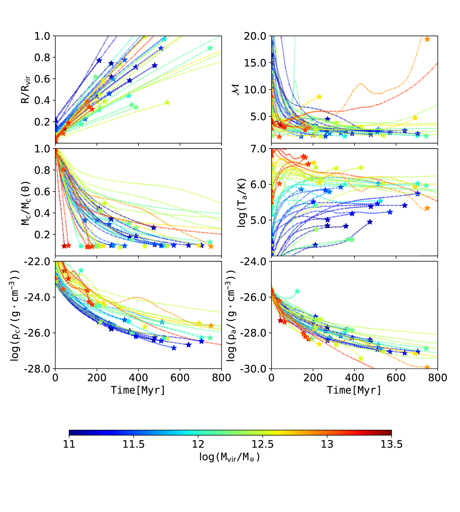
Figure 1 shows how the properties of PhEW particles and their surrounding ambient medium change over time, with the stars showing the disintegration time. We select those particles that are launched shortly after redshift $z=1.0$ from the l50n288-phew-m5 simulation. We choose $z=1$ for this and some of the later analyses because there are relatively large amounts of wind particles in various haloes covering a wide range of halo mass, but the results are similar at other redshifts because wind evolution is only dependent on the local physical properties of the ambient gas and is therefore not directly dependent on the redshift. In general, there are much more winds launched from the low-mass haloes at any given time, but here we choose to show a sample of particles whose host haloes are evenly distributed across $M_{\mathrm{vir}}$ to demonstrate different wind behaviours in haloes of different masses.

The top panels show how far the cloudlets can travel (left panel) in their host haloes and how quickly they slow down relative to the ambient medium. The middle left panel shows how quickly the cloudlets lose their mass. Most cloudlets lose mass gradually over time and survive long enough to travel far from their host galaxies and even beyond their haloes before they disintegrate. The ram pressure and the gravity slow down the cloudlets rapidly at the beginning but become less efficient later on. Most cloudlets remain supersonic with $\mathcal{M}\gtrapprox 1$ until disintegration.

Thermal conduction has little effect except in the most massive haloes, where the hot CGM gas ($T_{\mathrm{a}}>10^{6.5}\,\mathrm{K}$) causes the cloudlets to evaporate within hundreds of Megayears. The linear factor $f_{\mathrm{s}}$ controls the strength of thermal conduction, but changing this parameter slightly does not help the cloudlets survive in the massive haloes, because of the strong non-linear dependence between the conductive flux and the ambient temperature.

The bottom panels show the density of the cloudlets, $\rho_{\mathrm{c}}$ (left panel), and the ambient density, $\rho_{\mathrm{a}}$ (right panel). Both the cloudlet density and the ambient density decrease with time as a PhEW particle travels towards the outer regions of its host galaxy. The ambient density decreases as the radius increases and at the same time the cloudlets expand in the radial direction to adjust to the change in ambient pressure. Even so, at later times the cloudlets are still much denser than the ambient medium because, firstly, the cloudlets are much cooler than the surrounding CGM gas, especially in the hot haloes, and secondly, the cloudlets are mostly still travelling at supersonic speeds and experience a large confining ram pressure.

Figure 2: How far PhEW particles travel in galactic haloes of different masses. From top to bottom, the panels show the time, physical distances and normalised distances that PhEW particles travel on average at the times when they have 75% ($t_{75}$; purple), 50% ($t_{50}$; red), 25% ($t_{25}$; orange) of their original mass remaining, and at the time when they are removed ($t_{last}$; yellow). The PhEW particles in this figure are launched at $z=1$ in the l50n576-phew-m5 simulation. The shaded regions indicate the 20th to 80th percentiles.

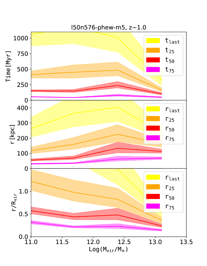
Figure 2 shows statistically how far the PhEW particles travel in haloes of different virial masses. The upper panel and the middle panel show the average time and the average distances that the PhEW particles have travelled, respectively. The different colour lines indicate when and where they have lost 25%, 50%, and 75% of their mass and when they are removed (the disintegration time), as indicated. In general, the PhEW particles from massive haloes travel a further distance owing to their higher initial velocities. However, the PhEW particles can travel hundreds of kiloparsecs regardless of their host haloes.

The lower panel of Figure 2 shows the distances normalised to the virial radius, i.e., $r/R_{\mathrm{vir}}$. In low-mass and intermediate-mass haloes with $\log(M_{\mathrm{vir}}/M_{\odot})<12.5$, the normalised distances are largely independent of the halo mass. On average, the PhEW particles are capable of getting close to the virial radius before they disintegrate, though they have lost half of their mass when they reach approximately 0.25 $R_{\mathrm{vir}}$, depositing half of the wind material within this radius. In massive haloes, conductive evaporation quickly starts to dominate the mass loss and leads to a rapid disintegration of the cloudlets. The time and radius at which the cloudlet disintegrates strongly correlates with the halo virial mass in these massive haloes as a consequence of the strong dependence between the evaporation rate and the gas temperature.

To understand the scalings between the PhEW particle mass loss rate and the halo virial mass, note that in low-mass haloes, hydrodynamic instabilities such as the Kelvin-Helmholtz instability (KHI) dominate the mass loss from the cloudlets as the halo gas is primarily cold (Kereš et al., 2005, 2009). In haloes above about $10^{11.7}M_{\odot}$ a halo of hot gas develops from accretion shocks and hence conductive evaporation becomes increasingly important. In the KHI dominated haloes, both the wind velocities and the sound speed of the ambient medium scale as $M_{\mathrm{vir}}^{1/3}$, approximately. Compression from ram pressure determines the cloudlet density so that $\rho_{\mathrm{c}}\propto v_{\mathrm{rel}}^{2}$, while the cloudlet radius scales with the cloudlet density as $R_{\mathrm{c}}\propto\rho_{\mathrm{c}}^{-1/3}$. Therefore, Equation 17 suggests that $\dot{M}_{\mathrm{c,KH}}\sim M_{\mathrm{vir}}^{2/9}\rho_{\mathrm{a}}^{1/2}$, i.e., the mass loss rate from the KHI depends only weakly on the halo mass at the same ambient density. In practise, the PhEW particles last longest in the intermediate-mass haloes. This is because when the ambient temperature becomes hot ($T_{\mathrm{vir}}>10^{6}\,\mathrm{K}$) in these relatively massive haloes, thermal conduction becomes strong enough to suppress the KHI but is not strong enough to cause significant conductive evaporation.

In Brüggen & Scannapieco (2016) as well as many other cloud-crushing simulations, the cloud often disintegrates over short time-scales, e.g., a few cloud-crushing times. The inability of cold clouds to survive is often used as an argument for why outflows cannot explain cold absorption at large distances in massive halos (e.g. Zhang et al., 2017). In our PhEW simulations, however, the wind particles often survive much longer. The survivability of the clouds in PhEW is controlled by the parameter $f_{\mathrm{KH}}$ for low-mass haloes and the parameter $f_{\mathrm{s}}$ in massive haloes. Both parameters depend on various factors that are not accounted for in idealized simulations such as in Brüggen & Scannapieco (2016). For example, clustered star formation might clear out low density regions in the path of the winds making them easier to escape. Tangled magnetic fields suppress both KHI and conduction by an uncertain fraction. Moreover, the short lifetimes of clouds in the cloud-crushing simulations partly owe to the sometimes large uniform ambient densities, while in cosmological simulations, the ambient density usually decreases as the wind particles move out in the halo.

Figure 3: The median and the 20th to 80th percentiles of the physical distances that the PhEW particles travel at the time when they only have 25% of their original mass. We compare five simulations to show the effects of changing the numerical resolution and the initial cloudlet mass $M_{\mathrm{c}}$. The mass evolution of cloudlets is resolution independent. The smaller mass cloudlets lose mass more rapidly in haloes where thermal conduction is important.

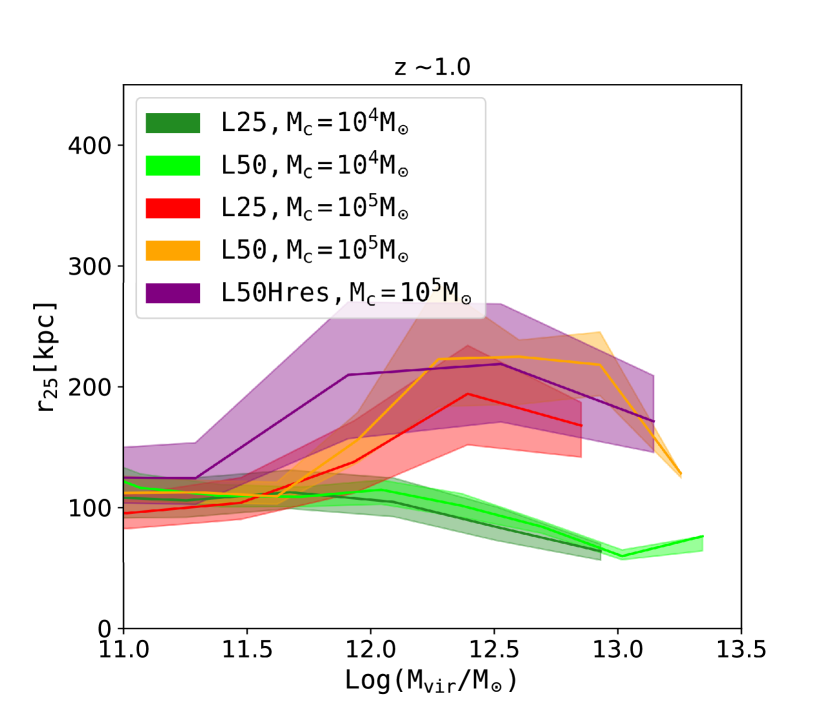
Figure 3 compares the physical distances at which the cloudlets retain only 25% of their original mass between simulations to demonstrate how the wind parameters and numerical resolution affect the distances that the PhEW particles travel. When we assume more massive cloudlets, i.e., $M_{\mathrm{c}}=10^{5}M_{\odot}$, they travel about the same distances in haloes with $\log(M_{\mathrm{vir}}/M_{\odot})<12$, but survive significantly longer in more massive haloes than the PhEW particles that have $M_{\mathrm{c}}=10^{4}M_{\odot}$. In the less massive haloes where the KHI dominates the mass loss, we compensate for the smaller mass of the cloudlets in the $M_{\mathrm{c}}=10^{4}M_{\odot}$ simulations by using a $f_{\mathrm{KH}}$ factor that is approximately 3 times larger. In the more massive haloes, thermal evaporation becomes increasingly important but the total evaporation time is longer for the more massive cloudlets, which scale as $M_{\mathrm{c}}^{-2/3}$(Huang et al., 2020b).

Importantly, Figure 3 also demonstrates that increasing the mass resolution by a factor of eight, i.e., going from the l50n288-phew-m5 simulation to the l50n576-phew-m5 simulation, or changing the box size by a factor of two, i.e., going from the l25n288-phew-m5 simulations to the l50n576-phew-m5 simulations, does not change $v_{\mathrm{25}}$ significantly in haloes of any mass, the change being at most 50%. This resolution insensitivity of the PhEW model is likely better than other sub-grid wind algorithm that under-resolve wind - halo interactions, as a future convergence test of, e.g., $v_{\mathrm{25}}$, could demonstrate. For example, Davé et al. (2016) find that much of the lack of resolution convergence likely occurs because of poor convergence in wind recycling, owing to wind-ambient interactions being highly resolution dependent.

Since the mass and metals that a PhEW particle loses are mixed into the ambient medium, Figure 3 also suggests how wind material is distributed within the haloes. In simulations without the PhEW model, the metal rich wind material is locked to the wind particles. The material does not mix with the halo gas and could only fuel future star formation through wind recycling (Oppenheimer et al., 2010; Anglés-Alcázar et al., 2017). With the PhEW model, the halo gas is constantly enriched by the PhEW particles that pass through. We, therefore, expect that the structures of cold gas, cooling and accretion within the gaseous haloes will be very different between simulations with and without PhEW, as we will show in Section 5.2 and Section 5.4.

Figure 4: Upper panels: The relation between the wind velocities at 0.25 $R_{\mathrm{vir}}$, i.e., $v_{\mathrm{25}}$, and the halo circular velocities $v_{\mathrm{cir}}$. In each panel, the cyan line indicates the medians of $v_{\mathrm{25}}$ and the colour scales indicate the scatter from the relation. The red ($v_{init}$) lines indicate the wind velocity at launch. The black solid and black dashed lines are the 50th and the 95th percentiles from (Muratov et al., 2015), respectively. Lower panels: The grey histograms show the distribution of $v_{\mathrm{cir}}$ for all selected wind particles. The black lines show the fraction of wind particles in each $v_{\mathrm{cir}}$ bin that were able to reach 0.25 $R_{\mathrm{vir}}$ in their host haloes. From left to right, the first row shows results for the gizmo simulation without the PhEW model, and the second and third rows show results both with the PhEW model but at lower and higher resolutions, respectively, as labelled.

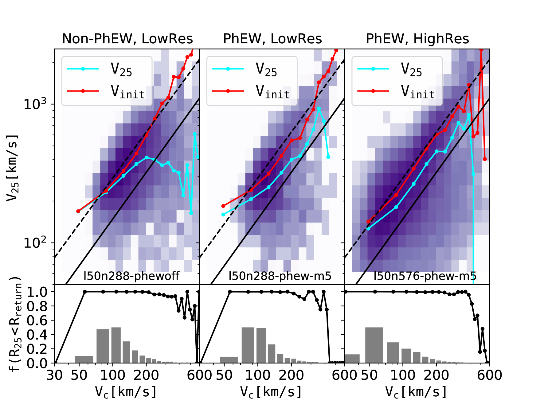
Figure 4 shows the scalings between the wind velocities and the circular velocities, $v_{\mathrm{cir}}$, of their host haloes. In each panel, the colour scale indicates the velocities at 0.25 $R_{\mathrm{vir}}$ and the blue lines show the medians for each halo mass bin. We compare this scaling relation from our simulations to the results from high resolution zoom-in simulations (Muratov et al., 2015). The solid and dashed lines in this figure indicate their 50th and 95th percentiles wind velocities, respectively. The bottom panels show the fraction of wind particles in each halo mass bin that are fast enough to reach 0.25 $R_{\mathrm{vir}}$.

The wind speed scalings in our simulations align better with the 95th percentile from Muratov et al. (2015) than their median because of the different ways of measuring the wind speed (Huang et al., 2020a). In Muratov et al. (2015), the wind speed is averaged over all outflowing particles at 0.25 $R_{\mathrm{vir}}$, effectively measuring the bulk motion of all the halo gas at that radius. In our simulations, we average over wind particles only, which should correspond to the fastest outflowing particles in a halo. Therefore, it is more reasonable to compare the wind speed measured in our simulations to the 95th percetile from Muratov et al. (2015).

In Huang et al. (2020a), we adjusted the wind launch velocities in our SPH simulations using gadget-3 to recover the superlinear scaling relation from Muratov et al. (2015) (see the appendix). Most of the winds in the SPH simulations were then fast enough to reach 0.25 $R_{\mathrm{vir}}$ regardless of the halo mass. However, in the gizmo simulation without the PhEW, even though we use the same wind launch velocities, the winds slow down more quickly in massive haloes and many of them stop and turn back before reaching 0.25 $R_{\mathrm{vir}}$ (left panel of Figure 4).

In the gizmo simulations with the PhEW model, however, the scaling relation is not only consistent with Muratov et al. (2015) but also much less dependent on the numerical resolution. In both the SPH and the gizmo simulations without the PhEW, increasing the numerical resolution tends to slow down winds even more quickly. In practise, we need to boost the initial wind velocities by a factor of 1.14 in the SPH simulations when increasing the spatial resolution by a factor of two (a factor of eight increase in mass resolution) to obtain the same $v_{\mathrm{25}}-v_{\mathrm{cir}}$ scaling relation (Huang et al., 2020a). In PhEW simulations, one no longer needs to re-tune the wind velocities to match the Muratov et al. (2015) relations at different resolutions as in the non-PhEW simulations.

Hence, the PhEW model has the advantage that the dynamics of the wind particles are governed by analytic equations, and thus will be less affected by unresolved or poorly resolved wind-CGM hydrodynamic interactions.

In the PhEW simulations, fewer wind particles reach 0.25 $R_{\mathrm{vir}}$ in massive halos as they have lost most of their mass before they reach that radius in these halos. Typically the fraction of wind particles that reach 0.25 $R_{\mathrm{vir}}$ starts dropping significantly above $v_{\mathrm{cir}}\approx 300$ km s^-1, corresponding to haloes with virial temperatures over 10 million degrees. Clouds in these haloes evaporate on very short time- scales.

Figure 5: The density–temperature gas phase diagram at $z=0.25$ with PhEW particles over plotted. The background scale indicates the mass distribution in this phase space. The two dotted lines separate the phase space into warm-hot gas, hot gas, diffuse intergalactic gas, and condensed gas phases. For each PhEW particle, we show its cloudlet properties, i.e., $\rho_{\mathrm{c}}$ and $T_{\mathrm{c}}$, as a cross and its ambient properties, i.e., $\rho_{\mathrm{a}}$ and $T_{\mathrm{a}}$ as a circle. The size and colour of the symbol indicates the remaining cloudlet mass fraction and the time since it became a PhEW particle, i.e., $t_{\mathrm{out}}$, respectively. The cloudlets (crosses) are clustered at $T_{\mathrm{c}}\approx 10^{4}\,\mathrm{K}$. Older winds tend to have a smaller cloudlet mass and have travelled further into the lower density regions. In particular, there are PhEW particles that have survived for more than 5 gigayears. Most of them are in the most diffuse regions of the Universe.

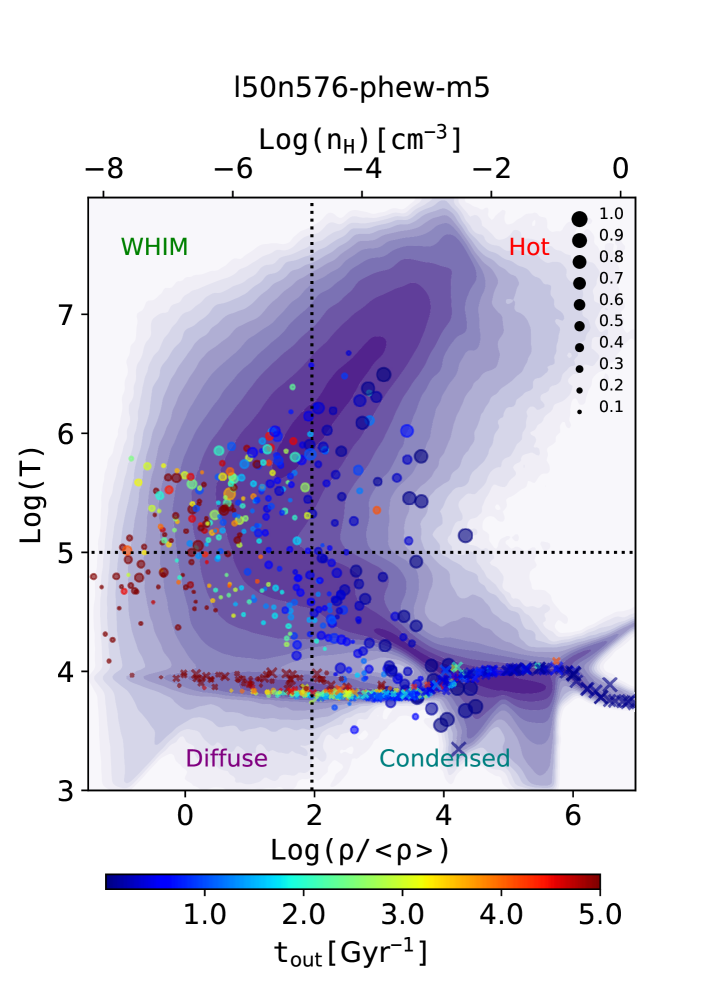
Figure 5 shows how the baryonic mass distributes according to its density and temperature. We only show the result from the fiducial l50n576-phew-m5 simulation here, but the phase space distributions are similar between different simulations in this paper.

At $z=0.5,$ PhEW particles have a wide range of properties, such as $M_{\mathrm{c}}$, $\rho_{\mathrm{c}}$ and the age, $t_{\mathrm{out}}$, i.e., the age of the winds since they were launched. The PhEW particles exist in various halo environments with different ambient properties. A typical PhEW particle in this diagram travels from the cold, dense interstellar medium (ISM) and moves across the phase diagram towards lower densities, with its cloudlet masses decreasing with time. However, most PhEW particles are at an equilibrium temperature of around $T_{\mathrm{c}}\approx 10^{4}\,\mathrm{K}$ over their lifetimes regardless of the ambient temperature of the surrounding gas, as a result of strong metal line cooling inside the cloudlet. This picture is consistent with high-resolution cloud-crushing simulations. The cloudlet densities, on the other hand, decrease with time as the cloudlets expand as they enter more diffuse regions. The cloudlet density is often a few orders of magnitude larger than the ambient density owing to compression from ram pressure and the contrast between the cloudlet temperature and the ambient temperature.

The PhEW particles often travel at high speed and decelerate slowly owing to their small cross-sections, so they leave the central regions of their host haloes very soon after launch and are, therefore, more likely to be found in the diffuse and the WHIM gas at any given time.

Some PhEW particles survive for a very long time and can be found in very diffuse regions of the simulation. Cloudlets in these PhEW particles will have expanded greatly and become kpc-scale metal rich structures in the IGM. Most of these long lived wind particles were launched from galactic haloes with $12.0<\log(M_{\mathrm{vir}}/M_{\odot})<13.0$, corresponding to a temperature range where mass loss is minimal because there is still enough conduction to suppress the Kelvin-Helmholtz instabilities but not enough to promote rapid conductive evaporation. However, they only represent a small fraction of the total amount of winds launched from these haloes over time. For example, of all the winds launched from these haloes at $z=1$, less than 10% have ages over 5 gigayears, and the fraction is much less in other haloes.

4.2 Wind Recoupling

In our fiducial model, we eliminate PhEW particles from a simulation when the cloudlet mass drops below a certain fraction $f_{\mathrm{lim}}$. In most circumstances, if a gas particle has been launched as a wind, it will either remain as a PhEW particle or disintegrate. In this section, we consider recoupling the PhEW particles that become sub- sonic, i.e., turning them back into normal gas particles when they still have more than $f_{\mathrm{lim}}$ of their original mass, and we explain why we decided not to let them recouple in our final PhEW model.

In a test simulation, l50n288-phew-m5-rec, we allow PhEW particles to recouple when they have slowed down to a sub-sonic speed relative to the surrounding medium, i.e., $\mathcal{M}<\mathcal{M}_{\mathrm{re}}$, where $\mathcal{M}_{\mathrm{re}}$ is a parameter that we set to 1.0 in our test simulation. When a PhEW particle recouples, it becomes a normal gas particle that starts interacting with its neighbouring particles hydrodynamically while retaining its current mass and velocity.

Figure 6: The evolution of cloud mass ($M_{c}/M_{c}(0)$) as a function of Mach number ($\mathcal{M}$) for the PhEW particles launched at $z=1$ in the l50n288-phew-m5-rec simulation. The star symbols indicate the last appearance of these PhEW particles in the simulation. In all the PhEW simulations, we remove PhEW particles when their mass drops below 10%, indicated as the horizontal dotted line. In the l50n288-phew-m5-rec simulation shown here we also allow PhEW particles to recouple at $\mathcal{M}<1.0$, which is indicated as the vertical dotted line. There is also a small fraction of PhEW particles that have neither recoupled nor disintegrated at the end of the simulation. In practise, most particles have lost enough mass before slowing down to meet the recoupling criterion.

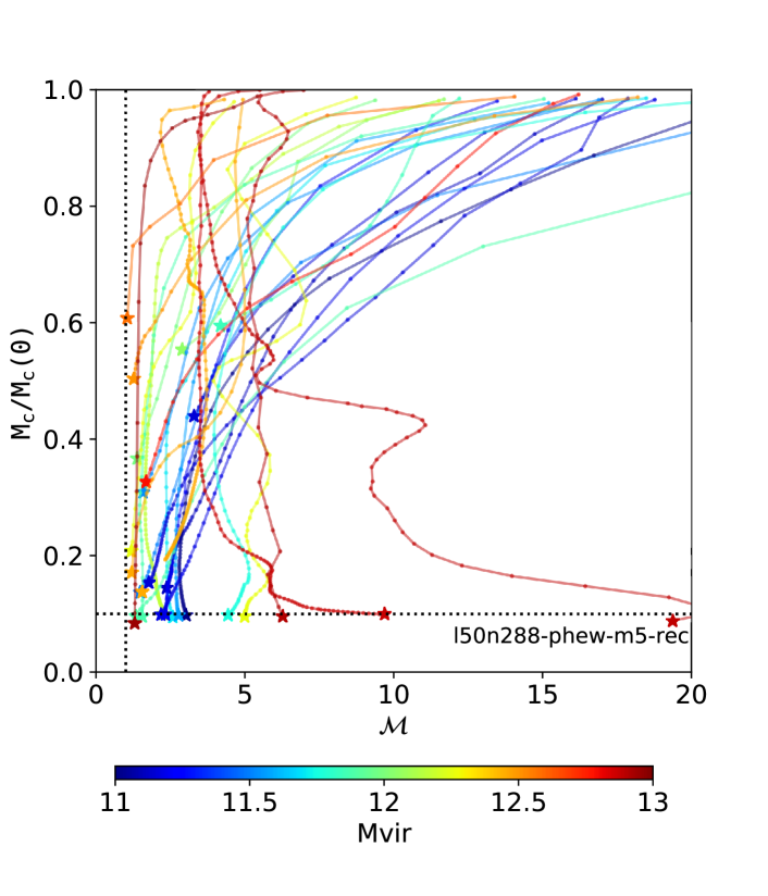
Figure 6 tracks the evolution of the PhEW particles before they either recouple or disintegrate in cloud mass–mach number space. Asymptotically, most PhEW particles end up in a narrow region of this space where both the cloudlet mass and the mach number are small. Winds from low-mass haloes ($\log(M_{\mathrm{vir}}/M_{\odot})<12.5$) often start with a high mach number but gradually slow down and still retain a considerable amount of cloudlet mass at the time of recoupling. On the other hand, winds from massive haloes evaporate much more quickly while staying at a nearly constant speed. Figure 6 also shows a few particles from massive galaxies with increasing $\mathcal{M}$ at later times as a result of their surrounding medium becoming cooler as they travel outwards.

Our test simulations also show that there are a small fraction of PhEW particles that neither recouple nor disappear. Nearly all of them are launched from intermediate-mass haloes ($\log(M_{\mathrm{vir}}/M_{\odot})\approx 12.0$) and have travelled beyond the virial radius of their host haloes, where both the mass loss rate and the deceleration rate are very small, enabling them to stay as PhEW particles for a long time. In our simulations, we find that around 10% to 15% of wind particles launched from these haloes show this behaviour.

In our fiducial model, we remove a PhEW particle once its mass drops below $f_{\mathrm{lim}}=0.1$, indicated as the horizontal dotted line. Alternatively, one might think of letting it recouple as a normal gas particle once its mach number becomes low enough, but, we found that the recoupled particles will often numerically overheat even if one uses a low mach number for the recoupling criteria (e.g. $\mathcal{M}_{\mathrm{re}}=1$ as the vertical dotted line in the figure). We experimented by making even stricter recoupling criteria. This led to wind particles remaining as PhEW particles for longer periods of time before recoupling, during which time they typically retained a low temperature. But, whatever the recoupling criteria, once the PhEW particles became ordinary gas particles again, they quickly heated from about $10^{4}$ K up to $10^{5}\sim 10^{7}$ K.

This over-heating occurs because recoupling a cold PhEW particle to a hot ambient medium leads to a sudden change in the estimated density of that particle. At the time of recoupling, the density of the particle changes from the cloud density to the ambient density. Before recoupling, one uses the density of the clouds to compute the cooling rate, while after recoupling, one uses the kernel smoothed ambient density, which is lower than the cloudlet density by a factor of $\chi\approx T_{\mathrm{a}}/T_{\mathrm{c}}$. This often leads to an order of magnitude decrease in the density estimation. As a result, the cooling rate drops immediately at the time of recoupling, enabling the particle to heat up very quickly.

Therefore, we do not allow PhEW particles to recouple in our simulations owing to this numerical artefact. Our test simulations show that whether or not we allow recoupling has little effect on galaxy properties because a particle usually has lost most of its mass before meeting the recoupling criteria and this choice, therefore, plays a limited role in determining galaxy properties. However, this experiment should serve as a warning to any cosmological simulation that attempts to include the effects of galactic supernova winds or AGN winds by adding velocities to individual particles. Such methods might lead to a spurious heating of those particles compared to a simulation that had orders of magnitude more resolution, since the evolution of the particle temperature may be sensitive to numerics.

Finally, a PhEW particle may travel into a galaxy, whose further evolution is beyond the scope of the PhEW model. Therefore, we let any PhEW particle whose ambient density is larger than $\rho_{\mathrm{SF}}$ become a normal gas particle. However, this affects very few PhEW particles (typically $\ll 0.1\%$).

5 Galaxy and Halo Properties

5.1 The Stellar Masses of Galaxies

Figure 7: Galactic stellar mass functions at $z=0$, $z=1$, $z=2$ and $z=4$. We compare the results from different simulations that are coloured in accordance with inset key. The two dashed lines correspond to the two non-PhEW simulations. The bold lines correspond to the simulations with a higher resolution. See Table 1 for details. The vertical dotted and dashed lines indicate the mass resolution limit corresponding to a total mass of 128 gas particles in the low-resolution and high-resolution simulations, respectively.

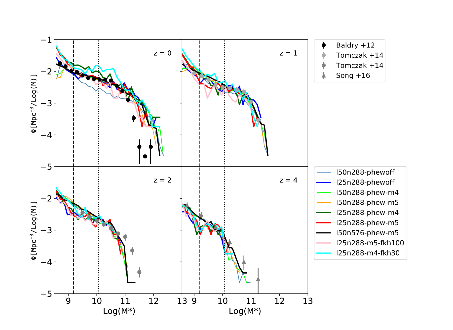
Figure 7 shows the galactic stellar mass functions (GSMFs) at different redshifts. In the simulations without the PhEW, we adjust wind parameters that control the mass loading factor and the initial wind velocities so that the GSMFs match observations (Huang et al., 2020a). In the simulations with the PhEW, we use the same set of wind parameters but also adjust the $f_{\mathrm{KH}}$ parameter for each choice of $M_{\mathrm{c}}$. Since a smaller cloudlet loses mass more quickly, we adopt a larger value of $f_{\mathrm{KH}}$ in the simulations with $M_{\mathrm{c}}=10^{4}M_{\odot}$.

The GSMFs from the different PhEW simulations with volume sizes and mass resolutions that vary by a factor of eight are nearly indistinguishable as long as they use the same PhEW parameters such as $f_{\mathrm{KH}}$, but the low resolution simulation without the PhEW, i.e., l50n288-phewoff, under-produces stars at $z=0$ relative to other simulations. The results from the PhEW simulations are much more resolution independent, regardless of the choice of the cloudlet size. Surprisingly, in the simulations including the PhEW model, the galactic stellar mass functions remain viable below the nominal resolution limit that we established previously of 128 gas particle masses (Finlator et al., 2006), down to a mass of 16 gas particle masses as one can see by comparing the lower resolution l50n288-phew-m5 simulation with the higher resolution l50n576-phew-m5 simulation.

On the other hand, changing the PhEW parameters may lead to significant differences in the results. For example, increasing the $f_{\mathrm{KH}}$ parameter help clouds resist hydrodynamic instabilities and enhances their lifetime in low-mass haloes. As a result, the winds from the l25n288-m5-fkh100 simulation generally survive longer than in the l25n288-phew-m5 simulation, resulting in less star formation at $z<1$. On the contrary, the winds from the l25n288-m4-fkh30 simulation disintegrate faster than in the l25n288-phew-m4 simulation, leading to more recycling and star formation.

Figure 8: Stellar mass - halo mass relations at $z=0$ from the same set of simulations in Figure 7. We show the observational results from Behroozi et al. (2013) (data points with error bars) and Moster et al. (2018) (purple solid line) for comparison. The vertical dotted line indicate the mass resolution limit corresponding to a total mass of 128 dark matter particles in the low-resolution simulations. The mass resolution limit of the high-resolution simulations is below the plotting limit of this figure.

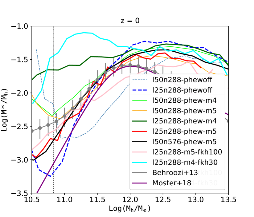
Figure 8 shows a similar result. The $z=0$ stellar mass–halo mass (SMHM) relations between the two simulations without PhEW are significantly different at almost every $M_{\mathrm{h}}$, while the simulations with PhEW are much more consistent with each other. In particular, the galaxies in low-mass haloes are more massive in the PhEW simulations, in better agreement with observational results from (Behroozi et al., 2013) but worse compared to Moster et al. (2018).

Figure 9: The composition of baryons in galactic haloes at $z=0$ (left panel) and $z=2$ (right panel). Each panel shows the mass of the different components, cold gas (blue), hot gas (red), star-forming gas (orange) and the total baryons (gas + star, grey), as fractions of the cosmic mean value with halo mass. The solid lines and the shaded regions indicate the medians and the 68 percentiles from the l50n576-phew-m5 simulation. The dashed and the dotted lines are from the l50n288-phew-m5 and the l50n288-phewoff simulations, respectively. On the top axis of the panels, we label the average stellar masses of the central galaxies in corresponding haloes from the l50n576-phew-m5 simulation.

5.2 Baryonic Mass Distributions

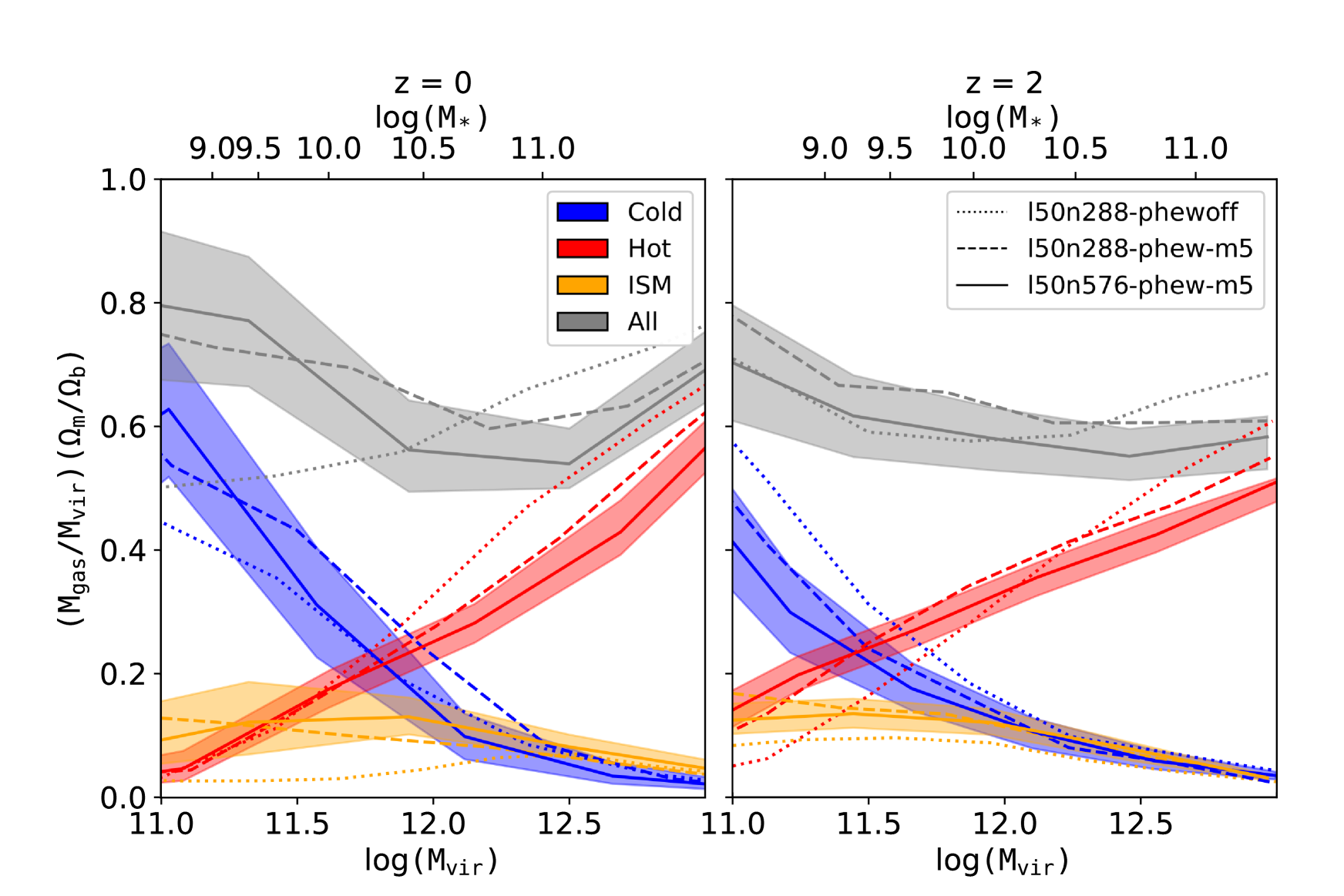
Figure 9 compares the amount of baryons in different phases normalised by the cosmic mean baryon fraction. For each central halo, we separate cold and hot gas with a temperature threshold of $T_{\mathrm{cut}}=10^{5.0}\,\mathrm{K}$, close to the range of temperatures where the fractions of many observed ions are very sensitive. In previous papers, we used a slightly higher threshold of $10^{5.5}\,\mathrm{K}$ (Kereš et al., 2005; Huang et al., 2020a), but the difference between these values has little effect on the cold gas fraction. In addition to cold and hot halo gas, we also show the mass of star-forming gas in the galaxies and the total baryonic mass including stars.

The fraction of hot gas in galactic haloes depends strongly on the halo mass but is less sensitive to the different numerical models. The halo gas switches from mostly cold to mostly hot at around $\log(M_{\mathrm{vir}}/M_{\odot})=12.0$. This threshold is somewhat higher than in Kereš et al. (2005), owing to the inclusion of metal line cooling (Gabor & Davé, 2012). In general, the different wind models do not significantly affect the amount of hot gas in galactic haloes of any given mass. This is also true when we change the PhEW parameters and the numerical resolution.

The baryon fraction within haloes is less than 75% of the cosmic mean baryon fraction in most haloes, regardless of which code or which wind model we use. This depletion of halo baryons is the result of winds that escape from haloes over time. The PhEW simulations have a similar fraction of wind material escaping from haloes as the non-PhEW simulations. The escape fractions are also similar at $z=0$ and $z=2$, indicating that most of the winds escape at higher redshifts.

Figure 10: The average radial profiles in galactic haloes selected by halo mass at $z=0.25$. The left panels show total baryon mass profiles including winds. In each radial bin, we separate the baryons into cold gas (blue), hot gas (red) and star-forming gas (brown) as described in the text. The right panels show the total fraction of wind material (orange) as a function of radius. We also separate the wind material into cold wind (cyan), hot wind (magenta) and PhEW particles (green, only existing for the PhEW simulations). From top to bottom shows averaged profiles for low- mass, intermediate-mass and massive haloes, with their corresponding mass ranges indicated in the right panels. The dashed and solid lines compare results from the l50n288-phewoff and the l50n288-phew-m5 simulations, respectively.

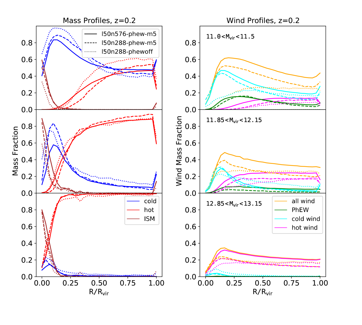
Figure 10 shows how wind particles affect the radial distribution of baryons and wind material in galactic haloes with different $M_{\mathrm{vir}}$. In the left panels, we calculate the mass fraction of the cold, hot and star-forming gas and wind particles as a function of the normalised radius $r/R_{\mathrm{vir}}$ for each halo and average over all central haloes within the same $M_{\mathrm{vir}}$ range. We define star forming gas as dense gas particles residing in galaxies that satisfy the star-forming criteria that we use during the simulations, and we separate cold halo gas from hot halo gas based on the temperature criterion $T<10^{5.0}\,\mathrm{K}$. Consistent with Figure 9, the fraction of cold and hot gas as a function of halo radius is similar between non-PhEW and PhEW simulations, especially in the intermediate and massive haloes.

In the right panels of Figure 10, we show the fraction of wind material in each radial bin. For the non-PhEW simulation, we define wind material as gas particles that were once launched as winds, and we further separate them into cold winds or hot winds based on their current gas temperature. These particles often have distinct properties from their neighbouring normal gas particles, e.g., a higher metallicity as they were enriched in the galaxies before becoming winds. In the PhEW simulations, wind particles mostly disintegrate after losing most of their mass to the neighbouring particles, so that the wind material is well mixed with the halo gas. For each gas particle, a fraction of its mass has come from a PhEW particle. Therefore, we define the wind fraction in a gas particle as the fraction of the material that used to be in a PhEW particle. In addition, the currently surviving PhEW particles make up a small fraction of the total baryonic mass in the low-mass haloes in the PhEW simulation. This PhEW fraction becomes negligible in more massive haloes because PhEW particles launch less frequently and travel faster through these haloes.

Even though the definition of wind material differs between the non-PhEW and the PhEW simulations, its radial distribution between these simulations is very similar in the intermediate and massive haloes, with a total wind fraction of approximately 30% and 20% at most radii, respectively. However, in the low-mass haloes, the wind fraction in the PhEW simulations is considerably higher. The wind fraction in the PhEW simulation also increases towards smaller radii until the innermost region where star-forming gas dominates, while the wind fraction in the non-PhEW simulation declines within 0.5 $R_{\mathrm{vir}}$ because typical wind particles travel quickly and hence spend little time near the galaxy.

The fraction of hot wind material is also very similar between the two simulations, but the origin of the hot wind differs. In the non-PhEW simulation, the hot wind material is simply high velocity wind particles that heat up to the ambient temperature. In the PhEW simulation, on the other hand, it mostly made up of cloudlets that evaporate and mix into the hot ambient medium.

Although not shown here, the profiles from the l50n288-phew-m4 simulation are nearly identical to the l50n288-phew-m5 simulation, except that it has a slightly higher fraction of PhEW particles in the low-mass haloes.

5.3 Gas Metallicities

Figure 11: Similar to Figure 10, this figure shows how metals are distributed in the different gas phases. The left panels show the fraction of metals in cold gas (blue), hot gas (red) and the PhEW particles (only applying to the PhEW simulation) as a function of radius. Note here we exclude the ISM gas, which dominates at inner radii, from the plot. The right panels shows the metallicity of cold gas (blue), hot gas (hot) and the average of the two in solar units as a function of radius. Here we use $Z_{\odot}=0.0122$ from Asplund et al. (2009).

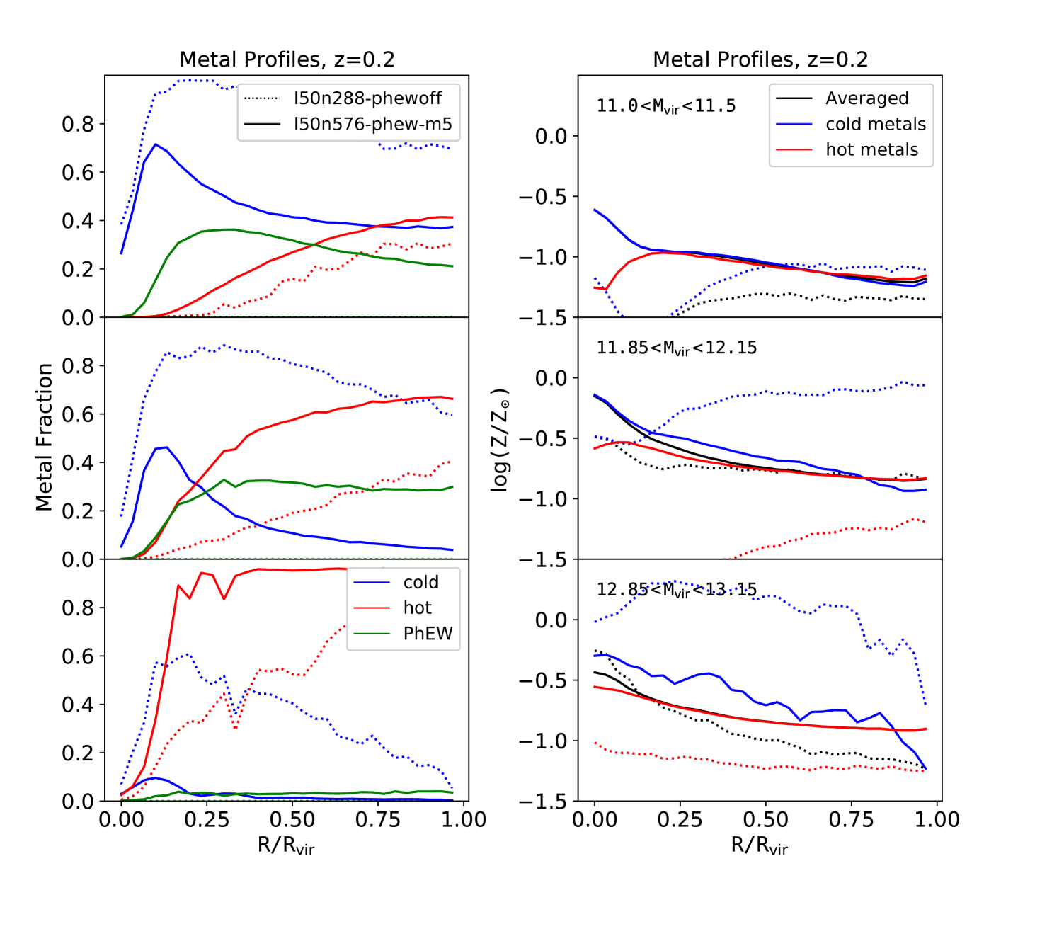
The PhEW particles lose not only mass but also metals to the surrounding medium so the radial distribution of metals also changes significantly with the PhEW model. In the left panels of Figure 11, we study the fraction of metals in each of the gas phases as a function of halo radius. For the non-PhEW simulation, most of the metals are locked in former wind particles and there is no exchange of metals between the former wind particles and normal gas particles. Therefore, one can interpret the cold and hot fraction in the non-PhEW simulation as the fraction of former wind particles that are currently cold or hot.

In the PhEW simulation, $20\%$ to $40\%$ of the metals are in the PhEW particles at most radii in low-mass and intermediate-mass haloes as they survive longer in haloes of these masses. In addition, the fraction of metals in the hot gas tends to increase with radius and halo mass. In the non-PhEW simulation, the majority of metals are in the former wind particles that remain mostly cold. Even in the most massive haloes ($\log(M_{\mathrm{vir}}/M_{\odot})\approx 13.0$), a considerable amount of metals are in the cold wind particles that scatter over all radii. The former wind particles could remain mostly cold surrounded by hot halo gas particles in part because of their high metallicities and in part because the interactions of single particles with the ambient background are not accurately modeled. In contrast, almost all metals are hot in the PhEW simulation owing to the absence of cold gas in these massive haloes and the ability to share metals.

In the right panels of Figure 11, we calculate the metallicity as the ratio of the total mass of metals and the total gas mass for each phase separately. Even though the averaged metallicity profiles are similar between the non-PhEW and the PhEW simulations, the metallicities of the cold and hot gas alone are drastically different. In the PhEW simulations, the metallicities of the cold and hot gas are comparable. However, in the non-PhEW simulations the metallicity of the cold gas is significantly higher, since the metal-rich former wind particles are on average colder than the ambient gas particles owing to more efficient metal cooling, resulting in disproportionally more metals in the cold gas.

In the most massive haloes, the metallicity of the hot gas in the PhEW simulation is much closer to the observed universal value of 1/3 $Z_{\odot}$ for hot cluster gas at low redshifts (e.g. De Grandi & Molendi, 2001; Leccardi & Molendi, 2008; Molendi et al., 2016), while the metallicity in the non-PhEW simulation is much lower than this observed value. Although the halos considered here are low-mass groups rather than clusters, a comparison of cluster metallicity profiles can be undertaken in the future.

Figure 12: Mass weighted histograms of metallicities in low-mass (upper panel), intermediate-mass (middle panel) and massive (bottom panel) haloes at $z=0.25$. We compute the histograms using gas particles within the virial radius and exclude particles that are star forming or that are from the innermost radii ($r/R_{\mathrm{vir}}<0.1$). We normalise the histograms by the total mass of the selected particles. We also show the histograms for the cold (blue) and hot (red) gas separately, using a temperature cut of $\log(T/\,\mathrm{K})=5.0$. The dotted, dashed, and solid lines correspond to the l50n288-phewoff, l50n288-phew-m5, and the l50n576-phew-m5 simulations, respectively. A considerable fraction ($>40\%$) of particles in the l50n288-phewoff simulation have metallicities below the plotting limit of the figure.

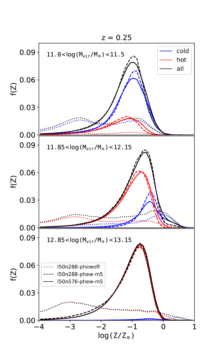
Figure 12 compares the metallicity distributions in the halo gas between the non-PhEW and the PhEW simulations. The two PhEW simulations, l50n288-phew-m5 and l50n576-phew-m5, have very similar distributions regardless of the different numerical resolutions, which is another example of the robustness of the PhEW model. Gas metallicities in the PhEW simulations strongly peak at between $-1<\log(Z/Z_{\odot})<0$ for all of the three halo mass bins. The metallicities in the cold and hot gas have similar shapes except for a slight shift in the peaks. The non-PhEW simulation, on the other hand, has much broader overall metallicity distributions. Over $40\%$ of particles in the non-PhEW simulation even have metallicities below the plotting limit, $\log(Z/Z_{\odot})=-4$, of Figure 12, while the fractions in the two PhEW simulations are negligible. The non-PhEW simulation also shows a clear bimodality in the metallicity distributions in both the low-mass and intermediate-mass haloes. In the intermediate-mass haloes, the metal-rich peak at $\log(Z/Z_{\odot})\approx-0.5$ is dominated by cold gas while the metal-poor peak at $\log(Z/Z_{\odot})\approx-3.0$ is dominated by hot gas.

In the non-PhEW simulations, the bimodal distribution of metals in galactic haloes results from different metallicities in the inflowing and outflowing material (Ford et al., 2014; Hafen et al., 2017) and the inability of these different materials to mix. This inability to mix metals is present in any hydrodynamical simulation where mass exchange between fluid elements is not allowed (e.g. Gizmo-MFM, SPH, and in contrast to e.g. AREPO and all Eulerian grid simulations) and even in simulations that attempt to evolve the winds numerically (e.g. Schaye et al., 2015; Hopkins et al., 2018) since the mixing occurs on scales that cannot be resolved in those simulations.

Many recent simulations (Shen et al., 2010; Brook et al., 2012, 2014; Su et al., 2017; Tremmel et al., 2017; Rennehan, 2021) have implemented sub-grid models to allow metal diffusion following the Smagorinsky (1963) turbulence model. Results from these simulations suggest metal diffusion plays important roles in the chemical evolution of dwarf galaxies (Pilkington et al., 2012; Revaz et al., 2016; Hirai & Saitoh, 2017; Escala et al., 2018). However, the physics underlying these models are very different from those in PhEW model and it is not clear if the impact of the PhEW on distributing metals would be similar to the sub-grid diffusion models adopted in these simulations or not.

In the PhEW simulations, metal mixing can occur naturally between the outflowing wind particles and the ambient medium, which effectively erases the bimodality. Observationally, whether or not a bimodality exists at low redshifts is still uncertain (Lehner et al., 2013; Prochaska et al., 2017). Future quasar absorption line observations could potentially distinguish different models of how metals mix in the CGM. Furthermore, although these results hint at major differences in the predicted metallicity distributions in the different wind models, our cold-hot temperature split is only a crude attempt to make contact with the observations. To make more robust comparisons with the observations of gas metallicities requires simulated quasar absorption lines, which we will pursue in future work.

Despite the fact that the PhEW model drastically changes the distribution of metals in the CGM, it hardly affects the metallicities of the star-forming gas in the simulated galaxies. We find that the mass-metallicity relation in the simulations without PhEW are nearly identical to that in the simulations with PhEW.

5.4 Gas Accretion

The gas that ultimately forms stars in galaxies had different thermal histories before accretion. Galaxies may acquire gas through cold accretion, hot accretion and wind re-accretion and their relative importance strongly depends on the galaxy or dark halo mass (Kereš et al., 2005, 2009; Oppenheimer et al., 2010). In simulations without PhEW, one often defines wind re-accretion as the accretion of former wind particles. The definition is clear since the wind particles do not mix with other particles.

In simulations with the PhEW, the mass of a normal gas particle can grow by a considerable amount owing to material lost from neighbouring PhEW particles before the gas particle accretes onto a galaxy. We define the wind mass, i.e, $M_{\mathrm{w}}$, of a gas particle as the mass that came from PhEW particles. At the time when a gas particle accretes, we count its wind mass as wind re-accretion and the rest of its mass as pristine accretion. In non-PhEW simulations, since there is no mass exchange between normal gas particles and wind particles, we define pristine accretion as the accretion of a gas particle that has never accreted onto any galaxy before, and wind re-accretion as the accretion of particles that used to be winds. This definition for the non-PhEW simulations is identical to our previous papers (Oppenheimer & Davé, 2008; Huang et al., 2020a).

For each PhEW particle we note the time it was launched, $t_{w}$, and the velocity dispersion, $\sigma_{w}$, of the galaxy that launches it in a wind. Therefore, whenever a gas particle acquires some mass from a PhEW particle, we can calculate the mass-weighted average wind launch time, $\bar{t}_{w}$, and the mass-weighted velocity dispersion of the wind launching galaxy $\bar{\sigma}_{w}$ for the wind component of the gas particle. We find that the variances for $t_{w}$ are usually large while the variances for $\sigma_{\mathrm{gal}}$ are usually small, indicating that a gas particle typically accumulates its wind material over a long period of time but mostly from winds launched from the same halo.

Figure 13: The relative importance of different accretion types for galaxies of different mass. In the upper panel, we calculate for galaxies at $z=0$ how much of their total stellar masses (black) came from cold accretion (blue), hot accretion (red) or wind re-accretion (green). The lower panel shows their relative fractions. In each panel, the dotted lines are from the l50n288-phewoff simulation, which defines cold accretion, hot accretion and wind re-accretion similar to Oppenheimer et al. (2010). The solid lines are from the l50n576-phew-m5 simulation, using the definitions described in the text. The results from the l50n288-phew-m5 simulation are similar to the l50n576-phew-m5, so we do not plot them on this figure for a cleaner visualization.

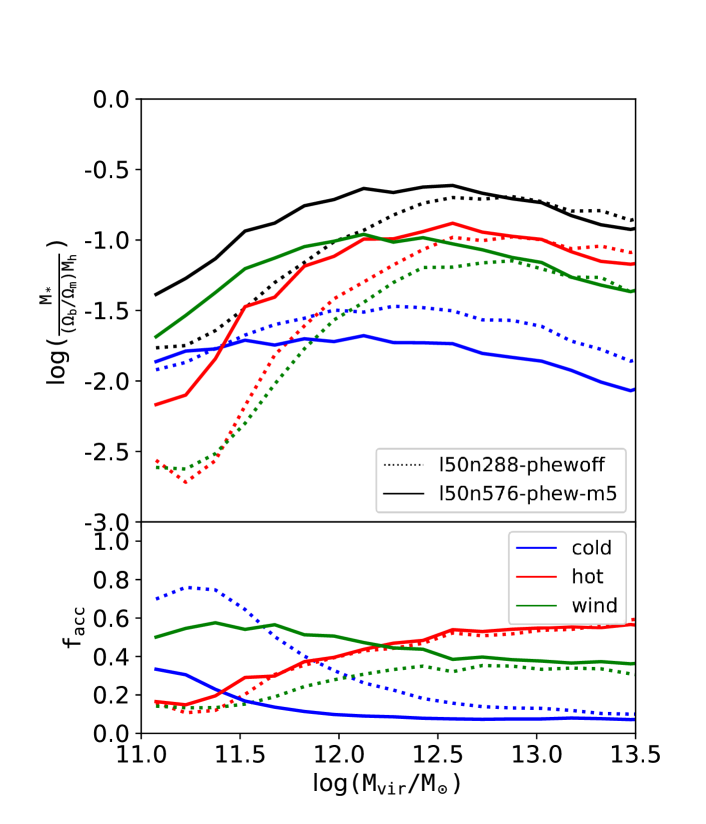
In Figure 13, we look at the thermal histories of gas particles before they accreted onto galaxies and formed stars. For each galaxy at $z=0$, we consider all star particles of each galaxy, and for those that accreted onto the galaxy as gas, determine whether they were cold accretion, hot accretion or wind re-accretion. The accretion event associated with a star particle is the last time that a gas particle accretes onto a galaxy before becoming a star particle, when its density rises above the star formation density threshold $\rho_{\mathrm{SF}}$. In a non-PhEW simulation, each accretion event can only be one of the three types, while in a PhEW simulation, each accretion event can be a mix of wind re-accretion and either of the two other types. In this analysis, we separate cold accretion from hot accretion using a temperature cut of $T_{\mathrm{max}}=10^{5.5}\,\mathrm{K}$, where $T_{\mathrm{max}}$ is the maximum temperature that the gas particle reached before accretion.

In the non-PhEW simulation, l50n288-phewoff, cold accretion dominates galaxies in small haloes with $\log(M_{\mathrm{vir}}/M_{\odot})<12.0$ while hot accretion dominates in massive haloes. Hot accretion might become less important if one were to include AGN feedback to efficiently suppress cooling flows in the most massive haloes. The fraction of wind-re-accretion is negligible in very low-mass haloes and grows with halo mass. The importance of wind re-accretion is sensitive to wind model implementations (Huang et al., 2020a). For example, the initial wind speed determines whether or not wind particles can escape haloes of different masses and controls the amount and the time-scale of wind recycling.

Compared to the non-PhEW simulation, the main difference in the PhEW simulation is a significant increase of wind re-accretion in low-mass haloes, making it the dominant mode of accretion in these haloes. Adding this recycled wind material leads to as much as 0.5 dex increase in the low-mass end of the stellar mass - halo mass relation, which now matches the empirical results from Behroozi et al. (2013) as shown in Figure 8. Although not shown here, the results from the low resolution l50n288-phew-m5 simulation are very similar to the l50n576-phew-m5 simulation.

Most winds can easily escape the low-mass haloes in both the PhEW and the non-PhEW simulations. However, a PhEW particle loses its mass as it travels outwards to the cold gas that it passes through and that gas can later accrete unto the galaxy. A star-forming galaxy in a low-mass halo usually has strong winds resulting in a large amount of wind material being mixed with the accreting gas and, therefore, increases the amount of wind re-accretion in a PhEW simulation.

The total amount of cold accretion is similar between the non-PhEW and the PhEW simulations, but the total amount of hot accretion also significantly increases in the PhEW simulations, possibly because the hot gas is more metal rich owing to the mixing with outflowing wind material.

The two PhEW simulations with different resolutions are much more similar. The l50n576-phew-m5 simulations have slightly more hot accretion and wind re-accretion but less cold accretion, but the total amounts of gas accretion in these two simulations are comparable, again demonstrating the robustness of the PhEW model to numerical resolution.

Figure 14: In the upper panel, we show from which haloes (binned by their velocity dispersions) the winds are launched at z = 2 (blue) and at z = 0 (red). The l50n576-phew-m5 simulation (solid lines) launches much more wind in low-mass haloes, which are unresolved in the l50n288-phew-m5 simulation (dashed lines), at both redshifts. In the lower panel, we show the mean $\sigma_{\mathrm{gal}}$ of all wind material that accreted unto the galaxies that are resolved in both simulations within the last gigayear in these simulations.

Why do galaxies in the high resolution simulations accrete more wind material? The reason is that at higher resolution, one can resolve haloes with lower mass in the simulation or haloes at earlier stages of their assembly when they were still too small to be resolved in the lower resolution simulations. These low mass haloes launch a considerable amount of wind material because of their very high mass loading factors before they grow to sizes that would be resolvable in the lower resolution simulations. In their subsequent evolution, galaxies in the high resolution simulations start accreting material from this earlier generation of winds while the galaxies in the low resolution simulation are still accreting mostly pristine gas.

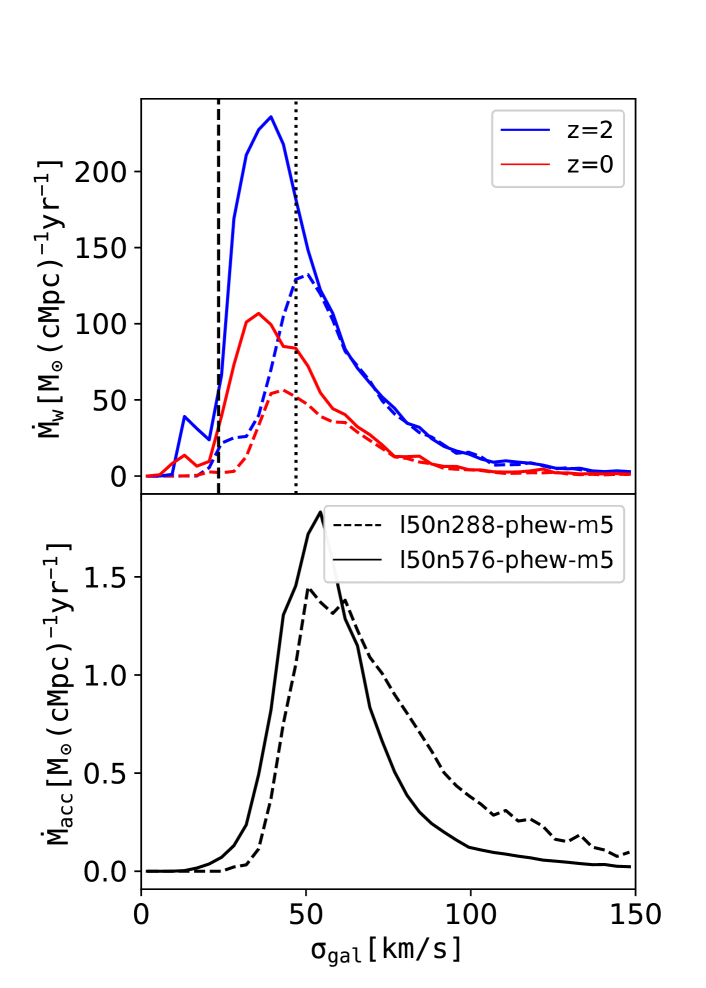
The top panel of Figure 14 compares the distribution of all winds that are launched from a simulation as a function of $\sigma_{\mathrm{gal}}$, which is the velocity dispersion of the haloes from which the winds are launched. It demonstrates that the high resolution simulation launches more than twice as much mass in winds as the low resolution simulation over time and that most of the extra winds are launched from the lowest mass haloes, i.e., smaller $\sigma_{\mathrm{gal}}$. Furthermore, above the resolution limit, both simulations launch nearly identical amount of winds from galaxies that are resolved in both simulations.

The lower panels of Figure 14 indicate where the accreted wind material originates in these two simulations. We select all wind material that recently accreted unto resolved galaxies (whose halo mass are larger than $10^{10}M_{\odot}$) within the last gigayear and show the distribution of $\sigma_{\mathrm{gal}}$ for where this wind material originates. It also demonstrates that the high resolution simulation not only launches more winds, but also that a considerable amount of this wind material is recycled.

6 Summary and Discussion

Modelling the interactions between galactic winds and their surrounding halo gas has been a challenge for cosmological simulations owing to the complicated interplay of physical processes that are unresolved in these simulations. In our previous paper (Huang et al., 2020b), we developed the Physically Evolved Winds (PhEW) model for analytically evolving cold galactic winds through an ambient medium. Our framework consistently models shocks, hydrodynamic instabilities, thermal conduction and evaporation, and makes predictions for the mass loss rate and the deceleration rate of the cloudlets that match the numerical results of high resolution cloud-crushing simulations from BS16 under various conditions.

In principle, a positive aspect of PhEW is that we can incorporate different models of the small scale physics, e.g., hydrodynamic instabilities, thermal conduction, shattering and entrainment. In this current work, the importance of hydrodynamic instabilities and thermal conduction are encapsulated in the parameters $f_{\mathrm{KH}}$ and $f_{\mathrm{s}}$, respectively. CGM observations could provide important constraints on the parameters, however, detailed comparisons with observations require additional post-processing steps, which we reserve for future work.

In this paper, we provide a detailed numerical prescription for implementing the PhEW model in cosmological hydrodynamic simulations. The PhEW model governs the evolution of the wind particles after they were launched from their host galaxies in a simulation. We performed several simulations with the PhEW model using various numerical and physical parameters to study the behaviours of the PhEW particles and their impact on the stellar and gas properties of the galaxies in the simulations.

The evolution of PhEW particles in our simulations strongly depends on halo mass. In low-mass haloes with $\log(M_{\mathrm{vir}}/M_{\odot})<11.5$, hydrodynamic instabilities dominate mass loss, even though most PhEW particles are still able to survive for hundreds of Megayears and escape their host haloes before they disintegrate. PhEW particles survive longest in intermediate-mass haloes with $\log(M_{\mathrm{vir}}/M_{\odot})\approx 12.0$, because weak thermal conduction can suppress hydrodynamic instabilities but still does not lead to efficient conductive evaporation. Some PhEW particles remain in the CGM/IGM even after a few gigayears. In the massive haloes with $\log(M_{\mathrm{vir}}/M_{\odot})>13.0$, the ambient halo gas becomes hot enough that strong thermal conduction leads to quick evaporation of the cloudlets, usually within 200 Megayears. Nevertheless, owing to the high initial speed of these winds, many particles can still travel a considerable distance, up to 0.5 $R_{\mathrm{vir}}$, before being fully evaporated.

The behaviour of PhEW particles is designed to be robust to numerical resolution and hydrodynamic technique (see appendix), in constrast to many other common galaxy supernova wind models (Katz et al., 1996; Springel & Hernquist, 2003; Oppenheimer & Davé, 2006; Stinson et al., 2006; Dalla Vecchia & Schaye, 2012; Agertz et al., 2013; Pillepich et al., 2018; Davé et al., 2019; Huang et al., 2020a), where wind properties may be more sensitive to resolution and to the complex interactions between resolution and the hydrodynamic technique. The PhEW wind behaviour does depend on the PhEW parameters, as it must, being based on an explicit model of the sub-grid physics. For example, a smaller cloudlet mass leads to cloudlets that disintegrate on shorter time-scales in both low-mass and massive haloes, although choosing a larger value for $f_{\mathrm{KH}}$ helps them to survive longer in low-mass haloes.

The evolution of wind particles and the galaxy properties in the PhEW simulations are much more robust to numerics than simulations without PhEW model. Between the gadget-3 and the gizmo simulations, which rely on different algorithms for solving hydrodynamics, the behaviours of wind particles are very different even with the same initial wind speeds and at the same resolution, with the winds in the gizmo simulation slowing down faster (see appendix). Furthermore, in both the SPH and the MFM method used by these simulations, the wind-halo interactions are unresolved and sensitive to numerical resolution. This leads to very different predictions on how far the winds can travel, the amount of wind recycling and the star formation histories of the galaxies. Because of this sensitivity of the wind model, one often needs to re-adjust the wind parameters for simulations with different resolutions to obtain similar results (Huang et al., 2020a). However, most results from the PhEW simulations converge very well at different resolutions without the need for wind retuning. We are hopeful that the PhEW model can be easily adapted to other cosmological hydrodynamic simulation codes whether they are Lagrangian, grid based, or moving mesh and still retain the numerical robustness that we demonstrated here.

Our results provide an initial view of how the sub-grid physics modelled by PhEW affects the evolution of galaxies, winds, and the CGM in simulations that are matched in numerical resolution, cooling and feedback physics, and the treatment of wind launch from galaxies. Our key findings are as follows.

1. At redshifts $z\geq 1$, the galaxy stellar mass function is little affected. However, at $z=0$ the mass function is boosted significantly below $M_{*}=10^{11}M_{\odot}$, achieving a better agreement with observations relative to equivalent simulations without the PhEW (e.g. Huang et al., 2020a). This change arises because there is much more wind recycling in these lower mass halos. This increase in recycling is caused by the ability of PhEW particles to shed some of their mass to the ambient CGM before escaping the halo, unlike traditional wind particles. This recycling leads to significantly better agreement with the empirically inferred stellar-to-halo mass relation at low redshift and thus with the observed galaxy stellar mass function. See Figures 7 and 8.

2. The high-mass end of the galaxy stellar mass function is minimally affected. In the absence of AGN feedback (or some other physics we have not included), simulations with or without PhEW produce excessively massive galaxies in large halos at low redshift, by about a factor of three at the highest masses. See Figure 7.

3. The CGM baryon fraction and the division of CGM baryons between cold and hot phases is only mildly affected. Across the halo mass range $10^{11}-10^{13}M_{\odot}$ the fraction of baryons in halos is depressed to 60-80% of the cosmic baryon fraction in our simulations, at $z=0$ and $z=2$, with or without PhEW. Cold CGM gas exceeds hot CGM gas in halos below $M_{h}\approx 10^{11.7}M_{\odot}$, and hot CGM gas exceeds cold CGM gas in halos above $10^{12}M_{\odot}$. Radial profiles of cold and hot CGM gas are also similar with or without PhEW. See Figure 9.

4. The distribution of metals in the CGM is radically affected because PhEW particles share metals with the ambient CGM as their clouds dissipate, while conventional wind particles retain their metals throughout. The distribution of CGM gas metallicities with PhEW is skewed but unimodal, while the conventional wind model gives a very broad and bimodal distribution. In our PhEW simulations the metallicity of hot CGM gas and cold CGM gas is similar, while our conventional wind simulations have a CGM comprised of metal-rich cold gas and metal-poor hot gas. See Figures 11 and 12.

Based on these exploratory results, we expect the change from a conventional wind implementation to PhEW to have an important impact on predictions for metal-line absorption and emission by the CGM, and perhaps on X-ray properties of galaxy halos, groups, and clusters. These changes arise from adopting a physically explicit model for dispersion of metals from winds to the ambient CGM, rather than a numerical prescription that is sensitive to resolution and to implementation details. We will examine predictions for these informative CGM and galaxy observables in future work.

Data availability

The data underlying this article will be shared on reasonable request to the corresponding author.

Appendix A A comparison between gadget and gizmo without PhEW

Simulations that use different numerical algorithms for solving hydrodynamic equations are known to produce different results in both high resolution simulations on small-scale hydrodynamic processes (Agertz et al., 2007; Hu et al., 2014; Hopkins, 2015) and in large-scale cosmological simulations (Frenk et al., 1999; Vogelsberger et al., 2012; Scannapieco et al., 2012; Sijacki et al., 2012; Nelson et al., 2013; Sembolini et al., 2016; Huang et al., 2019).

In this work we implement the PhEW model into gizmo and show how it affects the properties of galaxies and haloes in gizmo simulations. The gizmo MFM method solves hydrodynamics very differently from the gadget-3 (Springel, 2005) SPH method. Hopkins (2015) shows that the two algorithms produce different results in various standard hydrodynamic test problems. In addition, our version of gizmo also includes different cooling and star formation algorithms than we used in our gadget-3 simulations, as outlined in the main text. Hence, to isolate changes from our previous published simulations that owe to switching from our gadget-3 to our gizmo code, we evolved a non-PhEW simulation using our fiducial gadget-3 model (Huang et al., 2020a) to study how gizmo simulations compare to gadget-3 simulations using the same sub-grid wind model.

The purpose of the appendix is to show how the results from our PhEW simulations might compare to our published work using the gadget-3 code. The two codes are different in many aspects so the comparison is not meant to be a convergence study but rather to give an idea to the readers who are familiar with our previously published results how things might have changed with the new code.

This simulation, l50n288-gadget3, represents our previous simulations that model galactic winds with the sub-grid model of Huang et al. (2020a), and using our previous cooling and star formation algorithms. Here we use a version of the gadget-3 code (Huang et al., 2019) that employs the pressure-entropy SPH formulation (PE-SPH) (Hopkins, 2013), the Cullen & Dehnen (2010) artificial viscosity, artificial conduction (Price, 2008), and a time-step limiter (Durier & Dalla Vecchia, 2012). It models non-equilibrium cooling using the Wiersma et al. (2009) model and a Haardt & Madau (2012) UV background and models the interstellar medium and star formation using the effective equation of state model of Springel & Hernquist (2003) based on the observed Kennicutt (1998) relation.

In addition, we performed two simulations with gizmo using its implementation of the PE-SPH method instead of the MFM method, one without the PhEW (l50n288-phewoff-sph) and one with the PhEW (l50n288-phew-m5-sph). The PE-SPH method in the gizmo simulations also uses the Cullen & Dehnen (2010) artificial viscosity and artificial conduction as in the gadget-3 simulation. We use the same cooling and the star formation algorithms in these simulation as in the other gizmo simulations.

Figure 15: The galactic stellar mass functions at $z=0$. Here we compare the gadget-3 simulation (green) with several gizmo simulations, including the l50n288-phewoff (blue, MFM method without the PhEW model), the l50n288-phew-m5 (red, MFM method with the PhEW model), the l50n288-phewoff-sph (pink, PE-SPH method without the PhEW model) and the l50n288-phew-m5-sph simulation (red, PE-SPH method with the PhEW model). The results from the two simulations with the PhEW are close to each other, even though they use different hydrodynamic solvers, while the results from the three simulations without the PhEW are very different.

Figure 16: The composition of baryons in galactic haloes at $z=0$ similar to Figure 9. The dashed and solid lines indicate results from the gadget-3 simulations and the gizmo simulations, respectively. The shaded area corresponds to the 1$\sigma$ scatter from the gizmo simulation.

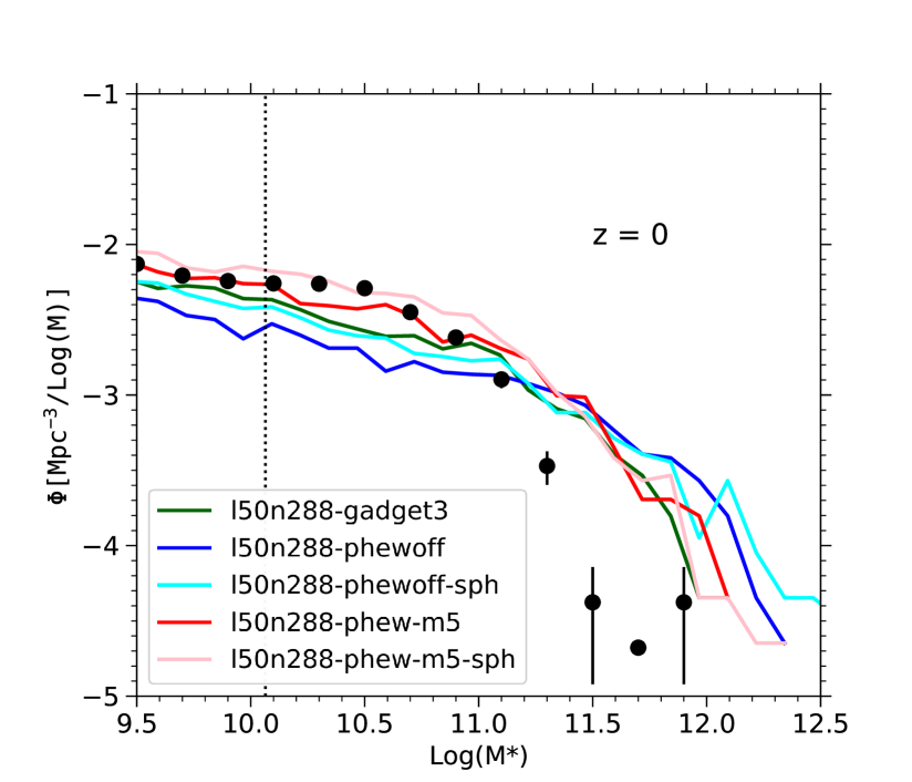
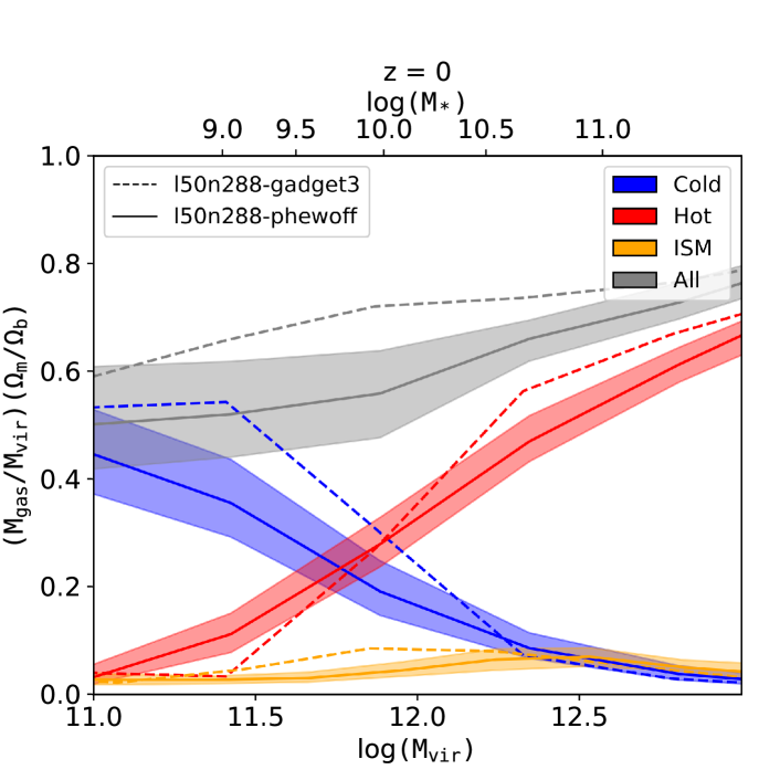
Figure 15 compares the $z=0$ GSMFs from these simulations. Their GSMFs at higher redshifts ($z\leqslant 1$) are similar to each other. We run all these simulations with the same initial density field but using different numerical methods for solving hydrodynamics, i.e. SPH methods implemented separately in gadget-3 and gizmo and the MFM method in gizmo. The GSMFs between the non-PhEW simulations (l50n288-gadget3, l50n288-phewoff and l50n288-phewoff-sph) are different over a wide range of masses. On the other hand, the GSMFs of the PhEW simulations are nearly identical with each other. This shows that when one changes the numerical hydrodynamic method or the numerical resolution in simulations using PhEW it only marginally affects the $z=0$ GSMF, again demonstrating the numerical robustness of PhEW. However, when using traditional wind propogation techniques, i.e. not using PhEW, there are significant differences in the results.

Figure 16 suggests that the cold and hot gas fractions between the two simulations are similar as well, except that the amount of cold gas is lower in the gizmo (l50n288-phewoff) simulation. These results are consistent with previous findings that the large scale properties of gas and stars from cosmological simulations are robust to changes in numerical algorithms even if they may have a large impact on small scale physics (Hu et al., 2014; Huang et al., 2019).

Figure 17: The same as Figure 4, except that we now compare the results from the gadget-3 (l50n288-gadget3) and the gizmo (l50n288-phewoff) simulations. Both simulations launch winds using the same sub-grid model, but the different hydrodynamics of the two simulations affect wind propagation very differently.

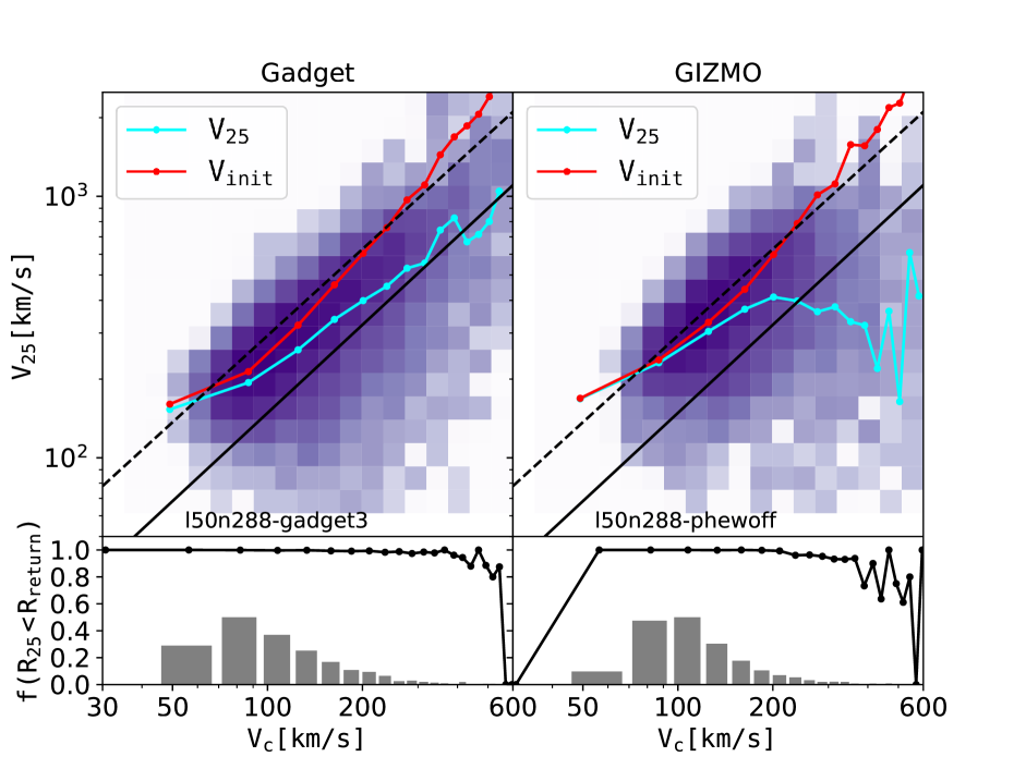
However, Figure 17 suggests that our gadget-3 versus gizmo simulations have strongly different dynamics, especially in massive haloes. If the different cooling and star formation physics between these two simulations has a minor impact on these dynamics, then the differing treatment of the underlying hydrodynamics may have a strong effect. Even though wind particles in both simulations have the same initial velocities at any given halo mass, those from the gizmo (l50n288-phewoff) simulation slow down faster than in the gadget-3 (l50n288-gadget3) simulation. As a result, wind particles become significantly slower in the gizmo (l50n288-phewoff) simulation at $0.25R_{\mathrm{vir}}$. Therefore, wind recycling is faster and more frequent in the gizmo (l50n288-phewoff) simulation, leading to more star formation in massive galaxies.

It is important to note, however, that neither gadget-3 nor gizmo actually resolves the small scale interactions between the winds and the surrounding gas, making the wind dynamics in both methods suspect and sensitive to both numerical resolution and numerical artefacts. In contrast, the PhEW model is very robust to both the numerical hydrodynamic algorithm and is almost independent of the numerical resolution.

References

- Agertz et al. (2007) Agertz O., et al., 2007, MNRAS, 380, 963
- Agertz et al. (2013) Agertz O., Kravtsov A. V., Leitner S. N., Gnedin N. Y., 2013, ApJ, 770, 25
- Anglés-Alcázar et al. (2017) Anglés-Alcázar D., Faucher-Giguère C.-A., Kereš D., Hopkins P. F., Quataert E., Murray N., 2017, MNRAS, 470, 4698
- Armillotta et al. (2016) Armillotta L., Fraternali F., Marinacci F., 2016, MNRAS, 462, 4157
- Asplund et al. (2009) Asplund M., Grevesse N., Sauval A. J., Scott P., 2009, ARA&A, 47, 481
- Behroozi et al. (2013) Behroozi P. S., Wechsler R. H., Conroy C., 2013, ApJ, 770, 57
- Brook et al. (2012) Brook C. B., et al., 2012, MNRAS, 426, 690
- Brook et al. (2014) Brook C. B., Stinson G., Gibson B. K., Shen S., Macciò A. V., Obreja A., Wadsley J., Quinn T., 2014, MNRAS, 443, 3809
- Brüggen & Scannapieco (2016) Brüggen M., Scannapieco E., 2016, ApJ, 822, 31
- Cottle et al. (2020) Cottle J., Scannapieco E., Brüggen M., Banda-Barragán W., Federrath C., 2020, ApJ, 892, 59
- Cullen & Dehnen (2010) Cullen L., Dehnen W., 2010, MNRAS, 408, 669
- Dalla Vecchia & Schaye (2008) Dalla Vecchia C., Schaye J., 2008, MNRAS, 387, 1431
- Dalla Vecchia & Schaye (2012) Dalla Vecchia C., Schaye J., 2012, MNRAS, 426, 140
- Davé et al. (2010) Davé R., Oppenheimer B. D., Katz N., Kollmeier J. A., Weinberg D. H., 2010, MNRAS, 408, 2051
- Davé et al. (2016) Davé R., Thompson R., Hopkins P. F., 2016, MNRAS, 462, 3265
- Davé et al. (2019) Davé R., Anglés-Alcázar D., Narayanan D., Li Q., Rafieferantsoa M. H., Appleby S., 2019, MNRAS, 486, 2827
- De Grandi & Molendi (2001) De Grandi S., Molendi S., 2001, ApJ, 551, 153
- Durier & Dalla Vecchia (2012) Durier F., Dalla Vecchia C., 2012, MNRAS, 419, 465
- Escala et al. (2018) Escala I., et al., 2018, MNRAS, 474, 2194
- Finlator et al. (2006) Finlator K., Davé R., Papovich C., Hernquist L., 2006, ApJ, 639, 672
- Ford et al. (2013) Ford A. B., Oppenheimer B. D., Davé R., Katz N., Kollmeier J. A., Weinberg D. H., 2013, MNRAS, 432, 89
- Ford et al. (2014) Ford A. B., Davé R., Oppenheimer B. D., Katz N., Kollmeier J. A., Thompson R., Weinberg D. H., 2014, MNRAS, 444, 1260
- Ford et al. (2016) Ford A. B., et al., 2016, MNRAS, 459, 1745
- Frenk et al. (1999) Frenk C. S., et al., 1999, ApJ, 525, 554
- Gabor & Davé (2012) Gabor J. M., Davé R., 2012, MNRAS, 427, 1816
- Gronke & Oh (2018) Gronke M., Oh S. P., 2018, MNRAS, 480, L111
- Haardt & Madau (2012) Haardt F., Madau P., 2012, ApJ, 746, 125
- Hafen et al. (2017) Hafen Z., et al., 2017, MNRAS, 469, 2292
- Hernquist & Katz (1989) Hernquist L., Katz N., 1989, ApJS, 70, 419
- Hirai & Saitoh (2017) Hirai Y., Saitoh T. R., 2017, ApJ, 838, L23
- Hopkins (2013) Hopkins P. F., 2013, MNRAS, 428, 2840
- Hopkins (2015) Hopkins P. F., 2015, MNRAS, 450, 53
- Hopkins et al. (2018) Hopkins P. F., et al., 2018, MNRAS, 480, 800
- Hu et al. (2014) Hu C.-Y., Naab T., Walch S., Moster B. P., Oser L., 2014, MNRAS, 443, 1173
- Huang et al. (2019) Huang S., et al., 2019, MNRAS, 484, 2021
- Huang et al. (2020a) Huang S., Katz N., Davé R., Oppenheimer B. D., Weinberg D. H., Fardal M., Kollmeier J. A., Peeples M. S., 2020a, MNRAS, 493, 1
- Huang et al. (2020b) Huang S., Katz N., Scannapieco E., Cottle J., Davé R., Weinberg D. H., Peeples M. S., Brüggen M., 2020b, MNRAS, 497, 2586
- Hummels et al. (2019) Hummels C. B., et al., 2019, ApJ, 882, 156
- Katz et al. (1996) Katz N., Weinberg D. H., Hernquist L., 1996, ApJS, 105, 19
- Kennicutt (1998) Kennicutt Jr. R. C., 1998, ApJ, 498, 541
- Kereš et al. (2005) Kereš D., Katz N., Weinberg D. H., Davé R., 2005, MNRAS, 363, 2
- Kereš et al. (2009) Kereš D., Katz N., Fardal M., Davé R., Weinberg D. H., 2009, MNRAS, 395, 160
- Kim & Ostriker (2015) Kim C.-G., Ostriker E. C., 2015, ApJ, 815, 67
- Kitayama & Suto (1996) Kitayama T., Suto Y., 1996, ApJ, 469, 480
- Krumholz & Gnedin (2011) Krumholz M. R., Gnedin N. Y., 2011, ApJ, 729, 36
- Leccardi & Molendi (2008) Leccardi A., Molendi S., 2008, A&A, 487, 461
- Lehner et al. (2013) Lehner N., et al., 2013, ApJ, 770, 138
- Li et al. (2019) Li Z., Hopkins P. F., Squire J., Hummels C., 2019, arXiv e-prints, p. arXiv:1909.02632
- Mandelker et al. (2019) Mandelker N., van den Bosch F. C., Springel V., van de Voort F., 2019, ApJ, 881, L20
- Marinacci et al. (2010) Marinacci F., Binney J., Fraternali F., Nipoti C., Ciotti L., Londrillo P., 2010, MNRAS, 404, 1464
- Martizzi et al. (2016) Martizzi D., Fielding D., Faucher-Giguère C.-A., Quataert E., 2016, MNRAS, 459, 2311
- McCourt et al. (2015) McCourt M., O’Leary R. M., Madigan A.-M., Quataert E., 2015, MNRAS, 449, 2
- McCourt et al. (2018) McCourt M., Oh S. P., O’Leary R., Madigan A.-M., 2018, MNRAS, 473, 5407
- McKee & Cowie (1975) McKee C. F., Cowie L. L., 1975, ApJ, 195, 715
- Molendi et al. (2016) Molendi S., Eckert D., De Grandi S., Ettori S., Gastaldello F., Ghizzardi S., Pratt G. W., Rossetti M., 2016, A&A, 586, A32
- Moster et al. (2018) Moster B. P., Naab T., White S. D. M., 2018, MNRAS, 477, 1822
- Muratov et al. (2015) Muratov A. L., Kereš D., Faucher-Giguère C.-A., Hopkins P. F., Quataert E., Murray N., 2015, MNRAS, 454, 2691
- Naab & Ostriker (2017) Naab T., Ostriker J. P., 2017, Annual Review of Astronomy and Astrophysics, 55, 59
- Nelson et al. (2013) Nelson D., Vogelsberger M., Genel S., Sijacki D., Kereš D., Springel V., Hernquist L., 2013, MNRAS, 429, 3353
- Oppenheimer & Davé (2006) Oppenheimer B. D., Davé R., 2006, MNRAS, 373, 1265
- Oppenheimer & Davé (2008) Oppenheimer B. D., Davé R., 2008, MNRAS, 387, 577
- Oppenheimer & Davé (2009) Oppenheimer B. D., Davé R., 2009, MNRAS, 395, 1875
- Oppenheimer et al. (2010) Oppenheimer B. D., Davé R., Kereš D., Fardal M., Katz N., Kollmeier J. A., Weinberg D. H., 2010, MNRAS, 406, 2325
- Oppenheimer et al. (2012) Oppenheimer B. D., Davé R., Katz N., Kollmeier J. A., Weinberg D. H., 2012, MNRAS, 420, 829
- Peeples et al. (2019) Peeples M. S., et al., 2019, ApJ, 873, 129
- Pilkington et al. (2012) Pilkington K., et al., 2012, MNRAS, 425, 969
- Pillepich et al. (2018) Pillepich A., et al., 2018, MNRAS, 473, 4077
- Price (2008) Price D. J., 2008, Journal of Computational Physics, 227, 10040
- Prochaska et al. (2017) Prochaska J. X., et al., 2017, ApJ, 837, 169
- Rennehan (2021) Rennehan D., 2021, arXiv e-prints, p. arXiv:2104.07673
- Revaz et al. (2016) Revaz Y., Arnaudon A., Nichols M., Bonvin V., Jablonka P., 2016, A&A, 588, A21
- Scannapieco & Brüggen (2015) Scannapieco E., Brüggen M., 2015, ApJ, 805, 158
- Scannapieco et al. (2012) Scannapieco C., et al., 2012, MNRAS, 423, 1726
- Schaye et al. (2015) Schaye J., et al., 2015, MNRAS, 446, 521
- Schneider & Robertson (2017) Schneider E. E., Robertson B. E., 2017, ApJ, 834, 144
- Sembolini et al. (2016) Sembolini F., et al., 2016, MNRAS, 459, 2973
- Shen et al. (2010) Shen S., Wadsley J., Stinson G., 2010, MNRAS, 407, 1581
- Sijacki et al. (2012) Sijacki D., Vogelsberger M., Kereš D., Springel V., Hernquist L., 2012, MNRAS, 424, 2999
- Smagorinsky (1963) Smagorinsky J., 1963, Monthly Weather Review, 91, 99
- Smith et al. (2017) Smith B. D., et al., 2017, MNRAS, 466, 2217
- Springel (2005) Springel V., 2005, MNRAS, 364, 1105
- Springel & Hernquist (2003) Springel V., Hernquist L., 2003, MNRAS, 339, 312
- Stinson et al. (2006) Stinson G., Seth A., Katz N., Wadsley J., Governato F., Quinn T., 2006, MNRAS, 373, 1074
- Su et al. (2017) Su K.-Y., Hopkins P. F., Hayward C. C., Faucher-Giguère C.-A., Kereš D., Ma X., Robles V. H., 2017, MNRAS, 471, 144
- Suresh et al. (2019) Suresh J., Nelson D., Genel S., Rubin K. H. R., Hernquist L., 2019, MNRAS, 483, 4040
- Tremmel et al. (2017) Tremmel M., Karcher M., Governato F., Volonteri M., Quinn T. R., Pontzen A., Anderson L., Bellovary J., 2017, MNRAS, 470, 1121
- Tumlinson et al. (2017) Tumlinson J., Peeples M. S., Werk J. K., 2017, ARA&A, 55, 389
- Vogelsberger et al. (2012) Vogelsberger M., Sijacki D., Kereš D., Springel V., Hernquist L., 2012, MNRAS, 425, 3024
- Wiersma et al. (2009) Wiersma R. P. C., Schaye J., Smith B. D., 2009, MNRAS, 393, 99
- Zhang et al. (2017) Zhang D., Thompson T. A., Quataert E., Murray N., 2017, MNRAS, 468, 4801
- van de Voort et al. (2019) van de Voort F., Springel V., Mandelker N., van den Bosch F. C., Pakmor R., 2019, MNRAS, 482, L85