Smooth Bilevel Programming
for Sparse Regularization

Abstract

Iteratively reweighted least square (IRLS) is a popular approach to solve sparsity-enforcing regression problems in machine learning. State of the art approaches are more efficient but typically rely on specific coordinate pruning schemes. In this work, we show how a surprisingly simple re-parametrization of IRLS, coupled with a bilevel resolution (instead of an alternating scheme) is able to achieve top performances on a wide range of sparsity (such as Lasso, group Lasso and trace norm regularizations), regularization strength (including hard constraints), and design matrices (ranging from correlated designs to differential operators). Similarly to IRLS, our method only involves linear systems resolutions, but in sharp contrast, corresponds to the minimization of a smooth function. Despite being non-convex, we show that there are no spurious minima and that saddle points are “ridable”, so that there always exists a descent direction. We thus advocate for the use of a BFGS quasi-Newton solver, which makes our approach simple, robust and efficient. We perform a numerical benchmark of the convergence speed of our algorithm against state of the art solvers for Lasso, group Lasso, trace norm and linearly constrained problems. These results highlight the versatility of our approach, removing the need to use different solvers depending on the specificity of the ML problem under study.

1 Introduction

Regularized empirical risk minimization is a workhorse of supervised learning, and for a linear model, it reads

$$\min_{\beta\in\mathbb{R}^{n}}R(\beta)+\frac{1}{\lambda}L(X\beta,y) \mathcal{P}_{\lambda}$$ ()

where $X\in\mathbb{R}^{m\times n}$ is the design matrix ($n$ being the number of samples and $m$ the number of features), $L:\mathbb{R}^{m}\times\mathbb{R}^{m}\to[0,\infty)$ is the loss function, and $R:\mathbb{R}^{n}\to[0,\infty)$ the regularizer. Here $\lambda\geqslant 0$ is the regularisation parameter which is typically tuned by cross-validation, and in the limit case $\lambda=0$, $(\mathcal{P}_{0})$ is a constraint problem $\min_{\beta}R(\beta)$ under the constraint $L(X\beta,y)=0$.

In this work, we focus our attention to sparsity enforcing penalties, which induce some form of structure on the solution of ($\mathcal{P}_{\lambda}$), the most celebrated examples (reviewed in Section 2) being the Lasso, group-Lasso and trace norm regularizers. All these regularizers, and much more (as detailed in Section), can be conveniently re-written as an infimum of quadratic functions. While Section 2 reviews more general formulations, this so-called “quadratic variational form” is especially simple in the case of block-separable functionals (such as Lasso and group-Lasso), where one has

$$R(\beta)=\min_{\eta\in\mathbb{R}^{k}_{+}}\frac{1}{2}\sum_{g\in\mathcal{G}}\frac{|\!|\beta_{g}|\!|_{2}^{2}}{\eta_{g}}+\frac{1}{2}h(\eta),$$ (1)

where $\mathcal{G}$ is a partition of $\{1,\ldots,n\}$, $k=|\mathcal{G}|$ is the number of groups and $h:\mathbb{R}^{k}_{+}\to[0,\infty)$. An important example is the group-Lasso, where $R(\beta)=\sum_{g}|\!|\beta_{g}|\!|_{2}$ is a group-$\ell_{1}$ norm, in which case $h(\eta)=\sum_{i}\eta_{i}$. The special case of the Lasso, corresponding to the $\ell_{1}$ norm is obtained when $g=\{i\}$ for $i=1,\ldots,n$ and $k=n$. This quadratic variational form (1) is at the heart of the Iterative Reweighted Least Squares (IRLS) approach, reviewed in Section 1.1. We refer to Section 2 for an in-depth exposition of these formulations.

Sparsity regularized problems ($\mathcal{P}_{\lambda}$) are notoriously difficult to solve, especially for small $\lambda$, because $R$ is a non-smooth function. It is the non-smoothness of $R$ which forces the solutions of ($\mathcal{P}_{\lambda}$) to belong to low-dimensional spaces (or more generally manifolds), the canonical example being spaces of sparse vectors when solving a Lasso problem. We refer to [3] for an overview of sparsity-enforcing regularization methods. The core idea of our algorithm is that a simple re-parameterization of (1) combined with a bi-level programming (i.e. solving two nested optimization problems) can turn ($\mathcal{P}_{\lambda}$) into a smooth program which is much better conditioned, and can be tackled using standard but highly efficient optimization techniques such as quasi-Newton (L-BFGS). Indeed, by doing the change of variable $(v_{g},u_{g})\triangleq(\sqrt{\eta_{g}},\beta_{g}/\sqrt{\eta_{g}})$ in (1), ($\mathcal{P}_{\lambda}$) is equivalent to

$$\min_{v\in\mathbb{R}^{k}}f(v)\quad\text{where}\quad f(v)\triangleq\min_{u\in\mathbb{R}^{n}}G(u,v)$$ (2)

$$G(u,v)\triangleq\frac{1}{2}h(v\odot v)+\frac{1}{2}|\!|u|\!|^{2}+\frac{1}{\lambda}L(X(v\odot_{\mathcal{G}}u),y).$$ (3)

Throughout, we define $\odot$ to be the standard Hadamard product and for $v\in\mathbb{R}^{k}$ and $u\in\mathbb{R}^{n}$, we define $v\odot_{\mathcal{G}}u\in\mathbb{R}^{n}$ to be such that $(v\odot_{\mathcal{G}}u)_{g}=v_{g}u_{g}$. Provided that $v\mapsto h(v\odot v)$ is differentiable and $L(\cdot,y)$ is a convex, proper, lower semicontinuous function, the inner minimisation problem has a unique solution and $f$ is differentiable. Moreover, in the case of the quadratic loss $L(z,y)\triangleq\frac{1}{2}|\!|z-y|\!|_{2}^{2}$, the gradient of $f$ can be computed in closed form, by solving a linear system of dimension $m$ or $n$. This paper is thus devoted to study the theoretical and algorithmic implications of this simple twist on the celebrated IRLS approach.

Comparison with proximal gradient

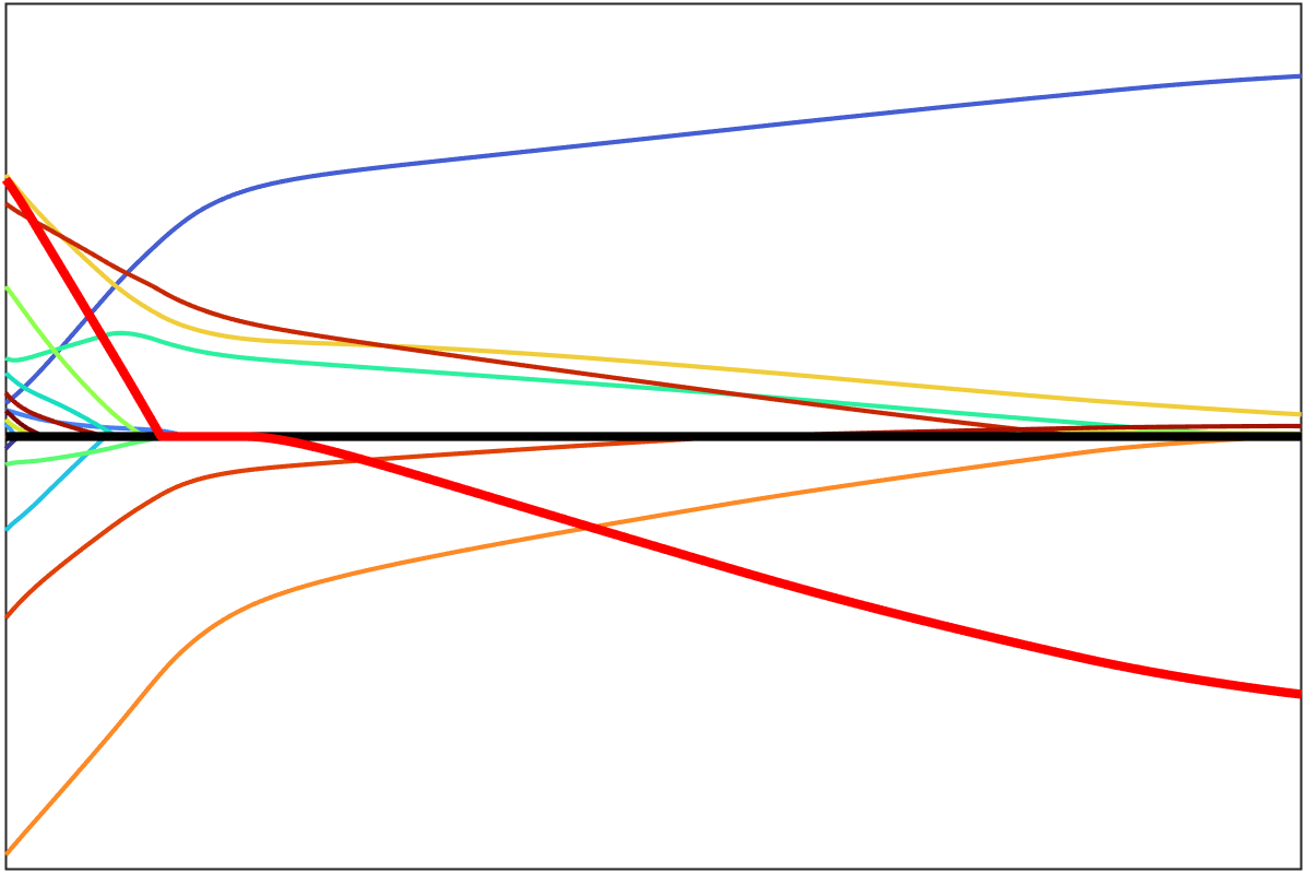
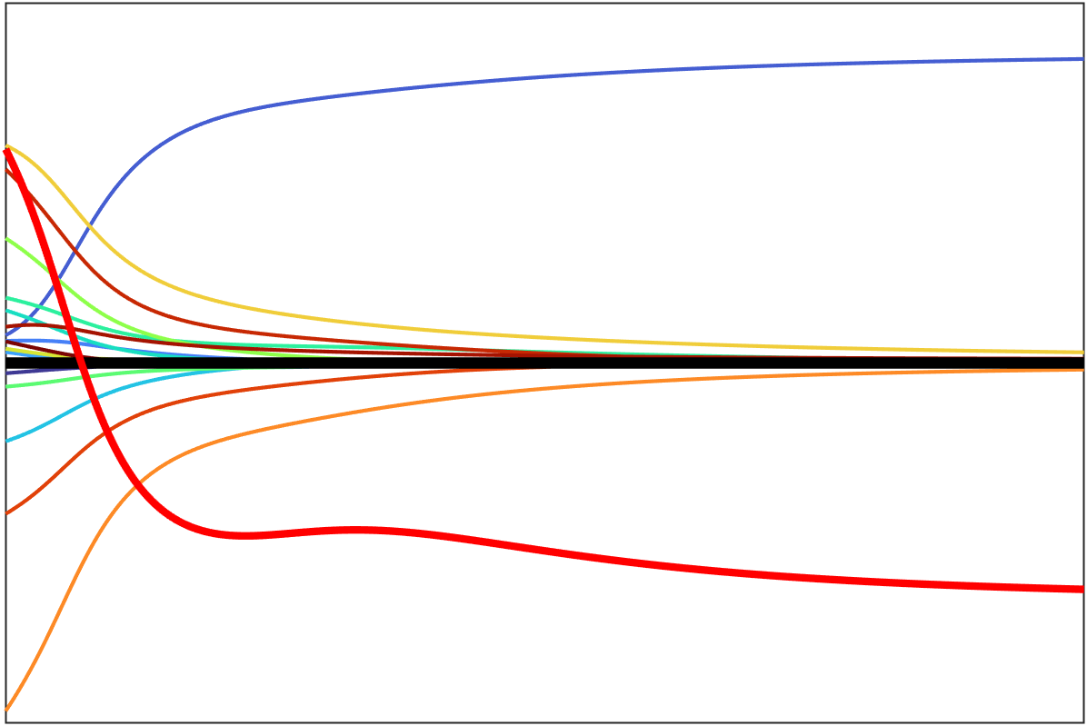
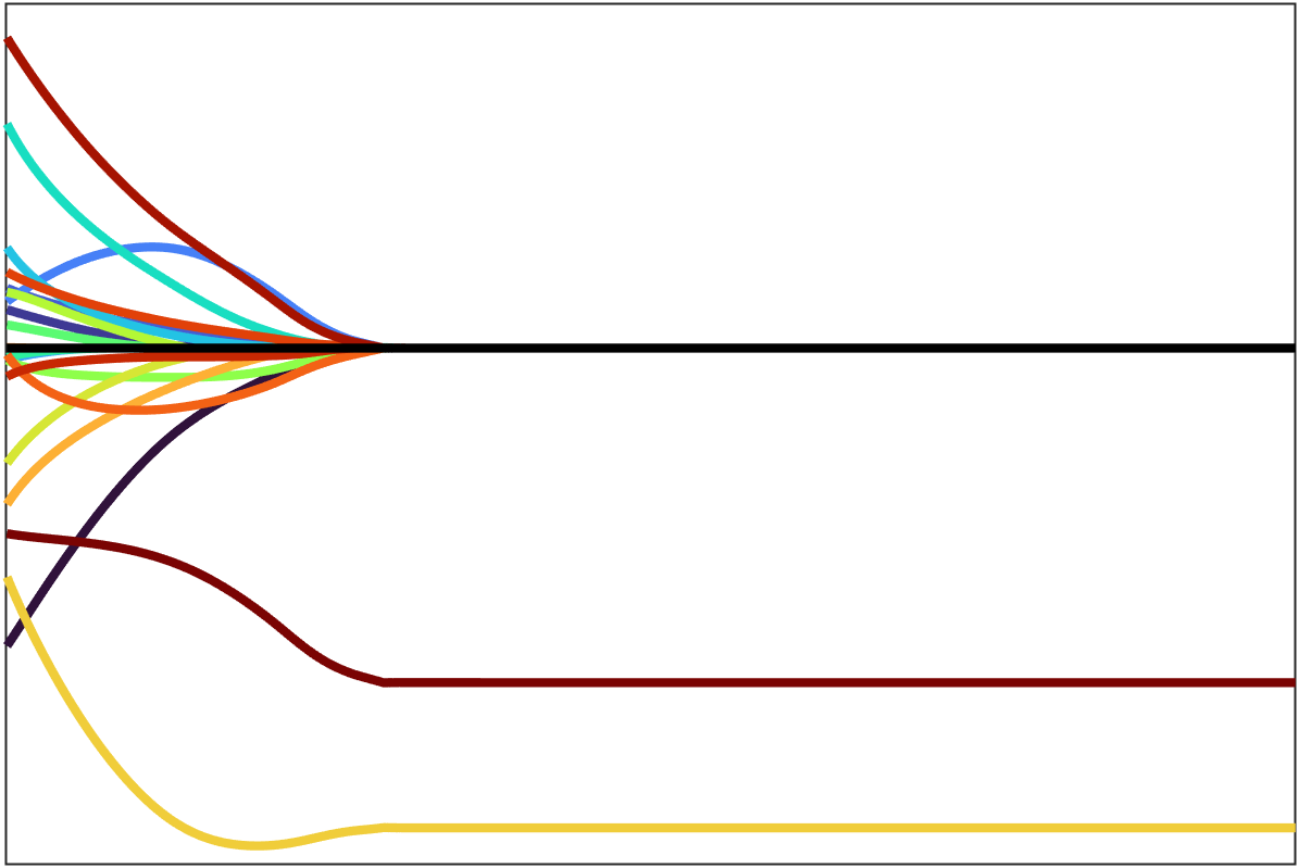
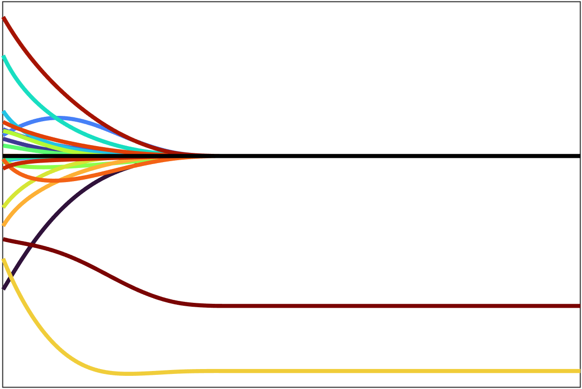
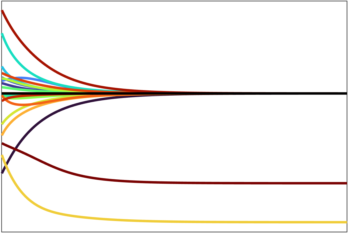
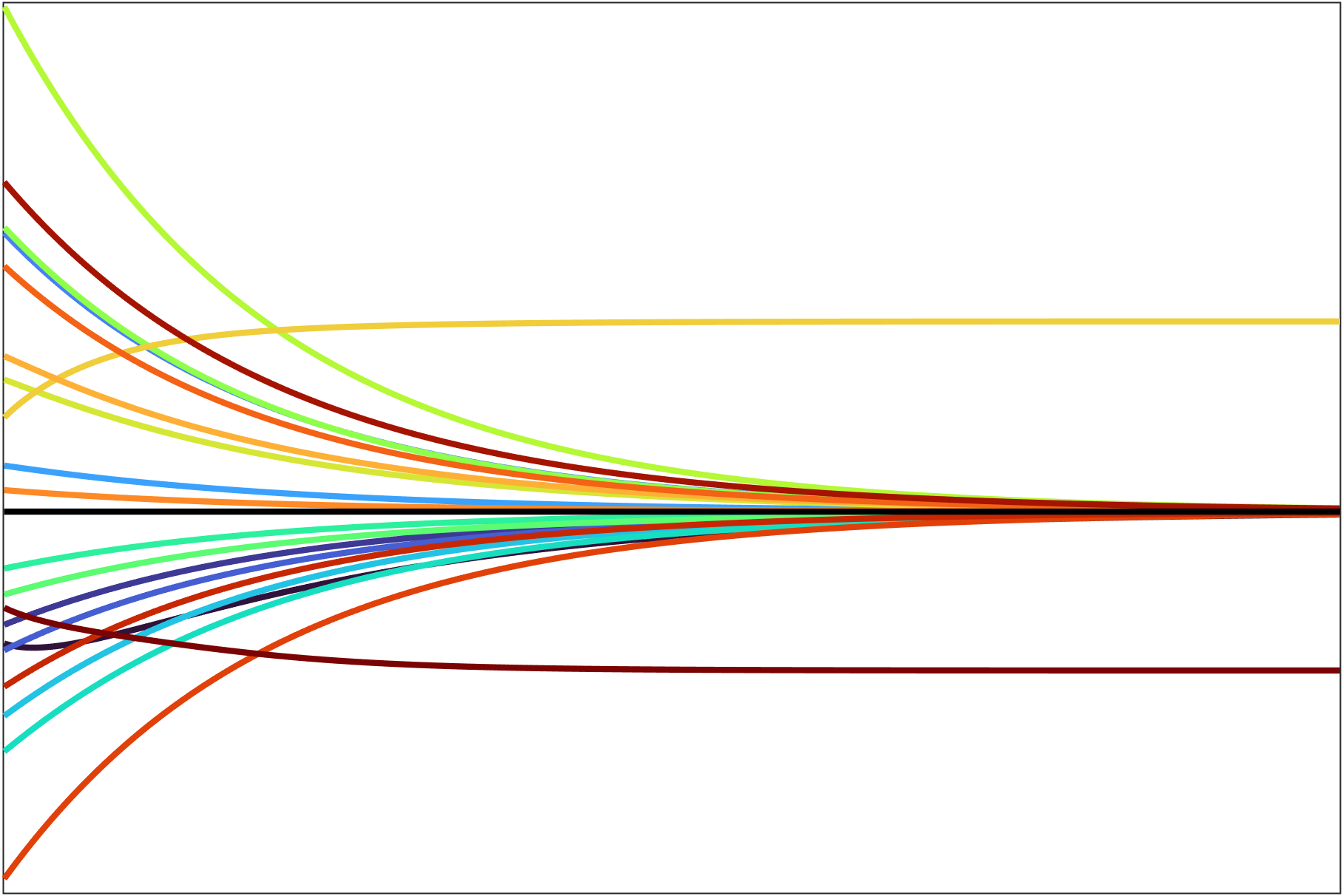
To provide some intuition about the proposed approach, Figure 1 contrasts the iterations of gradient descent on $f$ and of the iterative soft thresholding algorithm (ISTA) on the Lasso. We consider a random Gaussian matrix $X\in\mathbb{R}^{10\times 20}$ with $\lambda=|\!|X^{\top}y|\!|_{\infty}/10$. The ISTA trajectory is non-smooth when some feature crosses 0. In particular, if a coefficient (such as the red one on the figure) is initialized with the wrong sign, it takes many iterations for ISTA to flip sign. In sharp contrast, the gradient flow of $f$ does not exhibit such a singularity and exhibits smooth geometric convergence. We refer to the appendix for an analysis of this phenomenon.

ISTA

Noncvx-Pro

Figure 1: Evolution of 20 coefficients via ISTA and gradient descent of $f$.

Contributions

Our main contribution is a new versatile algorithm for sparse regularization, which applies standard smooth optimization methods to minimize the function $f$ in (2). We first propose in Section 2 a generic class of regularizers $R$ that enjoy a quadratic variational form. This section recaps existing results under a common umbrella and shows the generality of our approach. Section 3.1 then gathers the theoretical analysis of the method, and in particular the proof that while being non-convex, the function $f$ has no local minimum and only “ridable” saddle points. As a result, one can guarantee convergence to a global minimum for many optimisation schemes, such as gradient descent with random perturbations [36, 34] or trust region type methods [46]. Furthermore, for the case of the group Lasso, we show that $f$ is an infinitely differentiable function with uniformly bounded Hessian. Consequently, standard solvers such as Newton’s method/BFGS can be applied and with a superlinear convergence guarantee. Section 4 performs a detailed numerical study of the method and benchmarks it against several popular competing algorithms for Lasso, group-Lasso and trace norm regularization. Our method is consistently amongst the best performers, and is in particular very efficient for small values of $\lambda$, and can even cope with the constrained case $\lambda=0$.

1.1 Related works

State of the art solvers for sparse optimisation

Popular approaches to nonsmooth sparse optimisation include proximal based methods. The simplest instance is the Forward-Backward algorithm [37, 18] which handles the case where $L$ is a smooth function. There are many related inertial based acceleration schemes, such as FISTA [6] and particularly effective techniques that leads to substantial speedups are the adaptive use of stepsizes and restarting strategies [45]. Other related approaches are proximal quasi-Newton and variable metric methods [17, 7], which incorporate variable metrics into the quadratic term of the proximal operator. Another popular approach, particularly for the Lasso-like problems are coordinate descent schemes [23]. These schemes are typically combined with support pruning schemes [26, 42, 39]. In the case where both the regularisation and loss terms are nonsmooth (e.g. in the basis pursuit setting), typical solvers are the primal-dual [14], ADMM [11] and Douglas-Rachford algorithms [21]. Although these schemes are very popular due to their relatively low per iteration complexity, these methods have sublinear convergence rates in general, with linear convergence under strong convexity.

The quadratic variational formulation and IRLS

Quadratic variational formulations such as (1) have been exploited in many early computer vision works, such as [24] and [25]. One of the first theoretical results can be found in [25], see also [10] which lists many examples. Our result in Theorem 1 can be seen as a generalisation of these early works. Norm regularizers of this form were introduced in [40], and further studied in the monograph [3] under the name of subquadratic norms. The main algorithmic consequence of the quadratic variational formulation in the literature is the iterative reweighted least squares (IRLS) algorithm. When $L(z,y)=\frac{1}{2}|\!|z-y|\!|_{2}^{2}$ is the quadratic loss, a natural optimisation strategy is alternating minimising. However, due to the $1/\eta_{g}$ term, one needs to introduce some regularisation to ensure convergence. One popular approach is to add $\frac{\varepsilon}{2}\sum_{g}\eta_{g}^{-1}$ to the formulation (1) which leads to the IRLS algorithm [19]. The $\varepsilon$-term can be seen as a barrier to keep $\eta_{g}$ positive which is reminiscent of interior point methods. The idea of IRLS is to do alternating minimisation over $\beta$ and $\eta$, where the minimisation with respect to $\beta$ is a least squares problem, and the minimisation with respect to $\eta$ admits a closed form solution. A nuclear norm version of IRLS has been used in [1] where an alternating minimisation algorithm was introduced. Finally, we remark that although nonconvex formulations for various low complexity regularizers have appeared in the literature, see for instance [50, 31, 38, 32] for the case of the $\ell_{1}$ and nuclear norms, they are typically associated with alternating minimisation algorithms.

Variable projection/reduced gradient approaches

IRLS methods are quite slow because the resulting minimization problem is poorly conditioned. Adding the smoothing term $\frac{\varepsilon}{2}\sum_{g}\eta_{g}^{-1}$ only partly alleviates this, and also breaks the sparsity enforcing property of the regularizer $R$. We avoid both issues in (2) by solving a “reduced” problem which is much better conditioned and smooth. This idea of solving a bi-variate problem by re-casting it as a bilevel program is classical, we refer in particular to [51, Chap. 10] for some general theoretical results on reduced gradients, and also Danskin’s theorem (although this is restricted to the convex setting) in [8]. Our formulation falls directly into the framework of variable projection [52, 28], introduced initially for solving nonlinear least squares problems. Properties and advantages of variable projection have been studied in [52], we refer also to [33, 59] for more recent studies. Nonsmooth variable projection is studied in [57], although the present work is in the classical setting of variable projection due to our smooth reparametrization. Reduced gradients have also been associated with the quadratic variational formulation in several works [3, 48, 49]. The idea is to apply descent methods over $g(\eta)=\min_{\beta}R_{0}(\eta,\beta)+\frac{1}{2}|\!|X\beta-y|\!|_{2}^{2}$. Although the function over $\eta$ and $\beta$ is discontinuous, the function $g$ over $\eta$ is smooth and one can apply first order methods, such as proximal gradient descent to minimise $g$ under positivity constraints. While quasi-Newton methods can be applied in this setting with bound constraints, we show in Section 4.1 that this approach is typically less effective than our nonconvex bilevel approach. In the setting of the trace norm, the optimisation problem is constrained on the set of positive semidefinite matrices, so one is restricted to using first order methods [48].

2 Quadratic variational formulations

We describe in this section some general results about when a regulariser has a quadratic variational form. Our first result brings together results which are scattered in the literature: it is closely related to Theorem 1 in [25], but their proof was only for strictly concave differentiable functions and did not explicitly connect to convex conjugates, while the setting for norms have been characterized in the monograph [3] under the name of subquadratic norms.

Theorem 1.

Let $R:\mathbb{R}^{n}\to\mathbb{R}$. The following are equivalent:
 (i) $R(\beta)=\varphi(\beta\odot\beta)$ where $\varphi$ is proper, concave and upper semi-continuous, with domain $\mathbb{R}_{+}^{d}$.
 (ii) There exists a convex function $\psi$ for which $R(\beta)=\inf_{z\in\mathbb{R}^{n}_{+}}\frac{1}{2}\sum_{i=1}^{n}z_{i}\beta_{i}^{2}+\psi(z)$.
Furthermore, $\psi(z)=(-\varphi)^{*}(-z/2)$ is defined via the convex conjugate $(-\varphi)^{*}$ of $-\varphi$, leading to (1) using the change of variable $\eta\leftarrow 1/z$ and $h(\eta)=2\psi(1/\eta)$. When $R$ is a norm, the function $h$ can be written in terms of the dual norm $R^{*}$ as $h(\eta)=\max_{R^{*}(w)\leqslant 1}\sum_{i}w_{i}^{2}\eta_{i}$. Moreover, $R(\beta)^{2}=\inf_{\eta\in\mathbb{R}^{n}_{+}}\left\{\sum_{i}{\beta_{i}^{2}}\eta_{i}^{-1}\;\backslash\;h(\eta)\leqslant 1\right\}$.

See Appendix B for the proof to this Theorem. Some additional properties of $\psi$ are derived in Lemma 1 of Appendix B, one property is that if $R$ is coercive, then $\lim_{|\!|z|\!|\to 0}\psi(z)=+\infty$, so the function $f$ is coercive (see also remark 2).

2.1 Examples

Let us first give some simple examples of both convex and non-convex norms:

1. Euclidean norms: for $R=|\!|\cdot|\!|_{2}$, making use of $R^{*}$ as stated in Theorem 1, one has $h=|\!|\cdot|\!|_{\infty}$.

2. Group norms: for $\mathcal{G}$ is a partition of $\{1,\ldots,n\}$, the group norm is $R(\beta)=\sum_{g\in\mathcal{G}}|\!|\beta_{g}|\!|$. Using the previous result for the Euclidean norm, one has $h(\eta)=\sum_{g\in\mathcal{G}}|\!|(\eta_{i})_{i\in g}|\!|_{\infty}$. This expression can be further simplified to obtain (1) with a reduced vector $\eta$ in $\mathbb{R}^{|\mathcal{G}|}_{+}$ in place of $\mathbb{R}^{n}$ by noticing that the optimal $\eta$ is constant in each group $g$.

3. $\ell^{q}$ (quasi) norms: For $R(\beta)=|\beta|^{q}$ where $q\in(0,2)$, one has $\varphi(u)={u}^{q/2}$ and one verifies that $h(\eta)=C_{q}\eta^{\frac{q}{2-q}}$ where $C_{q}=(2-q)q^{q/(2-q)}$. Note that for $q>\frac{2}{3}$, $v\mapsto h(v^{2})=v^{\gamma}$ for $\gamma>1$ is differentiable. Analysis and numerics for this nonconvex setting can be found in Appendix F.

Matrix regularizer

The extension of Theorem 1 to the case where $\beta=B$ is a matrix can be found in the appendix. When $R=\varphi(BB^{\top})$ is a function on matrices, the analogous quadratic variational formulation is

$$R(B)=\min_{Z\in\mathbb{S}^{n}_{+}}\min_{B\in\mathbb{R}^{n\times r}}\frac{1}{2}\sum_{g}\operatorname{tr}(B^{\top}Z^{-1}B)+\frac{1}{2}h(Z),$$ (4)

where $\mathbb{S}^{n}_{+}$ denotes the set of symmetric positive semidefinite matrices and $h(Z)=2(-\varphi)^{*}(-Z^{-1}/2)$. Letting $U=Z^{-1/2}B$ and $V=Z^{1/2}$, we have $B=VU$ and the equivalence

$$\min_{B}R(B)+\frac{1}{2\lambda}|\!|\mathcal{A}(B)-y|\!|_{2}^{2}$$ (5)

$$=\min_{V\in\mathbb{R}^{n\times n}}f(V)\triangleq\min_{U\in\mathbb{R}^{n\times r}}\frac{1}{2}|\!|U|\!|_{F}^{2}+\frac{1}{2}h(V^{\top}V)+\frac{1}{2\lambda}|\!|\mathcal{A}(VU)-y|\!|_{2}^{2}.$$ (6)

where $\mathcal{A}:\mathbb{R}^{n\times r}\to\mathbb{R}^{m}$ is a linear operator. Again, provided that $V\mapsto h(V^{\top}V)$ is differentiable, $f$ is a differentiable function with $\nabla f(V)=V\partial h(V^{\top}V)+\frac{1}{\lambda}\mathcal{A}^{*}(\mathcal{A}(VU)-y))U^{\top}$ and $U$ such that $\lambda U+V^{\top}\mathcal{A}^{*}(\mathcal{A}(VU)-y)=0$. For the trace norm, $R(B)=\operatorname{tr}(\sqrt{B^{\top}B})$, we have $h(Z)=\operatorname{tr}(Z)$ and $\partial h(Z)=\mathrm{Id}$. Note that, just in the vectorial case, one could write the inner minimisation problem over the dual variable $\alpha\in\mathbb{R}^{m}$ and handle the case of $\lambda=0$.

3 Theoretical analysis

Our first result shows the equivalence between ($\mathcal{P}_{\lambda}$) and a smooth bilevel problem.

Theorem 2.

Denote $L_{y}\triangleq L(\cdot,y)$ and let $L_{y}^{*}$ denote the convex conjugate of $L_{y}$. Assume that $L_{y}$ is a convex, proper, lower semicontinuous function and $R$ takes the form (1). The problem ($\mathcal{P}_{\lambda}$) is equivalent to

$$\min_{v\in\mathbb{R}^{k}}f(v) \triangleq\min_{u\in\mathbb{R}^{n}}\frac{1}{2}h(v\odot v)+\frac{1}{2}|\!|u|\!|^{2}+\frac{1}{\lambda}L_{y}\left(X(v\odot_{\mathcal{G}}u)\right).$$ (7)

$$=\max_{\alpha\in\mathbb{R}^{m}}\frac{1}{2}h(v\odot v)-\frac{1}{\lambda}L_{y}^{*}\left(\lambda\alpha\right)-\frac{1}{2}|\!|v\odot_{\mathcal{G}}(X^{\top}\alpha)|\!|_{2}^{2}.$$ (8)

where $v\odot_{\mathcal{G}}u\triangleq(u_{g}v_{g})_{g\in\mathcal{G}}$. The minimiser $\beta$ to ($\mathcal{P}_{\lambda}$) and the minimiser $v$ to (7) are related by $\beta=v\odot_{\mathcal{G}}u=-v^{2}\odot_{\mathcal{G}}X^{\top}\alpha.$ Provided that $v\mapsto h(v\odot v)$ is differentiable, the function $f$ is differentiable with gradient

$$\nabla f(v)=v\odot\partial h(v^{2})-v\odot_{\mathcal{G}}\left(|\!|X_{g}^{\top}\alpha|\!|^{2}\right)_{g}\quad\text{where}\quad\alpha\in\operatorname{argmax}_{\tilde{\alpha}}-L_{y}^{*}(\tilde{\alpha})-\frac{1}{2}|\!|v\odot_{\mathcal{G}}(X^{\top}\tilde{\alpha})|\!|_{2}^{2}.$$ (9)

Note that $\nabla f$ is uniquely defined even if $\alpha$ is not unique. If $\lambda>0$ and $L_{y}$ is differentiable, then we have the additional formula, with $u\in\operatorname{argmin}_{\tilde{u}}\frac{1}{2}|\!|\tilde{u}|\!|_{2}^{2}+\frac{1}{\lambda}L_{y}(X(v\odot_{\mathcal{G}}\tilde{u}))$,

$$\nabla f(v)=v\odot\partial h(v^{2})+\frac{1}{\lambda}\left(\langle u_{g},\,X_{g}^{\top}\partial L_{y}(X(v\odot_{\mathcal{G}}u)\rangle\right)_{g\in\mathcal{G}}.$$ (10)

Proof.

The equivalence between ($\mathcal{P}_{\lambda}$) and (7) is simply due to the quadratic variational form of $R$, and the change of variable $v_{g}=\sqrt{\eta_{g}}$, and $u_{g}=\beta_{g}/\sqrt{\eta_{g}}$. The equivalence to (8) follows by convex duality on the inner minimisation problem, that is

$$f(v) =\min_{u}G_{1}(v,u)\triangleq\frac{1}{2}h(v^{2})+\frac{1}{2}|\!|u|\!|^{2}+\frac{1}{\lambda}L_{y}(X(v\odot_{\mathcal{G}}u))$$

$$=\min_{u,z}\frac{1}{2}h(v^{2})+\frac{1}{2}|\!|u|\!|^{2}+\frac{1}{\lambda}L_{y}(z)\quad\text{where}\quad z=X(v\odot_{\mathcal{G}}u)$$

$$=\min_{u,z}\max_{\alpha}\frac{1}{2}h(v^{2})+\frac{1}{2}|\!|u|\!|^{2}+\frac{1}{\lambda}L_{y}(z)-\langle\alpha,\,z\rangle+\langle\alpha,\,X(v\odot_{\mathcal{G}}u)\rangle$$

$$=\max_{\alpha}\min_{u}\frac{1}{2}h(v^{2})+\frac{1}{2}|\!|u|\!|^{2}+\langle\alpha,\,X(v\odot_{\mathcal{G}}u)\rangle-\frac{1}{\lambda}L_{y}^{*}(\lambda\alpha).$$

Using the optimality condition over $u$, we obtain $u=-v\odot_{\mathcal{G}}X^{\top}\alpha$ and hence,

$$f(v)=\max_{\alpha}G_{2}(v,\alpha)\triangleq\frac{1}{2}h(v^{2})-\frac{1}{2}|\!|v\odot_{\mathcal{G}}X^{\top}\alpha|\!|^{2}_{2}-\frac{1}{\lambda}L_{y}^{*}(\lambda\alpha).$$

By [51, Theorem 10.58], if the following set

$$\mathcal{S}(v)\triangleq\left\{\partial_{v}G_{2}(v,\alpha)=v-v\odot_{\mathcal{G}}(|\!|X_{g}^{\top}\alpha|\!|^{2}_{2})_{g\in\mathcal{G}}\;\backslash\;\alpha\in\operatorname{argmin}_{\alpha}G_{2}(v,\alpha)\right\}$$

is singled valued, then $f$ is differentiable with $\nabla f(v)=\partial_{v}G_{2}(v,\alpha)$ for $\alpha\in\operatorname{argmin}_{\alpha}G_{2}(v,\alpha)$. Observe that even if $\operatorname{argmin}_{\alpha}G_{2}(v,\alpha)$ is not single valued, since $G_{2}$ is strongly convex for $v\odot_{\mathcal{G}}X^{\top}\alpha$, $\mathcal{S}(v)$ is single-valued and hence, $f$ is a differentiable function.

In the case where $L_{y}$ is differentiable, we can again apply [51, Theorem 10.58], to obtain $\nabla f(v)=v\odot\partial h(v^{2})+\partial_{v}G_{1}(v,y)$ with $u=\operatorname{argmin}_{u}G_{1}(v,u)$ (noting that $G_{1}(v,\cdot)$ is strongly convex and has a unique minimiser) which is precisely the gradient formula (10).

∎

For the Lasso and basis pursuit setting, the gradient of $f$ can be computed in closed form:

Corollary 1.

If $R$ has a quadratic variational form and $L_{y}(z)=\frac{1}{2}|\!|z-y|\!|_{2}^{2}$, then $\partial L_{y}(z)=z-y$, $L_{y}^{*}(\alpha)=\langle y,\,\alpha\rangle+\frac{1}{2}|\!|\alpha|\!|_{2}^{2}$ and the gradient of $f$ can be written as in (9) and additionally (10) when $\lambda>0$. Furthermore, $\alpha\in\mathbb{R}^{m}$ in (9) and $u\in\mathbb{R}^{n}$ in (10) solves

$$(X\operatorname{diag}(\bar{v}^{2})X^{\top}+\lambda\mathrm{Id})\alpha=-y,\quad\text{and}\quad(\operatorname{diag}(\bar{v})X^{\top}X\operatorname{diag}(\bar{v})+\lambda\mathrm{Id})u=v\odot_{\mathcal{G}}(X^{\top}y),$$ (11)

where $\bar{v}\in\mathbb{R}^{n}$ is defined as $\bar{v}\odot u=(v_{g}u_{g})_{g\in\mathcal{G}}$ for all $u\in\mathbb{R}^{n}$ and $\mathrm{Id}$ denotes the identity matrix.

This shows that our method caters for the case $\lambda=0$ with the same algorithm in a seamless manner. This is unlike most existing approach which work well for $\lambda>0$ (and typically do not require matrix inversion) but fails when $\lambda$ is small, whereas solvers dedicated for $\lambda=0$ might require inverting a linear system, see Section 4.4 for an illustrative example.

3.1 Properties of the projected function $f$

In this section, we analyse the case of the group Lasso. The following theorem ensures that the projected function $f$ has only strict saddle points or global minima. We say that $v$ is a second order stationary point if $\nabla f(v)=0$ and $\nabla^{2}f(v)\succeq 0$. We say that $v$ is a strict saddle point (often called “ridable”) if it is a stationary point but not a second order stationary point. One can thus always find a direction of descent outside the set of global minimum. This can be exploited to derive convergence guarantees to second order stationary points for trust region methods [46] and gradient descent methods [36, 34].

Theorem 3.

In the case $h(z)=\sum_{i}z_{i}$ and $L(z,y)=\frac{1}{2}|\!|z-y|\!|_{2}^{2}$, the projected function $f$ is infinitely continuously differentiable and for $v\in\mathbb{R}^{k}$, $\nabla f(v)=v\odot\left(1-|\xi|^{2}\right)$ where $\xi_{g}=\frac{1}{\lambda}X_{g}^{\top}(X(u\odot v)-y)$ and $u$ solves the inner least squares problem for $v$. Let $J$ denote the support of $v$, by rearranging the columns and rows, the Hessian of $f$ can be written as the following block diagonal matrix

$$\nabla^{2}f(v)=\begin{pmatrix}\operatorname{diag}(1-|\!|\xi_{g}|\!|_{2}^{2})_{g\in J}+4U^{\top}WU&0\\ 0&\operatorname{diag}(1-|\!|\xi_{g}|\!|_{2}^{2})_{g\in J^{c}}\end{pmatrix}$$ (12)

where $W\triangleq\mathrm{Id}-\lambda\left((v_{g}X_{g}^{\top}X_{h}v_{h})_{g,h\in J}+\lambda\mathrm{Id}_{J}\right)^{-1}$ and $U$ is the block diagonal matrix with blocks $(\xi_{g})_{g\in J}$, with $\max_{g\in\mathcal{G}}|\!|\xi_{g}|\!|_{2}\leqslant C$ and ${|\!|\nabla^{2}f(v)|\!|}\leqslant 1+3C^{2}$ where $C\triangleq{|\!|y|\!|_{2}}\max_{g\in\mathcal{G}}|\!|X_{g}|\!|/\lambda$. Moreover, all stationary points of $f$ are either global minima or strict saddles. At stationary points, the eigenvalues of the Hessian of $f$ are at most $4$ and is at least

$$\min\left(4(1-\lambda/(\lambda+\hat{\sigma})),\min_{g\not\in J}(1-|\!|\xi_{g}|\!|^{2})\right)$$

where $\hat{\sigma}$ is the smallest eigenvalue of $(v_{g}X_{g}^{\top}X_{h}v_{h})_{g,h\in J}$.

The proof can be found in Appendix C. We simply mention here that by examining the first order condition of ($\mathcal{P}_{\lambda}$), we see that $\beta$ is a minimizer if and only if $\xi$ satisfies $-\xi_{g}=\frac{\beta_{g}}{|\!|\beta_{g}|\!|_{2}}$ for all $g\in\operatorname{Supp}(\beta)$ and $|\!|\xi_{g}|\!|_{2}\leqslant 1$ for all $g\in\mathcal{G}$. The first condition on the support of $\beta$ is always satisfied at stationary points of the nonconvex function (2), and by examining (12), the second condition is also satisfied unless the stationary point is strict.

Remark 1 (Example of strict saddle point for our $f$).

One can observe that $v=0$ is a strict saddle point, as the solution to the associated linear system yields $u=0$ and hence $\nabla f(v)=0$. If $\lambda\geqslant|\!|X^{\top}y|\!|_{\infty}$, then $u=v=0$ corresponds to a global minimum, otherwise, it is clear to see that there exists $g$ such that $1-|\!|\xi_{g}|\!|^{2}<0$ and $v=0$ is a strict saddle point.

Remark 2.

Since $f\in C^{\infty}$, it is Lipschitz smooth on any bounded domain. As mentioned, $f$ is coercive when $R$ is coercive, and hence, its sublevel sets are bounded. So, for any descent algorithm, we can apply results based on $\nabla^{k}f$ being Lipschitz smooth for all $k$.

Remark 3.

The nondegeneracy condition that $|\!|\xi_{g}|\!|_{2}<1$ outside the support of $v$ and invertibility of $(X_{g}^{\top}X_{h})_{g,h\in J}$ is often used to derive consistency results [4, 62]. By Proposition 1, we see that this condition guarantees that the Hessian of $f$ is positive definite at the minimum, and hence, combining with the smoothness properties of $f$ explained in the previous remark, BFGS is guaranteed to converge superlinearly for starting points sufficiently close to the optimum [43, Theorem 6.6].

4 Numerical experiments

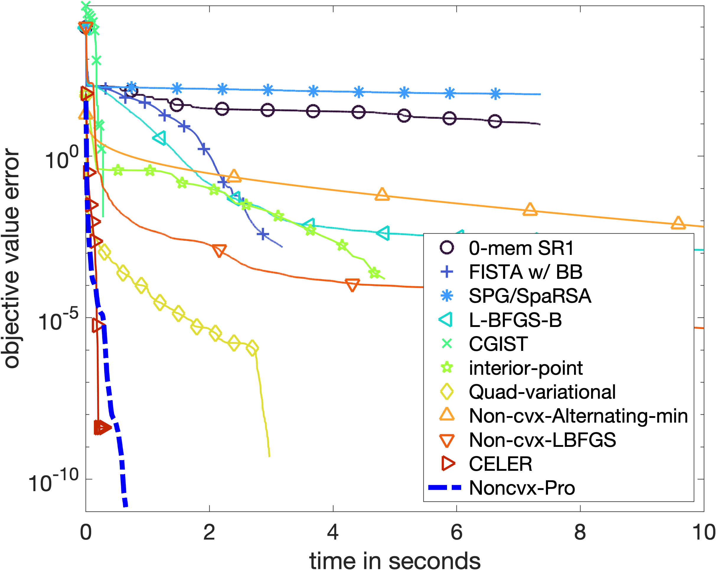
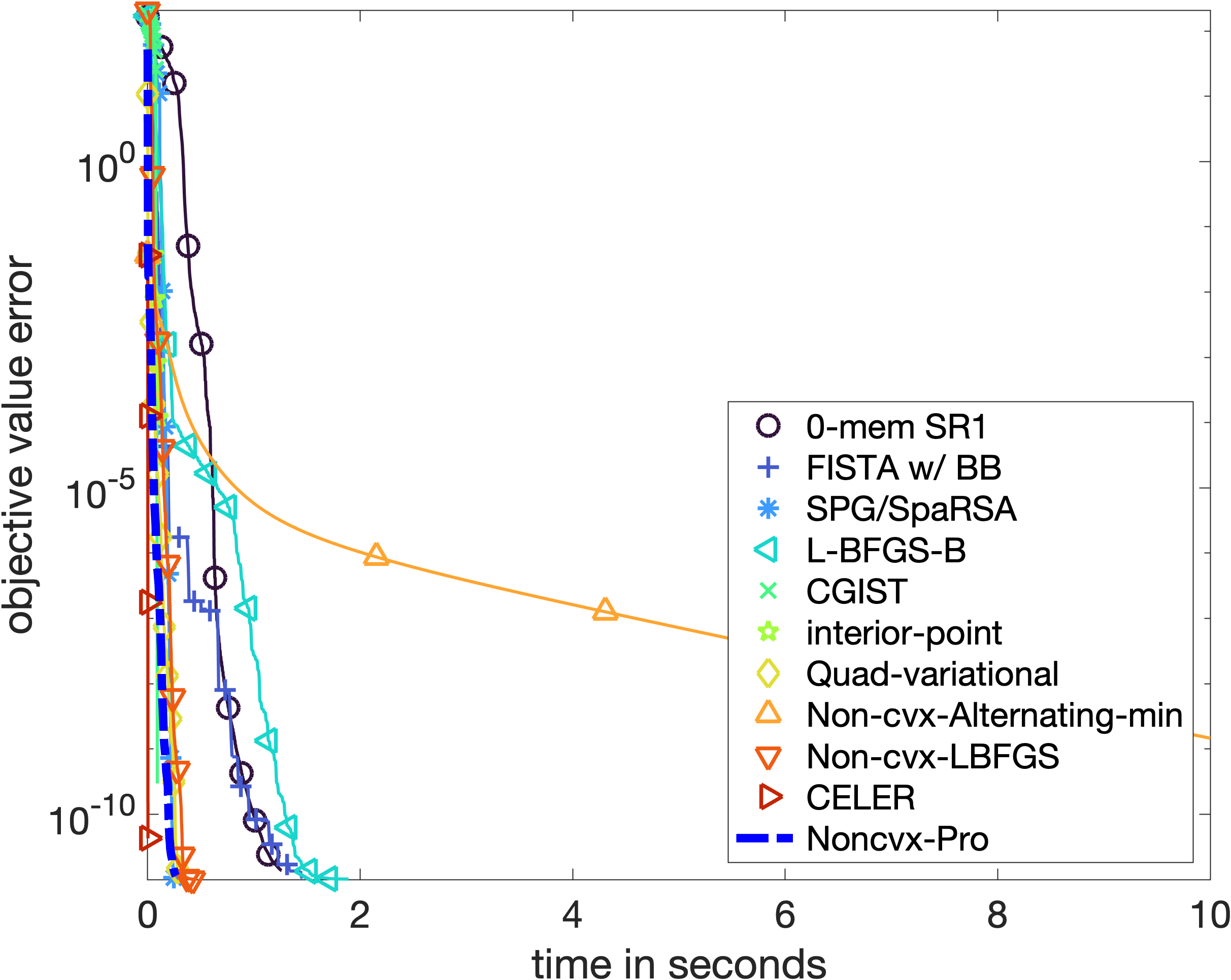
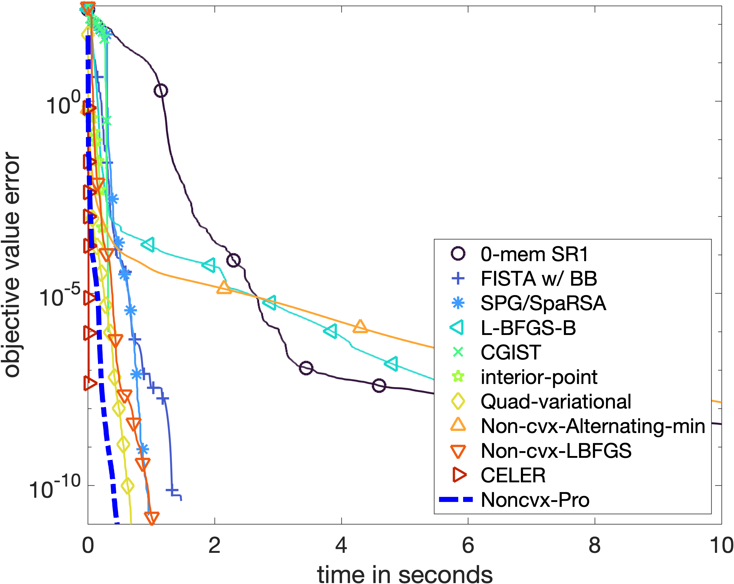
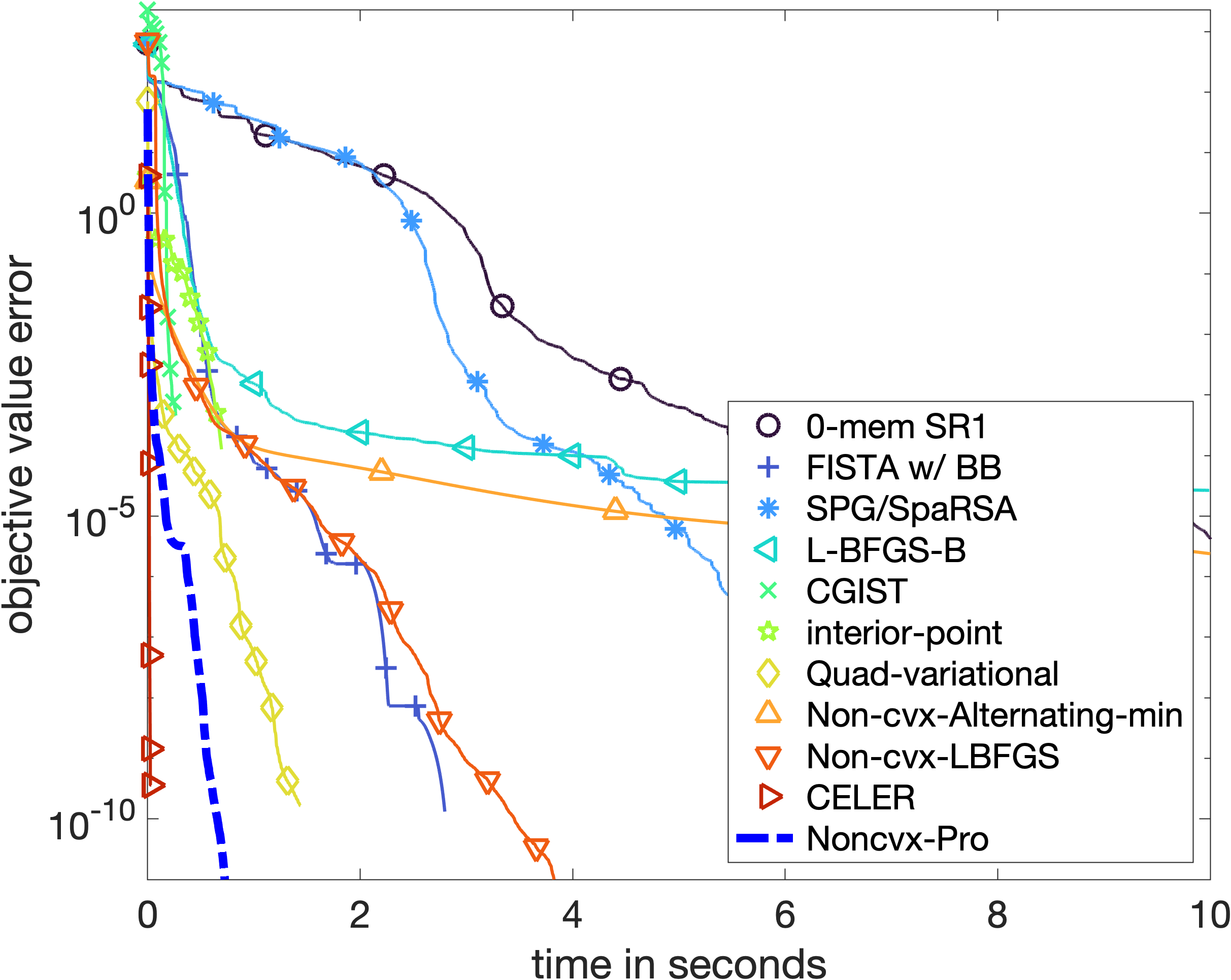
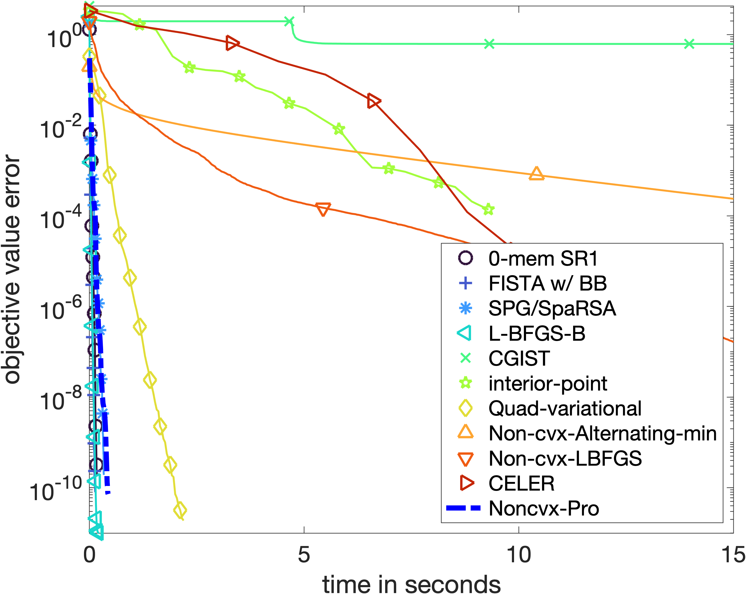
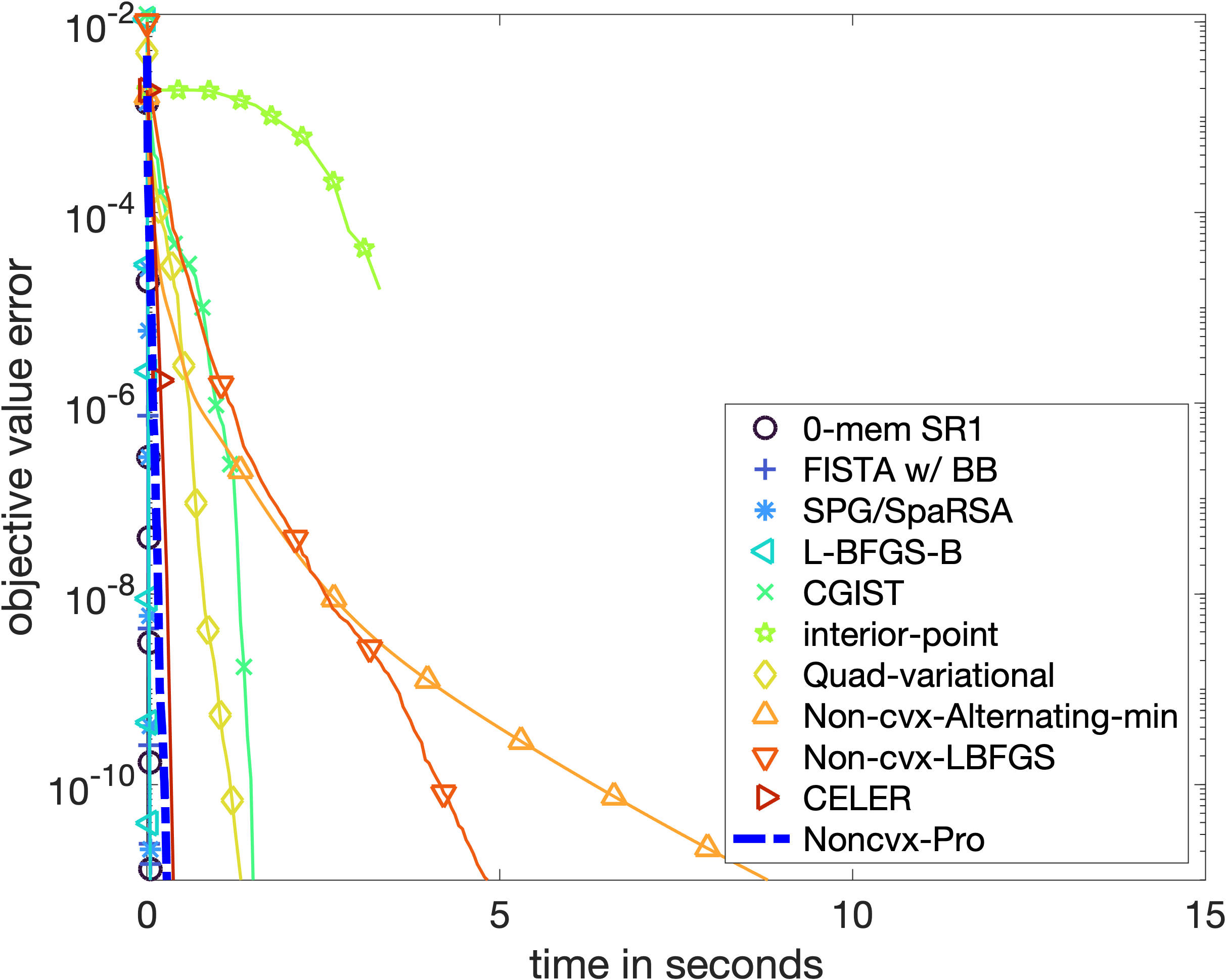
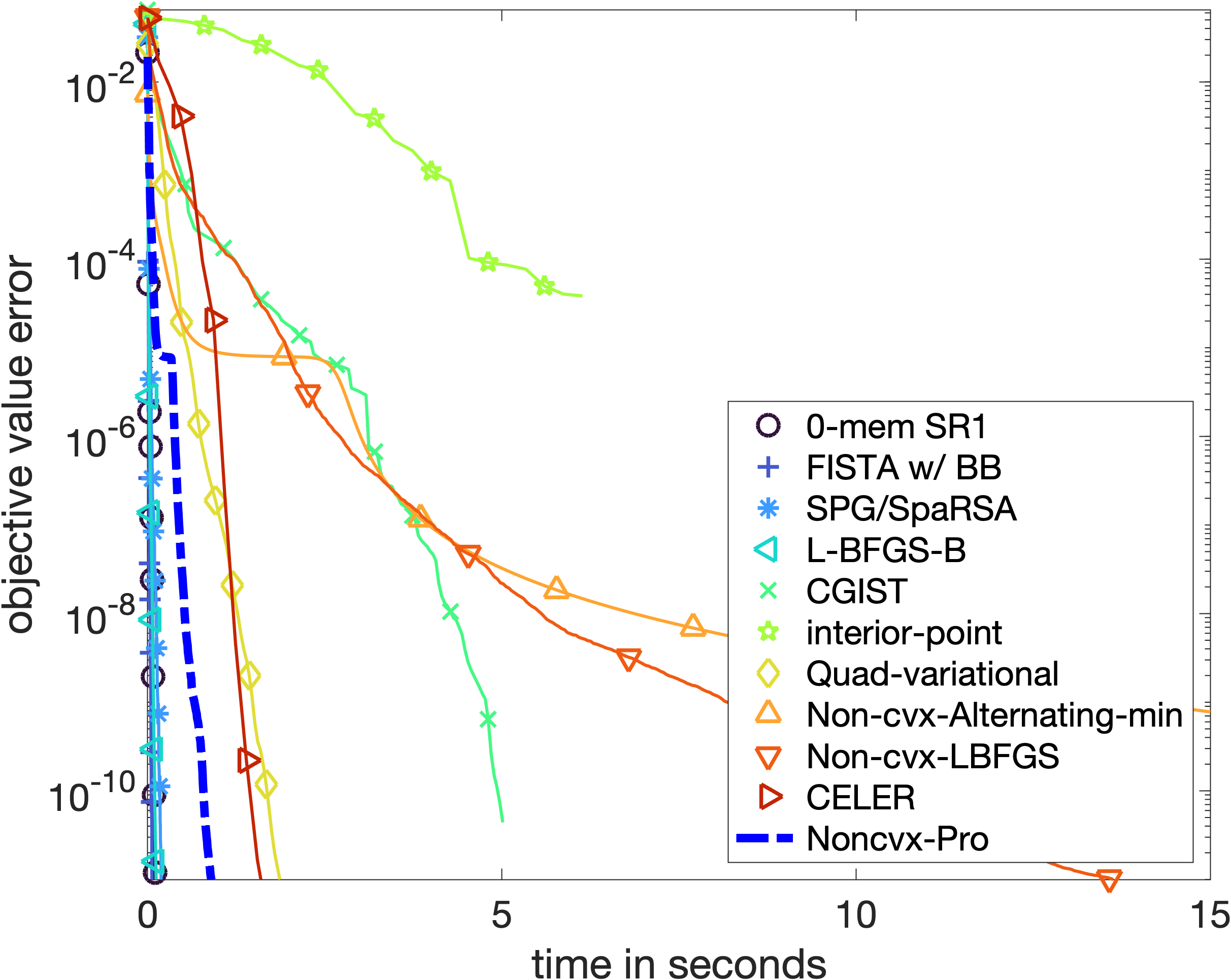
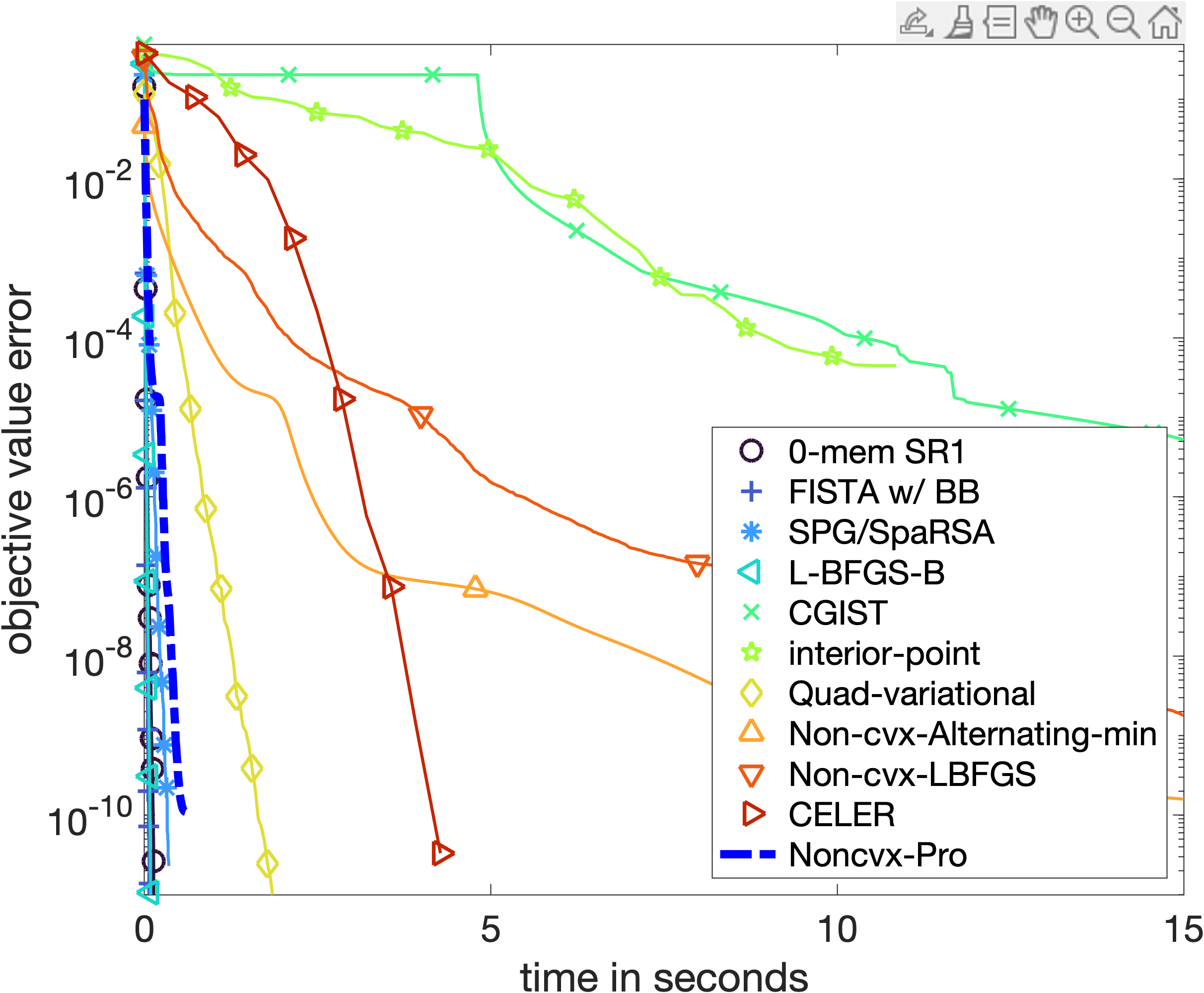
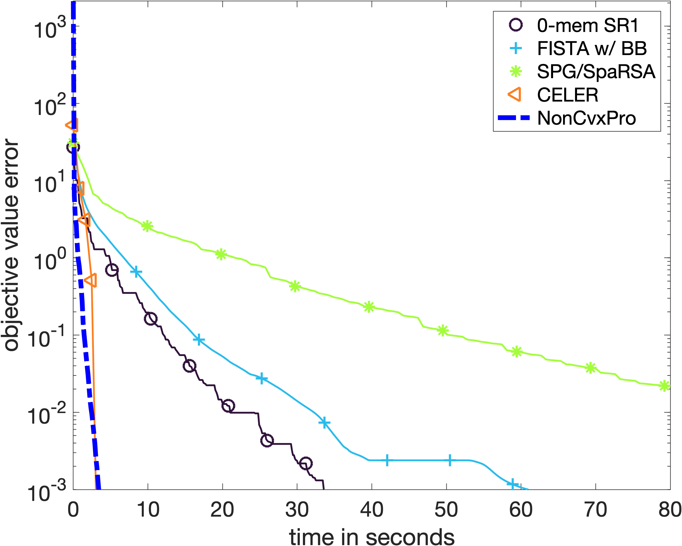
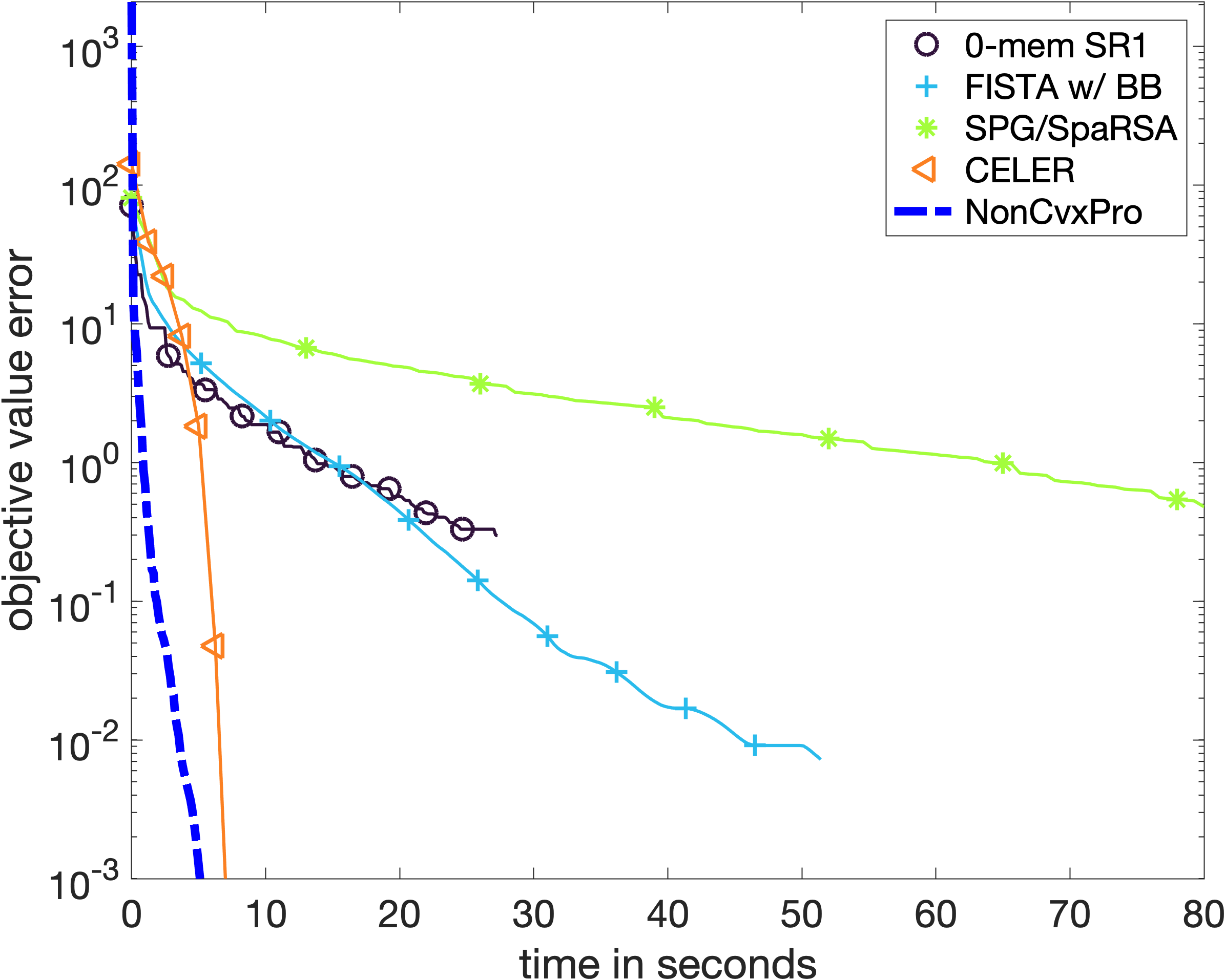
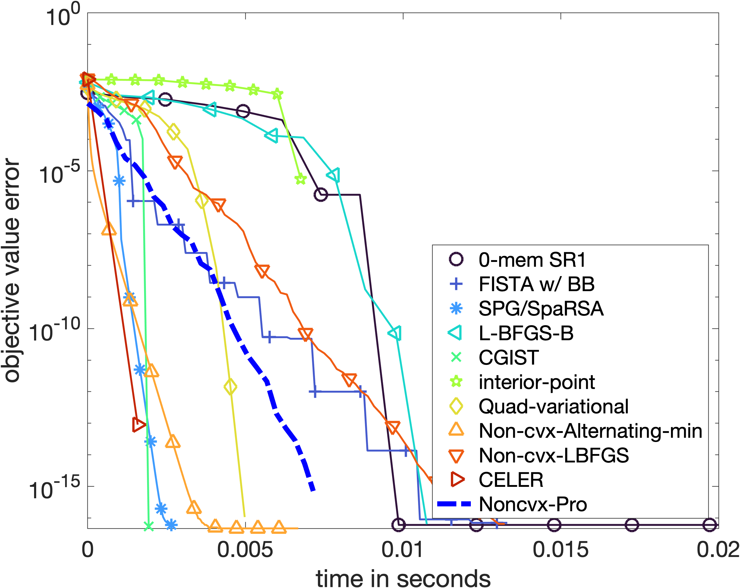
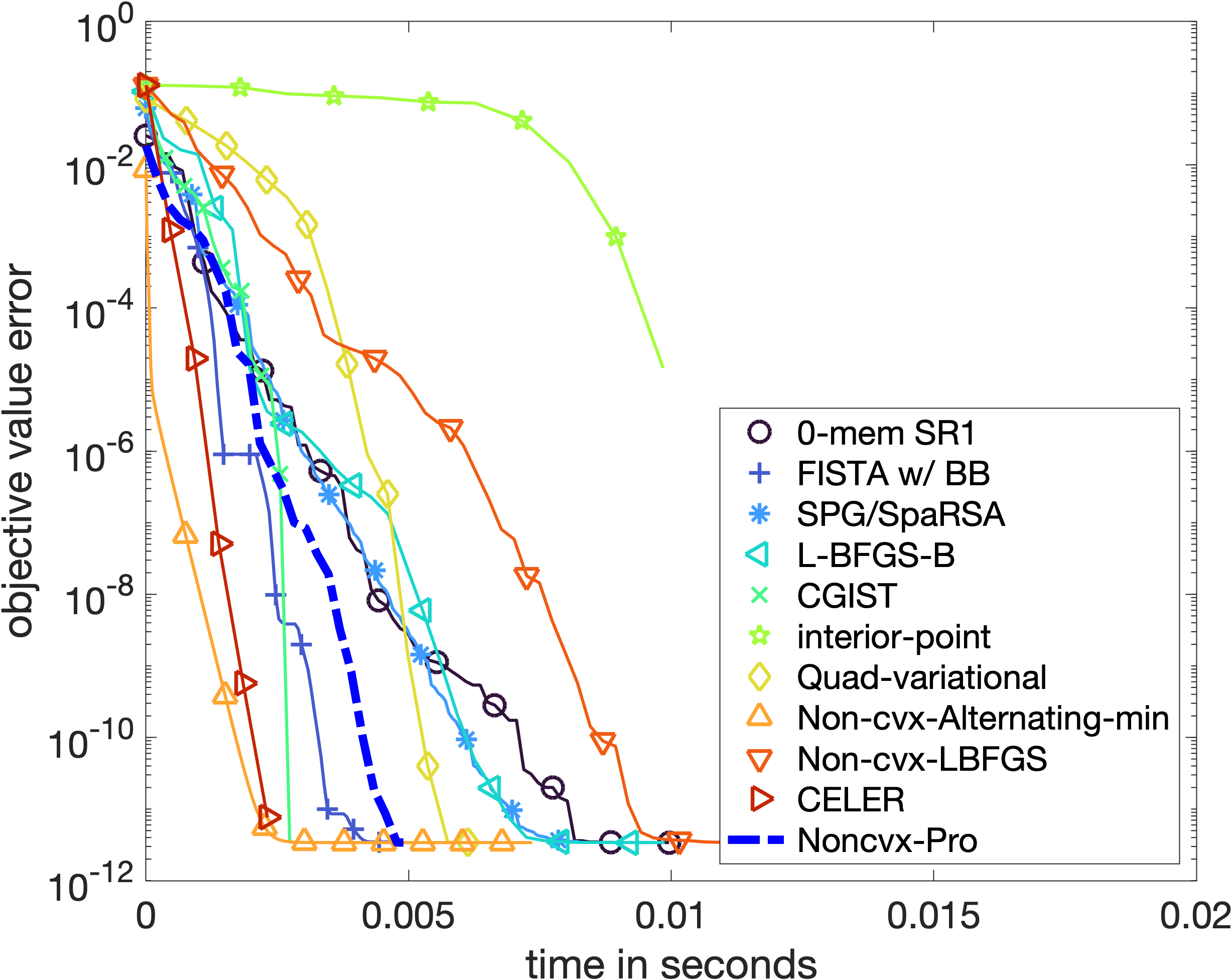
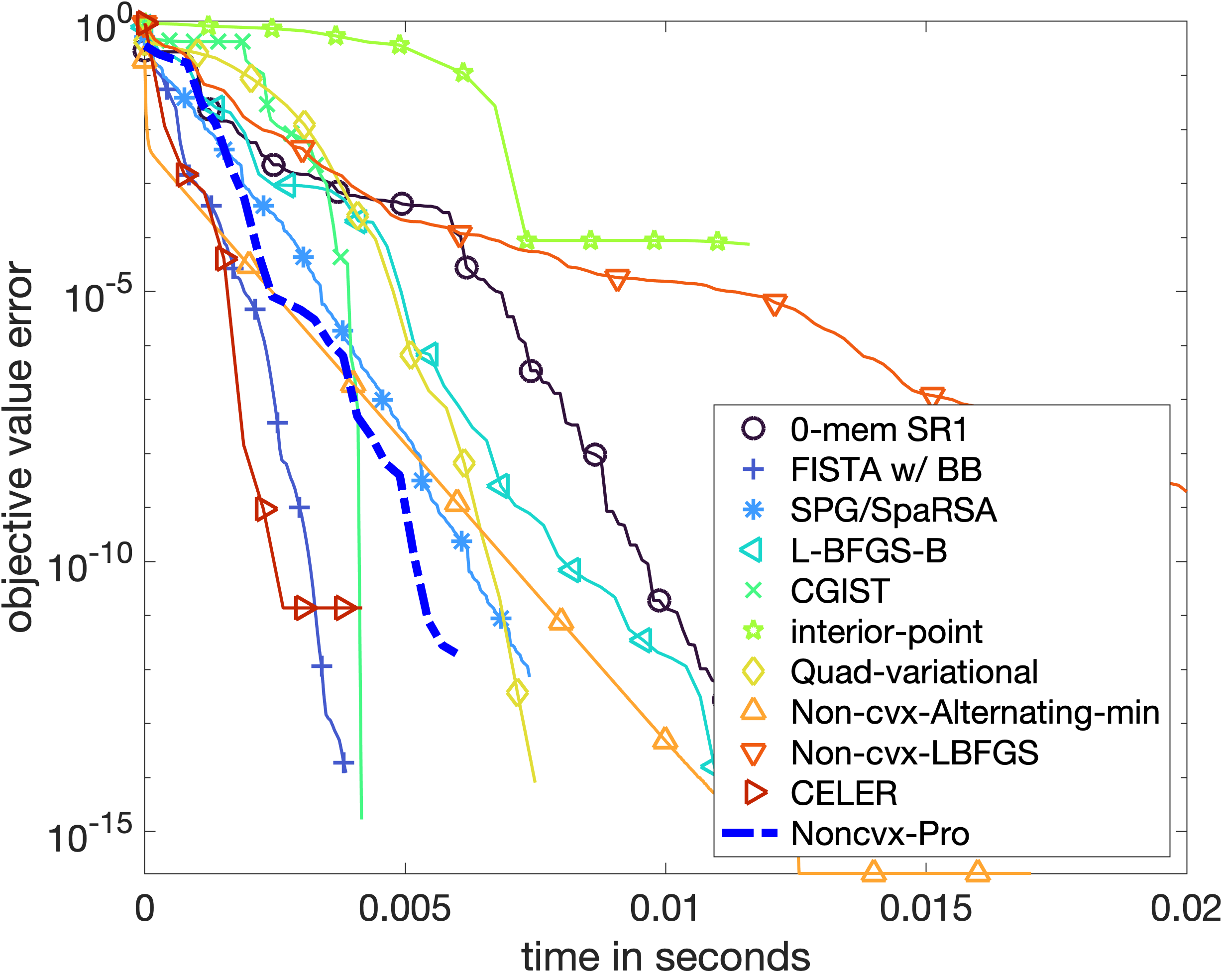
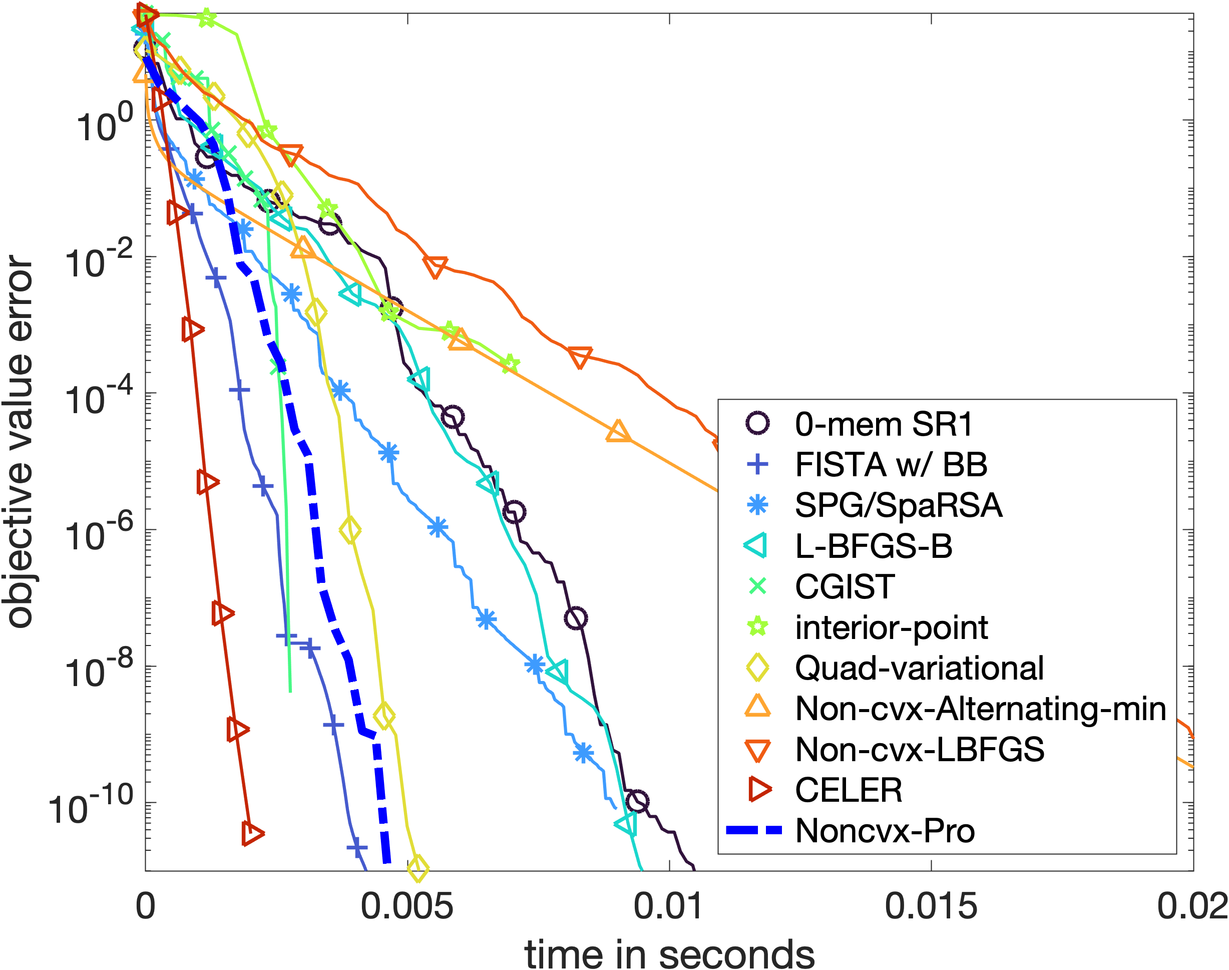
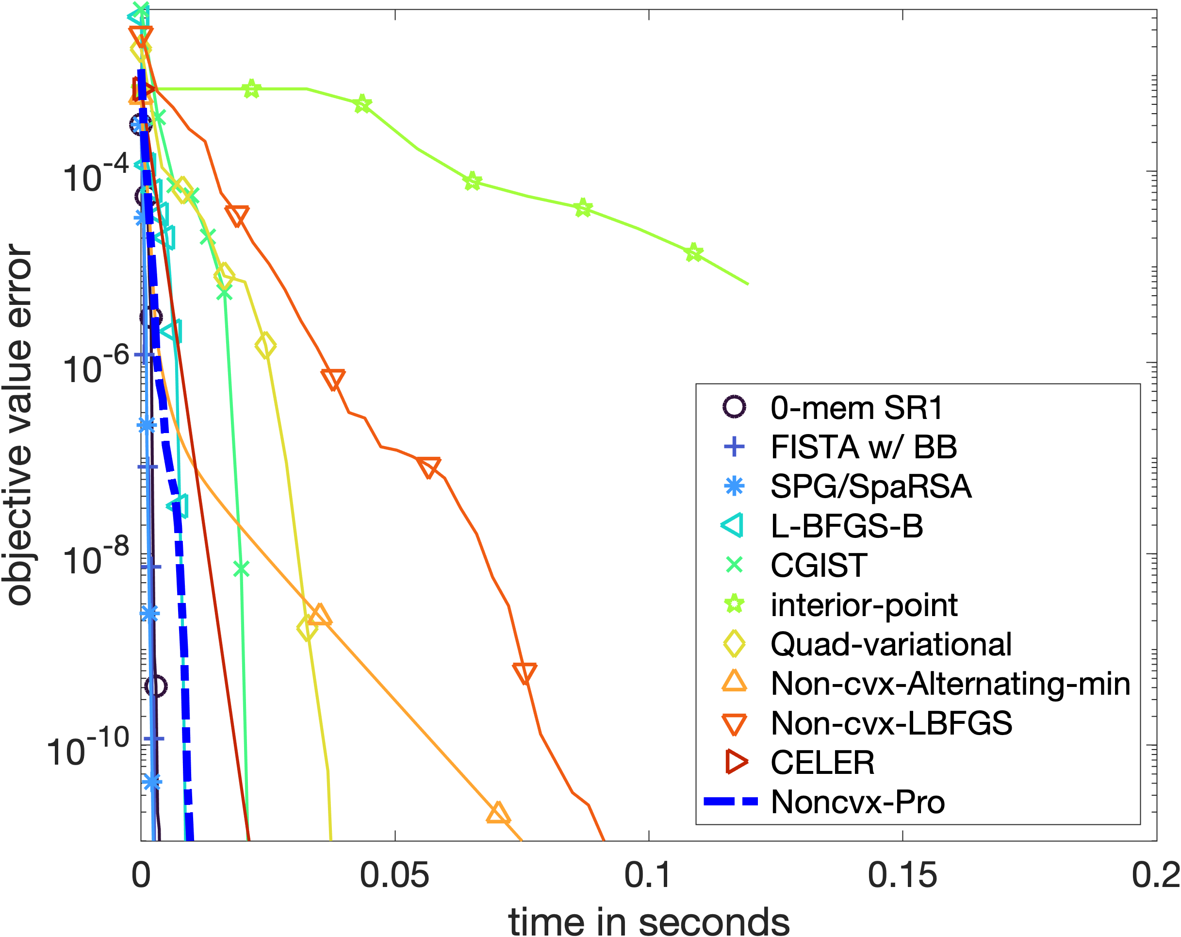
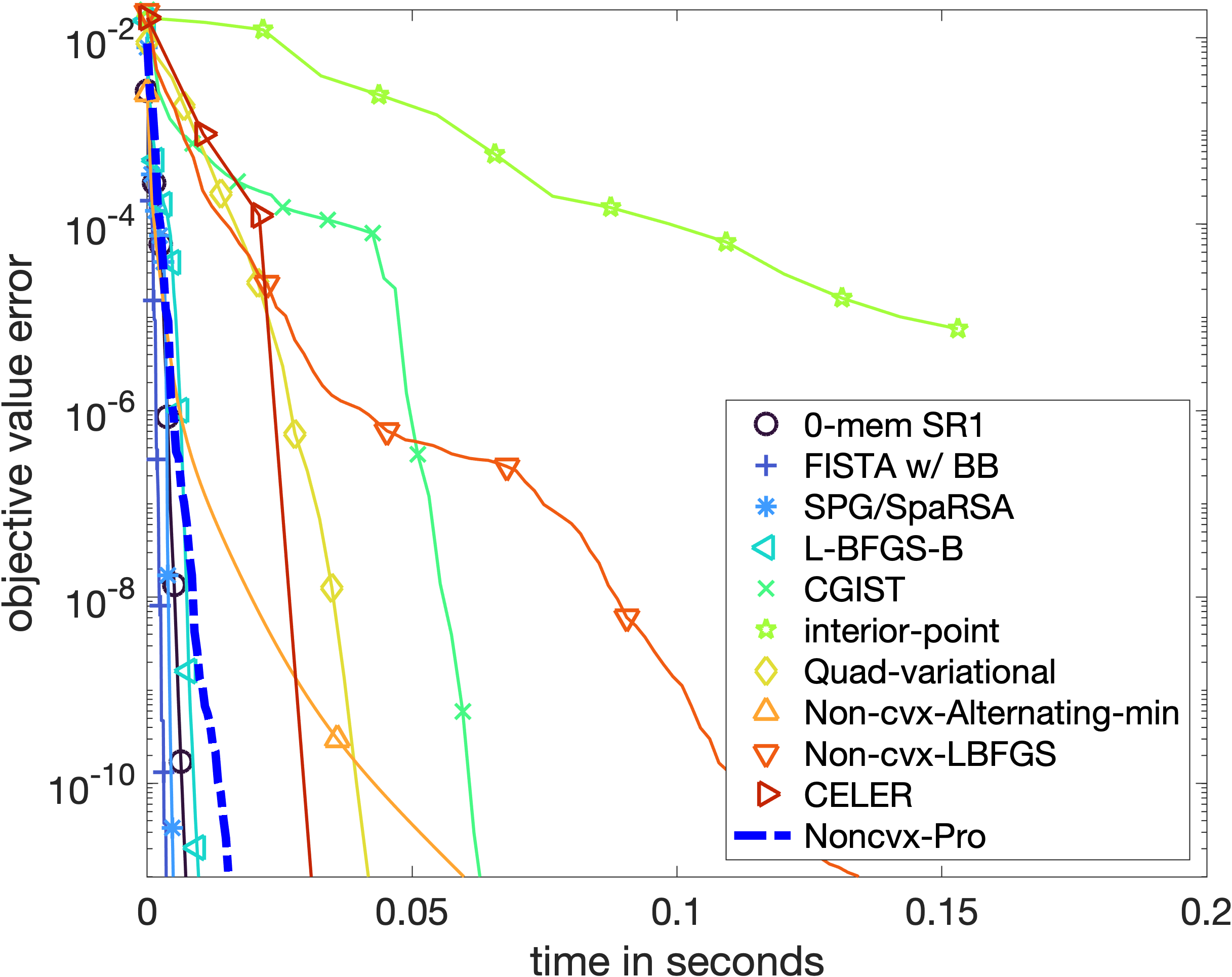
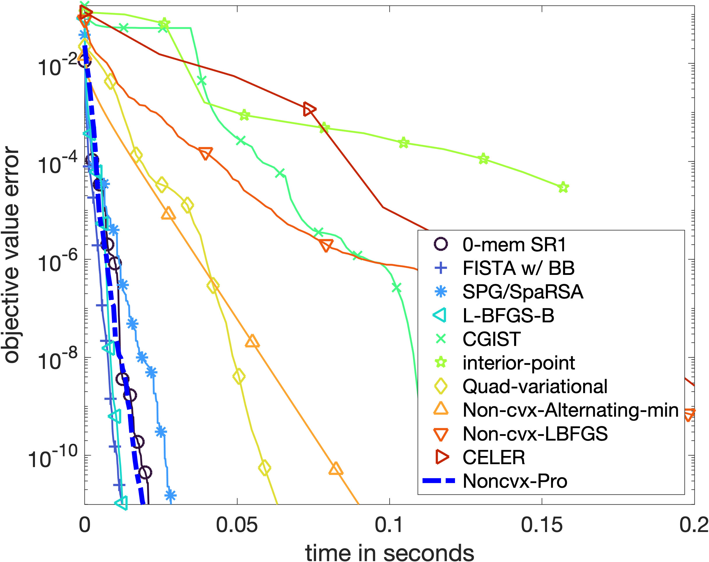
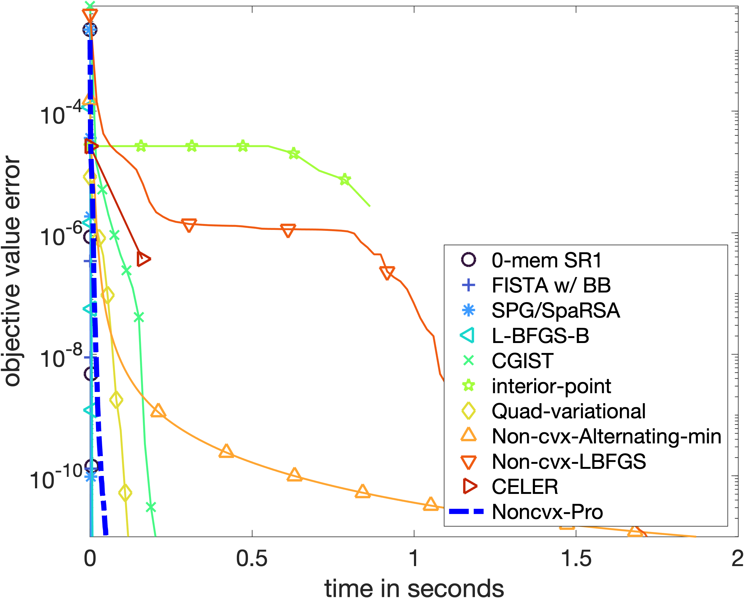
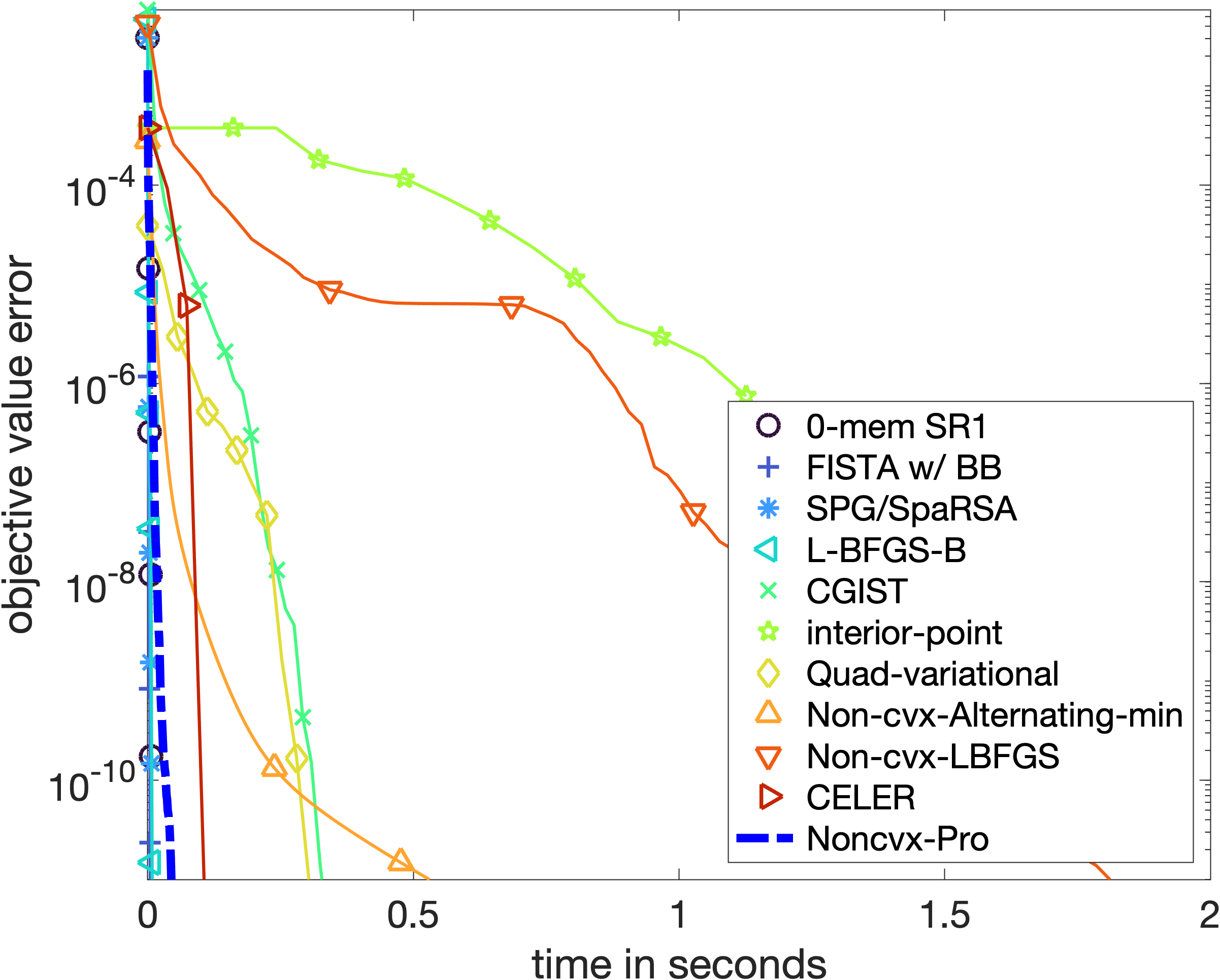
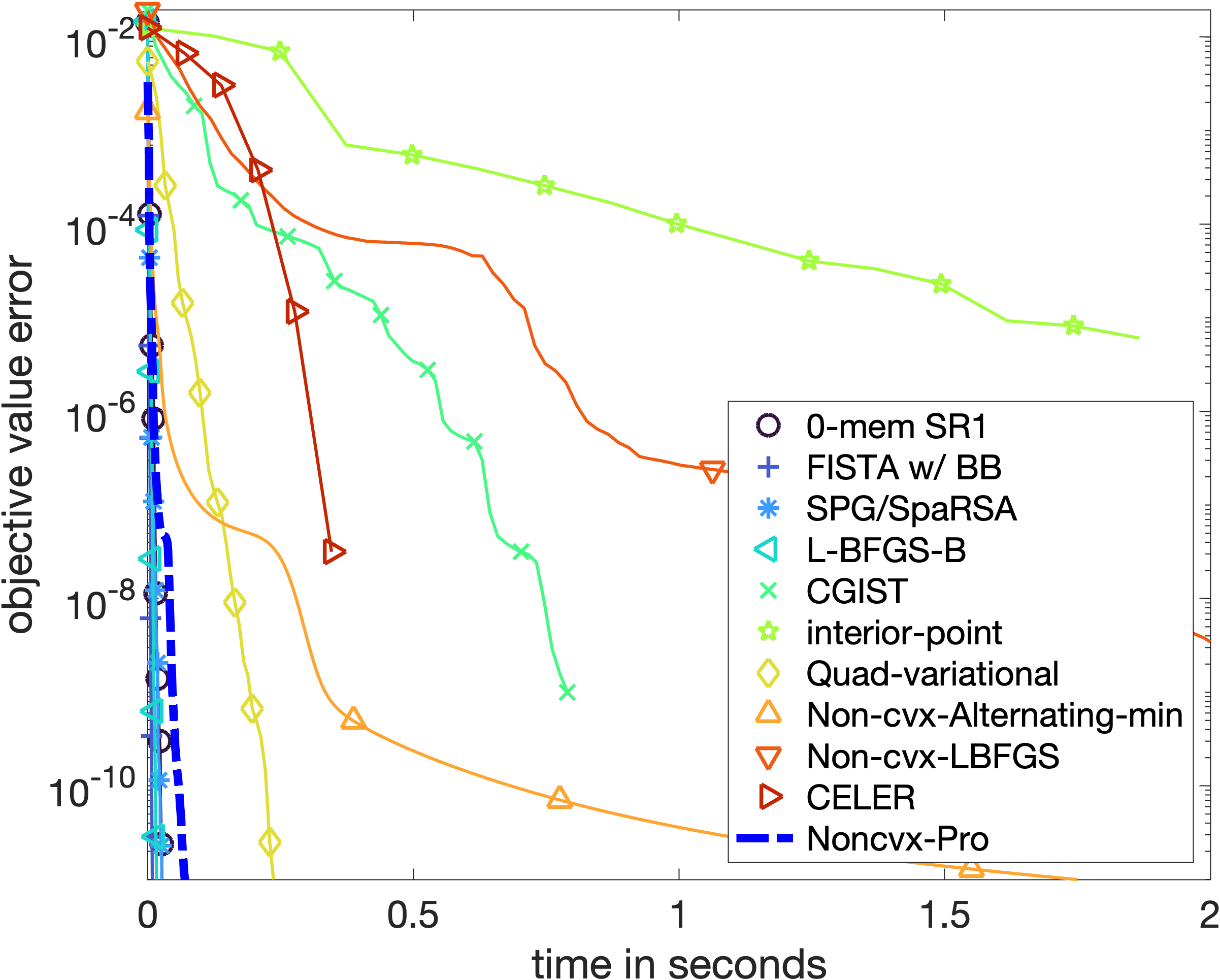
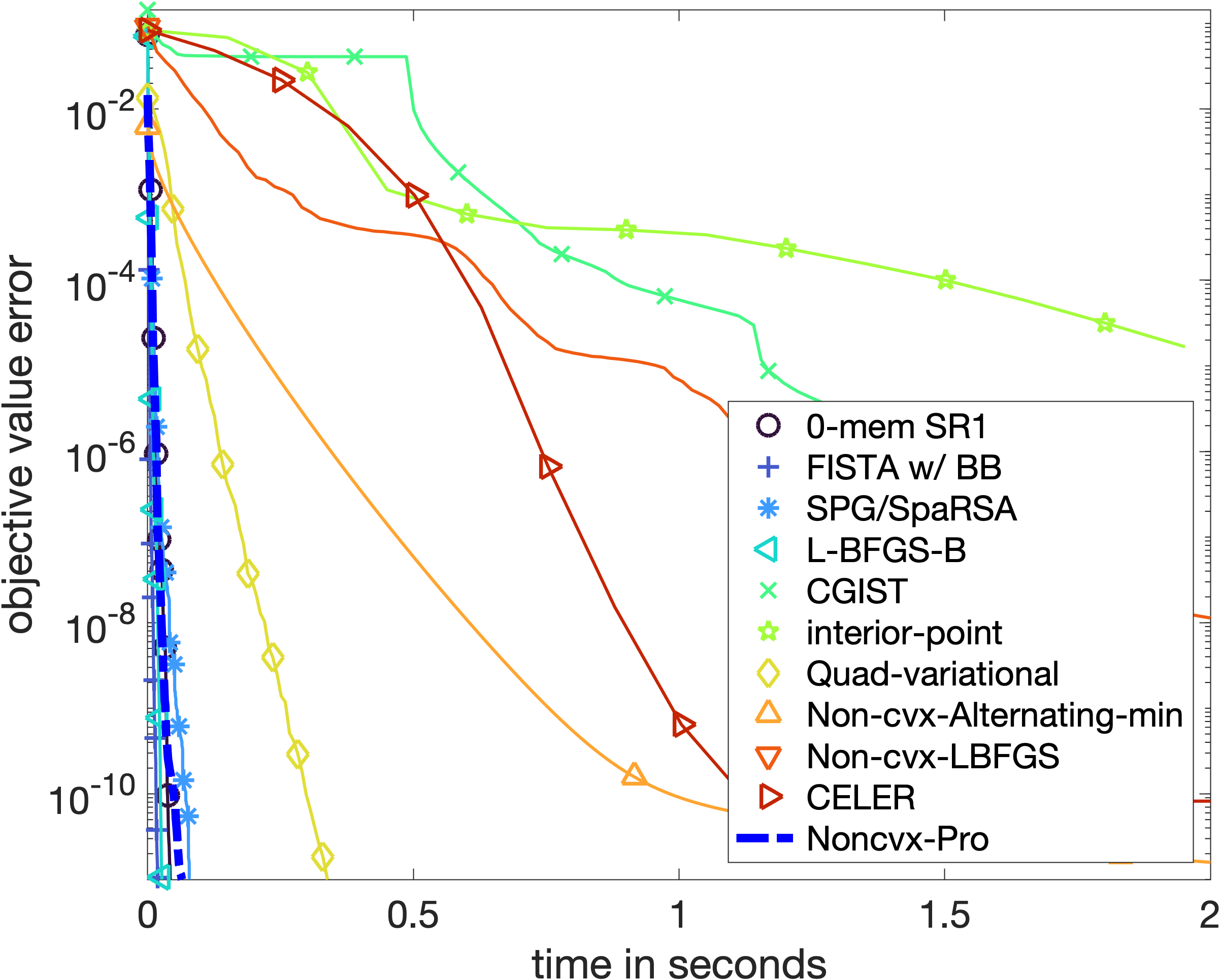
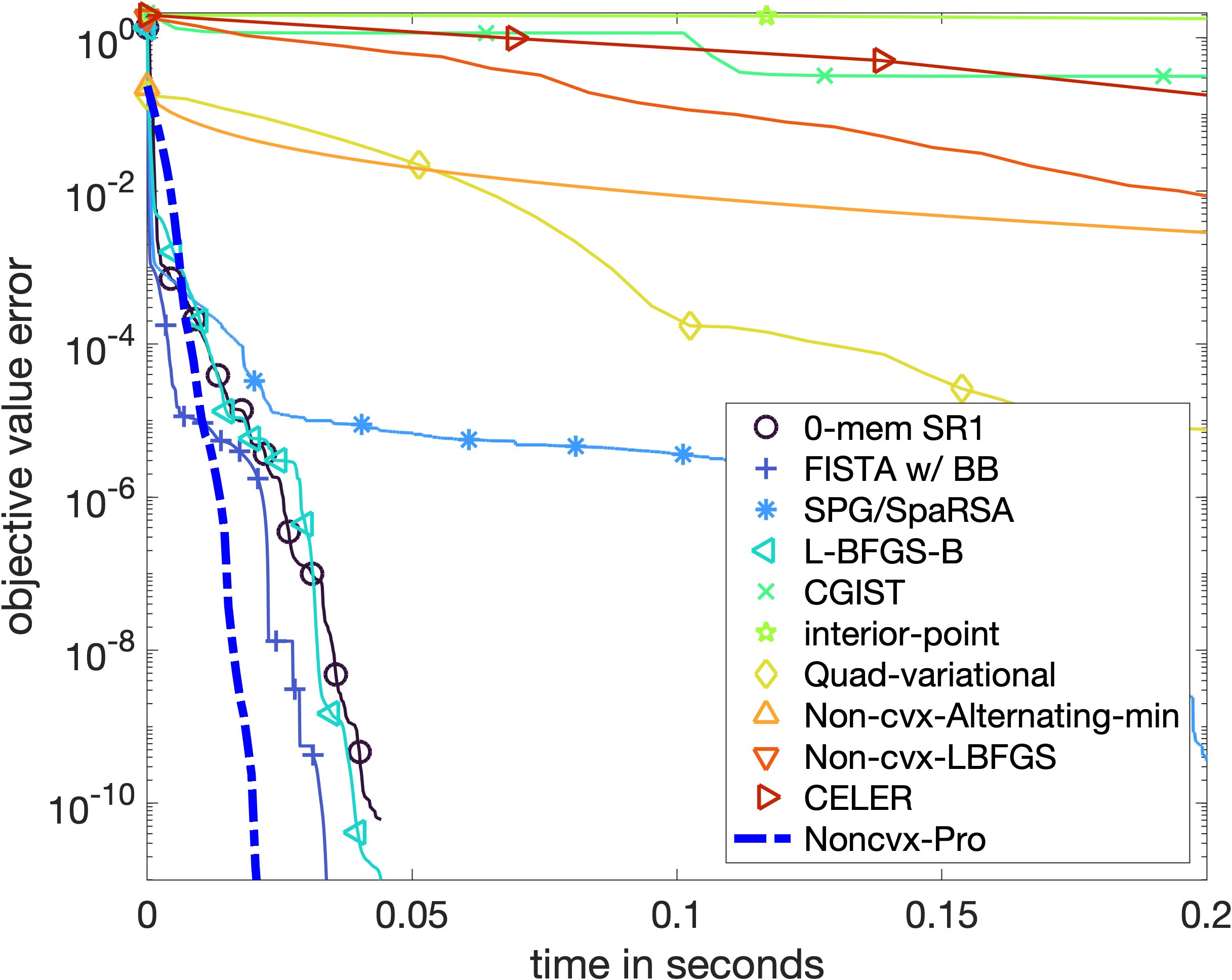
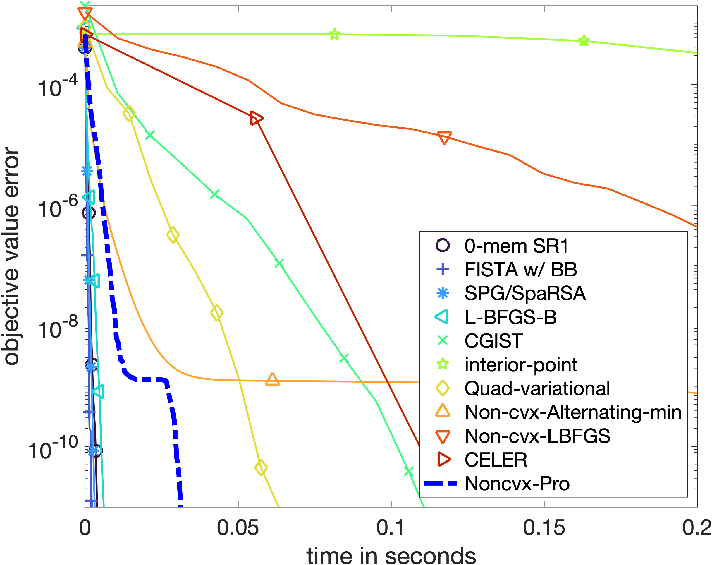
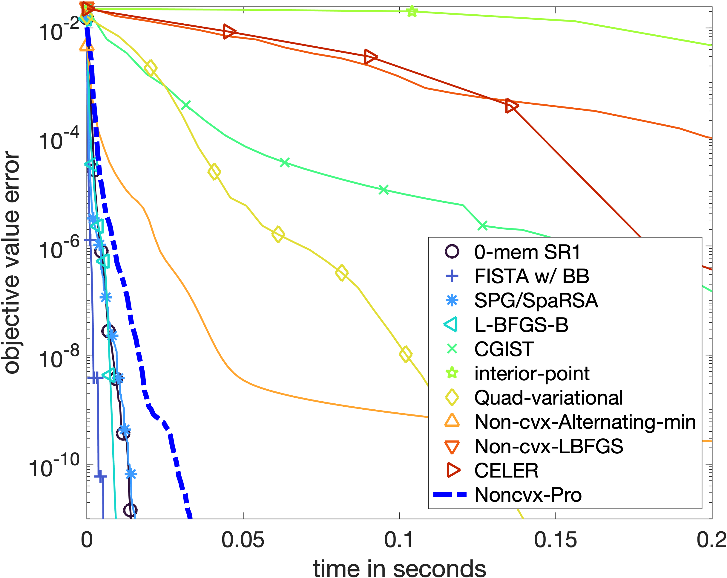
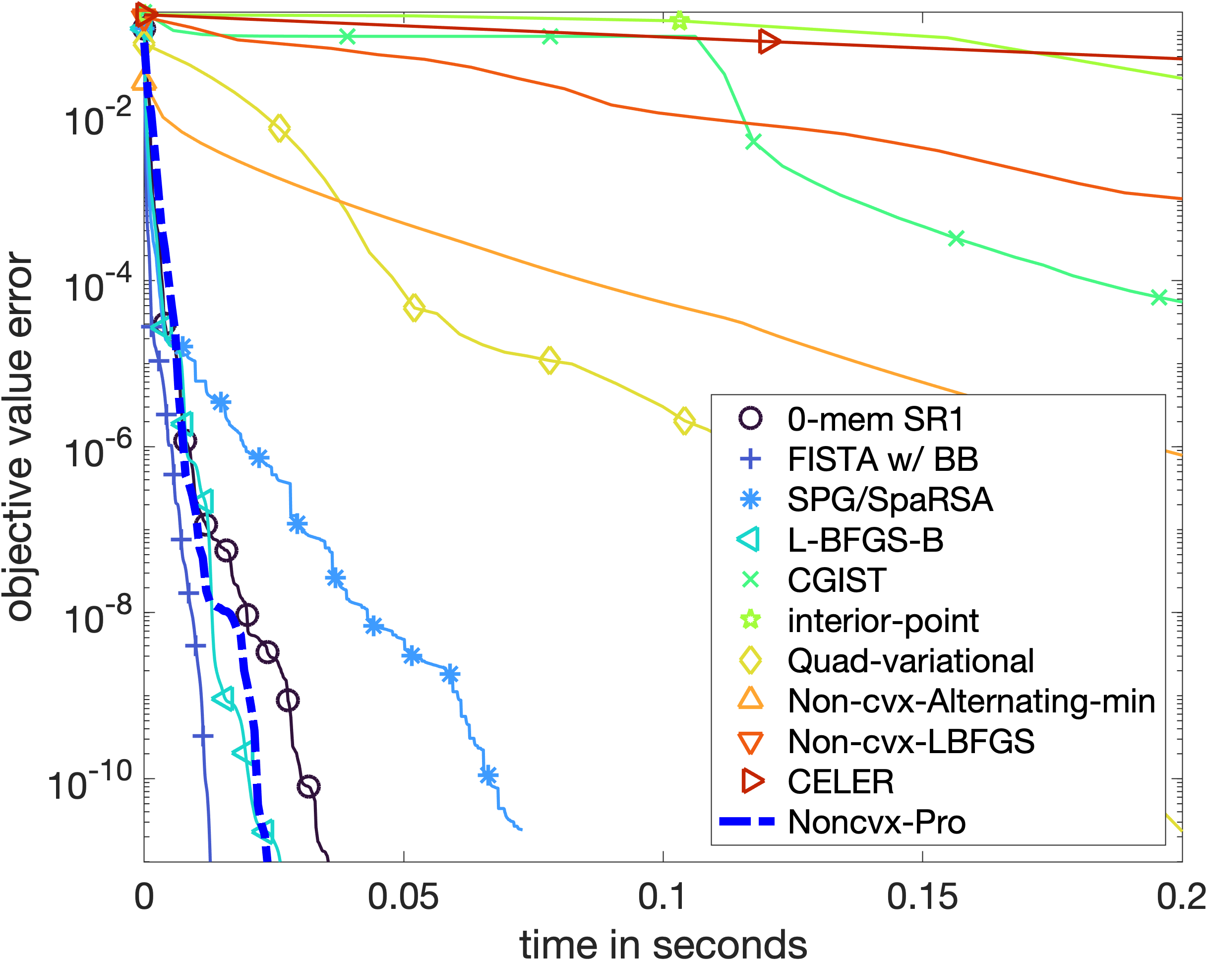
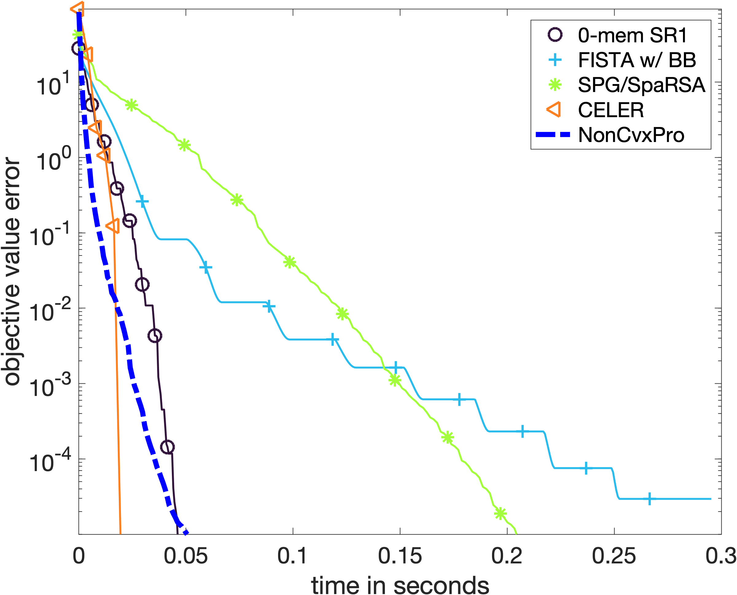
In this section, we use L-BFGS [13] to optimise our bilevel function $f$ and we denote the resulting algorithm “Noncvx-Pro”. Throughout, the inner problem is solved exactly using either a full or a sparse Cholesky solver. One observation from our numerics below is that although Noncvx-Pro is not always the best performing, unlike other solvers, it is robust to a wide range of settings: for example, our solver is mostly unaffected by the choice of $\lambda$ while one can observe in Figures 2 and 3 that this has a large impact on the proximal based methods and coordinate descent. Moreover, Noncvx-Pro is simple to code and rely on existing robust numerical routines (Cholesky/ conjugate gradient + BFGS) which naturally handle sparse/implicit operators, and we thus inherit their nice convergence properties. All numerics are conducted on 2.4 GHz Quad-Core Intel Core i5 processor with 16GB RAM. The code to reproduce the results of this article is available online.

4.1 Lasso

We first consider the Lasso problem where $R(\beta)=\sum_{i=1}^{n}|\beta_{i}|$.

Datasets.

We tested on 8 datasets from the Libsvm repository. These datasets are mean subtracted and normalised by $m$.

Solvers.

We compare against the following 10 methods:

1. 0-mem SR1: a proximal quasi newton method [7].

2. FISTA w/ BB: FISTA with Barzilai–Borwein stepsize [5] and restarts [45].

3. SPG/SpaRSA: spectral projected gradient [58].

4. CGIST: an active set method with conjugate gradient iterative shrinkage/thresholding [27].

5. Interior point method: from [35].

6. CELER: a coordinate descent method with support pruning [39].

7. Non-cvx-Alternating-min: alternating minimisation of $u$ and $v$ in $G$ from (3)  [32].

8. Non-cvx-LBFGS: Apply L-BFGS to minimise the function $(u,v)\mapsto G(u,v)$ in (3).

9. L-BFGS-B [13]: apply L-BFGS-B under positivity constraints to $\min_{u,v\in\mathbb{R}^{n}_{+}}\sum_{i}u_{i}+\sum_{i}v_{i}+\frac{1}{2\lambda}|\!|X(u-v)-y|\!|_{2}^{2}$. This is the standard approach for applying L-BFGS to $\ell_{1}$ minimisation and corresponds to splitting $\beta$ into its positive and negative parts.

10. Quad-variational: Based on our idea of Noncvx-Pro, another natural (and to our knowledge novel) approach is to apply L-BFGS-B to the bilevel formulation of (1) without nonconvex reparametrization. Indeed, by applying (1) and using convex duality, the Lasso can solved by minimizing $g(\eta)\triangleq\max_{\alpha\in\mathbb{R}^{m}}\frac{1}{2}\sum_{i}\eta_{i}-\frac{\lambda}{2}|\!|\alpha|\!|^{2}-\frac{1}{2}\sum_{i}\eta_{i}|\langle x_{i},\,\alpha\rangle|^{2}+\langle\alpha,\,y\rangle$. The gradient of $g$ is $g(\eta)=\frac{\lambda}{2}-\frac{1}{\lambda}|X^{\top}\alpha|^{2}$ where $|\cdot|^{2}$ is in a pointwise sense and $\alpha$ maximises the inner problem, and we apply L-BFGS-B with positivity constraints to minimise $g$.

Experiments.

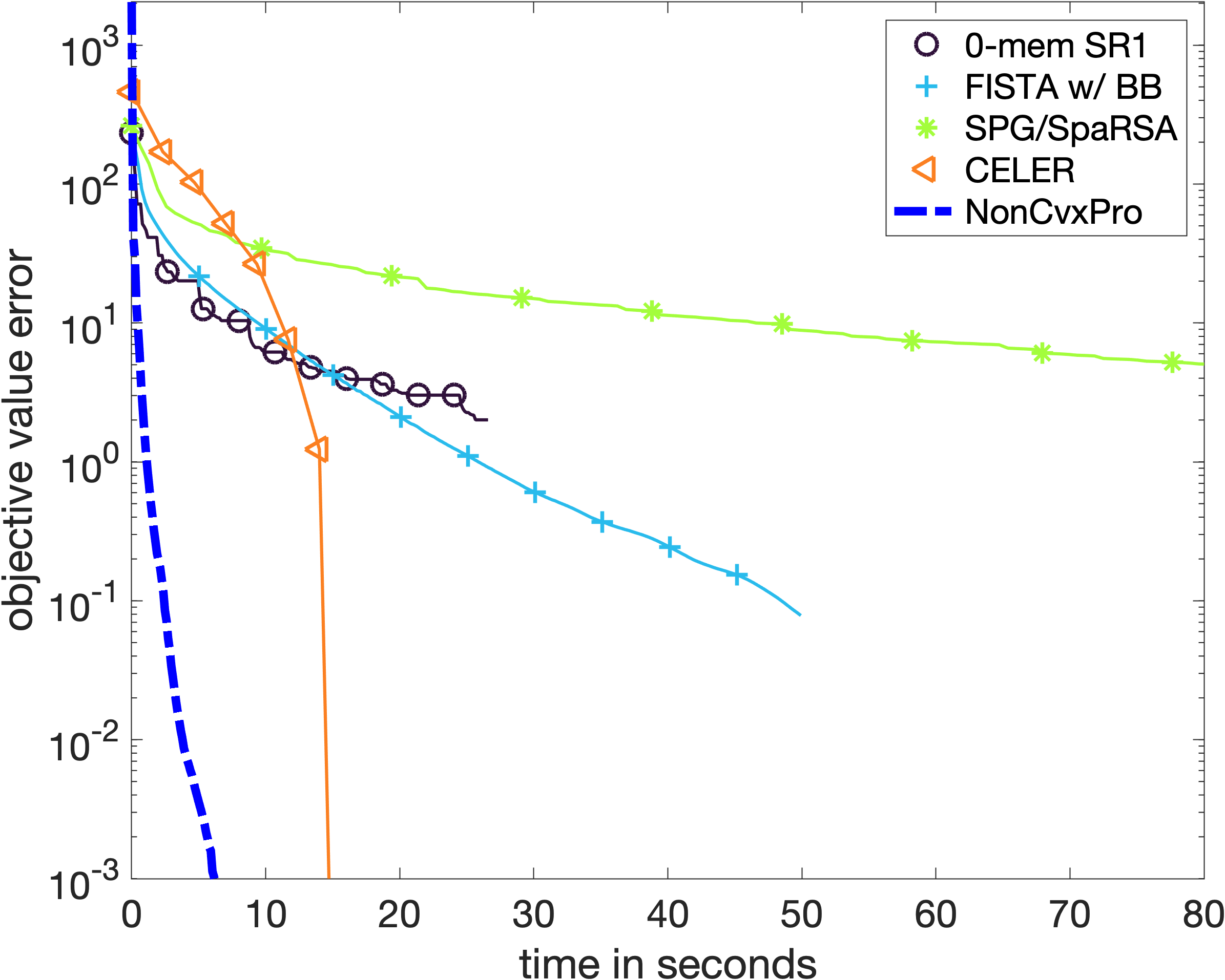
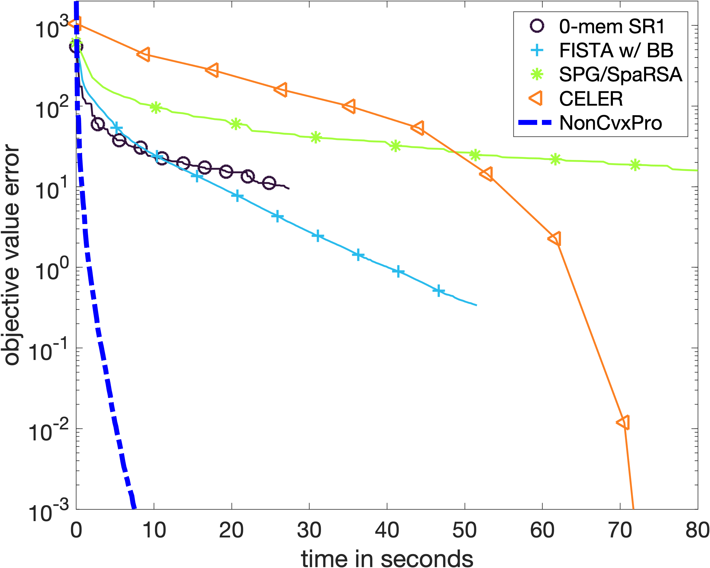
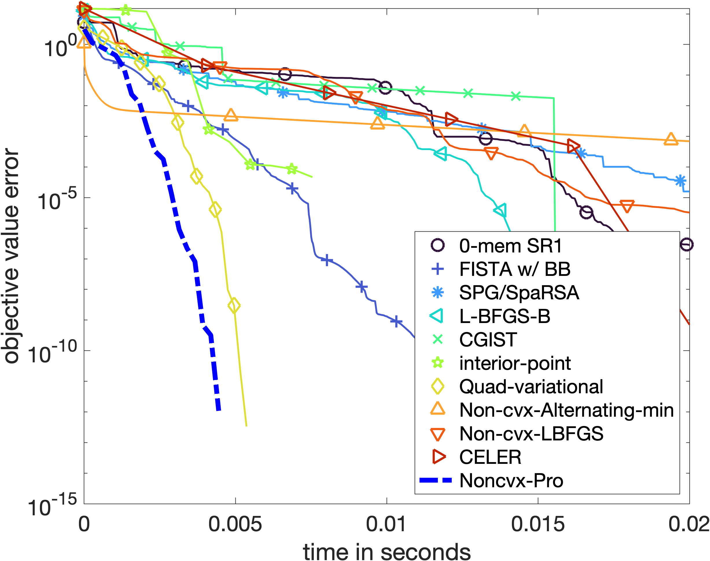
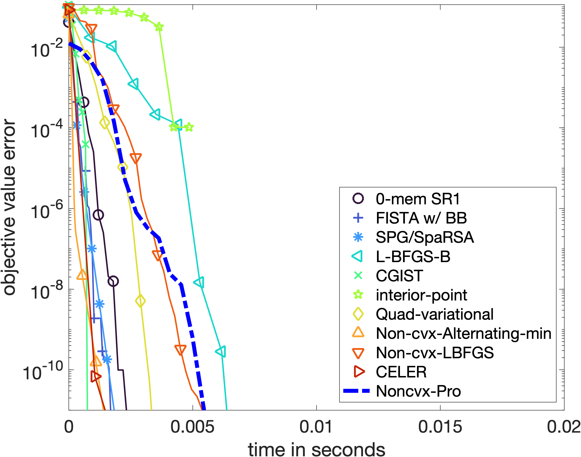
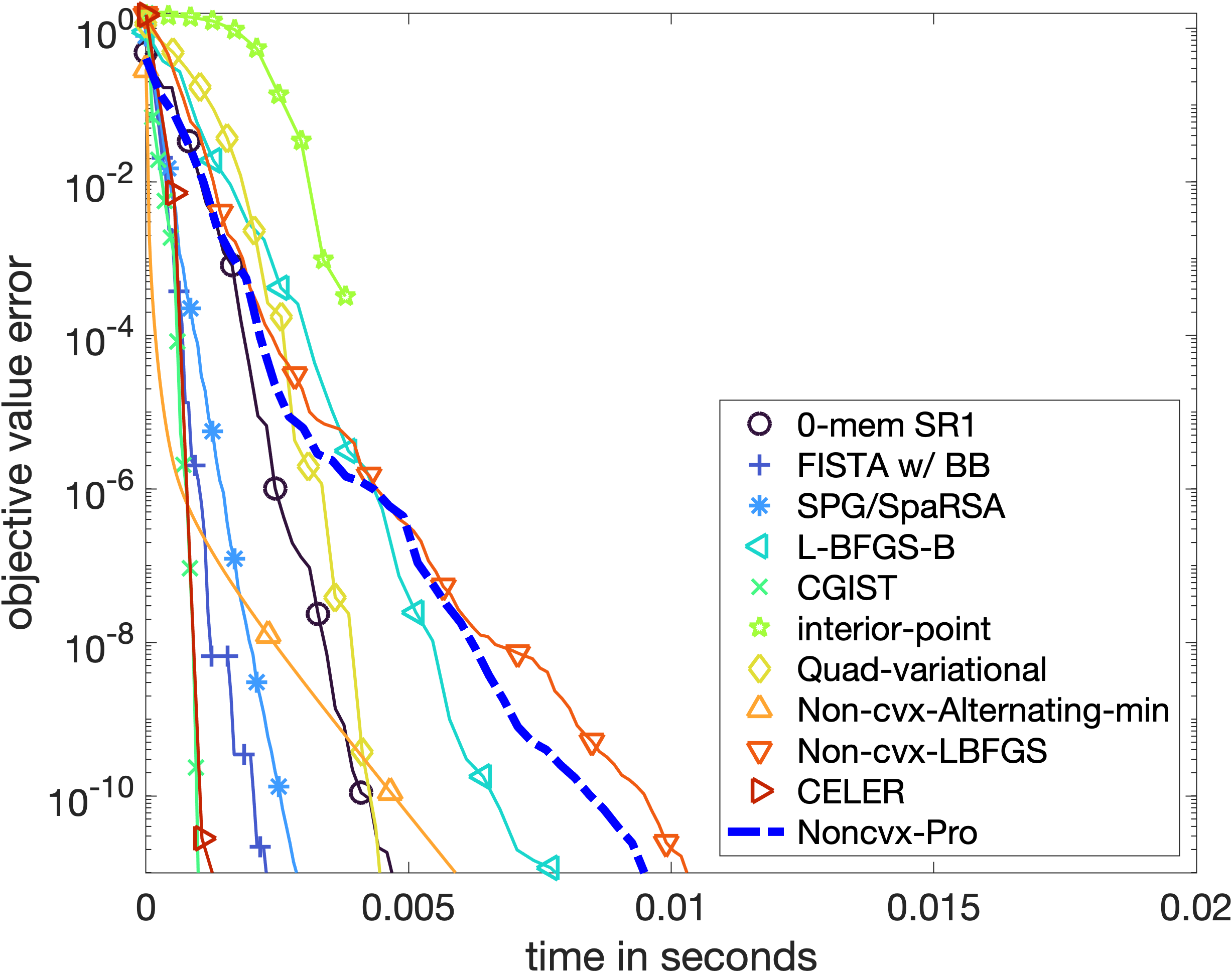
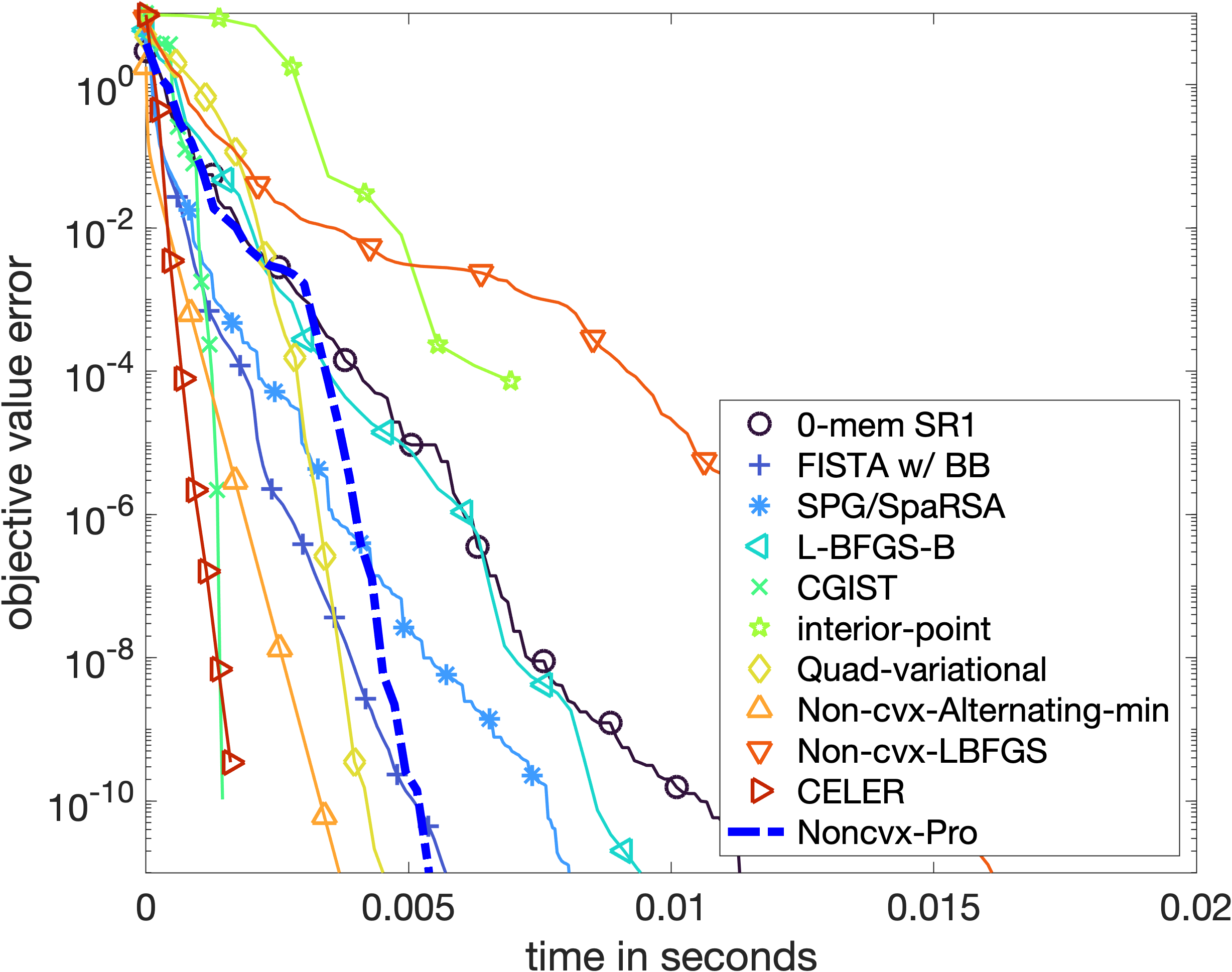
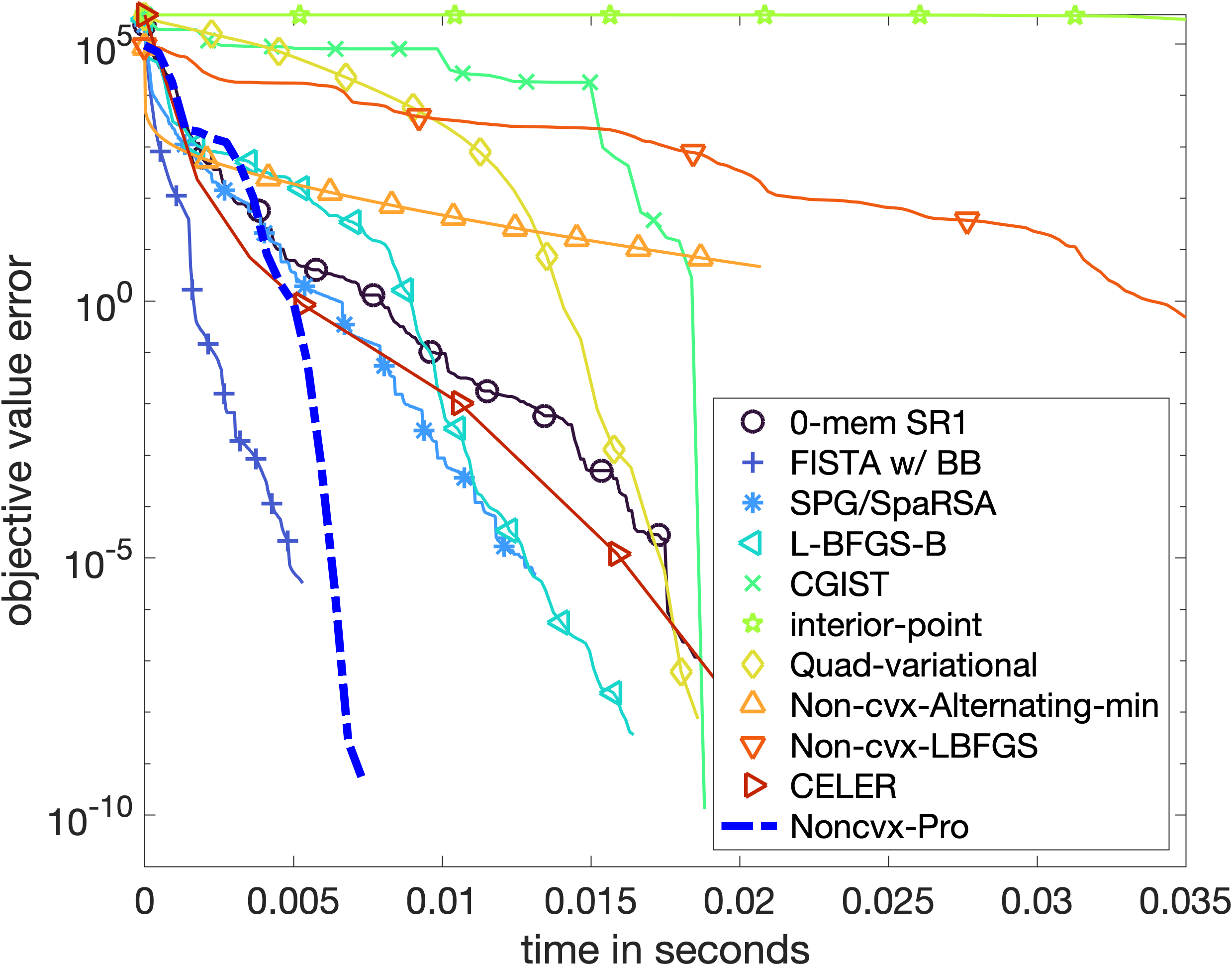
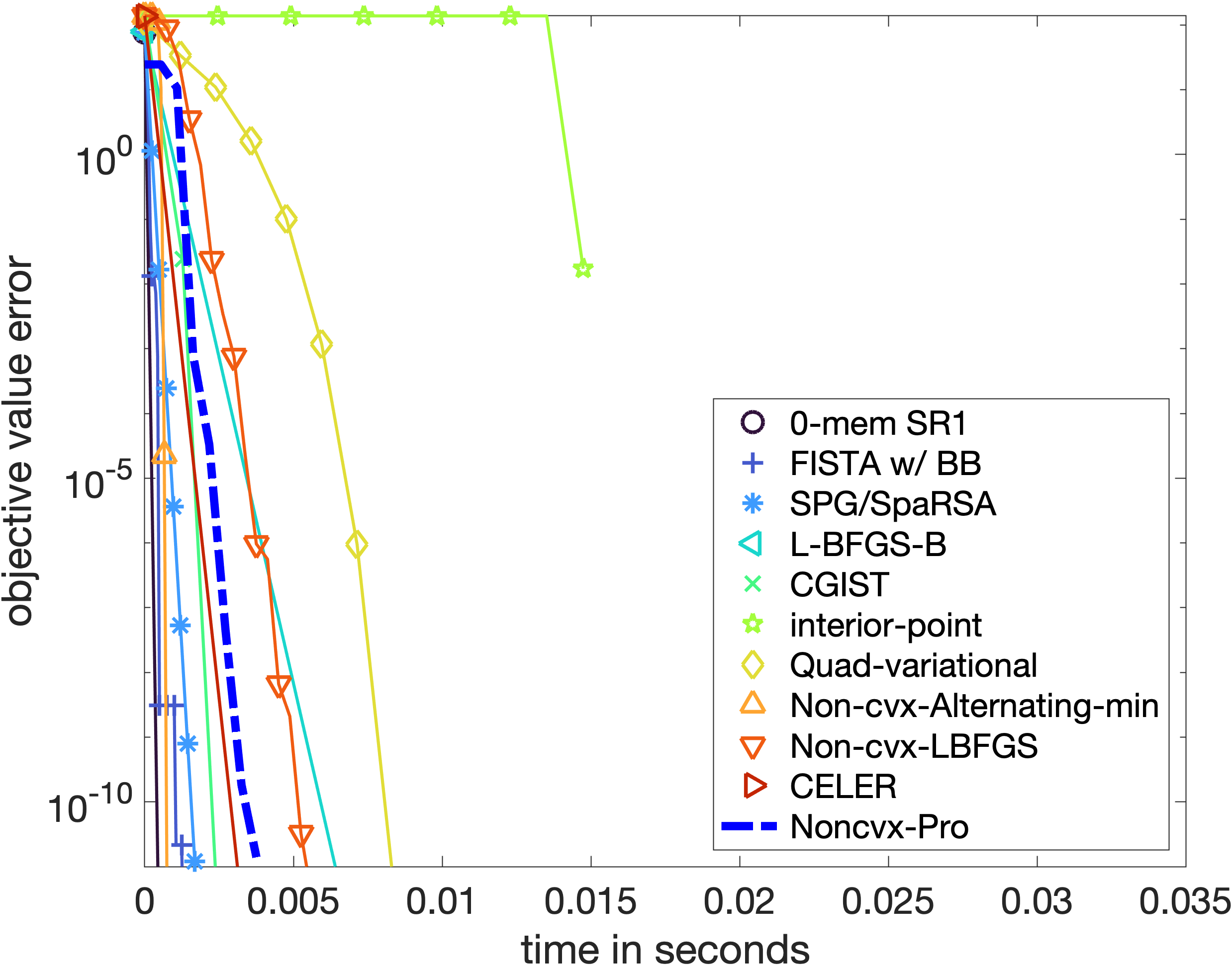
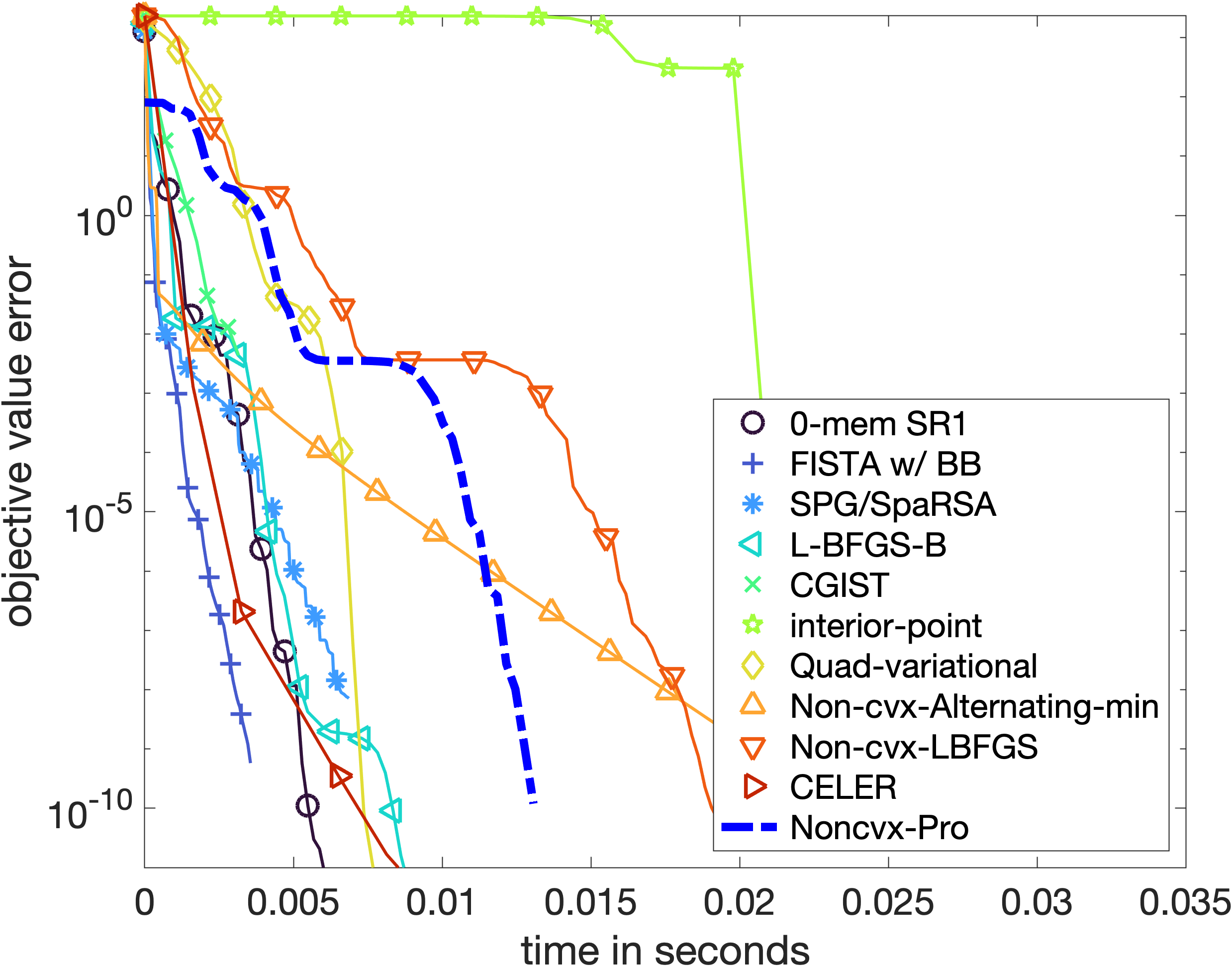
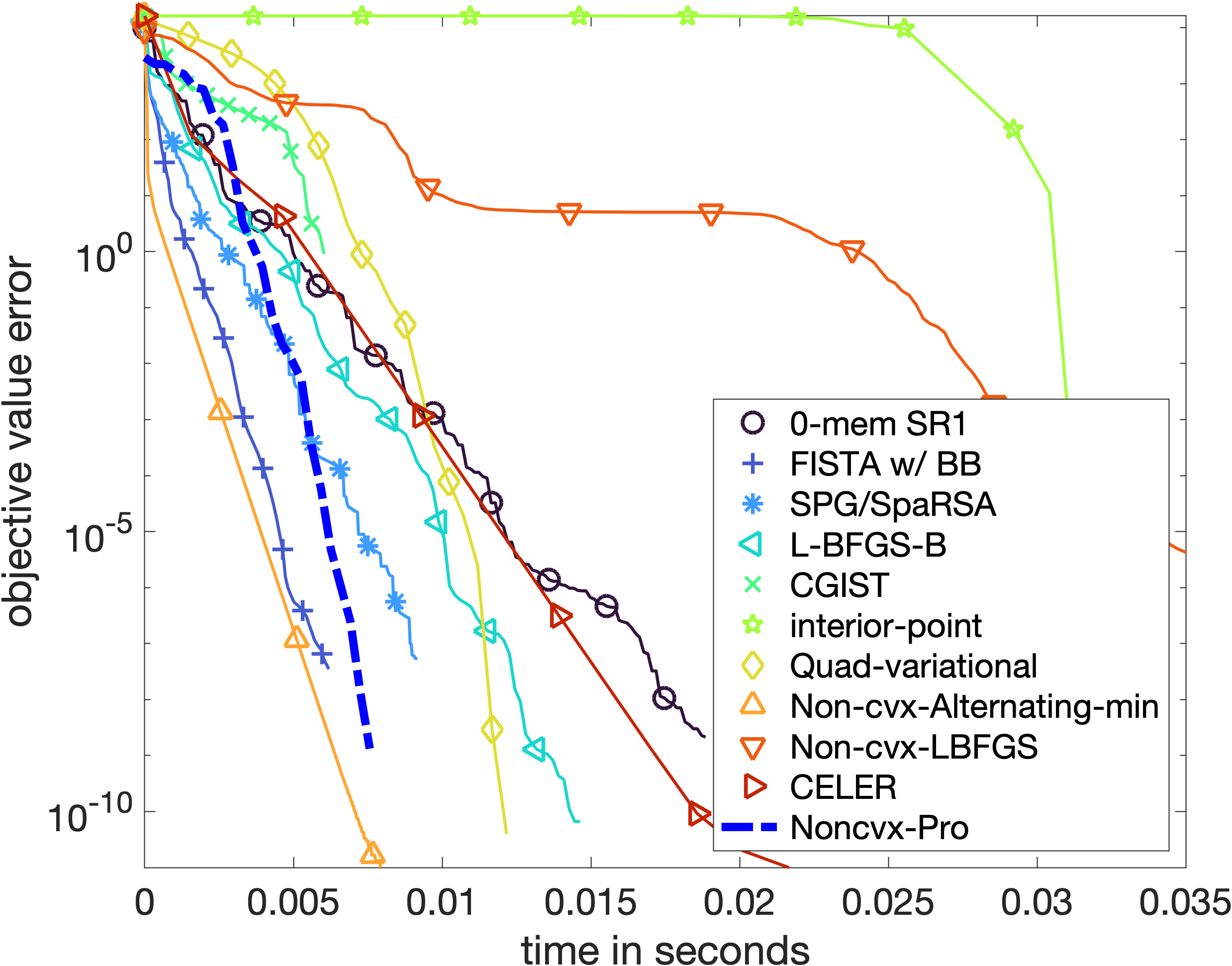
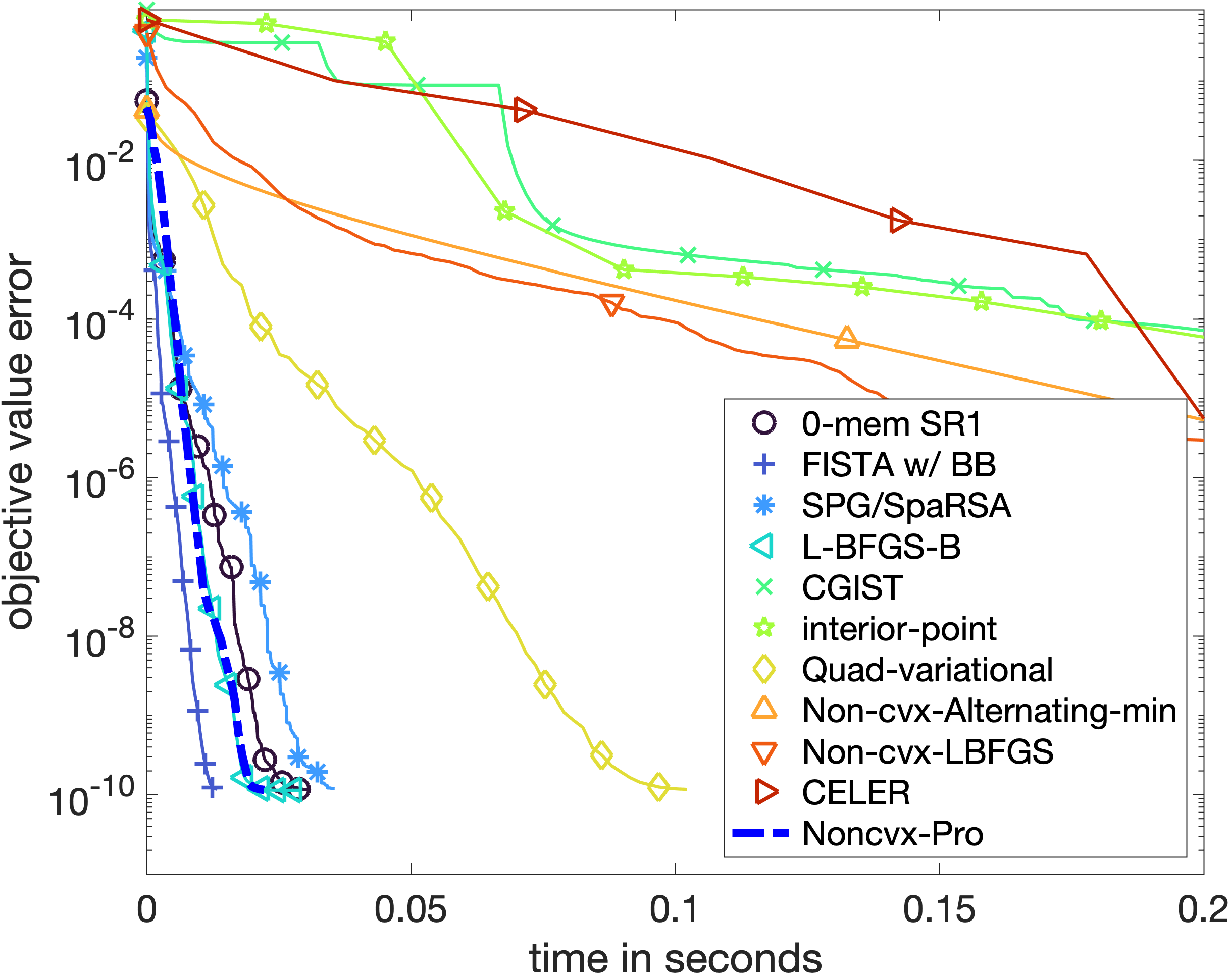
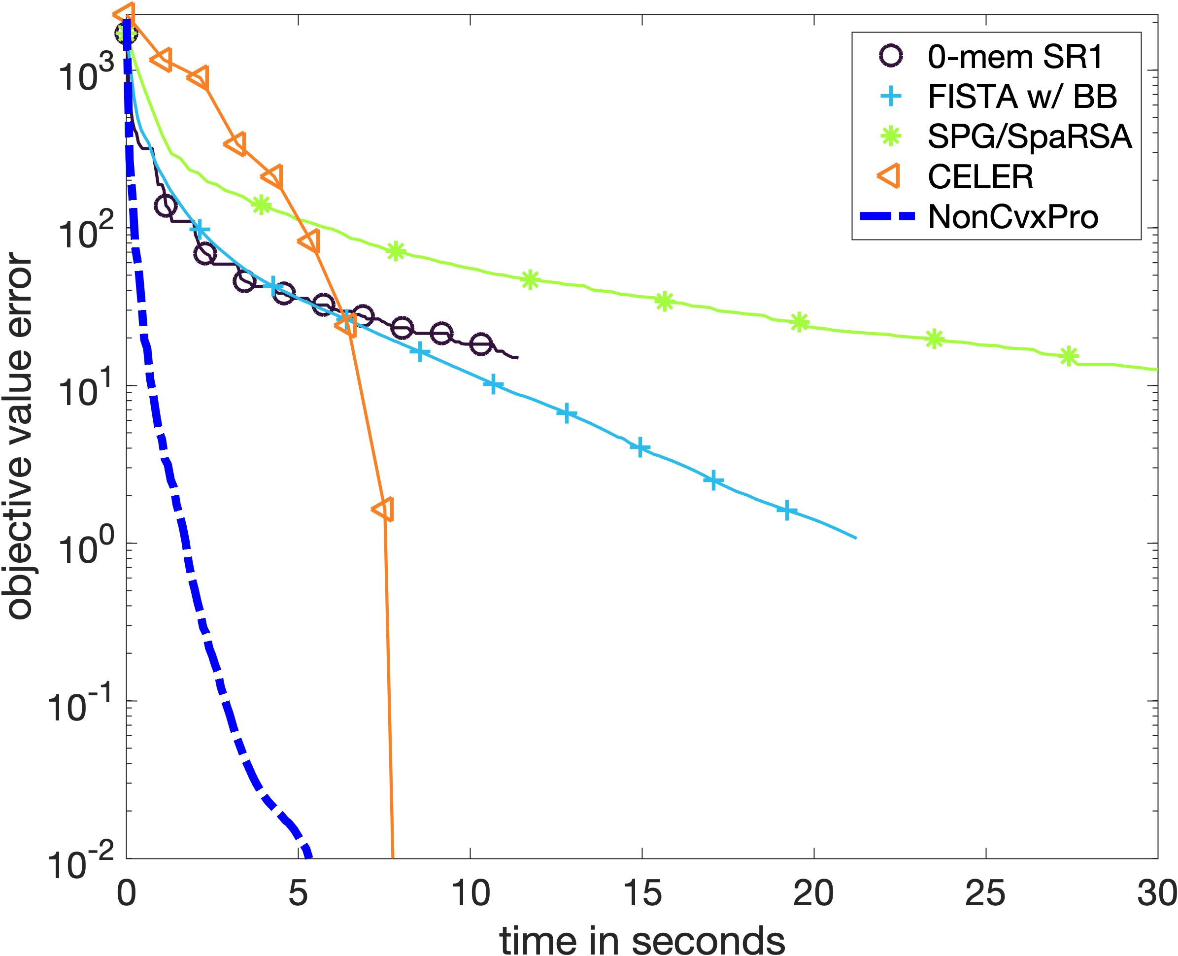
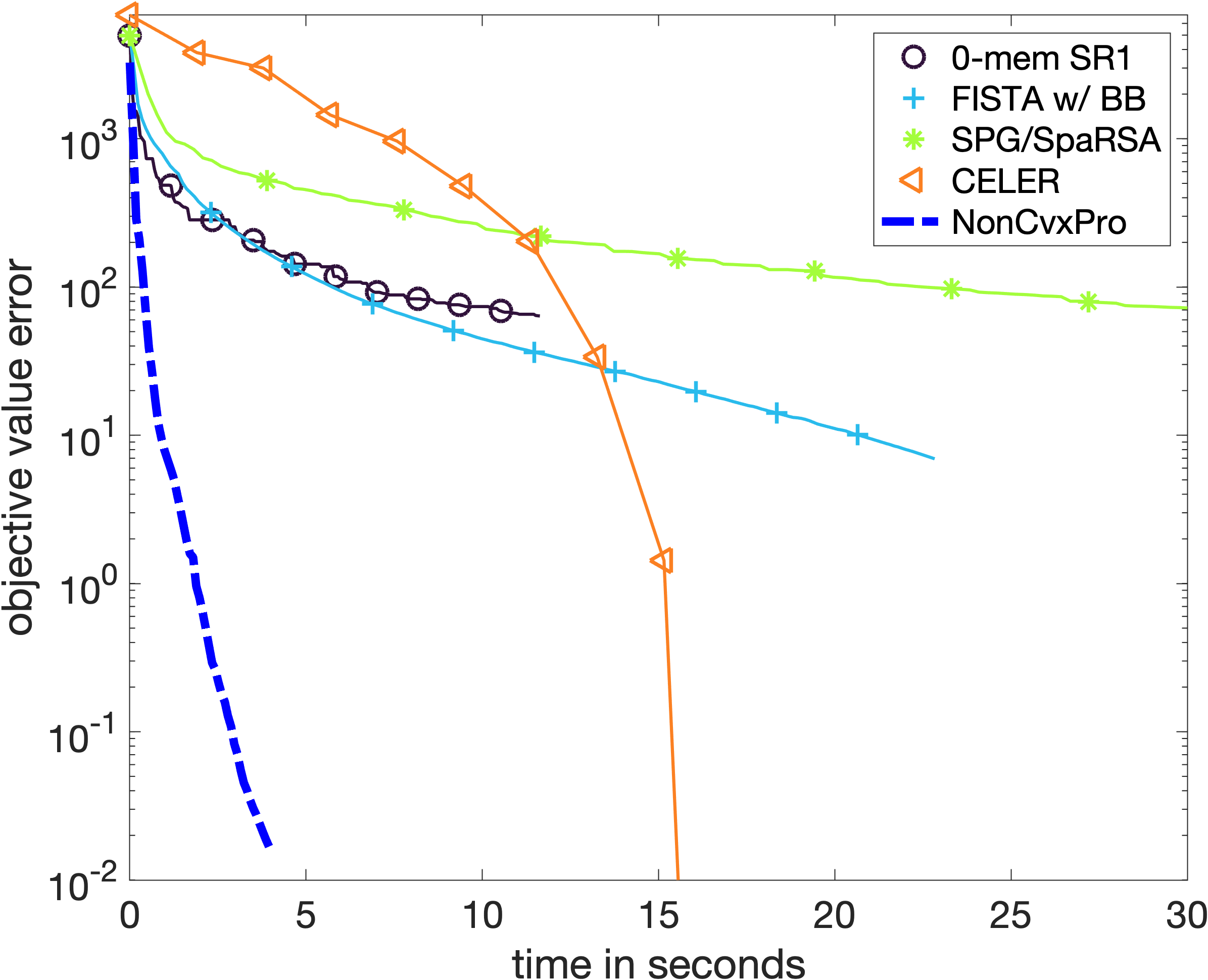
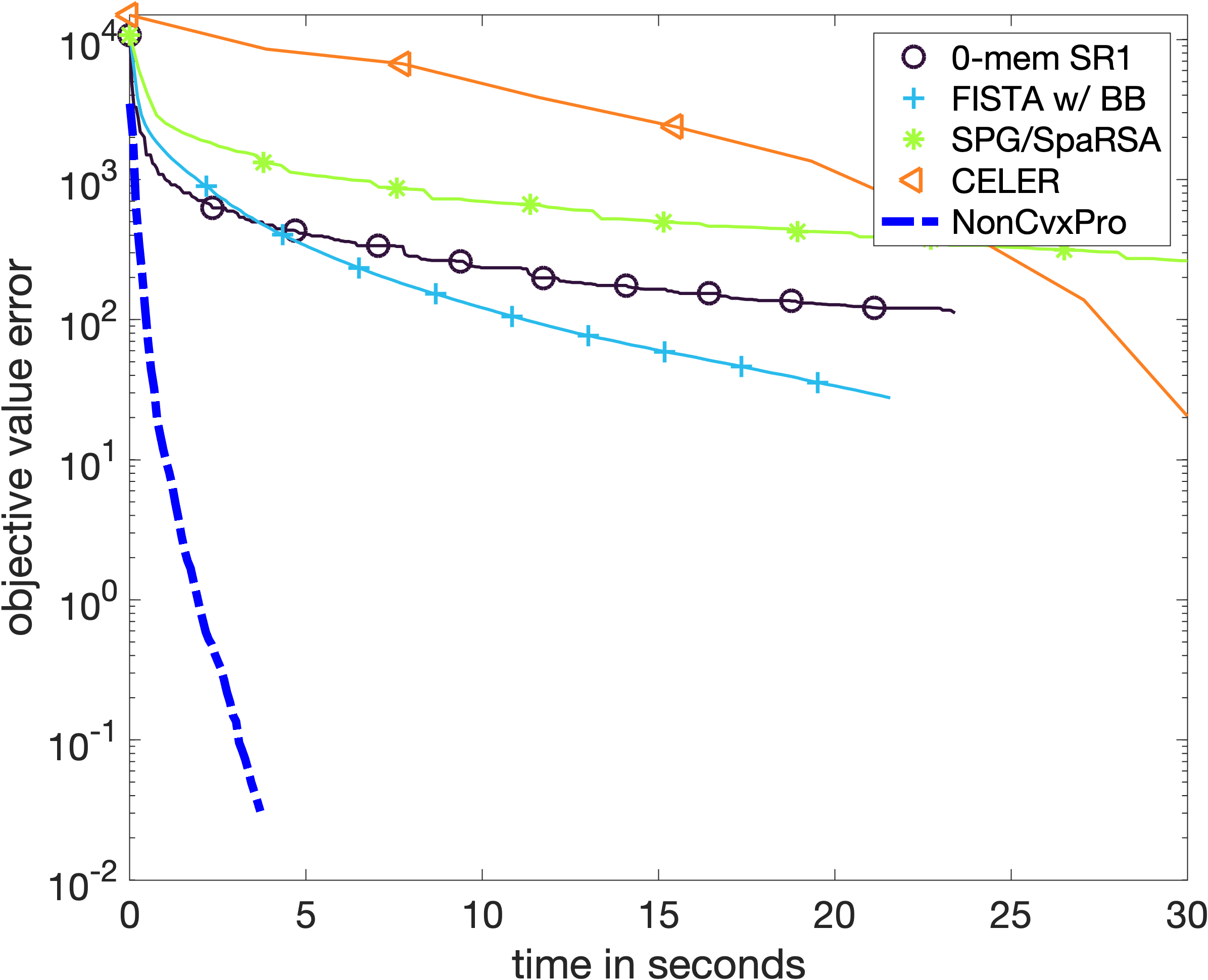
The results are shown in Figure 2 (with further experiments in the appendix). We show comparisons at different regularisation strengths, with $\lambda_{*}$ being the regularisation parameter found by 10 fold cross validation on the mean squared error, and $\lambda_{\max}=|\!|X^{\top}y|\!|_{\infty}$ is the smallest parameter at which the Lasso solution is guaranteed to be trivial.

leukemia (38,7129)
mnist (60000,683)
	$\lambda_{*}$	$\frac{1}{2}\lambda_{\max}$	$\frac{1}{10}\lambda_{\max}$	$\frac{1}{50}\lambda_{\max}$

Figure 2: Lasso comparisons with different regularisation parameters.

4.2 Group Lasso

The multi-task Lasso [29] is the problem (7) where one minimises over $\beta\in\mathbb{R}^{n\times q}$, the observed data is $y\in\mathbb{R}^{m\times q}$ and $R(\beta)=\sum_{j=1}^{n}|\!|\beta^{j}|\!|_{2}$ with $\beta^{j}\in\mathbb{R}^{q}$ denotes the $j^{\mathrm{th}}$ row of the matrix $\beta$ and the loss function is $\frac{1}{2}|\!|y-X\beta|\!|_{F}^{2}$ in terms of the the Frobenius norm.

Datasets.

We benchmark our proposed scheme on a joint MEG/EEG data from [41]. $X$ denotes the forward operator with $n=22494$ source locations, and is constructed from 301 MEG sensors and 59 EEG sensors, so that $m=360$. The observations $y\in\mathbb{R}^{m\times q}$ represent time series measurements at $m$ sensor with $q=181$ timepoints each. The $\beta$ corresponds to the source locations which are assumed to remain constant across time.

Solvers.

We perform a comparison against FISTA with restarts and BB step, the spectral projected gradient method SPG/SpaRSA, and CELER. Since $n$ is much larger than $q$ and $m$, we use for NonCvx-Pro the saddle point formulation (8) where the maximisation is over $\alpha\in\mathbb{R}^{m\times q}$. Computation of $\alpha$ in $\nabla f(v)$ involves solving $(\mathrm{Id}_{m}+\frac{1}{\lambda}X\operatorname{diag}(v^{2})X^{\top})\alpha=y.$, that is, $q$ linear systems each of size $m$.

Experiments.

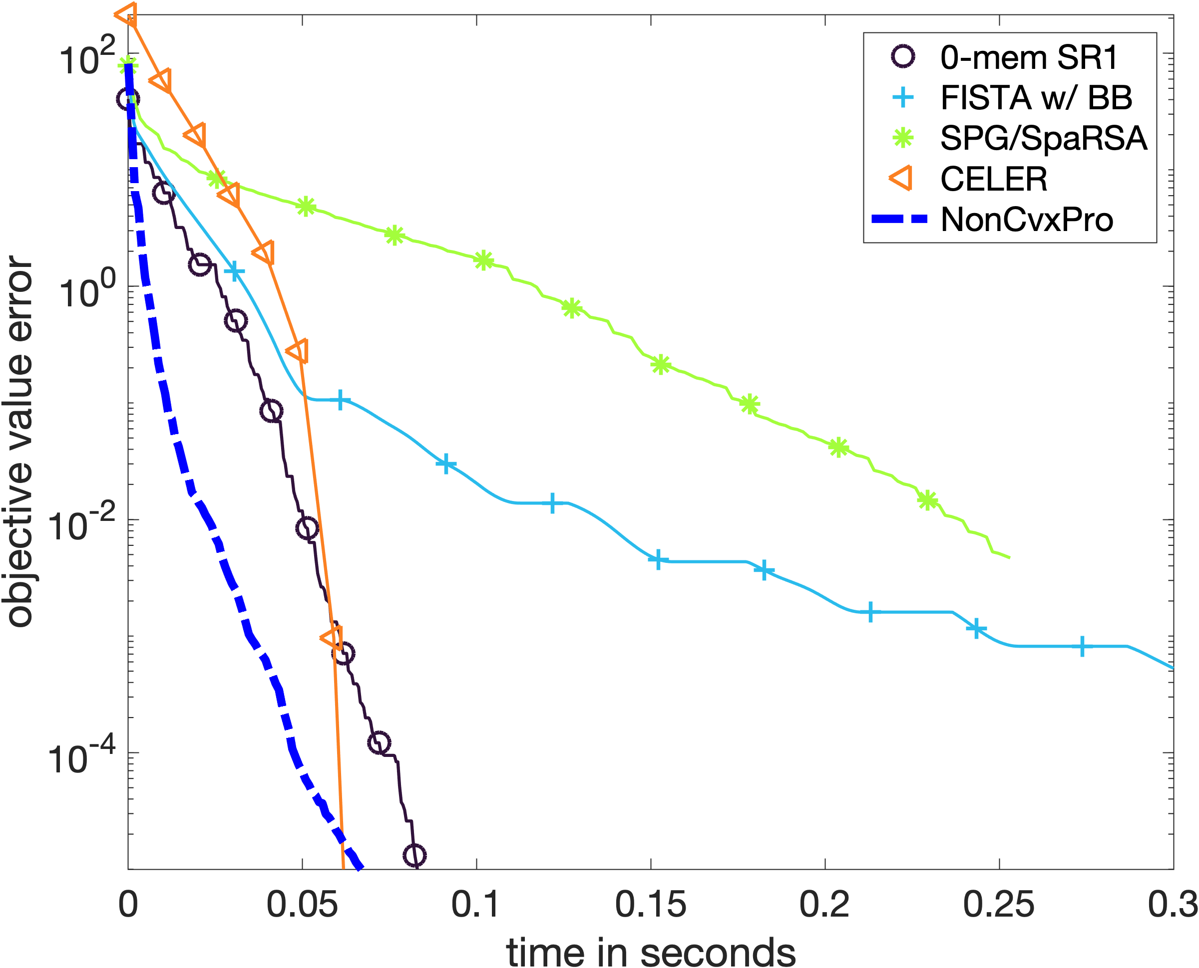
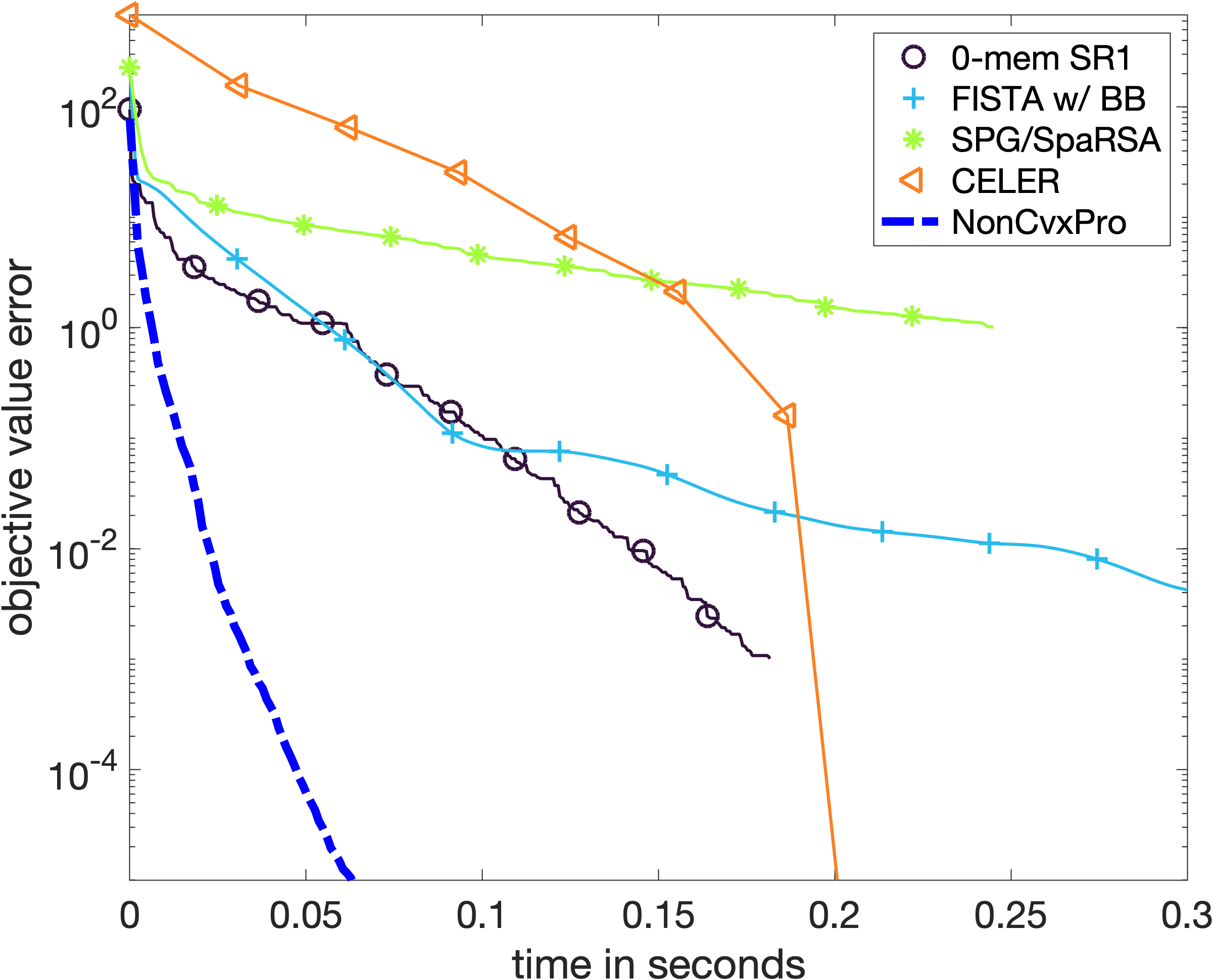
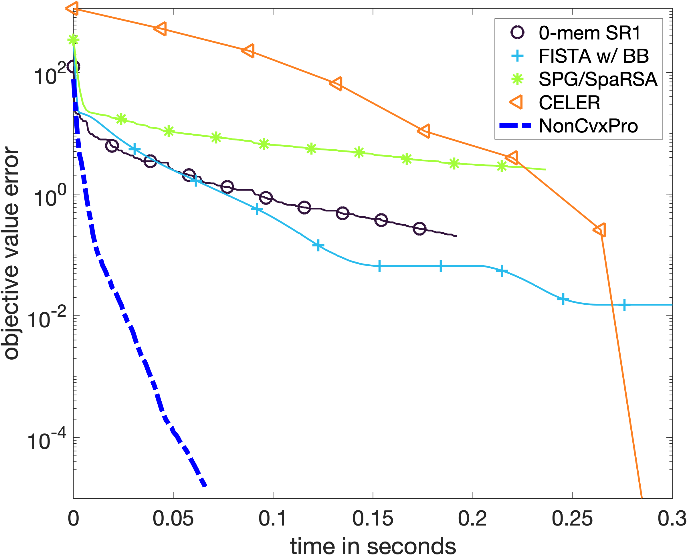
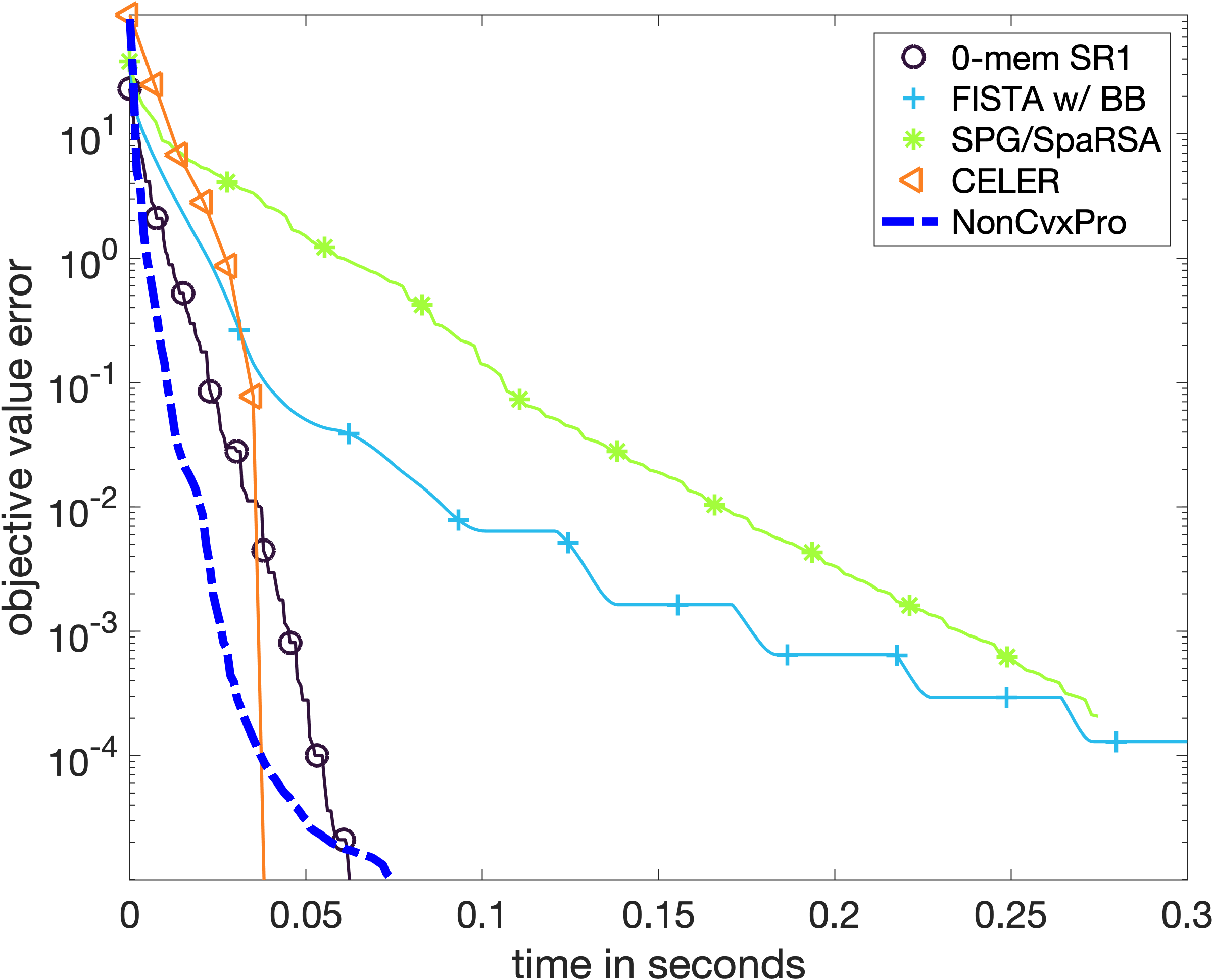
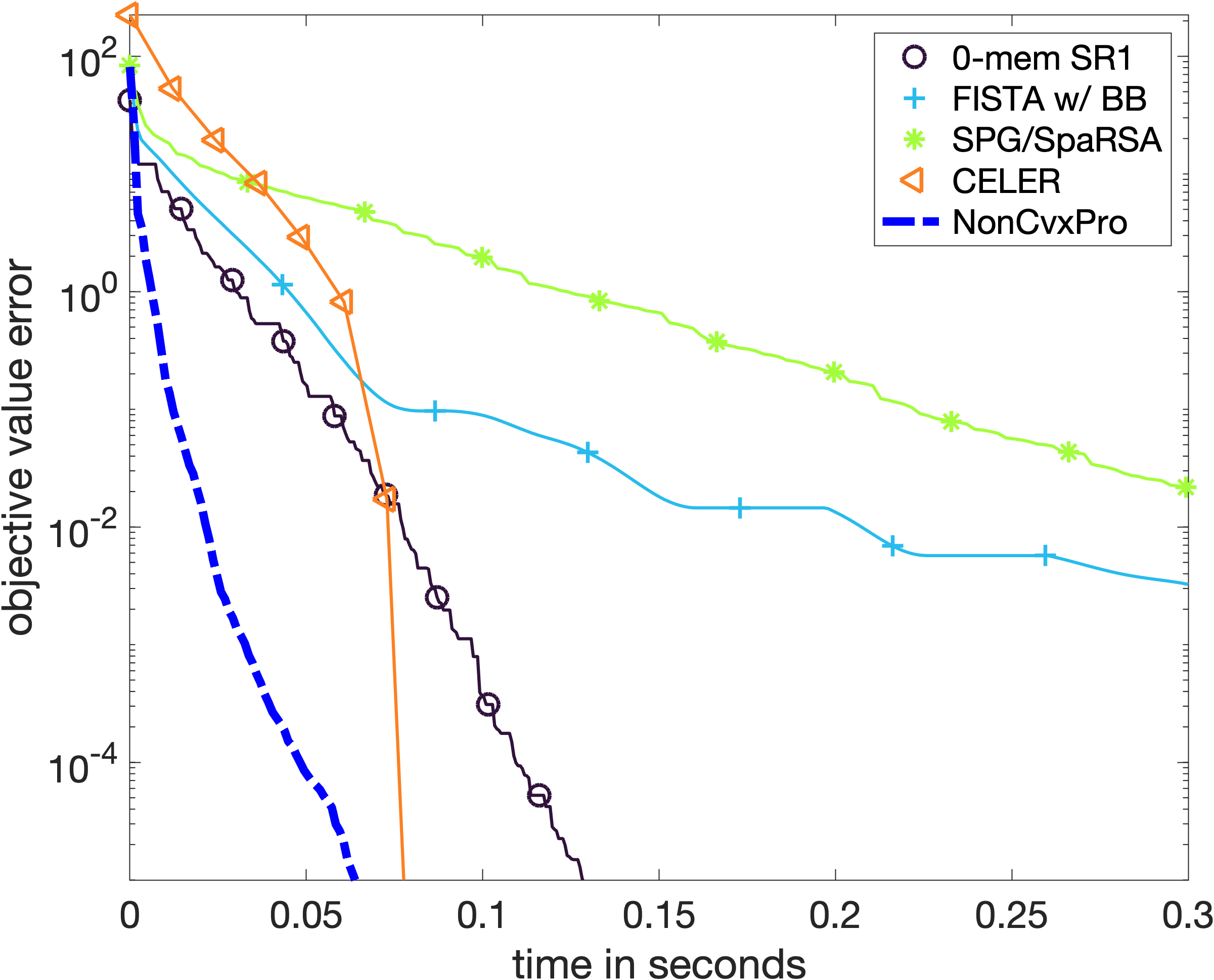
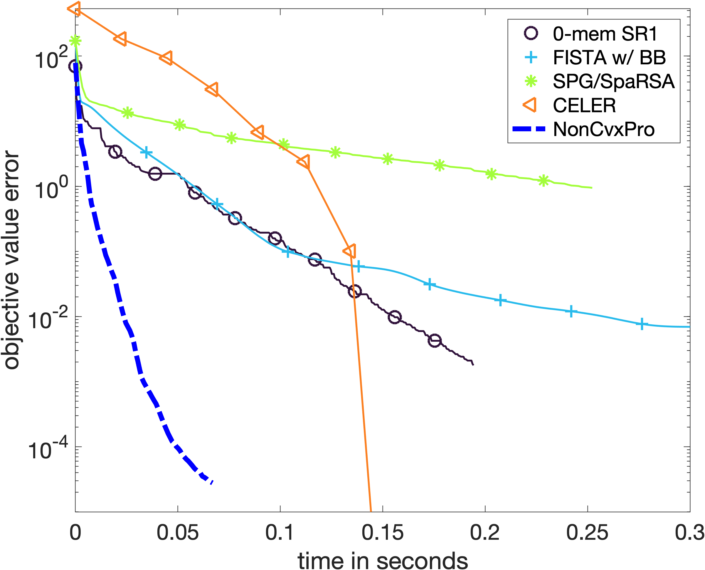
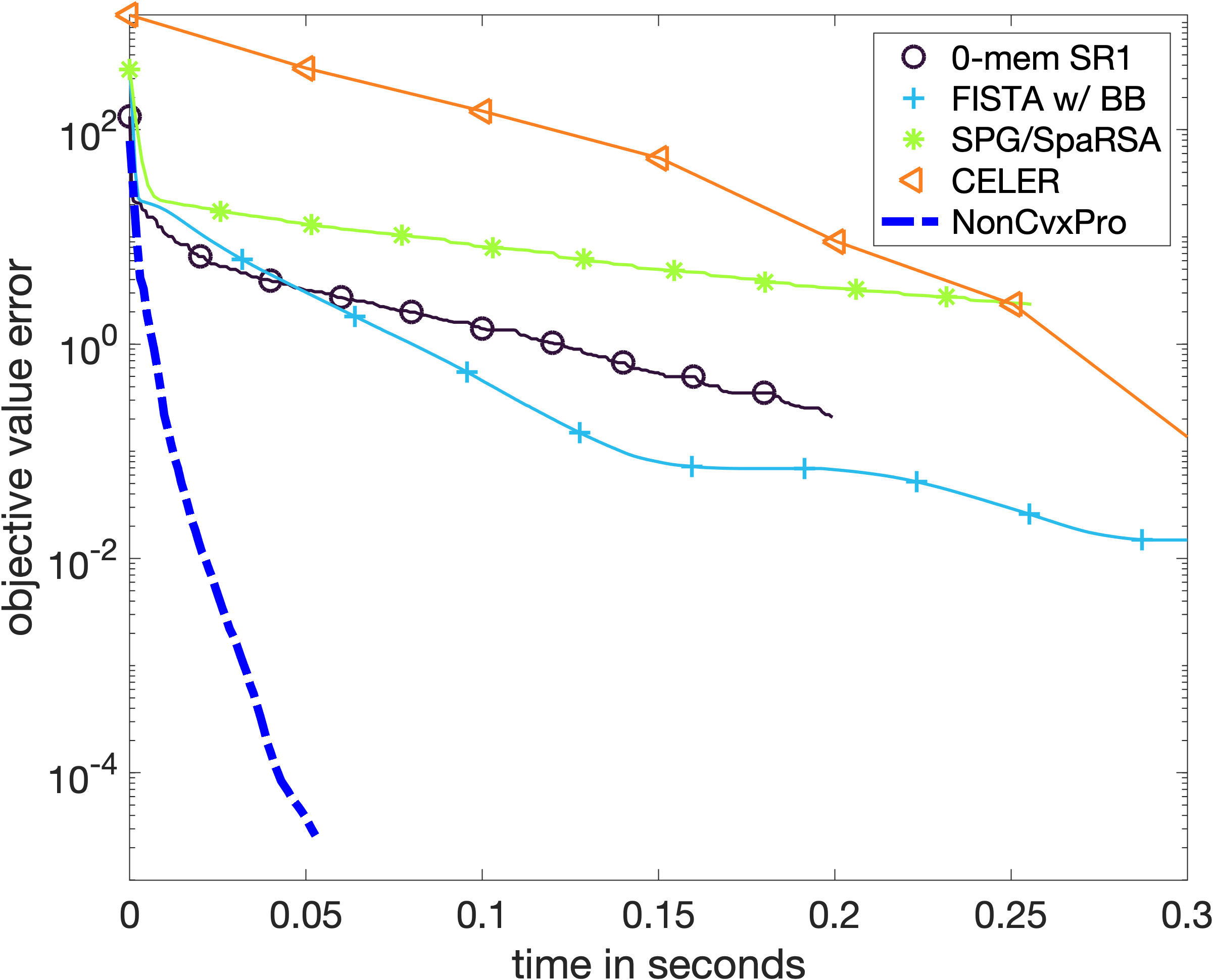
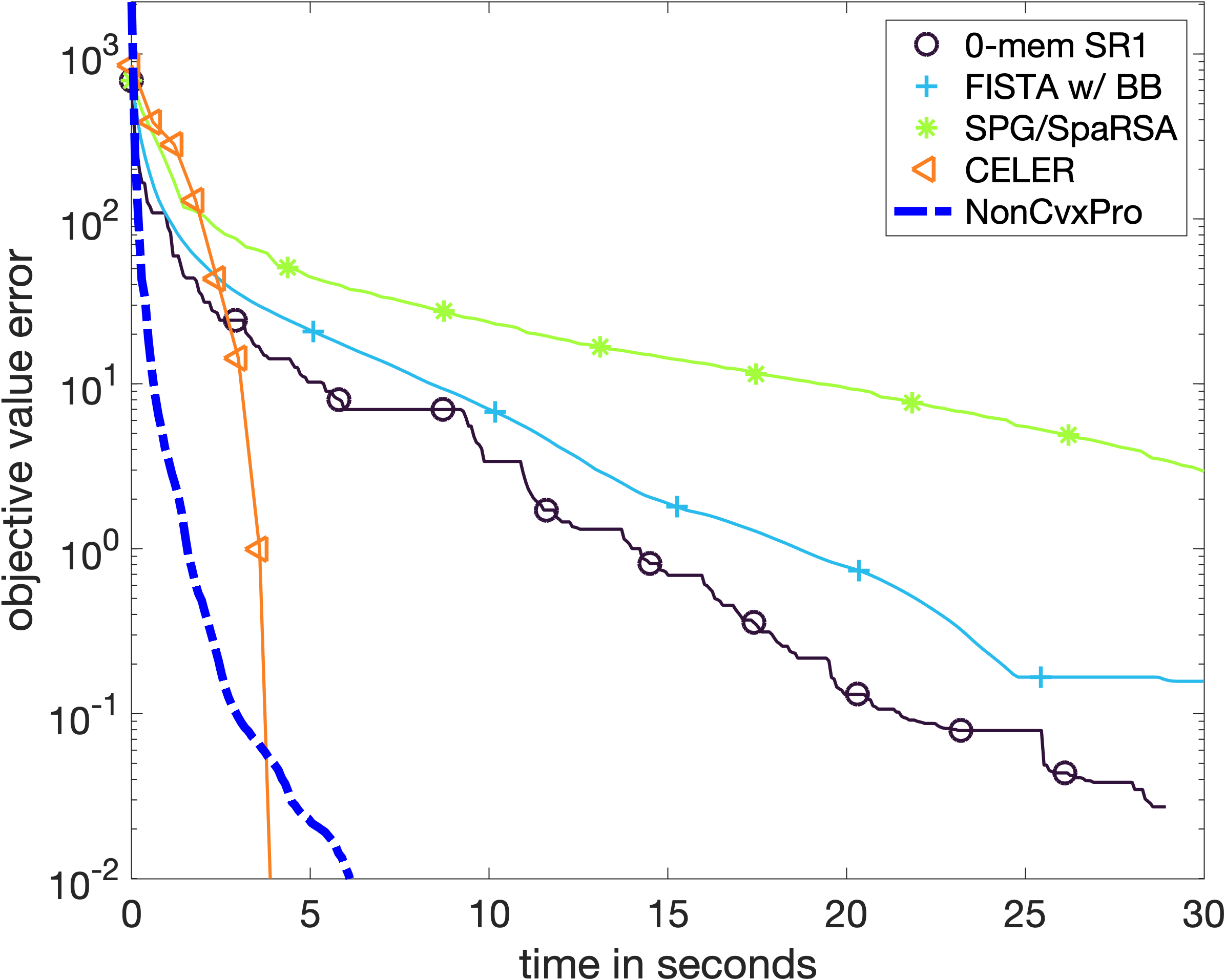
Figure 3 displays the objective convergence plots against running time for different $\lambda$: $\lambda=\lambda_{\max}/r$ with $\lambda_{\max}=\max_{i}|\!|X_{i}^{\top}y|\!|_{2}$ for $r=10,20,50,100$. We observe substantial performance gains over the benchmarked methods: In MEG/EEG problems, the design matrix tends to exhibit high correlation of columns and proximal-based algorithms tend to perform poorly here. Coordinate descent with pruning is known to perform well here when the regularisation parameter large [39], but its performance deteriorates as $\lambda$ increases.

$\lambda=\frac{1}{10}\lambda_{\max}$	$\lambda=\frac{1}{20}\lambda_{\max}$	$\lambda=\frac{1}{50}\lambda_{\max}$	$\lambda=\frac{1}{100}\lambda_{\max}$

Figure 3: Comparisons for multitask Lasso on MEG/EEG data

4.3 Trace norm

In multi-task feature learning [1], for each task $t=1,\ldots,T$, we aim to find $f_{t}:\mathbb{R}^{n}\to\mathbb{R}$ given training examples $(x_{t,i},y_{t,i})\in\mathbb{R}^{n}\times\mathbb{R}$ for $i=1,\ldots,m_{t}$. One approach is to jointly solve these $T$ regression problems by minimising (5) where $R$ is the trace norm (also called “nuclear norm”), $r=T$, $y=\left(y_{t}\right)_{t=1}^{T}$, $\mathcal{A}(B)=\left(X_{t}B_{t}\right)_{t=1}^{T}$ with $X_{t}$ being the matrix with $i^{\mathrm{th}}$ row as $x_{t,i}$ and $B_{t}$ being the $t^{\mathrm{th}}$ column of the matrix $B$. Note that letting $u_{t}\in\mathbb{R}^{n}$ denote the $t^{\mathrm{th}}$ column of $U$, the computation of $U$ in $\nabla f(V)$ involves solving $T$ linear systems $(\lambda\mathrm{Id}_{n}+V^{\top}X_{t}^{\top}X_{t}V)u_{t}=V^{\top}X_{t}^{\top}y_{t}$. Here, the trace norm encourages the tasks to share a small number of linear features.

Datasets.

We consider the three datasets commonly considered in previous works. The Schools dataset from [1] consists of the scores of 15362 students from 139 schools. There are therefore $T=139$ tasks with $15362=\sum_{t}m_{t}$ data points in total, and the goal is to map $n=27$ student attributes to exam performance. The SARCOS dataset [60, 61] has 7 tasks, each corresponding to learning the dynamics of a SARCOS anthropomorphic robot arms. There are $n=21$ features and $m=48,933$ data points, which are shared across all tasks. The Parkinsons dataset [56] which is made up of $m=5875$ datapoints from $T=42$ patients. The goal is to map $n=19$ biomarkers to Parkinson’s disease symptom scores for each patient.

Solvers.

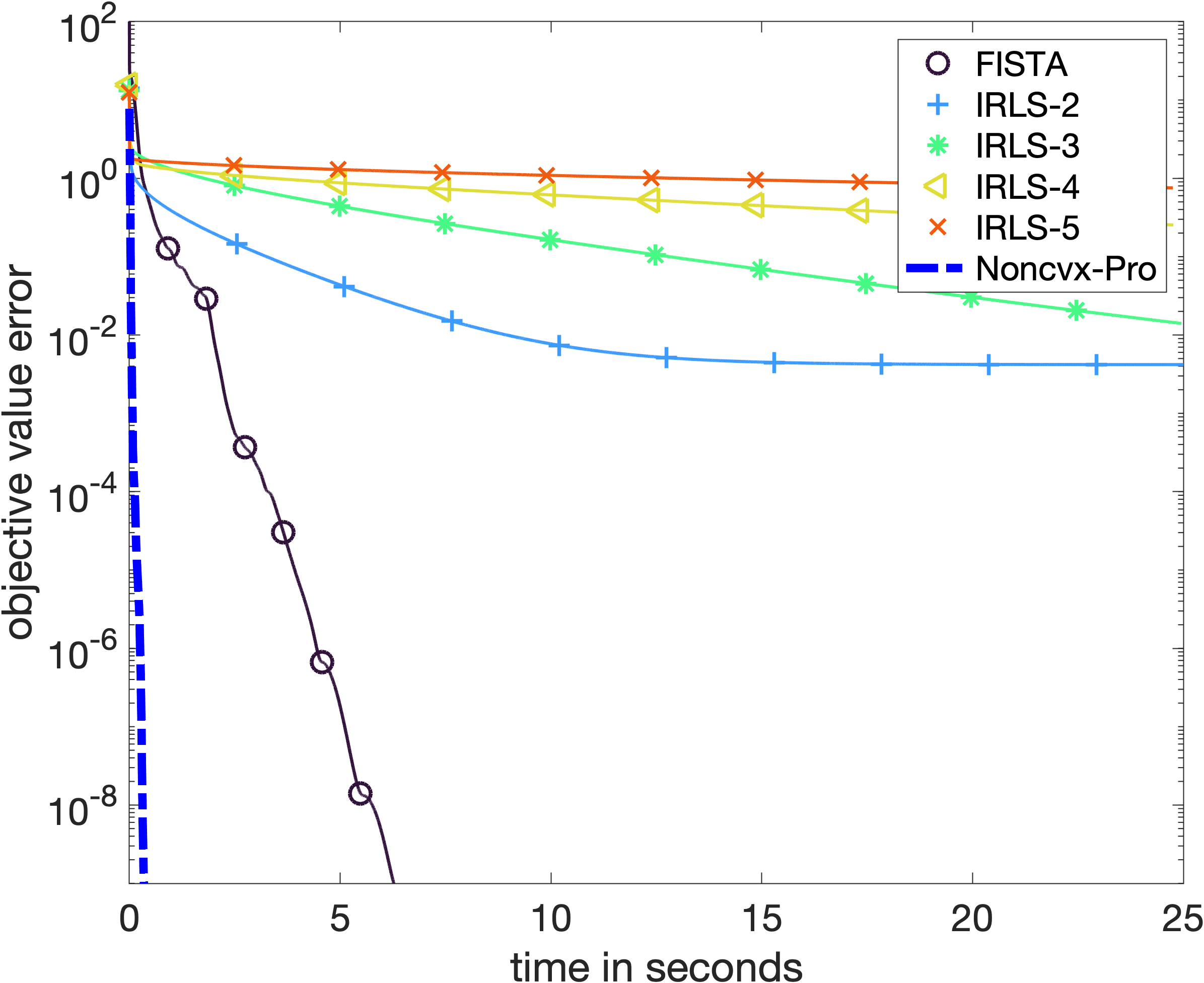
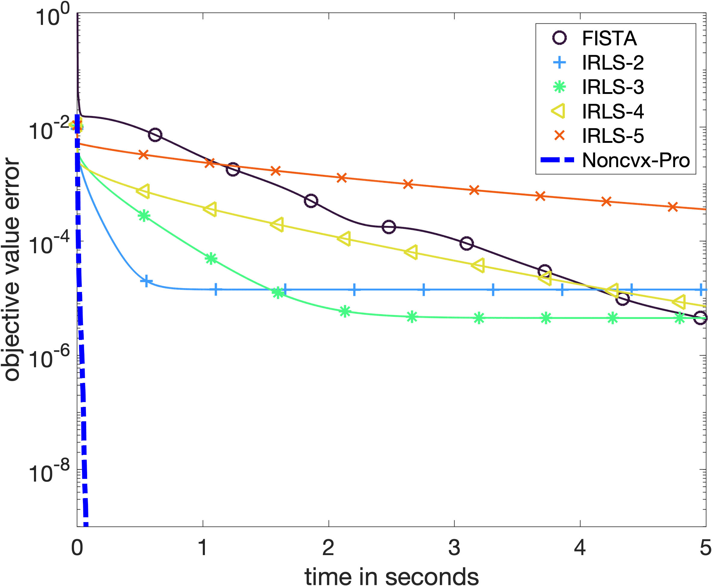
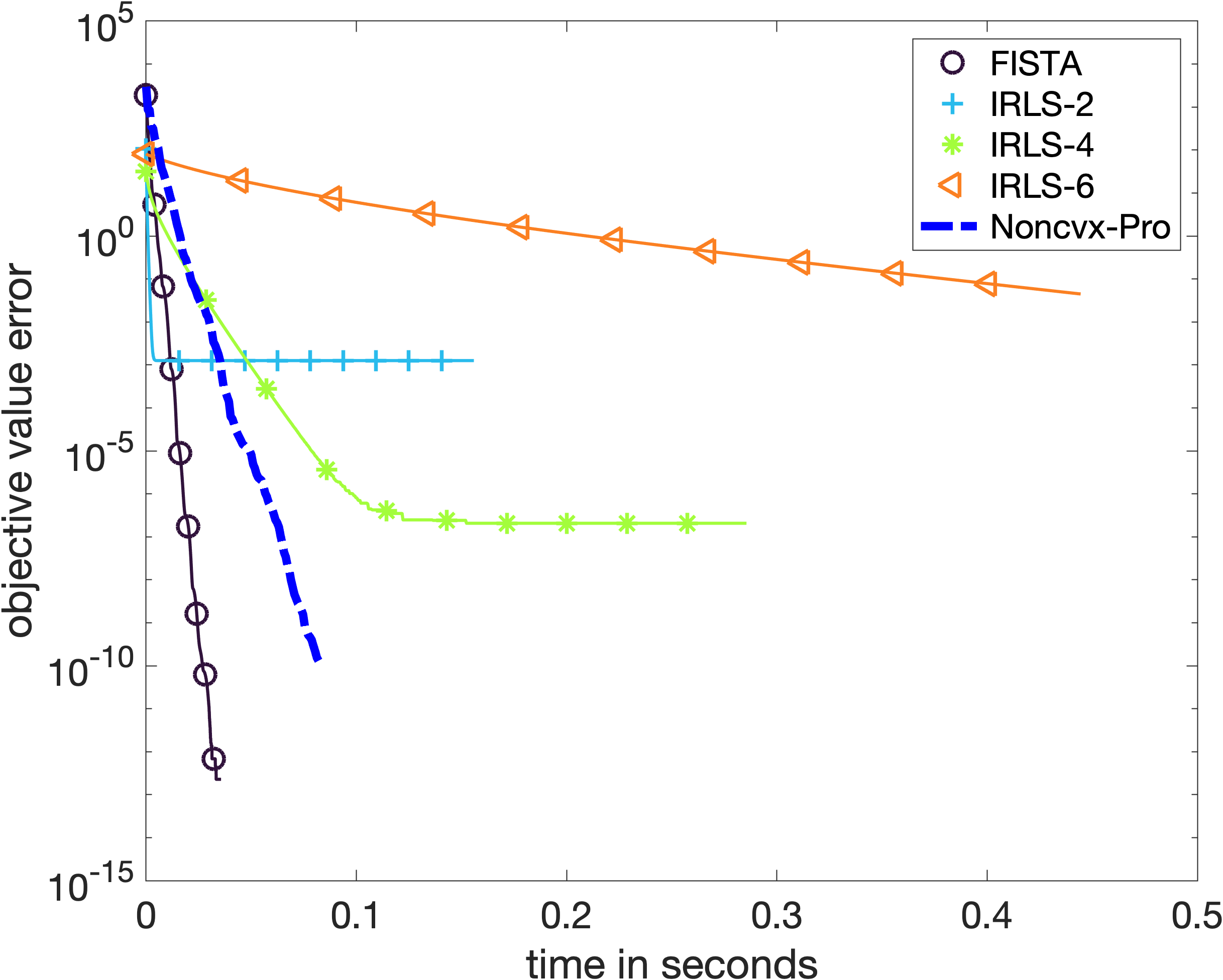
Figure 4 reports a comparison against FISTA with restarts and IRLS. The IRLS algorithm for (5) is introduced in [1] (see also [3]), and applies alternate minimisation after adding the regularisation term $\varepsilon\lambda\operatorname{tr}(Z^{-1})/2$ to (4). The update of $B$ is a simple least squares problem while the update for $Z$ is $Z\leftarrow(BB^{\top}+\varepsilon\mathrm{Id})^{\frac{1}{2}}$. Our nonconvex approach has the same per-iteration complexity as IRLS, but one advantage is that we directly deal with (5) without any $\varepsilon$ regularisation.

Remark 4.

Quad-variational mentioned in Section 4.1 does not extend to the trace norm case, since the function $g$ would be minimised over $\mathbb{S}_{+}^{n}$, for which the application of L-BFGS-B is unclear. For this reason, bilevel formulations for the trace norm [48] have been restricted to the use of first order methods.

Schools	Parkinsons	SARCOS

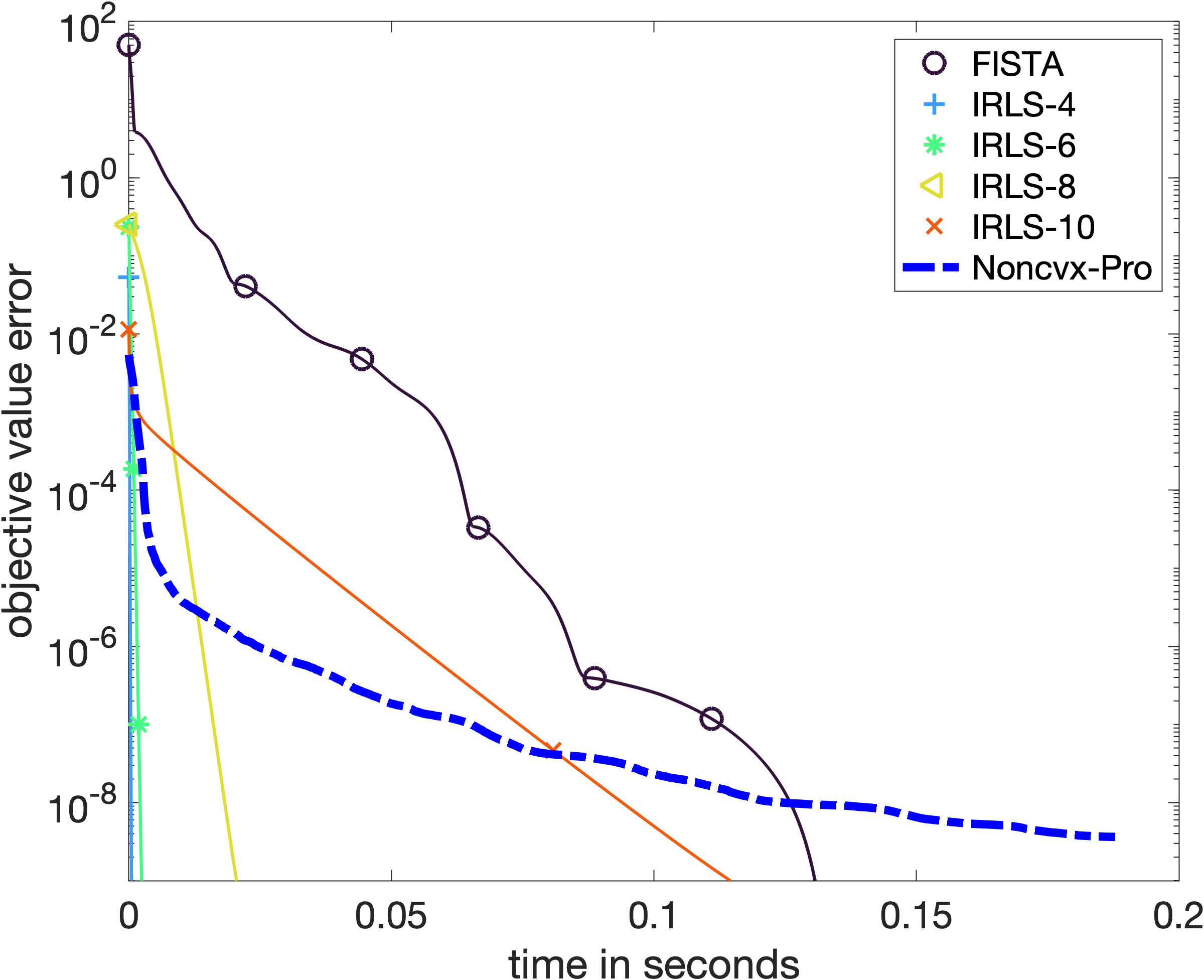
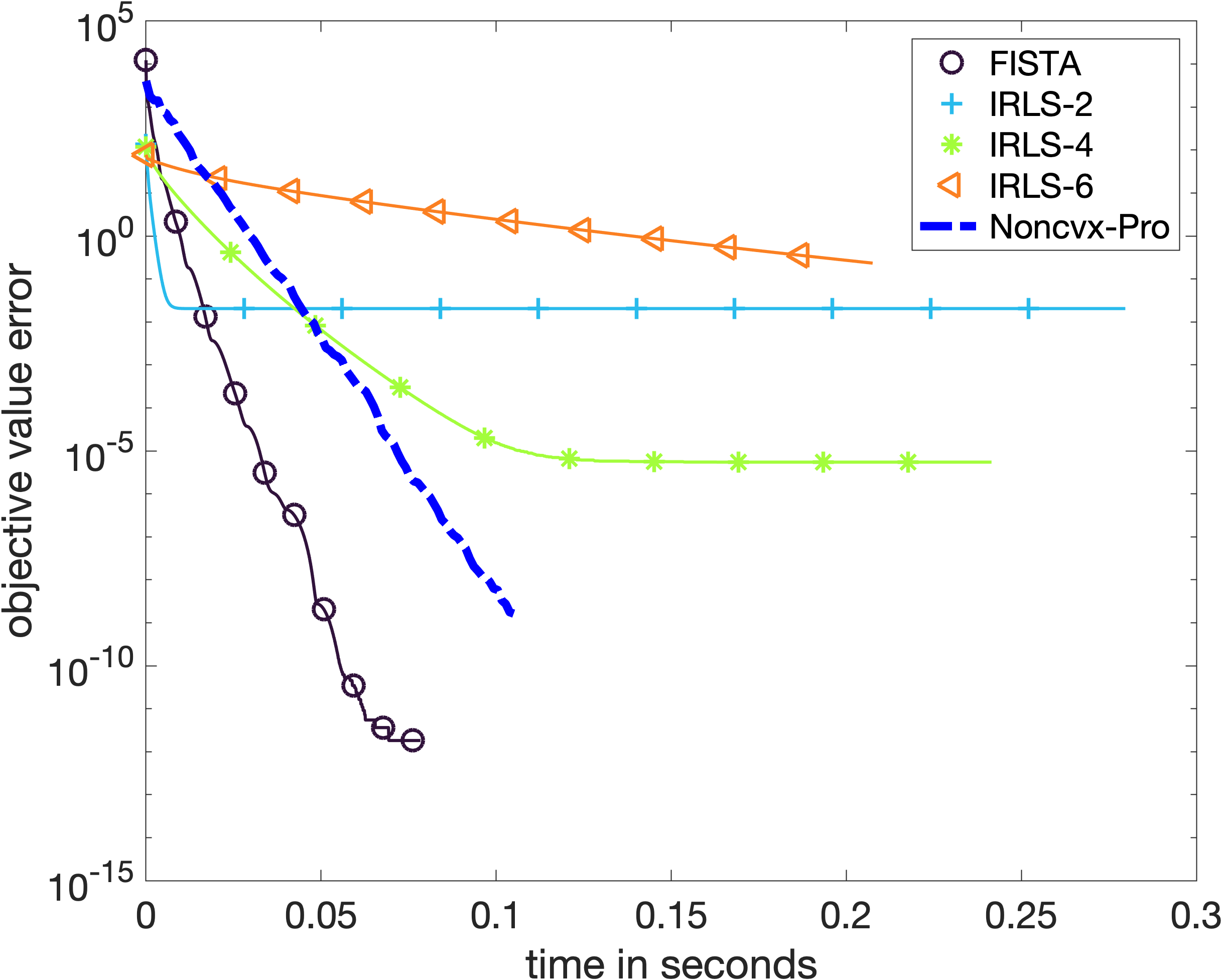
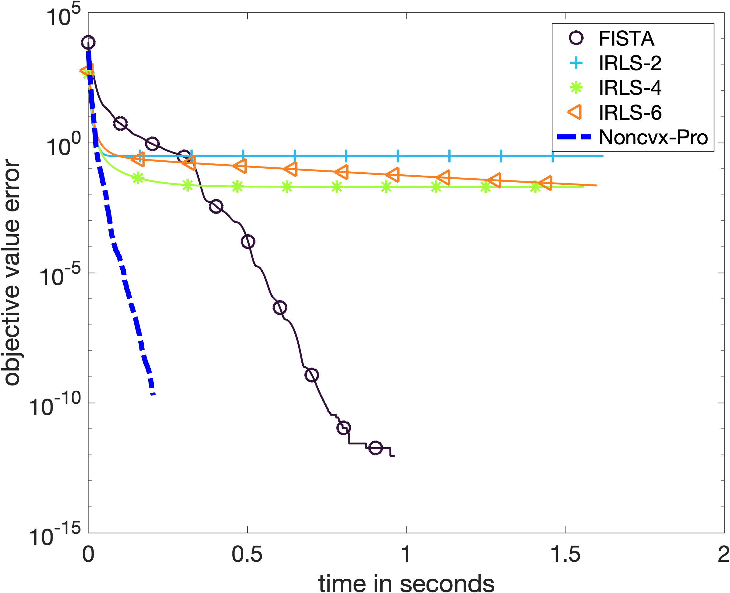
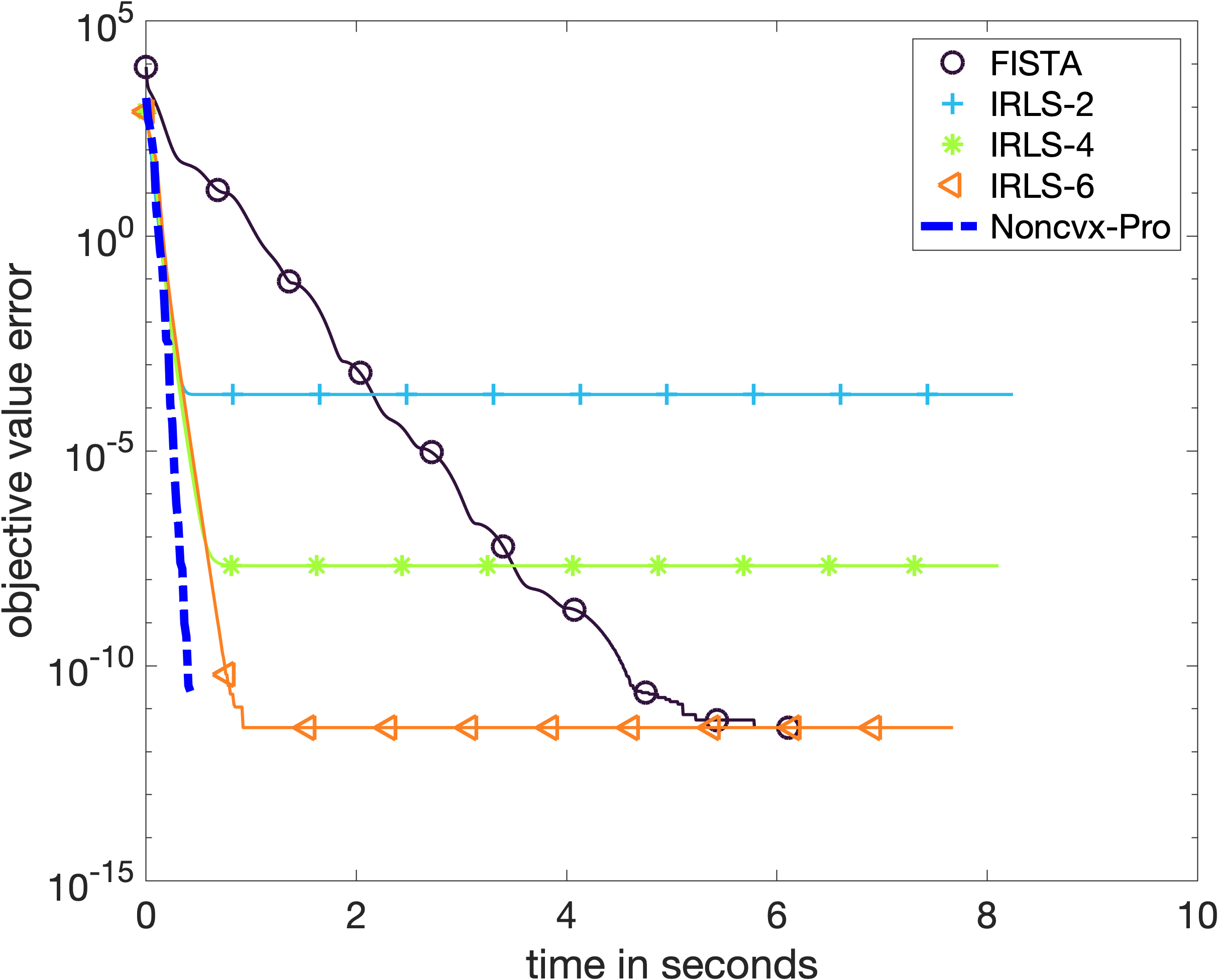
Figure 4: Comparisons for multi-task feature learning, IRLS-d corresponds to IRLS with $\varepsilon=10^{-d}$.

Experiments.

For each dataset, we compute the regularisation parameter $\lambda_{*}$ by 10-fold cross-validation on the RMSE averaged across 10 random splits. Then, with this regularisation parameter, we compare Non-convex-pro, FISTA and IRLS with different choices of $\varepsilon$. The convergence plots are show in Figure 4. We observe substantial computational gains for the Schools and Parkinson’s dataset. For the SARCOS dataset, IRLS performed the best, and even though Nonconvex-pro is comparatively less effective here, although we remark that the number of tasks is much smaller ($T=7$) and the recorded times are much shorter (less than 0.2s). Further numerical illustrations with synthetic data are shown in the appendix – our method is typically less sensitive to problem variations.

4.4 Constraint Group Lasso and Optimal Transport

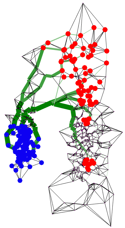
A salient feature of our method is that it can handle arbitrary small regularization parameter $\lambda$ and can even cope with the constrained formulation, when $\lambda=0$, which cannot be tackled by most state of the art Lasso solvers. To illustrate this, we consider the computation of an Optimal Transport (OT) map, which has recently gained a lot of attention in ML [47]. We focus on the Monge problem, where the ground cost is the geodesic distance on either a graph or a surface (which extends original Monge’s problem where the cost is the Euclidean distance). This type of OT problems has been used for instance to analyze and process brain signals in M/EEG [30], for application in computer graphics [55] and is now being applied to genomic datasets [54]. As explained for instance in [53, Sec.4.2], the optimal transport between two probability measures $a$ and $b$ on a surface can be computed by advecting the mass along a vector field $v(x)\in\mathbb{R}^{3}$ (tangent to the surface) with minimum vectorial $L^{1}$ norm $\int|\!|v(x)|\!|\mathrm{d}x$ (where $\mathrm{d}x$ is the surface area measure) subject to the conservation of mass $\text{div}(v)=a-b$. Once discretized on a 3-D mesh, this boils down to solving a constrained group Lasso problem $(\mathcal{P}_{0})$ where $\beta_{g}\in\mathbb{R}^{3}$ is a discretization of $v(z_{g})$ at some vertex $z_{g}$ of the mesh, $X$ is a finite element discretization of the divergence using finite elements and $y=a-b$. The same applies on a graph, in which case the vector field is aligned with the edge of the graph and the divergence is the discrete divergence associated to the graph adjacency matrix, see [47]. This formulation is often called “Beckmann problem”.

Datasets.

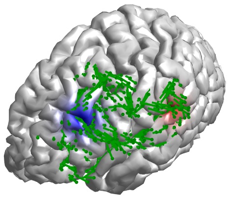
We consider two experiments: (i) following [30] on a 3-D mesh of the brain with $n=20000$ vertices with localized Gaussian-like distributions $a$ and $b$ (in blue and red), (ii) a 5-nearest neighbors graph in a 7-dimensional space of gene expression (corresponding to 7 different time steps) of baker’s yeast, which is the dataset from [20]. The $n=614$ nodes correspond to the most active genes (maximum variance across time) and this results in a graph with 1927 edges. The distributions are synthetic data, where $a$ is a localized source whereas $b$ is more delocalized.

Solvers.

We test our method against two popular first order schemes: the Douglas-Rachford (DR) algorithm [37, 16] (DR) and the primal-dual scheme of [14]. DR is used in its dual formulation (the Alternating Direction Method of Multipliers – ADMM) but on a re-parameterized problem in [55]. The details of these algorithms are given in Appendix E.

Experiments.

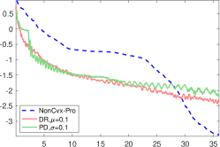
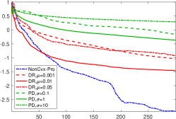
Figure 5 shows the solution of this Beckmann problem in these two settings. While DR has the same complexity per iteration as the computation of the gradient of $f$ (resolution of a linear system), a chief advantage of PD is that it only involves the application of $X$ and $X^{\top}$ et each iterations. Both DR and PD have stepping size parameters (denoted $\mu$ and $\sigma$) which have been tuned manually (the rightmost figure shows two other sub-optimal choices of parameters). In contrast, our algorithm has no parameter to tune and is faster than both DR and PD on these two problems.

Figure 5: Resolution of Beckmann problem on a graph (left) and a 3-D mesh (right). The probability distributions $a$ and $b$ are displayed in blue and red and the optimal flow $\beta$ is represented as green segments (on the edge of the graph and on the faces of the mesh). The convergence curves display the decay of $\log_{10}(|\!|\beta_{t}-\beta^{\star}|\!|_{1})$ during the iterations of the algorithms (DR=Douglas-Rachford, PD=Primal-Dual) as a function of time $t$ in second.

5 Conclusion

Most existing approaches to sparse regularisation involve careful smoothing of the nonsmooth term, either by proximal operators or explicit regularisation as in IRLS. We propose a different direction: a simple reparameterization leads to a smooth optimisation problem, and allows for the use of standard numerical tools, such as BFGS. Our numerical results demonstrate that this approach is versatile, effective and can handle a wide range of problems.

We end by making some remarks on possible future research directions. The application of our method to other loss functions requires the use of an inexact solver for the inner problems, and controlling the impact of its approximation is an interesting avenue for future work. Furthermore, it is possible that one can obtain further acceleration by combining with screening rules or active set techniques.

Appendix A Pseudocode for gradient descent implementation

For concreteness, we write down in Algorithm 1 the gradient descent algorithm for solving

$$\min_{\beta\in\mathbb{R}^{n}}\frac{1}{2\lambda}|\!|X\beta-y|\!|_{2}^{2}+|\!|\beta|\!|_{1},$$

where we recall that $X\in\mathbb{R}^{m\times n}$. The choice of $\lambda=0$ corresponds to the Basis-pursuit setting. Note that $\nabla f(\beta_{t})=g_{t}$ is computed either as in line 5 or line 9 of the algorithm and one can use these computations for any gradient based algorithm (e.g. BFGS). Note also that this is simply gradient descent on a smooth function, and one can apply typical methods to choosing the stepsize $\gamma_{k}$, such as the Barzilai-Borwein stepsize [5].

1 initialization $v_{0}\in\mathbb{R}^{n}$ (with no zero entries), stepsize $\gamma_{t}>0$;

Result: $\beta_{t}$

2 while not converged do

3       if $n\leqslant m$ and $\lambda>0$ then

4             $u_{t}=-\left(\operatorname{diag}(v_{t})X^{\top}X\operatorname{diag}(v_{t})+\lambda\mathrm{Id}\right)^{-1}\left(v_{t}\odot X^{\top}y\right)$;

5             $g_{t}=v_{t}\odot v_{t}+\frac{1}{\lambda}u_{t}\odot{X^{\top}(Xu_{t}\odot v_{t}-y)}$;

6             $\beta_{t}=u_{t}\odot v_{t}$;

7            

8      else

9             $\alpha_{t}=-\left(X\operatorname{diag}(v_{t}\odot v_{t})X^{\top}+\lambda\mathrm{Id}\right)^{-1}y$;

10             $g_{t}=v_{t}\odot v_{t}-v_{t}\odot|X^{\top}\alpha_{t}|^{2}$;

11             $\beta_{t}=-v_{t}\odot v_{t}\odot X^{\top}\alpha_{t}$;

12            

13       end if

14      $v_{t+1}=v_{t}-\gamma_{t}g_{t}$

15 end while

Algorithm 1 Gradient descent implementation of Ncvx-Pro for solving Lasso.

Appendix B Proofs and additional results for Section 2

Proof to Theorem 1.

To show that i) implies ii), recall that a convex, proper and lower semicontinuous function $-\varphi$ can be written in terms of its convex conjugate which has domain $\mathbb{R}_{-}^{d}$. By writing $\beta^{2}\triangleq\beta\odot\beta$, using the definition of $R$, we have

$$-R(\beta^{2}) =-\varphi(\beta^{2})=\sup_{v\leqslant 0}\langle\beta^{2},\,v\rangle-(-\varphi)^{*}(v)=-\inf_{u\geqslant 0}\langle\beta^{2},\,u\rangle+(-\varphi)^{*}(-u).$$

which is ii) with $\psi(u)\triangleq(-\varphi)^{*}(-u)$ as required.

Conversely, if $R$ is of the form in ii), then

$$R(\beta)=\inf_{u\in\mathbb{R}_{+}^{n}}\langle u,\,\beta^{2}\rangle+\psi(u)=-\sup_{u\in\mathbb{R}_{+}^{n}}-\langle u,\,\beta^{2}\rangle-\psi(u),$$

so $R(\beta)=-\psi^{*}(-\beta\odot\beta)$ and $-\psi^{*}(-\cdot)$ is clearly a proper, upper semicontinuous, concave function.

For the expression of $\psi$ when $R$ is a norm,from the above, we know that $\psi=(-\varphi)^{*}(-z)$, and recall that for any norm, $R(\beta)=\max_{R^{*}(w)\leqslant 1}\langle w,\,\beta\rangle$. So,

$$\psi(z) =\max_{u\geqslant 0}\langle-u,\,z\rangle+\varphi(u)$$

$$=\max_{\beta}\langle-\beta^{2},\,z\rangle+\varphi(\beta^{2})=\max_{\beta}\langle-\beta^{2},\,z\rangle+R(\beta)$$

$$=\max_{\beta}\langle-z,\,\beta^{2}\rangle+\max_{R^{*}(w)\leqslant 1}\langle\beta,\,w\rangle=\max_{R^{*}(w)\leqslant 1}\frac{1}{4}\sum_{i}\frac{w_{i}^{2}}{z_{i}},$$

where in the line, we swapped the two maximums and used the optimality condition over $\beta$ which is $2\beta\odot z=w$. That is, $h(\eta)=2\psi(-\frac{1}{2\eta})=\max_{R^{*}(w)\leqslant 1}\sum_{i}w_{i}^{2}\eta_{i}$.

To derive the identity for $R(\beta)^{2}$, by the Cauchy-Schwarz inequality

$$R(\beta)^{2}=\sup_{R^{*}(w)\leqslant 1}|\langle\beta,\,w\rangle|^{2}\leqslant\sup_{R^{*}(w)\leqslant 1}\left(\sum_{i}{\beta_{i}^{2}}\eta_{i}\right)\left(\sum_{i}\frac{w_{i}^{2}}{\eta_{i}}\right)=4\psi(\eta)\sum_{i}{\beta_{i}^{2}}\eta_{i}$$

for all $\eta>0$. Therefore,

$$R(\beta)^{2} \leqslant\inf_{\eta\geqslant 0,\psi(\eta)\leqslant\frac{1}{4}}\sum_{i}{\beta_{i}^{2}}\eta_{i}$$

$$=\sup_{\lambda>0}\inf_{\eta\geqslant 0}\lambda(\psi(\eta)-\frac{1}{4})+\sum_{i}{\beta_{i}^{2}}\eta_{i}$$

$$=\sup_{\lambda>0}-\frac{\lambda}{4}+\lambda R(\beta/\sqrt{\lambda})=\sup_{\lambda>0}-\frac{\lambda}{4}+\sqrt{\lambda}R(\beta)=R(\beta)^{2}.$$

where we used the identity $\lambda R(\beta/\sqrt{\lambda})=\sum_{i}\beta_{i}^{2}\eta_{i}+\lambda\psi(\eta)$ and the fact that $R$ is one positive homogeneous.

∎

We derive some properties of the function $h$:

Lemma 1.

Consider the function $\varphi$ and $\psi$ from Theorem 1. If $\varphi:[0,\infty)\to[L,U]$, where $L>-\infty$ and $U\in\mathbb{R}\cup\{+\infty\}$, then $\psi$ is an decreasing function with domain contained in $[0,\infty)$, taking values in $[L,U]$. If $R$ is coercive, then $\lim_{|\!|z|\!|\to 0}\psi(z)=+\infty$.

Proof to Lemma 1.

Let $\varphi:[0,\infty)\to[L,U]$, where $L>-\infty$ and $U\in\mathbb{R}\cup\{+\infty\}$. We describe the properties of the function $\psi(z)=(-\varphi)^{*}(-z)=\sup_{u\geqslant 0}\langle z,\,-u\rangle+\varphi(u)$.

• $\mathrm{dom}(\psi)\subset[0,\infty)$: since $\varphi$ is bounded below, it is clear that for $z<0$, $\sup_{u\geqslant 0}\langle z,\,-u\rangle+\varphi(u)=+\infty$.

• $\psi(0)=\sup_{u\geqslant 0}\varphi(u)=U$.

• Suppose $M\triangleq\sup\left\{v\;\backslash\;v\in\partial\varphi(u),u\geqslant 0\right\}<\infty$. Then, for all $z\geqslant M$, $-z+\partial\varphi(u)<0$ for all $u\geqslant 0$ and hence, $\psi(z)=\varphi(0)\geqslant L$. Therefore, $\psi$ takes values in $[L,U]$. So, if $M$ is finite, then one can restrict the optimisation over $z$ to values in $[0,M]$.

• $\psi$ is decreasing: By Danskin’s theorem [8, Prop. B.25], for $z\in\left\{v\;\backslash\;v\in\partial\varphi(u),u\geqslant 0\right\}$,

  $$\partial\psi(z)=\left\{-u\;\backslash\;u\in\operatorname{argmin}_{u\geqslant 0}\langle u,\,-z\rangle+\varphi(u)\right\}\subset(-\infty,0).$$

∎

B.1 Functions on matrices

We have the following result for matrix valued functions. Let $\mathbb{S}^{n}_{+}$ denote the set of symmetric positive semidefinite matrices.

Theorem 4.

Let $R:\mathbb{R}^{n\times m}\to\mathbb{R}$. The following are equivalent

• $R(B)=\varphi(BB^{\top})$ where $\varphi$ is a proper concave upper semi-continuous function with domain $\mathbb{S}^{n}_{+}$.

• There exists a convex function $\psi$ such that $R(B)=\min_{Z\in\mathbb{S}^{n}_{+}}\operatorname{tr}(B^{\top}ZB)+\psi(Z).$

Moreover, we have $\psi(Z)=(-\varphi)^{*}(-Z)$. If $R$ is a norm, then $\psi$ can be written as

$$\psi(Z)=\max_{R^{*}(W)\leqslant 1}\frac{1}{4}\operatorname{tr}(W^{\top}Z^{-1}W).$$ (13)

Moreover,

$$R(B)^{2}=\inf_{Z\in\mathbb{S}^{n}_{+}}\left\{\operatorname{tr}(B^{\top}ZB)\;\backslash\;\psi(Z)\leqslant\frac{1}{4}\right\}.$$ (14)

Nuclear norm

$R(W)=\operatorname{tr}(\sqrt{WW^{\top}})$ where $\sqrt{\cdot}$ is the matrix square root. On the space of symmetric positive semidefinite matrices, $\varphi(B)=\operatorname{tr}(\sqrt{B})$ is concave and $\psi(D)=\frac{1}{4}\operatorname{tr}(D^{-1})$, where we use $\partial_{A}\operatorname{tr}(\sqrt{A})=(2\sqrt{A})^{-1}$ for all symmetric positive semidefinite matrices and $\partial_{A}\operatorname{tr}(AB)=B$.

(Nonconvex) spectral regularisation

Given a symmetric psd matrix $Z=U\operatorname{diag}(\sigma_{i})U^{\top}$ and $\alpha>0$, let $Z^{\alpha}\triangleq U\operatorname{diag}(\sigma_{i}^{\alpha})U^{\top}$. For $\alpha\in(0,1)$, consider $R(W)=\operatorname{tr}((WW^{\top})^{\alpha/2})=\sum_{i}\sigma_{i}^{\alpha}$ where $\sigma_{i}$ are the singular values of $W$. Then, given a symmetric psd matrix, $\varphi(Z)=\operatorname{tr}(Z^{\alpha/2})$ which is concave [9, Thm 4.2.3] and

$$\psi(Z) =\min_{V\in\mathbb{S}_{+}^{d}}-\operatorname{tr}(VZ)+\varphi(V)=\min_{U\in\mathbb{O}^{d},\sigma\in\mathbb{R}_{+}^{d}}-\operatorname{tr}(\operatorname{diag}(\sigma)UZU^{\top})+\sum_{i}\sigma_{i}^{\alpha/2}$$

$$=\min_{U\in\mathbb{O}^{d},\sigma\geqslant 0}-\sum_{i}\hat{Z}_{ii}\sigma_{i}+\sum_{i}\sigma_{i}^{\alpha/2}\quad\text{where}\quad\hat{Z}=UZU^{\top}$$

$$=C_{\alpha}\min_{U\in\mathbb{O}^{d}}\sum_{i}\hat{Z}_{ii}^{\frac{\alpha}{\alpha-2}}\quad\text{where}\quad\hat{Z}=UZU^{\top}\quad\text{and}\quad U\in\mathbb{O}^{d}$$

$$=C_{\alpha}\operatorname{tr}(Z^{\frac{\alpha}{\alpha-2}})$$

Therefore,

$$R(B)=\inf_{Z\in\mathbb{S}_{+}^{d}}\operatorname{tr}(B^{\top}ZB)+C_{\alpha}\operatorname{tr}(Z^{\frac{\alpha}{\alpha-2}}).$$

Proof of Theorem 4.

To derive (13),

$$\psi(Z) =\max_{U\in\mathbb{S}_{+}^{n}}-\langle U,\,Z\rangle+\varphi(U)=\max_{V\in\mathbb{R}^{n}}-\langle VV^{\top},\,Z\rangle+\varphi(VV^{\top})$$

$$=\max_{V\in\mathbb{R}^{n}}-\langle VV^{\top},\,Z\rangle+R(V)$$

Then, (13) follows, since by convex duality and definition of $R^{*}$,

$$\max_{R^{*}(W)\leqslant 1}\frac{1}{4}\operatorname{tr}(W^{\top}Z^{-1}W)=\max_{R^{*}(W)\leqslant 1}\max_{V}\langle-Z,\,VV^{\top}\rangle+\langle V,\,W\rangle=\max_{V}\langle-Z,\,VV^{\top}\rangle+R(V).$$

Finally, by the submultiplicative property of the Frobenius norms, for all $Z\in\mathbb{S}^{n}_{+}$ with $Z\succ 0$,

$$R(B)^{2} =\sup_{R^{*}(W)\leqslant 1}|\langle Z^{-1/2}W,\,Z^{1/2}B\rangle|^{2}\leqslant\sup_{R^{*}(W)\leqslant 1}\operatorname{tr}(W^{\top}Z^{-1}W)\operatorname{tr}(B^{\top}ZB)$$

$$=4\psi(W)\operatorname{tr}(B^{\top}ZB)$$

It follows that just as in the proof of Theorem 1 that

$$R(B)^{2}\leqslant\inf_{Z\in\mathbb{S}^{n}_{+}}\operatorname{tr}(B^{\top}ZB)\quad\text{where}\quad\psi(Z)\leqslant\frac{1}{4}.$$

∎

Appendix C Proof of Section 3

Proof of Proposition 3.

Let

$$G(u,v)\triangleq\frac{1}{2}|\!|u|\!|^{2}+\frac{1}{2}|\!|v|\!|_{2}^{2}+\frac{1}{2\lambda}|\!|X(v\odot_{\mathcal{G}}u)-y|\!|_{2}^{2}.$$

We know from Theorem 2 that $f$ is differentiable with

$$\nabla f(v)=\partial_{v}G(u,v)=v+\lambda^{-1}u\odot X^{\top}(Xv\odot_{\mathcal{G}}u-y)$$

where $u=\operatorname{argmin}_{u}G(u,v)$. In particular,

$$0=\partial_{u}G(u,v)=u+\lambda^{-1}X^{\top}(X(v\odot_{\mathcal{G}}u)-y).$$

Since $\partial_{uu}G=\lambda^{-1}(v_{g}X_{g}^{\top}X_{h}v_{h})_{g,h}+\mathrm{Id}$ is invertible, by the implicit function theorem $u$ is a smooth function of $v$ with $\partial_{v}u=[\partial_{uu}G]^{-1}\partial_{vu}G$. In particular,

$$\nabla^{2}f(v)=\partial_{vv}G(u,v)+\partial_{uv}G(u,v)\partial_{v}u.$$

So, the Hessian of $f$ is the Schur complement of the Hessian of $G$ (as also observed in [52, 57]). We write $\nabla^{2}G=\begin{pmatrix}A&B\\ B^{\top}&D\end{pmatrix}$ where

$$A\triangleq\partial_{vv}G=\lambda^{-1}\left(u_{g}^{\top}X_{g}^{\top}X_{h}u_{h}\right)_{g,h}+\mathrm{Id}$$

$$B\triangleq\partial_{uv}G=\lambda^{-1}\left((u_{g}^{\top}X_{g}^{\top}X_{h}v_{h})_{g,h}\right)+\operatorname{diag}(\xi_{g}^{\top})$$

$$D\triangleq\partial_{uu}G=\lambda^{-1}(v_{g}X_{g}^{\top}X_{h}v_{h})_{g,h}+\mathrm{Id}$$

where $\xi=\frac{1}{\lambda}X^{\top}(X(u\odot v)-y)$. Then, $\nabla^{2}f(t)=A-BD^{-1}B^{\top}.$ Note that in fact, $u$ is infinitely differentiable by the implicit function theorem, and so, $f$ is also infinitely differentiable.

We now derive a formula for the Hessian of $f$. By permuting the rows and columns of $\nabla^{2}G$, we can assume that, letting $J$ denote the support of $v$,

$$A\triangleq\begin{pmatrix}\lambda^{-1}\left(u_{g}^{\top}X_{g}^{\top}X_{h}u_{h}\right)_{g,h\in J}+\mathrm{Id}_{J}&0\\ 0&\mathrm{Id}_{J^{c}}\end{pmatrix}$$

$$B\triangleq\lambda^{-1}\begin{pmatrix}\left((u_{g}^{\top}X_{g}^{\top}X_{h}v_{h})_{g,h\in J}+\lambda\operatorname{diag}(\xi_{g}^{\top})_{g\in J}\right)&0\\ 0&\lambda\operatorname{diag}(\xi_{g}^{\top})_{g\in J^{c}}\end{pmatrix}$$

$$D\triangleq\begin{pmatrix}\lambda^{-1}(v_{g}X_{g}^{\top}X_{h}v_{h})_{g,h\in J}+\mathrm{Id}_{J}&0\\ 0&\mathrm{Id}_{J^{c}}\end{pmatrix}$$

Note that $A$ and $D$ is positive definite. So, $\nabla^{2}G$ is positive semidefinite if and only if $A-BD^{-1}B^{\top}$ is positive semidefinite. Note that $A-BD^{-1}B^{\top}$ is a block diagonal matrix, with the bottom right block as $\mathrm{Id}_{J^{c}}-\operatorname{diag}(|\!|\xi_{g}|\!|^{2}_{2})_{g\in J^{c}}$.

To work out the expression for the top left block of $A-BD^{-1}B^{\top}$, let us first examine the top left block of the matrix $B$: Note that by definition of $u$,

$$\lambda^{-1}v_{g}X_{g}^{\top}(X(v\odot_{\mathcal{G}}u)-y)+u_{g}=0\implies\forall g\in\operatorname{Supp}(v),\;\xi_{g}=-\frac{u_{g}}{v_{g}}.$$

Define the block diagonal matrix $U_{u/v}=\operatorname{diag}(u_{g}/v_{g})_{g\in J}$, then $U_{u/v}^{\top}U_{u,v}=\operatorname{diag}(|\!|u_{g}|\!|^{2}/v_{g}^{2})_{g\in J}$. The top left block of $B$ is

$$\lambda^{-1}(u_{g}^{\top}X_{g}^{\top}X_{h}v_{h})_{g,h\in J}+\operatorname{diag}(\xi_{g}^{\top})_{g\in J}=\lambda^{-1}U_{u/v}^{\top}(v_{g}X_{g}^{\top}X_{h}v_{h})_{g,h\in J}+\operatorname{diag}(\xi_{g}^{\top})$$

$$=U_{u/v}^{\top}\left(\lambda^{-1}(v_{g}X_{g}^{\top}X_{h}v_{h})_{g,h\in J}+\mathrm{Id}_{J}\right)-U_{u/v}^{\top}+\operatorname{diag}(\xi_{g}^{\top})$$

$$=U_{u/v}^{\top}\underbrace{\left(\lambda^{-1}(v_{g}X_{g}^{\top}X_{h}v_{h})_{g,h\in J}+\mathrm{Id}_{J}\right)}_{\triangleq H}-2U_{u/v}^{\top}=U_{u/v}^{\top}H-2U_{u/v}^{\top}.$$

By our notation of $H$, the top left block of $D^{-1}$ is $H^{-1}$. So, the top left block of $BD^{-1}B^{\top}$ is

$$(U_{u/v}^{\top}H-2U_{u/v}^{\top})(U_{u/v}-2H^{-1}U_{u/v})=U_{u/v}^{\top}HU_{u/v}-4U_{u/v}^{\top}U_{u/v}+4U_{u/v}^{\top}H^{-1}U_{u/v}.$$

and the top left block of $A-BD^{-1}B^{\top}$ is

$$\mathrm{Id}_{J}-U_{u/v}^{\top}U_{u/v}+4U_{u/v}^{\top}U_{u/v}-4U_{u/v}^{\top}H^{-1}U_{u/v}$$

$$=\operatorname{diag}(1-|\!|\xi_{g}|\!|_{2}^{2})_{g\in J}+4U_{u/v}^{\top}U_{u/v}-4U_{u/v}^{\top}H^{-1}U_{u/v}.$$

Note that $|\!|\mathrm{Id}-H^{-1}|\!|\leqslant 1$, and given $w\in\mathbb{R}^{|\mathcal{G}|}$,

$$\langle\nabla^{2}f(v)w,\,w\rangle =\sum_{g\in\mathcal{G}}(1-|\!|\xi_{g}|\!|_{2}^{2})w_{g}^{2}+4\langle(\mathrm{Id}-H^{-1})(w\odot_{\mathcal{G}}\xi),\,w\odot_{\mathcal{G}}\xi\rangle$$

$$\leqslant\sum_{g\in\mathcal{G}}(1-|\!|\xi_{g}|\!|_{2}^{2})w_{g}^{2}+4|\!|\xi_{g}|\!|_{2}^{2}w_{g}^{2},$$

and it follows that $|\!|\nabla^{2}f(v)|\!|\leqslant 1+3\max_{g\in\mathcal{G}}|\!|\xi_{g}|\!|_{2}^{2}$. We have a global Lipschitz bound on the gradient of $f$ if $|\!|\xi_{g}|\!|\leqslant L$ for some $L$, which is true because for each $v$, $u$ minimises

$$\min_{u}\frac{1}{2}|\!|u|\!|_{2}^{2}+\frac{1}{2\lambda}|\!|X(v\odot_{\mathcal{G}}u)-y|\!|_{2}^{2}\leqslant\frac{|\!|y|\!|_{2}^{2}}{2\lambda}$$

So, $\max_{g\in\mathcal{G}}|\!|\xi_{g}|\!|_{2}\leqslant{|\!|y|\!|_{2}}\max_{g\in\mathcal{G}}|\!|X_{g}|\!|/\lambda$, and $|\!|\nabla^{2}f(v)|\!|\leqslant 1+3|\!|y|\!|^{2}\max_{g\in\mathcal{G}}|\!|X_{g}|\!|^{2}/\lambda^{2}$.

At stationary points, we also have

$$u_{g}^{\top}X_{g}^{\top}(X(v\odot_{\mathcal{G}}u)-y)+\lambda v_{g}=0\implies\forall g\in\operatorname{Supp}(v),\;u_{g}^{\top}\xi_{g}=-v_{g}.$$

Together, this means that at stationary points, $|\!|u_{g}|\!|^{2}=v_{g}^{2}$ and $U_{u/v}^{\top}U_{u/v}=\mathrm{Id}_{J}$. Therefore, the top left block of $A-BD^{-1}B^{\top}$ becomes

$$4\mathrm{Id}_{J} -4U_{u/v}^{\top}\left(\lambda^{-1}(v_{g}X_{g}^{\top}X_{h}v_{h})_{g,h\in J}+\mathrm{Id}_{J}\right)^{-1}U_{u/v}\succeq 0$$

since ${\lambda^{-1}(v_{g}X_{g}^{\top}X_{h}v_{h})_{g,h\in J}+\mathrm{Id}_{J}}\succeq(1+\mu)\mathrm{Id}$, where $\mu=\min\mathrm{Eig}\left(\lambda^{-1}(v_{g}X_{g}^{\top}X_{h}v_{h})_{g,h\in J}\right)$. Therefore, the smallest eigenvalue of $A-BD^{-1}B$ is at least

$$\min\left(4\mu/(1+\mu),\min_{g\not\in J}(1-|\!|\xi_{g}|\!|^{2})\right)\leqslant\min_{g\not\in J}(1-|\!|\xi_{g}|\!|^{2})$$

Moreover, if $A-BD^{-1}B\succeq 0$, then $\min_{g\not\in J}(1-|\!|\xi_{g}|\!|^{2})\geqslant 0$, which implies that $(u,v)$ defines a minimiser to the original group Lasso problem, hence, $(u,v)$ defines a global minimum. Therefore, every stationary point is either a global minimum or a strict saddle point.

∎

Remarks on the comparison with ISTA in the introduction

To explain the observed behavior, note that gradient descent for $f$ with stepsize $\gamma$ reads $v_{k+1}=v_{k}-\gamma\nabla f(v_{k})=v_{k}(1-\gamma\left(1-|\xi_{k}|^{2}\right))$ where $\xi_{k}\triangleq\frac{1}{\lambda}X^{\top}(Xv_{k}\odot u_{k}-y)$ (see Proposition 3). Note that if $\beta_{*}$ is a minimiser, then $\xi_{*}\triangleq\frac{1}{\lambda}X^{\top}(X\beta_{*}-y)$ satisfies $|\!|\xi_{*}|\!|_{\infty}\leqslant 1$ and the set $\left\{i\;\backslash\;|(\xi_{*})_{i}|=1\right\}$ is often called the extended support and contains the support of $\beta_{*}$. It is clear that we can expect coefficients outside the extended support to (eventually) decay to 0 geometrically. Since $\xi_{k}$ is uniformly bounded (see Proposition 3), for $\gamma$ sufficiently small, $v_{k}$ never changes sign and any sign change in the iterate $\beta_{k}\triangleq v_{k}\odot u_{k}$ is due to $u_{k}$. In contrast, the ISTA dynamics is $\beta_{k+1}=\operatorname{sign}(\beta_{k}-\gamma\xi_{k})\max\left(|\beta_{k}-\gamma\xi_{k}|-\gamma,0\right)$. Due to the thresholding operation, a coefficient of $\beta_{k}$ is initialised with the wrong sign will spend some iterations as 0 before correcting its sign.

$T=5$	$T=10$	$T=100$	$T=500$

Figure 6: Multitask feature learning (nuclear norm regularisation) with synthetic data. We have $T$ tasks, $n=30$ features and $m=10,000$ samples in total. The matrix $X_{t}$ associated to each task has iid entries drawn uniformly at random from $[0,1]$. See the description in Section 4.3.

Appendix D Supplementary to Section 4

D.1 Remarks on numerical experiments

Initialisation points

We generated random initialisation point from the normal distribution. In our experiments, methods which are not reparameterized (e.g. the proximal methods), are given the same random initial point, while reparameterized methods have their own random initialisation, since some of these require positive starting points and some need double the number of variables. We find that the comparisons are not much affected by the choice of initial points.

Inversion of linear systems

As mentioned in Corollary (1), for the Lasso, when computing the gradient of $f$, one can either invert a $n\times n$ linear system or an $m\times m$ linear system. The same applies to Quad-variational, since the solution to the inner maximisation problem is, by the Woodbury identity,

$$\alpha=(\lambda\mathrm{Id}_{m}+X_{{\eta}}X_{{\eta}}^{\top})^{-1}y=\frac{1}{\lambda}y-\frac{1}{\lambda}X_{\eta}(\lambda\mathrm{Id}_{n}+X_{{\eta}}^{\top}X_{{\eta}})^{-1}(X_{{\eta}}^{\top}y)$$

where $X_{{\eta}}=X\operatorname{diag}(\sqrt{\eta})$, with the correspondence that $\beta=\eta\odot X^{\top}\alpha$. Throughout, we simply use backslash in MATLAB for the matrix inversion.

Implementation details

All numerics are done in Matlab with the exception of CELER which is in Python:

• CELER are conducted in Python and we used the code https://mathurinm.github.io/celer/ provided by the original paper [39]

• 0-mem SR1, FISTA w/ BB and SPG/SpaRSA use the Matlab code from https://github.com/stephenbeckr/zeroSR1 of the paper [7].

• Interior point method uses the Matlab code https://web.stanford.edu/~boyd/l1_ls/ of [35].

• CGIST uses the Matlab code http://tag7.web.rice.edu/CGIST.html of [27].

• We had our own implementation of Non-cvx-Alternating-min and IRLS.

• Quad-variational, Non-cvx-LBFGS and Noncvx-Pro are written in Matlab using the L-BFGS-B solver from https://github.com/stephenbeckr/L-BFGS-B-C which is a Matlab wrapper for C code converted from the well known Fortran implementation of [13].

D.2 Additional examples

Lasso

In Figure 7, we show additional numerics for the Lasso, testing against datasets from the Libsvm repository. The regularisation parameter $\lambda$ associated to each plots is found by cross validation on the mean squared error.

abalone (4177,8)
housing (506,13)
cadata (20640,8)
a8a (22696,122)
w8a (49749,300)
leukemia (38,7129)
mnist (60000,683)
connect-4 (67557,126)
	$\lambda_{*}$	$\frac{1}{2}\lambda_{\max}$	$\frac{1}{10}\lambda_{\max}$	$\frac{1}{50}\lambda_{\max}$

Figure 7: Comparisons of Lasso with different regularisation parameters on datasets from Libsvm. The first column shows the optimal regularisation parameter $\lambda_{*}$ found by cross validation. The second, third and fourth columns correspond to different fractions of $\lambda_{\max}=|\!|X^{\top}y|\!|_{\infty}$ which is the parameter for which the Lasso solution is identically zero. The smaller this fraction, the less sparse the solution.

Group Lasso

In Figure 8, we show additional numerics for the multitask Lasso setup described in Section 4.2. We test on two synthetic datasets of size $(m,n,q)=(300,1000,100)$ with 5 relevant features and $(m,n,q)=(50,1200,20)$ with 10 relevant features. The data matrix $X$ has entries drawn from a normal distribution. We also test on a MEG/EEG dataset with $(m,n,q)=(305,22494,85)$ from the MNE repository https://mne.tools/0.11/manual/datasets_index.html. We display convergence plots for different regularisation parameters.

Trace norm

In Figure 6 we show additional numerics for the multifeature learning setup described in Section 4.3. The data matrices $X_{t}$ has entries drawn uniformly at random from $[0,1]$. We consider different number of tasks $T$ tasks, $n=30$ features and $m=10,000$ samples in total (the samples are split at random across the different tasks).

(300,1000,100)
(50,1200,20)
(305, 22494,85)
	$\lambda=\frac{1}{10}\lambda_{\max}$	$\lambda=\frac{1}{20}\lambda_{\max}$	$\lambda=\frac{1}{50}\lambda_{\max}$	$\lambda=\frac{1}{100}\lambda_{\max}$

Figure 8: Comparisons for multitask Lasso at different regularisation strengths. The problem sizes $(m,n,q)$ are displayed on the left of each row. The top two rows are synthetic datasets generated by random Gaussian variables with 5 and 10 active features respectively. The last row corresponds to a MEG/EEG dataset from the MNE website

Appendix E Douglas-Rachford and Primal-Dual Algorithms

We consider the resolution of a constrained group Lasso problem

$$\underset{X\beta=y}{\min}\;|\!|\beta|\!|_{1,2}=\sum_{g}|\!|\beta_{g}|\!|_{2}$$

which we write as the minimization of either $F(\beta)+G(\beta)$ (for DR) or $F(\beta)+G_{0}(X\beta)$ where $F=|\!|\cdot|\!|_{1,2}$, $G=\iota_{\mathcal{C}}$ where the constraint set is $\mathcal{C}=\left\{\beta\;\backslash\;X\beta=y\right\}$ and $G_{0}=\iota_{\{y\}}$. Here $\iota_{\mathcal{C}}$ is the convex indicator function of a closed convex set $\mathcal{C}$.

DR and PD are generic algorithm to solve minimization of function of the form $F+G$ and $F+G_{0}\circ X$ when one is able to compute efficiently the so-called proximal operator of the involved functionals, where the proximal operator of some convex function $H$ and some step size $\tau\geqslant 0$ is

$$\operatorname{Prox}_{\tau H}(\beta)\triangleq\underset{\beta^{\prime}}{\operatorname{argmin}}\;\frac{1}{2}|\!|\beta-\beta^{\prime}|\!|_{2}^{2}+H(\beta^{\prime}).$$

In our special case, one has

$$\operatorname{Prox}_{\tau F}(\beta)=\Big{(}\max(|\!|\beta_{g}|\!|-\tau,0)\frac{\beta_{g}}{|\!|\beta_{g}|\!|}\Big{)}_{g},\quad\operatorname{Prox}_{\tau G}(\beta)=\beta+X^{\top}(XX^{\top})^{-1}(y-X\beta),$$

and $\operatorname{Prox}_{\tau G_{0}}(\beta)=y$.

DR algorithm.

We denoted the reflected proximal map as $\operatorname{rProx}_{\tau H}(\beta)=2\operatorname{Prox}_{\tau H}(\beta)-\beta$. For some step size $\mu>0$ and weight $0<\gamma<2$ (which is set to $\gamma=1$ in our experiments), the iterates $(\beta_{k})_{k}$ of DR are $\beta_{k}\triangleq\operatorname{Prox}_{\mu G}(z_{k})$ where $z_{k}$ satisfies

$$z_{k+1}=(1-\frac{\gamma}{2})z_{k}+\frac{\gamma}{2}\operatorname{rProx}_{\mu F}(\operatorname{rProx}_{\mu G}(z_{k})).$$

PD algorithm.

Denoting $G_{0}^{*}(u)=\sup_{\beta}\langle\beta,\,u\rangle-G_{0}(\beta)$ the Legendre transform of $G_{0}$, the PD iterations read

$$w_{k+1} =\operatorname{Prox}_{\sigma G_{0}^{*}}(w_{k}+\sigma X(\tilde{\beta}_{k}))$$

$$\beta_{k+1} =\operatorname{Prox}_{\tau F}(\beta_{k}-\tau K^{\top}(w_{k+1}))$$

$$\tilde{\beta}_{k+1} =\beta_{k+1}+\theta(\beta_{k+1}-\beta_{k}).$$

In our case, one has $G_{0}^{*}(u)=\langle u,\,y\rangle$ so that $\operatorname{Prox}_{\sigma G_{0}^{*}}(u)=u-\tau y$. Convergence of the PD algorithm is ensure as long as $\tau\sigma|\!|X|\!|^{2}<1$ where $|\!|X|\!|$ is the operator norm, and $0<\theta\leqslant 1$ (we use $\theta=1$ in the numerical simulation). In our numerical simulation, we set $\tau\sigma|\!|X|\!|^{2}=0.9$ and tuned the value of the parameter $\sigma$.

Appendix F Non-convex optimisation with $\ell_{q}$ quasi-norms

As mentioned, for $q\in(0,2)$, $R(\beta)\triangleq|\!|\beta|\!|_{q}^{q}=\sum_{j}|\beta_{j}|^{q}$ has a quadratic variational form. In the case where $q>2/3$, we have the following bilevel smooth formulation:

Corollary 2.

When $q>2/3$, ($\mathcal{P}_{\lambda}$) is equivalent to

$$\inf_{v\in\mathbb{R}^{n}}f(v)\triangleq\inf_{u\in\mathbb{R}^{n}}\frac{1}{2}|\!|u|\!|_{2}^{2}+\frac{C_{q}}{2}\sum_{j=1}^{n}|v_{j}|^{\frac{2q}{2-q}}+\frac{1}{\lambda}L(X(u\odot v),y)$$ (15)

where $C_{q}=(2-q)q^{q/(2-q)}$. The function $f$ is differentiable function provided that $q>2/3$. Its gradient can be computed as in Theorem 2.

Remark 5 (Existing approaches).

Existing approaches to $\ell_{q}$ minimisation are typically iterative thresholding/proximal algorithms [12], IRLS [15, 18] or iterative reweighted $\ell_{1}$ algorithms [22]. Iterative thresholding algorithms are applicable only for the case where the loss function is differentiable, and hence not applicable for Basis pursuit problems which we describe below. Moreover, computation of the proximal operation requires solving a nonlinear equation. For iterative reweighted algorithms, they require gradually decreasing an additional regularisation parameter $\varepsilon>0$. This can be problematic in practice and for finite $\varepsilon$, one does not solve the original optimisation problem.

Remark 6.

Since we have a differentiable unconstrained problem, the problem (15) can be handled using descent algorithms and convergence analysis is standard. For example, since $f$ is coercive, for any descent algorithm applied to $f$, we can assume that the generated sequence $v_{k}$ is uniformly bounded and $\nabla f(v_{k})$ is also uniformly bounded. So, by applying standard results [8, Proposition 1.2.1], we can conclude that all limit points of sequences $v_{k}$ generated by descent methods under line search on the stepsize are stationary points. In fact, since we have an unconstrained minimisation problem with a continuously differentiable $f$ which is also semialgebraic (for rational $q$) and hence satisfy the KL inequality [2], convergence of the full sequence by descent methods with line search can be guaranteed [44].

F.1 Basis pursuit

In this section, we focus on the basis pursuit problem with $q\in(2/3,1)$,

$$\min_{\beta}|\!|\beta|\!|_{q}^{q}\quad\text{where}\quad X\beta=y.$$

The set of local minimums are all $\beta$ for which $X\beta=y$ and there exists $\alpha$ such that $\left(X^{\top}\alpha\right)_{i}=q|\beta_{i}|^{q-1}\operatorname{sign}(\beta_{i})$ on the support of $\beta$. When $q>2/3$ and $f$ is differentiable with

$$\nabla f(v)=q^{\frac{2}{2-q}}|v|^{\gamma-1}\operatorname{sign}(v)-v\odot|X^{\top}\alpha|^{2},\quad\text{where}\quad\gamma\triangleq 2q/(2-q)>1.$$

At a stationary point $v$, letting $\beta=-v^{2}\odot X^{\top}\alpha$, we have $X\beta=y$ and $\nabla f(v)=0$ implies that on the support of $v$, $q|v|^{2}=|\beta|^{2-q}$ and so,

$$X^{\top}\alpha=-v^{-2}\beta=-q\operatorname{sign}(\beta)\odot|\beta|^{q-1},$$

which is precisely the optimality condition of the original problem.

Illustrations for Basis pursuit

In Figure 9, we show that gradient descent dynamics for $f$ in the case of the indicator function $L(\cdot,y)=\iota_{\{y\}}$ and a random Gaussian matrix $X\in\mathbb{R}^{10\times 20}$, that is

$$v_{k+1}=v_{k}-\tau\nabla f(v_{k})=v_{k}-\tau\left(q^{\frac{2}{2-q}}|v_{k}|^{\frac{3q-2}{2-q}}\odot\operatorname{sign}(v)-v_{k}\odot|X^{\top}\alpha_{k}|^{2}\right)$$

where

$$X\operatorname{diag}(v_{k}\odot v_{k})X^{\top}\alpha_{k}=-y.$$

Observe that as $q\to 2/3$, the evolution paths of $v_{k}$ becomes increasingly linear.

In Figure 10, we follow the experiment setup of [15] and generate 100 problem instances $(\bar{X},\bar{y},\bar{\beta})$. Each problem instance consist of a matrix $\bar{X}\in\mathbb{R}^{m\times n}$ with $m=140$ rows and $n=256$ columns whose entries are identical independent distributed Gaussian random variable with mean 0 and variance, a vector $\bar{\beta}$ of size $n$ with $K=40$ entries uniformly distributed on $\{1,\ldots,n\}$ and whose nonzero entries are iid Gaussian with mean 0 and variance 1 and $\bar{y}\triangleq\bar{X}\bar{\beta}$. For each problem, we carry out the following procedure. For each $m\in\{60,\ldots,140\}\cap 2\mathbb{N}$, we let $X$ be the matrix from the first $m$ rows of $\bar{X}$, and $y$ be the first $m$ entries of $\bar{y}$. We then compute $\beta$ by minimising $f$ for this $X$ and $y$ using BFGS with 10 randomly generated starting points and declare “success" if $|\!|\beta-\bar{\beta}|\!|_{2}\leqslant 10^{-3}$ for one of these starting points.

$\beta_{k}$
$v_{k}$
	q=0.7	q=0.8	q=1

Figure 9: Evolution of 20 coefficients for Basis pursuit with $\ell_{q}$ regularisation. The same stepsize $\tau$ is used for all plots. Top row show the evolution of $\beta_{k}$ and the bottom row show the evolution of $v_{k}$.

Figure 10: Number of successful recovery by $\ell_{q}$ minimisation.

References

• [1] Andreas Argyriou, Theodoros Evgeniou, and Massimiliano Pontil. Convex multi-task feature learning. Machine learning, 73(3):243–272, 2008.
• [2] Hedy Attouch, Jérôme Bolte, and Benar Fux Svaiter. Convergence of descent methods for semi-algebraic and tame problems: proximal algorithms, forward–backward splitting, and regularized gauss–seidel methods. Mathematical Programming, 137(1):91–129, 2013.
• [3] Francis Bach, Rodolphe Jenatton, Julien Mairal, and Guillaume Obozinski. Optimization with sparsity-inducing penalties. arXiv preprint arXiv:1108.0775, 2011.
• [4] Francis R Bach. Consistency of the group lasso and multiple kernel learning. Journal of Machine Learning Research, 9(6), 2008.
• [5] Jonathan Barzilai and Jonathan M Borwein. Two-point step size gradient methods. IMA journal of numerical analysis, 8(1):141–148, 1988.
• [6] Amir Beck and Marc Teboulle. A fast iterative shrinkage-thresholding algorithm for linear inverse problems. SIAM journal on imaging sciences, 2(1):183–202, 2009.
• [7] Stephen Becker, Jalal Fadili, and Peter Ochs. On quasi-newton forward-backward splitting: Proximal calculus and convergence. SIAM Journal on Optimization, 29(4):2445–2481, 2019.
• [8] Dimitri P Bertsekas. Nonlinear programming. Journal of the Operational Research Society, 48(3):334–334, 1997.
• [9] Rajendra Bhatia. Positive definite matrices. Princeton university press, 2009.
• [10] Michael J Black and Anand Rangarajan. On the unification of line processes, outlier rejection, and robust statistics with applications in early vision. International journal of computer vision, 19(1):57–91, 1996.
• [11] Stephen Boyd, Neal Parikh, and Eric Chu. Distributed optimization and statistical learning via the alternating direction method of multipliers. Now Publishers Inc, 2011.
• [12] Kristian Bredies, Dirk A Lorenz, and Stefan Reiterer. Minimization of non-smooth, non-convex functionals by iterative thresholding. Journal of Optimization Theory and Applications, 165(1):78–112, 2015.
• [13] Richard H Byrd, Peihuang Lu, Jorge Nocedal, and Ciyou Zhu. A limited memory algorithm for bound constrained optimization. SIAM Journal on scientific computing, 16(5):1190–1208, 1995.
• [14] Antonin Chambolle and Thomas Pock. A first-order primal-dual algorithm for convex problems with applications to imaging. Journal of mathematical imaging and vision, 40(1):120–145, 2011.
• [15] Rick Chartrand and Valentina Staneva. Restricted isometry properties and nonconvex compressive sensing. Inverse Problems, 24(3):035020, 2008.
• [16] Patrick L Combettes and Jean-Christophe Pesquet. A douglas–rachford splitting approach to nonsmooth convex variational signal recovery. IEEE Journal of Selected Topics in Signal Processing, 1(4):564–574, 2007.
• [17] Patrick L Combettes and Băng C Vũ. Variable metric forward–backward splitting with applications to monotone inclusions in duality. Optimization, 63(9):1289–1318, 2014.
• [18] Ingrid Daubechies, Michel Defrise, and Christine De Mol. An iterative thresholding algorithm for linear inverse problems with a sparsity constraint. Communications on Pure and Applied Mathematics: A Journal Issued by the Courant Institute of Mathematical Sciences, 57(11):1413–1457, 2004.
• [19] Ingrid Daubechies, Ronald DeVore, Massimo Fornasier, and C Sinan Güntürk. Iteratively reweighted least squares minimization for sparse recovery. Communications on Pure and Applied Mathematics: A Journal Issued by the Courant Institute of Mathematical Sciences, 63(1):1–38, 2010.
• [20] Joseph L DeRisi, Vishwanath R Iyer, and Patrick O Brown. Exploring the metabolic and genetic control of gene expression on a genomic scale. Science, 278(5338):680–686, 1997.
• [21] Jim Douglas and Henry H Rachford. On the numerical solution of heat conduction problems in two and three space variables. Transactions of the American mathematical Society, 82(2):421–439, 1956.
• [22] Simon Foucart and Ming-Jun Lai. Sparsest solutions of underdetermined linear systems via qsubscript𝑞\ell_{q}-minimization for 0<q10𝑞10<q\leqslant 1. Applied and Computational Harmonic Analysis, 26(3):395–407, 2009.
• [23] Jerome Friedman, Trevor Hastie, and Rob Tibshirani. Regularization paths for generalized linear models via coordinate descent. Journal of statistical software, 33(1):1, 2010.
• [24] Davi Geiger and Alan Yuille. A common framework for image segmentation. International Journal of Computer Vision, 6(3):227–243, 1991.
• [25] Donald Geman and George Reynolds. Constrained restoration and the recovery of discontinuities. IEEE Transactions on pattern analysis and machine intelligence, 14(3):367–383, 1992.
• [26] Laurent El Ghaoui, Vivian Viallon, and Tarek Rabbani. Safe feature elimination for the lasso and sparse supervised learning problems. arXiv preprint arXiv:1009.4219, 2010.
• [27] Tom Goldstein and Simon Setzer. High-order methods for basis pursuit. UCLA CAM Report, pages 10–41, 2010.
• [28] Gene Golub and Victor Pereyra. Separable nonlinear least squares: the variable projection method and its applications. Inverse problems, 19(2):R1, 2003.
• [29] Alexandre Gramfort, Matthieu Kowalski, and Matti Hämäläinen. Mixed-norm estimates for the m/eeg inverse problem using accelerated gradient methods. Physics in Medicine & Biology, 57(7):1937, 2012.
• [30] Alexandre Gramfort, Gabriel Peyré, and Marco Cuturi. Fast optimal transport averaging of neuroimaging data. In International Conference on Information Processing in Medical Imaging, pages 261–272. Springer, 2015.
• [31] Trevor Hastie, Rahul Mazumder, Jason D Lee, and Reza Zadeh. Matrix completion and low-rank svd via fast alternating least squares. The Journal of Machine Learning Research, 16(1):3367–3402, 2015.
• [32] Peter D Hoff. Lasso, fractional norm and structured sparse estimation using a hadamard product parametrization. Computational Statistics & Data Analysis, 115:186–198, 2017.
• [33] Je Hyeong Hong, Christopher Zach, and Andrew Fitzgibbon. Revisiting the variable projection method for separable nonlinear least squares problems. In 2017 IEEE Conference on Computer Vision and Pattern Recognition (CVPR), pages 5939–5947. IEEE, 2017.
• [34] Chi Jin, Rong Ge, Praneeth Netrapalli, Sham M Kakade, and Michael I Jordan. How to escape saddle points efficiently. In International Conference on Machine Learning, pages 1724–1732. PMLR, 2017.
• [35] Kwangmoo Koh, Seung-Jean Kim, and Stephen Boyd. An interior-point method for large-scale l1-regularized logistic regression. Journal of Machine learning research, 8(Jul):1519–1555, 2007.
• [36] Jason D Lee, Ioannis Panageas, Georgios Piliouras, Max Simchowitz, Michael I Jordan, and Benjamin Recht. First-order methods almost always avoid saddle points. arXiv preprint arXiv:1710.07406, 2017.
• [37] Pierre-Louis Lions and Bertrand Mercier. Splitting algorithms for the sum of two nonlinear operators. SIAM Journal on Numerical Analysis, 16(6):964–979, 1979.
• [38] Morteza Mardani and Georgios B Giannakis. Estimating traffic and anomaly maps via network tomography. IEEE/ACM transactions on networking, 24(3):1533–1547, 2015.
• [39] Mathurin Massias, Alexandre Gramfort, and Joseph Salmon. Celer: a fast solver for the lasso with dual extrapolation. In International Conference on Machine Learning, pages 3315–3324. PMLR, 2018.
• [40] Charles A Micchelli, Jean M Morales, and Massimiliano Pontil. Regularizers for structured sparsity. Advances in Computational Mathematics, 38(3):455–489, 2013.
• [41] Eugene Ndiaye, Olivier Fercoq, Alexandre Gramfort, and Joseph Salmon. Gap safe screening rules for sparse multi-task and multi-class models. arXiv preprint arXiv:1506.03736, 2015.
• [42] Eugene Ndiaye, Olivier Fercoq, Alexandre Gramfort, and Joseph Salmon. Gap safe screening rules for sparsity enforcing penalties. The Journal of Machine Learning Research, 18(1):4671–4703, 2017.
• [43] Jorge Nocedal and Stephen Wright. Numerical optimization. Springer Science & Business Media, 2006.
• [44] Dominikus Noll and Aude Rondepierre. Convergence of linesearch and trust-region methods using the kurdyka–łojasiewicz inequality. In Computational and analytical mathematics, pages 593–611. Springer, 2013.
• [45] Brendan O’donoghue and Emmanuel Candes. Adaptive restart for accelerated gradient schemes. Foundations of computational mathematics, 15(3):715–732, 2015.
• [46] Razvan Pascanu, Yann N Dauphin, Surya Ganguli, and Yoshua Bengio. On the saddle point problem for non-convex optimization. arXiv preprint arXiv:1405.4604, 2014.
• [47] Gabriel Peyré, Marco Cuturi, et al. Computational optimal transport: With applications to data science. Foundations and Trends® in Machine Learning, 11(5-6):355–607, 2019.
• [48] Ting Kei Pong, Paul Tseng, Shuiwang Ji, and Jieping Ye. Trace norm regularization: Reformulations, algorithms, and multi-task learning. SIAM Journal on Optimization, 20(6):3465–3489, 2010.
• [49] Alain Rakotomamonjy, Francis Bach, Stéphane Canu, and Yves Grandvalet. Simplemkl. Journal of Machine Learning Research, 9:2491–2521, 2008.
• [50] Jasson DM Rennie and Nathan Srebro. Fast maximum margin matrix factorization for collaborative prediction. In Proceedings of the 22nd international conference on Machine learning, pages 713–719, 2005.
• [51] R Tyrrell Rockafellar and Roger J-B Wets. Variational analysis, volume 317. Springer Science & Business Media, 2009.
• [52] Axel Ruhe and Per Åke Wedin. Algorithms for separable nonlinear least squares problems. SIAM review, 22(3):318–337, 1980.
• [53] Filippo Santambrogio. Optimal transport for applied mathematicians. Birkäuser, NY, 55(58-63):94, 2015.
• [54] Geoffrey Schiebinger, Jian Shu, Marcin Tabaka, Brian Cleary, Vidya Subramanian, Aryeh Solomon, Joshua Gould, Siyan Liu, Stacie Lin, Peter Berube, et al. Optimal-transport analysis of single-cell gene expression identifies developmental trajectories in reprogramming. Cell, 176(4):928–943, 2019.
• [55] Justin Solomon, Raif Rustamov, Leonidas Guibas, and Adrian Butscher. Earth mover’s distances on discrete surfaces. ACM Transactions on Graphics (TOG), 33(4):1–12, 2014.
• [56] Athanasios Tsanas, Max Little, Patrick McSharry, and Lorraine Ramig. Accurate telemonitoring of parkinson’s disease progression by non-invasive speech tests. Nature Precedings, pages 1–1, 2009.
• [57] Tristan van Leeuwen and Aleksandr Aravkin. Non-smooth variable projection. arXiv preprint arXiv:1601.05011, 2016.
• [58] Stephen J Wright, Robert D Nowak, and Mário AT Figueiredo. Sparse reconstruction by separable approximation. IEEE Transactions on signal processing, 57(7):2479–2493, 2009.
• [59] Christopher Zach and Guillaume Bourmaud. Descending, lifting or smoothing: Secrets of robust cost optimization. In Proceedings of the European Conference on Computer Vision (ECCV), pages 547–562, 2018.
• [60] Yu Zhang and Qiang Yang. A survey on multi-task learning. IEEE Transactions on Knowledge and Data Engineering, 2021.
• [61] Yu Zhang and Dit-Yan Yeung. A convex formulation for learning task relationships in multi-task learning. arXiv preprint arXiv:1203.3536, 2012.
• [62] Peng Zhao and Bin Yu. On model selection consistency of lasso. The Journal of Machine Learning Research, 7:2541–2563, 2006.