Statistical properties of avalanches via the $c$-record process

Abstract

We study the statistics of avalanches, as a response to an applied force, undergone by a particle hopping on a one dimensional lattice where the pinning forces at each site are independent and identically distributed (I.I.D), each drawn from a continuous $f(x)$. The avalanches in this model correspond to the inter-record intervals in a modified record process of I.I.D variables, defined by a single parameter $c>0$. This parameter characterizes the record formation via the recursive process $R_{k}>R_{k-1}-c$, where $R_{k}$ denotes the value of the $k$-th record. We show that for $c>0$, if $f(x)$ decays slower than an exponential for large $x$, the record process is nonstationary as in the standard $c=0$ case. In contrast, if $f(x)$ has a faster than exponential tail, the record process becomes stationary and the avalanche size distribution $\pi(n)$ has a decay faster than $1/n^{2}$ for large $n$. The marginal case where $f(x)$ decays exponentially for large $x$ exhibits a phase transition from a non-stationary phase to a stationary phase as $c$ increases through a critical value $c_{\rm crit}$. Focusing on $f(x)=e^{-x}$ (with $x\geq 0$), we show that $c_{\rm crit}=1$ and for $c<1$, the record statistics is non-stationary. However, for $c>1$, the record statistics is stationary with avalanche size distribution $\pi(n)\sim n^{-1-\lambda(c)}$ for large $n$. Consequently, for $c>1$, the mean number of records up to $N$ steps grows algebraically $\sim N^{\lambda(c)}$ for large $N$. Remarkably, the exponent $\lambda(c)$ depends continously on $c$ for $c>1$ and is given by the unique positive root of $c=-\ln(1-\lambda)/\lambda$. We also unveil the presence of nontrivial correlations between avalanches in the stationary phase that resemble earthquake sequences.

I Introduction

Records are ubiquitous in nature. We keep hearing about record breaking events in sports, in stock prices, in the summer temperature in a given city, in the amount of rainfall in a given place or in the magnitude of earthquakes in a certain geographical zone. The studies on the theory of records were initiated in the statistics literature almost 70 years back Chandler52 ; FS54 ; Neuts67 ; Scho72 ; ABN98 ; Nevzorov and since then have found numerous applications across disciplines: in sports Gembris2002 ; Gembris2007 ; BRV2007 , in the analysis of climate data Hoyt81 ; Basset92 ; SZ1999 ; RP06 ; Meehl2009 ; WK ; AK ; MBK19 , in fitness models of evolutionary biology KJ ; KRUG07 ; PSNK15 ; PNK16 ; PK16 , in condensed matter systems such as spin glasses and high temperature superconductors Jensen06 ; Oliveira2005 ; Sibani2006 and also in models of growing networks GL1 . Record statistics have also been studied extensively in various random walk models MAJ08 ; SMreview ; SS ; MSW12 ; EKMB13 ; GMS15 ; GMS16 ; MOUNAIX20 with applications to avalanches and depinning of elastic lines in disordered medium LDW09 , to the analysis of financial data WBK11 ; WMS12 ; SS14 ; Chalet17 and more recently to active particles with run and tumble dynamics MLMS20 ; LM20 ; MLMS21 . For reviews on record statistics in the physics literature, see Refs. Wergen13 ; GMS17 .

In its most general setting, the record problem can be formulated as follows. Consider an infinite sequence of continuous random variables $\{x_{1},\,x_{2},\,x_{3},\ldots\}$ representing the entries of a discrete-time series–they may be the stock prices on successive days or the daily average temperature in a given city. The random variables are distributed via a joint distribution $P(x_{1},\,x_{2},\,x_{3},\ldots)$. A record (upper) occurs at step $k$ if the entry $x_{k}$ exceeds all previous entries, i.e., if

$$x_{k}>x_{i},\quad{\rm for}\,\,{\rm all}\quad i=1,2,\cdots,k-1\,.$$ (1)

By convention, the first entry is always a record. The successive record values are denoted by $\{R_{1},\,R_{2},\,R_{3},\,\cdots\}$ and is called the associated record-series (see Fig. (1)). Furthermore, let $\{t_{1},\,t_{2},\,t_{3},\cdots\}$ denote the times at which the records occur–we will call it the associated record-time series. Since the first entry is always a record by convention, we have $R_{1}=x_{1}$ and $t_{1}=1$.

Figure 1: An infinite discrete-time series with entries $\{x_{1},x_{2},\cdots\}$. A record happens at step $k$ if $x_{k}>x_{i}$ for all $i=1,2,\cdots,k-1$. The successive record values (shown by (red) filled circles) $\{R_{1},\,R_{2},\,R_{3},\,\cdots\}$ form the record-series. The times at which the records occur form a record-time series $\{t_{1},\,t_{2},\,t_{3},\,\cdots\}$. The time gap $n_{k}=t_{k+1}-t_{k}$ between the $k$-th record and the $(k+1)$-th record is called the age of the $k$-th record. By convention, the first entry is a record, hence $R_{1}=x_{1}$ and $t_{1}=1$.

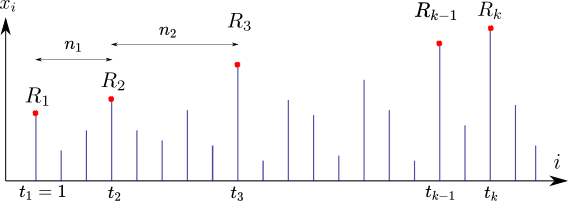
Given this time-series $\{x_{1},\,x_{2},\,x_{3},\cdots\}$ and its underlying probability distribution $P(x_{1},\,x_{2},\,x_{3},\cdots)$, one can investigate various observables associated to the occurrences of records. Three rather natural questions are as follows:

• How many records $M_{N}$ occur in the first $N$ steps? For example, given the joint distribution $P(x_{1},\,x_{2},\,x_{3},\cdots)$, what is the average number of records $\langle M_{N}\rangle$ within the first $N$ steps?

• How are the record values distributed? For example, let

  $$q_{k}(R)={\rm Prob.}[R_{k}=R]$$ (2)

  denote the probability density that the $k$-th record (in the infinite sequence) takes value in $[R,R+dR]$. What can we say about $q_{k}(R)$, given the underlying joint distribution $P(x_{1},\,x_{2},\,x_{3},\cdots)$ of the original entries?

• Suppose that a record occurs at time $t_{k}$. How long does it take to break this record? Let $n_{k}=t_{k+1}-t_{k}$ denote the time gap between the $(k+1)$-th record and the $k$-th record–this is the age of the $k$-th record. Let

  $$\pi_{k}(n)={\rm Prob.}[n_{k}=n]$$ (3)

  denote the distribution of the age of the $k$-th record. Given the joint distribution of entries $P(x_{1},\,x_{2},\,x_{3},\cdots)$, can one compute $\pi_{k}(n)$?

I.I.D model. The simplest model where one can compute exactly all three observables correspond to the case when the entries $x_{i}$’s are uncorrelated and each is drawn independently from a continuous distribution $f(x)$. In other words, the joint distribution factorizes

$$P(x_{1},\,x_{2}\,x_{3},\cdots)=f(x_{1})\,f(x_{2})\,f(x_{3})\cdots$$ (4)

This is usually referred to as the independent and identically distributed (I.I.D) model Chandler52 ; FS54 ; Neuts67 ; Scho72 ; ABN98 ; Nevzorov . The probability density function (PDF) $f(x)$ is normalized to unity and its cumulative distribution is defined as $F(x)=\int_{-\infty}^{x}f(y)\,dy$. We summarize these classical results here, and for a derivation see, e.g., the review GMS17 with citations to the original literature Chandler52 ; FS54 ; Neuts67 ; Scho72 ; ABN98 ; Nevzorov .

(i) It turns out that the average number of records up to first $N$ steps is universal, i.e., independent of $f(x)$ and is given by the simple formula

$$\langle M_{N}\rangle=\sum_{k=1}^{N}\frac{1}{k}\xrightarrow[N\to\infty]{}\ln N\,.$$ (5)

Thus the mean number of records grows very slowly (logarithmically) with increasing $N$ indicating that records get increasingly harder to break. Moreover, the full distribution of $M_{N}$, i.e., $P(M,N)={\rm Prob.}(M_{N}=M)$ is also known and is universal. In the limit $N\to\infty$, the distribution $P(M,N)$ approaches a Gaussian form with mean $\ln N$ and variance $\ln N$.

(ii) The distribution $q_{k}(R)$ of the value of the $k$-th record is also known explicitly

$$q_{k}(R)=f(R)\,\frac{\left[-\ln(1-F(R))\right]^{k-1}}{(k-1)!}\,,\quad k=1,2,\ldots\,.$$ (6)

where $F(R)$ is the cumulative distribution. Unlike the distribution of $M_{N}$, the record value distribution $q_{k}(R)$ is not universal, as it depends explicitly on $f(R)$. For example, for exponentially distributed positive entries with $f(x)=e^{-x}\,\theta(x)$ (where the Heaviside step function $\theta(x)=1$ if $x>0$ and $\theta(x)=0$ if $x\leq 0$), Eq. (6) gives

$$q_{k}(R)=e^{-R}\,\frac{R^{k-1}}{(k-1)!}\,\quad k=1,2\cdots$$ (7)

In this case the average record value $\langle R_{k}\rangle=\int_{0}^{\infty}R\,q_{k}(R)\,dR=k$ increases linearly with $k$. Similarly, the variance of $R_{k}$ also grows linearly with $k$. In fact, for generic $f(x)$ in Eq. (6), one can show that $q_{k}(R)$ does not have a limiting distribution as $k\to\infty$.

(iii) Finally, the age distribution $\pi_{k}(n)$ of the $k$-th record is also known explicitly and turns out to be universal, i.e., independent of $f(x)$. For any $k\geq 1$, it reads GMS17

$$\pi_{k}(n)=\sum_{m=0}^{n-1}\binom{n-1}{m}\frac{(-1)^{m}}{(2+m)^{k}}\underset{n\to\infty}{\simeq}\frac{1}{n^{2}}\,\frac{\left[\ln n\right]^{(k-1)}}{(k-1)!}\,.$$ (8)

Two important points to note for the I.I.D model that will be important in this paper: (a) the distribution $q_{k}(R)$ depends on $k$ even when $k\to\infty$, i.e., there is no limiting stationary record value distribution as $k\to\infty$, simply because the record values grow with $k$ for generic $f(x)$ and (b) similarly, the age distribution $\pi_{k}(n)$ in Eq. (8) also does not have a limiting stationary distribution when $k\to\infty$.

After introducing this basic background, we now turn to the main topic of this paper. Here our goal is to use the tools of record statistics to provide a simple model for the peculiar jerky motion observed in many disordered systems, as a response to an external driving force. In such systems the dynamics of the relevant degree of freedom typically alternates between static immobile states and periods of rapid motion called avalanches. Examples of such a behaviour are quite ubiquitous, ranging from the crack propagation in solids BB11 ; Bonamy17 ; BBR19 , the earthquake of seismic faults AGGL16 or the Barkhausen noise ABBM90 ; ZVS97 ; SDM01 appearing in the magnetisation curve as a function of the applied magnetic field–see FC2008 for a review. Avalanches are well studied in the context of the depinning of an elastic interface pulled through a disordered medium by an external force LDW09 ; ABBM90 ; Kardar98 ; Fisher98 . In the absence of an external force the line is pinned by the disorder. Upon increasing the force beyond a local threshold, a portion of the interface gets depinned and its center of mass moves forward, thus creating an avalanche. Interestingly, a simple one dimensional lattice model for depinning can be mapped exactly to the record model discussed above, as we show below.

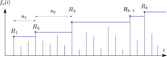
In this lattice model, the elastic line is replaced by a single particle (representing its center of mass) that moves on an infinite $1$-d lattice. Under this mapping, the time series $\{x_{i}\}$ in Fig. (1) gets mapped on to the quenched pinning forces with the horizontal axis $i$ labelling the sites of a $1$-d lattice. This defines the disorder landscape $\{x_{1},x_{2},\dots\}$ on which the particle moves under the effect of the applied force, $f_{a}(i)$ (namely the force applied at the site $i$). The particle leaves the site $i$ if $f_{a}(i)>x_{i}$. Hence, the minimal force profile allowing motion alternate between plateaus and vertical jumps (see Fig.2 ). The plateaus coincide exactly with the record series $\{R_{1},\,R_{2},\,R_{3},\dots\}$ and the vertical jumps occur exactly at the sites $\{t_{1},\,t_{2},\,t_{3}\dots\}$ where the record occurs in Fig.1. The age of the $k$-th record $n_{k}$ in Fig. (1) maps on to the size of the $k$-th avalanche in the depinning model. The three observables $\langle M_{N}\rangle$, $q_{k}(R)$ and $\pi_{k}(n)$ have precise physical meaning in the context of depinning. For example, $\langle M_{N}\rangle$ is the number of jumps of the applied force profile in order to displace the position of the particle by $N$ sites, given that it started at $i=1$. Similarly, $\pi_{k}(n)$ represents the size distribution of the $k$-th avalanche in the depinning model.

In the simple I.I.D setting, the pinning forces $\{x_{i}\}$ in the disordered landscape are independent and identically distributed, each drawn from a continuous PDF $f(x)$. However, as we discuss in detail in Section (II), this simple I.I.D model, while analytically tractable, fails to reproduce the behaviors of the three observables as seen in real systems. In addition, the spatio-temporal correlations in the applied force profile $f_{a}(i)$ (record values) as well as in the avalanches seen in realistic systems are also not reproduced by the I.I.D model. This calls for some amendments in this basic I.I.D model. The idea is to introduce minimal changes in the model such that it retains its analytical tractability, and yet reproduces the features observed in real systems.

After discussing briefly the previous attempts of modifying the simple I.I.D model in Section II, we introduce a new model in this paper which we call the $c$-record model. This model has the I.I.D landscape with input $f(x)$, and one single additional parameter $c>0$ associated with the applied force profile $f_{a}(i)$. The model is precisely defined in Section III. We demonstrate in this paper that the the $c$-record model is (a) exactly solvable with a rich analytical structure and (b) it reproduces qualitatively similar features for all the three observables, as well as the spatio-temporal correlations, that one observes in realistic system of depinning.

Quite remarkably, it turns out that this $c$-record model was already introduced in a different context in the statistics literature by Balakrishnan et. al., where is was called the $\delta$-exceedence record model Bala96 . The parameter $\delta=-c<0$ is negative in our context. In addition, this $\delta$-exceedence model with a negative $\delta=-c<0$ also appeared in the random adaptive walk (RAW) model to describe biological evolution on a random fitness landscape PSNK15 ; PNK16 ; PK16 . In fact, we use the notation $c$ for $-\delta$ in our model following Ref. PSNK15 .

In the context of the RAW model, the two observables $\langle M_{N}\rangle$ and $q_{k}(R)$, but not $\pi_{k}(n)$, were already studied analytically in Ref. PSNK15 . In the notation of Ref. PSNK15 for RAW, our $\langle M_{N}\rangle$ corresponds to the mean walk length of an adaptive walker (for genome size $L$) $D_{\rm RAW}(L)$ in the RAW model, with $L\sim N$ for large $L$. In particular, for exponentially distributed positive fitness landscapes $f(x)=e^{-x}\theta(x)$ where $\theta(x)$ is the Heaviside step function, Ref. PSNK15 uncovered a striking phase transition at the critical value $c=1$, across which the asymptotic growth of $\langle M_{N}\rangle$, with increasing $N$, changes drastically.

In this paper, we re-visit this $c$-record model in the context of depinning and avalanches. We provide a thorough analytical and numerical study of all three observables $\langle M_{N}\rangle$, $q_{k}(R)$ and $\pi_{k}(n)$ and also the underlying correlation structure of the record values and avalanches for a general $f(x)$, including in particular the interesting case $f(x)=e^{-x}\theta(x)$. For this particular case $f(x)=e^{-x}\theta(x)$, while our results fully agree with Ref. PSNK15 for $c\leq 1$, we show that for $c>1$ the model has a much richer structure than was reported in Ref. PSNK15 . In particular, we show that for $c>1$ and $f(x)=e^{-x}\theta(x)$, the average number of records $\langle M_{N}\rangle$ grows for large $N$ as a power law

$$\langle M_{N}\rangle\sim N^{\lambda(c)}\,,$$ (9)

with an exponent $\lambda(c)$ that depends continuously on $c$ (for $c>1$) and is given by the unique positive root of the transcendental equation

$$c=-\frac{\ln(1-\lambda)}{\lambda}\,.$$ (10)

Thus our prediction for the asymptotic growth of $\langle M_{N}\rangle$ in Eq. (9) for $c>1$ differs from Ref. PSNK15 where $\langle M_{N}\rangle\sim O(N)$ was reported. We also show that for $c>1$, the record value distribution $q_{k}(R)$ approaches a stationary distribution as $k\to\infty$, which is given by a pure exponential behaviour for all $R\geq 0$

$$q_{k\to\infty}(R)=\lambda(c)\,e^{-\lambda(c)\,R}\,.$$ (11)

In addition, the avalanche size distribution $\pi_{k}(n)$ also approaches a stationary distribution as $k\to\infty$ (for $c>1$) with a power-law tail

$$\pi_{k\to\infty}(n)\sim n^{-\lambda(c)}\,\quad{\rm as}\quad n\to\infty$$ (12)

where the exponent is the same $\lambda(c)$ as in Eq. (10).

The rest of our paper is organised as follows. In Section II, we recall the mapping between the $1$-d lattice model of depinning and the record model and also discuss previously studied models that go beyond the simple I.I.D record model. In Section III, we define the $c$-record model precisely, and provide a detailed summary of our results. For the particular case $f(x)=e^{-x}\theta(x)$, we also provide a detailed comparison of our results to that of Ref. PSNK15 . In Section IV we set up the exact recursion relations and derive the non-local differential equations for the three main observables, respectively in Subsections IV.1, IV.2, and IV.3. In Section V, we provide the full exact solution of all three observables in the $c$-record model and demonstrate the phase transition at $c=1$. In Section VI we discuss in detail the criterion for stationarity of the record value distribution $q_{k}(R)$ as $k\to\infty$ for a stretched exponential family of $f(x)$. Section VII considers other fanilies of $f(x)$, including an exact solution for the uniform distribution over $[0,1]$ and numerical results for the Weibull class of $f(x)$. In Section VIII we show some possible generalizations of the $c$-record process. Section IX is dedicated to the conclusion. Finally, the derivation of the asymptotic results, rather long and tedious, are relegated to Appendices (A-G).

II Depinning, avalanches and record statistics

To understand how record statistics of a discrete-time series, discussed in the introduction, can be used to study the avalanches associated with the depinning of an elastic interface, we consider a very simple one dimensional model where one replaces the extended interface by a point representing its center of mass LDW09 . The model is defined on an infinite one dimensional lattice where the lattice sites are labelled by $i=1,\,2,\,3,\cdots$. At each site $i$, we assign a positive random variable $x_{i}$, drawn independently from a continuous $f(x)$, representing the local pinning force at site $i$. The time-series $\{x_{i}\}$ in Fig. (1) then defines the quenched random landscape, with the horizontal axis $i$ labelling the lattice sites. The associated record-series $\{R_{1},\,R_{2},\,R_{3},\cdots\}$ in Fig. (1) now defines the record values of this pinning force landscape. We then launch a single particle on this quenched landscape at site $i=1$ and apply an external force $f_{a}$ at site $i=1$ that tries to drag the particle from $i=1$ to the neighbouring site $i=2$. The force $f_{a}$ is increased continuously with time at a constant rate. As long as the value of $f_{a}$ is less than the local pinning force $x_{1}$, the particle does not move from site $1$. Upon increasing the force $f_{a}$, when it just exceeds $x_{1}=R_{1}$, the particle suddenly jumps to site $2$. Let $f_{a}(1)$ denote the applied force just when the particle leaves the site $i=1$. The value of the applied force remains the same, i.e., $f_{a}=f_{a}(1)=x_{1}=R_{1}$ when the particle is moving. When the particle arrives at site $i=2$, if the current force $f_{a}(1)$ is less than $x_{2}$, i.e., $x_{2}$ is a record, the particle gets stuck again at site $2$ and the applied force needs to increase to exceed the pinning force $x_{2}$. However, if $x_{2}$ is not a record, the current force $f_{a}(1)$ is bigger than $x_{2}$ and the particle hops from $i=2$ to $i=3$. Essentially the particle keeps moving forward to the right till it encounters the next record value of the landscape. We then have to increase the force $f_{a}$ to exceed the current record value and the process continues. The number of sites the particle moves forward following a depinning (till it gets pinned again) is precisely the size of an avalanche.

Let $f_{a}(i)$ denote the value of the applied force at site $i$ just when the particle leaves the site $i$. In this simple model, we thus see that the applied force profile $f_{a}(i)$ essentially has a staircase structure alternating between plateaus and vertical jumps (see Fig. (2)). The plateau values of the force $f_{a}(i)$ are precisely the record values $\{R_{1},\,R_{2},\,R_{3},\cdots\}$ of the underlying landscape and the jumps of $f_{a}(i)$ occur exactly at the sites where records occur in the quenched landscape, i.e, they coincide with record-time series $\{t_{1},\,t_{2},\,t_{3}\,\cdots\}$ in Fig. (1). Consequently, the ages $n_{k}$ of the records coincide exactly with the sizes of successive avalanches. Thus the three observables introduced before in Fig. (1) are also very relevant in the context of depinning: (i) $\langle M_{N}\rangle$ measures the average number of jumps the external force has to undergo in order to displace the particle from site $i=1$ to site $i=N$, (ii) $q_{k}(R)$ represents the distribution of the height of the $k$-th plateau of the applied force and (iii) $\pi_{k}(n)$ is precisely the distribution of the size of the $k$-th avalanche.

Figure 2: The applied force profile $f_{a}(i)$ in the $1$-d depinning model has a staircase structure (shown by the solid black line), alternating between plateaus and vertical jumps. The plateau values coincide exactly with the record-series $\{R_{1},\,R_{2},\,R_{3}\,\cdots\}$, while the jumps occur precisely at the sites where the records occur, i.e., at sites $\{t_{1},\,t_{2},\,t_{3},\cdots\}$ of figure (1). The age of the $k$-the record $n_{k}$ coincides exactly with the size of the $k$-th avalanche in the depinning model.

How realistic is this simple depinning model with an I.I.D landscape? It turns out that there are three important features in real systems that the I.I.D model fails to reproduce faithfully:

(1) In real systems, the distribution $q_{k}(R)$ of the height of the $k$-th plateau in the force profile typically approaches a stationary distribution as $k\to\infty$. In contrast, in the I.I.D model, as seen from Eq. (6), there is no limiting stationary distribution for $q_{k}(R)$ as $k\to\infty$.

(2) In real systems, the avalanche size distribution $\pi_{k}(n)$ not only approaches a stationary distribution $\pi(n)$ as $k\to\infty$, but the stationary distribution also has a pure power-law tail, $\pi(n)\sim n^{-\tau}$ as $n\to\infty$ ZVS97 ; BCDS02 ; BDHDB18 (e.g., the celebrated Gutenberg-Richter law for earthquake magnitude). In the I.I.D model, the result in Eq. (8) indicates that $\pi_{k}(n)$ neither approaches a stationary distribution as $k\to\infty$, nor does it have a pure power-law tail.

(3) Real systems exhibit very interesting correlations between the record ages, $n_{k}$, as well as between the record values, $R_{k}$. For example, after a large earthquake occurs, one observes a cascade of large aftershocks followed by long periods of quiescent activity characterized by events of small size. It turns out that in the I.I.D model the record values $R_{k}$’s increase monotonically with $k$ and a similar trend is observed for the ages, leaving no scope for observing cascade of events of large sizes, followed by quiescent activity.

An important improvement over the I.I.D model is represented by the well known Alessandro-Beatrice-Bertotti-Montorsi (ABBM) model introduced to study the avalanches in Barkhausen noise ABBM90 . In the ABBM model, the I.I.D landscape is replaced by a correlated one where $x_{i}$ represents the position of a one dimensional random walk ABBM90 ; FC2008 . In this case, the avalanche size distribution $\pi_{k}(n)$ coincides with the return time distribution of a Brownian motion in $1$-d, and hence $\pi_{k}(n)$ is stationary (independent of $k$) and does have a pure power law tail, $\pi_{k}(n)\sim n^{-\tau}$ with $\tau=3/2$. A similar analysis also follows from the study of record statistics for a random walk sequence MAJ08 . However, in this model, $q_{k}(R)$ does not approach a stationary distribution as $k\to\infty$ (the point (1) above) and the sequence of record ages is uncorrelated at variance with what it is seen in real systems (the point (3) above).

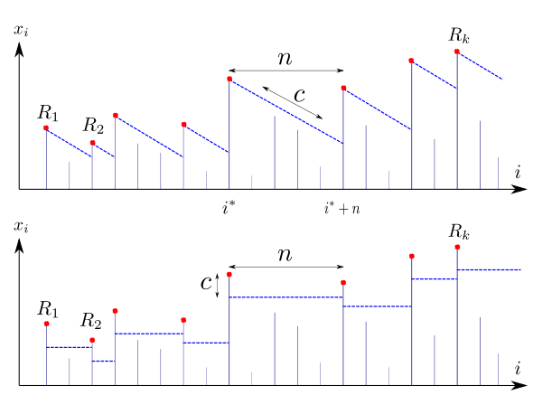
Another modification of the simple I.I.D record model is the so called linear-trend model LDW09 . In this model, the landscape of pinning forces $\{x_{i}\}$ remains I.I.D, but the applied force profile $f_{a}(i)$ changes from Fig. (2) in a simple way (see Fig. (3) upper panel). Just after the particle is deblocked from a pinning site, one assumes that the applied force $f_{a}(i)$ decreases linearly, $f_{a}(i+1)=f_{a}(i)-c$ (with $c>0$) with increasing $i$ till the particle gets blocked again. Thus, as opposed to the horizontal plateaus between two successive records in the I.I.D model (as in Fig. (2)), the force profile in the linear-trend model has a linear behavior with a negative slope, as shown schematically in Fig. (3) upper panel. The physical rationale behind the decrease of the applied force is the dissipation during the avalanche motion (in particular we have a linear decrease if $f_{a}(i)$ is the elastic force between the particle and a drive that moves at a constant slow rate). In this model, at the end of an avalanche when the particle gets stuck at a new site, the force profile $f_{a}(i)$ jumps again to the corresponding record value of the landscape at that site and the process continues. The sequence of the force values at the beigining of an avalanche coincides with the record series $\{R_{1},\,R_{2},\,R_{3},\,\cdots\}$ of the landscape (see Fig. (3) upper panel).

Interestingly, it turns out that this linear-trend model was also introduced originally in the statistics literature by Ballerini and Resnick BR85 ; BR87 , and has since been studied extensively with numerous applications B99 ; FWK10 ; WFK11 ; FWK12 . The analysis of the linear-trend model with $c>0$ shows that the average number of records grows linearly with $N$ for large $N$, i.e., $\langle M_{N}\rangle\approx a(c)\,N$ where the prefactor $a(c)$ is nontrivial and nonuniversal, i.e., depends on $f(x)$ BR85 ; FWK10 ; WFK11 . The record value distribution $q_{k}(R)$ (or equivalently the distribution of the applied forces at the begining of the $k$-th avalanche) does approach a stationary distribution as $k\to\infty$ (as in realistic systems) that depends on the tail of $f(x)$. Similarly, the avalanche size distribution $\pi_{k}(n)$ also approaches a stationary distribution $\pi(n)$ as $k\to\infty$, however this stationary distribution $\pi(n)$ does not have a power-law tail (rather an exponential cut-off) for large $n$ as expected in real systems. In summary, the linear-trend model does reproduce some features of avalanches in realistic depinning systems, but not all.

In this paper, we introduce a simple modification of the linear-trend model, which we call the $c$-record model. The model is defined more precisely in the next section where we also provide a summary of our main results. This model allows exact solutions for the three observables $\langle M_{N}\rangle$, $q_{k}(R)$ and $\pi_{k}(n)$. We show that these observables as well as the correlation structure between records and their ages reproduce the features observed in realistic systems.

Figure 3: Schemes for modified records. Upper panel: linear trend records. Lower panel: $c$-records.

III $c$-record model: the definition and a summary of main results

The model. The $c$-record model that we study in this paper is defined as follows. Once again, we consider an infinite I.I.D landscape $\{x_{1},\,x_{2},\,x_{3},\cdots\}$ of quenched pinning forces defined on a $1$-d lattice, where each entry is chosen independently from a continuous PDF $f(x)$. Let $\{R_{1},\,R_{2},\,R_{3},\cdots\}$ denote the record-series of this landscape. As in the simple I.I.D model, the particle starts from site $i=1$ and it can leave the this site when the local applied force $f_{a}$ exceeds the pinnning force $x_{1}$. The only difference in our model from that of the linear-trend model discussed in the previous section, is how the force profile $f_{a}(i)$ behaves between two avalanches. In the linear-trend model, the force profile following a record decreases linearly till the next record (as in Fig. (3) upper panel). In contrast, in the $c$-record model, we assume that following a record, the force decreases by $c$ only in the first step, but after that it stays flat till it encounters the next record (see Fig. (3) lower panel). More precisely, between two successive record values $R_{k}$ at $t_{k}$ and $R_{k+1}$ at $t_{k+1}$ we now have

$$f_{a}(i)=R_{k}-c,\,{\rm for}\,\,i=t_{k}+1,t_{k}+2,\cdots,t_{k+1}-1\,.$$ (13)

At $i=t_{k+1}$, the force $f_{a}(i)$ undergoes a jump to the associated record value $R_{k+1}$ of the landscape. The physical rationale behind this new model is that the dissipation in the force profile that occurs just after depinning is short-ranged in time, e.g., occurs only during the first hopping but stays constant afterwards.

The formation of records in this $c$-record depinning model can be alternatively phrased in the language of standard time-series discussed in the introduction. Consider, as before, an infinite I.I.D sequence of entries $\{x_{1},\,x_{2},\,x_{3}\,\ldots\}$ each drawn from $f(x)$. Here a record series $\{R_{1},\,R_{2},\,R_{3},\ldots\}$ is formed recursively, in the presence of a single parameter $c>0$, as follows. If a record occurs at some step with record value $R$, a subsequent entry will be a record only if its value exceeds $(R-c)\,\theta(R-c)$. Clearly, for $c=0$, this is the standard record model discussed in the introduction. For $c>0$, this is precisely the $\delta$-exceedence model introduced by Balakrishnan et. al. Bala96 with $\delta=-c<0$. As already discussed in the introduction, this model with $c>0$ was also studied in Ref. PSNK15 as the random adaptive walk (RAW) model of biological evolution in a random fitness landscape.

In this paper, we have studied the three observables $\langle M_{N}\rangle$, $q_{k}(R)$ and $\pi_{k}(n)$ in the $c$-record model, both analytically and numerically, for a class of $f(x)$’s. From the motivation of the depinning pheomenon, our main interest is to determine if, when $k\to\infty$, the $c$-record process becomes ‘stationary’ or not. We say that it is stationary if the distributions $q_{k}(R)$ and $\pi_{k}(n)$ have a well defined limit as $k\to\infty$, namely:

$$\lim_{k\to\infty}q_{k}(R)=q(R)$$ (14)

$$\lim_{k\to\infty}\pi_{k}(n)=\pi(n)$$

Below we summarize our main results.

The summary of main results. We find that for $c>0$, the behavior of all three observables depend explicitly on $f(x)$ and $c$. For simplicity, we consider positive random variables, i.e., $f(x)$ with a positive support. In particular, three cases can be distinguished:

1. If $f(x)$ decays slower than any exponential function as $x\to\infty$, then the record process doesn’t reach a stationary limit for any $c>0$, i.e., $q_{k}(R)$ and $\pi_{k}(n)$ do not have a $k$-independent limiting distribution as $k\to\infty$. The average number of records $\langle M_{N}\rangle$ grows logarithmically with $N$ as in the standard record problem $c=0$ (but with a different subleading constant):

   $$\langle M\rangle_{N}=\ln N+O(1)$$ (15)

2. If $f(x)$ decays faster than any exponential function as $x\to\infty$ (this includes bounded distribution), then the average number of records grows linearly with $N$ at the leading order:

   $$\langle M\rangle_{N}=A_{1}(c)N+O(N)$$ (16)

   where the amptitude $A_{1}(c)$ can be analytically determined in some cases, e.g., for uniform $f(x)$ over the interval $[0,1]$ (see Eq. (72)). In this case, the record process also reaches a stationary limit for all $c>0$. We compute the stationary record value distribution $q(R)$ and the stationary age distribution $\pi(n)$, analytically and numerically, in several examples of $f(R)$. In particular, for distributions with a finite support, we show that $\pi(n)$ decays exponentially with $n$ for large $n$. Finally, for distributions with unbounded support and $f(x)\to e^{-x^{\gamma}}$ as $x\to\infty$ with $\gamma>1$, we show that $\pi(n)$ still has a power-law tail with an exponent larger than $2$.

The case $f(x)=\exp(-x)$ that separates these two behaviors turns out to be marginal, with a striking phase transition at $c=1$. While for $0\leq c\leq 1$, there is no limiting stationary distribution for $q_{k}(R)$ and $\pi_{k}(n)$ as $k\to\infty$, we show that for $c>1$, they do approach stationary distributions. In particular, we find that for $c>1$

$$q(R)=\lambda(c)e^{-\lambda(c)\,R}$$ (17)

$$\pi(n\to\infty)=\frac{\lambda(c)(1-\lambda(c))}{n^{1+\lambda(c)}}$$ (18)

where $\lambda(c)$ is the unique positive root of the transcendental equation:

$$c=-\frac{\ln(1-\lambda)}{\lambda}$$ (19)

The average number of records $\langle M_{N}\rangle$ is computed exactly in Eq. (36) and its large $N$ behavior also exhibits a phase transition at $c=1$. we show that

$$\langle M\rangle_{N}=\begin{cases}\frac{1}{1-c}\ln N-\mu(c)+O(\frac{1}{N})&0\leq c<1\\ \\ \ln^{2}N+O(\ln N)&c=1\\ \\ A_{0}(c)N^{\lambda(c)}+\frac{1}{1-c}\ln N+O(1)&c>1\end{cases}$$ (20)

where the exponent $\lambda(c)$ depends continuously on $c$ and is given in Eq. (19). Note that $\lambda(c)$ increases monotonically with increasing $c\geq 1$: $\lambda(c)\to 0$ as $c\to 1^{+}$, while $\lambda(c)\to 1$ only when $c\to\infty$. The explicit expression of the constant $A_{0}(c)$ is given in equation (117). The constant $\mu(c)$ can be evaluated using the method explained in appendix (B). We also provide careful numerical checks for all our analytical formulae.

As mentioned in the introduction, precisely this marginal case $f(x)=e^{-x}$ was also studied in Ref. PSNK15 in the context of RAW model in evolutionary biology and indeed, this striking phase transition at $c=1$ was already noticed there. In Ref. PSNK15 , two of the three observables namely $\langle M_{N}\rangle$ and $q_{k}(R)$ (but not $\pi_{k}(n)$) were studied in detail, but using different notations, language and method. In order to compare our results to those of Ref. PSNK15 , it is useful to provide a dictionary of notations for the reader. In the limit of large genome size $L$, the RAW model studied in PSNK15 becomes equivalent, in the ensemble sense, to our $c$-record model with $N\sim L$. In this limit, our average number of records $\langle M_{N}\rangle$ for large $N$ then translates to the mean length of the adaptive walk $D_{\rm RAW}(L\sim N)$ in PSNK15 for large $L$. Furthermore, our record value distribution $q_{k}(R)$ is precisely $Q_{l=k}(y=R,L\to\infty)$, the probability for the adaptive walker to take $l=k$ steps to arrive at a local fitness $c(l-L)+y$ in the limit of large genome size $L\to\infty$. Hence, to summarize, for large $L$ (or equivalently for large $N$ in our notation)

$$N\sim L\,;\quad\langle M_{N}\rangle\equiv D_{\rm RAW}(L\sim N)\,;$$

$$q_{k}(R)\equiv Q_{l=k}(y=R,L\to\infty)\,.$$ (21)

With the precise translation in Eq. (21) we can now compare our results with those of Ref. PSNK15 . We start with the asymptotic large $N$ behavior of the average number of records $\langle M_{N}\rangle$. For $c\leq 1$, our leading order large $N$ results for $\langle M_{N}\rangle$ in Eq. (20) agree with that of Ref. PSNK15 , though the subleading constant $-\mu(c)$ for $0\leq c<1$ was not computed in PSNK15 . However, for $c>1$, our result in Eq. (20) is much richer (characterized by a power law growth of $\langle M_{N}\rangle$ with an exponent depending continuously on the parameter $c$) and different from that of PSNK15 where $\langle M_{N}\rangle\sim O(N)$ was reported (see Eq. (15) of PSNK15 ). We find that the growth of $\langle M_{N}\rangle$ with increasing $N$ becomes linear only when $c\to 1$, since only in that limit $\lambda(c)\to 1$ in Eq. (20).

Next we turn to $q_{k}(R)$ for $c>1$. In this case, an exact summation formula for $q_{k}(R)$ was derived for all $c$ in PSNK15 (see their Eq. (8)). In the limit $k\to\infty$, this sum is convergent only for $c>1$. In Ref. PSNK15 , this sum was not analysed in the limit $k\to\infty$, since they didn’t need it in their problem. In fact, it can be checked that their Eq. (8), in the limit $k\to\infty$ and for $c>1$, satisfies the fixed point differential equation, $q^{\prime}(R)=q(R+c)-q(R)$ (see later in Eq. (42)), whose solution is precisely a single pure exponential $q(R)=\lambda(c)\,e^{-\lambda(c)\,R}$, with $\lambda(c)$ given by the positive root of Eq. (19). This is a rather nontrivial confirmation that two different methods lead to the same solution.

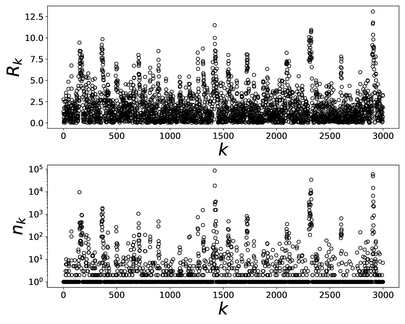
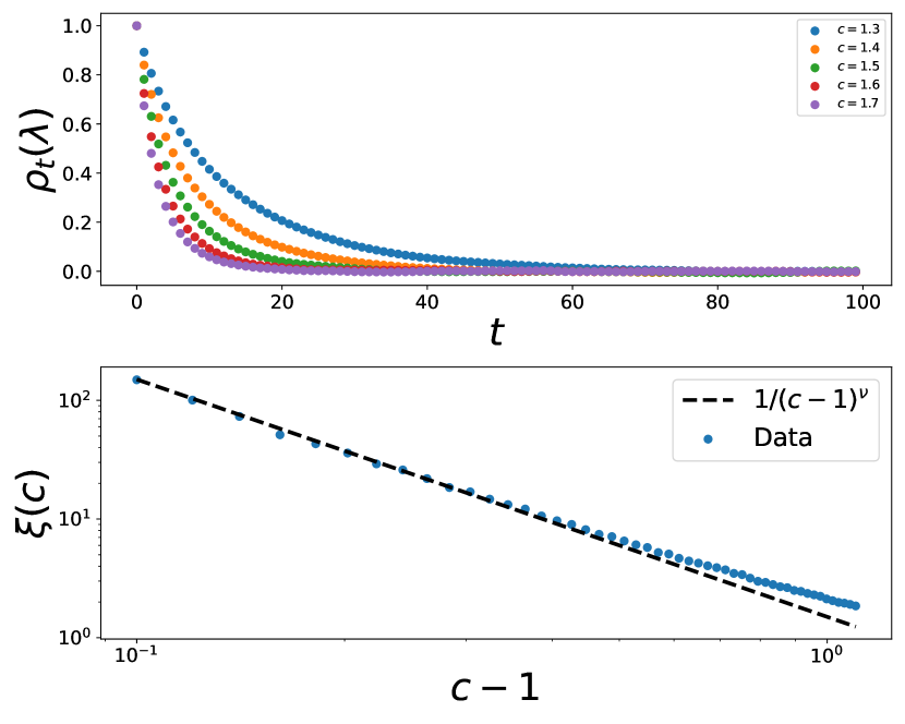
Let us finally conclude this summary section by mentioning that we have also studied the correlations between record values in the stationary state when it exists. In that case, the sequence of records display remarkable clustering properties (see Fig. 4 upper panel)): after a large record value, we observe other large record values followed by a swarm of smaller record values. In the exponential case $f(x)=e^{-x}$, we show that the correlation between record values $\langle R_{k}R_{k+\tau}\rangle$ decreases exponentially with increasing $\tau$. The value of $c$ controls the correlation length: when $c\to 1$ from above, the correlation lengths diverges as $\sim 1/(c-1)^{2}$ reminiscent of the critical phenomena (see Fig. 8)). We also study the clustering property of record ages that correspond to avalanches (see Fig. 4 lower panel)). This property is qualitatively similar to what is observed in seismic catalogs.

Figure 4: Typical sequence of $c$-record values (upper panel) and their ages (lower panel) computed from a series of exponential number and using $c=1.5$. Note that large record values and large ages are organized in well defined clusters.

IV Setting up the recursion relations for the three observables

In this section, we show how to set up the basic recursion relations to compute the three observables in the $c$-record model: (i) the mean number of records $\langle M_{N}\rangle$ up to $N$ steps, (ii) the distribution $q_{k}(R)$ of the value of the $k$-th record and (iii) the distribution $\pi_{k}(n)$ of the time interval $n_{k}$ between the $k$-th and the $(k+1)$-th record. For simplicity, we will assume throughout that we have an infinite series of I.I.D entries $\{x_{1},\,x_{2},\,x_{3},\,\cdots\}$, each drawn from a continuous $f(x)$ which has a positive support, i.e., the entries are non-negative random variables.

IV.1 The Number of Records

In this subsection we derive the exact recursion relation that we have used to compute $\langle M\rangle_{N}$. It turns out that the main object that we need for this computation is the joint probability density $P_{N}(M,R_{M}=R)$ that in the first block of size $N$ of the infinite series of random entries there are exactly $M$ records and that the last record has value $R$. This quantity $P_{N}(M,R)$ satisfies a closed recursion relation

$$P_{N}(M,R)=P_{N-1}(M,R)\theta(R-c)\int_{0}^{R-c}f(x)dx+\\ +f(R)\int_{0}^{R+c}P_{N-1}(M-1,R^{\prime})dR^{\prime}$$ (22)

with $\theta(x)$ the Heaviside step function. It is straightforward to understand Eq. (22): the first term on the right hand side (r.h.s) accounts for the event when the $N$-th entry is not a record, while the second term corresponds to the event when the $N$-th entry is a record. In the first case, given that the last record has value $R$, the value of the $N$-th entry $x_{N}$ must be less than $R-c$ which happens with probability $\int_{0}^{R-c}f(x)dx$. In the second case, the $N$-th entry is a record with value $R$, hence the previous record $R^{\prime}$ must be less than $(R+c)$ explaining the second term on the r.h.s in Eq. (22). The recursion relation (22) starts from the initial condition

$$P_{1}(M,R)=\delta_{M,1}\,f(R)\,,$$ (23)

since the first entry, by convention, is a record. The recursion relation (22), starting from (23), is nontrivial to solve since it relates $P_{N}(M,R)$ at $R$ to its integral up to $R+c$ at step $N-1$, making it a non-local integral equation for any $c>0$.

In order to compute $\langle M\rangle_{N}$, namely the average number of records as a function of $N$, we introduce $\tilde{Q}(R,z,s)$ as the double generating function of $P_{N}(M,R)$:

$$\tilde{Q}(R,z,s)=\sum_{N=1}^{\infty}\sum_{M=1}^{\infty}P_{N}(M,R)z^{N}s^{M}$$ (24)

Using equation (22) with the initial condition (23), we obtain the following equation for (24):

$$\tilde{Q}(R)\left[1-zF(R-c)\theta(R-c)\right]=\\ zsf(R)\left[1+\int_{0}^{R+c}\tilde{Q}(R^{\prime})dR^{\prime}\right]$$ (25)

For simplicity, we omitted the arguments $z$ and $s$ of $\tilde{Q}$. Evidently, Eq. (25) is also non-local with respect to $R$ for any $c>0$.

Even though the full joint distribution $P_{N}(M,R)$ of the number of records $M$ and the last record value $R$ is of interest as it contains several interesting informations, we will focus on the simplest quantity, namely the mean number of records $\langle M\rangle_{N}$. To compute this, we need to extract $P_{N}(M)$, the distribution of the number of records $M$ up to $N$ steps. This is obtained by integrating over the value $R$ of the last record up to $N$ steps

$$P_{N}(M)=\int_{0}^{\infty}P_{N}(M,R)dR\,.$$ (26)

The double generating function of $P_{N}(M)$ is then related to $\tilde{Q}(R,s,z)$ simply by

$$\sum_{N=1}^{\infty}\sum_{M=1}^{\infty}P_{N}(M)z^{N}s^{M}=\int_{0}^{\infty}\tilde{Q}(R,z,s)dR\,$$ (27)

where $\tilde{Q}(R,z,s)$ is the solution of the integral equation (25). Using Eq. (27), the average number of records can be obtained from the relation

$$\langle M\rangle_{N} = \sum_{M=1}^{\infty}M\,P_{N}(M)$$ (28)

$$= \frac{1}{N!}\,\partial^{N}_{z}\partial_{s}\int_{0}^{\infty}\tilde{Q}(R,z,s)dR\,|_{z=0,s=1}\,.$$

Solving the recursion relation (25) for arbitrary $f(x)$ seems hard. However, we were able to compute $\tilde{Q}$ and from it $\langle M_{N}\rangle$ explicitly for two special cases: the exponential distribution $f(x)=e^{-x}\,\theta(x)$ and the uniform distribution $f(x)=\mathbb{I}_{[0,1]}(x)$ with $\mathbb{I}_{[a,b]}(x)$ denoting the indicator function which is $1$ if $x$ belongs to the interval $[a,b]$ and zero otherwise.

IV.2 The record value distribution

In this subsection we derive an exact recursion relation for the $k$-th record value distribution $q_{k}(R)$ in the $c$-record model. We start from the joint conditional probability $q(R,n|R^{\prime})$ that, given a record with value $R^{\prime}$ has occurred at some instant in the infinite sequence, the next record has value $R$ and the age of the current record with value $R^{\prime}$ is $n$, i.e, there are $n$ steps separating the current record and the next record. This conditional probability can be very simply computed

$$q(R,n|R^{\prime})=\begin{cases}f(R)\,\delta_{n,1}\,&R^{\prime}<c\\ &\\ f(R)\,\left[F(R^{\prime}-c)\right]^{n-1}\,\theta(R-R^{\prime}+c)\,&R^{\prime}>c\end{cases}$$ (29)

where we recall that $F(R)=\int_{0}^{R}f(y)\,dy$ is the cumulative distribution of each entry of the underlying time-series. Eq. (29) is easy to interpret: when the previous record $R^{\prime}$ is smaller than $c$, the very next entry with any positive value $R>0$ will be a record, indicating that $n=1$ is the only possible value. In contrast, when $R^{\prime}>c$, assuming that there are exactly $n-1$ entries separating two successive records with values $R^{\prime}$ and $R$ (with $R>R^{\prime}-c$), each of these intermediate entries must be less that $R^{\prime}-c$ (in order that none of them is a record), explaining the factor $\left[F(R^{\prime}-c)\right]^{n-1}$. The probability that the $n$-th entry is a record is simply $f(R)\,\theta(R-R^{\prime}+c)$. By summing over all possible age values $n\geq 1$ we obtain the distribution of the next record value conditioned on the previous one:

$$q(R|R^{\prime}) = \sum_{n=1}^{\infty}q(R,n|R^{\prime})=f(R)\,\theta(c-R^{\prime})$$

$$+ \frac{f(R)}{1-F(R^{\prime}-c)}\,\theta(R-R^{\prime}+c)\,\theta(R^{\prime}-c)$$

Equations (29) and (IV.2) are particularly useful when simulating directly the $c$-record process (see appendix G).

A recursion relation for $q_{k}(R)$ can then be set up using this conditional probbaility $q(R|R^{\prime})$ as

$$q_{k+1}(R) = \int_{0}^{\infty}q_{k}(R^{\prime})\,q(R|R^{\prime})\,dR^{\prime}=f(R)\int_{0}^{c}q_{k}(R^{\prime})dR^{\prime}$$

$$+ f(R)\int_{c}^{R+c}\frac{q_{k}(R^{\prime})}{1-F(R^{\prime}-c)}dR^{\prime}\,,$$

with the initial condition $q_{1}(R)=f(R)$. This relation can be easily understood as follows. The first term takes into account the event when the record $R^{\prime}$ is in the range $0\leq R^{\prime}\leq c$. In this case, the entry immediately after this record is a record with probability $f(R)$. The second term on the r.h.s in Eq. (IV.2) accounts for the contributions coming from the case when $c\leq R^{\prime}\leq R+c$. In this case, one needs to use $q(R|R^{\prime})$ from Eq. (IV.2) and integrate over all allowed values of $R^{\prime}$. This relation (IV.2) was also derived in PSNK15 using different notations and for different observables, in the context of the RAW model of evolutionary biology. Furthermore, for $c=0$, this relation was used in Ref. RP06 for studying the global temperature records.

When the stationary limit of $q_{k}(R)$ exists, $q(R)=\lim_{k\to\infty}q_{k}(R)$ has to satisfy the following fixed point equation

$$q(R) = f(R)\,\int_{0}^{c}q(R^{\prime})dR^{\prime}$$ (32)

$$+ f(R)\,\int_{c}^{R+c}\frac{q(R^{\prime})}{1-F(R^{\prime}-c)}\,dR^{\prime}\,.$$

This is also a non-local differential equation for any $c>0$ and is hard to solve for general $f(x)$. Again, we will see later that for $f(x)=e^{-x}\theta(x)$ (with $c>1$) and for the uniform distribution, it is possible to obtain explicitly the fixed point stationary solution of Eq. (32).

IV.3 The age distribution of records

In this subsection, we derive a recursion relation for $\pi_{k}(n)={\rm Prob.}(n_{k}=n)$ denoting the distribution of the age $n_{k}$ of the $k$-th record, in an infinite I.I.D series. The distribution $\pi_{k}(n)$ can be obtained from the previously defined conditional probability $q(R,n|R^{\prime})$ (29) and the record value distribution $q_{k}(R)$ as follows.

$$\pi_{k}(n) = \int_{0}^{\infty}\int_{0}^{\infty}q(R,n|R^{\prime})\,q_{k}(R^{\prime})\,dR\,dR^{\prime}$$

$$= \delta_{n,1}\,\int_{0}^{c}q_{k}(R^{\prime})\,dR^{\prime}$$

$$+ \int_{c}^{\infty}(1-F(R^{\prime}-c))F^{n-1}(R^{\prime}-c)q_{k}(R^{\prime})dR^{\prime}$$

where we used $F(R^{\prime}-c)=0$ if $R^{\prime}-c\leq 0$. The stationary distribution $\pi(n)$, when it exists, is obtained by taking the limit $\lim_{k\to\infty}\pi_{k}(n)$ and using $q(R)=\lim_{k\to\infty}q_{k}(R)$:

$$\pi(n) = \delta_{n,1}\,\int_{0}^{c}q(R^{\prime})\,dR^{\prime}$$

$$+ \int_{c}^{\infty}(1-F(R^{\prime}-c))F^{n-1}(R^{\prime}-c)\,q(R^{\prime})\,dR^{\prime}\,.$$

Thus, knowing the fixed point distribution $q(R)$ of the record value when it exists, one can compute the stationary age distribution using Eq. (IV.3). Later, we will compute $\pi(n)$ explicitly for the two solvable cases, namely the exponential distribution $f(x)=e^{-x}\theta(x)$ with $c>1$ and the case of the uniform distribution over $[0,1]$.

V Exponential case

In this section we study in detail the exponential case with $f(x)=\exp(-x)\,\theta(x)$.

V.1 Number of records

For the exponential distribution equation (25) reduces to:

$$\tilde{Q}(R)\left[1-z(1-e^{-(R-c)})\theta(R-c)\right]=\\ z\,s\,e^{-R}\,\left[1+\int_{0}^{R+c}\tilde{Q}(R^{\prime})dR^{\prime}\right]$$ (35)

The non-locality manifest in Eq. (25) makes it hard to find its general solution. Remarkably, for the exponential $f(x)$, this is possible. Performing a rather involved calculation, reported in appendix (A), we computed the generating function for $P_{N}(M)$ defined in Eq. (27). Its explicit form is given in Eq. (93) from which we extracted the average number of records $\langle M\rangle_{N}$, obtaining

$$\langle M\rangle_{N}=N!\sum_{m=0}^{N-1}(-1)^{m}\frac{\prod_{k=1}^{m}(k-1+e^{-kc})}{(m+1)!^{2}(N-m-1)!}$$ (36)

This result for $\langle M_{N}\rangle$ is exact for all $N\geq 1$. For example, the first few values of $N$ yield

$$\langle M\rangle_{1}=1$$ (37)

$$\langle M\rangle_{2}=2\left(1-\frac{1}{4}e^{-c}\right)$$ (38)

$$\langle M\rangle_{3}=3\left[1-\frac{4}{9}e^{-c}+\frac{1}{18}e^{-3c}\right]$$ (39)

A non trivial check of equation (36) is for $c=0$. By plugging $c=0$ the term $\prod_{k=1}^{m}(k-1+e^{-kc})$ simplifies to $k!$. Thus equation (36) becomes:

$$\langle M\rangle_{N}=\sum_{m=0}^{N-1}\binom{N}{m+1}(-1)^{m}\frac{1}{(m+1)}$$ (40)

The above expression can be shown to coincide with the well known result $\langle M\rangle=1+1/2+1/3+\dots+1/N$. This can be done by considering the difference $\langle M\rangle_{N}-\langle M\rangle_{N-1}$. While the exact formula (36) is useful to compute the result for moderate values of $N$, the asymptotic behavior of $\langle M\rangle_{N}$ for large $N$ is difficult to extract from it.

Indeed, to extract the large $N$ behvaior, we use a different approach reported in appendix (B) which leads to our main result in Eq. (20) and shows the existence of a phase transition at $c=1$. The presence of the phase transition at $c=1$ in the asymptotic behavior of $\langle M_{N}\rangle$ in Eq. (20) is also related to the fact that both $q_{k}(R)$ and $\pi_{k}(n)$ has stationary limiting distributions as $k\to\infty$, only for $c>1$ as shown in the next subsection V.2. To check the validity of our analytical prediction we also performed direct numerical simulations using $N=10^{6}$ random variables and averaging over $10^{4}$ realizations. The results are shown in Fig. (5) for $c=1.5$ and in Fig. (6) for $c=0.5$, as well as for the marginal case $c=1$.

Figure 5: Exponential case: mean number of $c$-records for $c=1.5$. Blue symbols correspond to numerical data. Black dashed line corresponds to the analytical prediction $A_{0}(c)N^{\lambda(c)}$. The values of the constants are $A_{0}(1.5)=3.4376$, $\lambda(1.5)=0.5828$ (obtained from equations (19) and (117) using Mathematica). Inset: the subleading behavior $\langle\Delta M\rangle_{N}=A_{0}(c)N^{\lambda(c)}-\langle M\rangle_{N}$. Black dashed line corresponds to $-\frac{1}{1-c}\ln N$.

Figure 6: Exponential case: mean number of $c$-records for $c=0.5$ (red circles) and for $c=1$ (orange circles). Circles are numerical data. Black dashed lines correspond to the analytical predictions of Eq.(20). For $c=0.5$ we find $\mu(c)=1.42878\ldots$ computed using Mathematica by the method of appendix (B).

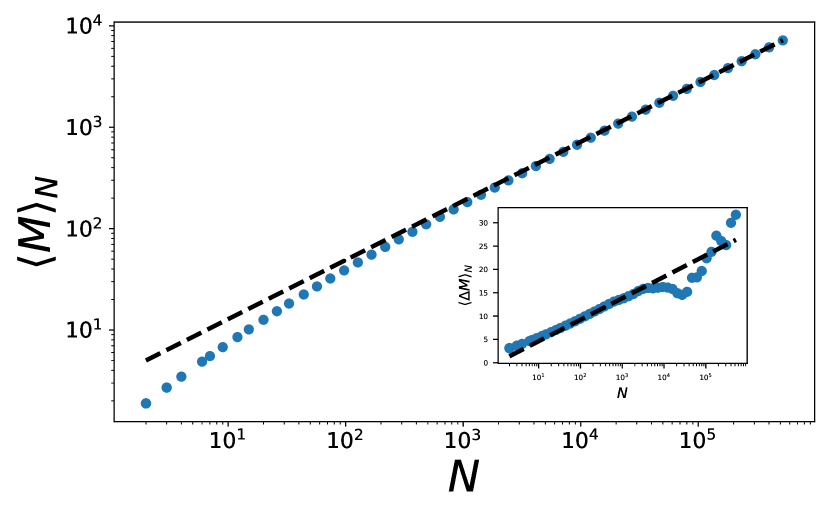
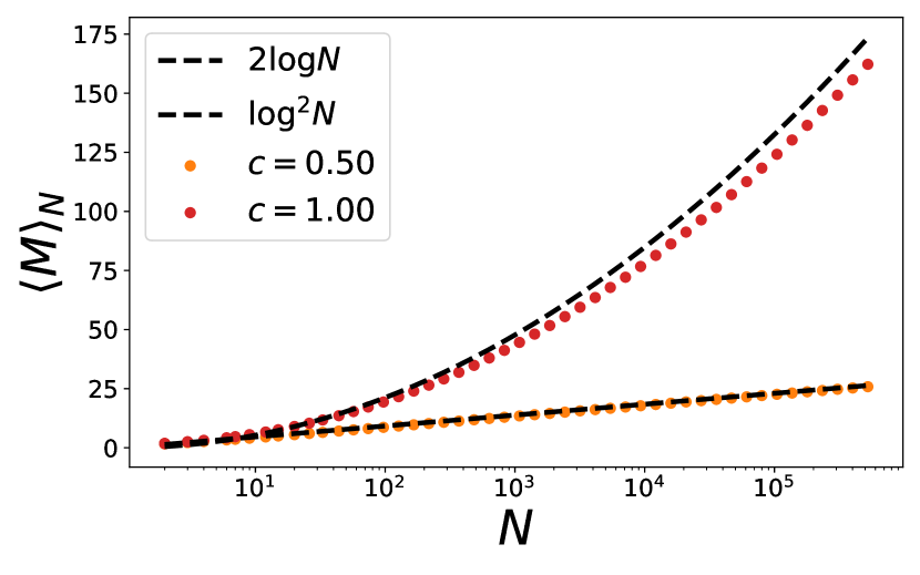
V.2 Stationary record and age statistics

The solution of Eq. (IV.2) for a given $k$ has been studied by Park et al. in PSNK15 for the case $f(x)=\exp(-x)\,\theta(x)$. Here we focus instead on the stationary limit and we seek the solution of Eq. (32). By taking a derivative with respect to (w.r.t.) $R$ of equation (32) we get

$$q^{\prime}(R)=\frac{f(R)}{1-F(R)}q(R+c)+\frac{f^{\prime}(R)}{f(R)}q(R)$$ (41)

For the exponential case, using $f(R)=\exp(-R)$ and $1-F(R)=\exp(-R)$, equation (41) reduces to:

$$q^{\prime}(R)=q(R+c)-q(R)$$ (42)

To solve this equation we use the ansatz:

$$q(R)=\lambda\,e^{-\lambda R}$$ (43)

Equation (42) becomes

$$1-\lambda=e^{-\lambda c}$$ (44)

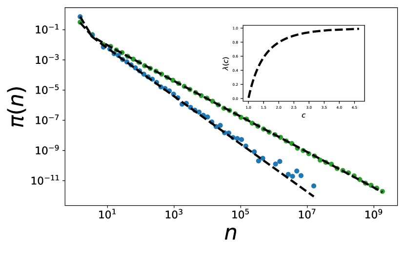
A positive solution for $\lambda=\lambda(c)$ exists only for $c>1$. This means that for $c\leq 1$ there is no stationary regime. This conclusion was already pointed out in PSNK15 based on scaling arguments and numerical simulations. Here we perform an explicit calculation which is also confirmed by the independent calculation of the large $N$ expansion of $\langle M\rangle_{N}$ report in the appendix (B). The stationary average record value is $1/\lambda(c)$ (see inset of Fig. (7)) and has the following limiting behaviors:

$$\langle R\rangle(c)=1/\lambda(c)=\begin{cases}1/2(c-1)&c\to 1^{+}\\ 1&c\to\infty\end{cases}$$ (45)

The divergence as $c\to 1^{+}$ is one of the fingerprints of the absence of a stationary state for $c\leq 1$.

We now turn to the age distribution $\pi_{k}(n)$. As in the case of $q_{k}(R)$, a stationary distribution $\pi(n)$ in the limit $k\to\infty$ exists only for $c>1$. For $c\leq 1$, $\pi_{k}(n)$ depends explicitly on $k$ even in the $k\to\infty$ limit. To derive the stationary age distribution $\pi(n)$ for $c>1$, we substitute $q(R)$ from Eq. (43) into Eq. (IV.3). Upon carrying out the integration explicitly, we obtain the following exact expression of $\pi(n)$ in the stationary state valid for all $n\geq 1$ and $c>1$

$$\pi(n)=\lambda\delta_{n,1}+(1-\lambda)\frac{\lambda\Gamma(n)\Gamma(\lambda+1)}{\Gamma(n+\lambda+1)}\,,$$ (46)

where $\Gamma(z)=\int_{0}^{\infty}e^{-x}\,x^{z-1}\,dx$ is the standard Gamma function. The stationary age (or avalanche size) distribution $\pi(n)$ is then the sum of two contributions: a delta peak at $n=1$ and the Yule-Simon form for $n\geq 1$. Using the asymptotic behavior, $\Gamma(n)\Gamma(\alpha)/\Gamma(n+\alpha)\to 1/n^{\alpha}$ for large $n$, we unveil a beautiful power law behavior of the stationary age distribution (see Fig. (7))

$$\pi(n\to\infty)=\frac{\lambda(1-\lambda)}{n^{1+\lambda}}$$ (47)

where $\lambda\equiv\lambda(c)$ is given by the positive root of Eq. (44) for $c>1$. Note that the power law exponent $(1+\lambda(c))$ continuously varies with $c$. When $c\to\infty$, the exponent $\lambda(c)\to 1$, thus strengthening the amplitude of the delta peak and in addition, for large $n$, the power law tail behaves as $\pi(n)\sim 1/n^{2}$.

We now show that the power law decay of $\pi(n)\sim n^{-(1+\lambda(c))}$ for large $n$ in Eq. (47) for $c>1$ is completely consistent with the result $\langle M_{N}\rangle\sim N^{\lambda(c)}$ for large $N$ in the third line of Eq. (20). To see this, we use a simple scaling argument. Given $\pi(n)\sim n^{-(1+\lambda(c))}$ for large $n$ and the length of the series $N$, the mean inter-record distance (mean age of a record) scales, for large $N$, as

$$\langle n\rangle=\sum_{n=1}^{N}n\,\pi(n)\sim N^{1-\lambda(c)}\,.$$ (48)

Consequently, the mean number of records, which is identical to the mean number of inter-record intervals, up to step $N$ scales for large $N$ as

$$\langle M_{N}\rangle\sim\frac{N}{\langle n\rangle}\sim N^{\lambda(c)}\,,$$ (49)

which reproduces the third line of Eq. (20) for $c>1$. In appendix (A), this result is proved more rigorously.

Figure 7: Exponential case: age statistics of the stationary $c$-records process for $c=1.5$ (blue circles) and for $c=1.1$ (green circles). Numerical data are averaged over $10^{4}$ realizations. Black dashed line corresponds to the analytical predictions of Eq.(46). The inset shows $\lambda(c)$ as a function of $c$.

Figure 8: Upper panel: record correlation function numerically computed as in equation (50). Lower panel: correlation length $\xi(c)$ as a function of $c-1$. We fitted an exponent $\nu\approx 2$.

V.3 Record correlations

One of the most interesting features of the $c$-records statistics is shown in Fig. (4). We focus on a sequence of records when the stationary regime is already reached. The sequence tends to cluster in patterns where record values are high, followed by events of smaller value. The corresponding sequence of ages shows a similar behavior: when the record values are high we observe large ages, while the age is of the order $1$ when the records are small.
To understand this behavior we can first observe that in the classical record case $c=0$, even if there is no stationary regime, all the records values are strongly correlated. As a fingerprint of this, the sequence of record values is strictly increasing. For $c>0$ this is not always the case. For example we know that the $c$-record process of an exponential series with $c>1$ has a stationary state and the correlations have a finite range (which corresponds to the typical size of the correlated patterns in Fig. (4)). To characterize this behaviour we focus on the record values and study the following correlation function:

$$\rho_{c}(\tau)\equiv\frac{\text{Cov}(R_{k}R_{k+\tau})}{\text{Var}(R_{k})}$$ (50)

By definition $\rho_{c}(0)=1$. In appendix (C) we compute the correlation between two successive records, namely $\rho_{c}(1)$ which reads

$$\rho_{c}(1)=(1-\lambda(c))(1-\ln(1-\lambda(c)))\,.$$ (51)

When $c\to\infty$, from Eq. (19), $\lambda(c)\to 1$ and $\rho_{c}(1)\to 0$. This means that when $c\to\infty$ the records become uncorrelated. Indeed every random variable $\{x_{1},x_{2},\dots\}$ becomes a record. On the other hand as $c\to 1$, $\lambda(c)\to 0$ and $\rho_{c}(1)\to 1$. This result signals that the correlations are very strong and we study numerically how fast they decay for the exponential case. In Fig. (8) we compute the correlation function (50) of a stationary record sequence for the exponential distribution and for different values of $c$. As in standard critical phenomena, the correlation length diverges when one approaches the critical point $c=1$. The numerical curves in Fig. (8) are well fitted by an exponential law as $\rho_{c}(\tau)=\exp(-\tau/\xi(c))$. Using this fit we estimate the correlation length and find that it diverges as, $\xi(c)\sim 1/(c-1)^{\nu}$, with $\nu\approx 2$ (see Fig. (8)). This result is coherent with the estimation of $\xi(c)$ via $\xi(c)\sim-1/\ln\rho_{c}(1)$ coming from $\exp(-1/\xi(c))=\rho_{c}(1)$. Indeed as $c\to 1$, $\lambda(c)\sim 2(c-1)$ and $-1/\ln\rho_{c}(1)\sim(c-1)^{-2}$.

VI Stretched Exponential $f(x)$

Let us recall from the summary of results in Section III that a stationary limiting distribution for $q_{k}(R)$ and $\pi_{k}(n)$ exist for any $c>0$, if $f(x)$ decays faster than $e^{-x}$ for large $x$. In the complementary case when $f(x)$ has a slower than exponential tail, there is no stationary limiting distribution. In the borderline case $f(x)=e^{-x}$ one has a phase transition at $c=1$, separating the non-stationary phase ($c\leq 1$) and the stationary phase $(c>1)$, as demonstrated in detail in the previous section. In this section, we will investigate the two complementary cases of $f(x)$: respectively with a ‘faster’ and a ‘slower’ than exponential tail. We will do so by choosing $f(x)$ from the stretched exponential family, defined on the positive real axis $x\geq 0$,

$$f_{\rm stretched}(x)=\frac{\gamma}{\Gamma\left(\frac{1}{\gamma}\right)}\,e^{-x^{\gamma}}\,\quad{\rm for}\,\,\gamma>0$$ (52)

with cumulative $F_{\text{stretched}}(x)=1-\frac{\Gamma\left(\frac{1}{\gamma},x^{\gamma}\right)}{\Gamma\left(\frac{1}{\gamma}\right)}$, where $\Gamma(s,t)=\int_{t}^{\infty}x^{s-1}e^{-x}dx$ the incomplete gamma function. This family of $f(x)$ in Eq. (52) includes the ‘borderline’ exponential as the special case $\gamma=1$. Furthermore, the case $\gamma>1$ would correspond to a ‘faster’ than exponential, while $\gamma<1$ would correspond to ‘slower’ than exponential tail.

The reason why $\gamma=1$ is a borderline case, i.e., why the presence of a finite $c>0$ afftects the record statistics differently for $\gamma<1$ and $\gamma>1$ can be understood intuitively using the extreme value statistics as follows. Consider first $c=0$. Let us consider the first $N$ steps of the infinite I.I.D sequence. The value of the last record in this series of size $N$ then coincides, for $c=0$, with the global maximum $X_{\max}$ up to $N$ steps. For the stretched exponential $f(x)$ in Eq. (52), it is well known from the theory of extreme value statistics (for a recent review see MPS20 ) that while the mean value $\langle X_{\max}\rangle\sim(\ln N)^{1/\gamma}$ for large $N$, the variance scales as

$$\sigma^{2}=\langle X_{\max}^{2}\rangle-\langle X_{\max}\rangle^{2}\sim(\ln N)^{2(1-\gamma)/\gamma}\,.$$ (53)

Hence, for $0<\gamma<1$, the width of the fluctuation grows with increasing $N$, while for $\gamma>1$ it decreases for large $N$. Now, imagine switching on a small $c>0$. If $0<\gamma<1$, an addition of a finite offset $c$ will not affect the record statistics, since it is much smaller than the fluctuation of the record value for large $N$. In contrast, for $\gamma>1$ where the width is of $O(1)$ for large $N$, the record value and its statistics will obviously be more sensitive to a finite offset $c$. The case $\gamma=1$ is thus marginal. In fact, this change of behavior at $\gamma=1$ for the stretched exponential family was also noticed in the asymptotic behavior of the density of near extreme events, i.e., the density of entries near the global maximum in an I.I.D series SM2007 . Below, we will provide a more precise derivation of this change of behavior in the record statistics at $\gamma=1$ due to a nonzero $c>0$.

In this section, for simplicity we focus only on one observable, namely the record value distribution $q_{k}(R)$. Our main goal here is to understand the criteria for having a stationary distribution for $q_{k}(R)$ in the limit $k\to\infty$. The other two observables $\langle M_{N}\rangle$ and $\pi_{k}(n)$ can also be studied in principle, but we will skip them here to keep the paper shorter. For the $c$-record model with $f(x)$ belonging to this class, we then have two parameters $(\gamma,c)$. Our goal is to find in which region in the $(\gamma\geq 0,\,c\geq 0)$ quadrant, we have a stationary solution for $q_{k}(R)\to q(R)$ as $k\to\infty$. We will show that this leads to an interesting phase diagram shown in Fig. (9).

Figure 9: Phase diagram for the stretched exponential case. For $\gamma<1$ no stationary limit exists for any $c>0$ while for $\gamma>1$ it always exists. The exponential distribution $\gamma=1$ corresponds to the marginal case, for which a stationary state exists only for $c>1$.

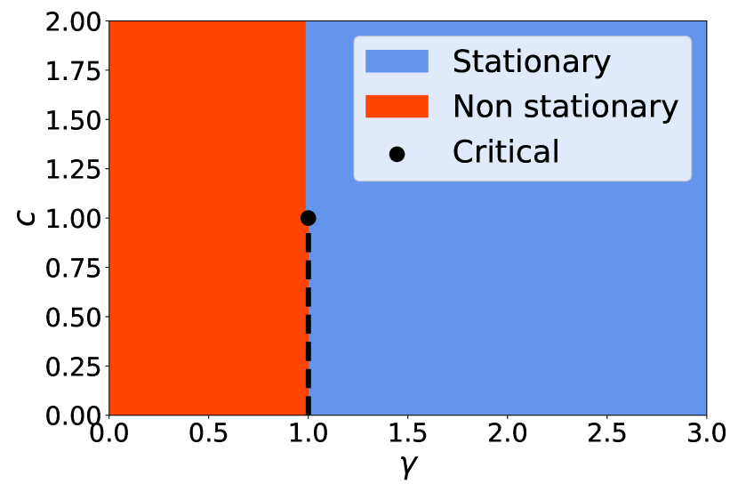
We start from the general recursion relation for $q_{k}(R)$ in Eq. (IV.2), valid for general $f(x)$. We assume that there exists a stationary solution $q(R)$ which would then satisfy the integral equation (32). Our strategy would be to find, for $f(x)$ given in Eq. (52), if Eq. (32) allows a normalizable solution $q(R)$. If it does not, there is no stationary solution. For later analysis, it is first convenient to define

$$q(R)=f(R)\,G(R)$$ (54)

and rewrite Eq. (32) as

$$G(R)=\int_{0}^{c}G(R^{\prime})\,f(R^{\prime})\,dR^{\prime}+\int_{c}^{R+c}\frac{G(R^{\prime})f(R^{\prime})}{1-F(R^{\prime}-c)}dR^{\prime}$$ (55)

where we recall $F(R)=\int_{0}^{R}f(y)dy$. By taking a derivative with respect to $R$ one gets

$$G^{\prime}(R)=\frac{f(R+c)}{1-F(R)}\,G(R+c)\,.$$ (56)

This is a first-order non-local differential equation. We need only one ‘boundary’ condition, i.e., the value of $G(R)$ at some point $R$, to fix the solution uniquely. To find such a condition, we note that the solution of this differential equation need, in addition, to satisfy the original integral equation (55). Substituting, e.g., $R=0$ in Eq. (55) gives a condition

$$G(0)=\int_{0}^{c}G(R^{\prime})\,f(R^{\prime})\,dR^{\prime}\,.$$ (57)

This shows that $G(0)$ is a constant and the solution must satisfy this condition (57) self-consistently. Another compatibility condition follows by investigating the large $R$ limit of Eq. (55). If the limit $G(\infty)$ exists, one obtains

$$G(\infty)=\int_{0}^{c}G(R^{\prime})\,f(R^{\prime})\,dR^{\prime}+\int_{c}^{\infty}\frac{G(R^{\prime})f(R^{\prime})}{1-F(R^{\prime}-c)}dR^{\prime}\,.$$ (58)

For arbitrary $f(x)$, it is hard to find a general solution to Eq. (56) with boundary condition (57) or (58). Hence, below we focus on the stretched exponential class in Eq. (52), for which the first-order equation (56) reduces to

$$G^{\prime}(R)=\frac{e^{-(R+c)^{\gamma}}}{\left[\int_{R}^{\infty}dR^{\prime}e^{-{R^{\prime}}^{\gamma}}\right]}\,G(R+c)\,.$$ (59)

Note that for $\gamma=1$, Eq. (59) reduces to $G^{\prime}(R)=e^{-c}\,G(R+c)$ and this leads to the nontrivial solution $q(R)=\lambda(c)\,e^{-\lambda(c)\,R}$ for all $R\geq 0$ with $\lambda(c)$ given in Eq. (44), as discussed in the previous section.

The case $c=0$ and arbitrary $\gamma>0$. Let us first start with $c=0$ case with arbitrary $\gamma>0$. In this case, Eq. (59) becomes local in $R$ whose general solution can be easily found

$$G(R)=G(R_{0})\,\frac{\int_{R_{0}}^{\infty}\,e^{-x^{\gamma}}\,dx}{\int_{R}^{\infty}\,e^{-x^{\gamma}}\,dx}\,,$$ (60)

where $R_{0}$ is arbitrary. The condition (57) says that for $c=0$, $G(0)=0$ identically. If we choose $R_{0}=0$ in Eq. (60), then using $G(0)=0$, we see that the only possible solution for $G(R)$ is just $G(R)=0$ for all $R$. Consequently, using Eq. (54), we get $Q(R)=0$ which evidently can not be normalized to unity. This indicates that there is no stationary solution $q(R)$ for $c=0$ and arbitrary $\gamma>0$. In other words, there is no stationary solution on the horizontal axis $c=0$ in the phase diagram in Fig. (9).

The case $0<\gamma<1$ and arbitrary $c>0$. In this case, we want to show that there is no limiting stationary solution $q(R)$ (see the (red) shaded region in the phase diagram in Fig. (9)). In other words, we will show that a solution to Eq. (56) satisfying the condition (58) does not exist for $\gamma<1$ with $c\geq 0$ arbitrary. To show this, it is sufficient to investigate Eq. (56) for large $R$, keeping $c\geq 0$ fixed. For large $R$, let us first assume that the limit $G(\infty)$ in Eq. (58) exists. Since $G(R)$ approaches a constant as $R\to\infty$, it follows that for any arbitrary $c\geq 0$ and large $R$, we must have $G(R+c)\to G(\infty)$ on the r.h.s of Eq. (56). This gives, for large $R$,

$$G^{\prime}(R)\approx G(\infty)\,\frac{e^{-(R+c)^{\gamma}}}{\left[\int_{R}^{\infty}dR^{\prime}\,e^{-{R^{\prime}}^{\gamma}}\right]}\,.$$ (61)

Now consider first the large $R$ behavior of the denominator on the r.h.s of Eq. (61). It is easy to show that, to leading order for large $R$,

$$\int_{R}^{\infty}e^{-{R^{\prime}}^{\gamma}}\,dR^{\prime}\approx\frac{1}{\gamma}\,R^{\gamma-1}\,e^{-R^{\gamma}}\,.$$ (62)

Substituting this in Eq. (61) one obtains for large $R$ and for any $\gamma>0$

$$G^{\prime}(R) \approx G(\infty)\,\gamma\,R^{\gamma-1}\,e^{-(R+c)^{\gamma}+R^{\gamma}}$$ (63)

$$\approx G(\infty)\,\gamma\,R^{\gamma-1}\,e^{-\gamma\,c\,R^{\gamma-1}}\,.$$

Consider now the case $0<\gamma<1$. In this case, the argument of the exponential on the r.h.s of Eq. (63) vanishes, i.e., $e^{-\gamma\,c\,R^{\gamma-1}}\to 1$ as $R\to\infty$. Consequently, integrating Eq. (63), one finds that $G(R)\sim R^{\gamma}$ actually grows with increasing $R$ for $\gamma<1$. But this is incompatible with the condition (58) and our starting assumption $G(\infty)$ is finite. In fact, this is also incompatible with the original integral equation (55). As $R\to\infty$, the l.h.s of Eq. (55) grows as $R^{\gamma}$, while the r.h.s approaches a constant since the integral on the r.h.s is convergent as $R\to\infty$. Hence we conclude that for $0<\gamma<1$ and $c\geq 0$, there is no stationary solution for $G(R)$, and equivalently for $q(R)$ leading to the (red) shaded area of the phase diagram in Fig. (9).

The case $\gamma>1$ and arbitrary $c>0$. Let us first check that in this case there is no obvious incompatibility between the large $R$ behavior in Eq. (63) and the original integral equation (55). Indeed, for $\gamma>1$, the exponential factor $e^{-\gamma\,c\,R^{\gamma-1}}$ on the r.h.s of Eq. (63) decays rapidly, and integrating over $R$ we find that $G(R)$ approaches a constant as $R\to\infty$, which is perfectly compatible with Eq. (55) in the large $R$ limit, or equivalently with Eq. (58). This already indicates that there is a normalizable stationary solution for any $c>0$ and $\gamma>1$. To compute explicitly this solution for arbitrary $c>0$ (and $\gamma>1$) still seems rather hard. Below, we compute this stationary distribution for $\gamma>1$ in two opposite limits: (i) $c\to 0^{+}$ and (ii) $c\to\infty$ limit.

The limit $c\to 0^{+}$ and $\gamma>1$ arbitrary. We start with the $c\to 0$ limit with fixed $\gamma>1$. We fix $R$ in Eq. (59) and take the limit $c\to 0^{+}$. To leading order for small $c$, we can approximate $G(R+c)\approx G(R)$ to make Eq. (59) local and also expand $(R+c)^{\gamma}\approx R^{\gamma}+\gamma\,c\,R^{\gamma-1}$ up to $O(c)$ with $R$ fixed. Eq. (59) then reduces to

$$\frac{1}{G(R)}\,\frac{dG(R)}{dR}\approx\frac{e^{-R^{\gamma}-c\,\gamma\,R^{\gamma-1}}}{\left[\int_{R}^{\infty}dR^{\prime}\,e^{-{R^{\prime}}^{\gamma}}\right]}\equiv g_{c}(R)\,.$$ (64)

Note that only $c$-dependence appears through the factor $c\,gamma\,{R^{\prime}}^{\gamma-1}$ inside the exponential in $g_{c}(R)$. For $\gamma>1$, this term contributes significantly for large $R$, even when $c\to 0^{+}$. Hence, we can not neglect this $c$-dependent term, especially for large $R$. One can then easily integrate Eq. (64) and obtain the solution as

$$G(R)\approx G(0)\,\exp\left[\int_{0}^{R}g_{c}(x)\,dx\right]\,,$$ (65)

where $G(0)$ is a constant and $g_{c}(x)$ is defined in Eq. (64). It is easy to show that for large $x$, $g_{c}(x)$ behaves as $g_{c}(x)\approx\gamma\,x^{\gamma-1}\,e^{-\gamma\,c\,x^{\gamma-1}}$. Hence for $\gamma>1$, the integral $\int_{0}^{\infty}g_{c}(x)\,dx$ is perfectly convergent and is just a constant. Consequently, we find from Eq. (65) that $G(R)\to G(\infty)=G(0)\,\exp\left[\int_{0}^{\infty}g_{c}(x)\,dx\right]$ as $R\to\infty$. Thus the stationary solution $q(R)$ in this $c\to 0^{+}$ limit is given by

$$q(R)\approx\frac{\gamma}{\Gamma\left(\frac{1}{\gamma}\right)}\,e^{-R^{\gamma}}\,G(R)\approx f(R)\,G(R)$$ (66)

where the function $G(R)$, given in Eq. (65), is well defined for any $R$ as long as $c\to 0^{+}$ (nonzero) and $\gamma>1$. Thus, in the $c\to 0$ limit, the stationary record value distribution $q(R)$ gets modified considerably from the parent distribution $f(R)$ by the multiplicative factor $G(R)$.

The limit $c\to\infty$ and $\gamma>1$ arbitrary. Next we consider the opposite limit $c\to\infty$. When $c\to\infty$ every random variable in the series $\{x_{1},\,x_{2},\,x_{3},\,\cdots\}$ is a record, hence $q(R)=f(R)$ and $G(R)=1$ for all $R\geq 0$. Now consider $c$ large, but not strictly infinite. In this case, the function $G(R)$ will change from its flat value $G(R)=1$ that is valid strictly for $c\to\infty$. However, we expect that $G(R)$, in the limit $R\to\infty$, is not very sensitive to $c$, i.e., $G(\infty)=1$ even for finite but large $c$. However, for finite but fixed $R$, we expect that $G(R)$ will deviate from its flat value $1$. To find this change in $G(R)$ for fixed $R$, to leading order for large $c$, we can use the approximation $G(R+c)\approx 1$ on the r.h.s of Eq. (59) and solve the resulting first-order local equation, leading to the solution

$$G(R)=1-\int_{R}^{\infty}\frac{e^{-(R^{\prime}+c)^{\gamma}}}{\left[\int_{R^{\prime}}^{\infty}e^{-x^{\gamma}}dx\right]}\,dR^{\prime}\,,$$ (67)

where we used the expected boundary condition $G(\infty)=1$ mentioned above. For fixed $R$ and large $c$, we can approximate $(R+c)^{\gamma}\approx c^{\gamma}+\gamma\,c^{\gamma-1}\,R$. Using this approximation in the numerator of the integrand in Eq. (67) and rescaling $z=\gamma\,c^{\gamma-1}\,R^{\prime}$, we find that for $\gamma>1$ and in the scaling limit $c\to\infty$, $R\to 0$ such that the product $c^{\gamma-1}\,R$ is fixed

$$G(R)\approx 1-\frac{e^{-c^{\gamma}}}{c^{\gamma-1}\,\Gamma(\frac{1}{\gamma})}\,e^{-\gamma c^{\gamma-1}\,R}\,.$$ (68)

This is clearly compatible with the starting ansatz that $G(\infty)=1$. Finally, using this in Eq. (54) we get the stationary solution for $\gamma>1$ and large $c$ limit

$$q(R)\approx f(R)\,\left[1-\frac{e^{-c^{\gamma}}}{c^{\gamma-1}\,\Gamma(\frac{1}{\gamma})}\,e^{-\gamma c^{\gamma-1}\,R}\right]\,.$$ (69)

Thus, in the $c\to\infty$ limit, $q(R)$ approaches $f(R)$ with a small additive corection term as given in Eq. (69).

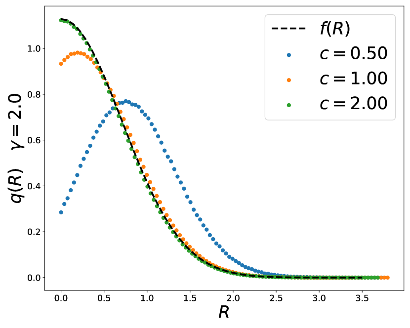
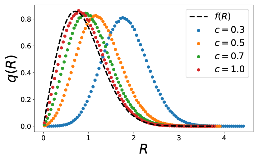
Summarizing, for $\gamma>1$ in the phase diagram in Fig. (9), the record value distribution becomes stationary for large $k$, for any $c>0$. In the two limits $c\to 0$ and $c\to\infty$, the stationary distribution $q(R)$ is given respectively in Eqs. (66) and (69). We have checked these results numerically in Fig. (10) for $\gamma=2$. In this figure, we see that as $c$ increases, $q(R)$ progressively approaches $f(R)$.

Figure 10: Stretched exponential case: stationary record distributions $q(R)$ at $\gamma=2$ and for different $c$. As $c$ gets bigger, $q(R)$ approaches $f(R)$.

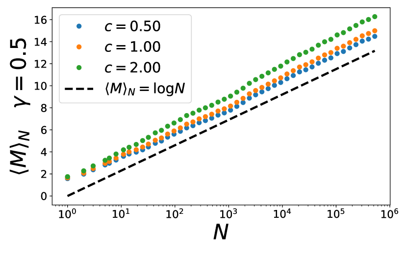
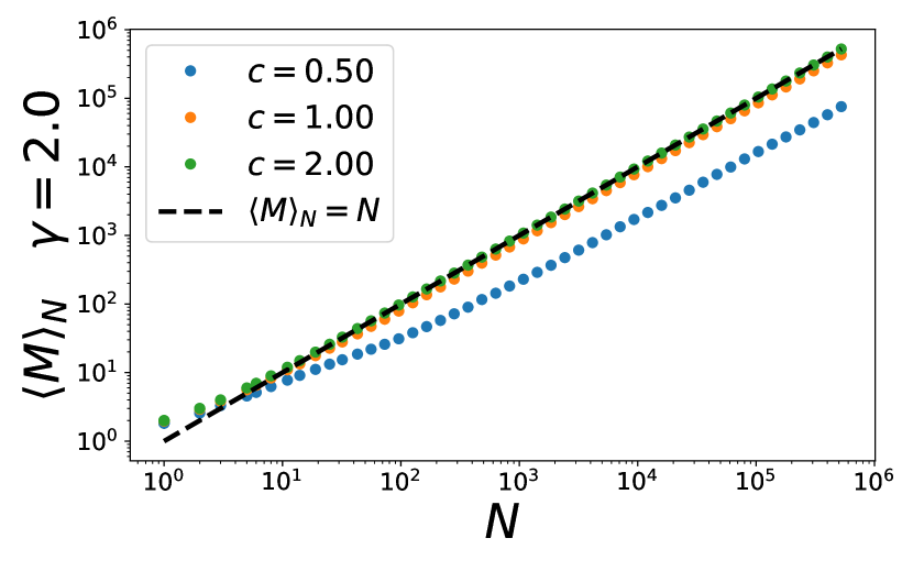
We have also computed numerically the mean number of records $\langle M_{N}\rangle$ up to $N$ steps. As indicated in the phase diagram in Fig. (9), we expect that for $0<\gamma<1$ the record process is non-stationary, i.e., the effect of $c$ is insignificant and the system behaves similar to $c=0$. Hence in this regime ((red) shaded region in the phase diagram in Fig. (9), we expect $\langle M_{N}\rangle\simeq\ln N$ for large $N$, for any $c>0$. This prediction is verified numerically in Fig. (11), for $\gamma=1/2$ and for several values of $c$. In contrast, for $\gamma>1$ and $c>0$ ((blue) shaded region in the phase diagram in Fig. (9)), we have a stationary phase. In this case, we expect a linear growth $\langle M_{N}\rangle\simeq A_{1}(c)\,N$ for large $N$, with an $c$-dependent amplitude $A_{1}(c)\leq 1$. In the limit $c\to\infty$, we expect $A_{1}(c)\to 1$, since every entry becomes a record in this limit. In Fig. (12), we verify this prediction for fixed $\gamma=2$ and for several values of $c$.

Figure 11: Stretched exponential case: logarithmic growth of the mean number of $c$-records for different $c$ and $\gamma=0.50$. The dashed line is a guide to the eye.

Figure 12: Stretched exponential case: linear growth of the mean number of $c$-records for different $c$ and $\gamma=2$.

VII Other distributions

In this section, we study other classes of $f(x)$. First we consider the uniform distribution of $f(x)$ over the bounded interval $[0,1]$ for which we present exact analytical results for all three observables $\langle M_{N}\rangle$, $q_{k}(R)$ and $\pi_{k}(n)$. We then consider more general bounded distributions. Bounded distributions belong to the family of $f(x)$ with a ‘faster than’ exponential tail, hence we anticipate and demonstrate below that both $q_{k}(R)$ and $\pi_{k}(n)$ allow stationary limiting distributions as $k\to\infty$ for bounded $f(x)$. We then consider another class of unbounded distribution, which we call the Weibull class

$$f_{\text{Weibull}}(x)=\gamma\,x^{\gamma-1}\,e^{-x^{\gamma}}\,\quad{\rm for}\,\,\gamma>0$$ (70)

with $F_{Weibull}(x)=1-e^{-x^{\gamma}}$. It turns out that this $f(x)$ is easier to sample numerically using the inverse Transform method, as explained in the appendix (G). We present detailed numerical results for all three observables $\langle M_{N}\rangle$, $q_{k}(R)$ and $\pi_{k}(n)$ for this case.

VII.1 Bounded distributions

The $c$-record process associated to I.I.D time series drawn from bounded distributions has a well defined stationary limit for any $c>0$. For simpicity we restrict the interval to the segment $[0,1]$. This implies that for any $c>1$, every entry $x_{i}$ of the time series is a record.

VII.2 Uniform distribution

We first consider the uniform distribution $f(x)=\mathbb{I}_{[0,1]}(x)$ and show that the mean number of records, the stationary record distribution and their age distribution can be explicitly computed for $1/2\leq c\leq 1$. For $0<c<1/2$. the calculations are more cumbersome and we rely on Monte Carlo simulations.

To computed the mean number of records we study equation (25) for the uniform distribution. Its expression simplifies to:

$$\tilde{Q}(R)\left[1-z(R-c)\theta(R-c)\right]=\\ =z\,s+z\,s\,\int_{0}^{\min(1,R+c)}\tilde{Q}(R^{\prime})dR^{\prime}$$ (71)

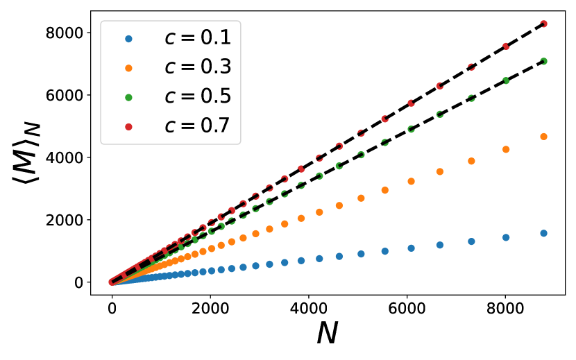
This equation is solved in appendix (D) for $1/2\leq c\leq 1$ and the exact mean number of records reads:

$$\langle M\rangle_{N}=(2-c+\ln(c))N+\frac{1-c}{c}+\ln(c)$$ (72)

Note that when $c=1$, we get $\langle M\rangle_{N}=N$ as expected. In Fig. (13) we numerically computed $\langle M\rangle_{N}$ for different values of $c$ and included the analytical predictions for $1/2\leq c\leq 1/2$.

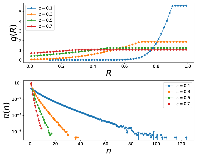
The stationary record distribution $q(R)$ satisfies Eq. (41) together with the condition that $q(R)=0$ for $R>1$:

$$q^{\prime}(R)=\begin{cases}0&\quad\;1-c<R<1\\ &\\ \frac{q(R+c)}{1-R}&\quad\;0<R<1-c\end{cases}$$ (73)

Eq. (73) is valid for any $0\leq c\leq 1$. For $c\geq 1/2$, it can be simply solved. In particular, imposing the global normalization, one gets:

$$q(R)=\frac{1}{2-c+\ln(c)}\begin{cases}1&1-c<R<1\\ 1-\ln\frac{1-R}{c}&0<R<1-c\end{cases}$$ (74)

In Fig. (14) (upper panel) we show $q(R)$ for different values of $c$ along with the analytical predictions for $1/2\leq c\leq 1$.

The stationary age distribution $\pi(n)$ (for $1/2\leq c\leq 1$) follows from Eqs. (IV.3) and (74):

$$\pi(n)=\frac{1+\ln(c)}{2+\ln(c)-c}\delta_{n,1}+\\ +\frac{1}{2+\ln(c)-c}\frac{(1-c)^{n}}{n}\left[1-\frac{n(1-c)}{n+1}\right]$$ (75)

$\pi(n)$ shows a delta peak at $n=1$, as in the exponential case. For large $n$, $\pi(n)$ decays exponentially over a characteristic scale $-1/\ln(1-c)$ that gets smaller as $c\to 1$. The fact that $\pi(n)$ has a well defined first moment is compatible with the scaling of the average number of records, namely $\langle M\rangle_{N}\propto N$ as $N\to\infty$.

Figure 13: Uniform case: mean number of $c$-records for different $c$. For $c\geq 1/2$ we include the analytical predictions in Eq. (72) as shown by dashed lines. The agreement is excellent.

Figure 14: Record (upper panel) and age (lower panel) distributions for various $c$ for the uniform distribution. Analytical results of Eqs. (74) and (75) are shown by solid lines in the upper panel.

VII.3 Generic bounded distributions

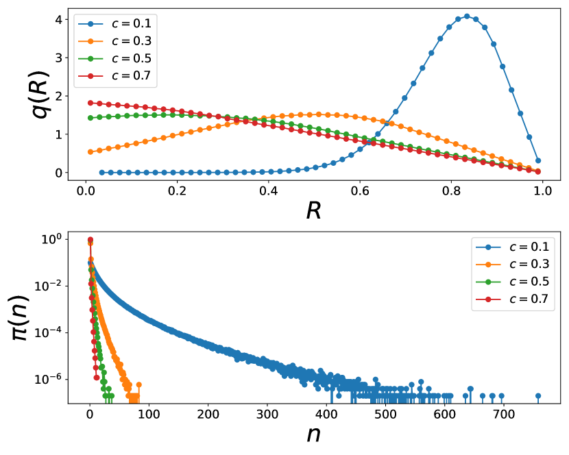
The $c$-record process associated to a generic bounded distribution is more difficult to characterize analytically. However some of the features that we found for the case of the uniform distribution remain valid. In particular for any value of $c$ the mean number of records grows linearly with $N$ (at large $N$) and the stationary distribution of ages displays an exponential cutoff. As an illustration we studied numerically the family of distribution wth cumulative $F(x)=1-(1-x)^{\nu}$. The uniform distribution corresponds to $\nu=1$. In Fig. (15) we report our results for $\nu=2$: in the upper panel the study of the stationary record distribution $q(R)$ and in the lower panel the age distribution $\pi(n)$.

Figure 15: Record (upper panel) and ages (lower panel) distributions for various $c$ for the bounded case with cumulative distribution $F(x)=1-(1-x)^{2}$ with $0\leq x\leq 1$.

VII.4 Numerical results for the Weibull family

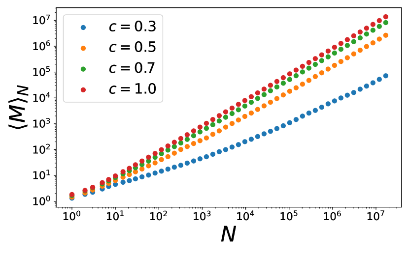
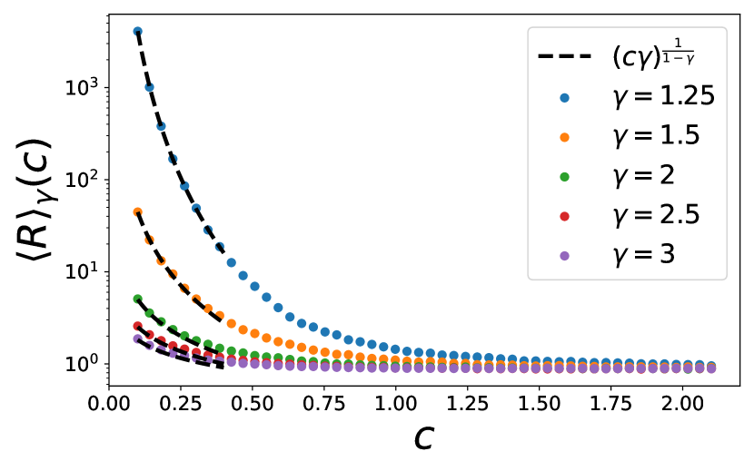
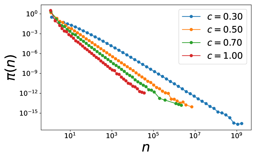
In this section we briefly summarize the numerical results for $\langle M\rangle_{N}$ $q(R)$, $\pi(n)$ for the Weibull family. In Fig. (16) we show the mean number of records $\langle M\rangle_{N}$ as a function of $N$ for $10^{3}$ realizations of the $c$-record process. For large enough $N$ the scaling $\langle M\rangle_{N}\propto N$ is recovered. In Fig. (17) we show the stationary record distribution for the Weibull distribution at $\gamma=2$. We find a stationary distribution for any $c>0$. As $c$ gets bigger, $q(R)$ approaches $f(R)$, as expected. In Fig. (18) we show the average record $\langle R\rangle_{\gamma}(c)$ as a function of $c$ for different $\gamma$’s. We also insert the scaling as $c\to 0^{+}$ of the average record value obtained using the argument in appendix F:

$$\langle R\rangle_{\gamma}(c)\approx(c\gamma)^{\frac{1}{\gamma-1}}$$ (76)

Finally Fig. (19) shows the age of record distributions at $\gamma=2$ for different values of $c$. The distributions have a power law decay as $n\to\infty$ with an exponent $\tau\geq 2$, i.e., $\pi(n)\sim n^{-\tau}$. This numerical result is compatible with the scaling $\langle M\rangle_{N}\propto N$ of the average number of records since a power law with $\tau\geq 2$ has a well defined first moment.

Figure 16: Weibull case with $\gamma=2$: mean number of $c$-records for various $c$. As $c$ gets smaller, the converges to $\langle M\rangle_{N}\propto N$ is

Figure 17: Record distributions for the Weibull family with $\gamma=2$ for various $c$.

Figure 18: Average record value for various $\gamma$ and $c$ for the Weibull family. We plot with the dashed black line the expected scaling of the average for $c\to 0^{+}$ (see Eq. (76)).

Figure 19: Age of record numerical distributions for the Weibull family at $\gamma=2$ and varying $c$. All the distributions show a power law tail with exponent $\geq 2$.

VIII Generalizations of the record process

Before the conclusion we would like to discuss some possible generalizations of the $c$-record problem. For simplicity here we focus only on the conditions for the existence of a stationary record distribution and on its form. We let the calculations of the mean number of records and of the age statistics to future works. Few protocols can be considered as a straightforward generalization of the $c$-record process:

• The constant $c$ can be promoted to be a positive random variable with distribution $g(c)$. For $f(x)=e^{-x}\theta(x)$ the fixed point equation for the stationary record distribution, averaged over all possible values of $c$ (annealed average), writes:

  $$q^{\prime}(R)=\int_{0}^{\infty}g(c)q(R+c)dc-q(R)$$ (77)

  Remarkably this equation admits an exponential solution $q(R)=\lambda e^{-\lambda R}$ if the equation

  $$1-\lambda=\tilde{g}(\lambda)\equiv\int_{0}^{\infty}e^{-\lambda c}g(c)dc$$ (78)

  has a positive solution $\lambda$. For example if $g(c)$ is an exponential distribution, a stationary state is reached if its mean is bigger than $1$.

• The definition of the $c$-record can be extended with a function $c(R)$, namely $R_{k}$ is a record if $R_{k}>R_{k-1}-c\,(R_{k-1})$. As a concrete example one can consider $c(R)=c\,R$ with $c<1$ (for $c\geq 1$ all the values of the time series are records):

  $$R_{k}>(1-c)\,R_{k-1}$$ (79)

  The fixed point equation for the stationary record distribution $q(R)$ satisfies:

  $$q^{\prime}(R)=\frac{f(R)}{1-F(R)}\frac{1}{1-c}q\left(\frac{R}{1-c}\right)+$$ (80)

  $$+\frac{f^{\prime}(R)}{f(R)}q(R)$$

  Equation (80) becomes simple for a Pareto distribution $f(x)=\frac{\alpha}{x^{\alpha+1}}\theta(x-1)$:

  $$q^{\prime}(R)=\frac{\alpha}{R(1-c)}q\left(\frac{R}{1-c}\right)-\frac{\alpha+1}{R}q(R)$$ (81)

  The stationary state exists for $c>1-e^{-\frac{1}{\alpha}}$ and the solution of (81) still a Pareto distribution $q(R)=\frac{\beta}{R^{\beta+1}}\theta(R-1)$ with $\beta$ the unique positive solution of the trascendental equation

  $$1-\frac{\beta}{\alpha}=(1-c)^{\beta}$$ (82)

  The records generated by this process are equivalent to the $c$-records discussed in this paper via the map $R_{k}\to\ln R_{k}$. Under this mapping the Pareto distribution becomes the exponential distribution.

• Finally we consider the following $k$-dependent record condition:

  $$R_{k}>R_{k-1}-c(k+1)^{b-1}$$ (83)

  for a constant $b>0$. This protocol has been considered in PK16 in the context of evolutionary biology: the quantity $c(k+1)^{b-1}$ is called handicap and the analysis is carried out for both increasing $b>1$ and decreasing $b<1$ handicaps. The case $b=1$ coincides with the $c$-record process. We refer the reader to the original work PK16 for details.

IX Conclusion

In this paper, we have shown that a simple record model of an I.I.D series, which we call the $c$-record model, can be successfully used to understand and explain several realistic features of avalanche statistics in disordered systems, an example being the earthquake dynamics in seismicity. This model has a single parameter $c\geq 0$ and the other input is the distribution $f(x)$ of an entry. We have focused on three natural observables: (i) the mean number of records $\langle M_{N}\rangle$ up to step $N$ in an infinite series (ii) the distribution $q_{k}(R)$ of the value of the $k$-th record and (iii) the distribution $\pi_{k}(n)$ of the time interval $n$ between the $k$-th and the $(k+1)$-th record.

One of our main conclusions is that if $f(x)$ decays, for large $x$, slower than an exponential, both $q_{k}(R)$ and $\pi_{k}(n)$ do not have stationary limits as $k\to\infty$ and $\langle M_{N}\rangle\sim\ln N$ for large $N$, as in the $c=0$ case. Thus the effect of $c$ is not very significant for $f(x)$ with a slower than exponential tail. In contrast, if $f(x)$ has a faster than exponential tail, both $q_{k}(R)\to q(R)$ and $\pi_{k}(n)\to\pi(n)$ approach stationary limiting forms as $k\to\infty$. In particular, we show that $\pi(n)$ decays faster than $1/n^{2}$ for large $n$ (indicating that $\langle n\rangle$ is finite). Additionally, in this case, the mean number of records grows linearly as $\langle M_{N}\rangle\sim A_{1}(c)\,N$ for large $N$ with $A_{1}(c)\leq 1$. Thus, for $f(x)$ decaying faster than exponential, the statistics of these three observables for finite $c$ are fundamentally different from the standard $c=0$ case. When $f(x)$ has an exponential tail, it turns out to be a marginal case where there is a phase transition at a critical value $c_{\rm crit}$. For $c<c_{\rm crit}$, the observables have qualitaively similar behavior as the $c=0$ case. In contrast for $c>c_{\rm crit}$, both $q_{k}(R)$ and $\pi_{k}(n)$ have stationary limits as $k\to\infty$. We have illustrated by an explicit calculation for $f(x)=e^{-x}\theta(x)$ for which $c_{\rm crit}=1$. In this case we have shown that for $c>1$, the stationary avalanche size distribution $\pi(n)\sim n^{-1-\lambda(c)}$ has a power law tail for large $n$ with $\lambda(c)\leq 1$, indicating that the first moment diverges. Remarkably, the exponent $\lambda(c)$ depends continuously on $c$ and is given by the root of the transcendental equation, $c=-\ln(1-\lambda)/\lambda$. We have also computed exactly the stationary record value distribution $q(R)$ for $c>1$ and shown that it is a pure exponential, $q(R)=\lambda(c)\,e^{-\lambda(c)\,R}$, for all $R\geq 0$.

An important feature of this $c$-record model is a nontrivial correlation structure between record values, as well as between record intevals. In this paper we have explored only partially this structure, and it would be interesting to characterize this correlation structure in a more complete fashion.

We have also provided some generalisations of this simple $c$-record model, where the criteria for record formation, i.e., the offset $c_{k}$ depends on the record value $R_{k}$ as well as on the record index $k$. In all these cases, the offset $c_{k}$ remains constant (albeit $k$-depenent) as in the lower panel of Fig. (3). Previously, the linear trend model was studied where the offset decreases linearly with time during an avalanche (as in the upper panel of Fig. (3)). One can then ask how the record statistics gets modified for a general decreasing offset function during an avalanche.

Finally, in this paper, we have considered a series of I.I.D variables as a model for the pinning force landscape. It is natural to consider a model where the landscape is correlated. For example, in the ABBM model, the entries of the series correspond to the positions of a random walker. This remains a challenging open problem.

Appendix A Exponential case: $P_{N}(M,R)$

Our starting point is Eq. (35) for the generating function ${\tilde{Q}}(R)$ in the exponential case, $f(x)=e^{-x}\,\theta(x)$. We solve it in terms of $H(R)=\int_{0}^{R}\tilde{Q}(R^{\prime})dR^{\prime}$. Thus Eq. (35) becomes:

$$H^{\prime}(R)\left[1-z(1-e^{-(R-c)})\theta(R-c)\right]=\\ z\,s\,e^{-R}\,\left[1+H(R+c)\right]$$ (84)

The initial condition for $H(R)$ is $H(0)=0$. In order to solve (84) we need to distinguish region I with $R<c$, region II with $R>c$ and match the two solutions at $R=c$. We call $H_{I}(R)$ the solution for region I and $H_{II}(R)$ the one for region II.

We start with region II ($R>c$) and use the ansatz

$$H_{II}(R)=\sum_{m=0}^{\infty}a_{m}e^{-m\,R}$$ (85)

Substituting this in Eq. (84) and matching terms of $e^{-R}$ on both sides, we get the following recursion relation for the coefficients $a_{m}$’s

$$a_{1}=-\frac{zs}{1-z}(1+a_{0})$$ (86)

$$a_{m}=-\frac{ze^{c}}{1-z}\left(\frac{m-1+se^{-mc}}{m}\right)a_{m-1}\,.$$ (87)

By iterating we get

$$a_{m}=(-1)^{m}\left(\frac{ze^{c}}{1-z}\right)^{m}\frac{1}{m!}b_{m}(s)(1+a_{0})$$ (88)

where

$$b_{m}(s)=\begin{cases}\prod_{k=1}^{m}(k-1+se^{-kc})&m\geq 1\\ 1&m=0\end{cases}$$ (89)

We then rewrite $H_{II}(R)$ as

$$H_{II}(R)=(1+a_{0})\sum_{m=0}^{\infty}\left(-\frac{ze^{c}}{1-z}\right)^{m}\frac{b_{m}(s)}{m!}e^{-mR}\,.$$ (90)

The coefficient $a_{0}$ is a parameter that must be set by imposing the matching of $H_{I}(R)$ and $H_{II}(R)$ at $R=c$. In the region I, $H_{I}(R)$ satisfies:

$$(1-z)\frac{dH_{I}(R)}{dR}=zse^{-R}(1+H_{II}(R+c))$$ (91)

Substituting the solution of $H_{II}(R)$ from Eq. (90) on the r.h.s of (91) and solving the first order equation for $H_{I}(R)$, using $H_{I}(0)=0$, gives

$$H_{I}(R)=sz(1+a_{0})\sum_{m=0}^{\infty}\left(-\frac{z}{1-z}\right)^{m}\\ \frac{b_{m}(s)}{(m+1)!}\frac{(1-e^{-(m+1)R})}{m+1}$$ (92)

The continuity at $R=c$, namely $H_{I}(c)=H_{II}(c)$, fixes $a_{0}$:

$$a_{0}=\frac{1}{\sum_{m=0}^{\infty}\left(-\frac{z}{1-z}\right)^{m}\frac{b_{m}(s)}{m!}\left(1-\frac{zs(1-e^{-(m+1)c})}{m+1}\right)}-1$$ (93)

In the limit $R\to\infty$, we have $H(\infty)=\int_{0}^{\infty}{\tilde{Q}}(R^{\prime})\,dR^{\prime}$. On the other hand, it follows by taking $R\to\infty$ limit in Eq. (85) that $H(\infty)=a_{0}$. Combining these two and using Eq. (27), we finally identify:

$$\sum_{N=1}^{\infty}\sum_{M=1}^{\infty}P_{N}(M)z^{N}s^{M}=a_{0}=a_{0}(z,s)\,,$$ (94)

with $a_{0}$ given in Eq. (93). One can check that for $c=0$

$$a_{0}=\frac{1}{(1-z)^{s}}-1$$ (95)

which reproduces the well known result for the generating function of the standard record process GMS17 . To find the generating function of $\langle M\rangle_{N}$ one must study $a_{0}$ in the vicinity of $s=1$. The expansion around $s=1$ from (93) is not straightforward. We want to rewrite the denominator of $a_{0}$ in a simpler form using $\tilde{b}(x,s)$, the generating function of $b_{m}(s)$. We first introduce an useful identity:

$$\tilde{b}(x,s)=\sum_{m=0}^{\infty}\frac{b_{m}(s)}{m!}x^{m}$$

$$=1+\sum_{m=1}^{\infty}(m-1+se^{-mc})\frac{b_{m-1}(s)}{m!}x^{m}=$$

$$=1+\sum_{m=1}^{\infty}\frac{b_{m-1}(s)x^{m}}{(m-1)!}-\sum_{m=1}^{\infty}\frac{b_{m-1}x^{m}}{m!}+$$

$$+s\sum_{m=1}^{\infty}\frac{b_{m-1}(xe^{-c})^{m}}{m!}$$

$$=1+x\tilde{b}(x,s)-\sum_{m=1}^{\infty}\frac{b_{m-1}x^{m}}{m!}+$$

$$+s\sum_{m=1}^{\infty}\frac{b_{m-1}(xe^{-c})^{m}}{m!}\,.$$ (96)

Eq. (A) can be rewritten as:

$$(1-x)\tilde{b}(x,s)=1-\sum_{m=1}^{\infty}\frac{b_{m-1}(s)x^{m}}{m!}+s\sum_{m=1}^{\infty}\frac{b_{m-1}(s)(xe^{-c})^{m}}{m!}$$ (97)

We now identify $x=-z/(1-z)$ and thus $z=-x/(1-x)$. Using Eq. (97), the denominator of Eq. (93) can be rewritten as:

$$\sum_{m=0}^{\infty}\frac{x^{m}}{m!}b_{m}(s)+\frac{xs}{1-x}\sum_{m=0}^{\infty}\frac{b_{m}(s)x^{m}}{m!(m+1)}\left[1-e^{-(m+1)c}\right]$$

$$=\tilde{b}(x,s)+\frac{xs}{1-x}\sum_{m=0}^{\infty}\frac{b_{m}(s)x^{m}}{(m+1)!}-\frac{xse^{-c}}{1-x}\sum_{m=0}^{\infty}\frac{b_{m}(s)(xe^{-c})^{m}}{(m+1)!}$$

$$=\tilde{b}(x,s)+\frac{s}{1-x}\sum_{m=1}^{\infty}\frac{b_{m-1}x^{m}}{m!}+$$

$$-\frac{1}{1-x}\left[(1-x)\tilde{b}(x,s)-1+\sum_{m=1}^{\infty}\sum_{m=1}^{\infty}\frac{b_{m-1}x^{m}}{m!}\right]$$

$$=\frac{1}{1-x}\left[1-(1-s)\sum_{m=1}^{\infty}\frac{b_{m-1}(s)x^{m}}{m!}\right]$$ (98)

Reintroducing $z=-x/(1-x)$, we rewrite Eq. (93) in a more amenable form to carry out the expansion around $s=1$:

$$1+a_{0}=\frac{1}{(1-z)\left[1-(1-s)\sum_{m=1}^{\infty}\frac{b_{m-1}(s)}{m!}\left(-\frac{z}{1-z}\right)^{m}\right]}$$ (99)

By expanding $a_{0}$ in $s=1-\epsilon$ as $\epsilon\to 0$ we can extract the derivative of $a_{0}$ in $s=1$. After some algebra we finally arrive at the generating function of $\langle M\rangle_{N}$:

$$\tilde{M}(z)=\sum_{N=1}^{\infty}\langle M\rangle_{N}z^{N}=\left.\frac{\partial a_{0}}{\partial s}\right|_{s=1}=\\ =-\frac{1}{1-z}\sum_{m=0}^{\infty}\frac{b_{m}(1)}{(m+1)!}\left(-\frac{z}{1-z}\right)^{m+1}$$ (100)

In accordance to Eq. (28), the average number of records $\langle M\rangle_{N}$ identifies with the coefficient $z^{N}$ in the series expansion of $\tilde{M}(z)$ at $z=0$. The explicit expression of $\langle M\rangle_{N}$ is given in Eq. (36).

Appendix B Asymptotics of $\langle M\rangle_{N}$

From now on $b_{m}=b_{m}(1)$ and $\tilde{b}(x)=\tilde{b}(x,1)$. The behavior of $\langle M\rangle_{N}$ for $N\to\infty$ is hard to extract from Eq. (36). It is then useful to restart from Eq. (100) and introduce the function $\tilde{g}(x)$ such that:

$$\tilde{M}(z)=-\frac{1}{1-z}\tilde{g}\left(-\frac{z}{1-z}\right)$$ (101)

The function $\tilde{g}(x)$ writes:

$$\tilde{g}(x)=\sum_{m=0}^{\infty}b_{m}\frac{x^{m+1}}{(m+1)!}$$ (102)

The asymptotics of $\langle M\rangle_{N}$ for large $N$ is controlled by the behavior of $\tilde{M}(z)$ when $z\to 1$, which is equivalent to $\tilde{g}(x)$ when $x\to-\infty$. By the definition of $\tilde{b}(x)$ (A) it is straightforward to note that:

$$\frac{d\tilde{g}(x)}{dx}=\tilde{b}(x)$$ (103)

Setting $s=1$ in Eq. (97) gives

$$(1-x)\tilde{b}(x)=1-\sum_{m=1}^{\infty}\frac{b_{m-1}x^{m}}{m!}+\sum_{m=1}^{\infty}\frac{b_{m-1}(xe^{-c})^{m}}{m!}\,.$$ (104)

We can derive two differential equation for $\tilde{g}(x)$ and $\tilde{b}(x)$: The first is obtained by rewriting each term of (104) using $\tilde{g}(x)$:

$$(1-x)\frac{d\tilde{g}(x)}{dx}=1-\tilde{g}(x)+\tilde{g}(xe^{-c})$$ (105)

The second is obtained from the derivative of (104) with respect to $x$:

$$\frac{d\tilde{b}(x)}{dx}=\frac{e^{-c}\tilde{b}(e^{-c}x)}{1-x}$$ (106)

Note that Eq. (106) is a first order non-local differential equation. The representation of $\tilde{b}(x)$ given in Eq. (A) is not suitable for studying the limit $x\to-\infty$. Instead the solution of (106) gives us a nice series representation of $\tilde{b}(x)$ around $x\to-\infty$ using the following ansatz:

$$\tilde{b}(x)=\sum_{k=0}^{\infty}A_{k}(-x)^{-\phi-k}$$ (107)

By plugging the ansatz in (106) we find that coefficients satisfy:

$$A_{k}=\frac{k-1+\phi}{e^{ck}\phi-k-\phi}A_{k-1}$$ (108)

with $A_{0}$ to be determined. The exponent $\phi$ is the solution of:

$$\phi=(e^{-c})^{1-\phi}$$ (109)

At most two solutions exist for (109).

• For $c<1$ one solution is $\phi=1$ and the other is $\phi(c)>1$.

• For $c>1$ one solution is $\phi=1$ and the other is $\phi(c)<1$

• For $c=1$ the two solutions coincide i.e. $\phi=1$.

From now on we assume $c\neq 1$ and rewrite the ansatz (107) in order to make explicit the existence of two solutions:

$$\tilde{b}(x)=A_{0}\sum_{k=0}^{\infty}\frac{c_{k}}{(-x)^{\phi+k}}+B_{0}\sum_{k=0}^{\infty}\frac{\tilde{c}_{k}}{(-x)^{k+1}}$$ (110)

where:

$$c_{k}=\prod_{m=1}^{k}\frac{m-1+\phi}{(e^{cm}-1)\phi-m}$$ (111)

and:

$$\tilde{c}_{k}=\prod_{m=1}^{k}\frac{m}{e^{cm}-m-1}$$ (112)

with $c_{0}=\tilde{c}_{0}=1$. Both $c_{k}$ and $\tilde{c}_{k}$ come from the iteration of equation (108). To complete the solution we have to find $A_{0}$ and $B_{0}$. Before that we note that identifying $\phi(c)=1-\lambda(c)$ equation (44) is equivalent to (109). The case $c>1$ corresponds to a positive $\lambda(c)$, to the existence of a stationary state and when $x\to-\infty$ to $\tilde{b}(x)\sim A_{0}(-x)^{-\phi}$. While when $c<1$ no stationary state exists and $\tilde{b}(x)\sim B_{0}/(-x)$.

To set $A_{0}$ and $B_{0}$ we need two relations. The first relation is found by matching at $x=-1$ the value of $\tilde{b}(x)$ in the two series representation given by (A) and (110):

$$\tilde{b}(-1)=\sum_{m=0}^{\infty}(-1)^{m}\frac{b_{m}}{m!}=A_{0}\sum_{k=0}^{\infty}c_{k}+B_{0}\sum_{k=0}^{\infty}\tilde{c}_{k}$$ (113)

From the solution (110) we can find, up to an integration constant $\mu(c)$, $\tilde{g}(x)$:

$$\tilde{g}(x)=A_{0}\sum_{k=0}^{\infty}\frac{c_{k}(-x)^{-\phi-k+1}}{\phi+k-1}+B_{0}(-\ln(-x))+$$

$$+B_{0}\sum_{k=1}^{\infty}\tilde{c}_{k}\frac{(-x)^{-k}}{k}+\mu(c)\,.$$ (114)

The second relation corresponds to imposing that Eq. (B) must be a solution of (105):

$$(1-x)\left[A_{0}\sum_{k=0}^{\infty}c_{k}(-x)^{-\phi-k}+B_{0}\sum_{k=0}^{\infty}\tilde{c}_{k}(-x)^{-k-1}\right]=\\ =1-\left[A_{0}\sum_{k=0}^{\infty}\frac{c_{k}(-x)^{-\phi-k+1}}{\phi+k-1}+B_{0}(-\ln(-x))\right]+\\ -\left[B_{0}\sum_{k=1}^{\infty}\tilde{c}_{k}\frac{(-x)^{-k}}{k}+\mu(c)\right]+\\ +\left[A_{0}\sum_{k=0}^{\infty}\frac{c_{k}(-xe^{-c})^{-\phi-k+1}}{\phi+k-1}+B_{0}(-\ln(-xe^{-c}))\right]+\\ +\left[B_{0}\sum_{k=1}^{\infty}\tilde{c}_{k}\frac{(-xe^{-c})^{-k}}{k}+\mu(c)\right]$$ (115)

$B_{0}$ comes from matching the coefficients of order $(-x)^{0}$:

$$B_{0}=\frac{1}{1-c}$$ (116)

By matching coefficients $(-x)^{-k}$ and $(-x)^{-\phi-k}$ one confirms the solution (110). $A_{0}$ is determined using Eq. (113):

$$A_{0}=\frac{\sum_{m=0}^{\infty}(-1)^{m}\frac{b_{m}}{m!}-\frac{1}{1-c}\sum_{k=0}^{\infty}\tilde{c}_{k}}{\sum_{k=0}^{\infty}c_{k}}$$ (117)

Finally we can write $\tilde{g}(x)$:

$$\tilde{g}(x)=A_{0}\sum_{k=0}^{\infty}\frac{c_{k}(-x)^{-\phi-k+1}}{\phi+k-1}+\frac{1}{1-c}\left[-\ln(-x)\right]+\\ +\frac{1}{1-c}\sum_{k=1}^{\infty}\tilde{c}_{k}\frac{(-x)^{-k}}{k}+\mu(c)$$ (118)

The constant $\mu(c)$ is up to now undetermined and must be found by matching $\tilde{g}(x)$ at $x=-1$ with the power series representation in (102)

$$A_{0}\sum_{k=0}^{\infty}\frac{c_{k}}{\phi+k-1}+\frac{1}{1-c}\sum_{k=1}^{\infty}\frac{\tilde{c}_{k}}{k}+\mu(c)=$$ (119)

$$=\sum_{m=0}^{\infty}\frac{b_{m}(-1)^{m+1}}{(m+1)!}$$

Having now a representation for $\tilde{g}(x)$ we can invert $\tilde{M}(z)$ by making use of Eq. (101). For $z\to 1$ it is useful approximate the series of the generating function with a Laplace transform by setting $z=1-s$ in the limit $s\to 0$:

$$\sum_{N=1}^{\infty}\langle M\rangle_{N}z^{N}\approx\int dN\langle M\rangle_{N}e^{-sN}$$ (120)

Using equation (101):

$$\mathcal{L}_{s}\left[\langle M\rangle_{N}\right]=\int dN\langle M\rangle_{N}e^{-sN}\approx-\frac{1}{s}\tilde{g}\left(-\frac{1}{s}\right)$$ (121)

We now make use of two well known inverse Laplace transforms:

$$\mathcal{L}_{s}^{-1}\left[\frac{1}{s^{\alpha}}\right]=\frac{1}{\Gamma(\alpha)}N^{\alpha-1}$$ (122)

$$\mathcal{L}_{s}^{-1}\left[-\frac{\ln(s)}{s}\right]=\ln(N)$$ (123)

For $c>1$ we find:

$$\langle M\rangle_{N}\approx\frac{A_{0}}{(1-\phi)\Gamma(2-\phi)}N^{1-\phi}+\frac{1}{1-c}\ln N+O(\ln N)$$ (124)

For $c<1$ we find:

$$\langle M\rangle_{N}\approx\frac{1}{1-c}\ln N-\mu(c)$$ (125)

The particular values for $A_{0}(c)$ and $\mu(c)$ used in the main text were found with Mathematica.

What is left now is the $c=1$ case. Since the two solutions for $\phi$ from (109) coincide at $c=1$, we need to solve for $\tilde{b}(x)$ using a different ‘degenerate’ ansatz. In this case Eq. (106) becomes:

$$\frac{d\tilde{b}(x)}{dx}=\frac{1}{1-x}\frac{1}{e}\tilde{b}\left(\frac{x}{e}\right)$$ (126)

We use the following ansatz:

$$\tilde{b}(x)=\ln(-x)\sum_{k=1}^{\infty}A_{k}(-x)^{-k}+\sum_{k=1}^{\infty}B_{k}(-x)^{-k}$$ (127)

The coefficients $A_{k}$ satify:

$$A_{k}=\frac{k-1}{e^{k-1}-k}A_{k-1}$$ (128)

with $A_{1}$ undetermined. The expression of the coefficients $B_{k}$ is more involved:

$$A_{k}(e^{k-1}-1)-B_{k}(e^{k-1}-1)=A_{k-1}-(k-1)B_{k-1}$$ (129)

with $B_{1}$ undetermined. The function $\tilde{g}(x)$ is obtained integrating (127). We report only the first terms:

$$\tilde{g}(x)=\mu(c)-\frac{A_{1}}{2}\ln^{2}(-x)+\dots$$ (130)

By using equations (104) and (105) we can find the undetermined coefficients as we did for the $c\neq 1$ case. By inverting the Laplace transform we thus finally obtain the leading asymptotic behavior for large $N$:

$$\langle M\rangle_{N}\approx\ln^{2}(N)\,\quad c=1\,.$$ (131)

Appendix C Exponential case: Record correlations

By using Eqs. (IV.2) and (17) we can find the correlation between two subsequent records at the stationary state. We denote by $R^{\prime}$ the record and its successive by $R$. First of all we compute the conditional average of $R$ given $R^{\prime}$. It is straightforward since we we know $q(R|R^{\prime})$ from equation (IV.2):

$$\mathbb{E}[R|R^{\prime}]=1+(R^{\prime}-c)\theta(R^{\prime}-c)$$ (132)

The expected value of $RR^{\prime}$ is thus given by:

$$\mathbb{E}[RR^{\prime}]=\int dR^{\prime}q(R^{\prime})R^{\prime}\mathbb{E}[R|R^{\prime}]$$ (133)

By substituting $q(R^{\prime})=\lambda e^{-\lambda R^{\prime}}$:

$$\mathbb{E}[RR^{\prime}]=\frac{1}{\lambda}+\frac{(1-\lambda)}{\lambda^{2}}\left(2-\ln(1-\lambda)\right)$$ (134)

By subtracting $\mathbb{E}[R]\mathbb{E}[R^{\prime}]=\lambda^{-2}$ we obtain the covariance between $R$ and $R^{\prime}$:

$$\text{Cov}[RR^{\prime}]=\frac{1-\lambda}{\lambda^{2}}(1-\ln(1-\lambda))$$ (135)

Finally the Pearson correlation coefficient takes a simple form:

$$\rho(\lambda)=\frac{\text{Cov}[RR^{\prime}]}{\text{Var}[R^{\prime}]}=(1-\lambda)(1-\ln(1-\lambda))$$ (136)

As $\lambda\to 1$ (or $c\to 1$) $\rho(\lambda)$ diverges and we recover the long range correlation of the classical record process. On the other hand if $\lambda\to 1$ (i.e. $c\to\infty$) $\rho(\lambda)\to 0$ and all records become uncorrelated.

Appendix D Bounded case: $P_{N}(M,R)$

We restrict to the case of bounded distribution in $[0,1]$ and $c\geq 1/2$. For $c\leq R\leq 1$:

$$\tilde{Q}(R)=\frac{zs(1+H)\nu(1-R)^{\nu-1}}{1-z(1-(1+c-R)^{\nu})}$$ (137)

where we denote by $H=\int_{0}^{1}\tilde{Q}(R^{\prime})dR^{\prime}$. For $1-c\leq R\leq c$:

$$\tilde{Q}(R)=zs(1+H)\nu(1-R)^{\nu-1}$$ (138)

For $0\leq R\leq 1-c$:

$$\tilde{Q}(R)=zs\left(1+\int_{0}^{R+c}dR^{\prime}\tilde{Q}(R^{\prime})\right)=\\ =zs(1+K)+zs\int_{c}^{R+c}dR^{\prime}\tilde{Q}(R^{\prime})$$ (139)

where $K=\int_{0}^{c}\tilde{Q}(R^{\prime})dR^{\prime}$. Finally:

$$\tilde{Q}(R)=zs(1+K)+\\ +zs\int_{c}^{R+c}\frac{zs(1+H)\nu(1-R^{\prime})^{\nu-1}}{1-z(1-(1+c-R^{\prime})^{\nu})}dR^{\prime}$$ (140)

$\tilde{Q}(R)$ has a simple expression in the case of uniform distribution i.e. $\nu=1$. In this case:

$$\tilde{Q}(R)=zs(1+K)-zs^{2}(1+H)\ln\left(1-zR\right)$$ (141)

Now we need to impose self-consistently that

$$H=\int_{0}^{1}\tilde{Q}(R)dR$$ (142)

We get:

$$\frac{H}{1+H}=s(s-1)\ln(1-(1-c)z)+sz((1-c)s+s)$$ (143)

The generating function of $P_{N}(M)$ is precisely $H$. The generating function of $\langle M\rangle_{N}$, namely:

$$\tilde{M}(z)=\sum_{N=1}\langle M\rangle_{N}z^{N}$$ (144)

is obtained by deriving $H$ by $s$ in $s=1$. It is easy to show that:

$$\tilde{M}(z)=\frac{2-c+\ln(c)}{(1-z)^{2}}+\frac{z(2-c)}{(1-z)^{2}}$$ (145)

By expanding around $z=0$ we recover equation (72).

Appendix E Classical records distribution

In the case of classical record statistics of i.i.d. continuous random variables it is straightforward to compute the distribution of the $k$-th record value in the limit of an infinite sequence. Equation (IV.2) at $c=0$ becomes a local equation with a simple solution:

$$q_{k}(R)=\frac{\left[-\ln(1-F(R))\right]^{k-1}}{(k-1)!}f(R)$$ (146)

As a reference, equation (146) has been used in RP06 for modelling record temperatures in the cases of exponential and Gaussian distributions.
As an explicit example, in the case of a Weibull distribution, $q_{k}(R)$ has a simple expression:

$$q_{k}(R)=\frac{\gamma}{(k-1)!}R^{\gamma k-1}e^{-R^{\gamma}}$$ (147)

The average record $\langle R_{k}\rangle_{\gamma}$ can be exactly computed:

$$\langle R_{k}\rangle_{\gamma}=\frac{\Gamma(k+\frac{1}{\gamma})}{(k-1)!}\to k^{1/\gamma}\quad k\to\infty$$ (148)

As expected, $\langle R_{k}\rangle_{\gamma}$ grows unboundendly as $k\to\infty$.

Appendix F Average record

In this section we lay down a qualitative argument for estimating the average record $\bar{x}$ as $c\to 0^{+}$. The equation satisfied by $q(x)$ is:

$$q(x)=f(x)\int_{0}^{c}q(y)dy+f(x)\int_{c}^{x+c}\frac{q(y)}{1-F(y-c)}dy$$ (149)

We want to extract the average value. Multiply both sides by $x$ and integrate by $x$ from $0$ to $\infty$:

$$\bar{x}=\int_{0}^{\infty}xf(x)\int_{0}^{c}q(y)dy+\int_{0}^{\infty}xf(x)\int_{c}^{x+c}\frac{q(y)}{1-F(y-c)}dy$$ (150)

We are interested in the limit $c\to 0^{+}$ and we know that in this limit the typical records become large are narrow distributed. We then try to solve equation (150) using the ansatz $q(x)=\delta(x-\bar{x})$ with $\bar{x}\gg c\to 0^{+}$.

$$\bar{x}=\frac{1}{1-F(\bar{x}-c)}\int_{\bar{x}-c}^{\infty}xf(x)dx$$ (151)

Here we used that $\int_{0}^{c}q(y)dy=0$ since $\bar{x}>c$. We now take a derivative with respect to $\bar{x}$ and rearranging the terms:

$$\frac{f(\bar{x}-c)}{1-F(\bar{x}-c)}=\frac{1}{c}$$ (152)

Equation (152) is an implicit equation for $\bar{x}$ in the limit $c\to 0^{+}$.

If the ratio $f(x)/(1-F(x))$ is, for large $x$, an increasing function of $x$, we expect a diverging $\bar{x}$ as $c\to 0^{+}$, which is compatible with the classical record problem. Otherwise if $\bar{x}$ vanishes as $c\to 0^{+}$ we do not recover the classical record case behaviour hence we expect no stationary record distribution in this case.

Appendix G Record and age of record simulation

In order to generate $c$-records and their ages we can make use of equation (IV.2). We start from the first record, $R_{1}$, extracted from $f(R)$. The subsequent records have to satisfy:

$$F(R_{k})=u_{k}+(1-u_{k})F(R_{k-1}-c)$$ (153)

where $u_{k}$ is a random number in $[0,1]$. For any random variable for which the inversion method is feasible one can use:

$$R_{k}=F^{-1}\left(u_{k}+(1-u_{k})F(R_{k-1}-c)\right)$$ (154)

Indeed in the case of Weibull distirbutions:

$$F(x)=1-e^{-x^{\gamma}}$$ (155)

$$F^{-1}(u)=(-\ln(1-u))^{1/\gamma}$$ (156)

which implies:

$$R_{k}=\left[-\ln(1-u_{k})+(R_{k-1}-c)^{\gamma}\theta(R_{k-1}-c)\right]^{1/\gamma}$$ (157)

Using $x_{k}=-\ln(1-u_{k})$ ($x_{k}$ becomes an exponentially distributed number with mean $1$):

$$R_{k}=\left[x_{k}+(R_{k-1}-c)^{\gamma}\theta(R_{k-1}-c)\right]^{1/\gamma}$$ (158)

Equation (158) is nothing but the rule for sampling the tail of a Weibull distribution. Similar rules can be written for treatable bounded distributions $F(x)=1-(1-x)^{\nu}$. For all other distributions one has to rely on specialized methods. Given the record values $R_{1},R_{2},\dots$ we can sample the ages $n_{1},n_{2},\dots$ by using the Geometrical distribution. Indeed if we marginalize $R$ from equation (29) we get the conditional age distribution:

$$\pi(n|R^{\prime})=\begin{cases}(1-F(R^{\prime}-c))F(R^{\prime}-c)^{n-1}&R^{\prime}>c\\ \delta_{n,1}&R^{\prime}<c\par\end{cases}$$ (159)

Hence, given a record $R_{k-1}$, the age between $R_{k-1}$ and the next record $R_{k}$ is geometrically distributed.