Transverse domain walls in thin ferromagnetic strips

Abstract.

We present a characterization of the domain wall solutions arising as minimizers of an energy functional obtained in a suitable asymptotic regime of micromagnetics for infinitely long thin film ferromagnetic strips in which the magnetization is forced to lie in the film plane. For the considered energy, we provide existence, uniqueness, monotonicity, and symmetry of the magnetization profiles in the form of 180^∘ and 360^∘ walls. We also demonstrate how this energy arises as a $\Gamma$-limit of the reduced two-dimensional thin film micromagnetic energy that captures the non-local effects associated with the stray field, and characterize its respective energy minimizers.

1. Introduction

Advances in nanofabrication techniques have enabled an unprecedented degree of precision and control in producing a wide variety of solid state materials and devices in the form of atomically thin films and multilayers [62]. For ferromagnetic materials, this control offers opportunities to develop novel principles of information processing and storage based on spintronics – an emergent discipline of electronics in which both the electric charge and the quantum mechanical spin of an electron are harnessed [5]. In addition to the present day use of spin valves as magnetic field sensors in hard-disk drive read heads [68], some more recent applications of spintronic technology include domain wall logic and computing [2, 60, 48], magnetoresistive random access memory [3, 21, 59, 69, 52] and racetrack memory [57].

In a typical domain wall device, a bit of information is encoded using the position and polarity of a head-to-head wall along a thin, long ferromagnetic nanostrip. By “head-to-head”, one understands a magnetization configuration in which the magnetization points along the strip axis, but in the opposite directions at the opposite extremes of the strip [14]. The structure of such a domain wall in soft ferromagnets rather sensitively depends on the ratio of the strip thickness and width to the characteristic length scale of the ferromagnetic material (the exchange length $\ell_{\mathrm{ex}}=\sqrt{2A/(\mu_{0}M_{s}^{2})}$, where $A$ is the exchange stiffness, $M_{s}$ is the saturation magnetization and $\mu_{0}$ is vacuum permeability [29]). Depending on the film thickness, one observes two basic types of walls – the transverse and the vortex wall – for thinner and thicker films, respectively. This picture was first established numerically by McMichael and Donahue via micromagnetic simulations [49], and later corroborated by Kläui et al. through experimental studies in ferromagnetic nanorings [34, 43] (for reviews, see [33, 64]). Furthermore, as was shown numerically by Nakatani, Thiaville and Miltat [54], there exist at least two types of transverse domain walls: symmetric and asymmetric walls. Finally, winding domain walls in which the magnetization rotates by a 360-degree angle in the film plane are also known to exist in ferromagnetic nanostrips [40, 32, 67]. These types of domain wall profiles, obtained numerically using the method from [51], are illustrated in Fig. 1.

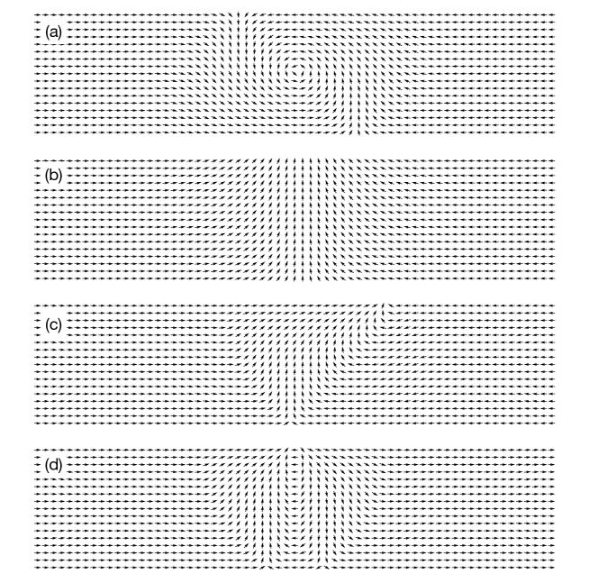
Figure 1. Domain wall profiles in the numerical simulations of amorphous cobalt nanostrips: (a) vortex head-to-head wall in a 100 nm wide and 5 nm thick strip; (b) symmetric transverse head-to-head wall in a 50 nm wide and 2 nm thick strip; (c) asymmetric head-to-head wall in a 400 nm wide and 5 nm thick strip; (d) a winding transverse domain wall in a 400 nm wide and 5 nm thick strip. The material parameters are: exchange constant $A=1.4\times 10^{-11}$ J/m, saturation magnetization $M_{s}=1.4\times 10^{6}$ A/m, and zero magnetocrystalline anisotropy or applied magnetic field [44]. For this material, the exchange length is $\ell_{\mathrm{ex}}=3.37$ nm.

The mathematical understanding of domain wall profiles in ferromagnets rests on the micromagnetic modeling framework, whereby the magnetization configurations representing these profiles are viewed as local or global minimizers of the micromagnetic energy functional [29, 42]. This framework has been successfully used to characterize a great variety of domain walls and other magnetization configurations (for an overview, see [15]; for some more recent developments, see [30, 12, 19, 31, 53, 47, 35, 46]). However, head-to-head domain walls pose a fundamental challenge to micromagnetic modeling and analysis, since these magnetization configurations carry a non-zero magnetic charge, which may lead to divergence of the wall energy in infinite samples due to singular behaviors of the stray field [47]. To date, there have been only a handful of micromagnetic studies of such charged domain walls [38, 39, 26, 27, 47, 46, 36].

In [38, 39], Kühn studied head-to-head domain walls in cylindrical nanowires of radius $R>0$. These walls are viewed as global minimizers of the energy

(1.1) $$\mathcal{E}(m):=\frac{1}{2}\int_{\Sigma}|\nabla m|^{2}d^{3}r+\frac{1}{2}\int_{\mathbb{R}^{3}}|\nabla u|^{2}d^{3}r,$$

where $m\in H^{1}_{loc}(\Sigma;\mathbb{S}^{2})$, $\Sigma=\Sigma_{R}:=\mathbb{R}\times B_{R}(0)\subset\mathbb{R}^{3}$, and $u\in\mathring{H}^{1}(\mathbb{R}^{3})$ is the magnetostatic potential solving

(1.2) $$\Delta u=\nabla\cdot m$$

distributionally in $\mathbb{R}^{3}$, with $m$ extended by zero to $\mathbb{R}^{3}\backslash\Sigma$. The magnetization $m$ is subject to the condition at infinity

(1.3) $$m(x,y,z)\to(\pm 1,0,0)\qquad\text{as}\qquad x\to\pm\infty,$$

in some average sense (for a recent discussion of variational principles of micromagnetics, see [16]). Kühn considered existence of minimizers of $\mathcal{E}$ in a suitable class of magnetizations $m$ for which (1.3) holds, as well as a number of their characteristics depending on $R$. In particular, she showed that as $R\to 0$ the domain wall profile is expected to converge, in an appropriate sense, to that of a one-dimensional transverse wall, which is given explicitly, up to translations along the $x$-axis and rotations in the $yz$-plane, by

(1.4) $$m(x,y,z)=\left(\tanh(x/\sqrt{2}),\text{sech}(x/\sqrt{2}),0\right).$$

Existence and convergence of minimizers were later established by Harutyunyan for general cylindrical domains $\Sigma=\mathbb{R}\times\Omega$, where $\Omega\subset\mathbb{R}^{2}$ is a bounded domain with a $C^{1}$ boundary [27] (see also [61]). In [26], Harutyunyan also studied the behavior of the limit energy when $\Omega$ is a rectangle with a large aspect ratio and obtained an additional logarithmic factor in the scaling of the optimal energy (for sharp asymptotics, see [22]).

In the case of $\Sigma=\Sigma_{R}$ with $R>0$ sufficiently small, the analysis mentioned above is enabled by the fact that as $R\to 0$ the magnetization becomes essentially constant in the $yz$-plane, allowing to asymptotically reduce the energy to $\mathcal{E}(m)\simeq\mathcal{E}_{0}^{\mathrm{1d}}(\bar{m})$, where $\bar{m}(x,y,z):=\displaystyle\lim_{R\to 0}\left({1\over\pi R^{2}}\int_{B_{R}(0)}m(x,y^{\prime},z^{\prime})\,dy^{\prime}dz^{\prime}\right)$ and

(1.5) $$\mathcal{E}_{0}^{\mathrm{1d}}(\bar{m}):=\int_{\Sigma_{R}}\left(\frac{1}{2}|\nabla\bar{m}|^{2}+\frac{1}{4}\left(1-\bar{m}_{1}^{2}\right)\right)d^{3}r,$$

whose minimizers among all $\bar{m}\in\mathring{H}^{1}(\Sigma_{R};\mathbb{S}^{2})$ with $\bar{m}=\bar{m}(x)$ satisfying (1.3) are given by (1.4), up to translations and rotations in the $yz$-plane. The latter follows from the fact that the limit energy $\mathcal{E}_{0}^{\mathrm{1d}}$ in (1.5) is fully local, and its minimizers satisfy a simple ordinary differential equation that can be solved explicitly. The situation becomes much more complicated for general values of $R\gtrsim 1$ or for general cross-sections $\Omega$, since in that case the Euler-Lagrange equation for the minimizers of $\mathcal{E}$ is a system of nonlinear partial differential equations whose explicit solution is no longer available. In particular, it is not known whether or not the minimizers could exhibit winding, whereby the magnetization rotates by an integer multiple of 360^∘ along the axis of the wire, as, e.g., in Fig. 1(d).

In the absence of exact solutions and in view of the interest from applications, one can alternatively focus on the case of asymptotically thin films, i.e., for $\delta\ll 1$ to consider the energy $\mathcal{E}_{\delta}(m)$ given by $\mathcal{E}(m)$ in (1.1), in which $\Sigma=\Sigma_{\delta}:=\mathbb{R}\times(0,\delta)\times(0,w_{\delta})$. Here $\delta>0$ is the film thickness and $w_{\delta}>0$ is the film width, respectively, both in the units of the exchange length, with the dependence of $w_{\delta}$ on $\delta$ as $\delta\to 0$ to be specified. Notice that if $\Sigma_{\delta}$ were a bounded domain with the lateral extent of order $w_{\delta}$, then from the results of Kohn and Slastikov [37] one could conclude that the full micromagnetic energy $\mathcal{E}$ asymptotically reduces to $\mathcal{E}(m)\simeq\mathcal{E}_{0}^{\mathrm{2d}}(\bar{m})$, where $\bar{m}(x,y,z):=\displaystyle\lim_{\delta\to 0}\left({1\over\delta}\int_{0}^{\delta}m(x,y,z^{\prime})\,dz^{\prime}\right)$ such that $\bar{m}_{3}=0$ and

(1.6) $$\mathcal{E}_{0}^{\mathrm{2d}}(\bar{m}):=\frac{1}{2}\int_{\Sigma_{\delta}}|\nabla\bar{m}|^{2}d^{3}r+{\gamma\over w_{\delta}}\int_{\Gamma_{\delta}}(\bar{m}\cdot\nu)^{2}d\mathcal{H}^{2},$$

where $\Gamma_{\delta}$ is the portion of the boundary of $\Sigma_{\delta}$ associated with the film edge and $\nu$ is the outward unit normal to $\Gamma_{\delta}$, provided

(1.7) $$w_{\delta}={4\pi\gamma\over\delta\ln\delta^{-1}},$$

for some $\gamma>0$ fixed, as $\delta\to 0$.

Rescaling all lengths in the film plane with $w_{\delta}$ and writing $\bar{m}=(\cos\theta,\sin\theta)$, we then formally have $\mathcal{E}(m)\simeq\mathcal{F}(\theta)\delta$, where

(1.8) $$\mathcal{F}(\theta):=\frac{1}{2}\int_{\Sigma_{0}}|\nabla\theta|^{2}d^{2}r+\gamma\int_{\partial\Sigma_{0}}\sin^{2}\theta\,d\mathcal{H}^{1},$$

$\Sigma_{0}:=\mathbb{R}\times(0,1)$ denotes an infinite strip of unit width, and $\theta\in C^{1}(\overline{\Sigma}_{0})$, for example. As expected, in this scaling regime the contribution of the stray field to the energy localizes to become a nonlinear boundary penalty term, greatly simplifying the otherwise highly nonlocal problem for the domain wall profiles.

Note, however, that finding the profile in this case does not reduce to solving an ordinary differential equation for the magnetization angle, as in the case of thin ferromagnetic wires discussed earlier. Instead, the problem may be reduced to a one-dimensional fractional differential equation. To see this, let us formally reduce the minimization problem for $\mathcal{F}$ to the problem for the trace of $\theta$ on $\partial\Sigma_{0}$ (for details, see Appendix A). It is easy to see that any minimizer of $\mathcal{F}$ in the form of a domain wall must be reflection-symmetric with respect to the midline of $\Sigma$. Hence for a given trace $\bar{\theta}\in C^{\infty}(\mathbb{R})$ of $\theta$ on $\partial\Sigma_{0}$ such that

(1.9) $$\bar{\theta}(x)=k_{1}\pi\quad\forall x<-R,\qquad\qquad\bar{\theta}(x)=k_{2}\pi\quad\forall x>R,$$

for some $R>0$ and $k_{1},k_{2}\in\mathbb{Z}$ we can minimize the Dirichlet integral by choosing $\theta$ to be the harmonic extension of $\bar{\theta}$. A direct computation then shows that $\mathcal{F}(\theta)=2\bar{\mathcal{F}}(\bar{\theta})$, where

(1.10) $$\bar{\mathcal{F}}(\bar{\theta}):=\frac{1}{4}\int_{\mathbb{R}}\int_{\mathbb{R}}K(x-x^{\prime})(\bar{\theta}(x)-\bar{\theta}(x^{\prime}))^{2}dx\,dx^{\prime}+\gamma\int_{\mathbb{R}}\sin^{2}\bar{\theta}(x)\,dx,$$

in which the symmetric, positive definite kernel

(1.11) $$K(x):={\pi\cosh(\pi x)\over\sinh^{2}(\pi x)}$$

has the same singularity at the origin as the kernel generating $(-d^{2}/dx^{2})^{1/2}$ [18] and decays exponentially at infinity.

The Euler-Lagrange equation corresponding to $\bar{\mathcal{F}}$ reads

(1.12) $$\frac{1}{2}\int_{\mathbb{R}}\big{(}2\bar{\theta}(x)-\bar{\theta}(x-\xi)-\bar{\theta}(x+\xi)\big{)}K(\xi)d\xi+\gamma\sin 2\bar{\theta}(x)=0\qquad\forall x\in\mathbb{R}.$$

This equation is reminiscent of the fractional Ginzburg-Landau equation studied in [10, 56, 11], which is known to exhibit transition layer profiles connecting the limits at infinity that differ by $\pm\pi$ corresponding to the adjacent minima of the wells of the potential appearing in the last term in (1.10). Contrary to the problem in [10, 56, 11], however, the infimum of the energy in (1.10) is finite, making it amenable to analysis via direct minimization. Note that when $\gamma\gg 1$, minimizers of $\bar{\mathcal{F}}$ are expected to concentrate on the $O(\gamma^{-1})$ length scale (for a closely related problem, see [41]). In this case one can approximate $K(x)\simeq{1\over\pi x^{2}}$, for which all domain wall type solutions of (1.12) are [65]

(1.13) $$\bar{\theta}(x)=\pm\arctan 2\gamma x+{\pi\over 2},$$

up to translations and additions of integer multiples of $\pi$. Thus, the head-to-head domain wall profiles minimizing $\mathcal{E}$ with $\Sigma=\mathbb{R}\times(0,\delta)\times(0,w_{\delta})$ in the regime of $\delta\ll 1$ and $w_{\delta}$ given by (1.7) with $\gamma\gg 1$ are expected to consist of magnetizations rotating in the film plane in the form of two symmetric boundary vortices on the opposite sides of the strip, consistently with the heuristics presented in [63]. Alternatively, when $\gamma\ll 1$, one would expect the minimizers of $\bar{\mathcal{F}}$ to vary on an $O(\gamma^{-1/2})$ scale, for which one can approximate $x^{2}K(x)\simeq\delta(x)$, where $\delta(x)$ is the Dirac delta-function (cf. also [8]). In this case (1.12) would reduce to an ordinary differential equation

(1.14) $${d^{2}\bar{\theta}(x)\over dx^{2}}=2\gamma\sin 2\bar{\theta}(x)\qquad\forall x\in\mathbb{R},$$

whose all domain wall type solutions are $\bar{\theta}(x)=\pm 2\,\arctan\left(e^{2\sqrt{\gamma}\,x}\right)$, up to translations and additions of integer multiples of $\pi$. After a suitable rescaling and a possible reflection, these correspond to the profile in (1.4).

The minimization of the energy (1.10) could in principle be carried out directly, yielding existence and properties of minimizers for (1.8). The situation becomes more complicated, however, in the presence of an applied external field $h>0$ along the strip, which amounts to an extra Zeeman term [29] added to the energy in (1.1):

(1.15) $$\mathcal{E}(m):=\frac{1}{2}\int_{\Sigma}|\nabla m|^{2}d^{3}r+h\int_{\Sigma}\left(1-m_{1}\right)d^{3}r+\frac{1}{2}\int_{\mathbb{R}^{3}}|\nabla u|^{2}d^{3}r,$$

after subtracting a suitable additive constant. At the level of the limit thin film energy in (1.8), this translates into

(1.16) $$\mathcal{F}(\theta):=\frac{1}{2}\int_{\Sigma_{0}}|\nabla\theta|^{2}d^{2}r+h\int_{\Sigma_{0}}(1-\cos\theta)\,d^{2}r+\gamma\int_{\partial\Sigma_{0}}\sin^{2}\theta\,d\mathcal{H}^{1},$$

and clearly one could no longer explicitly minimize the first two terms in the energy for a given trace $\bar{\theta}$, as this would involve solving a nonlinear partial differential equation for $\theta$ in $\Sigma_{0}$. Instead, we will work directly with the energy in (1.16) and study its minimizers for $h\geq 0$ that connect distinct equilibrium solutions $\theta=\mathrm{const}$ as $x\to\pm\infty$.

We first focus on (1.16) and establish existence of energy minimizers that connect distinct equilibria at $x=\pm\infty$, using the direct method of calculus of variations. The difficulty here is the fact that the problem is posed on an unbounded domain and, therefore, a priori minimizing sequences may fail to converge to a function that has the right behavior at infinity. We overcome this difficulty by proving monotonicity of the minimizers on larger and larger truncated domains with prescribed Dirichlet data at the left and the right ends of the truncated strip. Taking the limit of the sequence of truncated minimizers, after suitable translations, we obtain a limiting monotone function. Combining this fact with the knowledge of the behavior at infinity for functions with bounded energy (1.16) (see Lemma 3.1), we show that this limiting function is non-trivial and has the appropriate behavior at infinity. By lower semicontinuity of the energy, we subsequently conclude that the obtained limit is the desired minimizer.

Notice that the Euler-Lagrange equation form the energy in (1.16) is reminiscent of problems arising in the studies of front solutions in infinite cylinders, on which there exists an extensive literature. For example, when $\gamma=0$ and $h>0$ the existence and qualitative properties of such solutions were established in [7]. A novel aspect of the considered problem is the fact that the bistable nonlinearity enabling existence of the front solutions is concentrated on the domain boundary (for several studies of problems of this kind, see e.g. [10, 13, 4, 28]; this list is certainly not exhaustive). Our contribution here is to develop a set of tools to address the problems with boundary nonlinearities based on maximum and comparison principles and the sliding method. Using these tools, we completely classify the critical points corresponding to domain wall solutions and establish regularity, symmetry, uniqueness, monotonicity and decay properties of the domain wall profiles. In particular, we show that after reflections, translations and shifts in $\theta$, all domain wall solutions associated with (1.16) are the energy minimizers that connect two distinct equilibria at infinity with no winding for $h=0$ (symmetric $180^{\circ}$ walls) or the same equilibrium at infinity with exactly one rotation for $h>0$ (symmetric $360^{\circ}$ walls). We also establish the explicit limit behaviors of the minimizers in the limiting regimes of $\gamma\to 0$ and $\gamma\to\infty$ when $h=0$.

We finally relate the minimization problem associated with (1.16) with that of the original micromagnetic problem associated with (1.15). To this end, we introduce a reduced thin film micromagnetic energy functional that is appropriate for modeling ultrathin ferromagnetic films in which the ferromagnetic layer has thicknesses down to a few atomic layers and, strictly speaking, the macroscopic energy functional in (1.15) is no longer applicable. This two-dimensional reduced thin film energy functional retains the nonlocal character of the micromagnetic energy in (1.15) in the ultrathin film regime and was introduced by us earlier in the studies of exchange biased films [46]. It represents an intermediate level of modeling between the full three-dimensional micromagnetic energy in (1.15) and the two-dimensional thin film limit energy in (1.16). Notice that the latter formally coincides with the one identified by Kohn and Slastikov in their studies of thin film limits of ferromagnets of finite lateral extent [37]. However, their analysis is no longer applicable in our setting due to the loss of compactness associated with the unbounded domain occupied by the ferromagnet. For this reason, we had to develop a series of new tools to tackle these issues in order to be able to prove the $\Gamma$-convergence of the reduced thin film energy (to be introduced in the following section, see (2.10)) to the limit thin film energy in (1.16), together with compactness and convergence of the respective energy minimizers as the film thickness goes to zero. Importantly, we also prove that at small but finite film thickness the non-trivial energy minimizers of the reduced thin-film energy (2.10) remain close in a certain sense to the unique minimizers of the limit problem associated with (1.16). In particular, they exhibit the same head-to-head (for $h=0$) or winding (for $h>0$) behavior.

Our paper is organized as follows. In Sec. 2, we state precisely the variational problems to be analyzed and the main results of the paper. In particular, the basic existence and qualitative properties of the domain wall profiles for the limit thin film problem are presented in Theorem 2.3, a complete characterization of all domain wall profiles of the limit problem is given in Theorem 2.6, and convergence of the minimizers in the regimes of large and small values of $\gamma$ for $h=0$ is presented in Theorem 2.7. Finally, a characterization and the asymptotic behavior of minimizers of the reduced thin film energy as the film thickness vanishes is presented in Theorem 2.9. In Sec. 3, we present the treatment of the limit thin film energy, in which the existence result for the minimizers is given by Theorem 3.2 and the rest of the section is devoted to the proofs of Theorem 2.3, Theorem 2.6 and Theorem 2.7. We also characterize the infimum energy for the limit thin film energy in the classes of configurations with prescribed winding in Corollary 3.3. Finally, in Sec. 4 we prove a $\Gamma$-convergence result for the reduced micromagnetic thin film energy to the limit energy analyzed in Sec. 3 in Theorem 4.9, and then establish Theorem 2.9 via a sequence of corollaries.

Acknowledgements

The work of CBM was supported, in part, by NSF via grants DMS-1614948 and DMS-1908709. MN was supported by the PRIN Project 2019/24. MM and MN are members of the INDAM/GNAMPA. VS acknowledges support by Leverhulme grant RPG-2018-438 and would like to thank the Max Planck Institute for Mathematics in the Sciences in Leipzig for support and hospitality.

2. Statement of results

We now turn to the precise statements of the main results of our paper. We begin by simplifying some of the notation. For the limit thin film energy, we drop the subscript “0” from the definition of the two-dimensional strip domain and simply write $\Sigma:=\mathbb{R}\times(0,1)\subset\mathbb{R}^{2}$. By $\mathbf{r}=(x,y)\in\Sigma$ we denote a generic point in the strip, with $x\in\mathbb{R}$ and $y\in(0,1)$. On the strip $\Sigma$ we introduce a local space $H^{1}_{l}(\Sigma)$ consisting of functions whose restrictions to truncated strips $Q_{R}:=(-R,R)\times(0,1)$ belong to $H^{1}(Q_{R})$ for any $R>0$. We equip $H^{1}_{l}(\Sigma)$ with the notion of convergence corresponding to the $H^{1}(Q_{R})$ convergence of the restrictions to $Q_{R}$. This space plays the role of the local space $H^{1}_{loc}(\Sigma)$ that allows to make sense of the traces of functions on $\partial\Sigma$ in the $L^{2}_{loc}(\partial\Sigma)$ sense.

For $h\geq 0$, $\gamma>0$ and $\theta\in H^{1}_{l}(\Sigma)$ the thin film limit energy

(2.1) $$F(\theta):=\int_{\Sigma}\left(\frac{1}{2}|\nabla\theta|^{2}+h(1-\cos\theta)\right)\,d^{2}r+\gamma\int_{\partial\Sigma}\sin^{2}\theta\,d\mathcal{H}^{1}$$

defines a map $F:H^{1}_{l}(\Sigma)\to[0,+\infty]$, provided the last term in (2.1) is understood in the sense of trace. Notice that the Euler-Lagrange equation associated with (2.1) is

(2.2) $$\begin{cases}\Delta\theta=h\sin\theta&\text{in }\Sigma\,,\\ \partial_{\nu}\theta=-\gamma\sin(2\theta)&\text{on }\partial\Sigma\,,\end{cases}$$

where $\partial_{\nu}\theta$ denotes the derivative of $\theta$ in the direction of the outward normal $\nu$ to $\partial\Sigma$. The weak form of (2.2) is

(2.3) $$\int_{\Sigma}(\nabla\theta\cdot\nabla\varphi+h\sin(\theta)\,\varphi)\,d^{2}r+\gamma\int_{\partial\Sigma}\sin(2\theta)\,\varphi\,d\mathcal{H}^{1}=0\qquad\forall\varphi\in H^{1}_{l}({\Sigma})\text{ with bounded support}.$$

Remark 2.1.

By Lemma 3.4 below, any bounded weak solution to (2.2), i.e., any $\theta\in H^{1}_{l}(\Sigma){\cap L^{\infty}(\Sigma)}$ satisfying (2.3) belongs to $C^{\infty}(\overline{\Sigma})$ and thus is a classical solution of (2.2). Therefore, throughout the paper we will not distinguish between weak and strong formulations of the problem.

Next, for $k\in\mathbb{Z}$ we introduce a class of functions

(2.4) $$\mathcal{A}_{k}:=\Bigl{\{}\theta\in H^{1}_{l}(\Sigma):\,\lim_{x\to+\infty}\|\theta(x,\cdot)\|_{L^{2}(0,1)}=0,\lim_{x\to-\infty}\|\theta(x,\cdot)-k\pi\|_{L^{2}(0,1)}=0\Bigr{\}}\,,$$

where $\theta(x,\cdot)$ is understood as a trace. These functions correspond to the in-plane magnetization profiles $m=(\cos\theta,\sin\theta)$ connecting $\theta(x,y)=0$ at $x=+\infty$ with $\theta(x,y)=k\pi$ at $x=-\infty$ in an average sense. For the limit energy $F$, we are then interested in the following variational problem:

(2.5) $$\text{minimize}\ F(\theta)\ \text{over}\ \theta\in\mathcal{A}_{k}\ \text{with}\ k\not=0\ \text{fixed}.$$

Remark 2.2.

Note that if $\theta\in\mathcal{A}_{k}$, then $-\theta\in\mathcal{A}_{-k}$ with $F(\theta)=F(-\theta)$. In particular, for every $k\in\mathbb{N}$ we have

$$\inf_{\theta\in\mathcal{A}_{k}}F(\theta)=\inf_{\theta\in\mathcal{A}_{-k}}F(\theta)\,.$$

In view of the previous remark, we may restrict ourselves to the case $k\in\mathbb{N}$ in (2.5).

Our first result concerns existence, uniqueness and qualitative properties of the minimizers of $F$ in $\mathcal{A}_{k}$.

Theorem 2.3.

Let $\gamma>0$, $h\geq 0$ and $k\in\mathbb{N}$. Then a minimizer $\theta_{min}$ of $F$ over $\mathcal{A}_{k}$ exists if and only if $k=1$ for $h=0$, or if and only if $k=2$ for $h>0$. The minimizer is unique up to translations along the $x$ direction, belongs to $C^{\infty}(\overline{\Sigma})$ with derivatives of all orders bounded and satisfies (2.2) classically. In addition, for all $(x,y)\in\overline{\Sigma}$ the minimizer $\theta_{min}$ satisfies:

• (strict monotone decrease) $\partial_{x}\theta_{min}(x,y)<0$;

• (symmetry) $\theta_{min}(x,y)=\theta_{min}(x,1-y)$ and $\theta_{min}(x,y)=k\pi-\theta_{min}(a-x,y)$ for some $a\in\mathbb{R}$;

• (exponential decay at infinity) for every $m\in\mathbb{N}$ there exist positive constants $\alpha_{m}$, $\beta_{m}$ such that

  $$\|\theta_{min}-k\pi\|_{C^{m}((-\infty,-t]\times[0,1])}\leq\alpha_{m}\mathrm{e}^{-\beta_{m}t}\quad\text{and}\quad\|\theta_{min}\|_{C^{m}([t,+\infty)\times[0,1])}\leq\alpha_{m}\mathrm{e}^{-\beta_{m}t}$$

  for all $t>0$ sufficiently large.

Our next result characterizes all domain wall type solutions for the limit thin film model, i.e., all bounded solutions of (2.2) that attain distinct pointwise limits as $x\to\pm\infty$. More precisely, we introduce the following definition.

Definition 2.4.

Let $\theta\in C^{2}(\Sigma)\cap C^{1}(\overline{\Sigma})\cap L^{\infty}(\Sigma)$ be a solution of (2.2). We say that $\theta$ is a domain wall solution if there exist $\ell^{-},\ell^{+}\in\mathbb{R}$, $\ell^{-}>\ell^{+}$, such that

(2.6) $$\lim_{x\to-\infty}\theta(x,y)=\ell^{-}\quad\text{and}\quad\lim_{x\to+\infty}\theta(x,y)=\ell^{+}\qquad\text{ for all }y\in(0,1)\,.$$

Remark 2.5.

We make several observation regarding the above definition:

• The condition $\ell^{-}>\ell^{+}$ is assumed without loss of generality, as otherwise we can replace $\theta(x,y)$ with $\theta(-x,y)$ in all the statements.

• If $\theta$ is a domain wall solution in the sense of Definition 2.4 and $k$ any integer, then $\theta+2k\pi$ is a domain wall solution as well. If additionally $h=0$, so is also $\theta+k\pi$.

• By Lemma 3.4, any bounded weak solution (2.3) is smooth up to the boundary with derivatives of all orders bounded, and, therefore, it solves (2.2) classically. In particular, domain wall solutions in the sense of Definition 2.4 belong to $C^{\infty}(\overline{\Sigma})$, and their derivatives of all orders are bounded. Moreover, by the same lemma, the convergence to $\ell^{\pm}$ in (2.6) holds in fact in a much stronger sense, namely uniformly with respect to the $C^{m}$-norm, for every $m\in\mathbb{N}$, see (3.27).

• If $h=0$, or if $h>0$ and $F(\theta)<+\infty$, then condition (2.6) can be replaced (see Lemma 3.5) by the following one:

  (2.7) $$\lim_{x\to-\infty}\theta(x,0)=\lim_{x\to-\infty}\theta(x,1)=\ell^{-}\quad\text{and}\quad\lim_{x\to+\infty}\theta(x,0)=\lim_{x\to+\infty}\theta(x,1)=\ell^{+}\,.$$

We also note that in view of Remark 2.5-c) the functions $\theta(x,y)=\ell^{\pm}$ must themselves solve (2.2). Hence, a priori we should have $\ell^{\pm}\in{\pi\over 2}\mathbb{Z}$ when $h=0$ and $\ell^{\pm}\in\pi\mathbb{Z}$ when $h>0$.

We now state the theorem about domain wall type solutions. In essence, our next result shows that the only domain wall type critical points of $F$ are the minimizers obtained in Theorem 2.3, up to a reflection and an addition of a multiple of $\pi$.

Theorem 2.6.

Let $\gamma>0$ and $h\geq 0$, let $\theta$ be a domain wall solution in the sense of Definition 2.4, and let $\theta_{min}$ be as in Theorem 2.3. Then the following uniqueness properties hold true:

• If $h=0$, then there exist $k\in\mathbb{Z}$ and $\lambda\in\mathbb{R}$ such that $\ell^{+}=k\pi$, $\ell^{-}=(k+1)\pi$, and for every $(x,y)\in\overline{\Sigma}$

  $$\theta{(x,y)}=\theta_{min}({x+\lambda,y})+k\pi\,;$$

• If $h>0$, then there exist $k\in\mathbb{Z}$ and $\lambda\in\mathbb{R}$ such that $\ell^{+}=2k\pi$, $\ell^{-}=(2k+2)\pi$, and for every $(x,y)\in\overline{\Sigma}$

  $$\theta{(x,y)}=\theta_{min}({x+\lambda,y})+2k\pi\,.$$

Before turning to the relation between the thin limit model in (2.1) and the micromagnetic energy, we also consider the asymptotic behavior of the domain wall solutions for both $\gamma\ll 1$ and $\gamma\gg 1$. In view of Theorem 2.6, it is sufficient to consider the minimizers of $F$ in the appropriate function classes. For simplicity of presentation, we will only consider the most interesting case $h=0$, as the case $h>0$ may be treated analogously, albeit without an explicit limiting solution when $\gamma\to\infty$.

Theorem 2.7.

For $\gamma>0$ and $h=0$, let $\theta_{min,\gamma}$ be the unique minimizer of $F$ over $\mathcal{A}_{1}$ satisfying ${\theta_{min,\gamma}}(0,\cdot)={\pi\over 2}$. Then

• ${\theta_{min,\gamma}}(x/\sqrt{\gamma},y)\to\pi-2\arctan(e^{2x})$ as $\gamma\to 0$;

• ${\theta_{min,\gamma}}(x,y)\to{\pi\over 2}-\arctan\left({\sinh(\pi x)\over\sin(\pi y)}\right)$ as $\gamma\to\infty$,

locally uniformly in $\Sigma$.

Remark 2.8.

As may be seen from the proof, the result in part a) of Theorem 2.7 also holds with respect to the $H^{1}_{l}(\Sigma)$ convergence. However, the latter does not hold for part b), as the limit function fails to be in $H^{1}_{l}(\Sigma)$. Finally, in the case $h>0$ and $\gamma\to 0$ the limit solution is easily seen to be that of (2.2) with $\gamma=0$ and is, once again, one-dimensional, while as $\gamma\to\infty$ the solution is expected to converge to a solution of the first equation in (2.2) with Dirichlet boundary condition in the form of a piecewise-constant function taking values $0$ and $2\pi$.

Notice that the result in part b) of Theorem 2.7 provides a rigorous basis for the physical picture presented in [63]. Also, Theorem 2.7 provides a rigorous counterpart for the discussion in the introduction regarding the limiting behavior of the magnetization in the strip in the limits of large and small values of $\gamma$.

We finally turn to the relationship of the results obtained by us for the limit thin film energy in (2.1) with those for the micromagnetic energy. Notice that in the regime of interest the film thickness reaches an order of only a few atomic layers, making the use of the full three-dimensional micromagnetic energy problematic. As was argued previously, a model that is more appropriate for such ultrathin films is the reduced micromagnetic thin film energy (for a detailed discussion, see [46, 17]).

Let $d_{\Sigma}(\mathbf{r}):=\mathrm{dist}(\mathbf{r},\mathbb{R}^{2}\backslash\Sigma)$. For $\varepsilon>0$ sufficiently, small we consider the family of cutoff functions

(2.8) $$\eta_{\varepsilon}(\mathbf{r})=\eta\left(d_{\Sigma}(\mathbf{r})/\varepsilon\right),$$

where $\eta\in C^{1}([0,+\infty))$ is such that $\eta(0)=0$, $\eta^{\prime}(t)\geq 0$ for all $t\geq 0$ and $\eta(t)=1$ for $t\geq 1$. Then for

(2.9) $$m:\Sigma\to\mathbb{S}^{1},\quad m=(m_{1}(x,y),m_{2}(x,y)),$$

such that $m\in C^{\infty}(\overline{\Sigma};\mathbb{R}^{2})$ and $m_{2}$ vanishes outside a compact set, we define the following reduced micromagnetic energy:

(2.10) $$E_{\varepsilon}(m)=\frac{1}{2}\int_{\Sigma}|\nabla m|^{2}\,d^{2}r+\frac{\gamma}{2|\ln\varepsilon|}\int_{\Sigma}\int_{\Sigma}\frac{\textup{div}(\eta_{\varepsilon}m)(\mathbf{r})\,\textup{div}(\eta_{\varepsilon}m)(\mathbf{r}^{\prime})}{|\mathbf{r}-\mathbf{r}^{\prime}|}\,d^{2}r\,d^{2}r^{\prime}+h\int_{\Sigma}(1-m_{1})\,d^{2}r,$$

where $\gamma>0$ is a fixed parameter, which may be obtained from the full three-dimensional micromagnetics via a formal asymptotic reduction and a suitable rescaling of the strip width [46, 17]. The conditions on $m$, which we are going to relax shortly, are needed to ensure convergence of all the integrals in (2.10). In particular, it ensures that $m_{1}(x,y)=\pm 1$ for all $|x|$ large enough, corresponding to the head-to-head or winding domain wall configurations.

In (2.10), the parameter $\varepsilon$ represents the effective dimensionless film thickness measured relative to the strip width, and $\gamma$ is an effective stray field strength normalized by $|\ln\varepsilon|$ (compare with (1.6)). As was already mentioned, this energy is somewhat intermediate in the hierarchy of multiscale micromagnetic energies between the full three-dimensional micromagnetic energy in (1.1) (with the Zeeman term added) and the limit thin film energy in (2.1).

The assumptions about $m$ above are clearly too restrictive for the existence of unconstrained minimizers of $E_{\varepsilon}$. To find a more appropriate functional setting to seek the energy minimizers in the form of head-to-head or winding domain walls, we pass to the Fourier space in the nonlocal term and introduce the transform $\mathscr{F}(\mathrm{div}(\eta_{\varepsilon}m))$ of $\mathrm{div}(\eta_{\varepsilon}m)\in C^{\infty}_{c}(\mathbb{R}^{2})$:

(2.11) $$\mathscr{F}(\mathrm{div}(\eta_{\varepsilon}m))(k_{1},k_{2})=\int_{0}^{1}\int_{\mathbb{R}}e^{-ik_{1}x-ik_{2}y}\mathrm{div}(\eta_{\varepsilon}(y)m(x,y))\,dx\,dy,$$

where $\mathrm{div}(\eta_{\varepsilon}m)$ was extended by zero outside $\Sigma$. Clearly, under our assumption we have [45, Theorem 5.9]

(2.12) $$\int_{\Sigma}\int_{\Sigma}\frac{\textup{div}(\eta_{\varepsilon}m)(\mathbf{r})\,\textup{div}(\eta_{\varepsilon}m)(\mathbf{r}^{\prime})}{2\pi|\mathbf{r}-\mathbf{r}^{\prime}|}\,d^{2}r\,d^{2}r^{\prime}=\int_{\mathbb{R}^{2}}{|\mathscr{F}(\mathrm{div}(\eta_{\varepsilon}m))|^{2}\over|\mathbf{k}|}{d^{2}k\over(2\pi)^{2}},$$

which is nothing but the $\mathring{H}^{-1/2}(\mathbb{R}^{2})$ norm squared of $\textup{div}(\eta_{\varepsilon}m)$. Thus, under the above assumptions about $m$ the energy $E_{\varepsilon}(m)$ may be alternatively written in the form

(2.13) $$E_{\varepsilon}(m)=\frac{1}{2}\int_{\Sigma}|\nabla m|^{2}\,d^{2}r+\frac{\gamma}{2|\ln\varepsilon|}\int_{\mathbb{R}^{2}}{|\mathscr{F}(\textup{div}(\eta_{\varepsilon}m))|^{2}\over 2\pi|\mathbf{k}|}\,d^{2}k+h\int_{\Sigma}(1-m_{1})\,d^{2}r.$$

We now wish to relax the assumptions of smoothness of $m$ and of $m_{2}$ having compact support and introduce a more natural class of magnetizations for which the energy in (2.13) remains valid, taking advantage of positivity of the nonlocal energy term written in the Fourier space. Clearly, for $m\in H^{1}_{l}(\Sigma)$ all the local terms in the energy are well defined (possibly taking the value $+\infty$). It remains to make sense of the nonlocal term. For that purpose, observe that for $m\in H^{1}_{l}(\Sigma)$ we have (with a slight abuse of notation)

(2.14) $$\textup{div}(\eta_{\varepsilon}m)(x,y)=\eta_{\varepsilon}(y)\partial_{x}m_{1}(x,y)+\eta_{\varepsilon}(y)\partial_{y}m_{2}(x,y)+\eta_{\varepsilon}^{\prime}(y)m_{2}(x,y)$$

distributionally. Therefore, under a natural condition that $\nabla m\in L^{2}(\Sigma;\mathbb{R}^{2})$ the first two terms in the right-hand side of (2.14), extended by zero outside $\Sigma$, belong to $L^{2}(\mathbb{R}^{2})$ and thus have a well-defined Fourier transform in the $L^{2}$-sense. To make sense of the third term, we additionally assume that $m_{2}\in L^{2}(\Sigma)$. Thus, we introduce the class

(2.15) $$\mathfrak{M}:=\left\{m\in H^{1}_{l}(\Sigma;\mathbb{S}^{1})\,:\,\nabla m\in L^{2}(\Sigma;\mathbb{R}^{2}),\,m_{2}\in L^{2}(\Sigma)\right\},$$

on which $E_{\varepsilon}:\mathfrak{M}\to[0,+\infty]$ is now well defined for all $\varepsilon\in(0,\frac{1}{2})$. Note that the assumption $m_{2}\in L^{2}(\Sigma)$ for all $m\in\mathfrak{M}$ forces $m_{1}(x,\cdot)$ to approach $\pm 1$ in some average sense as $x\to\pm\infty$, thus selecting the magnetization profiles in the form of head-to-head or winding walls.

We will show the $\Gamma$-convergence as $\varepsilon\to 0$ of the energy $E_{\varepsilon}$ defined on $\mathfrak{M}$ to the following reduced energy (see Sec. 4):

(2.16) $$E_{0}(m)=\frac{1}{2}\int_{\Sigma}|\nabla m|^{2}\,d^{2}r+h\int_{\Sigma}(1-m_{1})\,d^{2}r+\gamma\int_{\partial\Sigma}m^{2}_{2}\,d\mathcal{H}^{1}.$$

With a slight abuse of notation, when talking about the limit $\varepsilon\to 0$ we will always imply taking a sequence of $\varepsilon_{k}\to 0$ as $k\to\infty$.

Associated with the energy in (2.16), we have the following minimization problem:

(2.17) $$\text{minimize}\ E_{0}(m)\ \text{among}\\ \ m=(\cos\theta,\sin\theta)\in H^{1}_{l}(\Sigma;\mathbb{S}^{1})\text{ with }\theta\text{ satisfying \eqref{lemma1} for some }k_{1},\,k_{2}\in\mathbb{Z},\,k_{1}\neq k_{2}.$$

Notice that for $m=(\cos\theta,\sin\theta)$, this energy coincides precisely with that in (2.1), and such a lifting is always possible for any $m\in H^{1}_{l}(\Sigma;\mathbb{S}^{1})$ (see, for instance, [9]), making the energies $E_{0}(m)$ and $F(\theta)$ equivalent. The $\Gamma$-convergence result, stated in Theorem 4.9, is with respect to the strong $L^{2}_{loc}(\Sigma)$ convergence of maps $m_{\varepsilon}:\Sigma\to\mathbb{S}^{1}$. Using this $\Gamma$-convergence result, we can then establish existence and a characterization of the minimizers of $E_{\varepsilon}$ in the form of domain walls in terms of those of $E_{0}$ for all small enough $\varepsilon$. Note that the existence and properties of the latter are established by Theorem 2.3. Also note that by Theorem 2.3 the minimizers of $E_{0}$ over $H^{1}_{l}(\Sigma;\mathbb{S}^{1})$ with suitable behaviors at infinity belong to $\mathfrak{M}$.

Theorem 2.9.

Let $\gamma>0$, $h\geq 0$ and $k\in\mathbb{N}$. Then there exists $\varepsilon_{0}>0$ such that for all $\varepsilon\in(0,\varepsilon_{0})$ there exists a minimizer $m=(\cos\theta,\sin\theta)$ of $E_{\varepsilon}$ over all $m\in\mathfrak{M}$ with $\theta\in\mathcal{A}_{k}$ if and only if $k=1$ when $h=0$, or if and only if $k=2$ when $h>0$. As $\varepsilon\to 0$, every minimizer of $E_{\varepsilon}$ above converges in $H^{1}_{l}(\Sigma;\mathbb{R}^{2})$, after a suitable translation, to the corresponding minimizer of $E_{0}$.

The above result shows that, in the considered regime of ultrathin ferromagnetic films, the domain wall-like ground states of the micromagnetic energy are head-to-head walls with no winding ($180^{\circ}$ walls) in the absence of the applied field ($h=0$). When an applied field is present ($h>0$), the only domain wall-like ground states are winding domain walls with a single rotation ($360^{\circ}$ walls). Furthermore, as the film thickness tends to zero these ground state profiles converge to the uniquely defined energy minimizing profiles for the limit energy $E_{0}$ (up to translations). Thus, in particular our results provide a mathematical understanding for the symmetric head-to-head domain wall profiles in the absence of the applied field observed in experiments and numerical simulations of sufficiently thin nanostrips (see Fig. 1(b)) and the discussion in Sec. 1. At the same time, our analysis does not capture the asymmetric head-to-head walls observed in wider nanostrips (see Fig. 1(c)). The analysis of the latter would require to consider a regime in which the stray field effect does not reduce to a purely local penalty term at the sample boundary, and is outside the regime studied in this paper. Similarly, our regime excludes the appearance of the vortex walls shown in Fig. 1(a).

3. Analysis of the thin film limit model

We start by recalling that for every $m\in H^{1}_{l}(\Sigma;\mathbb{S}^{1})$ there exists $\theta\in H^{1}_{l}(\Sigma)$ such that $m=(\cos\theta,\sin\theta)$ (see, for instance, [9]), and the energy (2.16) may be rewritten as

(3.1) $$E_{0}(m)=F(\theta).$$

In what follows, we identify any $\theta\in H^{1}_{l}(\Sigma)$ with the precise representative such that for every $x_{0}\in\mathbb{R}$, $\theta(x_{0},\cdot)$ coincides a.e. with the trace of $\theta$ on the vertical line $x=x_{0}$.

Lemma 3.1.

Let $\theta\in H^{1}_{l}(\Sigma)$ be such that $F(\theta)<+\infty$. Then there exist $k_{1},k_{2}\in\mathbb{Z}$ such that

(3.2) $$\lim_{x\to-\infty}\|\theta(x,\cdot)-k_{1}\pi\|_{L^{2}(0,1)}=0\text{ and }\lim_{x\to+\infty}\|\theta(x,\cdot)-k_{2}\pi\|_{L^{2}(0,1)}=0\,.$$

Furthermore, if $h>0$ we have $k_{1},k_{2}\in 2\mathbb{Z}$.

Proof.

Set

$$\bar{\theta}(x):=\int_{0}^{1}\theta(x,y)\,dy\,.$$

and note that $\bar{\theta}\in H^{1}_{loc}(\mathbb{R})$ and thus, in particular, it is continuous. We claim that

(3.3) $$\frac{1}{2}\int_{\mathbb{R}}|\bar{\theta}^{\prime}(x)|^{2}\,dx+2\gamma\int_{\mathbb{R}}\sin^{2}\bar{\theta}(x)\,dx\leq(5+8\gamma)F(\theta)\,.$$

We start by observing that

$$2\gamma\int_{\mathbb{R}}\sin^{2}\bar{\theta}(x)\,dx =2\gamma\int_{\mathbb{R}}\sin^{2}\theta(x,0)\,dx+2\gamma\int_{\mathbb{R}}(\sin^{2}\bar{\theta}(x)-\sin^{2}\theta(x,0))\,dx$$

$$\leq 4\gamma\int_{\mathbb{R}}\sin^{2}\theta(x,0)\,dx+4\gamma\int_{\mathbb{R}}|\sin\bar{\theta}(x)-\sin\theta(x,0)|^{2}\,dx$$

$$\leq 4\gamma\int_{\mathbb{R}}\sin^{2}\theta(x,0)\,dx+4\gamma\int_{\mathbb{R}}|\bar{\theta}(x)-\theta(x,0)|^{2}\,dx$$

$$\leq 4\gamma\int_{\mathbb{R}}\sin^{2}\theta(x,0)\,dx+4\gamma\int_{\mathbb{R}}\int_{0}^{1}|\partial_{y}\theta(x,y)|^{2}\,dy\,dx\leq(4+8\gamma)F(\theta)\,.$$

Equation (3.3) then follows.

Note that for every $\alpha<\beta$ we have

(3.4) $$\frac{1}{2}\int_{\alpha}^{\beta}|\bar{\theta}^{\prime}|^{2}\,dx+2\gamma\int_{\alpha}^{\beta}\sin^{2}\bar{\theta}\,dx\geq 2\sqrt{\gamma}\int_{\alpha}^{\beta}|\sin\bar{\theta}||\bar{\theta}^{\prime}|\,dx\geq 2\sqrt{\gamma}\big{|}\cos(\bar{\theta}(\beta))-\cos(\bar{\theta}(\alpha))\big{|}\,.$$

In particular, recalling (3.3), $\cos\bar{\theta}$ satisfies the Cauchy condition for $x\to+\infty$, that is

$$\lim_{\alpha,\beta\to+\infty}\big{|}\cos(\bar{\theta}(\beta))-\cos(\bar{\theta}(\alpha))\big{|}=0\,,$$

and thus $\cos\bar{\theta}$, and in turn $\sin^{2}\bar{\theta}$, admit a limit as $x\to+\infty$. Clearly the same is true for $x\to-\infty$.

Recalling (3.3), we conclude that

(3.5) $$\sin\bar{\theta}(x)\to 0\text{ and }\cos^{2}\bar{\theta}(x)\to 1\text{ as }|x|\to+\infty\,.$$

We now claim that there exist $k_{1},k_{2}\in\mathbb{Z}$ such that

(3.6) $$\lim_{x\to-\infty}\bar{\theta}(x)=k_{1}\pi\text{ and }\lim_{x\to+\infty}\bar{\theta}(x)=k_{2}\pi\,.$$

Let us show only the second limit. We argue by contradiction assuming that there exist two sequences $x_{n}<x^{\prime}_{n}$ both diverging to $+\infty$ such that $\liminf_{n\to\infty}|\bar{\theta}(x_{n})-\bar{\theta}(x^{\prime}_{n})|\geq\pi$. But then, by the continuity of $\bar{\theta}$ it is clear that we may also find $x^{\prime\prime}_{n}\in(x_{n},x^{\prime}_{n})$ such that $\cos^{2}\bar{\theta}(x^{\prime\prime}_{n})\to 0$, which contradicts (3.5). Thus, (3.6) holds.

Denote $Q^{t}:=(t-\frac{1}{2},t+\frac{1}{2})\times(0,1)$ and note that $\lim_{t\to\pm\infty}\|\nabla\theta\|_{L^{2}(Q^{t})}=0$. In turn, by a Poincaré-type inequality we have

$$\|\theta-\bar{\theta}(t)\|^{2}_{H^{1}(Q^{t})}\leq C\|\nabla\theta\|^{2}_{L^{2}(Q^{t})}$$

and thus, taking into account (3.6) we conclude that

$$\lim_{t\to+\infty}\|\theta-k_{2}\pi\|^{2}_{H^{1}(Q^{t})}=0\text{ and }\lim_{t\to-\infty}\|\theta-k_{1}\pi\|^{2}_{H^{1}(Q^{t})}=0\,.$$

By an application of the Trace Theorem we obtain (3.2). If $h>0$, then the fact that

$$\int_{\Sigma}(1-\cos\theta)\,dx<+\infty$$

implies that $k_{1}$, $k_{2}\in 2\mathbb{Z}$. ∎

Note that given $m\in H^{1}_{l}(\Sigma;\mathbb{S}^{1})$, the corresponding phase function $\theta$ is determined up to an additive constant of the form $k\pi$, where $k\in\mathbb{Z}$ if $h=0$ or $k\in 2\mathbb{Z}$ if $h>0$. In view of Lemma 3.1 we may additionally require that

(3.7) $$\lim_{x\to+\infty}\|\theta(x,\cdot)\|_{L^{2}(0,1)}=0\,.$$

Clearly by enforcing such a condition the phase function $\theta$ is uniquely determined.

In the next two subsections we address the existence of minimizers and the classification of domain wall solutions in the sense of Definition 2.4, respectively.

3.1. Existence of minimizers

We prove the following existence result.

Theorem 3.2.

If $h=0$ then the minimization problem (2.5) admits a solution for $k=1$. If $h>0$ then the minimization problem (2.5) admits a solution for $k=2$. In both cases, a solution $\theta_{min}$ can be found satisfying $\displaystyle\int_{0}^{1}\theta_{min}(0,y)\,dy=\frac{k\pi}{2}$. Moreover, $\theta_{min}\in C^{\infty}(\overline{\Sigma})$, with derivatives of all order bounded, and $\partial_{x}\theta_{min}<0$ in $\overline{\Sigma}$.

Proof.

We provide the proof only in the case $h>0$, as the case $h=0$ can be treated analogously and is simpler. To this end, for $M>0$ let

$$\mathcal{A}_{2,M}:=\big{\{}\theta\in\mathcal{A}_{2}:\,\theta=0\text{ in }\{(x,y)\in\Sigma:\,x\geq M\}\text{ and }\theta=2\pi\text{ in }\{(x,y)\in\Sigma:\,x\leq-M\}\big{\}},$$

and note that by standard arguments there exists a minimizer $\theta_{M}$ of $F$ over $\mathcal{A}_{2,M}$. Throughout the proof for every $M>0$ we set $\mathcal{R}_{M}:=(-M,M)\times(0,1)$.

We claim that

(3.8) $$\theta_{M}(x,y)\in(0,2\pi)\quad\text{ for all }(x,y)\in\mathcal{R}_{M}\,.$$

This follows by first observing that by an easy truncation procedure we may conclude that $\theta_{M}$ satisfies

(3.9) $$0\leq\theta_{M}\leq 2\pi\,.$$

Moreover, by a standard first variation argument $\theta_{M}$ is a weak solution to the following Euler-Lagrange problem

(3.10) $$\begin{cases}\Delta\theta_{M}=h\sin\theta_{M}&\text{in }\mathcal{R}_{M}\,,\\ \partial_{\nu}\theta_{M}=-\gamma\sin(2\theta_{M})&\text{on }\partial\mathcal{R}_{M}\cap\partial\Sigma\,,\\ \theta_{M}=0&\text{on }\{M\}\times(0,1)\,,\\ \theta_{M}=2\pi&\text{on }\{-M\}\times(0,1)\,,\end{cases}$$

that is,

(3.11) $$\int_{\mathcal{R}_{M}}(\nabla\theta_{M}\cdot\nabla\varphi+h\sin(\theta_{M})\,\varphi)\,d^{2}r+\gamma\int_{\partial\mathcal{R}_{M}\cap\partial\Sigma}\sin(2\theta_{M})\varphi\,d\mathcal{H}^{1}=0$$

for all $\varphi\in H^{1}(\mathcal{R}_{M})$ s.t. $\varphi=0$ on $\{-M,M\}\times(0,1)$.

Consider now the reflected function $\widetilde{\theta}_{M}$ defined on $\mathcal{R}_{3M}$ by

$$\widetilde{\theta}_{M}(x,y):=\begin{cases}-\theta_{M}(-x-2M,y)+4\pi&\text{if }x{\in(-3M,-M)},\\ \theta_{M}(x,y)&\text{if }x\in(-M,M)\,,\\ -\theta_{M}(-x+2M,y)&\text{if }x{\in(M,3M)}\,.\end{cases}$$

Using the weak formulation (3.11), one can immediately check that $\widetilde{\theta}_{M}$ is in turn a weak solution; that is,

$$\int_{\mathcal{R}_{3M}}(\nabla\widetilde{\theta}_{M}\cdot\nabla\varphi+h\sin(\widetilde{\theta}_{M})\,\varphi)\,d^{2}r+\gamma\int_{\partial\mathcal{R}_{3M}\cap\partial\Sigma}\sin(2\widetilde{\theta}_{M})\varphi\,d\mathcal{H}^{1}=0$$

for all $\varphi\in H^{1}(\mathcal{R}_{3M})$ s.t. $\varphi=0$ on $\{-3M,3M\}\times(0,1)$. We may then apply the very same arguments of Lemma 3.4-a) below (clearly, we can, since the regularity argument is local) to conclude that for every $0<M^{\prime}<3M$, $\widetilde{\theta}_{M}\in C^{\infty}(\overline{\mathcal{R}_{M^{\prime}}})$. In particular, $\theta_{M}\in C^{\infty}(\overline{\mathcal{R}_{M}})$, and (3.10) holds classically.

Note that we can write

$$\begin{cases}\Delta\theta_{M}=c(x,y)\theta_{M}&\text{in $(-M,M)\times(0,1)$,}\\ \partial_{\nu}\theta_{M}=-\gamma\sin(2\theta_{M})&\text{on }(-M,M)\times\{0,1\},\end{cases}$$

where we set

$$c(x,y):=\begin{cases}h\frac{\sin\theta_{M}(x,y)}{\theta_{M}(x,y)}&\text{if }\theta_{M}(x,y)>0\,,\\ h&\text{if }\theta_{M}(x,y)=0\,.\end{cases}$$

In order to prove (3.8), recall (3.9) and assume by contradiction that $\theta_{M}=0$ at some point in $(-M,M)\times(0,1)$. But then the Strong Maximum Principle [58, Theorem 2.2] applies and yields that $\theta_{M}\equiv 0$ in $(-M,M)\times(0,1)$, a contradiction to the fact that $\theta_{M}\in\mathcal{A}_{2,M}$. If instead $\theta_{M}=0$ at some point of the horizontal boundary $(-M,M)\times\{0,1\}$, then thanks to the Neumann condition in (3.10) also $\partial_{\nu}\theta_{M}$ vanishes at the same point and thus the contradiction follows from Hopf’s Lemma [23, Lemma 3.4]. Hence, we have shown that $\theta_{M}>0$ in $(-M,M)\times[0,1]$. Replacing $\theta_{M}$ by $2\pi-\theta_{M}$ and arguing as before, we complete the proof of (3.8).

We now show that $\theta_{M}$ is monotone non-increasing in the $x$-direction. To this aim, we adapt the classical sliding method of Berestycki and Nirenberg [6] (see also [7]) to the problem on the strip with nonlinear boundary conditions. Set

$$\bar{\lambda}:=\inf\{\lambda>0:\,\theta_{M}(\cdot+\mu,\cdot)\leq\theta_{M}\text{ in $\Sigma$ for all }\mu\geq\lambda\},$$

and observe that necessarily $\bar{\lambda}\in[0,2M)$. Indeed, clearly $\theta_{M}(\cdot+\mu,\cdot)\leq\theta_{M}$ for all $\mu\geq 2M$. Moreover, since $\theta_{M}(\cdot+2M,\cdot)=0<2\pi=\theta_{M}$ on $\{-M\}\times[0,1]$, by continuity we may find $\varepsilon>0$ so small that $\theta_{M}(\cdot+2M-s,\cdot)<\theta_{M}$ on $[-M,-M+s]\times[0,1]$ for all $s\in(0,\varepsilon]$, which in turn easily implies $\theta_{M}(\cdot+2M-s,\cdot)\leq\theta_{M}$ for the same $s$. Thus $\bar{\lambda}\leq 2M-\varepsilon$.

Note that $\bar{\lambda}=0$ if and only if $\theta_{M}$ is monotone non-increasing in the $x$-direction. Assume by contradiction that $\bar{\lambda}>0$. This means that $\theta_{M}(\cdot+\bar{\lambda},\cdot)\leq\theta_{M}$ and we claim that there exists $(\bar{x},\bar{y})\in[-M,M-\bar{\lambda}]\times[0,1]$ such that $\theta_{M}(\bar{x}+\bar{\lambda},\bar{y})=\theta_{M}(\bar{x},\bar{y})$. Indeed, if not then we would have $\theta_{M}(\cdot+\bar{\lambda},\cdot)<\theta_{M}$ in $[-M,M-\bar{\lambda}]\times[0,1]$ and in turn, arguing as above, $\theta_{M}(\cdot+\bar{\lambda}-\varepsilon,\cdot)\leq\theta_{M}$ in $[-M,M-\bar{\lambda}+\varepsilon]\times[0,1]$ for all $\varepsilon$ small enough, contradicting the minimality of $\bar{\lambda}$. We claim now that $\bar{x}\in({-M},M-\bar{\lambda})$. Indeed, if $\bar{x}=-M$, then $\theta_{M}(\bar{x}+\bar{\lambda},\bar{y})=\theta_{M}(\bar{x},\bar{y})=2\pi$ which is impossible thanks to (3.8) since $\bar{x}+\bar{\lambda}\in(-M,M)$. If instead $\bar{x}=M-\bar{\lambda}$, then $\theta_{M}(\bar{x},\bar{y})=\theta_{M}(M,\bar{y})=0$, which is again impossible by (3.8) since $\bar{x}<M$.

We now set $u:=\theta_{M}-\theta_{M}(\cdot+\bar{\lambda},\cdot)$. Note that $u$ satisfies

(3.12) $$\begin{cases}\Delta u=\tilde{c}u&\text{in }(-M,M-\bar{\lambda})\times(0,1)\,,\\ \partial_{\nu}u=-\gamma(\sin(2\theta_{M})-\sin(2\theta_{M}(\cdot+\bar{\lambda},\cdot)))&\text{on }(-M,M-\bar{\lambda})\times\{0,1\}\,,\\ u\geq 0\,,\\ u(\bar{x},\bar{y})=0\,,\end{cases}$$

where

$$\tilde{c}:=\begin{cases}h\frac{\sin(\theta_{M})-\sin(\theta_{M}(\cdot+\bar{\lambda},\cdot))}{\theta_{M}-\theta_{M}(\cdot+\bar{\lambda},\cdot)}&\text{in }\{\theta_{M}>\theta_{M}(\cdot+\bar{\lambda},\cdot)\}\,,\\ h&\text{in }\{\theta_{M}=\theta_{M}(\cdot+\bar{\lambda},\cdot)\}\,.\end{cases}$$

Now if $\bar{y}\in(0,1)$, then we can invoke again the Strong Maximum Principle [58, Theorem 2.2] to conclude that $u\equiv 0$ in $[-M,M-\bar{\lambda}]\times[0,1]$, and in particular that $\theta_{M}(M-\bar{\lambda},y)=\theta_{M}(M,y)=0$, which is a contradiction to (3.8). If instead $\bar{y}\in\{0,1\}$, then by Hopf’s Lemma [23, Lemma 3.4] we have $\partial_{\nu}u(\bar{x},\bar{y})\neq 0$, which contradicts the boundary condition in (3.12). This concludes the proof of the fact that $\bar{\lambda}=0$ and thus that $\theta_{M}$ is monotone non-increasing in the $x$-direction.

We now set $\bar{\theta}_{M}(x):=\int_{0}^{1}\theta_{M}(x,y)\,dy$. Note that $\bar{\theta}_{M}$ is continuous on $\mathbb{R}$ and that $\bar{\theta}_{M}(x)=0$ for $x\geq M$ and $\bar{\theta}_{M}(x)=2\pi$ for $x\leq-M$. Thus, we may find $x_{M}$ such that $\bar{\theta}_{M}(x_{M})=\pi$. We set $\tilde{\theta}_{M}:=\theta_{M}(\cdot+x_{M},\cdot)$. Observing that $F(\theta_{M})$ is non-increasing in $M$, we easily see that $\{\tilde{\theta}_{M}\}_{M\geq 1}$ is equibounded in $H^{1}_{l}(\Sigma)$. Thus, we may find a sequence $M_{n}\to+\infty$ and a function $\theta_{\infty}\in H^{1}_{l}(\Sigma)$ such that $\tilde{\theta}_{M_{n}}\rightharpoonup\theta_{\infty}$ weakly in $H^{1}_{l}(\Sigma)$, and

(3.13) $$F(\theta_{\infty})\leq\liminf_{n}F(\tilde{\theta}_{M_{n}})<+\infty\,.$$

Moreover, $0\leq\theta_{\infty}\leq 2\pi$, $\theta_{\infty}$ is monotone non-increasing in the $x$-direction, satisfies

(3.14) $$\int_{0}^{1}\theta_{\infty}(0,y)\,dy=\pi$$

and

(3.15) $$\begin{cases}\Delta\theta_{\infty}=h\sin\theta_{\infty}&\text{in }\Sigma\,,\\ \partial_{\nu}\theta_{\infty}=-\gamma\sin(2\theta_{\infty})&\text{on }\partial\Sigma\,.\end{cases}$$

in the weak sense. Again by Lemma 3.4, $\theta_{\infty}\in C^{\infty}(\overline{\Sigma})$, with derivatives of all orders bounded, and thus it satisfies (3.15) classically.

We claim that $\theta_{\infty}\in\mathcal{A}_{2}$. To this aim, in view of (3.13) and Lemma 3.1, and recalling that $0\leq\theta_{\infty}\leq 2\pi$, we have

$$\lim_{x\to-\infty}\|\theta_{\infty}(x,\cdot)-k_{1}\pi\|_{L^{2}(0,1)}=0\text{ and }\lim_{x\to+\infty}\|\theta_{\infty}(x,\cdot)-k_{2}\pi\|_{L^{2}(0,1)}=0\,,$$

with $k_{1},k_{2}\in\{0,2\}$. Now, by monotonicity and (3.14) we infer that necessarily $k_{1}=2$ and $k_{2}=0$. This shows that $\theta_{\infty}\in\mathcal{A}_{2}$.

In order to conclude that $\theta_{\infty}$ is a minimizer, in view of (3.13) it remains to show that

(3.16) $$\liminf_{n\to\infty}F(\tilde{\theta}_{M_{n}})=\inf_{\mathcal{A}_{2}}F\,.$$

To this aim, it is clearly enough to show that

(3.17) for $$\theta\in\mathcal{A}_{2} F(\theta)<+\infty \varepsilon>0 M>0 \tilde{\theta}\in\mathcal{A}_{2,M} F(\tilde{\theta})\leq F(\theta)+\varepsilon$$ with and there exists and such that .

In order to show this, we select two sequences, $x_{n}^{+}\to+\infty$ and $x_{n}^{-}\to-\infty$, such that

(3.18) $$\theta(x_{n}^{+},\cdot)\to 0\quad\text{and}\quad\theta(x_{n}^{-},\cdot)\to 2\pi\qquad\text{uniformly in }[0,1]\,,$$

and

(3.19) $$\limsup_{n\to\infty}\|\theta(x_{n}^{\pm},\cdot)\|_{H^{1}(0,1)}<+\infty\,.$$

This is possible by a simple slicing argument thanks to the fact that $|\nabla\theta|\in L^{2}(\Sigma)$. At this point, for every $n\in\mathbb{N}$ we define

$$\theta_{n}(x,y):=\begin{cases}\theta(x,y)&\text{if }x\in(x_{n}^{-},x_{n}^{+})\,,\\ \theta(x^{+}_{n},y)\left[\left(1-\frac{x-x_{n}^{+}}{\|\theta(x_{n}^{+},\cdot)\|_{\infty}}\right)\lor 0\right]&\text{if }x\geq x^{+}_{n}\,,\\ 2\pi-(2\pi-\theta(x_{n}^{-},y))\left[\left(1-\frac{x_{n}^{-}-x}{\|2\pi-\theta(x_{n}^{-},\cdot)\|_{\infty}}\right)\lor 0\right]&\text{if }x\leq x^{-}_{n}\,,\end{cases}$$

with the understanding that $\theta_{n}\equiv 0$ for $x\geq x_{n}$ if $\|\theta(x_{n}^{+},\cdot)\|_{\infty}=0$, and $\theta_{n}\equiv 2\pi$ for $x\leq x_{n}$ if $\|2\pi-\theta(x_{n}^{-},\cdot)\|_{\infty}=0$. Clearly each $\theta_{n}$ belongs to $\mathcal{A}_{2,M_{n}}$ for some $M_{n}>0$ sufficiently large. Moreover, using (3.18) and (3.19), it is easy to check that $F(\theta_{n})-F(\theta)\to 0$ as $n\to\infty$, thus establishing (3.17) and finishing the proof of existence.

We are left with showing that $\partial_{x}\theta_{\infty}<0$ in $\overline{\Sigma}$. We already know that $\theta_{\infty}$ is a smooth function, with $\partial_{x}\theta_{\infty}\leq 0$ everywhere. Differentiating (3.15) with respect to $x$ we obtain

(3.20) $$\begin{cases}\Delta(\partial_{x}\theta_{\infty})=h\cos\theta_{\infty}\partial_{x}\theta_{\infty}&\text{in }\Sigma\,,\\ \partial_{\nu}(\partial_{x}\theta_{\infty})=-2\gamma\cos(2\theta_{\infty})\partial_{x}\theta_{\infty}&\text{on }\partial\Sigma\,.\end{cases}$$

Assume $\partial_{x}\theta_{\infty}(\bar{x},\bar{y})=0$ at some point $(\bar{x},\bar{y})\in\overline{\Sigma}$. If $(\bar{x},\bar{y})\in\Sigma$, then using the Strong Maximum Principle [58, Theorem 2.2] we obtain a contradiction. If instead $(\bar{x},\bar{y})\in\partial\Sigma$, then also $\partial_{\nu}(\partial_{x}\theta_{\infty})$ vanishes at the same point and thus the contradiction follows from Hopf’s Lemma [23, Lemma 3.4]. ∎

Corollary 3.3.

If $h>0$ then for every $k\in 2\mathbb{N}$ we have

$$\inf_{\theta\in\mathcal{A}_{k}}F(\theta)=\frac{k}{2}\min_{\theta\in\mathcal{A}_{2}}F(\theta).$$

If $h=0$ then for every $k\in\mathbb{N}$ we have

$$\inf_{\theta\in\mathcal{A}_{k}}F(\theta)=k\min_{\theta\in\mathcal{A}_{1}}F(\theta).$$

Proof.

We provide the proof only for the case $h>0$, the other one being analogous. As in the previous proof, we fix $M>0$ and let

$$\mathcal{A}_{k,M}:=\{\theta\in\mathcal{A}_{k}:\,\theta(x,y)=0\text{ if }x\geq M\text{ and }\theta(x,y)=k\pi\text{ if }x\leq-M\}.$$

It is clear that there exists a minimizer

(3.21) $${\theta_{M}=\text{argmin}}_{\theta\in\mathcal{A}_{k,M}}F(\theta)\,.$$

By the same arguments and with the same notation used in the proof of Theorem 3.2 we obtain

• $\theta_{M}\in(0,k\pi)\quad\text{ in }\mathcal{R}_{M}\,$;

• $\theta_{M}\in C^{\infty}(\overline{\mathcal{R}_{M}})$;

• $\theta_{M}$ has negative derivative in $x$-direction everywhere in $(-M,M)\times[0,1]$.

Arguing as in the proof of Theorem 3.2, we can show that

(3.22) $$\inf_{\theta\in\mathcal{A}_{k}}F(\theta)=\lim_{j\to\infty}F(\theta_{M_{j}}),$$

where $\theta_{M_{j}}\in\mathcal{A}_{k,M_{j}}$ is a minimizer of the corresponding problem (3.21) and $\{M_{j}\}$ is any sequence of positive numbers such that $M_{j}\to\infty$.

Now observe that by the properties stated above, for every $j\in\mathbb{N}$ we may find smooth functions $g^{j}_{i}\in C^{\infty}([0,1])$, $i=1,\dots,k/2-1$, such that

$$M_{j}>g^{j}_{1}>g^{j}_{2}>\cdots>g^{j}_{k/2-1}>-M_{j}\qquad\text{and}\qquad\theta_{M_{j}}(g^{j}_{i}(y),y)=2\pi i\quad\text{for all }y\in[0,1]\,.$$

Setting also $g^{j}_{0}:=M_{j}$, $g^{j}_{k/2}:=-M_{j}$ and $\Sigma^{j}_{i}:=\{(x,y):\,g^{j}_{i-1}(y)>x>g^{j}_{i}(y)\}$, we clearly have

(3.23) $$\begin{split}F(\theta_{M_{j}})&=\sum_{i=1}^{k/2}\left(\int_{\Sigma^{j}_{i}}\left(\frac{1}{2}|\nabla\theta_{M_{j}}|^{2}+h(1-\cos\theta)\right)\,d^{2}r+\gamma\int_{\partial\Sigma\cap\partial\Sigma^{j}_{i}}\sin^{2}\theta_{M_{j}}\,d\mathcal{H}^{1}\right)\\ &=\sum_{i=1}^{k/2}F(\zeta^{j}_{i})\,,\end{split}$$

where we set

$$\zeta^{j}_{i}(x,y):=\begin{cases}2(i-1)\pi&\text{if }x\geq g^{j}_{i-1}(y)\,,\\ \theta_{M_{j}}(x,y)&\text{if }g^{j}_{i-1}(y)>x>g^{j}_{i}(y)\,,\\ 2\pi i&\text{if }x\leq g^{j}_{i}(y)\,.\end{cases}$$

Note that $\zeta^{j}_{i}-2(i-1)\pi\in\mathcal{A}_{2}$ and $F(\zeta^{j}_{i}-2(i-1)\pi)=F(\zeta^{j}_{i})$, and thus $F(\zeta^{j}_{i})\geq\min_{\theta\in\mathcal{A}_{2}}F(\theta)$. In turn, by combining (3.22) and (3.23), we deduce that

$$\inf_{\theta\in\mathcal{A}_{k}}F(\theta)=\lim_{j\to\infty}F(\theta_{M_{j}})\geq\frac{k}{2}\min_{\theta\in\mathcal{A}_{2}}F(\theta)\,.$$

In order to obtain the reverse inequality, we start from the minimizer $\theta_{2,M_{j}}$ of the problem (3.21), with $k=2$ and $M=M_{j}$, and define the function $\xi_{j}\in\mathcal{A}_{k}$ as

$$\xi_{j}(x,y):=\sum_{i=0}^{k/2-1}\theta_{2,M_{j}}(x+2iM_{j},y)\,,$$

so that $F(\xi_{j})=\frac{k}{2}F(\theta_{2,M_{j}})$. Then, we have

$$\inf_{\theta\in\mathcal{A}_{k}}F(\theta)\leq\lim_{j\to\infty}F(\xi_{j})=\frac{k}{2}\lim_{j\to\infty}F(\theta_{2,M_{j}})=\frac{k}{2}\min_{\theta\in\mathcal{A}_{2}}F(\theta),$$

where the last equality follows from the proof of Theorem 3.2. ∎

3.2. Uniqueness of minimizers and classification of critical points

Next we address uniqueness of minimizers for the problem (2.5). In fact, we will classify all the critical points subject to constant boundary conditions at infinity; i.e., domain wall solutions to the boundary reaction-diffusion type problem of the form in (2.2) satisfying (2.6).

We start by showing that such critical points are smooth up to the boundary, with uniform estimates at infinity. To this aim, given $t\in\mathbb{R}$ we denote

(3.24) $$\Sigma_{t}^{\pm}:=\{(x,y)\in\Sigma:\,x\gtrless t\}\,,$$

and we recall that given an open set $\Omega\subset\mathbb{R}^{2}$ with Lipschitz boundary the trace space $H^{1/2}(\partial\Omega)$ of $H^{1}(\Omega)$ may be equipped with the norm $\|w\|^{2}_{H^{1/2}(\partial\Omega)}:=\|w\|^{2}_{L^{2}(\partial\Omega)}+[w]^{2}_{\mathring{H}^{1/2}(\partial\Omega)}$, where $[w]^{2}_{\mathring{H}^{1/2}(\partial\Omega)}$ stands for the squared Gagliardo seminorm

(3.25) $$[w]^{2}_{\mathring{H}^{1/2}(\partial\Omega)}:=\int_{\partial\Omega}\int_{\partial\Omega}\frac{|w(\mathbf{r})-w(\mathbf{r^{\prime}})|^{2}}{|\mathbf{r}-\mathbf{r^{\prime}}|^{2}}\,d\mathcal{H}^{1}({\mathbf{r}})d\mathcal{H}^{1}({\mathbf{r}^{\prime}})\,.$$

Moreover, with a slight abuse of notation, for any subset $\Gamma\subset\partial\Omega$ (and for $w\in H^{1/2}(\partial\Omega)$) we will denote $\|w\|^{2}_{H^{1/2}(\Gamma)}:=\|w\|^{2}_{L^{2}(\Gamma)}+[w]^{2}_{\mathring{H}^{1/2}(\Gamma)}$, where $[w]^{2}_{\mathring{H}^{1/2}(\Gamma)}$ is defined as in (3.25), with $\partial\Omega$ replaced by $\Gamma$.

Lemma 3.4.

Let $\theta\in H^{1}_{l}(\Sigma)\cap L^{\infty}(\Sigma)$ be a solution of (2.3). Then, up to choosing a representative, the following statements hold true:

• $\theta\in C^{\infty}(\overline{\Sigma})$, and for every $k\in\mathbb{N}$ there exists a constant $C_{k}={C_{k}(\gamma,h,\|\theta\|_{\infty})}>0$ such that

  (3.26) $$\|\theta\|_{C^{k}(\overline{\Sigma})}\leq C_{k}\,;$$

• if in addition $\theta$ satisfies (2.6), then the convergence at infinity is uniform with respect to the $C^{k}$-norm for any $k\in\mathbb{N}$, i.e.,

  (3.27) $$\lim_{t\to-\infty}\|\theta-\ell^{-}\|_{C^{k}(\overline{\Sigma}^{-}_{t})}=0\quad\text{and}\quad\lim_{t\to+\infty}\|\theta-\ell^{+}\|_{C^{k}(\overline{\Sigma}^{+}_{t})}=0\,.$$

  Moreover, if $h=0$, then $\ell^{-},\ell^{+}\in\frac{\pi}{2}\mathbb{Z}$, while if $h>0$, then $\ell^{-},\ell^{+}\in\pi\mathbb{Z}$.

Proof.

In what follows, for all $t\in\mathbb{R}$ and $R>0$ we set $Q^{t}_{R}:=(t-R,t+R)\times(0,1)$; moreover, $C$ will denote a positive constant depending only on $R$ that may change from line to line.

We first observe that by a standard Caccioppoli Inequality type argument, that is, testing (2.3) with $\varphi=\eta^{2}\theta$, where $\eta\in C^{\infty}$ is with compact support in $\overline{\Sigma}$, we may infer from the boundedness of $\theta$ that $\nabla\theta$ is uniformly locally bounded with respect to the $L^{2}$-norm. More precisely, for every $R>0$ there exists $C_{1}=C_{1}(\gamma,h,\|\theta\|_{\infty},R)>0$ such that $\sup_{t\in\mathbb{R}}\|\theta\|_{H^{1}(Q^{t}_{R})}\leq C_{1}$. In turn, by the Trace Theorem, see for instance [55, Theorem 5.5], we have $\|\theta\|_{H^{1/2}(\partial Q^{t}_{R}\cap\partial\Sigma)}\leq\|\theta\|_{H^{1/2}(\partial Q^{t}_{R})}\leq C\|\theta\|_{H^{1}(Q^{t}_{R})}\leq CC_{1}$ and, in turn, using the definition (3.25) of the Gagliardo seminorm we may check that $\|\sin(2\theta)\|_{H^{1/2}(\partial Q^{t}_{R}\cap\partial\Sigma)}\leq C\|\theta\|_{H^{1/2}(\partial Q^{t}_{R}\cap\partial\Sigma)}\leq CC_{1}$. Thus,

(3.28) $$\sup_{t\in\mathbb{R}}\|\gamma\sin(2\theta)\|_{H^{1/2}(\partial Q^{t}_{R}\cap\partial\Sigma)}\leq\gamma CC_{1}\,.$$

Fix $t\in\mathbb{R}$ and a cut-off function $\zeta\in C^{\infty}_{c}(-3R,3R)$, $0\leq\zeta\leq 1$, and $\zeta\equiv 1$ in $[-2R,2R]$. Let $\Omega^{0}\subset\mathbb{R}^{2}$ be a bounded domain with boundary of class $C^{\infty}$ such that $Q^{0}_{3R}\subset\Omega^{0}{\subset\Sigma}$, and let $\Omega^{t}:=\{(x,y):\,(x-t,y)\in\Omega^{0}\}$. Finally, denote by $g$ the function defined for $\mathcal{H}^{1}$-a.e. $(x,y)\in\partial\Omega^{t}$ by

$$g(x,y):=\begin{cases}-\gamma\,\zeta(x-t)\sin(2\theta(x,y))&\text{if }(x,y)\in\partial\Omega^{t}\cap\partial\Sigma\,,\\ 0&\text{otherwise.}\end{cases}$$

Using again (3.25), one can check that $g\in H^{1/2}(\partial\Omega^{t})$, with

(3.29) $$\|g\|_{H^{1/2}(\partial\Omega^{t})}\leq\gamma C\|\sin(2\theta)\|_{H^{1/2}(\partial Q^{t}_{2R}\cap\partial\Sigma)}\,,$$

where $C>0$ depends only on $\zeta$ and $\Omega^{0}$ and thus, ultimately, only on $R$. In turn, by [25, Theorem 1.5.1.2] there exists a lifting function $\tilde{g}\in H^{2}(\Omega^{t})$ such that $\partial_{\nu}\tilde{g}=g$ on $\partial\Omega^{t}$ and

(3.30) $$\|\tilde{g}\|_{H^{2}(\Omega^{t})}\leq C\|g\|_{H^{1/2}(\partial\Omega^{t})}\leq\gamma C^{\prime}\|\sin(2\theta)\|_{H^{1/2}(\partial Q^{t}_{2R}\cap\partial\Sigma)}\,,$$

where we used (3.29) (and, again, the constants $C,C^{\prime}$ depend only on $R$). Since $\partial_{\nu}\tilde{g}=g=-\gamma\sin(2\theta)$ on $\partial Q^{t}_{2R}\cap\partial\Sigma$, integration by parts yields

$$\int_{\Sigma}(\nabla\tilde{g}\cdot\nabla\varphi+\Delta\tilde{g}\,\varphi)\,d^{2}r+\gamma\int_{\partial\Sigma}\sin(2\theta)\varphi\,d\mathcal{H}^{1}=0\qquad\forall\varphi\in H^{1}_{l}({\Sigma})\text{ with supp$\,\varphi\subset\overline{Q^{t}_{2R}}$}.$$

Subtracting the above identity from (2.3) and setting $w:=\theta-\tilde{g}$, we get

$$\int_{\Sigma}\big{(}\nabla w\cdot\nabla\varphi+(h\sin\theta-\Delta\tilde{g})\,\varphi\big{)}\,d^{2}r=0\qquad\forall\varphi\in H^{1}_{l}({\Sigma})\text{ with supp$\,\varphi\subset\overline{Q^{t}_{2R}}$}\,,$$

that is $w$ is a weak solution to

$$\begin{cases}\Delta w=h\sin\theta-\Delta\tilde{g}&\text{in }Q^{t}_{2R}\,,\\ \partial_{\nu}w=0&\text{on }\partial Q^{t}_{2R}\cap\partial\Sigma\,.\end{cases}$$

Thus, by standard $H^{2}$-estimates (see for instance [23]) and taking into account (3.28) and (3.30), we get

(3.31) $$\|\theta\|_{H^{2}(Q^{t}_{R})}\leq\|w\|_{H^{2}(Q^{t}_{R})}+\|\tilde{g}\|_{H^{2}(Q^{t}_{2R})}\leq C\big{(}\|h\sin\theta-\Delta\tilde{g}\|_{L^{2}(Q^{t}_{2R})}+\|w\|_{H^{1}(Q^{t}_{2R})}+\gamma CC_{1}\big{)}\leq C_{2}\,$$

for a suitable positive constant $C_{2}$ depending only on $R$, $\|\theta\|_{\infty}$, $\gamma$, and $h$.

We can now start a bootstrap argument in order to obtain uniform estimates also with respect to higher norms. Owing to (3.31) and to the fact that $\|\sin(2\theta)\|_{H^{2}(Q^{t}_{R})}\leq M$, with $M=M\big{(}\|\theta\|_{H^{2}(Q^{t}_{R})}\big{)}$ (and thus ultimately depending only $R$, $\|\theta\|_{\infty}$, $\gamma$, and $h$), by applying the Trace Theorem again we can improve (3.28) to obtain for all $t\in\mathbb{R}$

$$\sup_{t\in\mathbb{R}}\|\sin(2\theta)\|_{H^{3/2}(\partial Q^{t}_{R}\cap\partial\Sigma)}\leq\gamma CM\,.$$

Now, arguing as above and relying again on [25, Theorem 1.5.1.2] we may find a “lifting” function $\tilde{g}\in H^{3}(\Omega^{t})$ such that $\partial_{\nu}\tilde{g}=-\gamma\sin(2\theta)$ on $\partial Q^{t}_{2R}\cap\partial\Sigma$ and

$$\|\tilde{g}\|_{H^{3}(\Omega^{t})}\leq\gamma C\|\sin(2\theta)\|_{H^{3/2}(\partial Q^{t}_{2R}\cap\partial\Sigma)}\,.$$

Thus, defining $w$ as before and arguing similarly, we clearly may improve estimate (3.31) to obtain for every $R>0$

$$\sup_{t\in\mathbb{R}}\|\theta\|_{H^{3}(Q^{t}_{R})}\leq C_{3}$$

for a suitable positive constant $C_{3}$ depending only on $R$, $\|\theta\|_{\infty}$, $\gamma$, and $h$. We can now iterate this argument to show that for every $k\in\mathbb{N}$ there exists a positive constant $C_{k}$ depending only on $R$, $\|\theta\|_{\infty}$, $\gamma$, and $h$ such that

(3.32) $$\sup_{t\in\mathbb{R}}\|\theta\|_{H^{k}(Q^{t}_{R})}\leq C_{k}$$

for all $R>0$. In turn, (3.32) combined with the Sobolev Embedding Theorem yields (3.26).

The uniform bounds (3.26), together with the convergence condition in Definition 2.4 give (3.27). The latter in particular implies that both $\Delta\theta$ and $\partial_{\nu}\theta$ vanish at infinity. Thus, from (2.2) we deduce that $\sin(2\ell^{\pm})=0$ and that also $\sin(\ell^{\pm})=0$ when $h>0$. The last part of statement b) readily follows. ∎

In the next lemma we show that in the case $h=0$, or $h>0$ and $F(\theta)<+\infty$, condition (2.7) is equivalent to (2.6).

Lemma 3.5.

Let $\theta\in C^{2}(\Sigma)\cap C^{1}(\overline{\Sigma})\cap L^{\infty}(\Sigma)$ be a solution of (2.2) such that (2.7) holds. Assume that either $h=0$, or $h>0$ and $F(\theta)<+\infty$. Then also (2.6) holds true.

Proof.

Consider first the case $h=0$. Let $\{\lambda_{n}\}$ be a sequence such that $\lambda_{n}\to+\infty$ and set $\theta_{n}:=\theta(\cdot+\lambda_{n},\cdot)$. By statement a) of Lemma 3.4 we have that for every $k\in\mathbb{N}$ the sequence $\{\theta_{n}\}$ is uniformly bounded with respect to the $C^{k}$-norm on $\overline{\Sigma}$. Therefore, we may find a subsequence $\{\theta_{n_{k}}\}$ and a bounded function $\theta_{\infty}$ solving (2.2) such that $\theta_{n_{k}}\to\theta_{\infty}$ in $C^{k}$ on the compact subsets of $\overline{\Sigma}$ for every $k\in\mathbb{N}$. Moreover, in view of (2.7) we also have $\theta_{\infty}=\ell^{+}$ on $\partial\Sigma$. In particular, $\theta_{\infty}$ is a bounded harmonic function in $\Sigma$, which is constant on $\partial\Sigma$. It easily follows that $\theta_{\infty}\equiv\ell^{+}$. One way to see this is to extend the harmonic function $\theta_{\infty}-\ell^{+}$ to the whole plane by repeated odd reflections across the lines $\{x=j\}$, $j\in\mathbb{Z}$, thus getting an entire bounded harmonic function $w$, vanishing on such lines. Liouville’s Theorem implies that $w\equiv 0$ in $\mathbb{R}^{2}$ and thus, in particular, $\theta_{\infty}\equiv\ell^{+}$ in $\Sigma$. In turn, this implies that $\theta(\lambda_{n_{k}},y)\to\theta_{\infty}(0,y)=\ell^{+}$ as $k\to\infty$ for all $y\in[0,1]$. By the arbitrariness of $\{\lambda_{n}\}$ we have shown that the second condition in (2.6) is satisfied. A similar argument shows that also the first one holds true.

Assume now that $h>0$ and $F(\theta)<+\infty$ and note that the latter condition immediately implies that both $\ell^{-},\ell^{+}\in\pi\mathbb{Z}$. We may now run a similar argument as in the $h=0$ case. Let $\{\lambda_{n}\}$, $\{\theta_{n}\}$ be as before and let $\theta_{\infty}$ be the limit (up to a subsequence) of $\theta_{n}$. One can show that in this case $\theta_{\infty}$ solves

$$\begin{cases}\Delta\theta_{\infty}=h\sin\theta_{\infty}&\text{in }\Sigma\,,\\ \partial_{\nu}\theta_{\infty}=0&\text{on }\partial\Sigma\,,\\ \theta_{\infty}=\ell^{+}&\text{on }\partial\Sigma\,.\end{cases}$$

Even reflections with respect to $\partial\Sigma$ allow one to extend $\theta_{\infty}$ to a function $\tilde{\theta}_{\infty}$ defined on the “tripled” stripe $\tilde{\Sigma}:=\mathbb{R}\times(-1,2)$ still solving the same equation

$$\Delta\tilde{\theta}_{\infty}=h\sin\tilde{\theta}_{\infty}\quad\text{in }\tilde{\Sigma}\,.$$

By classical results, see for instance [50, Theorem 6.8.2], we infer that $\tilde{\theta}_{\infty}$ is analytic in $\tilde{\Sigma}$ and thus, in particular, $\theta_{\infty}$ is analytic in $\Sigma$ up to the boundary. But then, owing to the overdetermined boundary conditions on $\partial\Sigma$, by the Cauchy-Kovalevskaya Theorem (see for instance [20]) it follows that $\theta_{\infty}\equiv\ell^{+}$ in a neighborhood of $\partial\Sigma$ and thus, by analyticity, everywhere in $\Sigma$. This establishes the second condition in (2.6) and the first one can be proven similarly. ∎

We now start paving the way for the application of the sliding method to our situation. We recall that owing to Lemma 3.4, bounded weak solutions to (2.2) are in fact smooth classical solutions and thus, in what follows, we will not distinguish between weak and strong formulations. We begin with the following comparison principle for problem (2.2), where we will be using notation (3.24).

Lemma 3.6.

Let $t\in\mathbb{R}$ and let $\theta_{1},\theta_{2}$ be domain wall solutions to (2.2) according to Definition 2.4, with $\theta_{1}\leq\theta_{2}$ on $\Gamma_{t}:=\{x=t\}\cap\Sigma$. Denote by $\ell^{-}_{i}$, $\ell^{+}_{i}$, $i=1,2$, the boundary conditions at infinity of $\theta_{i}$ according to (2.6) and assume also that $\ell^{+}_{1}\leq\ell^{+}_{2}$. Assume also that there exists an interval $J{=(\theta^{-},\theta^{+})}$ such that

(3.33) $$\sup_{\Sigma_{t}^{+}}\theta_{1}<{\theta^{+}}\text{ and }\inf_{\Sigma_{t}^{+}}\theta_{2}>{\theta^{-}}\,,$$

and $\theta\mapsto\sin(2\theta)$ is strictly increasing in $J$, together with $\theta\mapsto\sin(\theta)$ if $h>0$. Then, $\theta_{1}\leq\theta_{2}$ in $\overline{\Sigma}_{t}^{+}$. The same statement holds true with $\ell_{i}^{+}$ and $\Sigma_{t}^{+}$ replaced by $\ell_{i}^{-}$ and $\Sigma_{t}^{-}$, respectively.

Proof.

We prove the statement only for $\Sigma^{+}_{t}$, the other case being analogous. For any fixed $\varepsilon>0$ set $\varphi_{\varepsilon}:=(\theta_{1}-\theta_{2}-\varepsilon)^{+}\chi_{\Sigma_{t}^{+}}$ and note that from the assumptions $\theta_{1}\leq\theta_{2}$ on $\Gamma_{t}$ and $\ell^{+}_{1}\leq\ell^{+}_{2}$, taking into account part b) of Lemma 3.4, we conclude that the function $\varphi_{\varepsilon}$ is in $H^{1}(\Sigma)$ with bounded support contained in $\overline{\Sigma}^{+}_{t}$. Testing (2.3) for $\theta_{i}$ with $\varphi_{\varepsilon}$ and subtracting the two resulting equations we get

$$\int_{\Sigma_{t}^{+}}|\nabla\varphi_{\varepsilon}|^{2}\,d^{2}r+h\int_{\{\theta_{1}-\theta_{2}>\varepsilon\}\cap\Sigma^{+}_{t}}(\sin(\theta_{1})-\sin(\theta_{2}))\varphi_{\varepsilon}\,d^{2}r\\ +\gamma\int_{\{\theta_{1}-\theta_{2}>\varepsilon\}\cap(\partial\Sigma^{+}_{t}\setminus\Gamma_{t})}(\sin(2\theta_{1})-\sin(2\theta_{2}))\varphi_{\varepsilon}\,d\mathcal{H}^{1}=0\,.$$

Note that $\theta_{1}(\cdot)$, $\theta_{2}(\cdot)\in J$ in $\{\theta_{1}-\theta_{2}>\varepsilon\}\cap\Sigma^{+}_{t}$, thanks to (3.33). Using now the monotonicity assumptions on $\sin(2\theta)$ and $\sin(\theta)$ for $\theta\in J$, we may conclude from the above integral identity that $\nabla\varphi_{\varepsilon}\equiv 0$ and that $\theta_{1}-\theta_{2}\leq\varepsilon$, or equivalently $\varphi_{\varepsilon}=0$ on $\partial\Sigma_{t}^{+}$. Thus, $\varphi_{\varepsilon}\equiv 0$, that is, $\theta_{1}-\theta_{2}\leq\varepsilon$ in $\overline{\Sigma}_{t}^{+}$. The conclusion follows from the arbitrariness of $\varepsilon$. ∎

In the lemma below, we write down a version of the Strong Maximum Principle which works for (2.2). Note that a similar principle (and the argument behind) has been used already in the proof of Theorem 3.2.

Lemma 3.7.

Let $U\subset\mathbb{R}^{2}$ be a connected open set and let $\theta_{1}$, $\theta_{2}\in C^{2}(\Sigma)\cap C^{1}(\overline{\Sigma})$ be solutions of (2.2) such that $\theta_{1}\leq\theta_{2}$ in $U\cap\Sigma$. Assume that $\theta_{1}(\bar{x},\bar{y})=\theta_{2}(\bar{x},\bar{y})$ for some point $(\bar{x},\bar{y})\in U\cap\overline{\Sigma}$. Then $\theta_{1}=\theta_{2}$ in $U\cap\overline{\Sigma}$.

Proof.

We can argue similarly as in the proof of Theorem 3.2. Indeed, setting $u:=\theta_{2}-\theta_{1}$, we note that $u$ is smooth up to $U\cap\partial\Sigma$ and satisfies

(3.34) $$\begin{cases}\Delta u=\tilde{c}u&\text{in }U\cap\Sigma\,,\\ \partial_{\nu}u=-\gamma(\sin(2\theta_{2})-\sin(2\theta_{1}))&\text{on }U\cap\partial\Sigma\,,\\ u\geq 0&\text{in }U\cap\Sigma\,,\\ u(\bar{x},\bar{y})=0\,,\end{cases}$$

where now

$$\tilde{c}:=\begin{cases}h\frac{\sin(\theta_{2})-\sin(\theta_{1})}{\theta_{2}-\theta_{1}}&\text{in }U\cap\{\theta_{2}>\theta_{1}\}\,,\\ h&\text{in }U\cap\{\theta_{2}=\theta_{1}\}\,.\end{cases}$$

Notice that if $\bar{y}\in\{0,1\}$, then by Hopf’s Lemma [23, Lemma 3.4] we have $\partial_{\nu}u(\bar{x},\bar{y})\neq 0$, which contradicts the Neumann boundary condition in (3.34). Thus, necessarily $\bar{y}\in(0,1)$. We may then invoque the Strong Maximum Principle [58, Theorem 2.2] to conclude that $u\equiv 0$ and in turn $\theta_{2}=\theta_{1}$ in $U\cap\Sigma$. ∎

We continue now with some elementary considerations, showing in particular that only some specific values are admissible for $\ell_{1}$ and $\ell_{2}$.

As a consequence of the Strong Maximum Principle and of the comparison Lemma 3.6 we have the following observation, which will be instrumental in the implementation of the sliding method.

Lemma 3.8.

Let $\theta_{1},\theta_{2}$ be domain wall solutions to (2.2) according to Definition 2.4, and denote by $\ell^{-}_{i}$, $\ell^{+}_{i}$, $i=1,2$, the boundary conditions at infinity of $\theta_{i}$ according to (2.6). Assume that $\theta_{1}\leq\theta_{2}$ in $\Sigma$ and that $\ell^{-}_{1}>\ell^{+}_{2}$. Assume also that there exist two open intervals $J^{+}$, $J^{-}$ where $\theta\mapsto\sin(2\theta)$ is strictly increasing and so is $\theta\mapsto\sin(\theta)$ if $h>0$, and such that $\ell^{\pm}_{2}\in J^{\pm}$. Then, there exists $\lambda\in\mathbb{R}$ such that $\theta_{1}(\cdot+\lambda,\cdot)\equiv\theta_{2}$.

Proof.

Let us first show that it is impossible to have $\ell_{2}^{+}>\ell_{1}^{+}$ or $\ell_{2}^{-}>\ell_{1}^{-}$. To this aim we argue by contradiction.

Assume first that $\ell_{2}^{\pm}>\ell_{1}^{\pm}$. Since also $\ell^{-}_{1}>\ell^{+}_{2}$, there exists $\lambda\in\mathbb{R}$ such that $\theta_{1}(\cdot+\lambda,\cdot)\leq\theta_{2}$ and $\theta_{1}(\bar{x}+\lambda,\bar{y})=\theta_{2}(\bar{x}+\lambda,\bar{y})$ for some point ${(\bar{x},\bar{y})}\in\overline{\Sigma}$. Thus by Lemma 3.7 the two solutions coincide which contradicts our initial assumption $\ell_{2}^{\pm}>\ell_{1}^{\pm}$.

Assume now that $\ell_{2}^{-}>\ell_{1}^{-}$ but $\ell_{2}^{+}=\ell_{1}^{+}=:\ell^{+}$. Owing to Lemma 3.4-b) and the fact that $\ell^{+}\in J^{+}$, we may choose $t^{+}$ such that

(3.35) $$\inf J^{+}<\inf_{\Sigma_{t^{+}}^{+}}\theta_{2}\leq\sup_{\Sigma_{t^{+}}^{+}}\theta_{2}<\sup J^{+}\,.$$

Set now

$$\lambda_{0}:=\inf\{\lambda\leq 0:\,\theta_{1}(\cdot+\lambda,\cdot)\leq\theta_{2}\}\,.$$

Note that thanks to the assumption $\ell_{1}^{-}>\ell_{2}^{+}$ we have $\lambda_{0}\in\mathbb{R}$. Moreover, clearly $\theta_{1}(\cdot+\lambda_{0},\cdot)\leq\theta_{2}$ and thus, in particular, recalling (3.35), we have

(3.36) $$\sup_{\Sigma_{t^{+}}^{+}}\theta_{1}(\cdot+\lambda_{0},\cdot)<\sup J^{+}.$$

We claim that $\theta_{1}(\cdot+\lambda_{0},\cdot)$ and $\theta_{2}$ coincide at some point in $\overline{\Sigma}$. Indeed if by contradiction $\theta_{1}(\cdot+\lambda_{0},\cdot)<\theta_{2}$ everywhere, then, using also that $\ell_{2}^{-}>\ell_{1}^{-}$, we have $\min_{\overline{\Sigma}^{-}_{t^{+}}}(\theta_{2}-\theta_{1}(\cdot+\lambda_{0},\cdot))>0$. By uniform continuity, recalling (3.36), we may find $\varepsilon>0$ so small that

(3.37) $$\min_{\overline{\Sigma}^{-}_{t^{+}}}(\theta_{2}-\theta_{1}(\cdot+\lambda_{0}-\varepsilon,\cdot))>0\quad\text{and}\quad\sup_{\Sigma_{t^{+}}^{+}}\theta_{1}(\cdot+\lambda_{0}-\varepsilon,\cdot)<\sup J^{+}\,.$$

Recalling also (3.35), we are in a position to apply Lemma 3.6 to infer that $\theta_{1}(\cdot+\lambda_{0}-\varepsilon,\cdot)\leq\theta_{2}$ in $\Sigma_{t^{+}}^{+}$ and in turn, thanks to the first condition in (3.37), $\theta_{1}(\cdot+\lambda_{0}-\varepsilon,\cdot)\leq\theta_{2}$ in $\Sigma$. This contradicts the minimality of $\lambda_{0}$. Therefore, $\theta_{1}(\cdot+\lambda_{0},\cdot)$ and $\theta_{2}$ must coincide at some point in $\overline{\Sigma}$ and thus everywhere thanks to the Strong Maximum Principle. This again leads to a contradiction. The case where $\ell_{2}^{+}>\ell_{1}^{+}$ but $\ell_{2}^{-}=\ell_{1}^{-}$ is clearly analogous.

It remains to consider the case $\ell^{\pm}_{1}=\ell^{\pm}_{2}$. In this case choose $t^{+}$ as before. Arguing similarly as before and recalling that $\ell^{-}_{2}\in J^{-}$, we may also find $t^{-}<t^{+}$ such that

(3.38) $$\inf J^{-}<\inf_{\Sigma_{t^{-}}^{-}}\theta_{2}\leq\sup_{\Sigma_{t^{-}}^{-}}\theta_{2}<\sup J^{-}\,.$$

Let $\lambda_{0}$ be as before. We are going to show that in this case $\theta_{1}(\cdot+\lambda_{0},\cdot)$ and $\theta_{2}$ coincide at some point in $\overline{\Sigma}$ and thus everywhere by Lemma 3.7. Indeed otherwise

$$\min_{\overline{\Sigma}^{+}_{t^{-}}\cap\overline{\Sigma}^{-}_{t^{+}}}(\theta_{2}-\theta_{1}(\cdot+\lambda_{0},\cdot))>0\,.$$

Then, recalling (3.36) and noticing also that $\sup_{\Sigma_{t^{-}}^{-}}\theta_{1}(\cdot+\lambda_{0},\cdot)\leq\sup_{\Sigma_{t^{-}}^{-}}\theta_{2}<\sup J^{-}$ by (3.38), we may find $\varepsilon>0$ so small that

(3.39) $$\min_{\overline{\Sigma}^{+}_{t^{-}}\cap\overline{\Sigma}^{-}_{t^{+}}}(\theta_{2}-\theta_{1}(\cdot+\lambda_{0}-\varepsilon,\cdot))>0\,,\,\,\sup_{\Sigma_{t^{-}}^{-}}\theta_{1}(\cdot+\lambda_{0}-\varepsilon,\cdot)<\sup J^{-}\text{ and }\sup_{\Sigma_{t^{+}}^{+}}\theta_{1}(\cdot+\lambda_{0}-\varepsilon,\cdot)<\sup J^{+}\,.$$

Taking into account also (3.35) and (3.36), we may apply Lemma 3.6 to infer that $\theta_{1}(\cdot+\lambda_{0}-\varepsilon,\cdot)\leq\theta_{2}$ in $\Sigma_{t^{\pm}}^{\pm}$ and in turn, thanks to the first condition in (3.37), $\theta_{1}(\cdot+\lambda_{0}-\varepsilon,\cdot)\leq\theta_{2}$ in $\Sigma$. This contradicts the minimality of $\lambda_{0}$ and the conclusion follows.∎

We are now ready to prove the main result of this section, showing that domain wall solutions in the sense of Definition 2.4 are unique up to horizontal translations and addition of integer multiples of $\pi$, and coincide with the global minimizer constructed in Theorem 3.2, which is in turn unique.

Proof of Theorem 2.6.

We only consider the case $h=0$, the other one being analogous. We recall that by Lemma 3.4 $\ell^{-}$, $\ell^{+}\in\frac{\pi}{2}\mathbb{Z}$, hence there are three possible cases: $\ell^{-}-\ell^{+}>\pi$, $\ell^{-}-\ell^{+}=\pi$, and $\ell^{-}-\ell^{+}=\frac{\pi}{2}$.

We start by showing that the first case cannot occur. Indeed, assume by contradiction that $\ell^{-}-\ell^{+}>\pi$ and recall that $\tilde{\theta}:=\theta+\pi$ is also a domain wall solution thanks to Remark 2.5-b). Moreover, $\ell^{-}>\ell^{+}+\pi=\tilde{\ell}^{+}$. Then, arguing as at the beginning of the proof of Lemma 3.8 we may find $\lambda\leq 0$ such that $\theta(\cdot+\lambda,\cdot)$ and $\theta+\pi$ coincide at some point in $\overline{\Sigma}$ and thus everywhere by the Strong Maximum Principle Lemma 3.7. This is clearly impossible.

Let us now assume $\ell^{-}-\ell^{+}\leq\pi$. First of all note that since $\ell^{+}\in\frac{\pi}{2}\mathbb{Z}$, upon replacing $\theta$ by $\theta+k\pi$ for a suitable $k\in\mathbb{Z}$, we may assume thanks to Remark 2.5-b) that either $\ell^{+}=0$ or $\ell^{+}=-\frac{\pi}{2}$. Let us consider first the case $\ell^{+}=0$ and thus $\ell^{-}\in\{\frac{\pi}{2},\pi\}$. Note that by the Strong Maximum Principle (Lemma 3.7) we may easily infer that $\theta<\theta(\cdot+\lambda,\cdot)+\pi$ for all $\lambda\in\mathbb{R}$. Indeed if not, it would be possible to find $\lambda_{0}\in\mathbb{R}$ such that $\theta\leq\theta(\cdot+\lambda,\cdot)+\pi$, with the two functions coinciding at some point and therefore everywhere by Lemma 3.7, which is clearly impossible. In turn,

(3.40) $$\theta\leq\lim_{\lambda\to+\infty}\theta(\cdot+\lambda,\cdot)+\pi=\ell^{+}+\pi=\pi\,,$$

and in fact the inequality is strict thanks to Lemma 3.7 and the fact that the constant function $\pi$ is also a solution to (2.2).

Now recall that $\theta_{min}$, the minimizer from Theorem 3.2, vanishes at ${x=}+\infty$ and converges to $\pi$ at ${x=}-\infty$. In particular, thanks to Lemma 3.4 we have

(3.41) $$\lim_{t\to-\infty}\|\theta_{min}-\pi\|_{L^{\infty}(\Sigma^{-}_{t})}=0\quad\text{and}\quad\lim_{t\to+\infty}\|\theta_{min}\|_{L^{\infty}(\Sigma^{+}_{t})}=0\,;$$

moreover, $0<\theta_{min}<\pi$ in $\overline{\Sigma}$. Thus, we may find $t^{-}<t^{+}$ such that

(3.42) $$\frac{3}{4}\pi<\theta_{min}<\pi\quad\text{in }\overline{\Sigma}^{-}_{t^{-}}\qquad\text{and}\qquad 0<\theta_{min}<\frac{\pi}{4}\quad\text{in }\overline{\Sigma}^{+}_{t^{+}}\,.$$

Clearly, we also have that

(3.43) $$m:=\min_{\overline{\Sigma}^{-}_{t^{+}}}\theta_{min}>0\,.$$

Since by Lemma 3.4 we also have

$$\lim_{t\to+\infty}\|\theta\|_{L^{\infty}(\Sigma^{+}_{t})}=0\,,$$

we may now find $\lambda>0$ so large that

(3.44) $$-\frac{\pi}{4}<-m<\theta(\cdot+\lambda,\cdot)<m<\frac{\pi}{4}\quad\text{in }\overline{\Sigma}^{+}_{t^{-}}\,,$$

where $m$ is the constant in (3.43). We claim that

(3.45) $$\theta(\cdot+\lambda,\cdot)\leq\theta_{min}\quad\text{in }\Sigma\,.$$

Indeed, (3.43) and (3.44) imply that the inequality holds in $\Sigma^{+}_{t^{-}}\cap\Sigma^{-}_{t^{+}}$. It remains to show that the inequality $\theta(\cdot+\lambda,\cdot)\leq\theta_{min}$ holds also in $\Sigma^{\pm}_{t^{\pm}}$. Let us start with $\Sigma^{+}_{t^{+}}$. Recall that $\theta(\cdot+\lambda,\cdot)<\theta_{min}$ on $\{(x,y):x=t^{+}\}\cap\overline{\Sigma}$ thanks to (3.43) and (3.44). Note also that (3.44)) implies $\sup_{\Sigma^{+}_{t^{+}}}\theta(\cdot+\lambda,\cdot)<\frac{\pi}{4}$. As clearly $\inf_{\Sigma^{+}_{t^{+}}}\theta_{min}=0$, we may apply Lemma 3.6 with $\theta_{1}=\theta(\cdot+\lambda,\cdot)$, $\theta_{2}=\theta_{min}$, $J=(-\frac{\pi}{4},\frac{\pi}{4})$, to infer $\theta(\cdot+\lambda,\cdot)\leq\theta_{min}$ in $\Sigma^{+}_{t^{+}}$. Concerning $\Sigma^{-}_{t^{-}}$, observe that $\sup_{\Sigma^{-}_{t^{-}}}\theta(\cdot+\lambda,\cdot)\leq\pi$ and $\inf_{\Sigma^{-}_{t^{-}}}\theta_{min}>\frac{3}{4}\pi$ by (3.40) and (3.42), respectively. Moreover, $\theta(\cdot+\lambda,\cdot)<\theta_{min}$ on $\{(x,y):x=t^{-}\}\cap\overline{\Sigma}$ thanks to (3.43) and (3.44). Thus we may apply again Lemma 3.6 with $\theta_{1}$, $\theta_{2}$ as before and $J=(\frac{3}{4}\pi,\frac{5}{4}\pi)$ to conclude that the inequality holds also in $\Sigma^{-}_{t^{-}}$ and thus (3.45) is proven.

We are now in a position to apply Lemma 3.8 to deduce that there exists $\bar{\lambda}\in\mathbb{R}$ such that $\theta(\cdot+\bar{\lambda},\cdot)=\theta_{min}$ in $\Sigma$.

Finally, the case $\ell^{+}=-\frac{\pi}{2}$ can be dealt with similarly by finding $\lambda>0$ such that (3.45) holds and then by applying Lemma 3.8 to conclude. The argument to show the existence of a such a $\lambda$ is similar as before, and in fact easier as we may take advantage of the fact that both limits at ${x=}\pm\infty$ of $\theta{(x,\cdot)}$ are strictly smaller than the corresponding limits of $\theta_{min}$. The details are left to the reader. ∎

We now collect several corollaries. The first one is an immediate consequence of Theorems 3.2 and 2.6.

Corollary 3.9.

The minimum problem (2.5) with $k\in\mathbb{N}$ (see also Remark 2.2) admits a solution if and only if $k=1$ in the case $h=0$, and if and only if $k=2$ in the case $h>0$. Moreover, the solution is unique and coincides, up to a translation in the $x$-direction, with the function $\theta_{min}$ provided by Theorem 3.2.

Setting $\check{\theta}_{min}(x,y):=\theta_{min}(-x,y)$, the previous corollary yields immediately the following result.

Corollary 3.10.

Any minimizer $m$ of (2.17) coincides, up to a translation in the $x$-direction, with either $(\cos\theta_{min},\sin\theta_{min})$, or $(\cos\theta_{min},-\sin\theta_{min})$, or $(\cos\check{\theta}_{min},\sin\check{\theta}_{min})$, or $(\cos\check{\theta}_{min},-\sin\check{\theta}_{min})$.

The next corollary deals with symmetry and decay properties of the domain wall profile $\theta_{min}$.

Corollary 3.11.

In addition to the properties stated in Theorem 3.2, the profile $\theta_{min}$ minimizing (2.5) with $k=1$ for $h=0$, or $k=2$ for $h>0$ satisfies:

• (symmetry) $\theta_{min}(x,y)=\theta_{min}(x,1-y)$ and $\theta_{min}(x,y)=k\pi-\theta_{min}(-x,y)$ for all $(x,y)\in\overline{\Sigma}$;

• (exponential decay at infinity) for every $m\in\mathbb{N}$ there exist positive constants $\alpha_{m}$, $\beta_{m}$ such that

  $$\|\theta_{min}-k\pi\|_{C^{m}(\overline{\Sigma}^{-}_{-t})}\leq\alpha_{m}\mathrm{e}^{-\beta_{m}t}\quad\text{and}\quad\|\theta_{min}\|_{C^{m}(\overline{\Sigma}_{t}^{+})}\leq\alpha_{m}\mathrm{e}^{-\beta_{m}t}$$

  for all $t>0$ sufficiently large.

Proof.

Observing that $\theta_{min}(\cdot,1-\cdot)$ is still a domain wall solution satisfying the normalization condition $\int_{0}^{1}\theta_{min}(0,y)\,dy=\frac{k\pi}{2}$, the first symmetry property follows at once from the uniqueness result of Theorem 2.6. The second symmetry property is proven in a similar way, observing that $k\pi-\theta_{min}(-\cdot,\cdot)$ is also a domain wall solution satisfying the same normalization condition. This concludes the proof of part a) of the corollary.

In order to prove the second part, we employ a barrier argument. Clearly, by the symmetry property established in part a) it is enough to show the exponential decay as $x\to+\infty$. To this aim, we fix $\varepsilon_{0}>0$ so small that

(3.46) $$\sin(2\theta)\geq\theta\quad\text{for all }\theta\in(0,\varepsilon_{0})\,,$$

and choose $\bar{t}>0$ so large that

(3.47) $$0<\theta_{min}<\varepsilon_{0}\quad\text{in }\overline{\Sigma}^{+}_{\bar{t}}\,.$$

Recall that this is possible due to the fact that $\|\theta_{min}\|_{L^{\infty}(\Sigma_{t}^{+})}\to 0$ as $t\to+\infty$. We now define the barrier $\theta^{+}$ in $\Sigma^{+}_{\bar{t}}$ as

$$\theta^{+}(x,y):=\varepsilon_{0}\psi(y)\mathrm{e}^{-\alpha(x-\bar{t})}\,,$$

where

$$\psi(y):=1+{\frac{1}{2}\gamma y(1-y),}$$

and $\alpha=\alpha(\gamma)>0$ is a constant sufficiently small so that

$$\Delta\theta^{+}(x,y)=\varepsilon_{0}\mathrm{e}^{-\alpha(x-\bar{t})}[\alpha^{2}\psi(y)-\gamma]\leq\varepsilon_{0}\mathrm{e}^{-\alpha(x-\bar{t})}\Big{[}\alpha^{2}\Big{(}1+\frac{\gamma}{8}\Big{)}-\gamma\Big{]}<0\,.$$

With such a choice of $\alpha$, $\theta^{+}$ satisfies by construction

(3.48) $$\begin{cases}\Delta\theta^{+}<0&\text{in }\Sigma^{+}_{\bar{t}}\,,\\ \partial_{\nu}\theta^{+}=-\frac{\gamma}{2}\theta^{+}&\text{on }\partial\Sigma^{+}_{\bar{t}}\cap\partial\Sigma\,,\\ \theta^{+}=\varepsilon_{0}\psi\geq\varepsilon_{0}&\text{on }\Gamma_{\bar{t}}\,.\end{cases}$$

In particular,

(3.49) $$\int_{\Sigma^{+}_{\bar{t}}}\nabla\theta^{+}\cdot\nabla\varphi\,d^{2}r+\gamma\int_{\partial\Sigma^{+}_{\bar{t}}\cap\partial\Sigma}\frac{\theta^{+}}{2}\varphi\,d\mathcal{H}^{1}\geq 0$$

for all non-negative $\varphi\in H^{1}(\Sigma^{+}_{\bar{t}})$ with bounded support and vanishing on $\Gamma_{\bar{t}}$. For any fixed $\eta>0$, consider the test function $\varphi_{\eta}:=(\theta_{min}-\theta^{+}-\eta)^{+}$ defined in $\Sigma^{+}_{\bar{t}}$ and note that thanks to (3.47) and the last condition in (3.48), $\varphi_{\eta}=0$ on $\Gamma_{\bar{t}}$ so that it can be extended by $0$ to the whole $\Sigma$. Moreover, by the uniform convergence to $0$ of $\theta_{min}(x,\cdot)-\theta^{+}$ as $x\to+\infty$, we have that $\varphi_{\eta}$ has bounded support in $\overline{\Sigma}^{+}_{\bar{t}}$. Plugging $\varphi_{\eta}$ into (2.3), with $\theta=\theta_{min}$, and also into (3.49), and subtracting the two resulting inequalities, we get

$$\int_{\Sigma_{\bar{t}}^{+}}|\nabla\varphi_{\eta}|^{2}\,d^{2}r+h\int_{\{\theta_{min}-\theta^{+}>\eta\}\cap\Sigma^{+}_{\bar{t}}}\sin(\theta_{min})\varphi_{\eta}\,d^{2}r\\ +\gamma\int_{\{\theta_{min}-\theta^{+}>\eta\}\cap(\partial\Sigma^{+}_{\bar{t}}\cap\partial\Sigma)}\left(\sin(2\theta_{min})-\frac{\theta^{+}}{2}\right)\varphi_{\eta}\,d\mathcal{H}^{1}\leq 0\,.$$

Note that both $\sin(\theta_{min})$ and $\sin(2\theta_{min})-\frac{\theta^{+}}{2}$ are strictly positive in $\{\theta_{min}-\theta^{+}>\eta\}\cap\Sigma^{+}_{\bar{t}}$ (if nonempty), thanks to (3.46) and (3.47). Thus for the above integral inequality to hold it is necessary that $\nabla\varphi_{\eta}\equiv 0$ in $\Sigma_{\bar{t}}^{+}$ and that the sets $\{\theta_{min}-\theta^{+}>\eta\}\cap\Sigma^{+}_{\bar{t}}$ and $\{\theta_{min}-\theta^{+}>\eta\}\cap(\partial\Sigma^{+}_{\bar{t}}\cap\partial\Sigma)$ have vanishing measures. Thus, $\varphi_{\eta}\equiv 0$, that is, $\theta_{\min}-\theta^{+}\leq\eta$ in $\Sigma_{\bar{t}}^{+}$. From the arbitrariness of $\eta$, we may conclude that $\theta_{\min}\leq\theta^{+}$ in $\Sigma_{\bar{t}}^{+}$ and thus

(3.50) $$\|\theta_{min}\|_{L^{\infty}(\Sigma^{+}_{t})}\leq\varepsilon_{0}\Big{(}1+\frac{\gamma}{8}\Big{)}\mathrm{e}^{\alpha\bar{t}}\mathrm{e}^{-\alpha t}\,.$$

for $t>\bar{t}$. The exponential decay with respect to any $C^{m}$-norm follows now from (3.50) by an interpolation argument, taking into account that by Lemma 3.4-a) for every $m\in\mathbb{N}$ there exists a constant $C_{m}>0$ such that $\|\theta_{min}\|_{C^{m}(\overline{\Sigma}^{+}_{\bar{t}})}\leq C_{m}$. ∎

Proof of Theorem 2.3..

Finally, combining the results of Corollary 3.9 and Corollary 3.11 yields the conclusion of Theorem 2.3. ∎

3.3. Limiting regimes

We now turn to the analysis of the minimizers of $F$ for $h=0$ in the two extremes of the values of $\gamma$ covered by Theorem 2.7.

Proof of item a) of Theorem 2.7.

We show that as $\gamma\to 0$ we have $\theta_{min,\gamma}(x/\sqrt{\gamma},y)\to\pi-2\arctan(e^{2x})$ locally uniformly in ${(x,y)\in}\Sigma$. Rescaling the $x$ coordinate as $\tilde{x}=\sqrt{\gamma}x$ and defining $\tilde{\theta}(\tilde{x},y):=\theta(x,y)$, we obtain

(3.51) $$\tilde{F}_{\gamma}(\tilde{\theta}):=\frac{1}{\sqrt{\gamma}}\,F(\theta)=\frac{1}{2}{\int_{0}^{1}\int_{\mathbb{R}}}\left(|\partial_{\tilde{x}}\tilde{\theta}|^{2}+\frac{1}{\gamma}|\partial_{y}\tilde{\theta}|^{2}\right)d\tilde{x}\,dy+\int_{\mathbb{R}}\left(\sin^{2}\tilde{\theta}(\tilde{x},0)+\sin^{2}\tilde{\theta}(\tilde{x},1)\right)d\tilde{x}\,.$$

For $\bar{\theta}\in H^{1}_{loc}(\mathbb{R})$, we can also define ${G(\bar{\theta})}$ as

$$G(\bar{\theta}){:=}\int_{\mathbb{R}}\left(\frac{1}{2}|{\bar{\theta}}^{\prime}|^{2}+2\sin^{2}{(\bar{\theta})}\right)dx.$$

Notice that if $\tilde{\theta}(x,y)=\bar{\theta}(x)$, then $\tilde{F}_{\gamma}(\tilde{\theta})=G(\bar{\theta})$. Therefore, if $\theta_{min,\gamma}$ is a minimizer of the energy $F(\theta)$ for a fixed ${\gamma>0}$ and $\theta_{min,\gamma}(0,\cdot)=\frac{\pi}{2}$ then it is clear that $\tilde{F}_{\gamma}(\tilde{\theta}_{min,\gamma})$ is bounded independently of $\gamma$. This implies that ${|\nabla\tilde{\theta}_{min,\gamma}|}$ is bounded in ${L^{2}}(\Sigma)$, and $\partial_{y}\tilde{\theta}_{min,\gamma}\to 0$ in $L^{2}(\Sigma)$ as $\gamma\to 0$. It follows that there is a subsequence (not relabelled) such that $\tilde{\theta}_{min,\gamma}\rightharpoonup\theta_{*}$ weakly in $H^{1}_{l}(\Sigma)$ and $\tilde{\theta}_{min,\gamma}\to\theta_{*}$ in $L^{2}_{loc}(\partial\Sigma)$ (see, e.g., [1]) with $\theta_{*}(x,y)=\bar{\theta}_{*}(x)$ for some $\bar{\theta}_{*}\in H^{1}_{loc}(\mathbb{R})$.

We observe that $\bar{\theta}_{*}$ is a minimizer of the energy $G$ in the class

$${\mathcal{A}_{1}^{1d}}:=\left\{\bar{\theta}\in H^{1}_{loc}(\mathbb{R}):\,|\bar{\theta}^{\prime}|\in L^{2}(\mathbb{R}),\ \lim_{x\to+\infty}\bar{\theta}(x)=0,\ \lim_{x\to-\infty}\bar{\theta}(x)=\pi,\ \bar{\theta}(0)=\frac{\pi}{2}\right\}.$$

Indeed, for any $\bar{\theta}\in\mathcal{A}_{1}^{1d}$ and $\theta(x,y)=\bar{\theta}(x)$ we have $\theta\in\mathcal{A}_{1}$ and

$$G(\bar{\theta})=\liminf_{\gamma\to 0}\tilde{F}_{\gamma}(\theta)\geq\liminf_{\gamma\to 0}\tilde{F}_{\gamma}(\tilde{\theta}_{min,\gamma})\geq G(\bar{\theta}_{*}).$$

Therefore

$$\bar{\theta}_{*}(x)=\pi-2\arctan(e^{2x})$$

is the unique minimizer of $G$ in ${\mathcal{A}_{1}^{1d}}$ and we deduce that $\tilde{\theta}_{min,\gamma}\to\theta_{*}$ in $H^{1}_{l}(\Sigma)$ for the whole sequence.

Finally, we note that by the strong convergence of $\tilde{\theta}_{min,\gamma}$ to $\theta_{*}$ in $L^{2}_{loc}(\partial\Sigma)$, monotonicity of $\tilde{\theta}_{min,\gamma}(\cdot,0)$, and continuity and decay at infinity of $\theta_{*}$ we also have that $\tilde{\theta}_{min,\gamma}\to\theta_{*}$ uniformly in $\partial\Sigma$. Therefore, since $\theta_{min,\gamma}$ is harmonic in $\Sigma$, with the help of the representation

$$\tilde{\theta}_{min,\gamma}(x,y)=\int_{-\infty}^{\infty}P_{\gamma}(x-x^{\prime},y)\,\tilde{\theta}_{min,\gamma}(x^{\prime},0)\,dx^{\prime}$$

from (A.6), where $P_{\gamma}(x,y):=\gamma^{-1/2}P(\gamma^{-1/2}x,y)$ and $P(x,y)$ is the Poisson kernel given in (A.7), the assertion easily follows by observing that $\|P_{\gamma}(\cdot,y)\|_{L^{1}(\mathbb{R})}=1$ and $P_{\gamma}(\cdot,y)$ approaches a Dirac delta-function for every $y\in(0,1)$ as $\gamma\to 0$, together with uniform bounds on the derivatives of

$$\theta_{*,\gamma}(x,y):=\int_{-\infty}^{\infty}P_{\gamma}(x-x^{\prime},y)\,\bar{\theta}_{*}(x^{\prime})\,dx^{\prime}$$

away from $\partial\Sigma$. ∎

Proof of item b) of Theorem 2.7.

We first show that as $\gamma\to\infty$, we have $\theta_{min,\gamma}(x,0)\to\bar{\theta}_{0}(x)$ for all $x\in\mathbb{R}$, where

(3.52) $$\bar{\theta}_{0}(x):=\begin{cases}\pi,&x<0,\\ {\pi\over 2},&x=0,\\ 0,&x>0.\end{cases}$$

To see this, for $0\leq\varepsilon<\frac{1}{2}$ consider a test function

(3.53) $$\theta_{\varepsilon}(x,y):={\pi\over 2}-\arctan\left({\sinh(\pi(1-2\varepsilon)x)\over\sin(\pi((1-2\varepsilon)y+\varepsilon))}\right)$$

Notice that $\theta_{\varepsilon}\in C^{\infty}(\overline{\Sigma})$ for all $0<\varepsilon<\frac{1}{2}$ and is harmonic in $\Sigma$. Furthermore, in this range of $\varepsilon$ we have $\theta_{\varepsilon}(x,\cdot)\to 0$ exponentially as $x\to+\infty$ together with all its derivatives, and $\theta_{\varepsilon}(x,\cdot)\to\pi$ exponentially as $x\to-\infty$. In particular, $\theta_{\varepsilon}\in\mathcal{A}_{1}$ for $0<\varepsilon<\frac{1}{2}$, and using symmetry of $\theta_{\varepsilon}$ we have

(3.54) $$F(\theta_{\varepsilon})=\int_{-\infty}^{\infty}\int_{0}^{1/2}|\nabla\theta_{\varepsilon}(x,y)|^{2}dy\,dx+2\gamma\int_{-\infty}^{\infty}\sin^{2}\theta_{\varepsilon}(x,0)\,dx$$

$$=\int_{-\infty}^{\infty}\left(\frac{\pi}{2}-\theta_{\varepsilon}(x,0)\right)\partial_{y}\theta_{\varepsilon}(x,0)\,dx+2\gamma\int_{-\infty}^{\infty}\sin^{2}\theta_{\varepsilon}(x,0)\,dx,$$

where to go to the second line we integrated by parts.

By an explicit computation we get

(3.55) $$\theta_{\varepsilon}(x,0) ={\pi\over 2}-\arctan\left({\sinh(\pi(1-2\varepsilon)x)\over\sin(\pi\varepsilon)}\right),$$

(3.56) $$\partial_{y}\theta_{\varepsilon}(x,0) =-\frac{2\pi(1-2\varepsilon)\cos(\pi\varepsilon)\sinh(\pi(1-2\varepsilon)x)}{\cos(2\pi\varepsilon)-\cosh(2\pi(1-2\varepsilon)x)},$$

(3.57) $$\sin^{2}\theta_{\varepsilon}(x,0) =\frac{1}{\csc^{2}(\pi\varepsilon)\sinh^{2}(\pi(1-2\varepsilon)x)+1}.$$

In particular, as $\varepsilon\to 0$ there holds

(3.58) $$\theta_{\varepsilon}(\varepsilon x,0) \simeq{\pi\over 2}-\arctan x,$$

(3.59) $$\varepsilon\partial_{y}\theta_{\varepsilon}(\varepsilon x,0) \simeq{x\over 1+x^{2}},$$

(3.60) $$\sin^{2}\theta_{\varepsilon}(\varepsilon x,0) \simeq\frac{1}{1+x^{2}}.$$

Therefore, by standard asymptotic techniques for integrals we obtain as $\varepsilon\to 0$:

(3.61) $$F(\theta_{\varepsilon})\simeq\pi\log\varepsilon^{-1}+2\pi\gamma\varepsilon,$$

and choosing $\varepsilon=\gamma^{-1}$ yields

(3.62) $$2\gamma\int_{-\infty}^{\infty}\sin^{2}\theta_{min,\gamma}(x,0)\,dx\leq F(\theta_{min,\gamma})\leq F(\theta_{\varepsilon})\leq 2\pi\log\gamma,$$

for all $\gamma$ sufficiently large. Thus in view of monotonicity of $\theta_{min,\gamma}$ we have $\theta_{min,\gamma}(x,0)\to\bar{\theta}_{0}(x)$ for all $x\in\mathbb{R}$ as $\gamma\to\infty$. Furthermore, this convergence is locally uniform in ${\overline{\mathbb{R}}}\setminus\{0\}$.

Notice that $\theta_{0}$ defined in (3.53) is the harmonic extension of $\bar{\theta}_{0}$ from $\partial\Sigma$ to $\Sigma$. Furthermore, by direct computation

(3.63) $$\theta_{0}(x,y)=\int_{-\infty}^{\infty}P(x-x^{\prime},y)\,\bar{\theta}_{0}(x^{\prime})\,dx^{\prime},$$

where $P(x,y)$ is the Poisson kernel defined in (A.7). Notice that $P(x,y)\simeq{y\over\pi(x^{2}+y^{2})}$ for $|x|,|y|\ll 1$, and $P(\cdot,y)$ decays exponentially at infinity for all $y\in(0,1)$. Therefore, by the representation

(3.64) $$\theta_{min,\gamma}(x,y)=\int_{-\infty}^{\infty}P(x-x^{\prime},y)\,\theta_{min,\gamma}(x^{\prime},0)\,dx^{\prime}$$

from (A.6) and locally uniform convergence of $\theta_{min,\gamma}(x,0)$ to $\bar{\theta}_{0}(x)$ in ${\overline{\mathbb{R}}}\setminus\{0\}$, we conclude that $\theta_{min,\gamma}\to\theta_{0}$ locally uniformly in $\Sigma$ as $\gamma\to\infty$. ∎

4. The reduced two-dimensional micromagnetic model

We now turn to the analysis of the relationship between the minimizers of the reduced micromagnetic model introduced in (2.10) and those of the thin film limit model in (2.16). In what follows it is understood that both $E_{\varepsilon}$ and $E_{0}$ are defined for any function in $L^{2}_{loc}(\Sigma;\mathbb{S}^{1})$ simply by setting them equal to $+\infty$ outside $\mathfrak{M}$ and $H^{1}_{l}(\Sigma;\mathbb{S}^{1})$, respectively. Note that $\{m\in L^{2}_{loc}(\Sigma;\mathbb{S}^{1}):\,E_{\varepsilon}(m)<+\infty\}$ is a strict subset of $H^{1}_{l}(\Sigma;\mathbb{S}^{1})$, and the same is true for $E_{0}$.

In what follows, we assume that, if not otherwise specified, $C$ is a positive constant that might depend only on $\gamma$, $h$ and $\|\eta^{\prime}\|_{\infty}$. We also denote by $\mathscr{F}(f)$ the Fourier transform of $f\in L^{2}(\mathbb{R}^{2})$, defined as

(4.1) $$\mathscr{F}(f)(\mathbf{k}):=\int_{\mathbb{R}^{2}}e^{-i\mathbf{k}\cdot\mathbf{r}}f(\mathbf{r})\,d^{2}r,$$

for $f\in{L^{1}(\mathbb{R}^{2})\cap L^{2}(\mathbb{R}^{2})}$.

We start with several simple lemmas which will be useful in handling an unbounded domain $\Sigma$. We provide proofs for the reader’s convenience. Recall that $[w]_{\mathring{H}^{1/2}(\mathbb{R})}$ refers to the Gagliardo seminorm of $w$ defined in (3.25).

Lemma 4.1.

There exists $C>0$ such that for all $w\in{H}^{1}(\Sigma)$ and all $y\in[0,1]$ there holds:

(4.2) $$[w(\cdot,y)]^{2}_{\mathring{H}^{1/2}{(\mathbb{R})}}+\|w(\cdot,y)\|_{L^{2}(\mathbb{R})}^{2} \leq C(\|\nabla w\|_{L^{2}{(\Sigma)}}^{2}+\|w\|_{L^{2}{(\Sigma)}}^{2}),$$

(4.3) $$\|w\|_{L^{2}(\Sigma)}^{2} \leq C(\|\nabla w\|_{L^{2}(\Sigma)}^{2}+\|w(\cdot,y)\|^{2}_{L^{2}(\mathbb{R})}),$$

where $w(\cdot,y)$ is understood in the sense of trace.

Proof.

By a reflection with respect to the lines $y=0$ and $y=1$ followed by a multiplication by a smooth cutoff function $\phi(y)$ that vanishes outside $[-2,2]$, we may extend $w$ to a function $\tilde{w}\in H^{1}(\mathbb{R}^{2})$ such that $w=\tilde{w}$ in $\Sigma$ and $\|\tilde{w}\|_{H^{1}(\mathbb{R}^{2})}\leq C\|w\|_{H^{1}(\Sigma)}$ for some universal $C>0$. Therefore, by a density argument we may assume that $w\in C^{\infty}_{c}(\mathbb{R}^{2})$ throughout the rest of the proof.

To prove (4.2), without loss of generality we may assume that $y=0$. Letting $\hat{w}:=\mathscr{F}(w)$ and using the Fourier inversion formula, we get

$$w(x,0)=\frac{1}{(2\pi)^{2}}\int_{\mathbb{R}^{2}}e^{ik_{1}x}\hat{w}(k_{1},k_{2})\,dk_{1}\,dk_{2}=\frac{1}{(2\pi)^{2}}\int_{\mathbb{R}}e^{ik_{1}x}\left(\int_{\mathbb{R}}\hat{w}(k_{1},k_{2})\,dk_{2}\right)\,dk_{1}.$$

Therefore, the one-dimensional Fourier transform $\hat{v}(k)$ of $v(x):=w(x,0)$ equals

$$\hat{v}(k):=\int_{\mathbb{R}}e^{-ikx}w(x,0)\,dx=\frac{1}{2\pi}\int_{\mathbb{R}}\hat{w}(k,s)\,ds.$$

Using Cauchy-Schwarz inequality, we thus obtain

$$\left|\hat{v}(k)\right|^{2}=\frac{1}{(2\pi)^{2}}\left|\int_{\mathbb{R}}\hat{w}(k,s)\,ds\right|^{2}\leq\frac{1}{(2\pi)^{2}}\int_{\mathbb{R}}\frac{ds}{1+k^{2}+s^{2}}\int_{\mathbb{R}}|\hat{w}(k,s)|^{2}(1+k^{2}+s^{2})\,ds.$$

In turn, using the fact that $\int_{\mathbb{R}}\frac{ds}{1+k^{2}+s^{2}}=\frac{\pi}{\sqrt{1+k^{2}}}$ we deduce that

$$(1+|k|)\left|\hat{v}(k)\right|^{2}\leq 2\sqrt{1+k^{2}}\left|\hat{v}(k)\right|^{2}\leq\frac{1}{2\pi}\int_{\mathbb{R}}|\hat{w}(k,s)|^{2}(1+k^{2}+s^{2})\,ds.$$

Finally, integrating the above inequality in $k$ and using the Fourier representations of the $H^{1}(\mathbb{R}^{2})$ and $H^{1/2}(\mathbb{R})$ norms [45] we obtain the desired inequality.

We now turn to (4.3). By Young’s and Jensen’s inequalities, for every $x\in\mathbb{R}$ and $y^{\prime}\in[0,1]$ we have

$$|w(x,y^{\prime})|^{2}=\left|w(x,y)+\int_{y}^{y^{\prime}}\partial_{s}w(x,s)\,ds\right|^{2}\leq 2|w(x,y)|^{2}+2\int_{0}^{1}|\partial_{s}w(x,s)|^{2}\,ds.$$

Therefore, integrating over $x$ and $y^{\prime}$ yields (4.3). ∎

Lemma 4.2.

For any $a,b>0$ we have

$$\int_{0}^{\infty}\frac{e^{-a\sqrt{x^{2}+b^{2}}}}{\sqrt{x^{2}+b^{2}}}\,dx=K_{0}(ab)\,,$$

where $K_{0}(z)$ is the modified Bessel function of the second kind of order zero.

Proof.

The identity follows from the integral representation [24, 8.432-1] of $K_{0}(z)$ by the change of variable $x=b\sinh t$. ∎

Lemma 4.3.

For any $a>0$ we have

$$\mathscr{F}\Big{(}\frac{e^{-a|\mathbf{r}|}}{2\pi|\mathbf{r}|}\Big{)}(\mathbf{k})=\frac{1}{\sqrt{a^{2}+|\mathbf{k}|^{2}}}\,.$$

Proof.

Denoting by $J_{0}(z)$ the Bessel function of the first kind of order zero, recall that for every $t\in\mathbb{R}$ we have

$$J_{0}(t)=\frac{1}{2\pi}\int_{0}^{2\pi}e^{-it\cos\theta}\,d\theta\,,$$

see [24, 8.411]. Therefore,

$$\mathscr{F}\Big{(}\frac{e^{-a|\mathbf{r}|}}{2\pi|\mathbf{r}|}\Big{)}(\mathbf{k}) =\frac{1}{2\pi}\int_{0}^{\infty}\left(\int_{0}^{2\pi}e^{-ir|\mathbf{k}|\cos\theta}\,d\theta\right)e^{-ar}\,dr$$

$$=\int_{0}^{\infty}J_{0}(r|\mathbf{k}|)\,\,e^{-ar}\,dr=\frac{1}{\sqrt{a^{2}+|\mathbf{k}|^{2}}}\,,$$

where the last equality follows from [24, 6.611-1]. ∎

We now proceed towards the proof of Theorem 2.9. We first establish the following result.

Proposition 4.4.

There exists $\varepsilon_{0}>0$ and $C>0$ depending only on $\|\eta^{\prime}\|_{\infty}$ such that for all $\varepsilon\in(0,\varepsilon_{0})$ and $m\in\mathfrak{M}$, the following inequality holds:

(4.4) $$\begin{split}\frac{1}{|\ln\varepsilon|}{\int_{\mathbb{R}^{2}}\frac{|\mathscr{F}\big{(}{\textup{div}(\eta_{\varepsilon}m)\big{)}}|^{2}}{2\pi|\mathbf{k}|}\,d^{2}k}&\geq 2(1-\beta)\Big{(}\int_{\mathbb{R}}m^{2}_{2}(x,0)\,dx+\int_{\mathbb{R}}m^{2}_{2}(x,1)\,dx\Big{)}\\ &-\frac{C}{\beta|\ln\varepsilon|}(\|\nabla m\|^{2}_{L^{2}(\Sigma)}+\|m_{2}\|^{2}_{L^{2}(\Sigma)})\end{split}$$

for all $\beta\in(0,1)$.

Proof.

We first note that extending $m$ by zero outside $\Sigma$ we have $m\eta_{\varepsilon}\in H^{1}_{loc}(\mathbb{R}^{2};\mathbb{R}^{2})$. Furthermore, due to our assumptions on $m$ we get $\textup{div}\,(\eta_{\varepsilon}m)=\eta_{\varepsilon}\textup{div}\,m+\eta_{\varepsilon}^{\prime}m_{2}\in L^{2}(\mathbb{R}^{2})$ and, therefore, its Fourier transform makes sense in $L^{2}(\mathbb{R}^{2})$ [45]. We next fix $0<a\leq 1$ to obtain

(4.5) $$\int_{\mathbb{R}^{2}}\frac{|\mathscr{F}\big{(}{\textup{div}(\eta_{\varepsilon}m)\big{)}}|^{2}}{|\mathbf{k}|}\,{d^{2}k\over(2\pi)^{2}}\geq\int_{\mathbb{R}^{2}}\frac{|\mathscr{F}\big{(}{\textup{div}(\eta_{\varepsilon}m)\big{)}}|^{2}}{\sqrt{|\mathbf{k}|^{2}+a^{2}}}\,{d^{2}k\over(2\pi)^{2}}.$$

Thus, using Lemma 4.3, we have [45, Theorem 5.8]

(4.6) $${\int_{\mathbb{R}^{2}}\frac{|\mathscr{F}\big{(}{\textup{div}(\eta_{\varepsilon}m)\big{)}}|^{2}}{2\pi|\mathbf{k}|}\,d^{2}k}\geq\int_{\mathbb{R}^{2}}\int_{\mathbb{R}^{2}}\textup{div}(\eta_{\varepsilon}m)(\mathbf{r})\,\textup{div}(\eta_{\varepsilon}m)(\mathbf{r}^{\prime})\frac{e^{-a|\mathbf{r}-\mathbf{r}^{\prime}|}}{|\mathbf{r}-\mathbf{r}^{\prime}|}\,d^{2}r\,d^{2}r^{\prime}.$$

The above trick allows us to control the behavior of the expression under the integral at infinity and significantly simplifies the subsequent analysis of the magnetostatic energy, essentially reducing it to the analysis on compact domains.

We now define

(4.7) $$\mathcal{K}_{a}(\mathbf{r}-\mathbf{r}^{\prime}):=\frac{e^{-a|\mathbf{r}-\mathbf{r}^{\prime}|}}{|\mathbf{r}-\mathbf{r}^{\prime}|}$$

and proceed to write the integral in the right-hand side of (4.6) as

(4.8) $$\int_{\mathbb{R}^{2}}\int_{\mathbb{R}^{2}}\textup{div}(\eta_{\varepsilon}m)(\mathbf{r})\,\textup{div}(\eta_{\varepsilon}m)(\mathbf{r}^{\prime})\mathcal{K}_{a}(\mathbf{r}-\mathbf{r}^{\prime})\,d^{2}r\,d^{2}r^{\prime}=I_{1}+2I_{2}+I_{3},$$

where

(4.9) $$\begin{split}I_{1}&:=\int_{\mathbb{R}^{2}}\int_{\mathbb{R}^{2}}\eta_{\varepsilon}({\mathbf{r}})\textup{div}(m)(\mathbf{r})\,\eta_{\varepsilon}({\mathbf{r}}^{\prime})\textup{div}(m)(\mathbf{r}^{\prime})\mathcal{K}_{a}(\mathbf{r}-\mathbf{r}^{\prime})\,d^{2}r\,d^{2}r^{\prime},\\ I_{2}&:=\int_{\mathbb{R}^{2}}\int_{\mathbb{R}^{2}}\eta_{\varepsilon}({\mathbf{r}})\textup{div}(m)(\mathbf{r})\,(\nabla\eta_{\varepsilon}\cdot m)(\mathbf{r}^{\prime})\mathcal{K}_{a}(\mathbf{r}-\mathbf{r}^{\prime})\,d^{2}r\,d^{2}r^{\prime},\\ I_{3}&:=\int_{\mathbb{R}^{2}}\int_{\mathbb{R}^{2}}(\nabla\eta_{\varepsilon}\cdot m)(\mathbf{r})\,(\nabla\eta_{\varepsilon}\cdot m)(\mathbf{r}^{\prime})\mathcal{K}_{a}(\mathbf{r}-\mathbf{r}^{\prime})\,d^{2}r\,d^{2}r^{\prime}.\end{split}$$

Using the Fourier representation and Young’s inequality, one can see that

$$-\frac{1}{\beta}I_{1}-\beta I_{3}\leq 2I_{2}\leq\frac{1}{\beta}I_{1}+\beta I_{3},$$

for any $\beta>0$. Therefore, we have

(4.10) $$(1-\beta^{-1})I_{1}+(1-\beta)I_{3}\leq\int_{\mathbb{R}^{2}}\int_{\mathbb{R}^{2}}\textup{div}(\eta_{\varepsilon}m)(\mathbf{r})\,\textup{div}(\eta_{\varepsilon}m)(\mathbf{r}^{\prime})\mathcal{K}_{a}(\mathbf{r}-\mathbf{r}^{\prime})\,d^{2}r\,d^{2}r^{\prime}\leq(1+\beta^{-1})I_{1}+(1+\beta)I_{3}\,.$$

Using Young’s inequality for convolutions, we can estimate

(4.11) $$I_{1}\leq\|\mathcal{K}_{a}\|_{L^{1}(\mathbb{R}^{2})}\|\textup{div}\,m\|^{2}_{L^{2}(\Sigma)}\leq\frac{4\pi}{a}\|\nabla m\|^{2}_{L^{2}(\Sigma)}.$$

In order to estimate $I_{3}$ we write

(4.12) $$I_{3}=J_{1}+2J_{2}+J_{3},$$

where

(4.13) $$\begin{split}J_{1}&:=\frac{1}{\varepsilon^{2}}\int_{\mathbb{R}\times[0,\varepsilon]}\int_{\mathbb{R}\times[0,\varepsilon]}\eta^{\prime}(y/\varepsilon)m_{2}(\mathbf{r})\,\eta^{\prime}(y^{\prime}/\varepsilon)m_{2}(\mathbf{r}^{\prime})\mathcal{K}_{a}(\mathbf{r}-\mathbf{r}^{\prime})\,d^{2}r\,d^{2}r^{\prime},\\ J_{2}&:=\frac{1}{\varepsilon^{2}}\int_{\mathbb{R}\times[0,\varepsilon]}\int_{\mathbb{R}\times[1-\varepsilon,1]}\eta^{\prime}(y/\varepsilon)m_{2}(\mathbf{r})\,\eta^{\prime}(y^{\prime}/\varepsilon)m_{2}(\mathbf{r}^{\prime})\mathcal{K}_{a}(\mathbf{r}-\mathbf{r}^{\prime})\,d^{2}r\,d^{2}r^{\prime},\\ J_{3}&:=\frac{1}{\varepsilon^{2}}\int_{\mathbb{R}\times[1-\varepsilon,1]}\int_{\mathbb{R}\times[1-\varepsilon,1]}\eta^{\prime}(y/\varepsilon)m_{2}(\mathbf{r})\,\eta^{\prime}(y^{\prime}/\varepsilon)m_{2}(\mathbf{r}^{\prime})\mathcal{K}_{a}(\mathbf{r}-\mathbf{r}^{\prime})\,d^{2}r\,d^{2}r^{\prime}.\end{split}$$

We would like to show that $J_{2}$ is negligible compared to $J_{1}$ and $J_{3}$. Using Young’s inequality for convolutions, it is straightforward to see that for $\varepsilon$ sufficiently small

(4.14) $$\begin{split}J_{2}&\leq\frac{C}{\varepsilon^{2}}\int_{0}^{\varepsilon}\int_{1-\varepsilon}^{1}\int_{\mathbb{R}}\int_{\mathbb{R}}|m_{2}(x,y)|\,|m_{2}(x^{\prime},y^{\prime})|\frac{e^{-a|x-x^{\prime}|}}{\sqrt{|x-x^{\prime}|^{2}+1/2}}\,dx\,dx^{\prime}dy\,dy^{\prime}\,\\ &\leq\frac{C}{a\varepsilon^{2}}\int_{0}^{\varepsilon}\|m_{2}(\cdot,y)\|_{L^{2}(\mathbb{R})}\,dy\int_{1-\varepsilon}^{1}\|m_{2}(\cdot,y^{\prime})\|_{L^{2}(\mathbb{R})}\,dy^{\prime}.\end{split}$$

Hence by Lemma 4.1 we have

(4.15) $$J_{2}\leq\frac{C}{a}(\|\nabla m_{2}\|^{2}_{L^{2}{(\Sigma)}}+\|m_{2}\|^{2}_{L^{2}{(\Sigma)}}).$$

It is clear that the integrals $J_{1}$ and $J_{3}$ are similar. Therefore, we provide an estimate for $J_{1}$ only. We write

(4.16) $$\begin{split}J_{1}&=H_{1}+H_{2}:=\frac{1}{\varepsilon^{2}}\int_{\mathbb{R}\times(0,\varepsilon)}\int_{\mathbb{R}\times(0,\varepsilon)}\eta^{\prime}(y/\varepsilon)m_{2}(x,y)\,\eta^{\prime}(y^{\prime}/\varepsilon)m_{2}(x,y^{\prime})\mathcal{K}_{a}(\mathbf{r}-\mathbf{r}^{\prime})\,\,{d^{2}r\,d^{2}r^{\prime}}\\ &+\frac{1}{\varepsilon^{2}}\int_{\mathbb{R}\times(0,\varepsilon)}\int_{\mathbb{R}\times(0,\varepsilon)}\eta^{\prime}(y/\varepsilon)m_{2}(x,y)\,\eta^{\prime}(y^{\prime}/\varepsilon)(m_{2}(x^{\prime},y^{\prime})-m_{2}(x,y^{\prime}))\mathcal{K}_{a}(\mathbf{r}-\mathbf{r}^{\prime})\,{d^{2}r\,d^{2}r^{\prime}}.\end{split}$$

We now estimate $H_{2}$ as follows:

(4.17) $$\begin{split}H_{2}&\leq\frac{C}{\varepsilon^{2}}\int_{0}^{\varepsilon}\int_{0}^{\varepsilon}\int_{\mathbb{R}}\int_{\mathbb{R}}|m_{2}(x,y)|{e^{-a|x-x^{\prime}|}}\,\frac{|m_{2}(x^{\prime},y^{\prime})-m_{2}(x,y^{\prime})|}{|x-x^{\prime}|}\,dx\,dx^{\prime}\,dy\,dy^{\prime}\\ &\leq\frac{C}{\varepsilon^{2}}\int_{0}^{\varepsilon}\int_{0}^{\varepsilon}\left(\int_{\mathbb{R}}\int_{\mathbb{R}}|m_{2}(x,y)|^{2}{e^{-2a|x-x^{\prime}|}}\,dx\,dx^{\prime}\right)^{\frac{1}{2}}[m_{2}(\cdot,y^{\prime})]_{{\mathring{H}}^{\frac{1}{2}}{(\mathbb{R})}}\,dy\,dy^{\prime}\\ &\leq\frac{C}{\varepsilon^{2}{\sqrt{a}}}\int_{0}^{\varepsilon}\|m_{2}(\cdot,y)\|_{L^{2}{(\mathbb{R})}}\,dy\int_{0}^{\varepsilon}[m_{2}(\cdot,y^{\prime})]_{{\mathring{H}}^{\frac{1}{2}}{(\mathbb{R})}}\,dy^{\prime}\,,\end{split}$$

where to obtain the second line we used Cauchy-Schwarz inequality. Using again Lemma 4.1 and Young’s inequality, from (4.17) we may conclude that

$$H_{2}\leq\frac{C}{\sqrt{a}}(\|\nabla m_{2}\|^{2}_{L^{2}{(\Sigma)}}+\|m_{2}\|^{2}_{L^{2}{(\Sigma)}})\,.$$

Concerning $H_{1}$, integrating first in $x^{\prime}$ and using Lemma 4.2, we get

(4.18) $$\begin{split}H_{1}&=\frac{2}{\varepsilon^{2}}\int_{0}^{\varepsilon}\int_{0}^{\varepsilon}\int_{\mathbb{R}}\eta^{\prime}(y/\varepsilon)m_{2}(x,y)\,\eta^{\prime}(y^{\prime}/\varepsilon)m_{2}(x,y^{\prime})K_{0}(a|y-y^{\prime}|)\,dx\,dy\,dy^{\prime}\\ &=2\int_{0}^{1}\int_{0}^{1}\int_{\mathbb{R}}\eta^{\prime}(y)m_{2}(x,\varepsilon y)\,\eta^{\prime}(y^{\prime})m_{2}(x,\varepsilon y^{\prime})K_{0}(a\varepsilon|y-y^{\prime}|)\,dx\,dy\,dy^{\prime}\\ &=2\int_{0}^{1}\int_{0}^{1}\int_{\mathbb{R}}\eta^{\prime}(y)\eta^{\prime}(y^{\prime})m^{2}_{2}(x,0)\,K_{0}(a\varepsilon|y-y^{\prime}|)\,dx\,dy\,dy^{\prime}+2H_{1,1}\,,\end{split}$$

where

(4.19) $$H_{1,1}:=\int_{0}^{1}\int_{0}^{1}\int_{\mathbb{R}}\eta^{\prime}(y)\eta^{\prime}(y^{\prime})(m_{2}(x,\varepsilon y)-m_{2}(x,0))\,(m_{2}(x,\varepsilon y^{\prime})+m_{2}(x,0))K_{0}(a\varepsilon|y-y^{\prime}|)\,dx\,dy\,dy^{\prime}\,.$$

Note that for all $\varepsilon$ sufficiently small and $t\in(0,a\varepsilon)$ we have $K_{0}(t)\leq 2|\ln(t)|$ and hence

(4.20) $$\begin{split}H_{1,1}&\leq 2\int_{0}^{1}\int_{0}^{1}\int_{\mathbb{R}}|m_{2}(x,\varepsilon y)-m_{2}(x,0)|\,|m_{2}(x,\varepsilon y^{\prime})+m_{2}(x,0)|\,|\ln(a\varepsilon|y-y^{\prime}|)|\,\,dx\,dy\,dy^{\prime}\\ &\leq C|\ln(a\varepsilon)|\int_{\mathbb{R}}\left(\int_{0}^{1}|m_{2}(x,\varepsilon y)-m_{2}(x,0)|^{2}\,\,dy\right)^{\frac{1}{2}}\,\left(\int_{0}^{1}|m_{2}(x,\varepsilon y^{\prime})+m_{2}(x,0)|^{2}\,\,dy^{\prime}\right)^{\frac{1}{2}}\ dx\\ &+C\int_{\mathbb{R}}\left(\int_{0}^{1}|m_{2}(x,\varepsilon y)-m_{2}(x,0)|^{2}\,\,dy\right)^{\frac{1}{2}}\,\left(\int_{0}^{1}|m_{2}(x,\varepsilon y^{\prime})+m_{2}(x,0)|^{2}\,\,dy^{\prime}\right)^{\frac{1}{2}}\ dx,\end{split}$$

where for the last line we used Young’s inequality for convolutions. It is clear that for $\varepsilon$ small enough we can absorb the expression in the last line to the expression in the second line above. Moreover, for a.e $x\in\mathbb{R}$ we can estimate

$$\int_{0}^{1}|m_{2}(x,\varepsilon y)-m_{2}(x,0)|^{2}\,\,dy\leq\varepsilon\int_{0}^{1}|\nabla m_{2}(x,y)|^{2}\,dy$$

and

$$\int_{0}^{1}|m_{2}(x,\varepsilon y^{\prime})+m_{2}(x,0)|^{2}\,\,dy^{\prime}\leq C\left(|m_{2}(x,0)|^{2}+\varepsilon\int_{0}^{1}|\nabla m_{2}(x,y)|^{2}\,dy\right).$$

Therefore, using Cauchy-Schwarz and Young’s inequalities, by Lemma 4.1 we obtain

(4.21) $$\begin{split}H_{1,1}&\leq C|\ln(a\varepsilon)|\sqrt{\varepsilon}\int_{\mathbb{R}}\|\nabla m_{2}(x,\cdot)\|_{L^{2}(0,1)}\,\left(|m_{2}(x,0)|^{2}+\varepsilon\|\nabla m_{2}(x,\cdot)\|_{L^{2}(0,1)}^{2}\right)^{\frac{1}{2}}\ dx\\ &\leq C|\ln(a\varepsilon)|\sqrt{\varepsilon}(\|\nabla m_{2}\|^{2}_{L^{2}(\Sigma)}+\|m_{2}\|^{2}_{L^{2}(\Sigma)})\,.\end{split}$$

Now we note that, for $\varepsilon$ small enough and $t\in(0,a\varepsilon)$, we have $|K_{0}(t)+\ln(t)|\leq C$ and we get

$$\left|\int_{0}^{1}\int_{0}^{1}\int_{\mathbb{R}}\eta^{\prime}(y)\eta^{\prime}(y^{\prime})m^{2}_{2}(x,0)\,K_{0}(a\varepsilon|y-y^{\prime}|)\,dx\,dy\,{\,dy^{\prime}}\right. \left.-|\ln\varepsilon|\int_{\mathbb{R}}m^{2}_{2}(x,0)\,dx\right|$$

$$\leq C(|\ln a|+1)(\|\nabla m_{2}\|^{2}_{L^{2}{(\Sigma)}}+\|m_{2}\|^{2}_{L^{2}{(\Sigma)}}).$$

Finally, combining the above estimates we obtain (4.4), and we establish the proposition. ∎

Corollary 4.5.

Assume $m_{\varepsilon}\in\mathfrak{M}$ and $\limsup_{\varepsilon\to 0}E_{\varepsilon}(m_{\varepsilon})<+\infty$. Then

• $\limsup_{\varepsilon\to 0}\|m_{2,\varepsilon}\|^{2}_{L^{2}(\partial\Sigma)}<\infty$;

• $\limsup_{\varepsilon\to 0}\|m_{2,\varepsilon}\|^{2}_{L^{2}(\Sigma)}<\infty$.

Proof.

Using Proposition 4.4 with $\beta=\frac{1}{2}$ and inequality (4.3), we have

$$E_{\varepsilon}(m_{\varepsilon}) \geq{\frac{\gamma}{2}}\Big{(}\int_{\mathbb{R}}m^{2}_{2,\varepsilon}(x,0)\,dx+\int_{\mathbb{R}}m^{2}_{2,\varepsilon}(x,1)\,dx\Big{)}-\frac{C\gamma}{|\ln\varepsilon|}(\|\nabla m_{\varepsilon}\|^{2}_{L^{2}{(\Sigma)}}+\|m_{2,\varepsilon}\|^{2}_{L^{2}{(\Sigma)}})$$

$$\geq{\frac{\gamma}{2}}\left(1-\frac{2CC^{\prime}}{|\ln\varepsilon|}\right)\|m_{2,\varepsilon}\|^{2}_{L^{2}(\partial\Sigma)}-\frac{C{\gamma}(1+C^{\prime})}{|\ln\varepsilon|}\|\nabla m_{\varepsilon}\|^{2}_{L^{2}{(\Sigma)}}.$$

Recalling that by our assumption $\{\nabla m_{\varepsilon}\}$ is bounded in $L^{2}{(\Sigma)}$ independently of $\varepsilon$, we obtain

$$\limsup_{\varepsilon\to 0}\|m_{2,\varepsilon}\|^{2}_{L^{2}(\partial\Sigma)}<\infty.$$

The second conclusion now follows again by (4.3). ∎

We now prove the $\liminf$ and $\limsup$ inequalities for the magnetostatic energy term.

Proposition 4.6.

Assume that $m_{\varepsilon}\in\mathfrak{M}$ and that $\limsup_{\varepsilon\to 0}E_{\varepsilon}(m_{\varepsilon})<+\infty$. If $m_{\varepsilon}\rightharpoonup m$ weakly in $H^{1}_{l}(\Sigma;\mathbb{S}^{1})$ then

(4.22) $$\liminf_{\varepsilon\to 0}\frac{1}{|\ln\varepsilon|}{\int_{\mathbb{R}^{2}}\frac{|\mathscr{F}\big{(}{\textup{div}(\eta_{\varepsilon}m)\big{)}}|^{2}}{2\pi|\mathbf{k}|}\,d^{2}k}\geq 2\int_{\mathbb{R}}m^{2}_{2}(x,0)\,dx\ +\ 2\int_{\mathbb{R}}m^{2}_{2}(x,1)\,dx\,.$$

Moreover, for any ${m\in H^{1}_{l}(\Sigma;\mathbb{S}^{1})}$ with $E_{0}(m)<+\infty$ such that the set $\{\mathbf{r}\in\Sigma:\,{m_{2}}(\mathbf{r})\neq 0\}$ is essentially bounded we have

(4.23) $$\limsup_{\varepsilon\to 0}\frac{1}{|\ln\varepsilon|}{\int_{\mathbb{R}^{2}}\frac{|\mathscr{F}\big{(}{\textup{div}(\eta_{\varepsilon}m)\big{)}}|^{2}}{2\pi|\mathbf{k}|}\,d^{2}k}\leq 2\int_{\mathbb{R}}m^{2}_{2}(x,0)\,dx\ +\ 2\int_{\mathbb{R}}m^{2}_{2}(x,1)\,dx\,.$$

Proof.

Using Proposition 4.4, we can take the limit as $\varepsilon\to 0$ in (4.4). Employing Corollary 4.5 and the fact that

$$\liminf_{\varepsilon\to 0}\Big{(}\int_{\mathbb{R}}m^{2}_{2,\varepsilon}(x,0)\,dx+\int_{\mathbb{R}}m^{2}_{2,\varepsilon}(x,1)\,dx\Big{)}\geq\int_{\mathbb{R}}m^{2}_{2}(x,0)\,dx+\int_{\mathbb{R}}m^{2}_{2}(x,1)\,dx,$$

we obtain

$$\frac{1}{|\ln\varepsilon|}{\int_{\mathbb{R}^{2}}\frac{|\mathscr{F}\big{(}{\textup{div}(\eta_{\varepsilon}m)\big{)}}|^{2}}{2\pi|\mathbf{k}|}\,d^{2}k}\geq 2(1-\beta)\Big{(}\int_{\mathbb{R}}m^{2}_{2}(x,0)\,dx+\int_{\mathbb{R}}m^{2}_{2}(x,1)\,dx\Big{)}.$$

Finally, taking the limit as $\beta\to 0$ we obtain (4.22).

We are left with showing the second part of the statement. We note that by our assumptions on $m$ there exists $R>{1}$ such that

(4.24) $$\{\nabla m\neq 0\}\subset Q_{R},$$

where $Q_{R}:=(-R,R)\times(0,1)\subset\Sigma$. Moreover, since by assumption $m_{2}\in L^{2}(\Sigma)$, we have

(4.25) $$m_{2}=0\text{ a.e. in }\Sigma\setminus Q_{R}\,.$$

We start by splitting the magnetostatic energy as in (4.8), with $\mathcal{K}_{a}$ replaced by the original kernel $\mathcal{K}_{0}(\mathbf{r})=\frac{1}{|\mathbf{r}|}$ after passing to the limit $a\to 0$. With the same notation for $I_{1}$, $I_{2}$, $I_{3}$ (and taking $a\to 0$), it is straightforward to see that the second inequality in (4.10) still holds.

Using the Young’s inequality for convolutions, we can estimate

(4.26) $$I_{1}\leq\|\mathcal{K}_{0}\|_{L^{1}(\Sigma\cap Q_{2R})}\|{\textup{div}\,m}\|^{2}_{L^{2}(\Sigma)}{\leq C\|\nabla m\|_{L^{2}(\Sigma)}^{2}}\,,$$

for some $C>0$ depending only on $R$. We now proceed by splitting $I_{3}$ as

$$I_{3}=J_{1}+2J_{2}+J_{3},$$

with the same notation as in (4.12) (and with $a=0$). Using (4.25), the estimate in (4.14) (with $a=0$) may be replaced by

$$J_{2}\leq\frac{1}{\varepsilon^{2}}\Bigl{\|}\tfrac{1}{\sqrt{|\cdot|^{2}+\frac{1}{2}}}\Bigr{\|}_{L^{1}({-2R,2R})}\int_{0}^{\varepsilon}\|m_{2}(\cdot,y)\|_{L^{2}{(\Sigma)}}\,dy\int_{1-\varepsilon}^{1}\|m_{2}(\cdot,y^{\prime})\|_{L^{2}{(\Sigma)}}\,dy^{\prime}\,,$$

and by (4.2), we obtain

(4.27) $$J_{2}\leq{C}|\ln R|(\|\nabla m_{2}\|^{2}_{L^{2}{(\Sigma)}}+\|m_{2}\|^{2}_{L^{2}{(\Sigma)}})\,.$$

Taking into account (4.25), we can split $J_{1}$ as

(4.28) $$\begin{split}J_{1}&=H_{1}+H_{2}:=\frac{1}{\varepsilon^{2}}\int_{(-R,R)\times(0,\varepsilon)}\int_{(-R,R)\times(0,\varepsilon)}\eta^{\prime}(y/\varepsilon)m_{2}(x,y)\,\eta^{\prime}(y^{\prime}/\varepsilon)m_{2}(x,y^{\prime})\frac{1}{|\mathbf{r}-\mathbf{r}^{\prime}|}\,\,{d^{2}r\,d^{2}r^{\prime}}\\ &+\frac{1}{\varepsilon^{2}}\int_{(-R,R)\times(0,\varepsilon)}\int_{(-R,R)\times(0,\varepsilon)}\eta^{\prime}(y/\varepsilon)m_{2}(x,y)\,\eta^{\prime}(y^{\prime}/\varepsilon)(m_{2}(x^{\prime},y^{\prime})-m_{2}(x,y^{\prime}))\frac{1}{|\mathbf{r}-\mathbf{r}^{\prime}|}\,{d^{2}r\,d^{2}r^{\prime}}.\end{split}$$

We can estimate $H_{2}$ as in (4.17), with $a=0$ but taking advantage of the fact that (4.25) holds, to get

$$H_{2}\leq\frac{C\sqrt{R}}{\varepsilon^{2}}\int_{0}^{\varepsilon}\|m_{2}(\cdot,y)\|_{L^{2}(\mathbb{R})}\,dy\int_{0}^{\varepsilon}[m_{2}(\cdot,y^{\prime})]_{{\mathring{H}}^{\frac{1}{2}}{(\mathbb{R})}}\,dy^{\prime}.$$

In turn, using (4.2) we obtain

(4.29) $$H_{2}\leq{C\sqrt{R}}(\|\nabla m_{2}\|^{2}_{L^{2}{(\Sigma)}}+\|m_{2}\|^{2}_{L^{2}{(\Sigma)}})\,.$$

Concerning $H_{1}$, by integrating first with respect to $x^{\prime}$ over $(-R,R)$, we can argue similarly to (4.18) and write

(4.30) $$H_{1}=H_{1}^{\prime}+H_{1,1}:=\int_{0}^{1}\int_{0}^{1}\int_{-R}^{R}\eta^{\prime}(y)\eta^{\prime}(y^{\prime})m^{2}_{2}(x,0)\,\int_{-R}^{R}\frac{dx^{\prime}}{\sqrt{|x-x^{\prime}|^{2}+\varepsilon^{2}|y-y^{\prime}|^{2}}}\,dx\,dy\,dy^{\prime}+H_{1,1}\,,$$

where $H_{1,1}$ is defined as in (4.19), with $K_{0}(a\varepsilon|y-y^{\prime}|)$ replaced by $\int_{-R}^{R}\frac{dx^{\prime}}{\sqrt{|x-x^{\prime}|^{2}+\varepsilon^{2}|y-y^{\prime}|^{2}}}$ and with the integral in $dx$ running over $(-R,R)$ instead of $\mathbb{R}$. Observe that

$$\int_{-R}^{R}\frac{dx^{\prime}}{\sqrt{|x-x^{\prime}|^{2}+\varepsilon^{2}|y-y^{\prime}|^{2}}}\leq 2\int_{0}^{2R}\frac{ds}{\sqrt{s^{2}+\varepsilon^{2}|y-y^{\prime}|^{2}}}\,.$$

By computing explicitly the right-hand side, one can easily see that there exists a constant $C=C(R)>0$ such that for $\varepsilon$ small enough

$$\int_{-R}^{R}\frac{dx^{\prime}}{\sqrt{|x-x^{\prime}|^{2}+\varepsilon^{2}|y-y^{\prime}|^{2}}}\leq C|\ln(\varepsilon|y-y^{\prime}|)|\,.$$

With this estimate at hand, we can now argue similarly to (4.21) to obtain

(4.31) $$H_{1,1}\leq C|\ln\varepsilon|\sqrt{\varepsilon}(\|\nabla m_{2}\|^{2}_{L^{2}}+\|m_{2}\|^{2}_{L^{2}})\,.$$

It remains to estimate $H_{1}^{\prime}$. To this aim, we observe that for any fixed $\delta\in(0,R)$ we have

$$\int_{-R}^{R}\frac{dx^{\prime}}{\sqrt{|x-x^{\prime}|^{2}+\varepsilon^{2}|y-y^{\prime}|^{2}}} {\leq}\int_{(-R,R)\cap\{|x-x^{\prime}|>\delta\}}\frac{dx^{\prime}}{\sqrt{|x-x^{\prime}|^{2}+\varepsilon^{2}|y-y^{\prime}|^{2}}}+2\int_{0}^{\delta}\frac{ds}{\sqrt{s^{2}+\varepsilon^{2}|y-y^{\prime}|^{2}}}$$

$$\leq\frac{2R}{\delta}+2\int_{0}^{\delta}\frac{ds}{\sqrt{s^{2}+\varepsilon^{2}|y-y^{\prime}|^{2}}},$$

from which we easily deduce that

(4.32) $$\begin{split}H_{1}^{\prime}&\leq\frac{C(R)}{\delta}\|m_{2}(\cdot,0)\|^{2}_{L^{2}}+2\int_{0}^{1}\int_{0}^{1}\int_{-R}^{R}\eta^{\prime}(y)\eta^{\prime}(y^{\prime})m^{2}_{2}(x,0)\,\int_{0}^{\delta}\frac{ds}{\sqrt{s^{2}+\varepsilon^{2}|y-y^{\prime}|^{2}}}\,dx\,dy\,dy^{\prime}\\ &\leq\frac{C^{\prime}(R)}{\delta}\|m_{2}(\cdot,0)\|^{2}_{L^{2}}+2\int_{0}^{1}\int_{0}^{1}\int_{-R}^{R}\eta^{\prime}(y)\eta^{\prime}(y^{\prime})m^{2}_{2}(x,0)|\ln(\varepsilon|y-y^{\prime}|)|\,dx\,dy\,dy^{\prime}\\ &\leq\Big{(}\frac{C^{\prime}(R)}{\delta}+{C^{\prime\prime}}\Big{)}\|m_{2}(\cdot,0)\|^{2}_{L^{2}}+2|\ln\varepsilon|\int_{-R}^{R}m^{2}_{2}(x,0)\,dx\,,\end{split}$$

provided that $\delta$ is sufficiently small. Note that the second inequality can be easily obtained by computing explicitly the innermost integral and by estimating the result (for $\delta$ sufficiently small) with $|\ln(\varepsilon|y-y^{\prime}|)|+\tilde{C}$ for a suitable $\tilde{C}>0$, while the third inequality can be obtained by integrating out $|\ln|y-y^{\prime}||$. Combining (4.26) and (4.27)–(4.32) and the completely analogous estimates for $J_{3}$, we obtain (4.23). ∎

As a straightforward consequence of (4.4) in Proposition 4.4 we have the following corollary.

Corollary 4.7.

For any $M>0$, let $\varepsilon_{0}>0$ be as in Proposition 4.4. Then, for all $\varepsilon\in(0,\varepsilon_{0})$ and $m\in\mathfrak{M}$ such that $E_{\varepsilon}(m)\leq M$ we have

$$E_{0}(m)\leq C{M},$$

for a suitable $C>0$ independent of $\varepsilon$, $M$ and $m$.

Before analysing the asymptotic behavior of $E_{\varepsilon}$ as $\varepsilon\to 0$, let us show that for $\varepsilon>0$ small enough $E_{\varepsilon}$ admits a global minimizer in the class of magnetizations with nontrivial “winding”.

Proposition 4.8.

There exists $\varepsilon_{1}>0$ such that for all $\varepsilon\in(0,\varepsilon_{1})$ the following problem:

(4.33) $$\min\left\{E_{\varepsilon}(m):\,m=(\cos\theta,\sin\theta)\in{\mathfrak{M}}\text{ with }\theta\text{ satisfying \eqref{lemma1} for some }k_{1},\,k_{2}\in\mathbb{Z},\,k_{1}\neq k_{2}\right\}$$

admits a solution.

Proof.

Denote by $i_{\varepsilon}$ the infimum of the problem in (4.33) and observe that

$$M:={1+}\sup_{\varepsilon\in(0,\frac{1}{2})}i_{\varepsilon}<+\infty\,.$$

Indeed, it is enough to consider a fixed test function $m=(\cos\theta,\sin\theta)\in{\mathfrak{M}}$ such that the set $\{{\mathbf{r}}\in\Sigma:\,{m_{2}}({\mathbf{r}})\neq 0\}$ is bounded and $\theta$ satisfies the proper boundary conditions at infinity. By Proposition 4.6 we easily get

$$i_{\varepsilon}\leq E_{\varepsilon}(m)\leq C\,.$$

Let $\varepsilon_{1}:=\varepsilon_{0}({M})$, where $\varepsilon_{0}({M})$ is as in in Proposition 4.4, and let $\varepsilon\in(0,\varepsilon_{1})$. If $m_{n}=(\cos\theta_{n},\sin\theta_{n})$ is a minimizing sequence for (4.33), by Corollary 4.7 we have

$$F(\theta_{n})\leq C$$

for every $n$ large enough, with $C$ independent of $n$. Set

(4.34) $$\bar{\theta}_{n}(x):=\int_{0}^{1}\theta(x,y)\,dy\,.$$

By shifting and flipping the $\theta_{n}$’s if needed, in view also of Lemma 3.1 we may assume that

$$\lim_{x\to-\infty}\bar{\theta}_{n}(x)=k_{n}\pi\text{ and }\lim_{x\to+\infty}\bar{\theta}_{n}(x)=0$$

for some $k_{n}\in{-\mathbb{N}}$.

Observe also that

$$\sup_{n}\int_{\mathbb{R}}|\bar{\theta}^{\prime}_{n}|^{2}\,dx<+\infty\text{ and }\sup_{n}\int_{\Sigma}|\nabla\theta_{n}|^{2}\,dx<+\infty\,.$$

By replacing $\theta_{n}$ with $\theta_{n}(\cdot-\tau_{n},\cdot)$, $\bar{\theta}_{n}$ with $\bar{\theta}_{n}(\cdot-\tau_{n})$ and not renaming the minimizing sequence, we can use the continuity of $\bar{\theta}_{n}(x)$ and conditions at infinity to make sure that $\bar{\theta}_{n}(0)=-\frac{\pi}{2}$. It follows that

$$|\bar{\theta}_{n}(x)-\bar{\theta}_{n}(0)|=\left|\int_{0}^{x}\bar{\theta}_{n}^{\prime}(s)\,ds\right|\leq\sqrt{x}\,\|\bar{\theta}_{n}^{\prime}\|_{L^{2}(\mathbb{R})}\leq C\sqrt{x}.$$

Therefore, we have that $\bar{\theta}_{n}$ is bounded in $L^{2}_{loc}(\mathbb{R})$. Employing the Poincare inequality we deduce that $\theta_{n}$ is bounded in $L^{2}_{loc}(\Sigma)$. Thus we may apply [19, Lemma 1] to deduce that there exists $\theta_{\infty}\in H^{1}_{l}(\Sigma)$ and a subsequence (not relabelled) such that $\theta_{n}\rightharpoonup\theta_{\infty}$ weakly in $H^{1}_{l}(\Sigma)$, $\bar{\theta}_{n}\rightharpoonup\bar{\theta}_{\infty}$ weakly in $H^{1}_{l}(\mathbb{R})$, and

(4.35) $$\bar{\theta}_{\infty}(0)=-{\pi\over 2},\quad\limsup_{x\to-\infty}\bar{\theta}_{\infty}(x)\leq-\frac{\pi}{2}\quad\text{ and }\quad\liminf_{x\to+\infty}\bar{\theta}_{\infty}(x)\geq-\frac{\pi}{2}\,,$$

Furthermore, testing $\theta_{n}$ with $\phi(x,y)=\psi(x)$, where $\psi\in C^{\infty}_{c}(\mathbb{R})$, and passing to the limit, it is easy to see that $\bar{\theta}_{\infty}(x)=\int_{0}^{1}\theta_{\infty}(x,y)\,dy$ for a.e. $x\in\mathbb{R}$. In addition, using weak lower semicontinuity of the energy $F$ we also have

$$F(\theta_{\infty})\leq C.$$

In turn, by Lemma 3.1 there exist $j_{1},j_{2}\in\mathbb{Z}$ such that $\theta_{\infty}$ satisfies (3.2), with $k_{1}$, $k_{2}$ replaced by $j_{1}$, $j_{2}$, respectively, and

$$\lim_{x\to-\infty}\bar{\theta}_{\infty}(x)=j_{1}\pi,\qquad\lim_{x\to+\infty}\bar{\theta}_{\infty}(x)=j_{2}\pi\,.$$

Taking into account (4.35), it is clear that $j_{1}\neq j_{2}$. It is now easy to check that $m_{\infty}:=(\cos\theta_{\infty},\sin\theta_{\infty})$ is a solution to (4.33). ∎

We are now ready to state the main $\Gamma$-convergence result showing that (2.16) is the limiting energy of (2.10).

Theorem 4.9.

Let $\gamma>0$ and $h\geq 0$, and let $E_{\varepsilon}$ and $E_{0}$ be defined by (2.13) and (2.16), respectively, on $L^{2}_{loc}(\Sigma;\mathbb{S}^{2})$. Then the following two statements are true:

• ($\Gamma$-$\liminf$ inequality) Let $m_{\varepsilon}\in\mathfrak{M}$ and $m_{\varepsilon}\to m$ strongly in $L^{2}_{loc}(\Sigma;{\mathbb{R}^{2}})$ as $\varepsilon\to 0$. Then

  (4.36) $$\liminf_{\varepsilon\to 0}E_{\varepsilon}(m_{\varepsilon})\geq E_{0}(m)\,.$$

• ($\Gamma$-$\limsup$ inequality) Let $m\in H^{1}_{l}(\Sigma;\mathbb{S}^{1})$ be such that $E_{0}(m)<+\infty$. Then there exists $m_{\varepsilon}\in\mathfrak{M}$ such that $m_{\varepsilon}\to m$ in $L^{2}_{loc}(\Sigma;\mathbb{R}^{2})$ as $\varepsilon\to 0$ and

  $$\limsup_{\varepsilon\to 0}E_{\varepsilon}(m_{\varepsilon})\leq E_{0}(m)\,.$$

  Furthermore, if $\theta$ and $\theta_{\varepsilon}$ are such that $m=(\cos\theta,\sin\theta)$ and $m_{\varepsilon}=(\cos\theta_{\varepsilon},\sin\theta_{\varepsilon})$, then for every $\varepsilon$ sufficiently small we have

  $$\lim_{x\to-\infty}\|\theta_{\varepsilon}(x,\cdot)-k_{1}\pi\|_{L^{2}(0,1)}=0\quad\text{and}\quad\lim_{x\to-\infty}\|\theta_{\varepsilon}(x,\cdot)-k_{2}\pi\|_{L^{2}(0,1)}=0,$$

  where $k_{1},k_{2}\in\mathbb{Z}$ are as in (3.2).

Proof.

Let us first prove the $\Gamma$-liminf inequality. If $\liminf_{\varepsilon\to 0}E_{\varepsilon}(m_{\varepsilon})=+\infty$ there is nothing to prove. Hence we may assume without loss of generality that (after passing to a subsequence)

$$\liminf_{\varepsilon{\to 0}}E_{\varepsilon}(m_{\varepsilon})=\lim_{\varepsilon{\to 0}}E_{\varepsilon}(m_{\varepsilon})<+\infty.$$

Then, in particular, ${\lim\sup}_{\varepsilon{\to 0}}\|\nabla m_{\varepsilon}\|_{L^{2}{(\Sigma)}}<+\infty$ and thus $m_{\varepsilon}\rightharpoonup m\in H^{1}_{l}(\Sigma;\mathbb{S}^{1})$ weakly in $H^{1}_{l}(\Sigma;{\mathbb{R}^{2}})$. Inequality (4.36) then follows from the Proposition 4.6 (see (4.22)) and from the lower semicontinuity of the local terms in the energies.

Let us now establish the upper bound. Let $m$ and $\theta$ be as in the second part of the statement. Then by Lemma 4.1 we have $m\in\mathfrak{M}$, and by Lemma 3.1 there exists $k_{1},k_{2}\in\mathbb{Z}$ such that (3.2) holds true. Now, arguing as in the proof of (3.17) one can construct a sequence $\{\theta_{n}\}$ with the following properties:

• for every $n$ there exists $M_{n}>0$ such that

  $$\theta_{n}(x,y)={k_{1}\pi\text{ if $x\leq-M_{n}$ and }\theta_{n}(x,y)=k_{2}\pi\text{ if $x\geq M_{n}$, }}$$

• $m_{n}\to m\in L^{2}_{loc}(\Sigma;\mathbb{R}^{2})$,

• setting $m_{n}:=(\cos\theta_{n},\sin\theta_{n})$, we have

  $$E_{0}(m_{n})=F(\theta_{n})\to E_{0}(m)=F(\theta)\text{ as }n\to\infty\,.$$

Therefore, by a standard diagonal argument it is enough to prove the upper bound under the following additional assumption: there exists $M>0$ such that

$${\theta(x,y)=k_{1}\pi\text{ if $x\leq-M$ and }\theta(x,y)=k_{2}\pi\text{ if $x\geq M$.}}$$

Under such an assumption, the conclusion follows simply by taking $m_{\varepsilon}=m$ for all $\varepsilon$ and observing that

$$\limsup_{\varepsilon\to 0}E_{\varepsilon}(m)\leq E_{0}(m)\,,$$

thanks to Proposition 4.6 (see (4.23)). ∎

Corollary 4.10.

Let $k\in\mathbb{Z}\setminus\{0\}$. Then

$$\lim_{\varepsilon\to 0}\inf_{{m\in\mathcal{A}_{k}^{0}}}E_{\varepsilon}({m})=\inf_{\theta\in\mathcal{A}_{k}}F(\theta),$$

where $\mathcal{A}_{k}^{0}:=\{m\in\mathfrak{M}\,:\,m=(\cos\theta,\sin\theta),\ \theta\in\mathcal{A}_{k}\}$.

Proof.

For simplicity of the presentation we provide the proof for $k\in\mathbb{N}$ only. Using Theorem 4.9, we know that for any fixed $\bar{\theta}\in\mathcal{A}_{k}$ such that $F(\bar{\theta})<+\infty$ we may find $m_{\varepsilon}=(\cos\theta_{\varepsilon},\sin\theta_{\varepsilon})\in\mathcal{A}_{k}^{0}$ such that $\theta_{\varepsilon}\rightharpoonup\bar{\theta}$ weakly in $H^{1}_{l}(\Sigma)$ and $E_{\varepsilon}({m_{\varepsilon}})\to F(\bar{\theta})$. Thus,

$$\limsup_{\varepsilon\to 0}\inf_{m\in\mathcal{A}_{k}^{0}}E_{\varepsilon}({m})\leq\lim_{\varepsilon\to 0}E_{\varepsilon}({m_{\varepsilon}})=F(\bar{\theta}).$$

By the arbitrariness of $\bar{\theta}\in\mathcal{A}_{k}$, we obtain

$$\limsup_{\varepsilon\to 0}\inf_{\theta\in\mathcal{A}_{k}}E_{\varepsilon}(\cos\theta,\sin\theta)\leq\inf_{\theta\in\mathcal{A}_{k}}F(\theta).$$

For the reverse inequality, let $m_{\varepsilon}=(\cos\theta_{\varepsilon},\sin\theta_{\varepsilon})\in\mathcal{A}_{k}^{0}$ be a sequence such that

(4.37) $$\lim_{{\varepsilon\to 0}}E_{\varepsilon}({m_{\varepsilon}})=\liminf_{\varepsilon\to 0}\inf_{m\in\mathcal{A}_{k}^{0}}E_{\varepsilon}({m}).$$

Then for $\varepsilon$ small enough we may use Corollary 4.5 to get

$${\limsup_{\varepsilon\to 0}}\big{(}\|\nabla\theta_{\varepsilon}\|_{L^{2}(\Sigma)}+\|\sin\theta_{\varepsilon}\|_{L^{2}(\Sigma)}+\|\sin\theta_{\varepsilon}\|_{L^{2}(\partial\Sigma)}\big{)}<+\infty\,.$$

On the other hand, for any $\beta\in(0,1)$, using inequality (4.4) from Proposition 4.4 and denoting by $C$ a positive constant independent of $j$ and $\beta$ (that may change from inequality to inequality) we have

$$E_{\varepsilon}({m_{\varepsilon}})\geq F(\theta_{\varepsilon})-\frac{C}{\beta|\ln{\varepsilon}|}\left(\|\nabla\theta_{\varepsilon}\|^{2}_{L^{2}(\Sigma)}+\|\sin\theta_{\varepsilon}\|^{2}_{L^{2}(\Sigma)}\right)-C\beta\|\sin\theta_{\varepsilon}\|^{2}_{L^{2}(\partial\Sigma)}\\ \geq\inf_{\theta\in\mathcal{A}_{k}}F(\theta)-\frac{C}{\beta|\ln{\varepsilon}|}-C\beta.$$

Taking the limit as ${\varepsilon\to 0}$ and recalling (4.37), we obtain

$$\liminf_{\varepsilon\to 0}\inf_{m\in\mathcal{A}_{k}^{0}}E_{\varepsilon}({m})\geq\inf_{\theta\in\mathcal{A}_{k}}F(\theta)-C\beta.$$

The conclusion then follows from the arbitrariness of $\beta$. ∎

Corollary 4.11.

Let $\varepsilon\to 0$ and let ${\{m_{\varepsilon}\}}$ be a sequence of minimizers for problem (4.33). Then, after suitable translations in the $x$-variable and up to a subsequence (not relabelled), we have $m_{\varepsilon}\to m_{0}\in H^{1}_{l}(\Sigma;\mathbb{S}^{1})$ strongly in $H^{1}_{l}(\Sigma{;\mathbb{R}^{2}})$, where $m_{0}$ is a solution to (2.17). Moreover,

$$\lim_{\varepsilon\to 0}E_{\varepsilon}(m_{\varepsilon})=E_{0}(m_{0}).$$

Proof.

Note that by Corollary 4.5 we have

(4.38) $$\limsup_{\varepsilon\to 0}E_{0}(m_{\varepsilon})<+\infty\,.$$

In turn, by Lemma 3.1, without loss of generality, we may associate to each $m_{\varepsilon}$ a phase function $\theta_{\varepsilon}$ satisfying (3.7).

We may now argue exactly as in Proposition 4.8 (with $\theta_{\varepsilon}$ in place of $\theta_{n}$) to deduce the existence of $\theta_{0}\in H^{1}_{l}(\Sigma)$ and of $j_{1}$, $j_{2}\in\mathbb{Z}$, $j_{1}\neq j_{2}$ such that (3.2) holds with $\theta$, $k_{1}$, $k_{2}$ replaced by $\theta_{0}$, $j_{1}$, $j_{2}$, respectively, and

$$\theta_{\varepsilon}\rightharpoonup\theta_{0}\quad\text{weakly in }H^{1}_{l}(\Sigma)\,,$$

up to a subsequence (not relabelled). Set now $m_{0}:=(\cos\theta_{0},\sin\theta_{0})$. The fact that $m_{0}$ is a solution of (2.17) and the convergence of energies follows from a standard $\Gamma$-convergence argument in view of Theorem 4.9. In turn, the convergence of energies implies strong convergence of $m_{\varepsilon}$ in $H^{1}_{l}(\Sigma;\mathbb{R}^{2})$. ∎

Corollary 4.11 combined with Corollaries 3.10, 3.3 and 4.10 easily yields that for $\varepsilon$ small enough the minimization in (4.33) is achieved by at most single winding. Precisely, we have:

Corollary 4.12.

There exists $\varepsilon_{1}>0$ such that for $\varepsilon\in(0,\varepsilon_{1})$ any minimizer $m_{\varepsilon}=(\cos\theta_{\varepsilon},\sin\theta_{\varepsilon})$ of (4.33) is such that $\theta_{\varepsilon}$ satisfies (3.2) for some $k_{1}(\varepsilon),k_{2}(\varepsilon)\in\mathbb{Z}$, with $|k_{1}(\varepsilon)-k_{2}(\varepsilon)|=k$, where $k=1$ if $h=0$ or $k=2$ if $h>0$. Moreover, after suitable translations we have

(4.39) $$\text{sgn}(k_{1}(\varepsilon)-k_{2}(\varepsilon))(\theta_{\varepsilon}-k_{2}(\varepsilon)\pi)\to\theta_{min}\ \text{strongly in}\ H^{1}_{l}(\Sigma)\ \text{as}\ \varepsilon\to 0,$$

where $\theta_{min}$ is the unique (up to translations) minimizer from Theorem 2.3.

Proof.

We provide a proof for $h=0$ only. Let $\varepsilon>0$ be small enough and $m_{\varepsilon}=(\cos\theta_{\varepsilon},\sin\theta_{\varepsilon})$ be a minimizer of (4.33). Using Corollary 4.7 and Lemma 3.1, we know that there exist $k_{1}(\varepsilon),k_{2}(\varepsilon)\in\mathbb{N}$ such that

(4.40) $$\lim_{x\to-\infty}\|\theta_{\varepsilon}(x,\cdot)-k_{1}(\varepsilon)\pi\|_{L^{2}(0,1)}=0\text{ and }\lim_{x\to+\infty}\|\theta_{\varepsilon}(x,\cdot)-k_{2}(\varepsilon)\pi\|_{L^{2}(0,1)}=0\,.$$

Employing Corollary 4.11, we also know that (after a suitable translation) $m_{\varepsilon}\to m_{0}$ strongly in $H^{1}_{l}(\Sigma)$ for a subsequence of $\varepsilon\to 0$, where $m_{0}$ is a minimizer of (2.17). We want to show that $|k_{1}(\varepsilon)-k_{2}(\varepsilon)|\to 1$. Assume this is not the case, then there exists a further subsequence $\varepsilon_{k}\to 0$ such that either: (a) $|k_{1}(\varepsilon_{k})-k_{2}(\varepsilon_{k})|\to n\in\mathbb{Z}_{+}\setminus\{1\}$ or (b) $|k_{1}(\varepsilon_{k})-k_{2}(\varepsilon_{k})|\to\infty$.

In case (a), we see that there exists $\varepsilon_{1}>0$ such that for all $\varepsilon_{k}<\varepsilon_{1}$ we have $|k_{1}(\varepsilon_{k})-k_{2}(\varepsilon_{k})|=n$ and therefore (after a suitable shift of $\theta_{\varepsilon_{k}}$ by $k_{2}(\varepsilon_{k})\pi$) we obtain $m_{\varepsilon_{k}}(\cos\theta_{\varepsilon_{k}},\sin\theta_{\varepsilon_{k}})$ with $\theta_{\varepsilon_{k}}\in\mathcal{A}_{n}$. Since $m_{\varepsilon_{k}}$ minimizes (4.33), we cannot have $n=0$. Furthermore, since $m_{\varepsilon_{k}}$ is a minimizer of (4.33) we obtain $\lim_{k\to\infty}E_{\varepsilon_{k}}(m_{\varepsilon_{k}})=\lim_{k\to\infty}\inf_{m\in\mathcal{A}_{n}}E_{\varepsilon_{k}}(m)$. Using Corollary 4.10 and Corollary 3.3, we obtain that

$$\lim_{k\to\infty}E_{\varepsilon_{k}}(m_{\varepsilon_{k}})=\inf_{\theta\in\mathcal{A}_{n}}F(\theta)=nF(\theta_{min})>F(\theta_{min})>0,$$

contradicting the convergence of energies in Corollary 4.11.

In case (b), we assume without loss of generality that $k_{2}(\varepsilon)=0$ and $k_{1}(\varepsilon)>0$. We note that since $k_{1}(\varepsilon)\to\infty$, the function $\bar{\theta}_{\varepsilon_{k}}=\min\{n\pi,\theta_{\varepsilon_{k}}\}$ for any fixed $n\in\mathbb{N}$ yields $F(\theta_{\varepsilon_{k}})\geq F(\bar{\theta}_{\varepsilon_{k}})$. Using Corollary 4.11, we know that $E_{\varepsilon_{k}}(m_{\varepsilon_{k}})<C$ and therefore by employing Proposition 4.4 and Corollary 4.5 we obtain

$$\liminf_{k\to\infty}E_{\varepsilon_{k}}(m_{\varepsilon_{k}})\geq(1-\beta)\liminf_{k\to\infty}F(\theta_{\varepsilon_{k}})\geq(1-\beta)\liminf_{k\to\infty}F(\bar{\theta}_{\varepsilon_{k}})$$

for any $\beta\in(0,1)$. Finally, taking $n=2$ and noting that $\bar{\theta}_{\varepsilon_{k}}\in\mathcal{A}_{n}$ we deduce, using Corollary 3.3, that $\liminf_{k\to\infty}E_{\varepsilon_{k}}(m_{\varepsilon_{k}})\geq 2(1-\beta)F(\theta_{min})>F(\theta_{min})$ for $\beta$ small enough, and again we have a contradiction with the convergence of energies in Corollary 4.11.

Finally, strong convergence of $\text{sgn}(k_{1}(\varepsilon)-k_{2}(\varepsilon))(\theta_{\varepsilon}-k_{2}(\varepsilon)\pi)$ to $\theta_{min}$ in $H^{1}_{l}(\Sigma)$ follows from Corollary 4.11 and uniqueness of the minimizer of the limit problem. ∎

Proof of Theorem 2.9.

To conclude, the assertion of Theorem 2.9 is an immediate consequence of Corollary 4.12. ∎

Appendix A Poisson kernel, Dirichlet-to-Neumann map and Dirichlet energy on a strip

Here we provide the details of the computation that leads to (1.10) and (3.64) for the convenience of the reader (see also, e.g., [66]). We start by noting that the symmetry of minimizers with respect to the $y=\frac{1}{2}$ line follows by a standard reflection argument (see also Corollary 3.11). Hence we may assume that

(A.1) $$\mathcal{F}(\theta)=\int_{\mathbb{R}}\int_{0}^{\frac{1}{2}}|\nabla\theta|^{2}dy\,dx+2\gamma\int_{\mathbb{R}}\sin^{2}\bar{\theta}\,dx,$$

with $\theta$ satisfying

(A.2) $$\theta(x,0)=\bar{\theta}(x)\qquad\text{and}\qquad\partial_{y}\theta\left(x,\tfrac{1}{2}\right)=0\qquad\forall x\in\mathbb{R}.$$

We next minimize $\mathcal{F}$ in (A.1) with respect to $\theta$ satisfying the first of (A.2) with a fixed $\bar{\theta}\in C^{\infty}(\mathbb{R})$ obeying (1.9). This amounts to choosing $\theta$ to be the harmonic extension of $\bar{\theta}$ in $\mathbb{R}\times(0,\frac{1}{2})$ that satisfies the boundary conditions in (A.2). Notice that by standard elliptic regularity theory we have $\theta\in C^{m}(\mathbb{R}\times[0,1])$ for every $m\in\mathbb{N}$ under our assumption on $\bar{\theta}$, and $\theta(x,y)$ decays exponentially to the respective limits together with all its derivatives as $x\to\pm\infty$.

Let

(A.3) $$\hat{\theta}(k,y):=\int_{\mathbb{R}}e^{-ikx}\theta(x,y)\,dx$$

be the one-dimensional Fourier transform of $\theta$ in the $x$-variable, understood in the sense of tempered distributions. The function $\hat{\theta}(k,y)$ solves

(A.4) $$\partial^{2}_{y}\hat{\theta}(k,y)-k^{2}\hat{\theta}(k,y)=0,\qquad\partial_{y}\hat{\theta}\left(k,\tfrac{1}{2}\right)=0\qquad\forall(k,y)\in\mathbb{R}\times(0,\tfrac{1}{2}),$$

where we noted that the regularity and decay of $\theta$ allows us to interchange the order of differentiation and an application of the Fourier transform distributionally. The solution of the above boundary value problem in terms of the boundary data is

(A.5) $$\hat{\theta}(k,y)={\cosh(k(\tfrac{1}{2}-y))\over\cosh(\tfrac{1}{2}k)}\,\hat{\theta}(k,0),$$

and upon inverting the Fourier transform we can write

(A.6) $$\theta(x,y)=\int_{\mathbb{R}}P(x-x^{\prime},y)\,\bar{\theta}(x^{\prime})\,dx^{\prime},$$

where

(A.7) $$P(x,y):=\frac{2\cosh(\pi x)\sin(\pi y)}{\cosh(2\pi x)-\cos(2\pi y)}$$

is the Poisson kernel for $\mathbb{R}\times(0,\frac{1}{2})$ with Neumann boundary condition at $y=\frac{1}{2}$. Notice that by direct inspection the formula in (A.6) remains valid if, for example, $\bar{\theta}\in C(\mathbb{R})\cap L^{\infty}(\mathbb{R})$ (see also [66]).

By square integrability of $|\nabla\theta(\cdot,y)|$ for $\theta$ given by (A.6) and Fubini theorem, we conclude that the Plancherel identity holds for every $y\in[0,\frac{1}{2}]$ in the gradient squared term. Therefore, by (A.5) we can write

(A.8) $$\mathcal{F}(\theta)=-\int_{\mathbb{R}}\hat{K}(k)|\hat{\theta}(k,0)|^{2}\,{dk\over 2\pi}+2\gamma\int_{\mathbb{R}}\sin^{2}\bar{\theta}(x)\,dx,$$

where

(A.9) $$\hat{K}(k):=-k\tanh(\tfrac{1}{2}k).$$

Notice that by (A.5) we have $\partial_{y}\hat{\theta}(k,0)=\hat{K}(k)\hat{\theta}(k,0)$, i.e., $\hat{K}$ is the Fourier symbol of the Dirichlet-to-Neumann map at $y=0$.

To obtain a real space representation of (A.8), we regularize $\hat{K}(k)$ for $0<\varepsilon<\frac{1}{2}$:

(A.10) $$\hat{K}_{\varepsilon}(k):=k\left(\sinh(k\varepsilon)-\tanh(\tfrac{1}{2}k)\cosh(k\varepsilon)\right),$$

and note that $0>\hat{K}_{\varepsilon}(k)\searrow\hat{K}(k)$ as $\varepsilon\searrow 0$. Also, in view of the fact that $\hat{K}_{\varepsilon}(k)\hat{\theta}(k,0)=\partial_{y}\hat{\theta}(k,\varepsilon)$ and (A.6), the inverse Fourier transform of $\hat{K}_{\varepsilon}(k)$ reads

(A.11) $$K_{\varepsilon}(x) =\frac{2\pi\cos(\pi\varepsilon)\cosh(\pi x)(\cos(2\pi\varepsilon)+\cosh(2\pi x)-2)}{(\cos(2\pi\varepsilon)-\cosh(2\pi x))^{2}}.$$

In particular, passing to the limit $\varepsilon\to 0$ yields $K(x)=\lim_{\varepsilon\to 0}K_{\varepsilon}(x)$, where $K$ is given by (1.11).

Lastly, the expression for the energy in (1.10) follows from (A.8) by an appropriate limiting argument with the help of an observation that

(A.12) $$\int_{\mathbb{R}}\hat{K}_{\varepsilon}(k) |\hat{\theta}(k,0)|^{2}\,{dk\over 2\pi}$$

$$=\int_{\mathbb{R}}\int_{\mathbb{R}}K_{\varepsilon}(x-x^{\prime})\bar{\theta}(x)\bar{\theta}(x^{\prime})\,dx\,dx^{\prime}=-\frac{1}{2}\int_{\mathbb{R}}\int_{\mathbb{R}}K_{\varepsilon}(x-x^{\prime})(\bar{\theta}(x)-\bar{\theta}(x^{\prime}))^{2}\,dx\,dx^{\prime},$$

where we noted that $\int_{\mathbb{R}}K_{\varepsilon}(x)\,dx=\hat{K}_{\varepsilon}(0)=0$ and, hence, the function $v_{\varepsilon}(x):=\int_{\mathbb{R}}K_{\varepsilon}(x-x^{\prime})\,\bar{\theta}(x^{\prime})\,dx^{\prime}$ is smooth and exhibits exponential decay as $|x|\to\infty$. Indeed, we can pass to the limit in the left-hand side of (A.12) by monotone convergence theorem to obtain the first term in the right-hand side of (A.8). At the same time, as can be easily seen we have $|K_{\varepsilon}(x)|\leq K(x)$ for all $0<\varepsilon<\frac{1}{2}$. Therefore, we can pass to the limit in the right-hand side of (A.12) with the help of the dominated convergence theorem.

References

• [1] R. A. Adams and J. J. F. Fournier. Sobolev spaces. Pure and Applied Mathematics. Academic Press, 2nds edition, 2003.
• [2] D. A. Allwood, G. Xiong, C. C. Faulkner, D. Atkinson, D. Petit, and R. P. Cowburn. Magnetic domain-wall logic. Science, 309:1688–1692, 2005.
• [3] D. Apalkov, B. Dieny, and J. M. Slaughter. Magnetoresistive random access memory. Proc. IEEE, 104:1796–1830, 2016.
• [4] J. M. Arrieta, A. N. Carvalho, and A. Rodríguez-Bernal. Parabolic problems with nonlinear boundary conditions and critical nonlinearities. J. Differential Equations, 156:376–406, 1999.
• [5] S. D. Bader and S. S. P. Parkin. Spintronics. Ann. Rev. Cond. Mat. Phys., 1:71–88, 2010.
• [6] H. Berestycki and L. Nirenberg. On the method of moving planes and the sliding method. Bol. Soc. Brasil. Mat. (N.S.), 22:1–37, 1991.
• [7] H. Berestycki and L. Nirenberg. Traveling fronts in cylinders. Ann. Inst. H. Poincaré Anal. Non Linéaire, 9:497–572, 1992.
• [8] J. Bourgain, H. Brezis, and P. Mironescu. Another look at Sobolev spaces. In E. Rofman J. L. Menaldi and A. Sulem, editors, Optimal Control and Partial Differential Equations, A volume in honour of A. Bensoussan’s 60th birthday, pages 439–455. IOS Press, 2001.
• [9] J. Bourgain, H. Brezis, and P. Mironescu. Lifting, degree, and distributional Jacobian revisited. Comm. Pure Appl. Math., 58:529–551, 2005.
• [10] X. Cabré and J. Solà-Morales. Layer solutions in a half-space for boundary reactions. Comm. Pure Appl. Math., 58:1678–1732, 2005.
• [11] K.-S. Chen, C. B. Muratov, and X. Yan. Layer solutions for a one-dimensional nonlocal model of Ginzburg-Landau type. Math. Model. Nat. Phenom., 12:68–90, 2017.
• [12] M. Chermisi and C. B. Muratov. One-dimensional Néel walls under applied external fields. Nonlinearity, 26:2935–2950, 2013.
• [13] N. Cònsul. On equilibrium solutions of diffusion equations with nonlinear boundary conditions. Z. Angew. Math. Phys., 47:194–209, 1996.
• [14] C. L. Dennis, R. P. Borges, L. D. Buda, U. Ebels, J. F. Gregg, M. Hehn, E. Jouguelet, K. Ounadjela, I. Petej, I. L. Prejbeanu, and M. J. Thornton. The defining length scales of mesomagnetism: A review. J. Phys. – Condensed Matter, 14:R1175–R1262, 2002.
• [15] A. DeSimone, R. V. Kohn, S. Müller, and F. Otto. Recent analytical developments in micromagnetics. In G. Bertotti and I. D. Mayergoyz, editors, The Science of Hysteresis, volume 2 of Physical Modelling, Micromagnetics, and Magnetization Dynamics, pages 269–381. Academic Press, Oxford, 2006.
• [16] G. Di Fratta, C. B. Muratov, F. N. Rybakov, and V. V. Slastikov. Variational principles of micromagnetics revisited. SIAM J. Math. Anal., 52:3580–3599, 2020.
• [17] G. Di Fratta, C. B. Muratov, and V. V. Slastikov. Reduced energy for thin ferromagnetic films with perpendicular anisotropy. (In preparation).
• [18] E. Di Nezza, G. Palatucci, and E. Valdinoci. Hitchhiker’s guide to the fractional Sobolev spaces. Bull. Sci. Math., 136:521–573, 2012.
• [19] L. Döring, R. Ignat, and F. Otto. A reduced model for domain walls in a reduced model for domain walls in soft ferromagnetic films at the cross-over from symmetric to asymmetric wall types. J. Eur. Math. Soc., 16:1377–1422, 2014.
• [20] L. C. Evans and R. L. Gariepy. Measure Theory and Fine Properties of Functions. CRC, Boca Raton, revised edition, 2015.
• [21] S. Fukami, T. Suzuki, K. Nagahara, N. Ohshima, Y. Ozaki, S. Saito, R. Nebashi, N. Sakimura, H. Honjo, K. Mori, C. Igarashi, S. Miura, N. Ishiwata, and T. Sugibayashi. Low-current perpendicular domain wall motion cell for scalable high-speed MRAMs. In 2009 Symposium on VLSI Technology, pages 230–231, 2009.
• [22] Y. Gaididei, A. Goussev, V. P. Kravchuk, O. V. Pylypovskyi, J. M. Robbins, V. Slastikov D. D. Sheka, and S. Vasylkevych. Magnetization in narrow ribbons: curvature effects. J. Phys. A: Mat. Theor., 50:385401, 2017.
• [23] D. Gilbarg and N. S. Trudinger. Elliptic Partial Differential Equations of Second Order. Classics in Mathematics. Springer, Berlin, 2001.
• [24] I. Gradshteyn and I. Ryzhik. Table of integrals, series, and products. Elsevier/Academic Press, Amsterdam, 7th edition, 2007.
• [25] P. Grisvard. Elliptic problems in nonsmooth domains, volume 24 of Monographs and Studies in Mathematics. Pitman (Advanced Publishing Program), Boston, MA, 1985.
• [26] D. Harutyunyan. Scaling laws and the rate of convergence in thin magnetic films. J. Math. Anal. Appl., 420:1744–1761, 2014.
• [27] D. Harutyunyan. On the existence and stability of minimizers in ferromagnetic nanowires. J. Math. Anal. Appl., 434:1719–1739, 2016.
• [28] S. Heinze. A variational approach to traveling waves. Technical Report 85, Max Planck Institute for Mathematical Sciences, Leipzig, 2001.
• [29] A. Hubert and R. Schäfer. Magnetic Domains. Springer, Berlin, 1998.
• [30] R. Ignat and H. Knüpfer. Vortex energy and $360^{\circ}$ Néel walls in thin-film micromagnetics. Comm. Pure Appl. Math., 63:1677–1724, 2010.
• [31] R. Ignat and R. Moser. Néel walls with prescribed winding number and how a nonlocal term can change the energy landscape. J. Differential Equations, 263:5846–5901, 2017.
• [32] Y. Jang, S. R. Bowden, M. Mascaro, J. Unguris, and C. A. Ross. Formation and structure of 360 and 540 degree domain walls in thin magnetic stripes. Appl. Phys. Lett., 100:062407, 2012.
• [33] M. Kläui. Head-to-head domain walls in magnetic nanostructures. J. Phys. – Condensed Matter, 20:313001, 2008.
• [34] M. Kläui, C. A. F. Vaz, J. A. C. Bland, L. J. Heyderman, F. Nolting, A. Pavlovska, E. Bauer, S. Cherifi, S. Heun, and A. Locatelli. Head-to-head domain-wall phase diagram in mesoscopic ring magnets. Appl. Phys. Lett., 85:5637–5639, 2004.
• [35] H. Knüpfer, C. B. Muratov, and F. Nolte. Magnetic domains in thin ferromagnetic films with strong perpendicular anisotropy. Arch. Rat. Mech. Anal., 232:727–761, 2019.
• [36] H. Knüpfer and W. Shi. $\Gamma$-limit for two-dimensional charged magnetic zigzag domain walls. arXiv:2005.02857, 2020.
• [37] R. V. Kohn and V. V. Slastikov. Another thin-film limit of micromagnetics. Arch. Ration. Mech. Anal., 178:227–245, 2005.
• [38] K. Kühn. Scaling laws of domain walls in magnetic nanowires. Technical Report 58, Max Planck Institute for Mathematical Sciences, 2006.
• [39] K. Kühn. Reversal modes in magnetic nanowires. PhD thesis, Max Planck Institute for Mathematics in the Sciences, 2007.
• [40] A. Kunz. Field induced domain wall collisions in thin magnetic nanowires. Appl. Phys. Lett., 94:132502, 2009.
• [41] M. Kurzke. Boundary vortices in thin magnetic films. Calc. Var. Partial Differential Equations, 26:1–28, 2006.
• [42] L. D. Landau and E. M. Lifshitz. Course of Theoretical Physics, volume 8. Pergamon Press, London, 1984.
• [43] M. Laufenberg, D. Backes, W. Bührer, D. Bedau, M. Kläui, U. Rüdiger, C. A. F. Vaz, J. A. C. Bland, L. J. Heyderman, F. Nolting, S. Cherifi, A. Locatelli, R. Belkhou, S. Heun, and E. Bauer. Observation of thermally activated domain wall transformations. Appl. Phys. Lett., 88:052507, 2006.
• [44] S. P. Li, D. Peyrade, M. Natali, A. Lebib, Y. Chen, U. Ebels, L. D. Buda, and K. Ounadjela. Flux closure structures in cobalt rings. Phys. Rev. Lett., 86(6):1102–1105, Feb 2001.
• [45] E. H. Lieb and M. Loss. Analysis. American Mathematical Society, Providence, RI, 2010.
• [46] R. G. Lund, C. B. Muratov, and V. V. Slastikov. Edge domain walls in ultrathin exchange-biased films. J. Nonlinear Sci., 30:1165–1205, 2018.
• [47] R. G. Lund, C. B. Muratov, and V. V. Slastikov. One-dimensional in-plane edge domain walls in ultrathin ferromagnetic films. Nonlinearity, 31:728–754, 2018.
• [48] S. Manipatruni, D. E. Nikonov, and I. A. Young. Beyond CMOS computing with spin and polarization. Nature Phys., 14:338–343, 2018.
• [49] R. D. McMichael and M. J. Donahue. Head to head domain wall structures in thin magnetic strips. IEEE Trans. Magn., 33:4167–4169, 1997.
• [50] C. B. Morrey, Jr. Multiple integrals in the calculus of variations. Die Grundlehren der mathematischen Wissenschaften, Band 130. Springer-Verlag New York, Inc., New York, 1966.
• [51] C. B. Muratov and V. V. Osipov. Optimal grid-based methods for thin film micromagnetics simulations. J. Comp. Phys., 216:637–653, 2006.
• [52] C. B. Muratov and V. V. Osipov. Bit storage by $360^{\circ}$ domain walls in ferromagnetic nanorings. IEEE Trans. Magn., 45:3207–3209, 2009.
• [53] C. B. Muratov and V. V. Slastikov. Domain structure of ultrathin ferromagnetic elements in the presence of Dzyaloshinskii-Moriya interaction. Proc. R. Soc. Lond. Ser. A, 473:20160666, 2017.
• [54] Y. Nakatani, A. Thiaville, and J. Miltat. Head-to-head domain walls in soft nano-strips: a refined phase diagram. J. Magn. Magn. Mater., 290-291:750–753, 2005.
• [55] Jindřich Nečas. Direct methods in the theory of elliptic equations. Springer Monographs in Mathematics. Springer, Heidelberg, 2012.
• [56] G. Palatucci, O. Savin, and E. Valdinoci. Local and global minimizers for a variational energy involving a fractional norm. Annali di Matematica, 192:673–718, 2013.
• [57] S. S. P. Parkin, M. Hayashi, and L. Thomas. Magnetic domain-wall racetrack memory. Science, 320:190–194, 2008.
• [58] P. Pucci and J. Serrin. The strong maximum principle revisited. J. Differ. Equations, 196:1–66, 2004.
• [59] C. A. Ross and F. J. Castano. Magnetic memory elements using $360^{\circ}$ walls. US Patent 6,906,369 B2, 2005.
• [60] M. Sharad, C. Augustine, G. Panagopoulos, and K. Roy. Spin-based neuron model with domain-wall magnets as synapse. IEEE Trans. Nanotechnol., 11:843–853, 2012.
• [61] V. V. Slastikov and C. Sonnenberg. Reduced models for ferromagnetic nanowires. IMA J. Appl. Math., 77:220–235, 2012.
• [62] M. Stepanova and S. Dew, editors. Nanofabrication: Techniques and Principles. Springer-Verlag, Wien, 2012.
• [63] O. Tchernyshyov and G.-W. Chern. Fractional vortices and composite domain walls in flat nanomagnets. Phys. Rev. Lett., 95:197204, 2005.
• [64] A. Thiaville and Y. Nakatani. Chapter 6 - micromagnetics of domain-wall dynamics in soft nanostrips. In T. Shinjo, editor, Nanomagnetism and Spintronics, pages 231–276. Elsevier, Amsterdam, 2009.
• [65] J. F. Toland. The Peierls-Nabarro and Benjamin-Ono equations. J. Funct. Anal., 145:136–150, 1997.
• [66] G. N. Widder. Functions harmonic in a strip. Proc. Amer. Math. Soc., 12:67–72, 1961.
• [67] J. Zhang, S. A. Siddiqui, P. Ho, J. A. Currivan-Incorvia, L. Tryputen, E. Lage, D. C. Bono, M. A. Baldo, and C. A. Ross. 360 domain walls: Stability, magnetic field and electric current effects. New J. Phys., 18:053028, 2015.
• [68] J.-G. Zhu and C. Park. Magnetic tunnel junctions. Materials Today, 9:36–45, 2006.
• [69] X. Zhu and J.-G. Zhu. A vertical MRAM free of write disturbance. IEEE Trans. Magn., 39:2854–2856, 2003.