Addressing the Long-term Impact of ML Decisions via Policy Regret
Abstract
Machine Learning (ML) increasingly informs the allocation of opportunities to individuals and communities in areas such as lending, education, employment, and beyond. Such decisions often impact their subjects’ future characteristics and capabilities in an a priori unknown fashion. The decision-maker, therefore, faces exploration-exploitation dilemmas akin to those in multi-armed bandits. Following prior work, we model communities as arms. To capture the long-term effects of ML-based allocation decisions, we study a setting in which the reward from each arm evolves every time the decision-maker pulls that arm. We focus on reward functions that are initially increasing in the number of pulls but may become (and remain) decreasing after a certain point. We argue that an acceptable sequential allocation of opportunities must take an arm’s potential for growth into account. We capture these considerations through the notion of policy regret, a much stronger notion than the often-studied external regret, and present an algorithm with provably sub-linear policy regret for sufficiently long time horizons. We empirically compare our algorithm with several baselines and find that it consistently outperforms them, in particular for long time horizons.
1 Introduction
 ), EXP3 Auer et al. (2002) (
 ), which minimizes external regret, as well as D-UCB Garivier and
Moulines (2011) (
), which minimizes external regret, as well as D-UCB Garivier and
Moulines (2011) ( ), SW-UCB Garivier and
Moulines (2011) (
), SW-UCB Garivier and
Moulines (2011) ( ), and R-EXP3 Auer et al. (2002) (
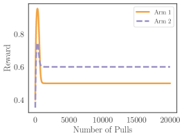
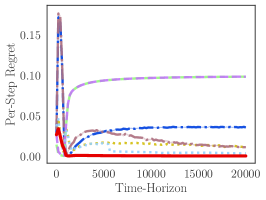
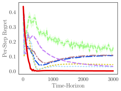
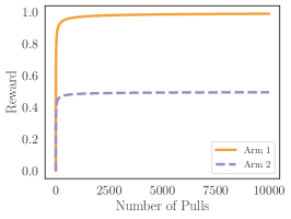
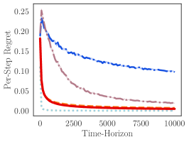
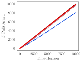
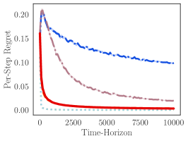
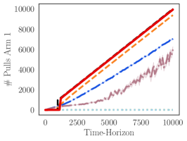
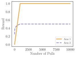
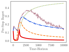
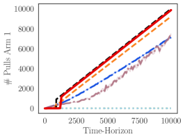
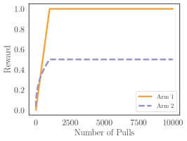
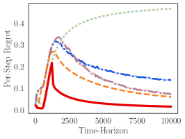
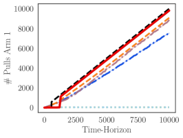
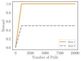
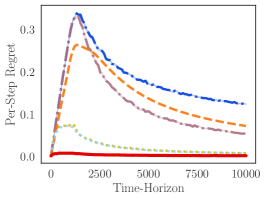
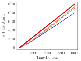
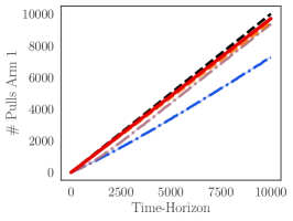
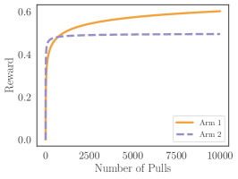
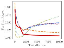
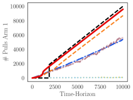
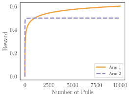
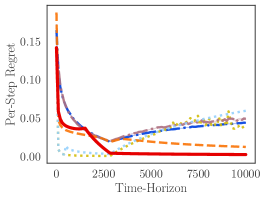
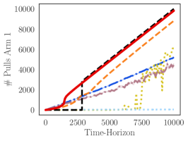
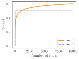
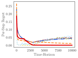
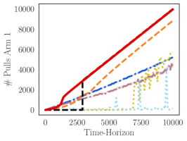
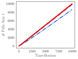
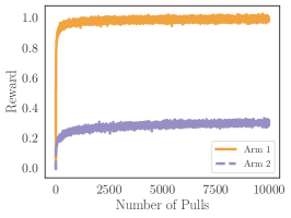
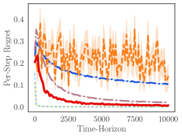
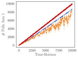
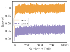
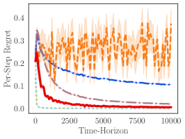
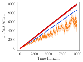
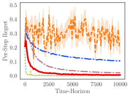
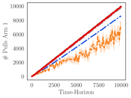
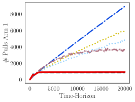
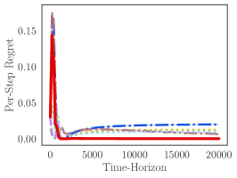
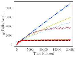
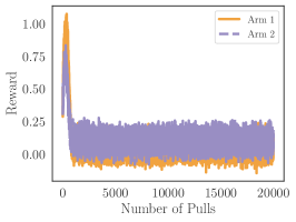
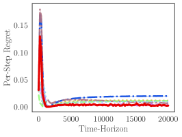
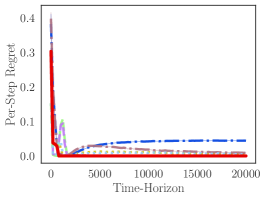
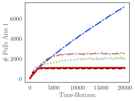
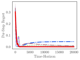
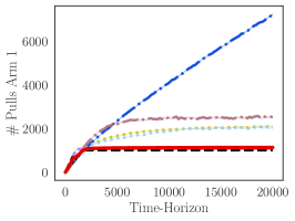
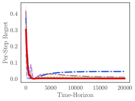
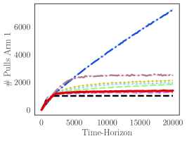
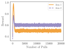
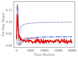
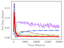
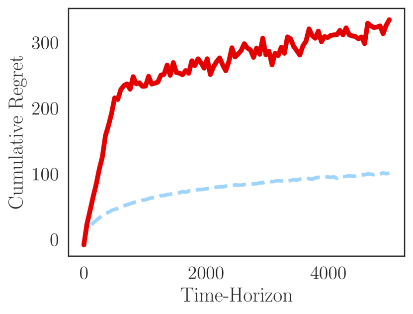
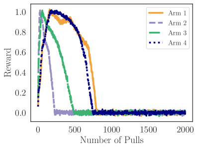
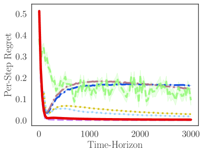
 ), three bandit algorithms designed for nonstationary bandits. All of these algorithms fail on the single-peaked bandit. We propose SPO (
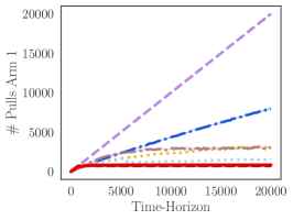
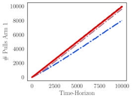
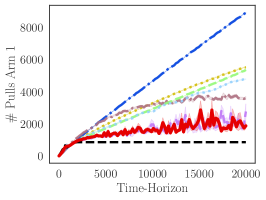
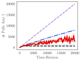
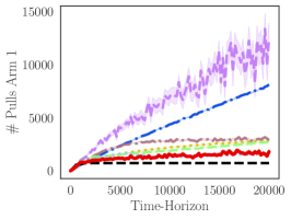
 ) which achieves sub-linear policy regret in single-peaked bandits settings. The right plot shows how often each algorithm pulls the first arm. The plot shows that SPO stops pulling Arm 1 much earlier than the other algorithms, and is much closer to the optimal policy (
 ). For more details on our experiments, see Section 5.
Machine learning (ML) systems increasingly inform or make high-stakes decisions about people, in areas such as credit lending Dobbie et al. (2018), education Marcinkowski et al. (2020), criminal justice Berk and Hyatt (2015), employment Sánchez-Monedero et al. (2020), and beyond. These ML-based decisions can negatively impact already-disadvantaged individuals and communities Sweeney (2013); Buolamwini and Gebru (2018); Angwin et al. (2016). This realization has spawned an active area of research into quantifying and mitigating the disparate effects of ML Dwork et al. (2012); Kleinberg et al. (2017); Hardt et al. (2016). Much of this work has focused on the immediate predictive disparities that arise when supervised learning techniques are applied to batches of training data sampled from a fixed underlying population Dwork et al. (2012); Zafar et al. (2017); Hardt et al. (2016); Kleinberg et al. (2017). While such approaches capture important types of disparity, they fail to account for the long-term effects of present decisions on individuals and communities. Recent work has advocated for shifting the focus to societal-level implications of ML in the long run Liu et al. (2018); Hu et al. (2019); Heidari et al. (2019); Dong et al. (2018); Milli et al. (2019).
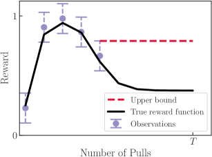
In many real-world domains, decisions made today correspond to the allocation of opportunities and resources that impact the recipients’ future characteristics and capabilities. In such settings, we argue that a socially and ethically acceptable allocation of opportunities must account for the recipients’ long-term potential for turning resources into social utility. As an example, consider the following stylized scenario: Suppose a decision-maker must allocate funds to several communities, all residing in one city, at the beginning of every fiscal period. The communities have distinct racial and wealth compositions, and for historical reasons, they initially have different capabilities to turn their allocated funds into economic prosperity and welfare for members of the community and the city. The decision-maker does not know ahead of time how the economic capabilities of each community will evolve in response to the funds allocated to it. Moreover, he/she can only observe the return on each possible allocation strategy after employing it. While the decision-maker does not know the precise return-on-investment or reward curves associated with each community in advance, domain knowledge may provide him/her with information about the general shape of such curves. For instance, he/she may be able to reliably assume that reward curves are often initially increasing with diminishing marginal returns; and if investment continues beyond a point of saturation, they exhibit decreasing returns to additional investments.
How should a just-minded decision-maker allocate funds in this hypothetical example? Should he/she always aim for equal allocation of funds in every fiscal period to ensure a form of distributive equality today, or are there cases111For example, such considerations may come to the fore once all communities have received a reasonable minimum budget. in which he/she should additionally take each community’s potential for growth into account and allocate funds proportionately? Note that in this example, a myopic decision maker might neglect disadvantaged communities with high long-term potential to turn funds into welfare, and as a result, amplify disparities between advantaged and disadvantaged communities over time. If the decision-maker aims to maximize the city’s long-term economic welfare and prosperity, he/she should prioritize communities that produce higher returns on investment over time. Aside from the utilitarian argument for this objective, it can also be justified through the classic fitness argument to justice and fairness, which states that resources and opportunities must be allocated to those who make the best use of them Sandel (2010); Moulin (2004).222We emphasize that in many domains, considerations such as need and rights should take precedence to fitness as defined in our stylized example. In certain domains, however, fitness can be one of the key criteria in determining whether an allocation is morally acceptable. For the sake of simplicity and concreteness, we solely focus on this particular factor. It is worth noting that our model and findings are equally applicable to settings in which needs or entitlements change in response to the sequence of allocation decisions. This objective motivates the algorithmic question we focus on in this work: how should the decision-maker choose a sequence of allocations to ensure that communities receive funds in proportion to their relative potential for producing high reward for society in the long-run?
Motivated by the above example and numerous other real-world domains in which similar concerns arise,333Additional real-world examples that fit into our model include: allocating policing resources to neighborhoods to maximize safety; allocating funds to research institutions to maximize scientific discoveries and innovations; allocating loans to students to maximize the rate of graduation/ loan pay-back.we study a multi-armed-bandit (MAB) setting in which communities correspond to arms and the reward from each arm evolves every time the decision-maker pulls that arm. We consider a decision-maker who aims to maximize the overall reward obtained within a set time-horizon, but because he/she does not know how the reward curves evolve, he/she is bound to incur some regret. We formulate the decision-maker’s goal in this sequential setting as achieving low policy regret Arora et al. (2012). As Figure 1 shows, conventional no external regret algorithms ignore the impact of their decisions today on the evolution of rewards, so they are prone to spending many of their initial pulls on arms that exhibit high immediate rewards but lack adequate potential for growth.
Technical findings.
We study single-peaked bandits, a new MAB setting with reward functions that are initially increasing and concave in the number of pulls but can become decreasing at some point (Section 2). We introduce Single-Peaked Optimism (SPO), a novel algorithm that considers potential long-term effects of pulling different arms (Section 3). We prove that SPO achieves sub-linear policy regret if rewards can be observed free of noise (Section 3.1). Further, we present an LP-based heuristic that effectively handles noisy reward observations (Section 4). We empirically compare SPO with several standard no-external-regret algorithms and additional baselines, and find that SPO consistently performs better, in particular, for long time horizons (Section 5).
Broader implications.
Our work takes conceptual and technical steps toward modeling and analyzing the long-term implications of ML-informed allocations made over time. From a conceptual point of view, our work showcases the importance of accounting for domain knowledge (here, the general shape of reward curves) and social-scientific insights (e.g., the dynamic by which communities evolve in response to allocation policies) to formulate ML’s long-term impact. Our results draw attention to the necessity of understanding social dynamics of a domain for designing allocation algorithms that improve equity and fairness in the long-run. From a technical perspective, we believe our work can serve as a stepping stone toward designing and analyzing better no-policy regret algorithms for domain-specific reward curves beyond those considered here. Our work is directly applicable to a specific class of reward functions which generalizes and subsumes those in prior work (e.g., (Heidari et al., 2016)). Finally, our novel approach to handling noise allows utilizing the proposed algorithm in more practical settings where observed rewards are expected to be noisy.
1.1 Related Work
Much of the existing work on the social implications of ML focuses on disparities in a model’s predictions Dwork et al. (2012); Zafar et al. (2017); Hardt et al. (2016); Kleinberg et al. (2017). However, these approaches are only suited to evaluate one-shot decision scenarios. In contrast, we formalize disparities that arise when making a sequence of allocation decisions. Recent work has initiated the study of longer-term consequences and effects of ML-based decisions on people, communities, and society. For example, Liu et al. (2018) and Kannan et al. (2019) study how a utility-maximizing decision-maker may interpret and use ML-based predictions. Dong et al. (2018), Hu et al. (2019), and Milli et al. (2019) address strategic classification, a setting in which decision subjects are assumed to respond strategically and untruthfully to the choice of the classification model, and the goal is to design classifiers that are robust to strategic manipulation. Hu and Chen (2018) study the impact of enforcing statistical parity on hiring decisions made in a temporary labor market that precedes a permanent labor market. Mouzannar et al. (2019) and Heidari et al. (2019) model the dynamics of how members of a population react to a selection rule by changing their qualifications (defined in terms of true labels or feature vectors). However, none of the prior articles investigate the community-level implications of ML-based decision-making policies over multiple time-steps.
Another conceptually-relevant line of work studies fairness in online learning Joseph et al. (2016, 2017); Jabbari et al. (2017). Joseph et al. (2016), for example, study fairness in the MAB setting, where arms correspond to socially salient groups (e.g., racial groups), and pulling an arm is equivalent to choosing that group (e.g., to allocate a loan to). They consider an algorithm fair if it never prefers a worse arm to a better one, that is, the arm chosen by the algorithm never has a lower expected reward than the other arms. Similar to Joseph et al. (2016), in our running example, each arm corresponds to a community. However, instead of imposing short-term notions of fairness, we focus on longer-term implications and disparities arising from present decisions.
Our model is based on the MAB framework, which has been established as a powerful tool for modeling sequential decision-making, and has been used successfully for many decades and across a wide range of real-world domains Gittins et al. (2011); Bubeck et al. (2012). From a technical perspective we study a nonstationary bandit problem. In nonstationary bandits (with limits to the change of the reward distributions), modified versions of common bandit algorithms have strong theoretical guarantees and good empirical performance. For example, if the reward distributions only change a small number of times, variants of the upper confidence bound algorithm (UCB) such as discounted or sliding-window UCB perform well Garivier and Moulines (2011). Similarly, if there is a fixed budget on how much the rewards can change, R-EXP3, a variant of the popular EXP3 algorithm for adversarial bandits Auer et al. (2002), guarantees low regret Besbes et al. (2019). In this work, we do not restrict how much the rewards can change, but instead restrict the functional shape of the reward functions to be first increasing and concave before switching to decreasing. This is somewhat similar to rotting bandits Levine et al. (2017) and recharging bandits Kleinberg and Immorlica (2018), but distinct from them in crucial ways. In contrast to rotting bandits, where the rewards decrease when pulling an arm more often, our reward functions first increase and only later decrease with the number of pulls. In contrast to recharging bandits, where rewards are increasing and concave in the amount of time an arm has not been pulled, we consider a bandit setting with rewards depending on the number of times an arm has been pulled. We consider reward functions that exhibit a “unimodal” shape. However, our setting is very different from unimodal bandits, which are stationary bandit models with a unimodal structure across arms Yu and Mannor (2011); Combes and Proutiere (2014).
The setting by Heidari et al. (2016) is closest to ours. They consider two separate models, one with rewards that are increasing and concave, and another with decreasing rewards in the number of pulls of an arm. While (Heidari et al., 2016) provides different algorithms for these two cases, we present a single algorithm that can adapt to both settings and beyond, while matching the respective asymptotic policy regret bounds in (Heidari et al., 2016) (cf. Appendix B). Additionally, in contrast to (Heidari et al., 2016) which primarility studies noise-free observations, we provide an effective heuristic for handling noise.
For an extended discussion of prior work, see Appendix A.
2 The Single-Peaked Bandit Setting
We consider a multi-armed bandit (MAB) with arms , corresponding, e.g., to the different communities in our introductory example. At each time step , the decision-maker pulls one arm and observes its immediate reward, e.g., the short-term outcome of an investment in a community. The decision-maker aims to achieve the highest cumulative reward within the fixed time horizon , e.g., he/she wants to get the best total return-on-investment over years. Each arm has an underlying reward function . When the decision-maker pulls arm for the -th time (), he/she observes reward . Later, in Section 4, we study noisy reward observations of the form , but for now, let’s assume observed rewards are noise-free. We denote the cumulative reward of arm after pulls by .
A deterministic policy is a sequence of mappings from observed action-reward histories to arms, where maps histories of length to the next arm to be pulled:
The cumulative reward of a policy only depends on how often it pulls each arm, so it is determined by a tuple where denotes how often pulls arm within the time horizon . Note that . We can write the cumulative reward of a policy as:
Let denote the space of all possible deterministic policies, and be an optimal policy, that is, a policy achieving the highest possible cumulative reward. The decision-maker does not know the reward functions (’s) in advance, so he/she cannot find an optimal policy ahead of time. Instead, he/she can aim to design a (possibly stochastic) policy that minimizes the policy regret: . Given a fixed set of reward functions, we say an algorithm that follows policy over time horizon has sub-linear policy regret, if
It is in general impossible to achieve sub-linear policy regret in an adversarial bandit setting Arora et al. (2012), and we have to make additional assumptions about the shape of the reward functions . In this work, we assume that the underlying reward functions are initially increasing and concave, then decreasing.
Definition 1 (Single-peaked bandit).
We call a single-peaked reward function, if there exists a tipping points such that increases monotonically in and is concave up to , and then decreases monotonically for . We call a bandit with single-peaked reward functions a single-peaked bandit.
Note that bandits with monotonically increasing or decreasing reward functions are single-peaked bandits with and , respectively.
3 SPO: A New No-Policy-Regret Algorithm
Our algorithm operationalizes the principle of optimism in the face of uncertainty, which has been successfully applied with different interpretations to a wide range of MAB problems Bubeck et al. (2012). Our interpretation of the principle is as follows: At each time step, pull the arm with the highest optimistic future reward. The reward functions of a single-peaked bandit are first increasing and concave, then become decreasing. Therefore, we can define the future optimistic reward in the increasing phase using concavity and in the decreasing phase using monotonicity of the reward function. In the increasing concave phase, we estimate the optimistic future reward as
where . Defined this way, is a linear optimistic approximation of future rewards from arm after it has been pulled times within the first pulls. Similarly, for the decreasing phase, we can define
In the increasing phase, we use the fact that the reward will increase at most linearly, and in the decreasing phase we use that it will at best remain constant.
The Single-Peaked Optimism algorithm (SPO, Algorithm 1) performs two main steps at every round :
-
1.
Pull the arm that maximizes where is the number of times the algorithm has pulled arm so far.
-
2.
Update the optimistic future rewards .
For technical reasons, we add an initial phase in which we pull each arm times, which only adds sub-linear policy regret, but simplifies the analysis (see Appendix C).
Our analysis formalizes the observation that while SPO may initially overestimate the future reward of an arm that grows at a high rate, it will stop pulling that arm as soon as it ceases to live up to the optimistic expectations.
3.1 Regret Analysis
Next, we present our main theoretical result, which establishes the sub-linear policy regret of SPO. All omitted proofs and technical material can be found in Appendix C.
Theorem 1.
[informal statement] For any (noise-free) single-peaked bandit, SPO achieves sub-linear policy regret.
The proof consists of several steps: we first observe that all single-peaked reward functions have finite asymptotes (Lemma 3, Appendix C), which follows from the monotone convergence theorem. Then, we show that for sufficiently large time horizons, always pulling the single arm with the highest asymptote would lead to sub-linear policy regret (Lemma 4, Appendix C). Finally, the key step of the proof is to show that SPO pulls all arms with suboptimal asymptotes less than linear in . Together these steps imply the sub-linear policy regret of SPO.
4 An LP-based Heuristics to Handle Noise
So far we have assumed the decision-maker can observe rewards free of noise. In this section, we describe how to find an upper bound on the future reward from noisy observations. This allows us to extend SPO to noisy observation.
Assume that when pulling arm for the -th time, we observe where is a random noise term. We start by assuming that the magnitude of the noise is bounded , and is known for each arm. We can then define and to obtain confidence intervals for the true reward such that with probability .
We first extend our algorithm to this case of bounded noise, and then relax this assumption to confidence intervals that contain the true value with probability less than .
Decreasing phase.
For arms in their decreasing phase, we define the optimistic future return as using the confidence interval .
Increasing phase.
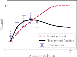
For arms in their increasing phase, we combine our noise confidence intervals with our knowledge that the function is concave. Concretely, we find the monotone concave function with the highest cumulative future reward that can explain past observations. We can phrase this as solving the following linear program (LP) for each arm :
| () |
where is the number of times arm has been pulled up to time . The optimization variables correspond to the values of the reward function after pulls of arm . The constraints encode that the true reward function is bounded, consistent with past observations, increasing, and concave, in that order. Hence, a feasible solution to the LP corresponds to a possible reward function and an optimal solution provides a tight upper bound on future rewards.
Theorem 2.
Let be a concave, increasing function with confidence bounds such that for . Let be the solution to (). Then, . Furthermore, there exists a concave, increasing function, , such that .
We can extend SPO to noisy observations, by solving the LP () every time we update the future optimistic reward for a given arm. If the LP does not have a feasible solution, we can infer that the arm is in its decreasing phase, and use a corresponding upper bound. Figure 2 illustrates both cases.
Unbounded noise.
We can readily extend this approach to unbounded noise with confidence intervals.
Corollary 1.
Let be a concave, increasing function. Suppose that for any and observation we can find a confidence interval such that with probability at least . Let be the solution to (). Then for any , we can choose such that with probability at least .
The proof sketch goes as follows: The probability that within the remainder of time horizon , at least one true reward value falls outside of its confidence interval is upper bounded by . For the given , we can choose so that the probability of any true reward being outside its confidence interval is bounded by . More precisely, we can write:
With the above choice for , the optimistic future reward is estimated correctly with probability at least .
5 Experiments
In this section, we empirically investigate the effectiveness of our noise-handling approach on several datasets.444Code to reproduce all of our experiments can be found at https://github.com/david-lindner/single-peaked-bandits.
Setup.
We consider three datasets: (1) a set of synthetic reward functions, (2) a simulation of a user interacting with a recommender system, and (3) a dataset constructed from the FICO credit scoring data. We compare SPO with six baselines: (1) a greedy algorithm that always pulls the arm that provided the highest reward at the last pull, (2) a one-step-optimistic variant of SPO that pulls the arm with the highest upper bound on the reward at the next pull, (3) EXP3, a standard no-external-regret algorithm for adversarial bandits Auer et al. (2002), (4) R-EXP3, a modification of EXP3 for non-stationary bandits Besbes et al. (2019), (5) discounted UCB (D-UCB), and (6) sliding window UCB (SW-UCB), two adaptations of UCB to nonstationary bandits Garivier and Moulines (2011).
Illustrations on synthetic data.
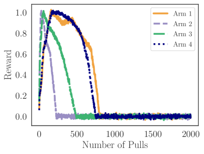
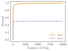
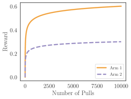
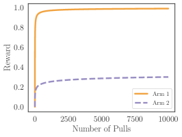
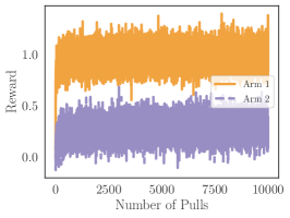
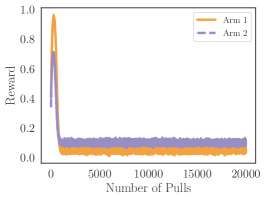
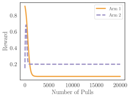
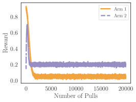
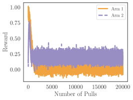
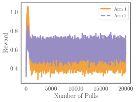
We first perform a series of experiments on single-peaked bandits with two arms, and synthetic reward functions with Gaussian noise. To this end we define a class of single-peaked functions and combine them into multiple single-peaked bandits with two arms each. In Figure 1 we highlight one experiment in which algorithms that minimize external regret fail. The figure shows how SPO avoids this kind of failure by minimizing policy regret. In Appendix D we provide more detailed results comparing SPO to the baselines on various synthetic reward functions, including the monotonic functions proposed by Heidari et al. (2016), and evaluate the effect of varying the observation noise. We find that SPO matches the performance of the baselines in all cases and significantly outperforms them in some. Further, we show that SPO can also handle stationary MABs, where arms have fixed reward distributions.
FICO credit lending data.
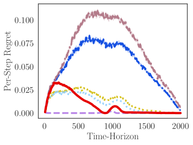
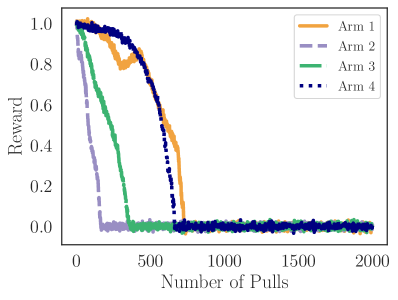
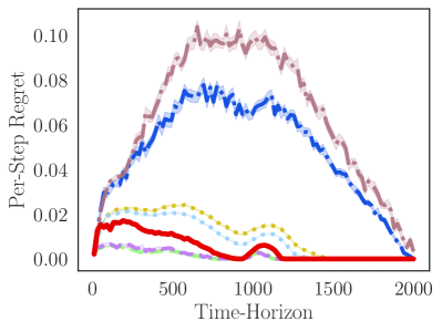
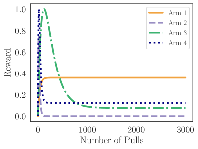
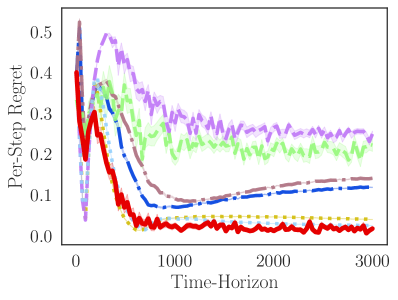
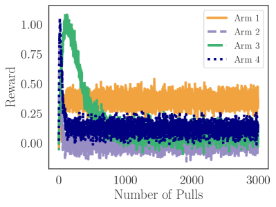
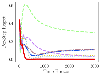
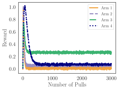
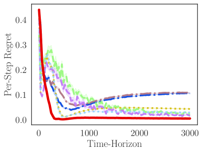
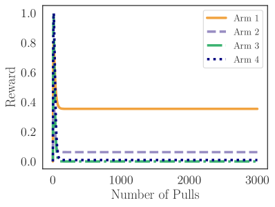
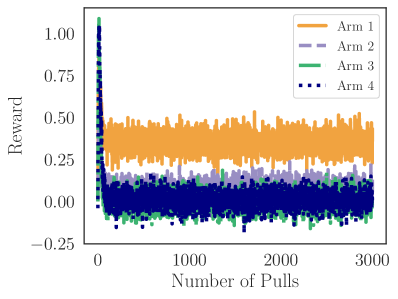
Motivated by our initial example of a budget planner in Section 1, we simulate a credit lending scenario based on the FICO credit scoring dataset from 2003 Reserve (2007). We pre-process the data using code provided by previous work Hardt et al. (2016); Liu et al. (2018). The dataset contains four ethnic groups: ’Asian’, ’Black’, ’Hispanic’ and ’White’. Each group has a distribution of credit-scores and an estimated mapping from credit-scores to the probability of repaying a loan. We use this group-level data to simulate a population of individuals applying for a loan. Each individual belongs to one ethnic group and has a credit score sampled from the group’s distribution and a probability of repaying a loan.
We consider a hypothetical decision-making scenario in which at each round, there is exactly one loan applicants from each group. In each time step, the decision-maker (i.e., a bank) can approve only one loan applicant. We are interested in the long-term impact of decision-maker’s choices on the underlying groups. As discussed in Section 1, we argue that a fair decision-maker will allocate loans according to the groups’ long-term potential to turn them into welfare/prosperity, which is measured by the per-group reward functions in this simulation. In other words, policy regret is our measure of long-term disparity and achieving low policy regret improves the fairness of resource allocation decisions.
To simulate this situation based on the FICO dataset, we first sample applicants from each group. We assume the decision-maker always approves the loan of the applicant with the highest credit score within a given group; hence, we order the applicants decreasing by their credit score. Thereby, we reduce the problem to the decision-maker deciding between four arms to pull, each corresponding to one group. We interpret pulling an arm as approving the load on the highest scoring applicant within the corresponding group. However, the credit scores do not directly correspond to the reward of pulling an arm. Rather we want to define a reward function that quantifies the benefit/loss of giving out a loan to a group.555We also investigated a variant of this setting considering only the utility of a loan to the decision-maker, see Appendix D. We follow Liu et al. (2018), and measure the impact on a group as the change in mean credit score for this group. Liu et al.’s model assumes an increase in credit score of points for a repaid loan and a decrease of points for a defaulted loan, while the credit score is always being clipped to the range . Finally, we rescale the rewards to .
The resulting reward functions increase at first because the first individuals in each group are highly credit-worthy and them paying back their loan increases the mean credit score for the group. The reward functions are concave because as the decision-maker gives more loans to a group he/she starts to give loans to less creditworthy individuals. Eventually, the reward functions start to decrease because giving loans to individuals who cannot pay them back decreases the average credit score of the group. Hence, this setup can be approximately modelled as a single-peaked bandit.
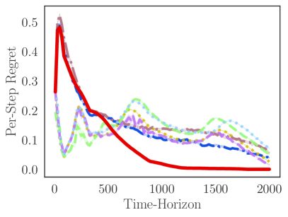
Figure 3(a) shows results of running SPO in this setup. Overall, SPO strictly outperforms the baselines over long time horizons. For short time horizons we find that simple greedy approaches or UCB variants can perform favorably.
Synthetic recommender system data.
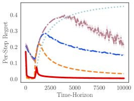
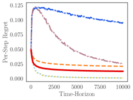
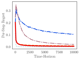
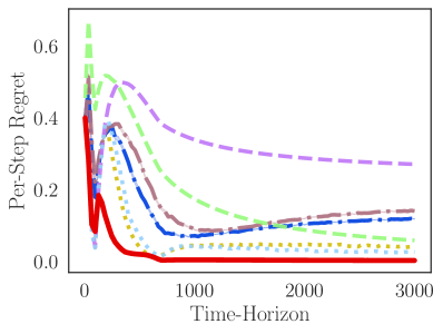
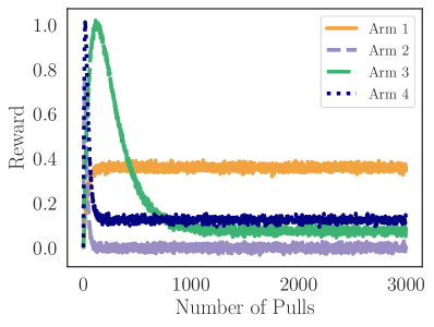
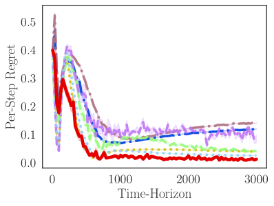
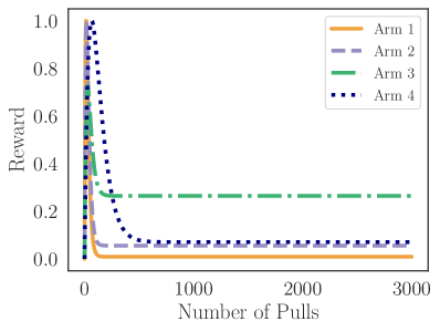
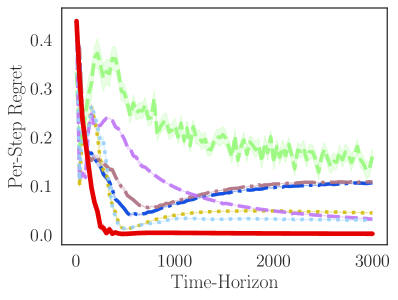
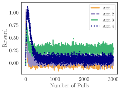
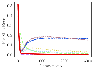
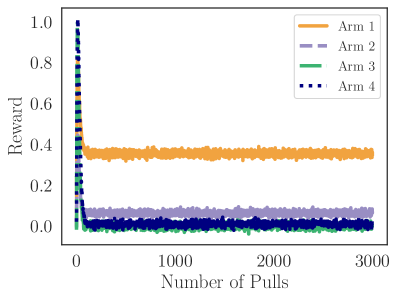
Recent work shows that strategies minimizing external regret can perform poorly in the context of recommender systems, due to negative feedback loops Jiang et al. (2019); Warlop et al. (2018); Mladenov et al. (2020); Chaney et al. (2018). Here, we focus on one concrete problem that can arise: many recommender systems exhibit a bias towards recommending particularly engaging or novel content that leads to high instantaneous reward, disregarding the long-term benefit and cost to the user. We argue that this situation is analogous to our example of a budget maker, and that a recommender system should aim to maximize it’s users’ long-term benefit.
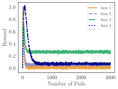
Motivated by this observation, we simulate a system that recommends content, e.g., articles or videos, to a user and receives feedback about how much the user engaged with the content. For simplicity, we assume the user’s engagement with a piece of content is driven by two factors only: (i) the user’s inherent preferences, and (ii) a novelty factor which makes new content more engaging to the user. We assume that the user’s inherent preferences stay constant, but the novelty factor decays when showing an item more often. Note that an algorithm that minimizes external regret would show content with high novelty and neglect content that is a better match for the user’s inherent preferences. An algorithm that minimizes policy regret would select the content that best matches the user’s inherent preferences in the long-run.
We simulate the user’s feedback with a reward function for each item that can be recommended. Each item has an inherent value to the user, a novelty factor , and decay factors and . The reward is for never showing an item, and subsequent rewards are defined as
The second term in the expression models the novelty of an item which decays when showing it more often. The third term models the tendency of the reward to move towards how much the user values the item inherently. The resulting rewards increase at first due to the novelty of an item and decrease later as the novelty factor decays. For simplicity we model all effects that are not captured by this stylized model as Gaussian noise on the observed rewards.
Figure 3(b) shows that SPO significantly outperforms the baselines for long time horizons, at the cost of worse performance for short time horizons. This results indicates that if a decision-maker acts on a short time-horizon classical bandit algorithms perform well. However, if the decision-maker aims to achieve a good long-term impact, SPO is preferable. We present results on additional instances of the recommender system simulation in Appendix D.
6 Conclusion
Motivated by several real-world domains, we studied single-peaked bandits in which the reward from each arm is initially increasing then decreasing in the number of pulls of the arm. We introduced Single-Peaked Optimism (SPO), an algorithm that achieves sub-linear policy regret in single-peaked bandits. Our findings highlight the importance of understanding the long-term implications of ML-based decisions for impacted communities and society at large, and utilizing domain knowledge, e.g., regarding social- and population-level dynamics stemming from decisions today, to design appropriate sequences of allocations that do not amplify historical disparities.
Limitations.
We argued that single-peaked bandits are a useful model to provide insights about allocation decisions in a range of practical domains, e.g., allocating loans to communities, allocating funds to research institutions, or allocating policing resources to districts. However, single-peaked bandits can also be too restrictive in domains where the evolution of rewards are more nuanced, e.g., if rewards can later increase again after first decreasing. We emphasize that single-peaked reward functions are one among many reasonable classes of reward functions that are interesting to study from an algorithmic perspective. We consider our work as an starting point to look into more complex dynamics in future work.
Future work.
We hope that our work draws the research community’s attention to the study of policy regret for typical reward-evolution curves. Additional directions for future work include (1) establishing regret bounds for settings with arbitrary noise distributions, (2) providing instance-specific (and potentially tighter) regret bounds for Single-Peaked Optimism, and finally (3) more broadly characterizing the limits of “optimism in the face of uncertainty” principle in achieving low policy regret.
Acknowledgements
Lindner was partially supported by Microsoft Swiss JRC. This work was in part done while Heidari was a postdoctoral fellow at ETH Zurich. Heidari acknowledges partial support from NSF IIS2040929. Any opinions, findings, and conclusions, or recommendations expressed in this material are those of the authors and do not necessarily reflect the views of the National Science Foundation, or other funding agencies.
References
- Angwin et al. [2016] Julia Angwin, Jeff Larson, Surya Mattu, and Lauren Kirchner. Machine bias. Propublica, 2016.
- Arora et al. [2012] Raman Arora, Ofer Dekel, and Ambuj Tewari. Online bandit learning against an adaptive adversary: from regret to policy regret. In ICML, 2012.
- Auer et al. [2002] Peter Auer, Nicolo Cesa-Bianchi, Yoav Freund, and Robert E Schapire. The nonstochastic multiarmed bandit problem. SIAM journal on computing, 32(1):48–77, 2002.
- Berk and Hyatt [2015] Richard Berk and Jordan Hyatt. Machine learning forecasts of risk to inform sentencing decisions. Federal Sentencing Reporter, 27(4):222–228, 2015.
- Besbes et al. [2019] Omar Besbes, Yonatan Gur, and Assaf Zeevi. Optimal exploration–exploitation in a multi-armed bandit problem with non-stationary rewards. Stochastic Systems, 9(4):319–337, 2019.
- Bubeck et al. [2012] Sébastien Bubeck, Nicolo Cesa-Bianchi, et al. Regret analysis of stochastic and nonstochastic multi-armed bandit problems. Foundations and Trends® in Machine Learning, 5(1):1–122, 2012.
- Buolamwini and Gebru [2018] Joy Buolamwini and Timnit Gebru. Gender shades: Intersectional accuracy disparities in commercial gender classification. In Conference on Fairness, Accountability, and Transparency, 2018.
- Chaney et al. [2018] Allison JB Chaney, Brandon M Stewart, and Barbara E Engelhardt. How algorithmic confounding in recommendation systems increases homogeneity and decreases utility. In Conference on Recommender Systems, 2018.
- Combes and Proutiere [2014] Richard Combes and Alexandre Proutiere. Unimodal bandits: Regret lower bounds and optimal algorithms. In ICML, 2014.
- Dobbie et al. [2018] Will Dobbie, Andres Liberman, Daniel Paravisini, and Vikram Pathania. Measuring bias in consumer lending. Technical report, National Bureau of Economic Research, 2018.
- Dong et al. [2018] Jinshuo Dong, Aaron Roth, Zachary Schutzman, Bo Waggoner, and Zhiwei Steven Wu. Strategic classification from revealed preferences. In Conference on Economics and Computation, 2018.
- Dwork et al. [2012] Cynthia Dwork, Moritz Hardt, Toniann Pitassi, Omer Reingold, and Richard Zemel. Fairness through awareness. In ITCS, 2012.
- Ensign et al. [2017] Danielle Ensign, Sorelle A. Friedler, Scott Neville, Carlos Eduardo Scheidegger, and Suresh Venkatasubramanian. Decision making with limited feedback: Error bounds for predictive policing and recidivism prediction. In Conference on Fairness, Accountability, and Transparency, 2017.
- Ensign et al. [2018] Danielle Ensign, Sorelle A. Friedler, Scott Neville, Carlos Eduardo Scheidegger, and Suresh Venkatasubramanian. Runaway feedback loops in predictive policing. In Conference on Fairness, Accountability, and Transparency, 2018.
- Garivier and Moulines [2011] Aurélien Garivier and Eric Moulines. On upper-confidence bound policies for switching bandit problems. In International Conference on Algorithmic Learning Theory, 2011.
- Gittins et al. [2011] John Gittins, Kevin Glazebrook, and Richard Weber. Multi-armed bandit allocation indices. John Wiley & Sons, 2011.
- Hardt et al. [2016] Moritz Hardt, Eric Price, and Nati Srebro. Equality of opportunity in supervised learning. In Advances in Neural Information Processing Systems, 2016.
- Heidari et al. [2016] Hoda Heidari, Michael J. Kearns, and Aaron Roth. Tight policy regret bounds for improving and decaying bandits. In IJCAI, 2016.
- Heidari et al. [2019] Hoda Heidari, Vedant Nanda, and Krishna P Gummadi. On the long-term impact of algorithmic decision policies: Effort unfairness and feature segregation through social learning. In ICML, 2019.
- Hu and Chen [2018] Lily Hu and Yiling Chen. A short-term intervention for long-term fairness in the labor market. In WWW, 2018.
- Hu et al. [2019] Lily Hu, Nicole Immorlica, and Jennifer Wortman Vaughan. The disparate effects of strategic manipulation. In Conference on Fairness, Accountability, and Transparency, 2019.
- Jabbari et al. [2017] Shahin Jabbari, Matthew Joseph, Michael Kearns, Jamie Morgenstern, and Aaron Roth. Fairness in reinforcement learning. In ICML, 2017.
- Jiang et al. [2019] Ray Jiang, Silvia Chiappa, Tor Lattimore, András György, and Pushmeet Kohli. Degenerate feedback loops in recommender systems. In Conference on AI, Ethics, and Society, 2019.
- Joseph et al. [2016] Matthew Joseph, Michael Kearns, Jamie Morgenstern, and Aaron Roth. Fairness in learning: Classic and contextual bandits. In Advances in Neural Information Processing Systems, 2016.
- Joseph et al. [2017] Matthew Joseph, Michael Kearns, Jamie Morgenstern, Seth Neel, and Aaron Roth. Fair algorithms for infinite contextual bandits. In Conference on Fairness, Accountability, and Transparency, 2017.
- Kannan et al. [2019] Sampath Kannan, Aaron Roth, and Juba Ziani. Downstream effects of affirmative action. In Conference on Fairness, Accountability, and Transparency, 2019.
- Kleinberg and Immorlica [2018] Robert Kleinberg and Nicole Immorlica. Recharging bandits. In Annual Symposium on Foundations of Computer Science (FOCS), pages 309–319, 2018.
- Kleinberg et al. [2017] Jon Kleinberg, Sendhil Mullainathan, and Manish Raghavan. Inherent trade-offs in the fair determination of risk scores. In ITCS, 2017.
- Levine et al. [2017] Nir Levine, Koby Crammer, and Shie Mannor. Rotting bandits. In Advances in Neural Information Processing Systems, 2017.
- Liu et al. [2018] Lydia T Liu, Sarah Dean, Esther Rolf, Max Simchowitz, and Moritz Hardt. Delayed impact of fair machine learning. In ICML, 2018.
- Marcinkowski et al. [2020] Frank Marcinkowski, Kimon Kieslich, Christopher Starke, and Marco Lünich. Implications of AI (un-) fairness in higher education admissions: the effects of perceived AI (un-) fairness on exit, voice and organizational reputation. In Conference on Fairness, Accountability, and Transparency, 2020.
- Milli et al. [2019] Smitha Milli, John Miller, Anca D Dragan, and Moritz Hardt. The social cost of strategic classification. In Conference on Fairness, Accountability, and Transparency, 2019.
- Mladenov et al. [2020] Martin Mladenov, Elliot Creager, Omer Ben-Porat, Kevin Swersky, Richard Zemel, and Craig Boutilier. Optimizing long-term social welfare in recommender systems: A constrained matching approach. In ICML, 2020.
- Moulin [2004] Hervé Moulin. Fair division and collective welfare. MIT press, 2004.
- Mouzannar et al. [2019] Hussein Mouzannar, Mesrob I Ohannessian, and Nathan Srebro. From fair decision making to social equality. In Conference on Fairness, Accountability, and Transparency, 2019.
- Reserve [2007] US Federal Reserve. Report to the congress on credit scoring and its effects on the availability and affordability of credit. Board of Governors of the Federal Reserve System, 2007.
- Robbins [1952] Herbert Robbins. Some aspects of the sequential design of experiments. Bulletin of the American Mathematical Society, 58(5):527–535, 1952.
- Sánchez-Monedero et al. [2020] Javier Sánchez-Monedero, Lina Dencik, and Lilian Edwards. What does it mean to ’solve’ the problem of discrimination in hiring? social, technical and legal perspectives from the uk on automated hiring systems. In Conference on Fairness, Accountability, and Transparency, 2020.
- Sandel [2010] Michael J Sandel. Justice: What’s the right thing to do? Macmillan, 2010.
- Sweeney [2013] Latanya Sweeney. Discrimination in online ad delivery. Queue, 11(3):10, 2013.
- Tekin and Liu [2012] Cem Tekin and Mingyan Liu. Online learning of rested and restless bandits. Transactions on Information Theory, 58(8):5588–5611, 2012.
- Warlop et al. [2018] Romain Warlop, Alessandro Lazaric, and Jérémie Mary. Fighting boredom in recommender systems with linear reinforcement learning. In Advances in Neural Information Processing Systems, 2018.
- Whittle [1988] Peter Whittle. Restless bandits: Activity allocation in a changing world. Journal of applied probability, pages 287–298, 1988.
- Yu and Mannor [2011] Jia Yuan Yu and Shie Mannor. Unimodal bandits. In ICML, 2011.
- Zafar et al. [2017] Muhammad Bilal Zafar, Isabel Valera, Manuel Gomez Rodriguez, and Krishna P. Gummadi. Fairness beyond disparate treatment & disparate impact: Learning classification without disparate mistreatment. In WWW, 2017.
Appendix A More Details on Related Work
In this section we give more details on related work.
External vs. policy regret.
The vast majority of existing algorithms for the well-studied MAB setting aim to minimize the so-called external regret. External regret is the difference between the total reward collected by an online algorithm and the maximum reward that could have been collected by pulling the best/optimal arm on the same sequence of rewards as the one generated by the online algorithm. Existing work on MAB often focuses on one of the following two settings: first, the statistical setting in which the reward from each arm is assumed to be sampled from a fixed, but unknown distribution Robbins (1952); Gittins et al. (2011); Auer et al. (2002), and second, the adversarial setting where an adversary—who is capable of reacting to the choices of the decision-maker—determines the sequence of rewards Auer et al. (2002). As discussed by Arora et al. (2012), the notion of external regret fails to capture the actual regret of an online algorithm compared to the optimal sequence of actions it could have taken when the adversary is adaptive. Policy regret is defined to address this counterfactual setting. Arora et al. show that if the adaptive adversary has bounded memory, then a variant of traditional online learning algorithms can still guarantee no-policy-regret. If the adversary does not have bounded memory, as is the case in our setting, no algorithm can achieve no-policy-regret in general. Hence, additional assumptions are required, such as the ones we make when defining single-peaked bandits.
Restless and rested bandits.
Nonstationary bandits are called restless if the rewards of an arm can change in each timestep, or rested if the reward of an arm can only change when the arm is pulled Tekin and Liu (2012). Restless bandits model changes in the environment due to external effects Whittle (1988), whereas rested bandits model changes to the environment caused by interactions of the decision maker with the environment. Such feedback effects are the focus of our work, and hence we consider a rested nonstationary bandit.
Feedback loops as a source of unfairness.
At a high-level, feedback loops occur when outputs of a system influence its inputs in future rounds, and this cause-and-effect circuit amplifies or inhibits the system Ensign et al. (2017, 2018); Liu et al. (2018).
Ensign et al. (2017), for example, study feedback loops in the context of recidivism prediction, that is, predicting if an inmate will re-offend within a fixed time after being released, and predictive policing, that is, allocating police patrols to city districts based on historical crime data. In both cases, the decision-maker faces a partial monitoring problem: the decision-maker only receives feedback if he/she takes specific actions (e.g., release an inmate or send a patrol). Ensign et al. (2018) show that commonly-used algorithms for predictive policing suffer from a specific type of feedback loop: if police patrols are assigned based on historical crime data, the assignment rate of police officers to neighborhoods can quickly become highly disproportionate to the actual crime rates of the neighborhoods.
Feedback loops can also occur in recommender systems Jiang et al. (2019); Warlop et al. (2018); Mladenov et al. (2020); Chaney et al. (2018), which motivated some of the simulation experiment in Section 5. Jiang et al. (2019) argue that feedback loops can give rise to ”echo chamber” and ”filter bubble effects”, and Chaney et al. (2018) argue that they lead to more homegenity and lower utility for the users. Warlop et al. (2018) suggest that minimizing external regret is sub-optimal for recommender systems because the user’s preferences can change depending on what is recommended to them, and Mladenov et al. (2020) propose to maximize the long-term social welfare instead of short-term reward. These interpretations of feedback loops in recommender systems are in line with the main conceptual argument of our work: when deploying ML-based systems to make decisions that affect humans, one should focus on maximize their long-term well-being instead of sacrificing it for short-term reward.
We argue that these different kinds of feedback loops are a consequence of deploying algorithms that minimize external regret instead of policy regret, and, therefore, do not take into account the long-term effects of their decisions.
Appendix B Monotone Bandits
In this section, we describe bandits with monotonically increasing or decreasing reward functions, as described by Heidari et al. (2016). We show that these are special cases of single-peaked bandits, and that SPO achieves the same asymptotic policy regret as the algorithms introduced by Heidari et al..
B.1 Increasing Reward Functions
Heidari et al. consider reward functions that are monotonically increasing and concave which correspond to single-peaked bandits with for every arm. With this observation we receive sub-linear policy regret of SPO in this setting as a corollary of Theorem 1.
Lemma 1.
For any set of bounded, concave and increasing reward functions , the policy regret of SPO is sub-linear.
This results shows that our algorithm matches the asymptotic performance of Algorithm 1 by Heidari et al. in the case of increasing reward functions.
B.2 Decreasing Reward Functions
Further, Heidari et al. study bandits with monotonically decreasing reward functions, which are single-peaked bandits with . Heidari et al. show that for decreasing reward functions the optimal policy in hindsight always pulls the arm with the highest instantaneous reward. This immediately gives a constant-policy-regret algorithm that greedily pulls the arms that gave the highest reward at the last pull.
It is straightforward to show that in the case of monotonically decreasing reward functions, SPO is equivalent to the greedy algorithm after the initial phase of pulling all arms. In particular, this implies that it achieves sub-linear policy regret for this case as well.
Lemma 2.
For any set of monotonically decreasing reward functions and a time horizon , SPO greedily pulls the arms that gave the highest reward at the last pull after its initial phase. Therefore, it achieves sub-linear policy regret.
Proof.
After pulling every arm times, SPO will always update the optimistic future reward to be
after has been pulled times because the reward functions are decreasing. At each time step, SPO then pulls an arm . For fixed and
Hence, at each time step SPO pulls an arm that gave the highest reward at the last pull. Heidari et al. show that this behavior is optimal. Therefore SPO only incurs policy regret of order during its initial phase. In particular, the policy regret is sub-linear. ∎
While SPO achieves sub-linear regret, it does not match the performance of a greedy algorithm which achieves constant policy regret Heidari et al.. In situations where the reward functions are known to be decreasing a greedy approach is therefore preferrable. If, however, reward functions might be increasing or decreasing SPO can still achieve sub-linear regret.
Appendix C Proofs of Theoretical Statements
This section contains detailed proofs for all results presented in the main paper.
C.1 Noise-free Observations
Definition 2.
We call arms with a single-peaked reward function with asymptotically increasing, and all other single-peaked arms asymptotically decreasing.
Lemma 3.
All arms of a single-peaked bandit have an asymptote, i.e., a finite limit , which is bounded between and , i.e., .
Proof.
This follows from the monotone convergence theorem:
Theorem (Monotone Convergence).
If is a monotone sequence of real numbers ( or for all ) then this sequence has a finite limit if and only if it is bounded.
In our case, all are bounded between and . Asymptotically increasing arms are monotone and asymptotically decreasing arms are monotone for all . Hence the theorem applies to both cases and gives a finite limit between and for each arm. ∎
Lemma 4.
Let . For any let be the policy that pulls the -th arm times and does not pull any other arm. Then, achieves sub-linear policy regret.
Proof.
Let denote the number of times pulls arm for time horizon . Then
Observe that
And because also
Hence for any there exists a such that for any and all
Then with
Let and consider a general . Then because is increasing
We can use this to upper bound the reward of the optimal policy
where in the last step we use . Dividing by and taking the limit gives us
Because this has to hold for all , it implies
| (1) |
Not consider the policy . It only pulls arm and therefore achieves reward
Because we have
and this means
In particular for any there exists a such that for
where we defined . Therefore we get
and
Because this has to hold for all we end up with
| (2) |
Combining eqs. (1) and (2) gives
which gives the desired result
because
∎
See 1
Theorem (formal statement of Theorem 1).
Let be the arms of a single-peaked bandit. Denote the SPO algorithm by . Then SPO achieves sub-linear policy regret, i.e.,
Proof.
Let , let arm be in and be the policy that only pulls arm . We will show that
which implies the theorem because of lemma 4 and
We now go on to show two things: (i) pulling arms adds sub-linearly to the reward difference between and and (ii) the number of times pulls arms is sub-linear in .
To show (i) we modify a Lemma by Heidari et al. (2016) to hold for single-peaked reward functions instead of monotonically increasing reward functions.
Lemma 5 (Adaptation of Lemma 2 in Heidari et al. (2016)).
Let and let denote the number of times pulls arm . Then
holds for single-peaked bandits.
Proof of Lemma.
If is pulled times, it can not cause the algorithm to suffer linear policy regret. Now consider a subset of consisting of any suboptimal arm which is pulled times by the algorithm.
Given that all arms not in are pulled less than times, we have that .
Let be the arm for which is the smallest, i.e. the arm with optimal asymptote that has the lowest average reward. We have
where in the last step we used that is constant and . In total we now have
It only remains to show that
We have and therefore
|
|
which means . Together this gives the desired result. ∎
Lemma 5 shows that whenever pulls an arm in it incurs sub-linear regret, which concludes step (i).
It remains to show (ii), that is the number of times pulls arms is sub-linear in . For this we use the initial phase in which the algorithm pulls each arm times. Importantly, this phase only adds sub-linear regret, and after this phase we can assume to be large enough such that for every arm
| (3) |
where
is the number of times the algorithm pulls arm and
Let . We will show that by using . We show that which implies .
Assume this was not the case, then we could find an infinite subsequence of ’s, which we label such that for every
Dropping the indices, we just write to mean for an arbitrary .
Let be the last timestep at which the algorithm pulls arm within time horizon and the number of times it pulls the arm up until the last pull of .
Now, at timestep the algorithm pulls arm , and because , this implies that has the highest optimistic future reward. In particular:
No matter weather is asymptotically increasing or asymptotically decreasing, we can always lower-bound its optimistic future reward by
Now, there are two cases: either arm is asymptotically increasing or it is asymptotically decreasing.
First case: is asymptotically increasing.
We have
where .
Combining the inequalities gives
Dividing by gives
and subtracting gives
We can upper bound the l.h.s. by and lower bound the r.h.s. using eq. 3 and by
which together gives
Reintroducing the indices of , the full statement is that for any we have
| (4) |
In the next step, we use a small technical Lemma, that is proven after the main proof.
Lemma 6.
Let be a positive sequence with , a bounded and increasing reward function. Then
where .
Second case: is asymptotically decreasing.
We have
and the resulting inequality is
which after dividing by leaves us just with
| (5) |
However and imply
And combining this with eq. 5 we get
where in the last step we used and therefore . But this implies , which is a contradiction to the assumption . This shows that we also get a contradiction and (ii) holds for asymptotically increasing as well as asymptotically decreasing arms. This concludes the proof. ∎
See 6
Proof.
This result, which is also used by Heidari et al. (2016), follows from the reward function being increasing and bounded between and . Observe that
where in the last step we replaced the with which is possible because .
Hence, the sequence converges to for any fixed . For the next step, recall Lebesgue’s Dominated Convergence Theorem.
Theorem (Lebesgue’s Dominated Convergence).
Let be a sequence of complex-valued measurable functions on a measure space . Suppose that the sequence converges pointwise to a function and is dominated by some integrable function in the sense that for all numbers in the index set of the sequence and all points . Then is integrable and
We can apply this theorem here by considering the sequence which is define on and is the counting measure. We just showed that this sequence converges pointwise to the function . Because , the sequence is also dominated by which is integrable.
The theorem then gives
For any
because is just one term of the sum and all terms are non-negative.
It follows that
Because is increasing we also have
and therefore
∎
C.2 Handling Noise
See 2
Proof.
For convenience we restate the LP:
| () |
We show that is a feasible solution to the LP if and only if defined by is a concave increasing reward function. This implies the claim of the lemma and in particular that the optimal value of the LP provides an upper bound on the future optimistic reward of any reward function consistent with the past observations.
To show the claim, we verify that the constraints are equivalent to being bounded, increasing and concave:
-
•
for means that is bounded
-
•
for restricts to functions consistent with the past observations
-
•
for means that is increasing
-
•
for is the concavity of
Hence, every gives a feasible solution to the LP. The objective of this solution is , which is the cumulative future return of . ∎
Appendix D Additional Experiments
In this section, we provide more extensive empirical results from the simulations discussed in the main text of the paper.
In Section D.1, we discuss increasing and concave reward functions and compare SPO to an algorithm proposed by Heidari et al. (2016) for this specific setting. In Section D.2, we consider more synthetic single-peaked reward functions. In Section D.3 we consider constant rewards, which corresponds to stationary MABs with Gaussian observations. In Section D.5, we consider different instances of the recommender system simulation. In Section D.4, we provide a variation of the reward functions from the FICO dataset that only considers the bank’s utility.
D.1 Increasing Reward Functions
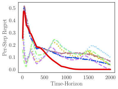
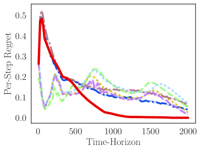
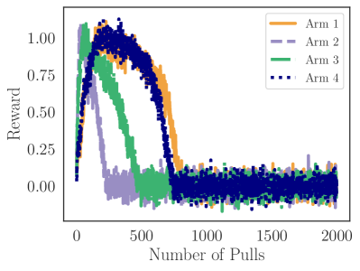
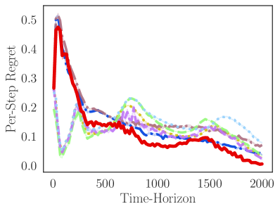
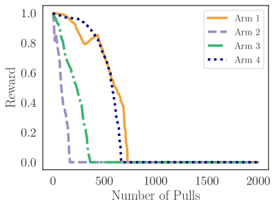
For monotonically increasing and concave reward functions we choose a set of synthetic functions that Heidari et al. (2016) use. We compare their algorithm, which is restricted to increasing, concave reward functions, to ours by plotting the per-step-regret of both algorithms. The results are shown in Figures 5, 5 and 7. Additionally we choose one of the reward function to test the robustness of the algorithms to noisy observations, shown in Figure 7. Figure 5 shows SPO perform comparably to Heidari et al. (2016)’s algorithm. In all other experiments SPO outperforms their algorithm significantly. Their algorithm fails especially when adding noise as in Figure 7. EXP3 and R-EXP3 perform poorly on all experiments, while D-UCB and SW-UCB work well in some of them, but fail in others.
D.2 Single-Peaked Reward Functions
Here we consider more synthetic single-peaked reward functions to evaluate SPO on, similar to Figure 1 in the main text. The experimental setup is as before with two reward functions and . We consider three sets of reward functions with different levels of Gaussian noise.
D.3 Gaussian Multi-armed Bandits
One might wonder if SPO can also be used for classical multi-armed bandits for which the rewards are drawn from a fixed distribution for each arm. Of course, one would expect SPO to perform worse in this situation than algorithms designed for the simple MAB problem. However, in some situations there might be little a priori information on the shape of the reward functions, and then it is beneficial to have an algorithm that can handle different situations such as increasing, decreasing or constant rewards.
To test whether SPO can handle simple MABs, we consider constant reward functions with Gaussian noise. This corresponds to a MAB setup where the reward of each arm is drawn from a Gaussian distribution with a fixed mean. We evaluate SPO on sets of arms with randomly sampled means, and compare it to UCB. Figure 11 shows that SPO can still find the optimal arm in this situation, but takes longer than UCB which is d.
D.4 FICO Dataset
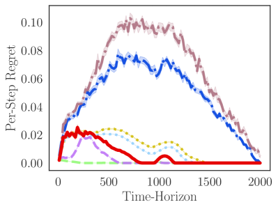
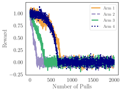
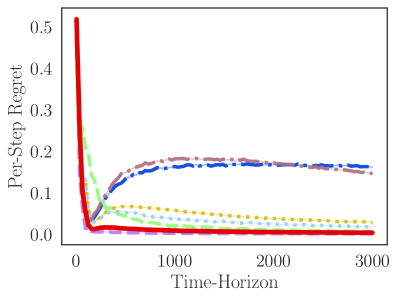
Figures 13 and 13 show additional results for our experiments using the FICO dataset.
Figure 13 shows the same results presented in the main paper, but for different simulated noise levels. The general observation that SPO outperforms all baselines holds across different levels of noise. As expected its advantage shrinks a bit for high noise levels.
In a separate experiment, we consider reward functions defined by the banks’s utility of giving a loan. We use the model by Liu et al. (2018), which assumes a utility of for a repaid loan and for a defaulted loan. In this case, the reward functions are decreasing almost everywhere. For monotonically decreasing reward functions Heidari et al. (2016) show that greedy approaches are optimal. This is also what we see in the results in Figure 13: both the greedy and the one-step-optimistic algorithm achieve no-policy-regret everywhere. However, our algorithm also achieves good performance and outperforms some of the other baselines significantly.
D.5 Simulated Recommender System
We randomly generate 3 instances of the simulated recommender system described in the main text. Figures 15, 15 and 16 show the reward functions and experimental results for different levels of simulated Gaussian noise. The results across all instances and noise levels are consistent with the results we report in the main paper, and they show that SPO outperforms all alternatives significantly except for very short time horizons.


 ) compared to the algorithm proposed by Heidari et al. (2016) for increasing rewards (
 ), EXP3 (
 ), R-EXP3 (
 ), D-UCB (
 ), and SW-UCB (
 ). The right-hand plots show the policies these algorithms choose in comparison to the optimal policy (
 ).
).
 ) compared to the algorithm proposed by Heidari et al. (2016) for increasing rewards (
 ), EXP3 (
 ), R-EXP3 (
 ), D-UCB (
 ), and SW-UCB (
 ). The right-hand plots show the policies these algorithms choose in comparison to the optimal policy (
 ).
).
 ) compared to the algorithm proposed by Heidari et al. (2016) for increasing rewards (
 ), EXP3 (
 ), R-EXP3 (
 ), D-UCB (
 ), and SW-UCB (
 ). The right-hand plots show the policies these algorithms choose in comparison to the optimal policy (
 ).
).
 ) compared to the algorithm proposed by Heidari et al. (2016) for increasing rewards (
 ), EXP3 (
 ), R-EXP3 (
 ), D-UCB (
 ), and SW-UCB (
 ). The right-hand plots show the policies these algorithms choose in comparison to the optimal policy (
 ).
).


 ) compared to UCB (
 ) on a Gaussian multi-armed bandit for different time horizons. We show the mean of the regret over 30 instances of MABs with 10 arms with means uniformly sampled between and .
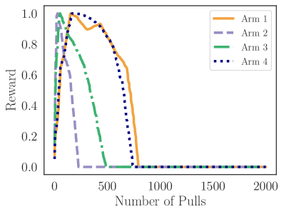
 ) compared to EXP3 (
 ), R-EXP3 (
 ), D-UCB (
 ), SW-UCB (
 ), a one-step-optimistic (
 ), and a greedy algorithm (
 ).
).
 ) compared to EXP3 (
 ), R-EXP3 (
 ), D-UCB (
 ), SW-UCB (
 ), a one-step-optimistic (
 ), and a greedy algorithm (
 ).
).
 ) compared to EXP3 (
 ), R-EXP3 (
 ), D-UCB (
 ), SW-UCB (
 ), a one-step-optimistic (
 ), and a greedy algorithm (
 ).
).
 ) compared to EXP3 (
 ), R-EXP3 (
 ), D-UCB (
 ), SW-UCB (
 ), a one-step-optimistic (
 ), and a greedy algorithm (
 ).
).
 ) compared to EXP3 (
 ), R-EXP3 (
 ), D-UCB (
 ), SW-UCB (
 ), a one-step-optimistic (
 ), and a greedy algorithm (
 ).
).