M5-brane Sources, Holography, and Argyres-Douglas Theories

Abstract

We initiate a study of the holographic duals of a class of four-dimensional $\mathcal{N}=2$ superconformal field theories that are engineered by wrapping M5-branes on a sphere with an irregular puncture. These notably include the strongly-coupled field theories of Argyres-Douglas type. Our solutions are obtained in 7d gauged supergravity, where they take the form of a warped product of $AdS_{5}$ and a “half-spindle.” The irregular puncture is modeled by a localized M5-brane source in the internal space of the gravity duals. Our solutions feature a realization of supersymmetry that is distinct from the usual topological twist, as well as an interesting Stückelberg mechanism involving the gauge field associated to a generator of the isometry algebra of the internal space. We check the proposed duality by computing the holographic central charge, the flavor symmetry central charge, and the dimensions of various supersymmetric probe M2-branes, and matching these with the dual Argyres-Douglas field theories. Furthermore, we compute the large-$N$ ’t Hooft anomalies of the field theories using anomaly inflow methods in M-theory, and find perfect agreement with the proposed duality.

1 Introduction

The Argyres-Douglas (AD) field theories have particular significance among four-dimensional $\mathcal{N}=2$ superconformal field theories (SCFTs). As in the original such theory discovered by Argyres and Douglas in Argyres:1995jj , many of these SCFTs appear at special singular points on the moduli space of $\mathcal{N}=2$ gauge theories where mutually non-local dyons simultaneously become massless Argyres:1995xn ; Eguchi:1996vu . Such phenomena cannot be captured by a Lagrangian in the traditional sense, and thus these theories are intrinsically strongly coupled. Nonetheless, the existence of an interacting superconformal fixed point has been convincingly argued from both field theoretic and string theoretic perspectives.

Several features of the Argyres-Douglas theories set them apart. A dramatic example is that they possess relevant chiral operators in their spectrum with fractional scaling dimensions. Among all unitary interacting $\mathcal{N}=2$ SCFTs, the theory with smallest $c$-central charge is the original AD theory with one relevant chiral ring generator of dimension $\frac{6}{5}$, and in this sense the “minimal” ${\cal N}=2$ SCFT is of Argyres-Douglas type Liendo:2015ofa .

Argyres-Douglas SCFTs also appear in the low-energy limit of various string theory configurations via geometric engineering. One such realization involves compactifying the 6d $\mathcal{N}=(2,0)$ SCFTs of $\mathfrak{g}=$ADE type on a punctured sphere, which for $\mathfrak{g}=A_{N-1}$ corresponds to $N$ M5-branes wrapped on the sphere. An infinite class of four-dimensional conformal field theories with varying amounts of supersymmetry can be obtained by compactifying the (2,0) theories on a punctured Riemann surface, while employing a topological twist to preserve supersymmetry in four dimensions, beginning with the $\mathcal{N}=2$ constructions in Witten:1997sc ; Gaiotto:2009we ; Gaiotto:2009hg . A large subset of Argyres-Douglas theories can be thus obtained in the very special case that the Riemann surface is a sphere with a puncture of irregular, rather than regular, type Bonelli:2011aa ; Xie:2012hs ; Wang:2015mra (also see Gaiotto:2009hg ; Witten:2007td ). While the holographic duals of a large class of 4d $\mathcal{N}=2$ SCFTs in geometric engineering with regular punctures are known Gaiotto:2009gz , until now the gravity duals of 4d field theories from irregular punctures have remained mysterious.

The realization of Argyres-Douglas theories via M5-branes wrapped on spheres with irregular punctures offers the prospect of studying their properties in holography. In this paper we present the first gravity duals of AD theories in M-theory, and provide a new perspective on both the geometry of the irregular puncture and the curious field theoretic properties of these SCFTs. An important motivation to this work has been the recent work on branes wrapping spindle geometries Ferrero:2020laf ; Ferrero:2020twa as a novel way of preserving supersymmetry beyond the paradigm of the topological twist in supergravity Maldacena:2000mw . Our construction will provide yet another way of preserving supersymmetry, by wrapping branes on a disk with a nontrivial $U(1)$ holonomy at the boundary. Our setup can be thought of as M5-branes wrapping a “half-spindle”.

A distinctive feature of our 11d solutions is the presence of localized M5-brane sources in the internal space. These appear as singularities in the low-energy supergravity approximation, but correspond to well-defined objects in the full M-theory. As demonstrated in several examples Brandhuber:1999np ; Apruzzi:2013yva ; Gaiotto:2014lca ; Apruzzi:2015wna ; DHoker:2016ujz ; DHoker:2017mds ; Bah:2017wxp ; Bah:2018lyv , brane sources are useful ingredients in holography. In particular, they provide an avenue to realizing arbitrary flavor symmetries. In our solutions the M5-brane source is instrumental, and is in fact dual to the irregular puncture on the sphere. This novel connection between irregular punctures and sources in supergravity paves the way to further investigations and generalizations to other brane constructions.

Another peculiar property of our solutions is related to the interplay between the isometry algebra of the internal space and the algebra of global zero-form symmetries in the SCFT. In particular, we identify a $U(1)$ isometry generator that is not mapped to a generator of a continuous $U(1)$ global zero-form symmetry of the dual field theory. Indeed, the would-be massless $U(1)$ gauge field associated to this isometry generator is actually massive in the $AdS_{5}$ low-energy effective action, by virtue of a novel Stückelberg mechanism involving an axion field originating from the expansion of the M-theory 3-form. The interplay between the background $G_{4}$-flux supporting the holographic solution and the isometry group of the internal space can be elegantly described in the language of equivariant cohomology. Our physical analysis in terms of a Stückelberg mechanism detects an obstruction to finding a closed equivariant completion of $G_{4}$—and provides a recipe to overcome it.

The rest of this paper is organized as follows. In section 2 we present a new class of $AdS_{5}$ solutions in 11d supergravity that preserve ${\cal N}=2$ superconformal symmetry. We first describe the solutions in 7d $U(1)^{2}$ gauged supergravity, and then give their uplift on $S^{4}$ to eleven dimensions. The solutions feature an M5-brane source, and their flux configuration is encoded by three positive integers. We compute the holographic central charge, as well as the charges of various supersymmetric probe M2-branes wrapping two-cycles in the internal space.

In section 3 we use the machinery of anomaly inflow to extract the global symmetries and ’t Hooft anomalies of the SCFTs dual to the aforementioned supergravity solutions. We verify that the central charge thus computed is compatible with the holographic central charge, and additionally compute the flavor central charge. An important ingredient in the matching of the global symmetries is a Stückelberg mechanism, in which one $U(1)$ generator of the isometry algebra of the internal space is spontaneously broken.

In section 4 we describe the proposed 4d ${\cal N}=2$ field theories dual to our supergravity solutions, and perform tests of the holographic duality. The field theories are of Argyres-Douglas type, and arise from $N$ M5-branes wrapped on a sphere with one irregular puncture and one regular puncture. We test the duality by matching the ${\cal N}=2$ R-symmetry generators, the large-$N$ central charge, the flavor central charge associated to the regular puncture, the rank of the flavor symmetry, and the field theory operators dual to M2-brane probes.

Finally, several appendices elaborate on derivations and ideas used in the main text. Appendix A provides a full derivation of the 7d gauged supergravity solutions. Appendix B casts the uplifted 11d solutions into canonical $\mathcal{N}=2$ form. Appendix C collects useful formulae on the ’t Hooft anomalies of 4d ${\cal N}=2$ SCFTs. Appendices D and E serve as select reviews of the literature on Argyres-Douglas theories: appendix D gives an overview of the landscape of four-dimensional field theories of Argyres-Douglas type, while appendix E reviews the dual quiver Lagrangian description found in Agarwal:2017roi ; Benvenuti:2017bpg of a subclass of the AD theories dual to our supergravity solutions.

A brief summary of some results of the supergravity solutions and checks of the proposed duality were first reported in Bah:2021mzw .

2 Supergravity Solutions

This section is devoted to a discussion of a new class of 11d supergravity $AdS_{5}$ solutions. They are first obtained in 7d gauged supergravity and then uplifted to eleven dimensions.

2.1 Solutions in 7d Supergravity

The reduction of 11d supergravity on $S^{4}$ yields the 7d $\mathcal{N}=4$ $SO(5)$ gauged supergravity of Pernici:1984xx . In this work we consider a further truncation to the Cartan subgroup $U(1)^{2}$ of $SO(5)$. We follow the notation and conventions of Liu:1999ai . The bosonic field content of the $U(1)^{2}$ truncated model consists of the 7d metric $g_{\mu\nu}$, two real scalars $\lambda_{1}$, $\lambda_{2}$, two $U(1)$ gauge fields $A^{(1)}_{\mu}$, $A^{(2)}_{\mu}$, and a real 3-form potential $C_{\mu\nu\rho}$. (The indices $\mu$, $\nu$, …are curved 7d spacetime indices.) The equations of motion and BPS equations for this supergravity model are recorded in appendix A.1. The mass scale of the model is denoted $m$. In our conventions, the $AdS_{7}$ vacuum solution has radius $L_{AdS_{7}}=2/m$. The gauge coupling of the model is denoted $g$, and supersymmetry relates it to $m$ as $g=2\,m$.

As derived in appendix A, the following bosonic field configurations preserve 4d $\mathcal{N}=2$ superconformal symmetry and solve all equations of motion. The 7d metric is given by

$$m^{2}\,ds_{7}^{2} =\frac{2\,B\,w^{3/5}}{\sqrt{\kappa\,(1-w^{2})}}\,\bigg{[}ds^{2}(AdS_{5})+ds^{2}(\Sigma)\bigg{]}\ ,$$

$$ds^{2}(\Sigma) =\frac{dw^{2}}{2\,w\,h(w)\,[\kappa\,(1-w^{2})]^{3/2}}+\frac{\mathcal{C}^{2}\,h(w)\,dz^{2}}{B}\ .$$ (2.1)

Here $ds^{2}(AdS_{5})$ is the unit-radius metric in $AdS_{5}$, $w$ is an interval coordinate whose range is discussed below, $z$ is an angular coordinate, $B$ is a positive constant, $\mathcal{C}$ is a real constant, $\kappa\in\{1,-1\}$ is a sign, and the function $h(w)$ is given by

$$h(w)=B-2\,w\,\sqrt{\kappa\,(1-w^{2})}\ .$$ (2.2)

The scalar fields $\lambda_{1}$, $\lambda_{2}$ depend on the coordinate $w$ only and are given as

$$\lambda_{1}=\frac{3}{5}\,\log w\ ,\qquad\lambda_{2}=-\frac{2}{5}\,\log w\ .$$ (2.3)

The gauge field $A^{(1)}$ has field strength $F^{(1)}=dA^{(1)}$ given by

$$F^{(1)}=-2\,m^{-1}\,\mathcal{C}\,w\,dw\wedge dz\ ,$$ (2.4)

while the other gauge field $A^{(2)}$ and the 3-form potential $C$ are set to zero. We observe that the angular coordinate $z$ enters the 7d metric and the field strength $F^{(1)}$ always in the combination $\mathcal{C}\,dz$. Without loss of generality we can then assign periodicity $2\pi$ to the coordinate $z$.

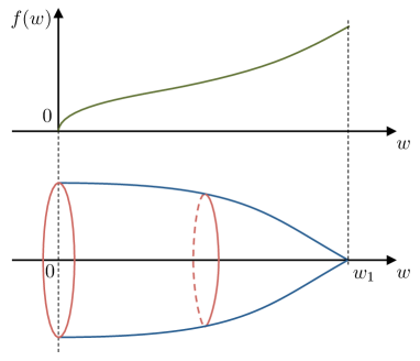
Figure 1: A schematic depiction of the internal geometry for the choice of parameters and range of the $w$ coordinate specified in (2.5). The $z$ circle is fibered over the $w$ interval to yield $\Sigma$ with metric $ds^{2}(\Sigma)$ in (2.1). $\Sigma$ has the topology of a disk with a $\mathbb{Z}_{\ell}$ orbifold singularity at the center. We also depict the qualitative behavior of the $AdS_{5}$ warp function $f(w)=2\,B\,w^{3/5}/\sqrt{1-w^{2}}$.

The range of the coordinate $w$ is constrained by requiring that $\lambda_{1}$, $\lambda_{2}$ be real and the 7d metric positive-definite. Depending on the parameters $\kappa$ and $B$ there are various cases, listed in appendix A.5. The case of main interest for this paper is

$$\kappa=1\ ,\qquad 0<B<1\ ,\qquad 0<w<w_{1}:=\tfrac{1}{2}\,\Big{(}\sqrt{1+B}-\sqrt{1-B}\Big{)}\ .$$ (2.5)

Let us describe the behavior of the metric near the two endpoints $w=w_{1}$ and $w=0$ in turn.

In the vicinity of $w=w_{1}$, the $AdS_{5}$ warp factor is smooth, and the $z$ circle shrinks. (The function $h$ has a simple zero at $w=w_{1}$.) By tuning the constant parameter $\mathcal{C}$ we can ensure that $z$ shrinks smoothly. More generally, if we impose

$$|\mathcal{C}|=\frac{1}{\ell\,\sqrt{1-B^{2}}}\ ,\qquad\ell=1,2,3,\dots\ ,$$ (2.6)

the shrinking of the $z$ circle gives an orbifold point $\mathbb{R}^{2}/\mathbb{Z}_{\ell}$. For more details, see appendix A.5. Near $w=0$ the $AdS_{5}$ warp factor vanishes and the 7d metric becomes conformal to the direct product of $AdS_{5}$ and a cylinder. This can be seen setting $w=r^{2}$ and observing that

$$m^{2}\,ds^{2}_{7}\approx 2\,B\,r^{6/5}\,\Big{[}ds^{2}(AdS_{5})+2\,B^{-1}\,dr^{2}+\mathcal{C}^{2}\,dz^{2}\Big{]}\ ,\qquad r\rightarrow 0^{+}\ .$$ (2.7)

The locus $r=0$ is a curvature singularity of the total 7d metric. Figure 1 gives a schematic depiction of $\Sigma$ and the $AdS_{5}$ warp factor.

The space $\Sigma$, equipped with the metric $ds^{2}(\Sigma)$ as in (2.1), has the topology of a disk, with the origin at $w=w_{1}$ and the boundary at $w=0$. Indeed, the $z$ circle does not shrink at $w=0$ in the metric $ds^{2}(\Sigma)$. As observed above, we have a $\mathbb{Z}_{\ell}$ orbifold singularity at the origin of the disk $\Sigma$. There exists a gauge choice such that $A^{(1)}$ is well-defined near $w=w_{1}$,

$$A^{(1)}=-m^{-1}\,\mathcal{C}\,(w^{2}-w_{1}^{2})\,dz\ .$$ (2.8)

Notice that we have fixed the ambiguity in $A^{(1)}$ by a shift by a constant times $dz$ by requiring that the prefactor of $dz$ vanishes at $w=w_{1}$. In this gauge, $A^{(1)}$ is globally defined on the disk $\Sigma$. In appendix A.4 we verify that the Killing spinor on $\Sigma$ is also well-defined near $w=w_{1}$, and is therefore globally defined on the disk $\Sigma$.

A brief digression about the normalization of $A^{(1)}$ is necessary. To find the natural normalization, we observe that $A^{(1)}$ is identified with the $ab=12$ component of the field strength $F^{ab}$ of the full $SO(5)$ gauged supergravity model (the indices $a$, $b=1,\dots,5$ are vector indices of $SO(5)$). In the conventions of this paper—see also Pernici:1984xx ; Liu:1999ai —the expression for $F^{ab}$ is $F^{ab}=dA^{ab}+g\,A^{ac}\wedge A_{c}{}^{b}$, where $g=2m$ is the gauge coupling constant of the supergravity theory. It is natural to rescale $A^{ab}$ to eliminate the factor $g$ between the linear and quadratic terms in the field strength: we set

$$A^{ab}=\frac{1}{2m}\,\mathsf{A}^{ab}\ ,$$ (2.9)

so that the field strength of $\mathsf{A}^{ab}$ is $\mathsf{F}^{ab}=d\mathsf{A}^{ab}+\mathsf{A}^{ac}\wedge\mathsf{A}_{c}{}^{b}$. The rescaling of $A^{ab}$ induces an analogous rescaling of $A^{(1)}$,

$$A^{(1)}=\frac{1}{2m}\,\mathsf{A}^{(1)}\ .$$ (2.10)

Since in the gauge (2.8) $\mathsf{A}^{(1)}$ is globally defined on the disk $\Sigma$, the flux of the field strength $\mathsf{F}^{(1)}=d\mathsf{A}^{(1)}$ through $\Sigma$ equals minus the holonomy of $\mathsf{A}^{(1)}$ along the boundary at $w=0$,

$${\rm hol}_{\partial\Sigma}(\mathsf{A}^{(1)}):=\oint_{w=0}\frac{\mathsf{A}^{(1)}}{2\pi}=-\int_{\Sigma}\frac{\mathsf{F}^{(1)}}{2\pi}=2\,\mathcal{C}\,w_{1}^{2}=\mathcal{C}\,(1-\sqrt{1-B^{2}})\ .$$ (2.11)

We assign positive orientation to $dw\wedge dz$, with $w$ increasing from $0$ to $w_{1}$.

The parameters $B$, $\mathcal{C}$ in the 7d solution can be expressed in terms of the integer $\ell$ and the holonomy ${\rm hol}_{\partial\Sigma}(\mathsf{A}^{(1)})$,

$$\mathcal{C}={\rm hol}_{\partial\Sigma}(\mathsf{A}^{(1)})+\frac{1}{\ell}\ ,\qquad\sqrt{1-B^{2}}=\frac{1}{1+\ell\,{\rm hol}_{\partial\Sigma}(\mathsf{A}^{(1)})}\ .$$ (2.12)

We have anticipated that $\mathcal{C}$ is positive, which will be verified when we perform the uplift to eleven dimensions in section 2.3. We think of $\ell$ and ${\rm hol}_{\partial\Sigma}(\mathsf{A}^{(1)})$ as the geometric and gauge-theoretic input data that specify the solution. At this stage ${\rm hol}_{\partial\Sigma}(\mathsf{A}^{(1)})$ is an arbitrary real quantity. We will see that, in the uplifted solutions, it is identified with the ratio of two integer $G_{4}$-flux quanta.

Let us compute the Euler characteristic $\chi(\Sigma)$ of $\Sigma$ from the line element $ds^{2}(\Sigma)$ in (2.1) using the Gauss-Bonnet theorem, following similar computations in Ferrero:2020laf ; Ferrero:2020twa . A potential contribution originates from the boundary of $\Sigma$. One verifies, however, that the boundary at $w=0$ is a geodetic in the metric $ds^{2}(\Sigma)$, and thus has vanishing geodetic curvature. As a result, the only contribution to $\chi(\Sigma)$ originates from integrating the Ricci scalar of $ds^{2}(\Sigma)$ against the volume form of the metric $ds^{2}(\Sigma)$,

$$\chi(\Sigma)=\frac{1}{4\pi}\,\int_{\Sigma}R_{\Sigma}\,{\rm vol}_{\Sigma}=\frac{\sqrt{2}\,\sqrt{w}_{1}\,\mathcal{C}\,(1-2w_{1}^{2})\,(1-w_{1}^{2})^{1/4}}{\sqrt{B}}=\mathcal{C}\,\sqrt{1-B^{2}}=\frac{1}{\ell}\ .$$ (2.13)

This is the expected result for a disk in $\mathbb{R}^{2}/\mathbb{Z}_{\ell}$ centered at the origin.

Our 7d solutions can be compared to the spindle solutions of Ferrero:2020laf ; Ferrero:2020twa ; Hosseini:2021fge ; Boido:2021szx ; Ferrero:2021wvk . As in those references, the 2d space $\Sigma$ is not equipped with a constant curvature metric. The gauge field $A^{(1)}$ does not cancel the spin connection on $\Sigma$, and the Killing spinor has a non-trivial profile in the $w$ direction (its explicit expression is recorded in (A.68)). These features signal that supersymmetry is realized in a way that deviates from the standard topological twist paradigm. In contrast to Ferrero:2020laf ; Ferrero:2020twa ; Hosseini:2021fge ; Boido:2021szx ; Ferrero:2021wvk , however, our internal space $\Sigma$ has the topology of a disk, with a non-trivial holonomy of the gauge field $A^{(1)}$ along its boundary. This is qualitatively different from the spindle geometries. Our $\Sigma$ may be intuitively thought of as a “half spindle” and leads to a new way of realizing supersymmetry.

2.2 Uplift to Eleven Dimensions

The uplift on $S^{4}$ of solutions to the 7d $U(1)^{2}$ gauged supergravity model considered above has been analyzed in Cvetic:1999xp . To perform the uplift, we find it convenient to make use of the formulae in Nastase:1999kf . It is useful to keep in mind that the authors of Nastase:1999kf set implicitly $m=1$; it is straightforward to restore factors of $m$ in their expressions. The 11d metric is given as

$$ds_{11}^{2}=(T_{ab}\,Y^{a}\,Y^{b})^{1/3}\,ds^{2}_{7}+m^{-2}\,(T_{ab}\,Y^{a}\,Y^{b})^{-2/3}\,(T^{-1})_{ab}\,DY^{a}\,DY^{b}\ .$$ (2.14)

The indices $a,b=1,\dots,5$ are $SO(5)$ indices and are raised/lowered with $\delta$. The quantities $Y^{a}$ are constrained coordinates on $S^{4}$, satisfying $Y^{a}\,Y_{a}=1$. The symmetric, unimodular matrix $T_{ab}$ is constructed with the scalar fields $\lambda_{1}$, $\lambda_{2}$ as

$$T_{ab}={\rm diag}(e^{2\lambda_{1}},e^{2\lambda_{1}},e^{2\lambda_{2}},e^{2\lambda_{2}},e^{-4\lambda_{1}-4\lambda_{2}})\ .$$ (2.15)

The 1-form $DY^{a}$ is defined as

$$DY^{a}=dY^{a}+g\,A^{ab}\,Y_{b}\ ,$$ (2.16)

(recall that $g=2\,m$) where $A^{[ab]}$ is an $SO(5)$ connection with legs on 7d spacetime. Its only non-zero components are

$$A^{12}=A^{(1)}\ ,\qquad A^{34}=A^{(2)}\ .$$ (2.17)

The expression for $G_{4}$ is

$$G_{4}=\frac{1}{8\,m^{3}}\,\epsilon_{abcde}\,\bigg{[} \frac{4}{3}\,DY^{a}\,DY^{b}\,DY^{c}\,DY^{d}\,Y^{e}-\frac{1}{3}\,DY^{a}\,DY^{b}\,DY^{c}\,DY^{d}\,\widetilde{Y}^{e}$$

$$+2\,g\,F^{ab}\,DY^{c}\,DY^{d}\,\widetilde{Y}^{e}+g^{2}\,F^{ab}\,F^{cd}\,Y^{e}\bigg{]}+dC_{3}\ ,$$ (2.18)

where $C_{3}$ is the 3-form potential of the 7d supergravity model. We have suppressed wedge products and we have used the quantities

$$F^{ab}=dA^{ab}+g\,A^{ac}\,A_{c}{}^{b}\ ,\qquad\widetilde{Y}^{a}:=\frac{T^{ab}\,Y_{b}}{T_{cd}\,Y^{c}\,Y^{d}}\ .$$ (2.19)

We parametrize the constrained coordinates $Y^{a}$ as

$$Y^{1}=\sqrt{1-\mu^{2}}\,\cos\phi\ ,\qquad Y^{2}=\sqrt{1-\mu^{2}}\,\sin\phi\ ,\qquad Y^{3,4,5}=\mu\,\hat{y}^{1,2,3}\ ,$$ (2.20)

where the three real coordinates $\hat{y}^{1,2,3}$ are subject to the constraint $(\hat{y}^{1})^{2}+(\hat{y}^{2})^{2}+(\hat{y}^{3})^{2}=1$ and thus parametrize an $S^{2}\subset\mathbb{R}^{3}$. The coordinate $\mu$ has range $[0,1]$ and the angular coordinate $\phi$ has periodicity $2\pi$. Using the 7d line element (2.1), the 7d scalar fields (2.3), and the 7d gauge field (2.4), the uplift formula (2.14) yields

$$m^{2}\,ds^{2}_{11} =\frac{2\,B\,w^{1/3}\,\mathcal{H}(w,\mu)^{1/3}}{\sqrt{\kappa\,(1-w^{2})}}\,\bigg{[}ds^{2}(AdS_{5})+\frac{dw^{2}}{2\,w\,h(w)\,[\kappa\,(1-w^{2})]^{3/2}}+\frac{\mathcal{C}^{2}\,h(w)\,dz^{2}}{B}$$

$$+\frac{\sqrt{\kappa\,(1-w^{2})}}{2\,B}\,\bigg{(}\frac{d\mu^{2}}{w\,(1-\mu^{2})}+\frac{(1-\mu^{2})\,D\phi^{2}}{w\,\mathcal{H}(w,\mu)}\,+\frac{w\,\mu^{2}\,ds^{2}(S^{2})}{\mathcal{H}(w,\mu)}\bigg{)}\bigg{]}\ .$$ (2.21)

We have introduced the notation

$$\mathcal{H}(w,\mu)=\mu^{2}+w^{2}\,(1-\mu^{2})\ .$$ (2.22)

The function $h(w)$ was defined in (2.2). The quantity $ds^{2}(S^{2})$ is the metric on the round unit 2-sphere parametrized by $\hat{y}^{1,2,3}$, while the 1-form $D\phi$ is given as

$$D\phi=d\phi+\mathcal{C}\,(2\,w^{2}-1)\,dz\ .$$ (2.23)

The expression for $G_{4}$ that follows from (2.2) is

$$G_{4}=-\frac{1}{m^{3}}\,{\rm vol}_{S^{2}}\,d\bigg{[}\frac{\mu^{3}}{\mu^{2}+w^{2}\,(1-\mu^{2})}\,D\phi\bigg{]}\ ,$$ (2.24)

where ${\rm vol}_{S^{2}}$ is the volume form on the 2-sphere of unit radius.

2.3 Internal Geometry and Flux Quantization

For the rest of this section we specialize to the choice of parameters and range for $w$ given in (2.5). The other possibilities discussed in appendix A.5 may also be uplifted to eleven dimensions and discussed in a similar fashion.

2.3.1 Geometry of the Internal Space

The 6d internal space in the 11d line element (2.2) can be regarded as an $S^{1}_{\phi}\times S^{1}_{z}\times S^{2}$ fibration over the 2d base space $B_{2}$ parametrized by $w$ and $\mu$, which is the rectangle $[0,w_{1}]\times[0,1]$, see Figure 2. Let us describe in greater detail the features of the internal geometry near the following three regions of the boundary of the rectangle $B_{2}$:

• Region I: a neighborhood of the side $\mathsf{P}_{1}\mathsf{P}_{2}$ (depicted in green).

• Region II: a neighborhood of the union of the sides $\mathsf{P}_{2}\mathsf{P}_{3}$ and $\mathsf{P}_{3}\mathsf{P}_{4}$ (depicted in blue).

• Region III: a neighborhood of the side $\mathsf{P}_{1}\mathsf{P}_{4}$ (depicted in red).

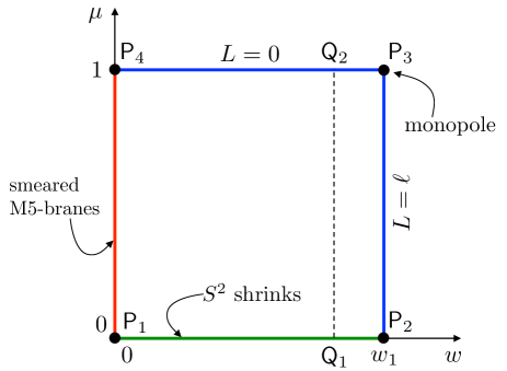
Figure 2: The internal space in the 11d solution is an $S^{1}_{\phi}\times S^{1}_{z}\times S^{2}$ fibration over the rectangle in the $(w,\mu)$ plane delimited by the points $\mathsf{P}_{1}$, $\mathsf{P}_{2}$, $\mathsf{P}_{3}$, $\mathsf{P}_{4}$. We indicate the constant value of the function $L$ in the line element (2.25) on the sides $\mathsf{P}_{2}\mathsf{P}_{3}$ and $\mathsf{P}_{3}\mathsf{P}_{4}$. The point $\mathsf{P}_{3}$ is the location of a monopole of charge $\ell$ for the $Dz$ fibration in (2.25). The warp factor vanishes along the side $\mathsf{P}_{1}\mathsf{P}_{4}$. The geometry in this region is interpreted in terms of smeared M5-branes. We also include the segment $\mathsf{Q}_{1}\mathsf{Q}_{2}$ which is used in section 2.3.2 in the discussion of $G_{4}$-flux quantization.

Geometry of Region I.

As we approach a point along the $\{\mu=0\}$ side of the rectangle $B_{2}$, at generic $w\in(0,w_{1})$, the $S^{2}$ shrinks smoothly, capping off the internal space. Both Killing vector fields $\partial_{z}$ and $\partial_{\phi}$ have a finite norm as we approach $\mu=0$.

Geometry of Region II: Regular Puncture.

To describe the geometry of this region we make use of the angular coordinates $\phi$, $z$, but we break up the 1-form $D\phi$ and complete instead the $dz$ square. The resulting line element takes the form

$$ds^{2}_{11} =\frac{2\,B\,w^{1/3}\,\mathcal{H}^{1/3}}{m^{2}\,\sqrt{1-w^{2}}}\,\bigg{[}ds^{2}(AdS_{5})+\frac{\sqrt{1-w^{2}}\,\mu^{2}\,w\,ds^{2}(S^{2})}{2\,B\,\mathcal{H}}$$ (2.25)

$$+\frac{dw^{2}}{2\,h\,w\,(1-w^{2})^{3/2}}+\frac{\sqrt{1-w^{2}}\,d\mu^{2}}{2\,B\,w\,(1-\mu^{2})}+R_{\phi}^{2}\,d\phi^{2}+R_{z}^{2}\,Dz^{2}\bigg{]}\ ,\qquad Dz=dz-L\,d\phi\ .$$

The function $h$ is defined in (2.2), while $\mathcal{H}$ is defined in (2.22). The metric functions $R_{\phi}^{2}$, $R_{z}^{2}$ and the function $L$ inside $Dz$ are given as

$$R_{\phi}^{2} =\frac{h\,(1-\mu^{2})\,\sqrt{1-w^{2}}}{B\,\Big{[}2\,h\,w\,\mathcal{H}+(2w^{2}-1)^{2}\,(1-\mu^{2})\,\sqrt{1-w^{2}}\Big{]}}\ ,$$

$$R_{z}^{2} =\frac{2\,h\,w\,\mathcal{H}+(2w^{2}-1)^{2}\,(1-\mu^{2})\,\sqrt{1-w^{2}}}{2\,B\,w\,\mathcal{H}}\,\mathcal{C}^{2}\ ,$$

$$L =\frac{-(2w^{2}-1)\,(1-\mu^{2})\,\sqrt{1-w^{2}}}{\mathcal{C}\,\Big{[}2\,h\,w\,\mathcal{H}+(2w^{2}-1)^{2}\,(1-\mu^{2})\,\sqrt{1-w^{2}}\Big{]}}\ .$$ (2.26)

We are describing the internal space in terms of $S^{2}$ and the 4d space spanned by $w$, $\mu$, $\phi$, $z$. The latter is an $S^{1}_{z}$ fibration over the 3d space spanned by $w$, $\mu$, $\phi$. This description is modeled after Gaiotto:2009gz and the local geometries that describe regular punctures for M5-branes wrapped on a Riemann surface Bah:2018jrv ; Bah:2019jts . The $Dz$ fibration over $w$, $\mu$, $\phi$ is a convenient device to keep track of the two different linear combinations of the Killing vectors $\partial_{\phi}$, $\partial_{z}$ whose norms go to zero on the two sides $\{w=w_{1}\}$ and $\{\mu=1\}$ of the rectangle $B_{2}$.

We observe that $R_{\phi}^{2}$ is the radius squared of the $\phi$ circle in the 3d base, and that it goes to zero both along $\mu=1$ and $w=w_{1}$. More precisely, one can verify that

$$\mu =1-\varrho^{2}\ , \varrho \rightarrow 0^{+}\ , \frac{\sqrt{1-w^{2}}\,d\mu^{2}}{2\,B\,w\,(1-\mu^{2})}+R_{\phi}^{2}\,d\phi^{2} \approx\frac{\sqrt{1-w^{2}}}{2\,B\,w}\,(d\varrho^{2}+\varrho^{2}\,d\phi^{2})\ ,$$ (2.27)

$$w =w_{1}-\varrho^{2}\ , \varrho \rightarrow 0^{+}\ , \frac{\sqrt{1-w^{2}}\,dw^{2}}{2\,h\,w\,(1-w^{2})^{2}}+R_{\phi}^{2}\,d\phi^{2} \approx\frac{2\,(1-w_{1}^{2})^{-3/2}}{w_{1}\,(-h^{\prime}(w_{1}))}\,(d\varrho^{2}+\varrho^{2}\,d\phi^{2})\ .$$

These relations demonstrate that, in the 3d base of the $Dz$ fibration, the shrinking of the $\phi$ circle is smooth. The 3d base space is thus locally $\mathbb{R}^{3}$ in the vicinity of the boundary of $B_{2}$, with $\phi$ playing the role of an azimuthal angle in cylindrical coordinates. The radius squared $R^{2}_{z}$ of the $z$ circle, on the other hand, is only zero at the corner $(w,\mu)=(w_{1},1)$.

The function $L(w,\mu)$ is piecewise constant along the sides $\{w=w_{1}\}$ and $\{\mu=1\}$ of the rectangle $B_{2}$. More precisely, one finds

$$L(w,1)=0\ ,\qquad L(w_{1},\mu)=\frac{1}{\mathcal{C}\,\sqrt{1-B^{2}}}\ .$$ (2.28)

The jump in $L$ at the corner $(w,\mu)=(w_{1},1)$ signals the presence of a monopole source for the $Dz$ fibration. The monopole charge must be an integer. We find it convenient to adopt the same orientation conventions as in the discussion of the local puncture geometries of Bah:2019jts . In particular, the function $L$ is non-negative and decreasing as we move along the axis of the $\mathbb{R}^{3}$ fiber (spanned by $w$, $\mu$, $\phi$), starting from the point where the $S^{2}$ shrinks (point $\mathsf{P}_{2}$ in Figure 2) and moving upwards towards $\mathsf{P}_{3}$ and then past the monopole towards $\mathsf{P}_{4}$. These considerations imply that $\mathcal{C}$ is positive, so that

$$\frac{1}{\mathcal{C}\,\sqrt{1-B^{2}}}=\ell\ ,\qquad\ell=1,2,3,\dots\ .$$ (2.29)

The integral quantization of the monopole charge can also be confirmed by a local analysis of the metric near the corner $(w,\mu)=(w_{1},1)$. More precisely, we trade $w$, $\mu$ for coordinates $R>0$ and $\theta\in[0,\pi]$ defined via

$$\mu=1-\frac{w_{1}^{2/3}}{2}\,R^{2}\,\cos^{2}\frac{\theta}{2}\ ,\qquad w=w_{1}-\frac{(1-B^{2})^{1/2}\,w_{1}^{5/3}\,(1-w_{1}^{2})^{2}}{B^{2}}\,R^{2}\,\sin^{2}\frac{\theta}{2}\ .$$ (2.30)

In the limit $R\rightarrow 0$, the 11d line element reads

$$m^{2}\,ds^{2}_{11} \approx 4\,w_{1}^{4/3}\,ds^{2}(AdS_{5})+w_{1}^{4/3}\,ds^{2}(S^{2})$$

$$+dR^{2}+R^{2}\,\bigg{\{}\frac{d\theta^{2}+\sin^{2}\theta\,d\phi^{2}}{4}+\mathcal{C}^{2}\,(1-B^{2})\,\bigg{[}dz-\frac{1+\cos\theta}{2\,\mathcal{C}\,\sqrt{1-B^{2}}}\,d\phi\bigg{]}^{2}\bigg{\}}\ .$$ (2.31)

If $\mathcal{C}\,\sqrt{1-B^{2}}=1$, the line element in curly brackets in the second line is a round $S^{3}$ presented as a standard Hopf fibration. The Hopf fiber is parametrized by $z$ with period $2\pi$, while the Hopf base is spanned by $\theta\in[0,\pi]$ and $\phi$ with periodicity $2\pi$. More generally, we can allow the quantity $\mathcal{C}\,\sqrt{1-B^{2}}$ to be $1/\ell$ for any positive integer $\ell$, as indicated in (2.29). The quantity in curly brackets is then the metric on $S^{3}/\mathbb{Z}_{\ell}$. When the latter is combined with the radial direction $R$, we obtain the metric on $\mathbb{R}^{4}/\mathbb{Z}_{\ell}$. Thus, for $\ell>1$ the geometry in Region II has an orbifold singularity at the location of the monopole, and is smooth elsewhere. We have demonstrated that the relation (2.6) in the 7d gauged supergravity solution is reinterpreted in the uplifted 11d solution as the quantization of a monopole charge.

Geometry of Region III: Smeared M5-branes.

This region requires special care because the warp factor in front of the $AdS_{5}$ metric goes to zero as $w$ approaches 0. The 11d line element can be approximated at small $w$ as

$$m^{2}\,ds^{2}_{11} \approx w^{1/3}\,\bigg{[}2\,B\,\mu^{2/3}\,ds^{2}(AdS_{5})+2\,\mathcal{C}^{2}\,B\,\mu^{2/3}\,dz^{2}\bigg{]}$$

$$+w^{-2/3}\,\bigg{[}\mu^{2/3}\,\Big{(}dw^{2}+w^{2}\,ds^{2}(S^{2})\Big{)}+\frac{\mu^{2/3}}{1-\mu^{2}}\,d\mu^{2}+\mu^{-4/3}\,(1-\mu^{2})\,D\phi^{2}\bigg{]}\ .$$ (2.32)

This line element is interpreted as originating from smeared M5-brane sources. More precisely, the M5-branes are:

• extended along the $AdS_{5}$ and $z$ directions;

• localized at the origin of the $\mathbb{R}^{3}$ parametrized by $S^{2}$ and $w$, $ds^{2}(\mathbb{R}^{3})=dw^{2}+w^{2}\,ds^{2}(S^{2})$;

• smeared along the $\mu$ and $\phi$ directions.

After smearing, the branes are effectively real codimension-3 objects. Notice that $w$ is identified with the radial coordinate away from the smeared branes. The relevant harmonic function for a real codimension-3 problem is $H\propto 1/w$. As appropriate for an M5-brane solution, we find a prefactor $H^{-1/3}$ in front of the six directions along which the M5-branes extend, while we find a factor $H^{2/3}$ in front of the five directions in which the branes are localized or smeared.

We can confirm the presence of an M5-brane source from the expression of $G_{4}$ near $w=0$,

$$G_{4}=-\frac{{\rm vol}_{S^{2}}\wedge d\mu\wedge D\phi}{m^{3}}+\dots\ ,\qquad w\rightarrow 0\ .$$ (2.33)

In particular, the integral of the RHS along the $S^{2}$, $\mu$, $\phi$ directions is finite as $w\rightarrow 0$. This signals the presence of a source of the schematic form $dG_{4}\sim\delta(w)\,dw\wedge{\rm vol}_{S^{2}}\wedge d\mu\wedge D\phi$. The total charge of the source is computed integrating (2.33) and is equal to the flux quantum $N$ defined below in (2.37), which is identified with the number of M5-branes on the stack wrapping $\Sigma$.

2.3.2 $G_{4}$-Flux Quantization

In our conventions for the normalization of $G_{4}$ in 11d supergravity, the quantity that has integrally quantized fluxes is $G_{4}/(2\pi\ell_{p})^{3}$, where $\ell_{p}$ is the 11d Planck length. We find it convenient to define

$$\overline{G}_{4}=-\frac{G_{4}}{(2\pi\ell_{p})^{3}}\ ,$$ (2.34)

with the sign chosen for future convenience. The integral of the quantity $\overline{G}_{4}$ over any 4-cycle in the internal space must be an integer.

In the discussion of the non-trivial 4-cycles in the internal geometry it is convenient to use the presentation (2.25) and to make contact with the analysis of Bah:2018jrv ; Bah:2019jts (see also Gaiotto:2009gz ). To this end, let us express $\overline{G}_{4}$ in terms of $d\phi$ and $Dz$, using (2.24) and the definition of $Dz$ in (2.25). We find

$$\overline{G}_{4}=\frac{{\rm vol}_{S^{2}}}{4\pi}\wedge d\bigg{[}Y\,\frac{d\phi}{2\pi}-W\,\frac{Dz}{2\pi}\bigg{]}\ ,$$ (2.35)

where the 0-forms $Y$ and $W$ are given as

$$Y=\frac{1}{\pi m^{3}\ell_{p}^{3}}\,\frac{\Big{[}1+\mathcal{C}\,L\,(2w^{2}-1)\Big{]}\,\mu^{3}}{\mu^{2}+w^{2}\,(1-\mu^{2})}\ ,\qquad W=\frac{1}{\pi m^{3}\ell_{p}^{3}}\,\frac{\mathcal{C}\,(1-2w^{2})\,\mu^{3}}{\mu^{2}+w^{2}\,(1-\mu^{2})}\ .$$ (2.36)

The function $Y(w,\mu)$ is piecewise constant along the $\mathsf{P}_{2}\mathsf{P}_{3}$ and $\mathsf{P}_{3}\mathsf{P}_{4}$ segments: $Y(w_{1},\mu)=0$, $Y(w,1)=1/(\pi m^{3}\ell_{p}^{3})$. These properties of $Y$ are in line with the general analysis of Bah:2018jrv ; Bah:2019jts .

A first non-trivial 4-cycle, which we denote $\mathcal{C}_{4}$, is obtained by considering the segment $\mathsf{Q}_{1}\mathsf{Q}_{2}$ (see Figure 2) and combining it with the $S^{2}$ and with the circle that shrinks along the $\mathsf{P}_{3}\mathsf{P}_{4}$ segment. As we have seen above, the latter is the $d\phi$ circle in the base of the $Dz$ fibration. Since along the segment $\mathsf{P}_{3}\mathsf{P}_{4}$ we have $L=0$, $Dz=dz$ and the shrinking circle is simply $d\phi$. The 4-cycle $\mathcal{C}_{4}$ has the topology of $S^{4}$ and we identify it with the $S^{4}$ fiber on top of a generic point on $\Sigma$ spanned by $w$, $z$. Having defined $\mathcal{C}_{4}$, we can now compute

$$\int_{\mathcal{C}_{4}}\overline{G}_{4}=\int_{\mathcal{C}_{4}}\frac{{\rm vol}_{S^{2}}}{4\pi}\wedge d(Y+L\,W)\wedge\frac{d\phi}{2\pi}=(Y+L\,W)\Big{|}_{\mathsf{Q}_{1}}^{\mathsf{Q}_{2}}=\frac{1}{\pi m^{3}\ell_{p}^{3}}=:N\in\mathbb{N}\ .$$ (2.37)

We have assigned positive orientation to $d\mu\wedge d\phi$. The positive integer $N$ is identified with the number of M5-branes on the stack wrapping $\Sigma$.

A different 4-cycle, denoted $\mathcal{B}_{4}$, can be constructed as follows. Let us consider the segment $\mathsf{P}_{2}\mathsf{P}_{3}$ and let us combine it with $S^{2}$ and the $Dz$ fiber. We get a 4-cycle because the $S^{2}$ shrinks as we approach $\mathsf{P}_{2}$, while the radius of $Dz$ goes to zero as we approach the monopole location at $\mathsf{P}_{3}$. The flux through $\mathcal{B}_{4}$ is

$$\int_{\mathcal{B}_{4}}\overline{G}_{4} =-\int_{\mathcal{B}_{4}}\frac{{\rm vol}_{S^{2}}}{4\pi}\wedge dW\wedge\frac{Dz}{2\pi}=W\Big{|}_{\mathsf{P}_{2}}^{\mathsf{P}_{3}}=\frac{\mathcal{C}\,(1-2w_{1}^{2})}{\pi m^{3}\ell_{p}^{3}}=\frac{\mathcal{C}\,\sqrt{1-B^{2}}}{\pi m^{3}\ell_{p}^{3}}=\frac{N}{\ell}\ .$$ (2.38)

We have used (2.37), (2.29) and we have chosen the orientation of $\mathcal{B}_{4}$ in such a way that $\mathcal{B}_{4}\cong\mathcal{C}_{4}$ in the case $\ell=1$. For $\ell>1$ the 4-cycles $\mathcal{B}_{4}$ and $\mathcal{C}_{4}$ are inequivalent. Flux quantization through $\mathcal{B}_{4}$ demonstrates that $N$ must be a multiple of $\ell$,

$$\frac{N}{\ell}\in\mathbb{N}\ .$$ (2.39)

Finally, let us consider the 4-cycle $\mathcal{D}_{4}$, which is the analog of the 4-cycle $\mathcal{B}_{4}$ based on the segment $\mathsf{P}_{3}\mathsf{P}_{4}$. More precisely, we combine this segment with the $Dz$ fiber and the $S^{2}$. We know that $Dz$ shrinks at $\mathsf{P}_{3}$. The total radius of the $S^{2}$ in the 11d metric goes to zero as we approach $\mathsf{P}_{4}$, because of the vanishing of the warp factor. The flux through $\mathcal{D}_{4}$ is

$$\int_{\mathcal{D}_{4}}\overline{G}_{4} =-\int_{\mathcal{D}_{4}}\frac{{\rm vol}_{S^{2}}}{4\pi}\wedge dW\wedge\frac{Dz}{2\pi}=W\Big{|}_{\mathsf{P}_{3}}^{\mathsf{P}_{4}}=\frac{\mathcal{C}\,2w_{1}^{2}}{\pi m^{3}\ell_{p}^{3}}=\frac{N}{\ell}\,\frac{1-\sqrt{1-B^{2}}}{\sqrt{1-B^{2}}}=:K\in\mathbb{N}\ .$$ (2.40)

We observe that the 4-cycle $\mathcal{D}_{4}$ leads to a novel integral flux $K$, which is positive because $0<B<1$.

In summary, the topology and flux configuration of the solutions we are studying are encoded in three positive integers: $\ell$, $N$, and $K$. Moreover, $\ell$ divides $N$. The constant parameters $B$, $\mathcal{C}$ can we written in terms of $\ell$, $N$, $K$ as

$$\sqrt{1-B^{2}}=\frac{N}{N+K\,\ell}\ ,\qquad\mathcal{C}=\frac{N+K\,\ell}{N\,\ell}\ .$$ (2.41)

Using these identifications, we can revisit the expression (2.11) for the flux of $\mathsf{F}^{(1)}$ on $\Sigma$, which is also equal to the monodromy of $\mathsf{A}^{(1)}$ at $w=0$ (in the gauge (2.8) in which $\mathsf{A}^{(1)}$ is globally defined on the disk $\Sigma$),

$$\oint_{w=0}\frac{\mathsf{A}^{(1)}}{2\pi}=-\int_{\Sigma}\frac{\mathsf{F}^{(1)}}{2\pi}=\frac{K}{N}\ .$$ (2.42)

As anticipated, this 7d holonomy is identified with the ratio between two integer flux quanta in eleven dimensions.

2.3.3 11d Solutions in Canonical $\mathcal{N}=2$ Form

The most general $AdS_{5}$ solution of 11d supergravity preserving 4d $\mathcal{N}=2$ superconformal symmetry was characterized in Lin-Lunin-Maldacena (LLM) Lin:2004nb . The 11d metric and flux are given as Gaiotto:2009gz

$$ds^{2}_{11} =\frac{e^{2\widetilde{\lambda}}}{m^{2}}\,\bigg{[}ds^{2}(AdS_{5})+\frac{y^{2}\,e^{-6\widetilde{\lambda}}}{4}\,ds^{2}(S^{2})+\frac{D\chi^{2}}{1-y\,\partial_{y}D}+\frac{-\partial_{y}D}{4\,y}\,\Big{(}dy^{2}+e^{D}\,((dx^{1})^{2}+(dx^{2})^{2})\Big{)}\bigg{]}\ ,$$

$$G_{4} =\frac{1}{4\,m^{3}}\,{\rm vol}_{S^{2}}\wedge\bigg{[}D\chi\wedge d(y^{3}\,e^{-6\widetilde{\lambda}})+y\,(1-y^{2}\,e^{-6\widetilde{\lambda}})\,dv-\frac{1}{2}\,\partial_{y}e^{D}\,dx^{1}\wedge dx^{2}\bigg{]}\ .$$ (2.43)

The line elements on $AdS_{5}$ and $S^{2}$ have unit radius. The warp factor $\widetilde{\lambda}$ and the function $D$ depend on $y$, $x^{1}$, $x^{2}$ and are related by

$$e^{-6\widetilde{\lambda}}=\frac{-\partial_{y}D}{y\,(1-y\,\partial_{y}D)}\ .$$ (2.44)

The function $D$ satisfies the Toda equation

$$\partial_{x^{1}}^{2}D+\partial_{x^{2}}^{2}D+\partial_{y}^{2}e^{D}=0\ .$$ (2.45)

The coordinate $\chi$ is an angular coordinate with period $2\pi$. The 1-form $D\chi$ is defined as

$$D\chi=d\chi+v\ ,\qquad v=-\frac{1}{2}\,\Big{(}\partial_{x^{1}}D\,dx^{2}-\partial_{x^{2}}D\,dx^{1}\Big{)}\ .$$ (2.46)

The 2-form ${\rm vol}_{S^{2}}$ is the volume form on a unit-radius round $S^{2}$. The Killing vector $\partial_{\chi}$ is dual to the $U(1)_{r}$ R-symmetry of the 4d $\mathcal{N}=2$ SCFT, while the isometries of $S^{2}$ are mapped to the $SU(2)_{R}$ R-symmetry.

The 11d solutions presented in section 2.2 can be cast into the canonical LLM form (2.3.3). Let us summarize here the salient feature of this match, referring the reader to appendix B.1 for more details. It is useful to introduce polar coordinates $r$, $\beta$ on the $x_{1}$, $x_{2}$ plane,

$$x^{1}=r\,\cos\beta\ ,\qquad x^{2}=r\,\sin\beta\ .$$ (2.47)

The angular coordinates $\chi$, $\beta$ are related to the angular coordinates $\phi$, $z$ in (2.2) as

$$\chi=\bigg{(}1+\frac{1}{\mathcal{C}}\bigg{)}\,\phi-z\ ,\qquad\beta=-\frac{1}{\mathcal{C}}\,\phi+z\ .$$ (2.48)

The coordinates $y$ and $r$ are given in terms of $w$ and $\mu$ as

$$y=\frac{4\,B\,w\,\mu}{\sqrt{\kappa\,(1-w^{2})}}\ ,\qquad r=(1-\mu^{2})^{-\frac{1}{2\mathcal{C}}}\,\mathcal{G}(w)\ ,$$ (2.49)

where the function $\mathcal{G}(w)$ is given in (B.5). The quantity $D$, expressed in terms of $w$ and $\mu$, is given as

$$e^{D}=\frac{16\,B\,\mathcal{C}^{2}\,\left(1-\mu^{2}\right)^{1+1/\mathcal{C}}\,\left[B-2\,w\,\sqrt{\kappa\,(1-w^{2})}\right]}{\kappa\,\left(1-w^{2}\right)\,\mathcal{G}(w)^{2}}\ .$$ (2.50)

Using the expressions of $y$, $r$, $D$ in terms of $w$ and $\mu$ and the properties of the function $\mathcal{G}(w)$, one can verify that the Toda equation for $D$ is satisfied. Finally, we have checked explicitly that the expression (2.3.3) for $G_{4}$ matches with (2.24).

The formulae presented above apply to any choice of the sign $\kappa$ and range of $w$. Let us end this section with some remarks that apply to the case of interest (2.5). Combining the relations (2.48) with (2.41), we can write

$$\partial_{\chi}=\partial_{\phi}+\frac{N\,\ell}{N+K\,\ell}\,\partial_{z}\ ,\qquad\partial_{\beta}=\partial_{\phi}+\bigg{[}1+\frac{N\,\ell}{N+K\,\ell}\bigg{]}\,\partial_{z}\ .$$ (2.51)

The $U(1)_{r}$ superconformal R-symmetry is given by a non-trivial mixing between the $\partial_{z}$ isometry direction on $\Sigma$ and the $\partial_{\phi}$ isometry of the topological $S^{4}$ fiber on top of a generic point on $\Sigma$. The Killing vector $\partial_{\beta}$ is naively associated to a $U(1)$ flavor symmetry of the SCFT. As we will see in section 3, however, this expectation is incorrect.

2.4 Holographic Central Charge and Supersymmetric Wrapped M2-branes

This subsection is devoted to the analysis of two holographic observables. We consider the choice of parameters and range of $w$ specified in (2.5). Firstly, we extract the holographic central charge from the (warped) volume of the internal space. Secondly, we study probe M2-branes wrapping calibrated 2-submanifolds in the internal space.

2.4.1 Holographic Central Charge

As already observed in (2.3.3), the 11d line element is conveniently parametrized as

$$ds^{2}_{11}=\frac{e^{2\widetilde{\lambda}}}{m^{2}}\,\Big{[}ds^{2}(AdS_{5})+ds^{2}(M_{6})\Big{]}\ ,$$ (2.52)

where $AdS_{5}$ has unit radius and $\widetilde{\lambda}$ is the warp factor. With this notation, the holographic central charge reads Gauntlett:2006ai

$$c=\frac{1}{2^{7}\pi^{6}m^{9}\ell_{p}^{9}}\,\int_{M_{6}}e^{9\widetilde{\lambda}}\,{\rm vol}_{M_{6}}\ ,$$ (2.53)

where ${\rm vol}_{M_{6}}$ is the volume form of the metric $ds^{2}(M_{6})$. For our solutions, we extract $\widetilde{\lambda}$, $ds^{2}(M_{6})$ by comparing (2.2) and (2.52), and we compute

$$c=\frac{B^{2}\,\mathcal{C}}{2\,\pi^{3}\,(m\,\ell_{p})^{9}}\,\int\frac{w\,\mu^{2}}{(1-w^{2})^{2}}\,dw\wedge d\mu=\frac{B^{2}\,\mathcal{C}}{12\,\pi^{3}\,(m\,\ell_{p})^{9}}\,\bigg{[}\frac{1}{(1-w^{2})}\bigg{]}_{w_{\rm mix}}^{w_{\rm max}}\ .$$ (2.54)

For the case of interest (2.5), $w_{\rm min}=0$ and $w_{\rm max}=w_{1}$, yielding a finite central charge

$$c=\frac{B^{2}\,\mathcal{C}\,w_{1}^{2}}{12\,\pi^{3}\,(m\,\ell_{p})^{9}\,(1-w_{1}^{2})}\ .$$ (2.55)

The RHS can be written in terms of $N$, $K$, and $\ell$ by making use of (2.5), (2.41),

$$c=\frac{\ell\,N^{2}\,K^{2}}{12\,(N+K\,\ell)}\ .$$ (2.56)

We get a well-defined, finite result even though the 11d solution has singularities.

2.4.2 Supersymmetric Wrapped M2-Brane Probes

A probe M2-brane wrapping a calibrated 2d submanifold in the internal space gives a BPS particle in the external $AdS_{5}$ spacetime. Our solutions preserve 4d $\mathcal{N}=2$ superconformal symmetry, but we find it convenient to study the calibration conditions with reference to a 4d $\mathcal{N}=1$ subalgebra. More precisely, any solution of the form (2.3.3) admits a doublet $\xi^{\mathcal{I}}$, $\mathcal{I}=1,2$ of Killing spinors on $M_{6}$, constructed out of Killing spinors on $S^{2}$ and suitable spinors in the 4d space spanned by $\chi$, $y$, $x^{1}$, $x^{2}$. We select a linear combination $\xi=c_{\mathcal{I}}\,\xi^{\mathcal{I}}$ of the two Killing spinors and study calibration with respect to $\xi$. We refer the reader to appendix B.2 for a more thorough discussion of Killing spinors for solutions of the form (2.3.3), and their relation to the most general supersymmetric $AdS_{5}$ solution of Gauntlett:2004zh .

The calibration condition for an internal 2d submanifold $\mathcal{C}_{2}$ can be written as Gauntlett:2006ai

$$Y^{\prime}\Big{|}_{\mathcal{C}_{2}}={\rm vol}_{M_{6}}(\mathcal{C}_{2})\ ,$$ (2.57)

where ${\rm vol}_{M_{6}}(\mathcal{C}_{2})$ is the volume form on $\mathcal{C}_{2}$ induced by the metric $ds^{2}(M_{6})$ and the 2-form $Y^{\prime}$ is constructed as a spinor bilinear,

$$Y^{\prime}=\frac{1}{4}\,\overline{\xi}\,\gamma_{mn}\,\xi\,dy^{m}\wedge dy^{n}\ .$$ (2.58)

In the previous expression the indices $m$, $n$ are curved indices on $M_{6}$, with local coordinates $dy^{m}$, and $\gamma_{mn}=\gamma_{[m}\gamma_{n]}$ with Euclidean gamma matrices $\gamma_{m}$ in six dimensions. To write $Y^{\prime}$ we find it convenient to write the quantity $ds^{2}(S^{2})$ that enters (2.3.3) as

$$ds^{2}(S^{2})=\frac{d\tau^{2}}{1-\tau^{2}}+(1-\tau^{2})\,d\varphi^{2}\ ,$$ (2.59)

where the coordinate $\tau$ lies in the interval $[-1,1]$ and the angle $\varphi$ has period $2\pi$. The expression for $Y^{\prime}$ in terms of the quantities that enter the canonical LLM form of the solution is

$$Y^{\prime} =\frac{1}{4}\,y^{3}\,e^{-9\widetilde{\lambda}}\,{\rm vol}_{S^{2}}+\frac{1}{2}\,y\,e^{-3\widetilde{\lambda}}\,(1-y^{2}\,e^{-6\widetilde{\lambda}})\,d\tau\wedge D\chi$$

$$-\frac{1}{2}\,\tau\,e^{-3\widetilde{\lambda}}\,D\chi\wedge dy-\frac{1}{4}\,\frac{y\,e^{-9\widetilde{\lambda}}\,\tau\,e^{D}}{1-y^{2}\,e^{-6\widetilde{\lambda}}}\,dx^{1}\wedge dx^{2}\ .$$ (2.60)

We refer the reader to appendix B.2.2 for the expression of $Y^{\prime}$ in terms of the $\mu$, $w$, $z$, $\phi$ coordinates. The conformal dimension $\Delta$ of the operator associated to the BPS particle originating from a probe M2-brane on the calibrated subspace $\mathcal{C}_{2}$ is given by Gauntlett:2006ai

$$\Delta=\frac{1}{4\pi^{2}m^{3}\ell_{p}^{3}}\,\int_{\mathcal{C}_{2}}\,e^{3\widetilde{\lambda}}\,{\rm vol}_{M_{6}}(\mathcal{C}_{2})\ ,$$ (2.61)

where we are still adopting the parametrization (2.52) of the 11d metric.

We identify two calibrated submanifolds that can support supersymmetric M2-brane probes. Firstly, we consider the 2-cycle $\mathcal{C}_{2}$ in $M_{6}$ defined by taking the $S^{2}$ on top of the point $\mathsf{P}_{3}$ in the $(w,\mu)$ plane, with coordinates $w=w_{1}$, $\mu=1$. At this point both the $\phi$ and $z$ circles shrink. The calibration 2-form $Y^{\prime}$ restricted on $\mathcal{C}_{2}$ is most easily evaluated by using the expression (B.2.2),

$$Y^{\prime}\Big{|}_{\mathcal{C}_{2}}=\frac{w_{1}^{3/2}\,(1-w_{1}^{2})^{3/4}}{\sqrt{2}\,B^{3/2}}\,{\rm vol}_{S^{2}}=\frac{1}{4}\,{\rm vol}_{S^{2}}\ .$$ (2.62)

On the other hand, the metric on $\mathcal{C}_{2}$ induced from $ds^{2}(M_{6})$ is readily extracted from (2.2),

$$ds^{2}(\mathcal{C}_{2})=\frac{w_{1}\,\sqrt{1-w_{1}^{2}}}{2\,B}\,ds^{2}(S^{2})=\frac{1}{4}\,ds^{2}(S_{2})\ .$$ (2.63)

We see that the calibration condition (2.57) is satisfied. Let $\mathcal{O}_{1}$ denote the M2-brane operator associated to the calibrated 2-cycle $\mathcal{C}_{2}$. The dimension of $\mathcal{O}_{1}$ is computed with (2.61),

$$\Delta(\mathcal{O}_{1})=\frac{N\,K\,\ell}{N+K\,\ell}\ .$$ (2.64)

Another calibrated submanifold $\mathcal{B}_{2}$ is realized by considering the segment $\mathsf{P}_{3}\mathsf{P}_{4}$ (see Figure 2) and the combination of $S^{1}_{\phi}$ and $S^{1}_{z}$ that does not shrink in the interior of $\mathsf{P}_{3}\mathsf{P}_{4}$. This combination corresponds to the fiber $Dz$ in the presentation (2.25). This submanifold is not a 2-cycle. It rather describes an open M2-brane that ends on the M5-brane source at $w=0$. The M2-brane sits at a point on the $S^{2}$. The calibration 2-form $Y^{\prime}$ on $\mathcal{B}_{2}$ can be computed using (B.2.2) and is given by

$$Y^{\prime}\Big{|}_{\mathcal{B}_{2}}=\frac{\mathcal{C}\,(1-w^{2})^{-3/4}}{\sqrt{2}\,\sqrt{B}\,\sqrt{w}}\,\tau_{*}\,dw\wedge Dz\ .$$ (2.65)

Here $\tau_{*}$ is the value of the $\tau$ coordinate on the $S^{2}$ at which the M2-brane is located. The induced metric on $\mathcal{B}_{2}$ is extracted from (2.25),

$$ds^{2}(\mathcal{B}_{2})=\frac{dw^{2}}{2\,w\,h\,(1-w^{2})^{3/2}}+\frac{\mathcal{C}^{2}\,h}{B}\,Dz^{2}\ .$$ (2.66)

Comparing (2.65) and (2.66) we see that the calibration condition (2.57) is satisfied, provided that the M2-brane sits at north pole of $S^{2}$, $\tau_{*}=1$. (We are defining the orientation of the volume form on $\mathcal{B}_{2}$ to be $dw\wedge Dz$.) Since $\mathcal{B}_{2}$ describes an open M2-brane, it corresponds to a collection of operators, which we denote collectively as $\mathcal{O}_{2}^{i}$. The label $i$ runs over various possible boundary conditions for the M2-brane ending on the M5-brane source. All operators $\mathcal{O}_{2}^{i}$ have the same dimension, computed from (2.61) to be

$$\Delta(\mathcal{O}_{2}^{i})=K\ .$$ (2.67)

The degeneracy of the operators $\mathcal{O}_{2}^{i}$ (i.e. the range of the label $i$) can be estimated as follows. On general grounds, the M2-brane ending on the M5-brane sources can have several boundary components. Thus, for each M5-brane in the source stack, we can decide whether the M2-brane ends on that M5-brane or not. Recalling that the number of M5-branes at the source is $N$, this gives a total of $2^{N}$ possibilities. We have to subtract 1, however, because the M2-brane must end on at least one of the M5-branes. In conclusion, this counting argument gives a degeneracy of $2^{N}-1$ for the operators $\mathcal{O}_{2}^{i}$.

The charges of the operators $\mathcal{O}_{1}$, $\mathcal{O}_{2}^{i}$ under the $U(1)_{r}\times SU(2)_{R}$ R-symmetry can be computed on the gravity side using the methods of Gauntlett:2006ai . The derivation is reported in appendix B.2.3. The result reads

$$r(\mathcal{O}_{1})=2\,\Delta(\mathcal{O}_{1})\ ,\qquad R(\mathcal{O}_{1})=0\ ,\qquad r(\mathcal{O}_{2}^{i})=0\ ,\qquad R(\mathcal{O}_{2}^{i})=\Delta(\mathcal{O}_{2}^{i})\ .$$ (2.68)

In the previous expressions $R$ denotes the Cartan generator of $SU(2)_{R}$, normalized as to have integer eigenvalues.

3 Symmetries and ’t Hooft Anomalies

In this section we analyze the global symmetries and ’t Hooft anomalies of the SCFTs dual to the 11d solutions of section 2, for the choice of parameters and range of $w$ specified in (2.5). We observe that the solutions admit a $\mathfrak{u}(1)^{2}\oplus\mathfrak{su}(2)$ isometry algebra, but the algebra of continuous (0-form) symmetries of the dual SCFTs is only $\mathfrak{u}(1)\oplus\mathfrak{su}(2)$, which is identified with the R-symmetry algebra of 4d $\mathcal{N}=2$ superconformal symmetry. This apparent discrepancy is explained via a Stückelberg mechanism. Moreover, we also compute the ’t Hooft anomalies for the R-symmetry and the flavor symmetry associated to the $\mathbb{R}^{4}/\mathbb{Z}_{\ell}$ orbifold singularity, and we extract the corresponding flavor central charge.

The symmetries and ’t Hooft anomalies of a holographic SCFT with a smooth M-theory dual can be extracted systematically using the methods developed in Bah:2019rgq , building on Freed:1998tg ; Harvey:1998bx . Let $M_{6}$ denote the internal space of the holographic solution, as in the parametrization (2.52) for the 11d line element. The analysis makes use of an auxiliary 12-manifold $M_{12}$, realized as a fibration of $M_{6}$ over closed 6-manifold $\mathcal{M}_{6}$,

$$M_{6}\hookrightarrow M_{12}\rightarrow\mathcal{M}_{6}\ .$$ (3.1)

The space $\mathcal{M}_{6}$ is interpreted as external spacetime, Wick-rotated to Euclidean signature, and extended from four to six dimensions as appropriate for application of the standard descent formalism for the anomaly polynomial. The fibration (3.1) of $M_{6}$ over $\mathcal{M}_{6}$ includes non-zero connections for the isometry algebra of $M_{6}$. These connections are interpreted as background gauge fields for the global symmetries of the SCFT. We will see momentarily, however, that this general expectation requires some refinement for the setups of interest in this paper.

A central role in the analysis of the symmetries and anomalies of the SCFT is played by the 4-form $E_{4}$, which enjoys the following properties:

• $E_{4}$ is a globally defined 4-form on the total space $M_{12}$.

• $E_{4}$ is closed.

• $E_{4}$ has integral periods on 4-cycles in $M_{12}$.

• $E_{4}$ restricted to the $M_{6}$ fiber over a generic point in $\mathcal{M}_{6}$ reproduces the closed 4-form $G_{4}/(2\pi\ell_{p})^{3}$ that describes the $G_{4}$-flux configuration that supports the $AdS_{5}$ solution.

We interpret $E_{4}$ as the object that encodes the boundary conditions for the M-theory 3-form in the vicinity of the stack of M5-branes that supports the SCFT. In the next section, we describe in detail the construction of $E_{4}$. Crucially, we will encounter a difficulty in constructing $E_{4}$ while incorporating background connections for the full $\mathfrak{u}(1)^{2}\oplus\mathfrak{su}(2)$ isometry algebra of $M_{6}$. The resolution of this difficulty will yield a physical explanation of the absence of a continuous 0-form flavor symmetry in the dual SCFT corresponding to this isometry.

Once the 4-form $E_{4}$ is constructed, the 6-form anomaly polynomial of the SCFT, at leading order in the large $N$ limit, is computed as

$$I_{6}^{\text{SCFT, large $N$}}=\frac{1}{6}\,\int_{M_{6}}E_{4}\wedge E_{4}\wedge E_{4}\ ,$$ (3.2)

where $E_{4}\wedge E_{4}\wedge E_{4}$ is a 12-form on $M_{12}$ and $\int_{M_{6}}$ denotes integration along the $M_{6}$ fibers.

3.1 Construction of $E_{4}$

In this section we construct the 4-form $E_{4}$. We find it convenient to proceed in steps. Firstly, we discuss the inclusion in $E_{4}$ of background connections for the $\mathfrak{u}(1)^{2}$ isometry algebra of $M_{6}$ associated to the Killing vectors $\partial_{z}$ and $\partial_{\phi}$. We encounter an obstruction in the construction of $E_{4}$, which is resolved by demonstrating that only one linear combination of the $\mathfrak{u}(1)^{2}$ isometry generators translates to a continuous symmetry of the SCFT, with the other combination being spontaneously broken by a Stückelberg mechanism.

3.1.1 Obstruction in the Construction of $E_{4}$

Our starting point is the $G_{4}$-flux background $G_{4}$, conveniently rescaled to $\overline{G}_{4}$ as in (2.34) to have integral periods. We aim at constructing a local expression for the 4-form $E_{4}$, including background connections for the $\mathfrak{u}(1)^{2}$ isometry algebra of $M_{6}$ associated to the Killing vectors $\partial_{z}$ and $\partial_{\phi}$. (We postpone the discussion of the $\mathfrak{su}(2)$ isometry algebra of the $S^{2}$.) It is actually more convenient to use the linear combinations $\partial_{\chi}$, $\partial_{\beta}$ of $\partial_{z}$ and $\partial_{\phi}$ defined in (2.51). The expression of $\overline{G}_{4}$ in terms of $d\chi$, $d\beta$ is extracted from (2.24) and (2.48) and takes the form

$$\overline{G}_{4}=N\,\frac{{\rm vol}_{S^{2}}}{4\pi}\wedge\bigg{[}d\alpha_{0\chi}\wedge\frac{d\chi}{2\pi}+d\alpha_{0\beta}\wedge\frac{d\beta}{2\pi}\bigg{]}\ ,$$ (3.3)

where $\alpha_{0\chi}$, $\alpha_{0\beta}$ are 0-forms on $M_{6}$ given by

$$\alpha_{0\chi}=\frac{2\,w^{2}\,\mu^{3}}{\mu^{2}+w^{2}\,(1-\mu^{2})}\ ,\qquad\alpha_{0\beta}=\frac{\mu^{3}\,(2\,w^{2}+2\,\mathcal{C}\,w^{2}-\mathcal{C})}{\mu^{2}+w^{2}\,(1-\mu^{2})}\ .$$ (3.4)

The 4-form $E_{4}$ is globally defined on $M_{12}$ and can be expanded as a polynomial in the field strengths of the external connections associated to the Killing vectors $\partial_{\chi}$, $\partial_{\beta}$. As a result, the naïve ansatz for $E_{4}$ takes the form

$$E_{4}=\overline{G}_{4}^{\rm g}+\sum_{I=\chi,\beta}\frac{F^{I}}{2\pi}\wedge\omega_{2I}^{\rm g}+\sum_{I,J=\chi,\beta}\frac{F^{I}}{2\pi}\wedge\frac{F^{J}}{2\pi}\,\sigma_{0IJ}\ .$$ (3.5)

The 2-forms $F^{I}=dA^{I}$ are the field strenghts of external $U(1)$ gauge fields $A^{I}$ associated to the Killing vectors $\partial_{\chi}$, $\partial_{\beta}$. The objects $\omega_{2I}$ are 2-forms on $M_{6}$, while $\sigma_{0IJ}=\sigma_{0(IJ)}$ are 0-forms on $M_{6}$, to be determined. The superscript ‘g’ stands for “gauged” and indicates the operation of taking a $p$-form on $M_{6}$ and making the replacements

$$d\chi\rightarrow(d\chi)^{\rm g}:=d\chi+A^{\chi}\ ,\qquad d\beta\rightarrow(d\beta)^{\rm g}:=d\beta+A^{\beta}\ .$$ (3.6)

This replacement is necessary to promote a globally defined $p$-form on the fiber $M_{6}$ to a globally defined $p$-form on the total space $M_{12}$. Since 0-forms are unaffected by this prescription, we omit the superscript ‘g’ on $\sigma_{0IJ}$.

We must demand closure of $E_{4}$. This translates into a set of conditions on the unspecified forms $\omega_{2I}$, $\sigma_{0IJ}$,

$$2\pi\iota_{I}\overline{G}_{4}+d\omega_{2I}=0\ ,\qquad 2\pi\iota_{(I}\omega_{2J)}+d\sigma_{0IJ}=0\ .$$ (3.7)

The symbol $\iota_{\chi}$, $\iota_{\beta}$ denotes the interior product of a $p$-form with the vector field $\partial_{\chi}$, $\partial_{\beta}$, respectively. The 4-form $E_{4}$ must be globally defined on $M_{12}$, which means that $\omega_{2I}$ must be globally defined on $M_{6}$. As a result, the first condition in (3.7) can only be satisfied if the 3-forms $2\pi\iota_{\chi}\overline{G}_{4}$ and $2\pi\iota_{\beta}\overline{G}_{4}$ are exact 3-forms on $M_{6}$.

The 3-forms $2\pi\iota_{\chi}\overline{G}_{4}$ and $2\pi\iota_{\beta}\overline{G}_{4}$ are readily computed using (3.3),

$$2\pi\iota_{\chi}\overline{G}_{4}=-N\,\frac{{\rm vol}_{S^{2}}}{4\pi}\wedge d\alpha_{0\chi}\ ,\qquad 2\pi\iota_{\beta}\overline{G}_{4}=-N\,\frac{{\rm vol}_{S^{2}}}{4\pi}\wedge d\alpha_{0\beta}\ .$$ (3.8)

Both these 3-forms are manifestly closed. They are also globally defined on $M_{6}$, because $\overline{G}_{4}$ and the Killing vector fields $\partial_{\chi}$, $\partial_{\beta}$ are globally defined on $M_{6}$. The 3-form $2\pi\iota_{\chi}\overline{G}_{4}$ is exact: we can write

$$2\pi\iota_{\chi}\overline{G}_{4}=d\bigg{[}-N\,\alpha_{0\chi}\,\frac{{\rm vol}_{S^{2}}}{4\pi}\bigg{]}\ ,\qquad$$ (3.9)

and the 2-form inside the total derivative on the RHS is globally defined on $M_{6}$, because the 0-form $\alpha_{0\chi}$ goes to zero at the loci $\{\mu=0\}$, $\{w=0\}$ where the $S^{2}$ shrinks. A similar manipulation for $2\pi\iota_{\beta}\overline{G}_{4}$ fails, because the 0-form $\alpha_{0\beta}$ does not go to zero at $w=0$. We can confirm that the 3-form $2\pi\iota_{\beta}\overline{G}_{4}$ is closed but not exact by computing its integral over the 3-cycle $\mathcal{C}_{3}$ defined as follow (see Figure 2). Consider a path in the $(w,\mu)$ plane connecting a generic point $\mathsf{Q}_{1}$ on the $\mathsf{P}_{1}\mathsf{P}_{2}$ segment to the point $\mathsf{P}_{4}$. Combining this path with the $S^{2}$ we get a 3-cycle, because the $S^{2}$ shrinks both at $\mathsf{Q}_{1}$ and $\mathsf{P}_{4}$. The integral of $2\pi\iota_{\beta}\overline{G}_{4}$ over $\mathcal{C}_{3}$ is indeed non-zero, and evaluates to

$$\int_{\mathcal{C}_{3}}2\pi\iota_{\beta}\overline{G}_{4}=\Big{[}-N\,\alpha_{0\beta}\Big{]}^{\mathsf{P}_{4}}_{\mathsf{Q}_{1}}=N\,\mathcal{C}=K+\frac{N}{\ell}\ .$$ (3.10)

In the last step we used (2.41). Recall that $N$ is divisible by $\ell$, so $\int_{\mathcal{C}_{3}}2\pi\iota_{\beta}\overline{G}_{4}$ is an integer.

The 3-form $2\pi\iota_{\beta}\overline{G}_{4}$ is not exact because of the presence of the localized M5-brane source at $w=0$. Indeed, we observe that $D\phi|_{w=0}=-\mathcal{C}\,d\beta$. The “Gaussian pillbox” that measures the charge of the M5-brane source is defined taking $w={\rm constant}\rightarrow 0$ and considering the directions $\mu$, $S^{2}$, $D\phi$. We may regard the Gaussian pillbox as a $D\phi\propto d\beta$ fibration over $\mu$ and the $S^{2}$. The base of this fibration can be identified with the 3-cycle $\mathcal{C}_{3}$, in the limit in which the point $\mathsf{Q}_{1}$ is brought towards $\mathsf{P}_{1}$.

The non-exactness of $2\pi\iota_{\beta}\overline{G}_{4}$ is an obstruction to the construction of $E_{4}$ via the ansatz (3.5). To proceed, we must consider a more general ansatz.

3.1.2 Resolution of the Puzzle: a Novel Stückelberg Mechanism

The analysis of the previous subsection revealed the importance of the following closed but not exact 3-form on $M_{6}$,

$$\Lambda_{3}:=-\mathcal{C}^{-1}\,\frac{{\rm vol}_{S^{2}}}{4\pi}\wedge d\alpha_{0\beta}\ ,$$ (3.11)

which is defined is such a way that

$$2\pi\iota_{\beta}\overline{G}_{4}-N\,\mathcal{C}\,\Lambda_{3}=0\ ,\qquad\int_{\mathcal{C}_{3}}\Lambda_{3}=1\ ,$$ (3.12)

where $\mathcal{C}_{3}$ is the 3-cycle in $M_{6}$ defined above (3.10). We extend the ansatz for $E_{4}$ including not only the external $U(1)$ gauge fields $A^{\chi}$, $A^{\beta}$, but also an external 0-form gauge field $a_{0}$ (a real periodic scalar, i.e. an axion). We think of $a_{0}$ as the light mode originating from fluctuations of the M-theory 3-form $C_{3}$ along the cohomology class defined by the closed but not exact 3-form $\Lambda_{3}$. Let $f_{1}$ be the 1-form field strength of $a_{0}$. We allow for a non-trivial Bianchi identity for $f_{1}$, of the form

$$df_{1}=\sum_{I=\chi,\beta}q_{I}\,F^{I}\ .$$ (3.13)

The constant parameters $q_{I}$ will be determined momentarily. The field strengths of the $U(1)$ gauge fields $A^{\chi}$, $A^{\beta}$ remain standard, $F^{\chi}=dA^{\chi}$, $F^{\beta}=dA^{\beta}$.

The improved ansatz for $E_{4}$ reads

$$E_{4}=\overline{G}_{4}^{\rm g}+\sum_{I=\chi,\beta}\frac{F^{I}}{2\pi}\wedge\omega_{2I}^{\rm g}+\sum_{I,J=\chi,\beta}\frac{F^{I}}{2\pi}\wedge\frac{F^{J}}{2\pi}\,\sigma_{0IJ}+\frac{f_{1}}{2\pi}\wedge\Lambda_{3}^{\rm g}\ .$$ (3.14)

(Since $\Lambda_{3}$ has no legs along $\chi$, $\beta$, the gauging prescription ‘g’ on $\Lambda_{3}$ could be dropped.) Closure of $E_{4}$ gives the conditions

$$2\pi\iota_{I}\overline{G}_{4}+d\omega_{2I}+q_{I}\,\Lambda_{3}=0\ ,\quad 2\pi\iota_{(I}\omega_{2J)}+d\sigma_{0IJ}=0\ ,\quad d\Lambda_{3}=0\ ,\quad 2\pi\iota_{I}\Lambda_{3}=0\ .$$ (3.15)

The last two conditions are satisfied, because the 3-form $\Lambda_{3}$ is closed and invariant under the action of both $U(1)$ isometries, $\pounds_{I}\Lambda_{3}=0$, as can be seen explicitly from its definition (3.11). The first condition in (3.15) can now be solved by setting

$$\omega_{2\chi}=N\,\alpha_{0\chi}\,\frac{{\rm vol}_{S^{2}}}{4\pi}\ ,\qquad q_{\chi}=0\ ,\qquad\omega_{2\beta}=0\ ,\qquad q_{\beta}=-N\,\mathcal{C}\ ,$$ (3.16)

as can be seen from (3.9), (3.12). Notice that we can set $\omega_{2\beta}$ to zero without loss in generality: a non-zero $\omega_{2\beta}$ could be reabsorbed by a redefinition of $\Lambda_{3}$ by an exact piece. Since $\omega_{2\chi}$ has no legs along $\chi$ and/or $\beta$, we can solve the second condition in (3.15) simply setting $\sigma_{0IJ}=0$.

Having identified the parameters $q_{I}$, the Bianchi identity (3.13) for $f_{1}$ reads

$$df_{1}=N\,\mathcal{C}\,F^{\beta}\ ,\qquad f_{1}=da_{0}-N\,\mathcal{C}\,A^{\beta}\ .$$ (3.17)

It demonstrates that the $U(1)$ gauge field $A^{\beta}$ gets massive via a Stückelberg mechanism by “eating” the axion $a_{0}$. The $U(1)$ gauge group associated to $A^{\beta}$ is thus spontaneously broken.

There might be a non-trivial cyclic discrete subgroup that remains unbroken after the Stückelberg mechanism. In order to determine this discrete subgroup, it is necessary to fix the normalizations of the axion $a_{0}$ and the vector $A^{\beta}$. The fact that the 3-form $\Lambda_{3}$ integrates to 1 over $\mathcal{C}_{3}$, see (3.12), suggests that $a_{0}$ is correctly normalized (i.e. is a compact scalar with period $2\pi$). Fixing the normalization of $A^{\beta}$ is more subtle. It would also be interesting to identify which operators in the dual SCFT would be charged under the discrete subgroup left over after the Stückelberg mechanism. We leave these questions for future investigation.

We conclude this section with a comparison with the spontaneously broken $U(1)$ symmetries in M-theory discussed in Bah:2020uev . In that reference, the focus is on $U(1)$ $p$-form symmetries originating from the expansion of the M-theory 3-form $C_{3}$ onto cohomology classes. Some of these symmetries are spontaneously broken by topological mass terms of BF type. A BF coupling is related to a Stückelberg mechanism by dualization of a $p$-form gauge field (as reviewed for instance in Banks:2010zn ). Thus, the main physical mechanism observed in the present setup is the same as in Bah:2020uev . Their 11d origin, however, is different: while in Bah:2020uev all BF couplings originate from the $C_{3}G_{4}G_{4}$ Chern-Simons term in the M-theory effective action, in the solutions of this paper the Stückleberg coupling originates from a non-trivial Bianchi identity, which is required by self-consistency of $G_{4}$ after the Kaluza-Klein vector $A^{\beta}$ is turned on.

General Formulation.

We have uncovered an example of the following phenomenon in M-theory reductions to five dimensions:

A $U(1)$ gauge field associated to an Abelian isometry of the internal space $M_{6}$ gets massive by eating an axion originating from the expansion of the M-theory 3-form $C_{3}$ onto a non-trivial class in the third cohomology of $M_{6}$.

Let us give a general formulation of the conditions for this phenomenon to happen.

Let $I$ be an index labeling the generators of the $U(1)$ factors in the isometry group of $M_{6}$. Let $\xi_{I}$ be the Killing vector field associated to the $I$-th factor. We use the notation $\iota_{I}$, $\pounds_{I}$ for the interior product with the vector field $\xi_{I}$ and the Lie derivative along $\xi_{I}$, respectively. Let $[\Lambda_{3x}]$ be a basis of the de Rham cohomology $H^{3}(M_{6},\mathbb{R})$, $x=1,\dots,b^{3}(M_{6})$.

In order for the Killing vector field $\xi_{I}$ to be a symmetry of the full holographic M-theory solution, we must demand $\pounds_{I}\overline{G}_{4}=0$. As a result, the 3-form $2\pi\iota_{I}\overline{G}_{4}$ is necessarily closed, as follows immediately from $d\overline{G}_{4}=0$ and $\pounds_{I}=d\iota_{I}+\iota_{I}d$. The closed 3-form $2\pi\iota_{I}\overline{G}_{4}$ defines a (possibly trivial) de Rham cohomology class, which can be expanded onto the basis $[\Lambda_{3x}]$ as

$$[2\pi\iota_{I}\overline{G}_{4}]+Q^{x}{}_{I}\,[\Lambda_{3x}]=0\ .$$ (3.18)

The expansion coefficients $Q^{x}{}_{I}$ are identified with the constants entering the Bianchi identities for the field strengths $f_{1}^{x}$ of the axions $a_{0}^{x}$ obtained from expanding $C_{3}$ onto the basis $[\Lambda_{3x}]$,

$$df_{1}^{x}=Q^{x}{}_{I}\,F^{I}\ ,\qquad f_{1}^{x}=da_{0}^{x}+Q^{x}{}_{I}\,A^{I}\ .$$ (3.19)

Here $F^{I}=dA^{I}$ is the field strength of the $U(1)$ gauge field $A^{I}$ associated to the Killing vector field $\xi_{I}$. Non-zero coefficients $Q^{x}{}_{I}$ indicate a non-trivial Stückelberg mechanism. If the $U(1)$ gauge fields $A^{I}$ and the axions $a_{0}^{x}$ are correctly normalized, the coefficients $Q^{x}{}_{I}$ are integrally quantized. They determine to which cyclic subgroup the $U(1)$ gauge group associated to $A^{I}$ is spontaneously broken by the Stückelberg mechanism. To see this, we observe that the Stückelberg couplings encoded in (3.19) can equivalently be cast in the form of BF-like topological terms Maldacena:2001ss ; Banks:2010zn . This can be done by dualizing the axions $a_{0}^{x}$ to 3-form potentials $c_{3x}$. The relevant topological terms in the 5d supergravity effective action take the form

$$S_{\rm top}=\frac{1}{2\pi}\,Q^{x}{}_{I}\,\int_{\mathcal{M}_{5}}c_{3x}\wedge F^{I}\ ,$$ (3.20)

where $\mathcal{M}_{5}$ is 5d external spacetime. This topological action describes 5d 1-form and 3-form gauge fields with discrete gauge group. The discrete gauge group is read off from the Smith normal form of the matrix $Q^{x}{}_{I}$ Morrison:2020ool .

We observed above that, in our solutions, non-exactness of $2\pi\iota_{\beta}\overline{G}_{4}$ is closely related to the presence of an M5-brane source in the solution. It is natural to ask whether smooth solutions without internal sources can be found, for which $2\pi\iota_{I}\overline{G}_{4}$ is non-trivial in cohomology for some isometry direction $I$. We aim to address this question more systematically in the future.

As discussed in Bah:2019rgq ; Hosseini:2020vgl , the construction of $E_{4}$ from $\overline{G}_{4}$ can be phrased mathematically using the language of $G$-equivariant cohomology (where $G$ stands for the isometry group of the internal space $M_{6}$). More precisely, $\overline{G}_{4}$ is a closed invariant form on $M_{6}$, and the task at hand is to construct an equivariant extension of $\overline{G}_{4}$. Obstructions to such a construction have been discussed in the mathematical literature WU1993381 . Our physical analysis detects the obstructions and offers a way to circumvent them, by generalizing the notion of equivariant extension with the inclusion of the axion field.

In our discussion so far we have implicitly modeled $p$-form gauge fields using differential forms. While this is adequate to capture local aspects of their dynamics (such as their curvatures), a better mathematical framework to describe the physics of $p$-form gauge fields is differential cohomology (reviews aimed at physicists include Bauer:2004nh ; Freed:2006yc ; Cordova:2019jnf ). Since we are turning on gauge fields associated to the isometries of $M_{6}$, we should be actually employing $G$-equivariant differential cohomology equivdiff . It would be interesting to adopt this language to study the obstructions we have encountered and their resolution.

3.2 Anomaly Inflow

Having identified how to treat the isometry direction $\partial_{\beta}$, we can complete the construction of the full form of $E_{4}$, including background $\mathfrak{su}(2)$ gauge fields associated to the non-Abelian isometry algebra of the $S^{2}$. This is most easily accomplished noticing that $\overline{G}_{4}$, $\omega_{2\chi}$, and $\Lambda_{3}$ all have a common factor ${\rm vol}_{S^{2}}$. We may simply perform the replacement

$$\frac{{\rm vol}_{S^{2}}}{4\pi}\rightarrow e_{2}\ ,$$ (3.21)

where $e_{2}$ is the global angular form of $SO(3)$, which is closed, gauge-invariant, and normalized to integrate to $1$ on $S^{2}$. (We refer the reader to (B.71) for the explicit expression of $e_{2}$.) Notice that the non-Abelian isometry $\mathfrak{su}(2)$ cannot participate in any non-trivial Stückelberg mechanism with the axion $a_{0}$.

In conclusion, the final form of $E_{4}$, including the external $U(1)$ gauge fields $A^{\chi}$, $A^{\beta}$, the axion $a_{0}$, and the background $\mathfrak{su}(2)$ gauge fields, can be written as

$$\!\!\!\!E_{4}=N\,e_{2}\wedge\bigg{[}d\alpha_{0\chi}\wedge\frac{(d\chi)^{\rm g}}{2\pi}+d\alpha_{0\beta}\wedge\frac{(d\beta)^{\rm g}}{2\pi}\bigg{]}+N\,\alpha_{0\chi}\,e_{2}\wedge\frac{F^{\chi}}{2\pi}-\mathcal{C}^{-1}\,\frac{f_{1}}{2\pi}\wedge e_{2}\wedge d\alpha_{0\beta}\ .\!\!\!$$ (3.22)

We can verify directly the closure of $E_{4}$ using $de_{2}=0$, (3.6), and (3.17).

It is now straightforward to compute $E_{4}\wedge E_{4}\wedge E_{4}$ and fiber integrate along $M_{6}$. The integral over $S^{2}$ is most easily performed with the help of the Bott-Cattaneo formulae bott1999integral ,

$$\int_{S^{2}}e_{2}=1\ ,\qquad\int_{S^{2}}e_{2}^{2}=0\ ,\qquad\int_{S^{2}}e_{2}^{3}=\frac{1}{4}\,p_{1}(SO(3))\ ,$$ (3.23)

where $p_{1}(SO(3))$ is the first Pontryagin class of the $SO(3)$ bundle associated to the $S^{2}$ fibration over external spacetime.

We assign positive orientation to $d\beta\wedge d\chi$. Taking into account that both these angles have periodicity $2\pi$, we arrive at

$$I_{6}^{\text{SCFT, large $N$}}=\frac{1}{6}\,\int_{M_{6}}E_{4}^{3} =-\frac{1}{8}\,N^{3}\,\frac{F^{\chi}}{2\pi}\,p_{1}(SO(3))\,\int_{B_{2}}d\alpha_{0\beta}\wedge d(\alpha_{0\chi}^{2})\ ,$$ (3.24)

where $B_{2}$ denotes the rectangle spanned by $w$ and $\mu$. Assigning positive orientation to $dw\wedge d\mu$, and recalling the definitions (3.4) of $\alpha_{0\chi}$, $\alpha_{0\beta}$, one finds

$$\int_{B_{2}}d\alpha_{0\beta}\wedge d(\alpha_{0\chi}^{2})=\frac{4}{3}\,\mathcal{C}\,w_{1}^{4}=\frac{\ell\,K^{2}}{3\,N\,(N+K\,\ell)}\ ,$$ (3.25)

where in the second step we have used (2.5), (2.41). The quantities $F^{\chi}$, $p_{1}(SO(3))$ are related to the Chern classes of the $U(1)_{r}$ and $SU(2)_{R}$ bundles of the 4d $\mathcal{N}=2$ superconformal R-symmetry by

$$\frac{F^{\chi}}{2\pi}=-2\,c_{1}(U(1)_{r})\ ,\qquad p_{1}(SO(3))=-4\,c_{2}(SU(2)_{R})\ .$$ (3.26)

With these identifications, we get the result

$$I_{6}^{\text{SCFT, large $N$}}=-\frac{\ell\,K^{2}\,N^{2}}{3\,(N+K\,\ell)}\,c_{1}(U(1)_{r})\,c_{2}(SU(2)_{R})\ .$$ (3.27)

The central charges $a$, $c$ are related to the ’t Hooft anomaly coefficients for the $SU(2)_{R}\times U(1)_{r}$ R-symmetry as reviewed in appendix C. Comparing (3.27) with (C.1) and using the relations (C.4), we verify that (3.27) is compatible with the holographic central charge (2.56).

3.2.1 Flavor Central Charge From Anomaly Inflow

Expanding the M-theory 3-form $C_{3}$ onto the resolution cycles of the $\mathbb{R}^{4}/\mathbb{Z}_{\ell}$ orbifold singularity at $\mathsf{P}_{3}$, one obtains $\ell-1$ Abelian gauge fields. The gauge group enhances to $SU(\ell)$ by virtue of states from M2-branes wrapping the resolution cycles Gaiotto:2009gz . We can compute the associated flavor central charge $k_{SU(\ell)}$ by computing the mixed ’t Hooft anomaly between $SU(\ell)$ and $U(1)_{r}$. To this end, we can follow the methods of Bah:2019jts . We turn on background gauge fields $\widehat{A}_{\alpha}$, $\alpha=1,\dots,\ell-1$ for the Cartan subalgebra of $SU(\ell)$. We include a new term in $E_{4}$,

$$\Delta E_{4}=\sum_{\alpha=1}^{\ell-1}\frac{\widehat{F}_{\alpha}}{2\pi}\wedge\widehat{\omega}_{\alpha}\ .$$ (3.28)

In the previous expression $\widehat{F}_{\alpha}=d\widehat{A}_{\alpha}$ and $\widehat{\omega}_{\alpha}$ denote the harmonic 2-forms dual to the resolution 2-cycles of the $\mathbb{R}^{4}/\mathbb{Z}_{\ell}$ singularity (in the 4d space spanned by $\mu$, $w$, $\phi$, $z$). The intersection pairing of the 2-forms $\widehat{\omega}_{\alpha}$ reproduces the Cartan matrix of $\mathfrak{su}(\ell)$,

$$\int_{\mathcal{M}_{4}}\widehat{\omega}_{\alpha}\wedge\widehat{\omega}_{\beta}=-C^{\mathfrak{su}(\ell)}_{\alpha\beta}\ ,\qquad\alpha,\beta=1,\dots,\ell-1\ .$$ (3.29)

Intuitively speaking, we can think of $\widehat{\omega}_{\alpha}$ as being localized at the point $\mathsf{P}_{3}$, see Figure 2. The 4d space $\mathcal{M}_{4}$ is a local Taub-NUT model for the resolved $\mathbb{R}^{4}/\mathbb{Z}_{\ell}$ singularity at $\mathsf{P}_{3}$.

We may repeat the computation of the fiber integral of $E_{4}^{3}$ including the new term (3.28). We obtain an additional term in the inflow anomaly polynomial,

$$I_{6}^{\text{SCFT, large $N$}}\supset-\frac{N\,K\,\ell}{2\,(N+K\,\ell)}\,\frac{F^{\chi}}{2\pi}\,\sum_{\alpha,\beta=1}^{\ell-1}C_{\alpha\beta}^{\mathfrak{su}(\ell)}\,\frac{\widehat{F}_{\alpha}}{2\pi}\wedge\frac{\widehat{F}_{\beta}}{2\pi}\ .$$ (3.30)

As argued above, non-perturbative M2-brane states enhance the $U(1)^{\ell-1}$ symmetry to $SU(\ell)$. Correspondingly, we have

$$\sum_{\alpha,\beta=1}^{\ell-1}C_{\alpha\beta}^{\mathfrak{su}(\ell)}\,\frac{\widehat{F}_{\alpha}}{2\pi}\wedge\frac{\widehat{F}_{\beta}}{2\pi}\rightarrow 2\,c_{2}(SU(\ell))\ .$$ (3.31)

Making use of (3.26), we can write the new term in the inflow anomaly polynomial as

$$I_{6}^{\text{SCFT, large $N$}}\supset\frac{2\,N\,K\,\ell}{N+K\,\ell}\,c_{1}(U(1)_{r})\,c_{2}(SU(\ell))\ .$$ (3.32)

Comparison with the standard presentation (C.1) of the anomaly polynomial of a 4d $\mathcal{N}=2$ SCFT yields the flavor central charge

$$k_{SU(\ell)}=\frac{2\,N\,K\,\ell}{N+K\,\ell}\ .$$ (3.33)

4 Field Theory Duals

We propose that the supergravity solutions presented above are dual to four-dimensional SCFTs that arise from the low-energy limit of $N$ M5-branes—whose worldvolume theory at low energies is the 6d (2,0) theory of type $A_{N-1}$—wrapped on a sphere with one irregular and one regular puncture. The 4d SCFTs of interest are of Argyres-Douglas type, meaning they are intrinsically strongly coupled and possess relevant Coulomb branch operators with fractional dimensions. In this section we review the properties of these field theories, and discuss the matching of their central charges and operators to the gravity duals. In appendix D we further elaborate on the landscape of Argyres-Douglas SCFTs, their properties, and their geometric construction via irregular punctures.

4.1 Properties of the $(A_{N-1}^{(N)}[k],Y_{\ell})$ Argyres-Douglas SCFTs

The field theories dual to the supergravity solutions presented in section 2 are the 4d $\mathcal{N}=2$ SCFTs that are geometrically engineered by wrapping $N$ M5-branes on a sphere with one irregular puncture of type $A_{N-1}^{(N)}[k]$, and one regular puncture. The labeling of the irregular puncture follows from the classification in Xie:2012hs ; Wang:2015mra —we refer the reader to appendix D for a review. The regular puncture is labeled by a Young diagram in the shape of a rectangular box with $\ell$ columns and $N/\ell$ rows, which we denote by $Y_{\ell}$. We refer to the 4d SCFTs thus constructed as $(A_{N-1}^{(N)}[k],Y_{\ell})$. These SCFTs carry three integer labels: $N$ the number of M5-branes, $k>-N$ labeling the irregular puncture, and $\ell$ a positive integer that divides $N$ labeling the regular puncture, which contributes an $SU(\ell)$ flavor symmetry. The case $\ell=1$ corresponds to the “non-puncture”, and is equivalent to having no regular puncture on the sphere. These are the $(A_{N-1},A_{k-1})$ SCFTs which can also be obtained in Type IIB string theory Cecotti:2010fi , and throughout this section we interchangeably refer to the $\ell=1$ cases as $(A_{N-1}^{(N)}[k],Y_{1})$ and $(A_{N-1},A_{k-1})$. The case $\ell=N$ corresponds to the maximal puncture with associated $SU(N)$ flavor symmetry, known also as the $D_{p=k+N}^{b=N}(SU(N))$ theories studied in Cecotti:2012jx ; Cecotti:2013lda ; Giacomelli:2017ckh .

4.1.1 R-symmetry Twist

We denote the R-symmetry of the ${\cal N}=2$ SCFT by $SU(2)_{R}\times U(1)_{r}$, with $R=2I^{3}$ the Cartan generator of $SU(2)_{R}$ (in conventions in which $R$ has integer-valued charges), and $r$ the generator of $U(1)_{r}$. The R-symmetry that is preserved at the fixed point can be deduced from the properties of the Higgs field $\Phi$ in the Hitchin system that arises from first compactifying the 6d $(2,0)$ theory on a circle to five dimensions, and then twisting over the sphere (see appendix D for more details). The $U(1)_{r}$ symmetry of the 4d ${\cal N}=2$ field theory is a combination of the $SO(2)_{\phi}\subset SO(5)$ R-symmetry that would be preserved in the absence of an irregular defect on the sphere, and a global $U(1)_{z}$ isometry of the sphere. This combination can be fixed by requiring that the coefficient to the leading singularity of the Higgs field (the matrix $T_{k}$ in (D.1)) is covariant under a $U(1)_{r}$ rotation. For an irregular puncture of type $A_{N-1}^{(b)}[k]$, the result is to fix the $SO(2)_{\phi}$ generator to be proportional to the $U(1)_{z}$ generator, with proportionality factor $\frac{b}{k+b}$. For the theories $(A_{N-1}^{(N)}[k],Y_{\ell})$ (i.e. for $b=N$), we thus identify the $U(1)_{r}$ generator as the combination

$$r=R_{\phi}+\frac{N}{k+N}R_{z}\ .$$ (4.1)

4.1.2 Seiberg-Witten Curve and Deformations

The Seiberg-Witten curve of the 4d theory is identified with the spectral curve of the Hitchin system. The Seiberg-Witten curve in the conformal phase is

$$y^{2}=x^{N}+z^{k}\ ,\qquad(A_{N-1},A_{k-1})\ ,$$ (4.2)

from which it follows (by requiring that the dimension of the Seiberg-Witten differential $\lambda_{\text{SW}}=xdz$ is unity) that the scaling dimensions of $x$ and $z$ are

$$\Delta(x)=\frac{k}{k+N}\ ,\qquad\Delta(z)=\frac{N}{k+N}\ .$$ (4.3)

The possible deformations of the curve (4.2) take the form $u_{ab}x^{a}z^{b}$, and are encoded in a Newton polygon. For the $(A_{N-1},A_{k-1})$ $(\ell=1)$ theories the Newton polygon consists of a single triangle in the upper right quadrant bounded by a line with (minus) slope $\rho-2=\frac{k}{N}$, where $\rho$ is the leading pole for the irregular singularity from (D.1) (see Xie:2012hs ). An example Newton polygon with $k=8$ and $N=4$ is shown in Figure 3. An integer point on the polygon with coordinates $(a,b)$ encodes a deformation $u_{ab}$ of the curve, with dimension

$$y^{2}\supset u_{ab}x^{a}z^{b}\ ,\qquad\Delta(u_{ab})=\frac{kN-ak-bN}{k+N}\ .$$ (4.4)

Points that lie on the lines $z^{k-1}$ and $x^{N-1}$ are excluded, since they can be removed by translation invariance of the $z$ coordinate, and by removal of the $U(N)$ trace ($\Phi$ is traceless). The remaining points fall into the following classes:

Figure 3: The Newton polygon for the $(A_{N-1},A_{k-1})$ theory, drawn for $N=4$ and $k=2N=8$. The black points represent excluded deformations corresponding to the $x^{N-1}$ and $z^{k-1}$ lines, as well as the bounding points $x^{N}$ and $z^{k}$. The blue points that lie on the dotted line bounding the triangle correspond to the $N-2$ exactly marginal deformations.

• Parameters $u_{ab}$ with dimensions $\Delta(u_{ab})>1$ correspond to Coulomb branch operators, which we will denote by $u_{i}$ with one subscript. These operators are by definition scalar primaries of the protected chiral ${\cal N}=2$ multiplets $L\bar{B}_{1}[0,0]_{\frac{r}{2}}^{(0;r)}$ (in the notation of Cordova:2016rsl ) with R-charges $r(u_{i})=2\Delta(u_{i})$ and $R=0$. The total number of Coulomb branch operators is the rank of the Coulomb branch, which was computed for the $(A_{N-1},A_{k-1})$ theories from the Type IIB geometric engineering setup in Xie:2016evu (based on proposals in Xie:2015rpa ) and then corrected in Giacomelli:2017ckh . The result is

  $$\text{rank}(\text{CB})=\frac{1}{2}\left((k-1)(N-1)-\left(\text{GCD}(k,N)-1\right)\right)\ ,\quad\ell=1\ .$$ (4.5)

  Identifying the Coulomb branch operators from the Newton polygon is especially simple when $k=mN$ for $m$ an integer, in which case one finds a set of $\frac{1}{2}(k-2)(N-1)$ operators $u_{i}$ of dimensions

  $$\Delta(u_{i})=\frac{i}{m+1}\ ,\qquad i=m+2,\dots,lm\ ,\qquad l=2,\dots,N\ \ ,\qquad k=mN\ .$$ (4.6)

• For every Coulomb branch operator whose dimension satisfies $1<\Delta(u_{i})<2$, there is a corresponding coupling $\lambda_{i}$ with $\Delta(\lambda_{i})<1$ that satisfies $\Delta(u_{i})+\Delta(\lambda_{i})=2$ Argyres:1995xn . These couplings are identified with relevant (${\cal N}=2$)-preserving deformations of the form $\int d^{4}\theta\ \lambda_{i}U_{i}$, for $U_{i}$ the chiral superfield whose bottom component is $u_{i}$.

• Deformation parameters with $\Delta(u_{ab})=1$ correspond to mass deformations, whose number is equal to the rank of the global symmetry $F$ of the SCFT. For the $(A_{N-1},A_{k-1})$ theories, this is Giacomelli:2017ckh

  $$\text{rank}(F)=\text{GCD}(k,N)-1\ ,\qquad\ell=1\ .$$ (4.7)

  which for $k$ an integer multiple of $N$ reduces to $\text{rank}(F)=N-1$. These deformations are paired with the moment map operators $\mu$ with dimension $\Delta(\mu)=2$ and R-charges $(R,r)(\mu)=(2,0)$, which are the primaries of ${\cal N}=2$ multiplets $B_{1}\bar{B}_{1}[0,0]_{2}^{(2;0)}$ containing conserved flavor currents.

• Exactly marginal couplings are identified with the parameters $u_{ab}$ of dimension zero. The number of exactly marginal couplings is the complex dimension of the conformal manifold ${\cal M}_{\mathcal{C}}$. For general $k,N$,

  $$\text{dim}_{\mathbb{C}}{\cal M}_{\mathcal{C}}=\text{GCD}(k,N)-1\ ,$$ (4.8)

  as can be seen from the Newton polygon (also see Giacomelli:2020ryy ).

  When $k=mN$ for $m$ a positive integer, there are $N-1$ points on the bounding line of the Newton polygon in addition to the points at the tips of the triangle. $N-2$ of these points correspond to exactly marginal deformations (since their dimension is zero), while one lies on the $x^{N-1}$ line and is thus excluded. In this case the complex dimension of the conformal manifold ${\cal M}_{\mathcal{C}}$ is then $N-2$,

  $$\text{dim}_{\mathbb{C}}{\cal M}_{\mathcal{C}}=N-2\ ,\qquad k=mN\ .$$ (4.9)

  When $k=N$, the dimension is reduced further to $\text{dim}_{\mathbb{C}}{\cal M}_{\mathcal{C}}=N-3$.

Adding an arbitrary regular puncture with Young diagram $Y$ deforms the curve (4.2) of the $(A_{N-1},A_{k-1})$ theory with terms

$$y^{2}\supset\sum_{l=2}^{N}\alpha_{\ell}(z)x^{N-l}+\dots\ ,\qquad\alpha_{l}=\dots+v_{1}z^{-1}+\dots+v_{n_{l}}z^{-p_{l}}\ .$$ (4.10)

Here $p_{l}=l-h_{l}$ is the pole structure of the Young diagram introduced in Gaiotto:2009we , with $l$ (distinct from $\ell$!) labeling the boxes from $1$ to $N$ starting in the bottom left corner, and $h_{l}$ the height of the $l$’th box. (Here $Y$ is arranged with column sizes decreasing from left to right and row lengths increasing from top to bottom.) For example, the maximal puncture $\ell=N$ consists of the diagram with $N$ boxes in a single row, so $h_{l}=1$ for all $l$. The additional deformation parameters for the box puncture $Y_{\ell}$ with $\ell>1$ are thus given by

$$y^{2}\supset \left(\sum_{l=2}^{\ell}\sum_{j=1}^{l-1}+\sum_{x=2}^{N/\ell}\sum_{l=(x-1)\ell+1}^{x\ell}\sum_{j=1}^{l-x}\right)x^{N-l}v_{l,j}z^{-j}\ ,\qquad\Delta(v_{l,j})=\frac{kl+jN}{k+N}\ .$$ (4.11)

The $v$-parameters associated to the regular puncture appear as points in the lower right quadrant in the diagram of the Newton polygon, where the lowest point occurs at $(a,b)=(0,-N(1-\frac{1}{\ell}))$.

In Figure 4 we give the Young tableaux and Newton polygons of the possible box-diagram regular punctures for $N=4$. The Newton polygons in Figure 4 are reflected versions of those in Figure 7 of Gaiotto:2009we , given in conventions such that they can be appended to the bottom of the Newton polygon of the $\ell=1$ theory (given for $N=4$, $k=8$ in Figure 3). For example, the Newton polygon of the $\ell=N$ theory is depicted in Figure 5 for $N=4$ and $k=8$. To summarize, the Newton polygon for general $\ell>0$ consists of a right triangle in the first quadrant whose hypotenuse has slope $k/N$, plus a reflected right triangle below the horizontal axis whose hypotenuse has slope $(1-\frac{1}{\ell})$.

(a) The maximal puncture with flavor symmetry $SU(N)$. The Young tableaux consists of a single row of length $N$. $p_{l}=l-1$, such that $p_{l}=\{0,1,2,3\}$ for $N=4$.

(b) The puncture with flavor symmetry $SU(N/2)$. The Young tableaux consists of two rows of length $N/2$. $p_{l=1,\dots,N/2}=l-1$ and $p_{l=N/2+1,\dots,N}=l-2$, such that $p_{l}=\{0,1,1,2\}$ for $N=4$.

(c) The non-puncture. The Young tableaux consists of $N$ rows of length 1. $p_{l}=0$ for all $l$.

Figure 4: The Young tableaux and Newton polygons of some of the possible regular punctures for $N=4$. The black dots correspond to the $x^{N-1}$ line and the leading $x^{N}$ term, which have no corresponding deformation parameters.

Figure 5: The Newton polygon for $\ell=N$, drawn for $N=4$ and $k=2N=8$.

Since all the $v_{l,j}$ in (4.11) have dimension greater than unity, they correspond to Coulomb branch operators $u_{i}$. The dimensions of the Coulomb branch operators then satisfy

$$1<\Delta(u_{i})\leq N-\frac{N^{2}}{\ell(k+N)}\ .$$ (4.12)

Thus, the rank of the Coulomb branch is increased from (4.5) at $\ell=1$ to

$$\text{rank}(\text{CB})=\frac{1}{2}\left((k-1)(N-1)-(\text{GCD}(k,N)-1)+N^{2}\left(1-\frac{1}{\ell}\right)\right)$$ (4.13)

for general $\ell$. The rank of the flavor symmetry is now equal to (4.7), plus $\ell-1$ due to the additional $SU(\ell)$ global symmetry of to the regular puncture,

$$\text{rank}(F)=\text{GCD}(k,N)+\ell-2\ .$$ (4.14)

The dimension of the conformal manifold is unchanged from (4.8) by the regular puncture.

4.1.3 Central Charges

The combination $2a-c$ of the $a$ and $c$ central charges can be computed using the useful formula Shapere:2008zf

$$2a-c=\frac{1}{4}\sum_{i}(2\Delta(u_{i})-1)\ ,$$ (4.15)

which relates the central charges to the dimensions of the Coulomb branch operators $u_{i}$. The dimensions of the $u_{i}$ for the $(A_{N-1}^{(N)}[k],Y_{\ell})$ theories are described around (4.6) and (4.11). The quantities $a$ and $c$ can be separately extracted from another useful set of formulae derived in in Shapere:2008zf ,

$$a=\frac{R(A)}{4}+\frac{R(B)}{6}+\frac{5r}{24}+\frac{h}{24}\ ,\qquad c=\frac{R(B)}{3}+\frac{r}{6}+\frac{h}{12}\ ,$$ (4.16)

where $R(A)$ and $R(B)$ are R-charges computed from topological field theories, and $r,h$ are the number of free vector multiplets and hypermultiplets at a generic point on the Coulomb branch. For the $(A_{N-1}^{(N)}[k],Y_{\ell})$ theories, $r$ is equal to rank(CB) given in (4.13), and $h=0$. The quantity $R(A)$ can then be expressed

$$R(A)=\sum_{i}(\Delta(u_{i})-1)\ ,$$ (4.17)

which can be computed from the Newton polygon. The quantity $R(B)$ was conjectured in Xie:2012hs for the $(A_{N-1},A_{k-1})$ theories to be

$$R(B)=\frac{kN(N-1)(k-1)}{4(N+k)}\ ,\qquad(A_{N-1},A_{k-1})\ ,$$ (4.18)

with the conjecture confirmed and then computed for the general $(G,G^{\prime})$ Argyres-Douglas theories in Cecotti:2013lda (see more discussion of this generalized class in appendix D).

Given (4.18), our knowledge of the Coulomb branch operator spectrum from the Newton polygon, and (4.13), $a$ and $c$ can be computed for the $\ell=1$ theories as

$$\begin{split}a&=\frac{4k^{2}(N^{2}-1)-5(k+N)(N-2+\text{GCD}(k,N))}{48(k+N)}\\ &\quad+\frac{N}{8(k+N)}\sum_{j=1}^{N-1}\left\{\frac{j(k+N)}{N}\right\}\left(1-\left\{\frac{j(k+N)}{N}\right\}\right)\ ,\\ c&=\frac{(N-1)(k-1)(kN+k+N)-(k+N)(\text{GCD}(k,N)-1)}{12(k+N)}\ ,\quad\ell=1\ .\end{split}$$ (4.19)

Here $\{x\}=x-\lfloor x\rfloor$ denotes the fractional part. Taking $k=mN$ for $m\in\mathbb{Z}_{+}$, the central charges (4.19) reduce to

$$\begin{split}a&=\frac{(N-1)\left(2N(N+1)m^{2}-5m-5\right)}{24(m+1)}\ ,\\ c&=\frac{(N-1)\left(N(N+1)m^{2}-2m-2\right)}{12(m+1)}\ ,\qquad k=mN\ ,\end{split}$$ (4.20)

which were first computed in this case in Xie:2012hs .

Next we include the regular puncture associated to the diagram $Y_{\ell}$. When $\ell=N$ and the puncture is maximal, the central charges were first computed for $k=mN$ in Xie:2013jc , and for general $k,N$ in Cecotti:2013lda (also see the nice summary in Giacomelli:2020ryy ). In this case,

$$\begin{split}a&=\frac{1}{48}\left(10+4k(N^{2}-1)-5\text{GCD}(k,N)-4N+N^{2}(-5+4N)\right)\\ &\quad+\frac{N}{8(k+N)}\sum_{j=1}^{N-1}\left\{\frac{j(k+N)}{N}\right\}\left(1-\left\{\frac{j(k+N)}{N}\right\}\right)\ ,\\ c&=\frac{1}{12}\left((k+N-1)(N^{2}-1)+1-\text{GCD}(k,N)\right)\ ,\qquad\ell=N\ .\end{split}$$ (4.21)

Again, $\{..\}$ denotes the fractional part. The flavor central charge in this case is Xie:2016evu

$$k_{SU(N)}=2N-\frac{2N}{k+N}\ .$$ (4.22)

Now consider the case of an arbitrary regular puncture labeled by $Y$ on the sphere. As described in Giacomelli:2020ryy , a straightforward way to compute the central charges is to start with the known central charges of the $\ell=N$ theories, and then to partially close the maximal puncture by giving a nilpotent VEV to the moment map operator of the $SU(N)$ flavor symmetry. The central charges of the $(A_{N-1}^{(N)}[k],Y)$ theories can then be cast as those of the $(A_{N-1},A_{k-1})$ theories without the regular puncture (4.19), plus the additional contributions Giacomelli:2020ryy

$$\Delta a=a_{Y}+\frac{6I_{\rho_{Y}}-N(N^{2}-1)}{12}\frac{N}{k+N}\ ,\qquad\Delta c=c_{Y}+\frac{6I_{\rho_{Y}}-N(N^{2}-1)}{12}\frac{N}{k+N}\ .$$ (4.23)

In (4.23), $a_{Y},c_{Y}$ denote the standard contribution of the puncture $Y$ ignoring the irregular puncture, which in this notation (following Giacomelli:2020ryy ) includes the contribution of one puncture to the bulk ’t Hooft anomalies, $\chi\supset-1$ for $\chi$ the Euler characteristic (see appendix C). These quantities can be extracted from (C.8), and are given below in examples. $I_{\rho_{Y}}$ is the embedding index of $SU(2)$ into $SU(N)$ that labels the nilpotent VEV in the RG flow, defined in terms of the data of the Young diagram as

$$I_{\rho_{Y}}=\frac{1}{6}\sum_{i=1}^{\tilde{p}}i(i^{2}-1)\tilde{k}_{i}\ ,\qquad F=S\left(\prod_{i=1}^{\tilde{p}}U(\tilde{k}_{i})\right)\ .$$ (4.24)

Here $\tilde{p}$ is the number of rows in the Young tableaux, and $\tilde{k}_{i}=\tilde{\ell}_{i}-\tilde{\ell}_{i+1}$ for $\tilde{\ell}_{i}$ the length of the $i$’th row of the tableaux, in a convention where row lengths increase from top to bottom. Then, the Young tableaux is labeled by the partition $N=\sum_{i}i\tilde{k}_{i}$. See appendix C for more details.

As a first example of applying (4.23), consider the non-puncture $\ell=1$ given by the last diagram in Figure 4. In this case there are $\tilde{p}=N$ rows each of length $\tilde{\ell}_{i=1,\dots,N}=1$, such that the only nonzero $\tilde{k}_{i}$ is $\tilde{k}_{N}=1$. Then, the embedding index is

$$I_{\rho_{\text{non}}}=\frac{1}{6}N(N^{2}-1)\ ,$$ (4.25)

and $\Delta a=\Delta c=0$, as expected. For the general box diagram $Y_{\ell}$ with $\ell$ columns, $\tilde{p}=N/\ell$, $\tilde{\ell}_{i=1,\dots,N/\ell}=\ell$, and the only nonzero $\tilde{k}_{i}$ is $\tilde{k}_{r}=\ell$. The contributions $(a_{Y_{\ell}},c_{Y_{\ell}})$ are given by adding the contributions of (C.12), to the terms in (C.8) that are proportional to $\chi\supset-1$. For example, one computes $a_{Y_{\ell}}$ as

$$a_{Y_{\ell}} =\frac{1}{48}(8N^{3}-3N-5)+\frac{1}{24}(n_{h}(Y_{\ell})+5n_{v}(Y_{\ell}))$$ (4.26)

$$=\frac{1}{48}N(-3+3\ell-8\frac{N^{2}}{\ell}+8N^{2})\ ,$$ (4.27)

and similarly for $c_{Y_{\ell}}$. The embedding index of the box diagram is given by

$$I_{\rho_{\ell}}=\frac{1}{6}N\left(\frac{N^{2}}{\ell^{2}}-1\right)\ .$$ (4.28)

Substituting (4.27) and (4.28) into (4.23) and adding the resulting $\Delta a$ to (4.19) (and similarly for $c$), we obtain

$$\begin{split}a&=\frac{4k^{2}(N^{2}-1)-5(k+N)\left(\frac{(8-3\ell)}{5}N-2+\text{GCD}(k,N)\right)+4N^{3}(1-\frac{1}{\ell})\left(2k+N(1-\frac{1}{\ell})\right)}{48(k+N)}\\ &\ +\frac{N}{8(k+N)}\sum_{j=1}^{N-1}\left\{\frac{j(k+N)}{N}\right\}\left(1-\left\{\frac{j(k+N)}{N}\right\}\right)\ ,\\ c&=\frac{k^{2}(N^{2}-1)-(k+N)\left(N(2-\ell)-2+\text{GCD}(k,N)\right)+N^{3}(1-\frac{1}{\ell})(2k+N(1-\frac{1}{\ell}))}{12(k+N)}\ .\end{split}$$ (4.29)

Taking $\ell=1$ reproduces (4.19), while taking $\ell=N$ reproduces (4.21).

The flavor symmetry central charge of the regular puncture is conjectured in Xie:2013jc to be equal to two times the scaling dimension of the Coulomb branch operator of maximal dimension. Using (4.12), for the regular puncture labeled by $Y_{\ell}$ this translates into a flavor central charge $k_{SU(\ell)}$ of

$$k_{SU(\ell)}=2N-\frac{2N^{2}}{\ell(k+N)}\ .$$ (4.30)

For example, $k_{SU(N)}$ reduces to (4.22) upon taking $\ell=N$.

In Table 1 we summarize the properties discussed in this subsection.

	$(A_{N-1}^{(N)}[k],Y_{\ell})$
$a$	$\begin{array}[]{c}\ \frac{4k^{2}(N^{2}-1)-5(k+N)\left(\frac{(8-3\ell)}{5}N-2+\text{GCD}(k,N)\right)+4N^{3}(1-\frac{1}{\ell})\left(2k+N(1-\frac{1}{\ell})\right)}{48(k+N)}\\ +\frac{N}{8(k+N)}\sum_{j=1}^{N-1}\left\{\frac{j(k+N)}{N}\right\}\left(1-\left\{\frac{j(k+N)}{N}\right\}\right)\end{array}$
$c$	$\begin{array}[]{c}\ \frac{k^{2}(N^{2}-1)-(k+N)\left(N(2-\ell)-2+\text{GCD}(k,N)\right)+N^{3}(1-\frac{1}{\ell})(2k+N(1-\frac{1}{\ell}))}{12(k+N)}\end{array}$
$a|_{N\to\infty}=c|_{N\to\infty}$	$\frac{N^{2}\left(k+N(1-\frac{1}{\ell})\right)^{2}}{12(k+N)}$
$k_{SU(\ell)}$	$2N-\frac{2N^{2}}{\ell(k+N)}$
$\text{rank}(\text{CB})$	$\frac{1}{2}\left((k-1)(N-1)-(\text{GCD}(k,N)-1)+N^{2}(1-\frac{1}{\ell})\right)$
$\text{rank}(F)$	$\text{GCD}(k,N)+\ell-2$
$\text{dim}({\cal M}_{\mathcal{C}})$	$\text{GCD}(k,N)-1$

Table 1: The properties of the $(A_{N-1}[k]^{(N)},Y_{\ell})$ theories that arise from $N$ M5-branes wrapping a sphere with one irregular puncture of type $A_{N-1}^{(N)}[k]$, and one regular puncture whose Young diagram consists of $\ell$ columns and $N/\ell$ rows. Here $\{x\}=x-\lfloor x\rfloor$ denotes the fractional part. The case $\ell=1$ yields a “non-puncture” on the sphere, and these reduce to the class $(A_{N-1},A_{k-1})$. The case $\ell=N$ yields the maximal regular puncture with associated $SU(N)$ flavor symmetry. To compute the large-$N$ scaling we assume that $k$ is of order $N$. The dimension of the conformal manifold is reduced according to (4.9) for special values of $k$.

4.2 Checks of the Holographic Duality

Let us summarize the checks of our proposed holographic duality between the field theory data of the $(A_{N-1}^{(N)}[k],Y_{\ell})$ SCFTs described in this section (and summarized in Table 1), and the supergravity solution described in sections 2 and 3.

• Comparing the $U(1)_{r}$ symmetry generator in the field theory given in (4.1) with (2.51), we are led to identify $\frac{N\ell}{N+K\ell}$ with $\frac{N}{k+N}$, yielding

  $$K=k+N\left(1-\frac{1}{\ell}\right)\ .$$ (4.31)

  (Recall that $\ell$ divides $N$.) The condition $k>-N$ on the field theory side is consistent with the positivity of $K$ in the supergravity solution.

• The large-$N$ limit of the $a$ and $c$ central charges is given in Table 1, where we take $N,k\to\infty$ with $k/N$ finite. Using (4.31), this can be rewritten

  $$a|_{N\to\infty}=c|_{N\to\infty}=\frac{\ell N^{2}K^{2}}{12(N+K\ell)}\ ,$$ (4.32)

  which precisely matches (2.56).

• The flavor central charge $k_{SU(\ell)}$ for the $SU(\ell)$ symmetry associated to the regular puncture $Y_{\ell}$ is given in (4.30) in the field theory. Translating from $k$ to $K$ using (4.31), we can rewrite

  $$k_{SU(\ell)}=\frac{2NK\ell}{N+K\ell}\ .$$ (4.33)

  This precisely matches the computation of $k_{SU(\ell)}$ obtained in (3.33).

• From (4.12), the largest dimension Coulomb-branch operator has scaling dimension given by $N-\frac{N^{2}}{\ell(k+N)}$, with R-charges satisfying $(r,R)=(2\Delta,0)$. Using (4.31), we find that this precisely matches the dimension and R-charges of the operator ${\cal O}_{1}$ computed in (2.64), (2.68). We thus identify the wrapped M2-brane operator ${\cal O}_{1}$ with the maximal dimension Coulomb branch operator.

• The rank of the flavor symmetry in the field theory is $\text{GCD}(k,N)+\ell-2$. Of the total rank, $\ell-1$ corresponds to the $SU(\ell)$ flavor symmetry that is evident both in the field theory and gravity descriptions. The maximal remaining rank is $N-1$, which matches the maximal possible rank from the source consisting of $N$ M5-branes in the supergravity solutions (with the minus one corresponding to an overall center of mass mode). It will be interesting to further understand the dynamics of the source on the gravity side, and to explicitly see the reduction from rank $N-1$ in the maximal case, to $\text{GCD}(k,N)-1$ depending on $k$. We also expect the matching of the dimension of the conformal manifold to depend on the detailed dynamics of the source.

A dual Lagrangian description of the $(A_{N-1}^{(N)}[k],Y_{1})=(A_{N-1},A_{k-1})$ Argyres-Douglas SCFTs for $k$ an integer multiple of $N$ was obtained in Agarwal:2017roi ; Benvenuti:2017bpg . The RG flow of interest begins in the UV with a conformal ${\cal N}=2$ quiver gauge theory with $N-1$ gauge nodes and non-abelian flavor symmetry group $SU(k)$, to which we couple an ${\cal N}=1$ chiral multiplet that transforms in the adjoint representation of the $SU(k)$ flavor group. One then undergoes the nilpotent Higgsing procedure that was first considered in Heckman:2010qv ; Gadde:2013fma (see also Tachikawa:2013kta ). Upon giving a particular vev to this chiral multiplet and decoupling the massive and Nambu-Goldstone modes (utilizing Agarwal:2014rua ), one flows to the $(A_{N-1},A_{(k=mN)-1})$ theory at low energies. This RG flow is reviewed in detail in appendix E, and both the UV and IR quivers are summarized in Figure 7. As we review in that appendix, many of the properties of the $\ell=1$ theories reviewed here are reproduced by the Lagrangian description.

Using the Lagrangian description, we have the following additional check for $\ell=1$ and $k$ an integer multiple of $N$:

• One can construct $2^{N}-2$ Higgs branch operators with $R$-charges $(r,R)=(0,\Delta)$, and scaling dimensions $\Delta=k-\frac{k}{N}$ (see (E.20) in appendix E). Using (4.31) with $\ell=1$ and taking the limit that $k,N\to\infty$ with $k/N$ finite, these become

  $$\Delta|_{N\to\infty}=K\ .$$ (4.34)

  This precisely reproduces the dimensions and R-charges of the operators ${\cal O}_{2}^{i}$ computed in (2.67), (2.68). Recall from the discussion around (2.67) that in gravity, the degeneracy of the operators ${\cal O}_{2}^{i}$ is determined by the possible boundary conditions of the M2-brane on the M5-branes at $w=0$, leading to a degeneracy of $2^{N}-1$. We thus identify all but one of the operators ${\cal O}_{2}^{i}$ with the Higgs branch operators on the field theory side, while one mode decouples from the interacting fixed point. It would be interesting to understand the origin of this decoupled mode, which it is natural to expect is associated to the center-of-mass mode of the stack of M5-branes.

5 Discussion

In this work we have proposed gravity duals for a class of 4d $\mathcal{N}=2$ SCFTs of Argyres-Douglas (AD) type, which can be engineered by wrapping a stack of M5-branes on a sphere with one irregular puncture and one regular puncture. The latter is described by a Young diagram of rectangular shape. Our solutions have been found in 7d gauged supergravity and uplifted on $S^{4}$. Crucially, we find M5-brane sources in the internal space, which model the irregular puncture. We test the proposed holographic duality by matching the central charges and the dimensions of suitable BPS operators originating from wrapped M2-brane probes.

Our results suggest several natural directions for future investigations. It would be interesting to obtain a more systematic understanding of the structure of the novel solutions to the Toda equation of the type we have discovered. In particular, since the solutions are axially symmetric, one can analyze the electrostatic system obtained after the Bäcklund transform Gaiotto:2009gz . The goal is to identify the gravity duals of 4d $\mathcal{N}=2$ SCFTs of AD type featuring a regular puncture with a Young diagram of arbitrary shape, and to explore whether the field-theoretic classification of irregular punctures can be recovered from the gravity side.

The Stückelberg coupling involving the $U(1)$ gauge field associated to the Killing vector $\partial_{\beta}$ deserves further study. In particular, it would be interesting to identify the leftover discrete subgroup (if any) and the states in the dual SCFTs that are charged under it. More broadly, one can ask whether this phenomenon appears in other contexts in supergravity and how it is related to the presence of internal sources. The inclusion of external background gauge fields in the 4-form flux of M-theory can be described using equivariant cohomology. It would be beneficial to phrase the Stückelberg mechanism at hand in this broader mathematical language.

The anomaly inflow methods of Bah:2019rgq can be used to extract ’t Hooft anomalies beyond the leading terms in the large-$N$ limit. Moreover, $\mathcal{O}(N^{0})$ terms could also be accessible via a study of singleton modes in the gravity dual. It would be interesting to apply these ideas to the solutions discussed in this paper, aiming to match the known exact ’t Hooft anomalies of SCFTs of AD type.

It is also natural to study generalizations of our $AdS_{5}$ solutions preserving 4d $\mathcal{N}=1$ superconformal symmetry. A class of $\mathcal{N}=1$ solutions describing M5-branes wrapped on a spindle have been presented in Ferrero:2021wvk . We would like to analyze whether $\mathcal{N}=1$ solutions with internal M5-brane sources can be found. More generally, a systematic analysis of $\mathcal{N}=1$ gravity solutions can yield useful insights into the spectrum of allowed regular and irregular punctures for 4d $\mathcal{N}=1$ SCFTs in class $\mathcal{S}$ and generalizations thereof Maruyoshi:2009uk ; Benini:2009mz ; Bah:2011je ; Bah:2011vv ; Bah:2012dg ; Bah:2013qya ; Bah:2015fwa .

A subset of the $\mathcal{N}=2$ SCFTs discussed in this paper can be realized as low-energy fixed points of Lagrangian $\mathcal{N}=1$ flows Agarwal:2017roi ; Benvenuti:2017bpg . It would be interesting to investigate Lagrangian realizations of the larger class of theories of AD type studied in this work. Furthermore, our $AdS_{5}$ solutions offer a new avenue to study the holographic duals of these supersymmetry-enhancing flows.

Appendix A Gauged Supergravity Solutions

In this appendix we provide a derivation of the 7d gauged supergravity solutions described in the main text in section 2.1. The supergravity model of interest is obtained as a $U(1)^{2}$ truncation of the full 7d $\mathcal{N}=4$ $SO(5)$ gauged supergravity of Pernici:1984xx . We follow the notation and conventions of Liu:1999ai .

A.1 Equations of Motion and BPS Equations

The bosonic equations of motion are recorded in Liu:1999ai . The scalar equations of motion read

$$\nabla^{2}(3\,\lambda_{1}+2\,\lambda_{2}) =-e^{-4\lambda_{1}}\,F^{(1)}_{\mu\nu}\,F^{(1)\mu\nu}+m^{2}\,e^{-4\lambda_{1}-4\lambda_{2}}\,C_{\mu\nu\rho}\,C^{\mu\nu\rho}+\frac{m^{2}}{8}\,\frac{\partial\mathcal{V}}{\partial\lambda_{1}}\ ,$$ (A.1)

$$\nabla^{2}(2\,\lambda_{1}+3\,\lambda_{2}) =-e^{-4\lambda_{2}}\,F^{(2)}_{\mu\nu}\,F^{(2)\mu\nu}+m^{2}\,e^{-4\lambda_{1}-4\lambda_{2}}\,C_{\mu\nu\rho}\,C^{\mu\nu\rho}+\frac{m^{2}}{8}\,\frac{\partial\mathcal{V}}{\partial\lambda_{2}}\ ,$$ (A.2)

where $\mathcal{V}$ is the scalar potential, given as

$$\mathcal{V}=-8\,e^{2\lambda_{1}+2\lambda_{2}}-4\,e^{-2\lambda_{1}-4\lambda_{2}}-4\,e^{-4\lambda_{1}-2\lambda_{2}}+e^{-8\lambda_{1}-8\lambda_{2}}\ .$$ (A.3)

The gauge field equations of motion are

$$\nabla^{\mu}(e^{-4\lambda_{1}}\,F^{(1)}_{\mu\nu}) =\frac{1}{2\,\sqrt{3}}\,\epsilon_{\mu\nu}{}^{\rho_{1}\dots\rho_{5}}\,\nabla^{\mu}(F^{(2)}_{\rho_{1}\rho_{2}}\,C_{\rho_{3}\rho_{4}\rho_{5}})\ ,$$ (A.4)

$$\nabla^{\mu}(e^{-4\lambda_{2}}\,F^{(2)}_{\mu\nu}) =\frac{1}{2\,\sqrt{3}}\,\epsilon_{\mu\nu}{}^{\rho_{1}\dots\rho_{5}}\,\nabla^{\mu}(F^{(1)}_{\rho_{1}\rho_{2}}\,C_{\rho_{3}\rho_{4}\rho_{5}})\ ,$$ (A.5)

where $F^{(1)}_{\mu\nu}=2\,\partial_{[\mu}A^{(1)}_{\nu]}$, $F^{(2)}_{\mu\nu}=2\,\partial_{[\mu}A^{(2)}_{\nu]}$, while the 3-form equation of motion is

$$e^{-4\lambda_{1}-4\lambda_{2}}\,C_{\mu_{1}\mu_{2}\mu_{3}}=\frac{1}{6\,m}\,\epsilon_{\mu_{1}\mu_{2}\mu_{3}}{}^{\nu_{1}\dots\nu_{4}}\,\partial_{\nu_{1}}C_{\nu_{2}\nu_{3}\nu_{4}}-\frac{1}{2\,m^{2}\,\sqrt{3}}\,\epsilon_{\mu_{1}\mu_{2}\mu_{3}}{}^{\nu_{1}\dots\nu_{4}}\,F^{(1)}_{\nu_{1}\nu_{2}}\,F^{(2)}_{\nu_{3}\nu_{4}}\ .$$ (A.6)

Finally, Einstein’s equation can be written in the form

$$R_{\mu\nu} =\frac{m^{2}}{10}\,\mathcal{V}\,g_{\mu\nu}+5\,\partial_{\mu}(\lambda_{1}+\lambda_{2})\,\partial_{\nu}(\lambda_{1}+\lambda_{2})+\partial_{\mu}(\lambda_{1}-\lambda_{2})\,\partial_{\nu}(\lambda_{1}-\lambda_{2})$$

$$+2\,e^{-4\lambda_{1}}\,\big{[}F^{(1)}_{\mu\rho}\,F^{(1)}{}_{\nu}{}^{\rho}-\tfrac{1}{10}\,g_{\mu\nu}\,F^{(1)}_{\rho\sigma}\,F^{(1)\rho\sigma}\big{]}+2\,e^{-4\lambda_{2}}\,\big{[}F^{(2)}_{\mu\rho}\,F^{(2)}{}_{\nu}{}^{\rho}-\tfrac{1}{10}\,g_{\mu\nu}\,F^{(2)}_{\rho\sigma}\,F^{(2)\rho\sigma}\big{]}$$

$$-3\,m^{2}\,e^{-4\lambda_{1}-4\lambda_{2}}\big{[}C_{\mu\rho\sigma}\,C_{\nu}{}^{\rho\sigma}-\tfrac{2}{15}\,g_{\mu\nu}\,C_{\rho_{1}\rho_{2}\rho_{3}}\,C^{\rho_{1}\rho_{2}\rho_{3}}\big{]}\ .$$ (A.7)

The constant parameter $m$ has dimensions of mass. It sets the scale of the $AdS_{7}$ vacuum solution of the 7d gauged supergravity model: in these conventions, the radius of $AdS_{7}$ is $L_{AdS_{7}}=2/m$. The BPS equations of this supergravity model are Liu:1999ai

$$0 =\nabla_{\mu}\epsilon^{\mathcal{I}}+\frac{g}{2}\,\Big{[}A^{(1)}_{\mu}\,(\Gamma^{12})^{\mathcal{I}}{}_{\mathcal{J}}+A^{(2)}_{\mu}\,(\Gamma^{34})^{\mathcal{I}}{}_{\mathcal{J}}\Big{]}\,\epsilon^{\mathcal{J}}+\frac{m}{4}\,e^{-4\lambda_{1}-4\lambda_{2}}\,\gamma_{\mu}\,\epsilon^{\mathcal{I}}+\frac{1}{2}\,\gamma_{\mu}\,\gamma^{\nu}\,\partial_{\nu}(\lambda_{1}+\lambda_{2})\,\epsilon^{\mathcal{I}}$$

$$\qquad+\frac{1}{2}\,\gamma^{\nu}\,e^{-2\lambda_{1}}\,F^{(1)}_{\mu\nu}\,(\Gamma^{12})^{\mathcal{I}}{}_{\mathcal{J}}\,\epsilon^{\mathcal{J}}+\frac{1}{2}\,\gamma^{\nu}\,e^{-2\lambda_{2}}\,F^{(2)}_{\mu\nu}\,(\Gamma^{34})^{\mathcal{I}}{}_{\mathcal{J}}\,\epsilon^{\mathcal{J}}$$

$$\qquad-\frac{m\,\sqrt{3}}{4}\,\gamma^{\nu\rho}\,e^{-2\lambda_{1}-2\lambda_{2}}\,C_{\mu\nu\rho}\,(\Gamma^{5})^{\mathcal{I}}{}_{\mathcal{J}}\,\epsilon^{\mathcal{J}}\ ,$$ (A.8)

$$0 =\frac{m}{4}\,(e^{2\lambda_{1}}-e^{-4\lambda_{1}-4\lambda_{2}})\,\epsilon^{\mathcal{I}}-\frac{1}{4}\,\gamma^{\mu}\,\partial_{\mu}(3\,\lambda_{1}+2\,\lambda_{2})\,\epsilon^{\mathcal{I}}-\frac{1}{8}\,\gamma^{\mu\nu}\,e^{-2\lambda_{1}}\,F^{(1)}_{\mu\nu}\,(\Gamma^{12})^{\mathcal{I}}{}_{\mathcal{J}}\,\epsilon^{\mathcal{J}}$$

$$\qquad+\frac{m}{8\,\sqrt{3}}\,\rho^{\mu\nu\rho}\,e^{-2\lambda_{1}-2\lambda_{2}}\,C_{\mu\nu\rho}\,(\Gamma^{5})^{\mathcal{I}}{}_{\mathcal{J}}\,\epsilon^{\mathcal{J}}\ ,$$ (A.9)

$$0 =\frac{m}{4}\,(e^{2\lambda_{2}}-e^{-4\lambda_{1}-4\lambda_{2}})\,\epsilon^{\mathcal{I}}-\frac{1}{4}\,\gamma^{\mu}\,\partial_{\mu}(2\,\lambda_{1}+3\,\lambda_{2})\,\epsilon^{\mathcal{I}}-\frac{1}{8}\,\gamma^{\mu\nu}\,e^{-2\lambda_{2}}\,F^{(2)}_{\mu\nu}\,(\Gamma^{34})^{\mathcal{I}}{}_{\mathcal{J}}\,\epsilon^{\mathcal{J}}$$

$$\qquad+\frac{m}{8\,\sqrt{3}}\,\rho^{\mu\nu\rho}\,e^{-2\lambda_{1}-2\lambda_{2}}\,C_{\mu\nu\rho}\,(\Gamma^{5})^{\mathcal{I}}{}_{\mathcal{J}}\,\epsilon^{\mathcal{J}}\ .$$ (A.10)

The constant $g$ is the gauge coupling of the 7d gauged supergravity model, related to $m$ as $g=2\,m$. The supersymmetry parameter $\epsilon$ is a 7d Dirac spinor, but we do not indicate explicitly its spacetime spinor index. It also carries a index $\mathcal{I}=1,\dots,4$ associated to the $\mathbf{4}$ representation of $SO(5)_{c}\cong USp(4)_{c}$, which is the composite $SO(5)_{c}$ symmetry of the scalar coset of the full 7d $\mathcal{N}=4$ $SO(5)$ gauged supergravity Pernici:1984xx . The index $\mathcal{I}$ on $\epsilon^{\mathcal{I}}$ is acted upon by $SO(5)_{c}$ gamma matrices $\Gamma^{1}$, …, $\Gamma^{5}$; we have introduced $\Gamma^{12}=\Gamma^{1}\,\Gamma^{2}$ and $\Gamma^{34}=\Gamma^{3}\,\Gamma^{4}$. The 7d spacetime gamma matrices $\gamma_{\mu}$ commute with the $SO(5)_{c}$ gamma matrices $\Gamma^{1}$, …, $\Gamma^{5}$.

A.2 Ansatz

The ansatz for the 7d line element reads

$$ds^{2}_{7}=f(w)\,ds^{2}(AdS_{5})+g_{1}(w)\,dw^{2}+g_{2}(w)\,dz^{2}\ ,$$ (A.11)

where $ds^{2}(AdS_{5})$ denotes the unit-radius metric on $AdS_{5}$, $w$ parametrizes an interval, and $z$ is an angular coordinate, whose periodicity will be fixed later. The gauge field $A^{(1)}$ takes the form

$$A^{(1)}=A_{z}(w)\,dz\ ,$$ (A.12)

while $A^{(2)}$ and the 3-form $C$ are set to zero. The scalar fields $\lambda_{1}$, $\lambda_{2}$ are given in terms of a single function of $w$,

$$\lambda_{1}=\lambda(w)\ ,\qquad\lambda_{2}=-\frac{2}{3}\,\lambda(w)\ .$$ (A.13)

These choices guarantee that the equations of motion for the 3-form, one of the scalars, and one of the vectors are automatically satisfied, see (A.6), (A.2), (A.5).

The metric (A.11) suggests an obvious vielbein, with the flat directions $0,\dots,4$ associated to $AdS_{5}$, and the flat directions $5$, $6$ associated to $w$, $z$, respectively. The 7d gamma matrices are decomposed according to

$$\gamma^{\alpha}=\rho^{\alpha}\otimes\sigma^{3}\ ,\qquad\alpha=0,1,2,3,4\ ,\qquad\gamma^{5}=\mathbb{I}_{4}\otimes\sigma^{1}\ ,\qquad\gamma^{6}=\mathbb{I}_{4}\otimes\sigma^{2}\ ,$$ (A.14)

where $\alpha$ are (flat) 5d spacetime indices, $\rho^{\alpha}$ are 5d $4\times 4$ gamma matrices satisfying $\{\rho^{\alpha},\rho^{\beta}\}=2\,\eta^{\alpha\beta}$ with signature $(-,+,+,+,+)$, and $\sigma^{1,2,3}$ are the standard Pauli matrices. The 7d supersymmetry parameter $\epsilon$ is written in the form

$$\epsilon^{\mathcal{I}}=n^{\mathcal{I}}\,\vartheta\otimes\eta\ .$$ (A.15)

The quantity $\vartheta$ is a 4-component Killing spinor on $AdS_{5}$, satisfying

$$\nabla^{AdS_{5}}_{\alpha}\,\vartheta=\frac{1}{2}\,s\,\rho_{\alpha}\,\vartheta\ ,$$ (A.16)

where $s\in\{\pm 1\}$ is an arbitrary sign. The quantity $\eta$ is a 2-component spinor depending on the coordinates $w$ and $z$. The quantities $n^{\mathcal{I}}$ are the components of a constant object in the $\mathbf{4}$ representation of $SO(5)_{c}$. They are subject to the projection condition

$$(\Gamma^{12})^{\mathcal{I}}{}_{\mathcal{J}}\,n^{\mathcal{J}}=i\,n^{\mathcal{I}}\ .$$ (A.17)

(Flipping the sign of the gauge field $A^{(1)}$ we could have equivalently written $-i$ on the RHS.) Notice that we do not impose any additional projection condition on $n^{\mathcal{I}}$ with $\Gamma^{34}$. In other words, two out of the four components $n^{\mathcal{I}}$ are retained by the projection. This ensures that, if a 2-component spinor $\eta$ can be found that satisfies the BPS conditions spelled out below, the system automatically preserves 4d $\mathcal{N}=2$ superconformal symmetry.

The $AdS_{5}$, $w$, and $z$ components of the BPS equation (A.8) give respectively

$$0 =\frac{1}{2}\,s\,\eta+\frac{1}{2}\,g_{1}^{-1/2}\,f^{1/2}\,\bigg{[}\frac{1}{2}\,\frac{f^{\prime}}{f}+\frac{1}{3}\,\lambda^{\prime}\bigg{]}\,(i\,\sigma^{2}\,\eta)+\frac{m}{4}\,e^{-\frac{4}{3}\lambda}\,f^{1/2}\,(\sigma^{3}\,\eta)\ ,$$ (A.18)

$$0 =\partial_{w}\eta+\frac{1}{6}\,\lambda^{\prime}\,\eta+\frac{1}{2}\,g_{2}^{-1/2}\,e^{-2\lambda}\,A_{z}^{\prime}\,(i\,\sigma^{2}\,\eta)+\frac{m}{4}\,e^{-\frac{4}{3}\lambda}\,g_{1}^{1/2}\,(\sigma^{1}\,\eta)\ ,$$ (A.19)

$$0 =\bigg{[}-i\,\partial_{z}+\frac{1}{2}\,g\,A_{z}\bigg{]}\,\eta-\frac{1}{2}\,g_{1}^{-1/2}\,e^{-2\lambda}\,A_{z}^{\prime}\,(\sigma^{1}\,\eta)$$

$$-\frac{m}{4}\,e^{-\frac{4}{3}\lambda}\,g_{2}^{1/2}\,(i\,\sigma^{2}\,\eta)-\frac{1}{2}\,g_{1}^{-1/2}\,g_{2}^{1/2}\,\bigg{[}\frac{1}{2}\,\frac{g_{2}^{\prime}}{g_{2}}+\frac{1}{3}\,\lambda^{\prime}\bigg{]}\,(\sigma^{3}\,\eta)\ .$$ (A.20)

The BPS condition (A.9) yields

$$0 =m\,(e^{2\lambda}-e^{-\frac{4}{3}\lambda})\,\eta-\frac{5}{3}\,\lambda^{\prime}\,g_{1}^{-1/2}\,(\sigma^{1}\,\eta)+\,e^{-2\lambda}\,A_{z}^{\prime}\,g_{1}^{-1/2}\,g_{2}^{-1/2}\,(\sigma^{3}\,\eta)\ ,$$ (A.21)

while the BPS equation (A.10) is trivially satisfied. Here and in the following a prime denotes differentiation with respect to $w$.

We assume that the spinor $\eta$ has a definite charge under the $U(1)_{z}$ isometry, i.e.

$$\eta(w,z)=e^{inz}\,\widehat{\eta}(w)\ ,$$ (A.22)

where $n$ is a constant. We notice that $\partial_{z}\eta$ enters the BPS equations only in the combination $(-i\,\partial_{z}+\tfrac{1}{2}\,g\,A_{z})\eta=(n+\tfrac{1}{2}\,g\,A_{z})\eta$. The quantity $(-i\,\partial_{z}+\tfrac{1}{2}\,g\,A_{z})\eta$ is invariant under a combined transformation of $\eta$, $A^{(1)}$ of the form

$$A^{(1)}\mapsto A^{(1)}-\frac{2\,\alpha_{0}}{g}\,dz\ ,\qquad\eta\mapsto e^{i\alpha_{0}z}\,\eta\ ,$$ (A.23)

where $\alpha_{0}$ is an arbitrary constant. It is thus convenient to define $\widehat{A}_{z}$ via

$$\tfrac{1}{2}\,g\,\widehat{A}_{z}=n+\tfrac{1}{2}\,g\,A_{z}\ .$$ (A.24)

Notice that $\widehat{A}_{z}^{\prime}=A_{z}^{\prime}$.

A.3 Analysis

We can solve the equation of motion (A.4) for the gauge field $A^{(1)}$ by writing

$$A_{z}^{\prime}=b\,e^{4\lambda}\,g_{1}^{1/2}\,g_{2}^{1/2}\,f^{-5/2}\ ,$$ (A.25)

where $b$ is an unspecified integration constant. We plug this expression for $A_{z}^{\prime}$ in the BPS equations (A.18), (A.20), (A.21), and, after some rearrangements (including multiplying from the left by suitable Pauli matrices), we arrive at the following algebraic BPS conditions,

$$0 =s\,f^{-1/2}\,\eta+g_{1}^{-1/2}\,\bigg{[}\frac{1}{2}\,\frac{f^{\prime}}{f}+\frac{1}{3}\,\lambda^{\prime}\bigg{]}\,(i\,\sigma^{2}\,\eta)+\frac{m}{2}\,e^{-\frac{4}{3}\lambda}\,(\sigma^{3}\,\eta)\ ,$$ (A.26)

$$0 =g\,g_{2}^{-1/2}\,\widehat{A}_{z}\,(\sigma^{1}\,\eta)-f^{-5/2}\,e^{2\lambda}\,b\,\eta+g_{1}^{-1/2}\,\bigg{[}\frac{1}{2}\,\frac{g_{2}^{\prime}}{g_{2}}+\frac{1}{3}\,\lambda^{\prime}\bigg{]}\,(i\,\sigma^{2}\,\eta)+\frac{m}{2}\,e^{-\frac{4}{3}\lambda}\,(\sigma^{3}\,\eta)\ ,$$ (A.27)

$$0 =m\,(e^{2\lambda}-e^{-\frac{4}{3}\lambda})\,(\sigma^{3}\,\eta)-\frac{5}{3}\,\lambda^{\prime}\,g_{1}^{-1/2}\,(i\,\sigma^{2}\,\eta)+f^{-5/2}\,e^{2\lambda}\,b\,\eta\ .$$ (A.28)

The three algebraic equations above are of the form $M^{(i)}\,\eta=0$, where $M^{(i)}$, $i=1,2,3$, are three $2\times 2$ matrices, which can be parametrized as

$$M^{(i)}=X_{0}^{(i)}\,\mathbb{I}_{2}+X_{1}^{(i)}\,\sigma^{1}+X_{2}^{(i)}\,(i\,\sigma^{2})+X_{3}^{(i)}\,\sigma^{3}\ .$$ (A.29)

For each matrix $M^{(i)}$, let us define the column 2-vectors

$$v^{(i)}=\begin{pmatrix}X_{1}^{(i)}+X_{2}^{(i)}\\ -X_{0}^{(i)}-X_{3}^{(i)}\end{pmatrix}\ ,\qquad w^{(i)}=\begin{pmatrix}X_{0}^{(i)}-X_{3}^{(i)}\\ -X_{1}^{(i)}+X_{2}^{(i)}\end{pmatrix}\ ,$$ (A.30)

and the quantities

$$\mathcal{A}^{ij}={\rm det}(v^{(i)}|w^{(j)})\ ,\qquad\mathcal{B}^{ij}={\rm det}(v^{(i)}|v^{(j)})\ ,\qquad\mathcal{C}^{ij}={\rm det}(w^{(i)}|w^{(j)})\ ,$$ (A.31)

where $(a|b)$ denotes the $2\times 2$ matrix obtained by juxtaposition of the column 2-vectors $a$ and $b$. We seek a non-trivial solution to the algebraic BPS equations in which $\eta$ is not identically zero. Let us therefore pick a fixed but generic value of $y$ for which $\eta\neq\binom{0}{0}$. At such a value of $y$, the quantities $\mathcal{A}^{ij}$, $\mathcal{B}^{ij}$, $\mathcal{C}^{ij}$ are zero. This can be seen for instance as follows (we keep the dependence on the chosen point $y$ implicit throughout the argument). Since $\eta\neq\binom{0}{0}$, we can choose a basis of $\mathbb{C}^{2}$ consisting of $\eta$ and some other linearly independent 2-component spinor $\xi$. Let $G$ be the $GL(2,\mathbb{C})$ matrix that implements the change of basis from the standard basis in $\mathbb{C}^{2}$ to the new basis $\{\eta,\xi\}$. Since $\eta$ is annihilated by $M^{(i)}$, the first column of the matrix $M^{(i)}$ in the new basis in zero, which means that we can write

$$M^{(i)}=G^{-1}\,\begin{pmatrix}0&u^{(i)}\\ 0&v^{(i)}\end{pmatrix}\,G\ ,$$ (A.32)

where $u^{(i)}$, $v^{(i)}$ are unspecified. After parametrizing $G=\left(\begin{smallmatrix}a&b\\ c&d\end{smallmatrix}\right)$, we can extract the quantities $X_{1,2,3,4}^{(i)}$ in terms of $u^{(i)}$, $v^{(i)}$, $a$, $b$, $c$, $d$, and verify explicitly that $\mathcal{A}^{ij}$, $\mathcal{B}^{ij}$, and $\mathcal{C}^{ij}$ vanish.

The vanishing of $\mathcal{A}^{ij}$, $\mathcal{B}^{ij}$, and $\mathcal{C}^{ij}$ at a generic point in $y$ where $\eta\neq\binom{0}{0}$ gives us a number of necessary conditions for the existence of a non-trivial solution, which facilitate the analysis. The vanishing of the diagonal components $\mathcal{A}^{ii}$ gives the conditions

$$0 =\frac{1}{f}+\frac{1}{g_{1}}\,\bigg{(}\frac{1}{2}\,\frac{f^{\prime}}{f}+\frac{1}{3}\,\lambda^{\prime}\bigg{)}^{2}-\frac{1}{4}\,m^{2}\,e^{-\frac{8}{3}\lambda}\ ,$$ (A.33)

$$0 =\frac{b^{2}\,e^{4\lambda}}{f^{5}}+\frac{1}{g_{1}}\,\bigg{(}\frac{1}{2}\,\frac{g_{2}^{\prime}}{g_{2}}+\frac{1}{3}\,\lambda^{\prime}\bigg{)}^{2}-\frac{1}{4}\,m^{2}\,e^{-\frac{8}{3}\lambda}-\frac{g^{2}\,\widehat{A}_{z}^{2}}{g_{2}}\ ,$$ (A.34)

$$0 =\frac{25\,(\lambda^{\prime})^{2}}{9\,g_{1}}+\frac{b^{2}\,e^{4\lambda}}{f^{5}}-m^{2}\,\Big{(}e^{2\lambda}-e^{-\frac{4}{3}\lambda}\Big{)}^{2}\ .$$ (A.35)

The vanishing of the off-diagonal symmetrized components $\mathcal{A}^{ij}+\mathcal{A}^{ji}$ ($i\neq j$) yields

$$0 =\frac{2}{g_{1}}\,\bigg{(}\frac{1}{2}\,\frac{f^{\prime}}{f}+\frac{1}{3}\,\lambda^{\prime}\bigg{)}\,\bigg{(}\frac{1}{2}\,\frac{g_{2}^{\prime}}{g_{2}}+\frac{1}{3}\,\lambda^{\prime}\bigg{)}-\frac{2\,s\,b\,e^{2\lambda}}{f^{3}}-\frac{1}{2}\,m^{2}\,e^{-\frac{8}{3}\lambda}\ ,$$ (A.36)

$$0 =\frac{2\,s\,b\,e^{2\lambda}}{f^{3}}-\frac{10}{3\,g_{1}}\,\lambda^{\prime}\,\bigg{(}\frac{1}{2}\,\frac{f^{\prime}}{f}+\frac{1}{3}\,\lambda^{\prime}\bigg{)}-m^{2}\,e^{-\frac{4}{3}\lambda}\,\Big{(}e^{2\lambda}-e^{-\frac{4}{3}\lambda}\Big{)}\ ,$$ (A.37)

$$0 =\frac{2\,b^{2}\,e^{4\lambda}}{f^{5}}+\frac{10}{3\,g_{1}}\,\lambda^{\prime}\,\bigg{(}\frac{1}{2}\,\frac{g_{2}^{\prime}}{g_{2}}+\frac{1}{3}\,\lambda^{\prime}\bigg{)}+m^{2}\,e^{-\frac{4}{3}\lambda}\,\Big{(}e^{2\lambda}-e^{-\frac{4}{3}\lambda}\Big{)}\ ,$$ (A.38)

while setting to zero the off-diagonal antisymmetrized components $\mathcal{A}^{ij}-\mathcal{A}^{ji}$ gives

$$0 =\frac{m\,b\,e^{\frac{2}{3}\lambda}}{f^{5/2}}+\frac{m\,s\,e^{-\frac{4}{3}\lambda}}{\sqrt{f}}+\frac{2\,g}{\sqrt{g_{1}}\,\sqrt{g_{2}}}\,\widehat{A}_{z}\,\bigg{(}\frac{1}{2}\,\frac{f^{\prime}}{f}+\frac{1}{3}\,\lambda^{\prime}\bigg{)}\ ,$$ (A.39)

$$0 =\frac{m\,b\,e^{\frac{2}{3}\lambda}}{f^{5/2}}-\frac{2\,m\,s}{\sqrt{f}}\,\Big{(}e^{2\lambda}-e^{-\frac{4}{3}\lambda}\Big{)}\ ,$$ (A.40)

$$0 =\frac{m\,b\,e^{\frac{2}{3}\lambda}}{f^{5/2}}+\frac{2\,m\,b\,e^{2\lambda}}{f^{5/2}}\,\Big{(}e^{2\lambda}-e^{-\frac{4}{3}\lambda}\Big{)}-\frac{10\,g\,\widehat{A}_{z}\,\lambda^{\prime}}{3\,\sqrt{g_{1}}\,\sqrt{g_{2}}}\ .$$ (A.41)

The vanishing of all components of $\mathcal{B}^{ij}+\mathcal{C}^{ij}$ yields

$$0 =\frac{2\,b\,e^{2\lambda}}{f^{5/2}\,\sqrt{g_{1}}}\,\bigg{(}\frac{1}{2}\,\frac{f^{\prime}}{f}+\frac{1}{3}\,\lambda^{\prime}\bigg{)}+\frac{2\,s}{\sqrt{f}\,\sqrt{g_{1}}}\,\bigg{(}\frac{1}{2}\,\frac{g_{2}^{\prime}}{g_{2}}+\frac{1}{3}\,\lambda^{\prime}\bigg{)}+\frac{m\,g\,e^{-\frac{4}{3}\lambda}\,\widehat{A}_{z}}{\sqrt{g_{2}}}\ ,$$ (A.42)

$$0 =\frac{2\,b\,e^{2\lambda}\,}{f^{5/2}}\,\bigg{(}\frac{1}{2}\,\frac{f^{\prime}}{f}+\frac{1}{3}\,\lambda^{\prime}\bigg{)}+\frac{10\,s\,\lambda^{\prime}}{3\,\sqrt{f}}\ ,$$ (A.43)

$$0 =\frac{10\,b\,e^{2\lambda}\,\lambda^{\prime}}{3\,f^{5/2}\,\sqrt{g_{1}}}-\frac{2\,b\,e^{2\lambda}}{f^{5/2}\,\sqrt{g_{1}}}\,\bigg{(}\frac{1}{2}\,\frac{g_{2}^{\prime}}{g_{2}}+\frac{1}{3}\,\lambda^{\prime}\bigg{)}-\frac{2\,m\,g\,\widehat{A}_{z}}{\sqrt{g_{2}}}\,\Big{(}e^{2\lambda}-e^{-\frac{4}{3}\lambda}\Big{)}\ .$$ (A.44)

Finally, the vanishing of all components of $\mathcal{B}^{ij}-\mathcal{C}^{ij}$ gives

$$0 =\frac{m\,e^{-\frac{4}{3}\lambda}}{\sqrt{g_{1}}}\,\bigg{(}\frac{1}{2}\,\frac{g_{2}^{\prime}}{g_{2}}+\frac{1}{3}\,\lambda^{\prime}\bigg{)}-\frac{m\,e^{-\frac{4}{3}\lambda}}{\sqrt{g_{1}}}\,\bigg{(}\frac{1}{2}\,\frac{f^{\prime}}{f}+\frac{1}{3}\,\lambda^{\prime}\bigg{)}+\frac{2\,s\,g}{\sqrt{f}\,\sqrt{g_{2}}}\,\widehat{A}_{z}\ ,$$ (A.45)

$$0 =\frac{5\,m\,e^{-\frac{4}{3}\lambda}\,\lambda^{\prime}}{3\,\sqrt{g_{1}}}+\frac{2\,m}{\sqrt{g_{1}}}\,\bigg{(}\frac{1}{2}\,\frac{f^{\prime}}{f}+\frac{1}{3}\,\lambda^{\prime}\bigg{)}\,\Big{(}e^{2\lambda}-e^{-\frac{4}{3}\lambda}\Big{)}\ ,$$ (A.46)

$$0 =\frac{5\,m\,e^{-\frac{4}{3}\lambda}\,\lambda^{\prime}}{3\,\sqrt{g_{1}}}+\frac{2\,m}{\sqrt{g_{1}}}\,\bigg{(}\frac{1}{2}\,\frac{g_{2}^{\prime}}{g_{2}}+\frac{1}{3}\,\lambda^{\prime}\bigg{)}\,\Big{(}e^{2\lambda}-e^{-\frac{4}{3}\lambda}\Big{)}+\frac{2\,b\,g\,e^{2\lambda}\,\widehat{A}_{z}}{f^{5/2}\,\sqrt{g_{2}}}\ .$$ (A.47)

The relation (A.40) is an algebraic relation for $f$ in terms of $\lambda$. In particular, it implies that $\lambda$ is a constant if and only if $f$ is a constant. The case of interest for this paper is $\lambda$ non-constant; the case of constant $\lambda$ does not yield new solutions. Let us therefore assume that $\lambda$ is not a constant. We can solve (A.40) for $f$,

$$f=\frac{2\,B\,m^{-2}\,e^{\lambda}}{\sqrt{\kappa\,(1-e^{\frac{10}{3}\lambda})}}\ ,$$ (A.48)

where $\kappa$ is a sign and $B>0$ is a constant such that

$$8\,s\,B^{2}\,m^{-4}+\kappa\,b=0\ .$$ (A.49)

In what follows, we express $b$ in terms of $B$ using the above relation. Next, we solve (A.35) for $g_{1}$,

$$g_{1}=\frac{25\,B\,m^{-2}\,e^{\frac{8}{3}\lambda}}{9\,(1-e^{\frac{10}{3}\lambda})^{2}\,\Big{[}B-2\,e^{\frac{5}{3}\lambda}\,\sqrt{\kappa\,(1-e^{\frac{10}{3}\lambda})}\Big{]}}\,(\lambda^{\prime})^{2}\ .$$ (A.50)

We proceed by considering (A.39), or equivalently (A.41). These equations give an expression for $\sqrt{g_{1}}\sqrt{g_{2}}$ in terms of $\widehat{A}_{z}$,

$$\sqrt{g_{1}}\,\sqrt{g_{2}}=\frac{5\,\kappa\,s\,g\,\sqrt{2\,B\,m^{-2}}\,e^{\frac{11}{6}\lambda}}{3\,m\,(1-2\,e^{\frac{10}{3}\lambda})\,\Big{[}\kappa\,(1-e^{\frac{10}{3}\lambda})\Big{]}^{\frac{5}{4}}}\,\widehat{A}_{z}\,\lambda^{\prime}\ .$$ (A.51)

On the other hand, (A.25) gives an expression for $\sqrt{g_{1}}\sqrt{g_{2}}$ in terms of $A^{\prime}_{z}=\widehat{A}^{\prime}_{z}$,

$$\sqrt{g_{1}}\,\sqrt{g_{2}}=-\frac{\kappa\,s\,\sqrt{2\,B\,m^{-2}}\,e^{-\frac{3}{2}\lambda}}{\Big{[}\kappa\,(1-e^{\frac{10}{3}\lambda})\Big{]}^{\frac{5}{4}}}\,A_{z}^{\prime}\ .$$ (A.52)

Comparing (A.51) and (A.52) we get a simple ODE for $\widehat{A}_{z}$, which is solved by

$$\widehat{A}_{z}=-m^{-1}\,\mathcal{C}\,\left(e^{\frac{10}{3}\lambda}-\frac{1}{2}\right)\ ,$$ (A.53)

where $\mathcal{C}$ is a real constant. From the definition (A.24) of $\widehat{A}_{z}$ and the expression (A.53) we conclude that

$$A_{z}=-m^{-1}\,\left[\mathcal{C}\,\left(e^{\frac{10}{3}\lambda}-\tfrac{1}{2}\right)+n\right]\ .$$ (A.54)

Having determined $\widehat{A}_{z}$, we also have an expression for $g_{2}$,

$$g_{2}=\frac{2\,\mathcal{C}^{2}\,m^{-2}\,e^{\lambda}\,\Big{[}B-2\,e^{\frac{5}{3}\lambda}\,\sqrt{\kappa\,(1-e^{\frac{10}{3}\lambda})}\Big{]}}{\sqrt{\kappa\,(1-e^{\frac{10}{3}\lambda})}}\ .$$ (A.55)

We can now verify that all equations (A.33) to (A.47) together with (A.25) are satisfied, provided that the signs of $\mathcal{C}$ and $\lambda^{\prime}$ are related as

$$\text{sign}(\mathcal{C})=\kappa\,s\,\text{sign}(\lambda^{\prime})\ .$$ (A.56)

We have exploited the necessary conditions originating from the vanishing of the quantities $\mathcal{A}^{ij}$, $\mathcal{B}^{ij}$, $\mathcal{C}^{ij}$. We can now verify directly that a 2-component spinor $\eta$ can be found, which satisfies the original algebraic BPS equations (A.26)-(A.28). This spinor is

$$\eta=e^{inz}\,Q(y)\,\begin{pmatrix}\phantom{-\kappa\,\text{sign}(\lambda^{\prime})\,}\sqrt{\sqrt{B}-\sqrt{2}\,s\,e^{\frac{5}{6}\lambda}\,\Big{[}\kappa\,(1-e^{\frac{10}{3}\lambda})\Big{]}^{\frac{1}{4}}}\\ -\kappa\,\text{sign}(\lambda^{\prime})\,\sqrt{\sqrt{B}+\sqrt{2}\,s\,e^{\frac{5}{6}\lambda}\,\Big{[}\kappa\,(1-e^{\frac{10}{3}\lambda})\Big{]}^{\frac{1}{4}}}\end{pmatrix}$$ (A.57)

To write $\eta$ we have exploited the factorization

$$B-2\,e^{\frac{5}{3}\lambda}\,\sqrt{\kappa\,(1-e^{\frac{10}{3}\lambda})}=\Big{(}\sqrt{B}+\sqrt{2}\,s\,e^{\frac{5}{6}\lambda}\,[\kappa\,(1-e^{\frac{10}{3}\lambda})]^{\frac{1}{4}}\Big{)}\,\Big{(}\sqrt{B}-\sqrt{2}\,s\,e^{\frac{5}{6}\lambda}\,[\kappa\,(1-e^{\frac{10}{3}\lambda})]^{\frac{1}{4}}\Big{)}\ .$$ (A.58)

The LHS must be positive to ensure positivity of $g_{1}$. On the RHS, one of the two factors is a sum of positive quantities, hence is automatically positive, and therefore the other factor must be positive, too. Finally, we consider the BPS equation (A.19) to determine $Q$ as a function of $w$. We get a simple ODE, which is solved by

$$Q=Q_{0}\,\frac{e^{\frac{1}{4}\lambda}}{\Big{[}\kappa\,(1-e^{\frac{10}{3}\lambda})\Big{]}^{\frac{1}{8}}}\ .$$ (A.59)

To finish, we verify that all bosonic equations of motion are satisfied.

Notice that we have not determined $\lambda$ as a function of $w$. This is in accordance with the general covariance of the BPS equations and equations of motion. We find it convenient to fix the ambiguity in reparametrizations of $w$ by choosing

$$\lambda(w)=\frac{3}{5}\,\log w\ .$$ (A.60)

This choice requires $w>0$. The line element takes the form

$$m^{2}\,ds^{7}_{2}=\frac{2\,B\,w^{3/5}}{\sqrt{\kappa\,(1-w^{2})}}\,ds^{2}(AdS_{5})+\frac{B\,w^{-2/5}}{h(w)\,(1-w^{2})^{2}}\,dw^{2}+\frac{2\,\mathcal{C}^{2}\,w^{3/5}\,h(w)}{\sqrt{\kappa\,(1-w^{2})}}\,dz^{2}\ ,$$ (A.61)

where we have defined

$$h(w)=B-2\,w\,\sqrt{\kappa\,(1-w^{2})}\ .$$ (A.62)

The gauge fields and scalars are given as

$$\lambda_{1}=\frac{3}{5}\,\log w\ ,\qquad\lambda_{2}=-\frac{2}{5}\,\log w\ ,\qquad A^{(1)}=-m^{-1}\,\left[\mathcal{C}\left(w^{2}-\tfrac{1}{2}\right)+n\right]\,dz\ .$$ (A.63)

The spinor $\eta$ takes the more explicit form

$$\eta=Q_{0}\,e^{inz}\,\frac{w^{3/20}}{\Big{[}\kappa\,(1-w^{2})\Big{]}^{\frac{1}{8}}}\,\begin{pmatrix}\phantom{-\kappa\,}\sqrt{\sqrt{B}-\sqrt{2}\,s\,w^{1/2}\,\Big{[}\kappa\,(1-w^{2})\Big{]}^{\frac{1}{4}}}\\ -\kappa\,\sqrt{\sqrt{B}+\sqrt{2}\,s\,w^{1/2}\,\Big{[}\kappa\,(1-w^{2})\Big{]}^{\frac{1}{4}}}\end{pmatrix}\ .$$ (A.64)

A.4 Regularity of the Gauge Field and Killing Spinor

Let us study the regularity of $A^{(1)}$ and $\eta$ for the choice of parameters (2.5), repeated here for convenience,

$$\kappa=1\ ,\qquad 0<B<1\ ,\qquad 0<w<w_{1}:=\sqrt{\tfrac{1}{2}\,\Big{(}1-\sqrt{1-B^{2}}\Big{)}}\ .$$ (A.65)

From (2.1) we see that line element near $w=w_{1}$ can be written as

$$r^{2}:=w_{1}-w\ ,\quad m^{2}\,ds^{2}_{7}\stackrel{{\scriptstyle r\rightarrow 0}}{{=}}\frac{2\,B\,w_{1}^{3/5}}{\sqrt{1-w_{1}^{2}}}\,\bigg{[}ds^{2}(AdS_{5})+\frac{2\,\Big{[}dr^{2}+\mathcal{C}^{2}\,(1-B^{2})\,r^{2}\,dz^{2}\Big{]}}{-h^{\prime}(w_{1})\,w_{1}\,(1-w_{1}^{2})^{3/2}}\bigg{]}\ ,$$ (A.66)

which confirms that the $w$, $z$ directions near the point $w=w_{1}$ are locally an $\mathbb{R}^{2}/\mathbb{Z}_{\ell}$ orbifold if we impose (2.6). Since the $z$ circle shrinks at $w=w_{1}$, the quantity $A_{z}$ must vanish at $w=w_{1}$. This requirement fixes the constant $n$,

$$n=\frac{1}{2}\,\mathcal{C}\,\sqrt{1-B^{2}}=\frac{1}{2\,\ell}\ ,\qquad A^{(1)}=-m^{-1}\,\mathcal{C}\,(w^{2}-w_{1}^{2})\,dz\ .$$ (A.67)

We have made use of (2.6) and we have fixed ${\rm sign}(\mathcal{C})=+1$, which is the choice made in the main text when discussing the uplift of the 7d solution. From (A.56) we see that we must select $s=1$. The Killing spinor $\eta$ is therefore given by

$$\eta=Q_{0}\,e^{\frac{iz}{2\ell}}\,\frac{w^{3/20}}{(1-w^{2})^{\frac{1}{8}}}\,\begin{pmatrix}\phantom{-\,}\sqrt{\sqrt{B}-\sqrt{2}\,w^{1/2}\,(1-w^{2})^{\frac{1}{4}}}\\ -\,\sqrt{\sqrt{B}+\sqrt{2}\,w^{1/2}\,(1-w^{2})^{\frac{1}{4}}}\end{pmatrix}\ .$$ (A.68)

From this expression we see that

$$\lim_{w\rightarrow w_{1}}\eta=-Q_{0}\,\frac{w_{1}^{3/20}}{(1-w_{1}^{2})^{\frac{1}{8}}}\,\sqrt{\sqrt{B}+\sqrt{2}\,w_{1}^{1/2}\,(1-w_{1}^{2})^{\frac{1}{4}}}\,\begin{pmatrix}0\\ 1\end{pmatrix}\,e^{\frac{iz}{2\ell}}\ .$$ (A.69)

Let us now argue that $\eta$ is well-defined near $w=w_{1}$, using arguments similar to those presented in Ferrero:2020twa . We see from (A.66) that a good set of polar coordinates near the point $w=w_{1}$ is furnished by the angle $z$ and $r=\sqrt{w_{1}-w}$. The flat metric on the orbifold $\mathbb{R}^{2}/\mathbb{Z}_{\ell}$ can be written in various equivalent forms,

$$ds^{2}=dr^{2}+\frac{1}{\ell^{2}}\,r^{2}\,dz^{2}=dx^{2}+dy^{2}=(e^{1})^{2}+(e^{1})^{2}=(e^{\prime 1})^{2}+(e^{\prime 1})^{2}\ ,$$ (A.70)

where the Cartesian coordinates $x$, $y$ and the 1-forms $e^{1,2}$, $e^{\prime 1,2}$ are defined as

$$x=r\,\cos\frac{z}{\ell}\ ,\quad y=r\,\sin\frac{z}{\ell}\,\quad e^{1}=dx\ ,\quad e^{2}=dy\ ,\quad e^{\prime 1}=dr\ ,\quad e^{\prime 2}=\frac{1}{\ell}\,r\,dz\ .$$ (A.71)

The vielbeins $e^{a=1,2}$ and $e^{\prime a=1,2}$ are related by a local rotation,

$$e^{\prime a}=\Lambda^{a}{}_{b}\,e^{b}\ ,\qquad\Lambda^{a}{}_{b}=(\exp\lambda)^{a}{}_{b}\ ,\qquad\lambda^{a}{}_{b}=\begin{pmatrix}0&-z/\ell\\ z/\ell&0\end{pmatrix}\ .$$ (A.72)

Let $\psi$ be a 2-component Dirac spinor in the frame $e^{a}$, and let $\psi^{\prime}$ denote its components in the frame $e^{\prime a}$. The transformation relating $\psi^{\prime}$ to $\psi$ is

$$\psi^{\prime}=S\,\psi\ ,\qquad S=\exp\Big{(}\tfrac{1}{4}\,\gamma_{ab}\,\lambda^{ab}\Big{)}=\begin{pmatrix}e^{-\frac{iz}{2\ell}}&0\\ 0&e^{\frac{iz}{2\ell}}\end{pmatrix}\ ,$$ (A.73)

where we have chosen the 2d Euclidean gamma matrices to be $\gamma^{1}=\sigma^{1}$, $\gamma^{2}=\sigma^{2}$, with $\sigma^{1,2}$ standard Pauli matrices. The transformation (A.73) shows that, if the spinor $\psi$ in the Cartesian frame is constant, its components $\psi^{\prime}$ in the polar frame acquire a $z$-dependence through the phase factors $e^{\mp\frac{iz}{2\ell}}$. In particular, if $\psi$ has negative chirality (its only non-zero component is the lower one), it acquires a phase factor $e^{\frac{iz}{2\ell}}$. This is exactly the dependence found in (A.69), demonstrating that our Killing spinor is well-defined near $w=w_{1}$, because it corresponds to a constant spinor in the Cartesian frame.

A.5 Alternative Possibilities for the Range of $w$

The allowed possibilities for the range of $w$ depend on the values of the constant parameters $\kappa$ and $B$. We find six possibilities:

• Case I: $\kappa=1$, $0<B<1$, $0<w<w_{1}$ where

  $$w_{1}=\sqrt{\tfrac{1}{2}\,\Big{(}1-\sqrt{1-B^{2}}\Big{)}}=\tfrac{1}{2}\,\Big{(}\sqrt{1+B}-\sqrt{1-B}\Big{)}\ .$$ (A.74)

• Case II: $\kappa=1$, $0<B<1$, $w_{2}<w<1$ where

  $$w_{2}=\sqrt{\tfrac{1}{2}\,\Big{(}1+\sqrt{1-B^{2}}\Big{)}}=\tfrac{1}{2}\,\Big{(}\sqrt{1+B}+\sqrt{1-B}\Big{)}\ .$$ (A.75)

• Case III: $\kappa=1$, $B=1$, $0<w<1/\sqrt{2}$.

• Case IV: $\kappa=1$, $B=1$, $1/\sqrt{2}<w<1$.

• Case V: $\kappa=1$, $B>1$, $0<w<1$.

• Case VI: $\kappa=-1$, $B>0$, $1<w<w_{3}$ where

  $$w_{3}=\sqrt{\tfrac{1}{2}\,\Big{(}1+\sqrt{1+B^{2}}\Big{)}}\ .$$ (A.76)

Case I has been discussed in the main text and in the previous subsection. Let us describe here the salient features of the line element in the other cases.

Case II.

The $z$ circle shrinks near the endpoint $w=w_{2}$. If we impose the same condition as (2.6) above, we get an orbifold point $\mathbb{R}^{2}/\mathbb{Z}_{\ell}$. As we approach $w=1$, the $AdS_{5}$ warp factor goes to infinity, see Figure 6. If we set $w=1-B^{2}\,\mathcal{C}^{2}\,r^{4}/8$ and consider the limit $r\rightarrow 0^{+}$, the line element takes the form

$$m^{2}\,ds^{2}_{7}\approx\frac{4}{r^{2}}\,\bigg{[}\frac{1}{\mathcal{C}^{2}}\,ds^{2}(AdS_{5})+dr^{2}+dz^{2}\bigg{]}\ ,\qquad r\rightarrow 0^{+}\ ,$$ (A.77)

from which we see that the 7d metric is given approximately by a conformal rescaling of the direct product of $AdS_{5}$ and a cylinder. The space $\Sigma$ in the metric $ds^{2}(\Sigma)$ in (2.1) has the topology of a disk, as in Case I. The regularity of $A^{(1)}$ and of the Killing spinor can be analyzed in a similar way as done above in Case I.

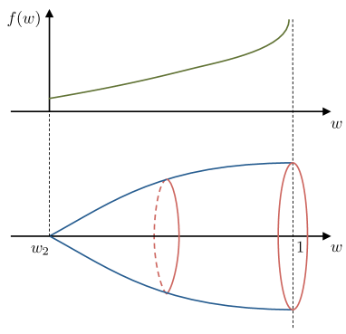
Figure 6: A schematic depiction of the internal geometry in Case II. The $z$ circle is fibered over the $w$ interval to yield $\Sigma$. In the metric $ds^{2}(\Sigma)$ in (2.1), $\Sigma$ has the topology of a disk with a $\mathbb{Z}_{\ell}$ orbifold singularity at the center. We also depict the qualitative behavior of the $AdS_{5}$ warp function $f(w)=2\,B\,w^{3/5}/\sqrt{1-w^{2}}$.

Case III.

This case is similar to Case I, except that the function $h(w)$ has a double zero at $w=1/\sqrt{2}$. As a result the $z$ circle does not shrink smoothly for any value of the constant $\mathcal{C}$. Instead, if we set $w=\tfrac{1}{\sqrt{2}}-\frac{1}{R}$, as we consider $R\rightarrow+\infty$ the 7d line element is approximately given by

$$m^{2}\,ds^{2}_{7}\approx 2^{6/5}\,ds^{2}(AdS_{5})+\frac{1}{2^{4/5}}\,\frac{dR^{2}+32\,\mathcal{C}^{2}\,dz^{2}}{R^{2}}\ ,\qquad R\rightarrow+\infty\ .$$ (A.78)

The behavior near $w=0$ is similar to Case I.

Case IV.

The behavior as we approach $w=1/\sqrt{2}$ from the right is similar to the behavior of Case III approaching $w=1/\sqrt{2}$ from the left. The behavior in the limit $w\rightarrow 1^{-}$ is as in Case II, with a decompactification of the $z$ circle.

Case V.

This case combines the features of Case I near $w=0$ and the features of Case II near $w=1$.

Case VI.

As $w\rightarrow 1^{+}$, the $z$ circle decompactifies and the $AdS_{5}$ warp factor diverges. If we set $w=1+B^{2}\,\mathcal{C}^{4}\,r^{4}/8$ and consider $r\rightarrow 0^{+}$, the line element takes the form

$$m^{2}\,ds^{2}_{7}\approx\frac{4}{r^{2}}\,\Big{[}\frac{1}{\mathcal{C}^{2}}\,ds^{2}(AdS_{5})+dr^{2}+dz^{2}\Big{]}\ ,\qquad r\rightarrow 0^{+}\ .$$ (A.79)

As we approach $w=w_{3}$, the $z$ circle shrinks. If we impose

$$|\mathcal{C}|=\frac{1}{\ell\,\sqrt{1+B^{2}}}\ ,\qquad\ell=1,2,3,\dots\ ,$$ (A.80)

we get an $\mathbb{R}^{2}/\mathbb{Z}_{\ell}$ orbifold point.

Appendix B Solutions in Canonical $\mathcal{N}=2$ Form

In this appendix we describe in greater detail the change of variables that brings the uplifted solution (2.2), (2.24) into canonical $\mathcal{N}=2$ LLM form (2.3.3). We also review some general facts about Killing spinors and spinor bilinears for LLM setups and their connections with the most general supersymmetric $AdS_{5}$ solution of 11d supergravity discussed in Gauntlett:2004zh .

B.1 Change of Variables to LLM Form

All solutions discussed in this paper fall into a subclass of the canonical LLM form (2.3.3) with an enhanced $U(1)$ isometry. In terms of the polar coordinates $(r,\beta)$ in the $(x_{1},x_{2})$ plane introduced in (2.47), the function $D$ depends on $y$ and $r$ only, and therefore the same holds true for the warp factor $\widetilde{\lambda}$, determined by $D$ via (2.44). It follows that $\partial_{\beta}$ is a Killing vector. When the function $D$ is independent of $\beta$, the Toda equation (2.45) and the expression (2.46) for the 1-form $v$ take a simpler form,

$$\bigg{(}\partial_{r}^{2}+\frac{1}{r}\,\partial_{r}\bigg{)}D+\partial_{y}^{2}e^{D}=0\ ,\qquad v=-\frac{1}{2}\,r\,\partial_{r}D\,d\beta\ .$$ (B.1)

The relation between the LLM angular variables $\chi$, $\beta$ and the angular variables $\phi$, $z$ in (2.2) was given in (2.48), repeated here for convenience as

$$\begin{pmatrix}d\chi\\ d\beta\end{pmatrix}=\begin{pmatrix}1+\mathcal{C}^{-1}&-1\\ -\mathcal{C}^{-1}&1\end{pmatrix}\,\begin{pmatrix}d\phi\\ dz\end{pmatrix}\ ,\qquad\begin{pmatrix}\partial_{\chi}\\ \partial_{\beta}\end{pmatrix}=\begin{pmatrix}1&\mathcal{C}^{-1}\\ 1&1+\mathcal{C}^{-1}\end{pmatrix}\,\begin{pmatrix}\partial_{\phi}\\ \partial_{z}\end{pmatrix}\ .$$ (B.2)

The matrix that implements this linear change of coordinates has determinant 1, consistent with the fact that all these four angular variables have period $2\pi$. As anticipated in the main text, the LLM coordinates $y$, $r$ are related to the coordinates $\mu$, $w$ in (2.2) via

$$y=\frac{4\,B\,w\,\mu}{\sqrt{\kappa\,(1-w^{2})}}\ ,\qquad r=(1-\mu^{2})^{-\frac{1}{2\mathcal{C}}}\,\mathcal{G}(w)\ ,$$ (B.3)

where the function $\mathcal{G}(w)$ is determined up to an overall constant normalization and is a solution to the ODE

$$\frac{\mathcal{G}^{\prime}(w)}{\mathcal{G}(w)}=\frac{-B\,w}{\mathcal{C}\,\left(1-w^{2}\right)\left[B-2\,w\,\sqrt{\kappa\,(1-w^{2})}\right]}\ .$$ (B.4)

For the choice of parameters and range of $w$ specified in (2.5), $\mathcal{G}(w)$ is given explicitly as

$$\mathcal{G}(w) =\mathcal{G}_{0}\,\exp\bigg{\{}-\frac{1}{2\,\mathcal{C}}\,\log(1-w^{2})+\frac{1-\mathcal{B}}{2\,\mathcal{C}\,\mathcal{B}}\,\log(1-\mathcal{B}-2\,w^{2})$$ (B.5)

$$-\frac{1+\mathcal{B}}{4\,\mathcal{C}\,\mathcal{B}}\,\log\Big{[}(\sqrt{2}-\sqrt{1-w^{2}}\,\sqrt{1-\mathcal{B}}-w\,\sqrt{1+\mathcal{B}})\,(\sqrt{2}+\sqrt{1-w^{2}}\,\sqrt{1-\mathcal{B}}+w\,\sqrt{1+\mathcal{B}})\Big{]}$$

$$-\frac{1-\mathcal{B}}{4\,\mathcal{C}\,\mathcal{B}}\,\log\Big{[}(\sqrt{2}+\sqrt{1-w^{2}}\,\sqrt{1+\mathcal{B}}-w\,\sqrt{1-\mathcal{B}})\,(\sqrt{2}-\sqrt{1-w^{2}}\,\sqrt{1+\mathcal{B}}+w\,\sqrt{1-\mathcal{B}})\Big{]}\bigg{\}}\ ,$$

where $\mathcal{G}_{0}$ is an integration constant and we have introduced the shorthand notation

$$\mathcal{B}=\sqrt{1-B^{2}}\ .$$ (B.6)

The quantity $D$, expressed in terms of $w$ and $\mu$, is given as

$$e^{D}=\frac{16\,B\,\mathcal{C}^{2}\,\left(1-\mu^{2}\right)^{1+1/\mathcal{C}}\,\left[B-2\,w\,\sqrt{\kappa\,(1-w^{2})}\right]}{\kappa\,\left(1-w^{2}\right)\,\mathcal{G}(w)^{2}}\ .$$ (B.7)

Using the chain rule, (B.7), (B.3), (B.4) one computes the derivatives of $D$ with respect to $y$ and $r$. The expressions for $\partial_{y}D$, $\partial_{r}D$, and the warp factor, computed from (2.44), are

$$-\partial_{y}D =\frac{\kappa\,(1-w^{2})\,\mu}{2\,B\,\Big{[}\mu^{2}\,h+B\,w^{2}\,(1-\mu^{2})\Big{]}}\ ,\qquad e^{-6\widetilde{\lambda}}=\frac{[\kappa\,(1-w^{2})]^{3/2}}{8\,B^{3}\,w\,\mathcal{H}}\ ,$$

$$r\,\partial_{r}D =\frac{B\,(1-\mu^{2})\,\Big{[}\mathcal{C}-2w^{2}(\mathcal{C}+1)\Big{]}-h\,(\mathcal{C}+2\mu^{2}+\mathcal{C}\mu^{2})}{\mu^{2}\,h+B\,w^{2}\,(1-\mu^{2})}$$ (B.8)

The second derivatives of $D$ are computed in a similar way and can be used to verify that $D$ satisfies the Toda equation in the form (B.1).

In order to verify that the $G_{4}$ flux (2.24) matches with the LLM expression, it is convenient to observe that the LLM $G_{4}$ flux is $G_{4}=1/(4m^{2})\,{\rm vol}_{S^{2}}\wedge\Omega_{2}$, where

$$\Omega_{2} :=D\chi\wedge d(y^{3}\,e^{-6\widetilde{\lambda}})+y\,(1-y^{2}\,e^{-6\widetilde{\lambda}})\,dv-\frac{1}{2}\,\partial_{y}e^{D}\,dx_{1}\wedge dx_{2}$$

$$=d\Big{[}-y^{3}\,e^{-6\widetilde{\lambda}}\,D\chi-y\,v\Big{]}+\frac{1}{2}\,(r\,\partial_{r}D\,dy-\partial_{y}e^{D}\,r\,dr)\wedge d\beta\ .$$ (B.9)

The 1-form $(r\,\partial_{r}D\,dy-\partial_{y}e^{D}\,r\,dr)$ is closed by virtue of the Toda equation, hence locally exact. For the solutions we are discussing, one verifies indeed that

$$r\,\partial_{r}D\,dy-\partial_{y}e^{D}\,r\,dr=d\mathcal{F}\ ,\qquad\mathcal{F}:=\frac{-8\,B\,w\,\mu\,(\mathcal{C}+1)}{\sqrt{\kappa\,(1-w^{2})}}+8\,\mathcal{C}\,\mu\ .$$ (B.10)

The above relations can be used to check that

$$\Omega_{2}=d\Big{[}-y^{3}\,e^{-6\widetilde{\lambda}}\,D\chi-y\,v+\tfrac{1}{2}\,\mathcal{F}\,d\beta\Big{]}=-4\,d\bigg{[}\frac{\mu^{3}}{\mu^{2}+w^{2}\,(1-\mu^{2})}\,D\phi\bigg{]}\ .$$ (B.11)

In the second step we have used the definition (2.46) of $D\chi$, the definition (2.23) of $D\phi$, and the change of variables (B.2). The expression (B.11) for $\Omega_{2}$ shows that the $G_{4}$ flux in (2.3.3) matches exactly with (2.24).

B.2 Killing Spinors and Calibration

In this section we review some facts about Killing spinors for the general LLM solution (2.3.3). In particular, we are interested in establishing a precise map with the Killing spinors and bilinears of the most general supersymmetric $AdS_{5}$ solution of 11d supergravity analyzed in Gauntlett-Martelli-Sparks-Waldram (GMSW) Gauntlett:2004zh . Our aim is to study calibration conditions for wrapped M2-branes in the solutions described in this work.

B.2.1 Killing Spinors and Spinor Bilinears in LLM

Killing spinors and their bilinears for LLM solutions are described in detail in the appendices of the original paper Lin:2004nb . The spinor bilinear analysis of Lin:2004nb is performed for stationary 11d solutions containing an $S^{5}$ and an $S^{2}$ factor. They are related to the $AdS_{5}$ solutions (2.3.3) by a double analytic continuation of $S^{5}$ to $AdS_{5}$ and time to the angle $\chi$. Instead of following the analytic continuation, we find it convenient to repeat the steps of Lin:2004nb directly for the $AdS_{5}$ case. Our main objective is to set a consistent set of conventions and notation, so we will be brief and refer to the original paper for further explanations of some aspects of the Killing spinor analysis.

Split of $M_{6}$ Into $S^{2}$ and $M_{4}$.

The parametrization of the 11d line element and $G_{4}$ flux is

$$ds^{2}_{11}=m^{-2}\,e^{2\widetilde{\lambda}}\,\Big{[}ds^{2}(AdS_{5})+ds^{2}(M_{6})\Big{]}\ ,\qquad G_{4}=m^{-3}\,\mathcal{G}_{4}\ ,$$ (B.12)

where $ds^{2}(AdS_{5})$ has unit radius and $\widetilde{\lambda}$ is the warp factor. This is the same parametrization as in Gauntlett:2004zh , except that we have factored out the overall scale $m^{-2}$. The quantity $\mathcal{G}_{4}$ is a closed form on $M_{6}$. As in Gauntlett:2004zh the Killing spinor of 11d supergravity is decomposed as $\psi_{\rm AdS}\otimes e^{\widetilde{\lambda}/2}\,\xi$, where $\psi_{\rm AdS}$ is a Killing spinor on $AdS_{5}$ and $\xi$ is a Dirac (non-chiral) spinor on $M_{6}$. The BPS equations for $\xi$ are derived in Gauntlett:2004zh . We write them with $m=1$ because we have factored out the overall scale. They read

$$\Big{[}\nabla_{m}+\tfrac{i}{2}\,\gamma_{m}\,\gamma_{7}-\tfrac{1}{24}\,e^{-3\widetilde{\lambda}}\,\mathcal{G}_{mn_{1}n_{2}n_{3}}\,\gamma^{n_{1}n_{2}n_{3}}\Big{]}\,\xi =0\ ,$$

$$\Big{[}\gamma^{m}\,\nabla_{m}\widetilde{\lambda}+\tfrac{1}{144}\,e^{-3\widetilde{\lambda}}\,\mathcal{G}_{n_{1}n_{2}n_{3}n_{4}}\,\gamma^{n_{1}n_{2}n_{3}n_{4}}-i\,\gamma_{7}\Big{]}\,\xi =0\ .$$ (B.13)

The indices $m,n=1,\dots,6$ are curved indices on $M_{6}$, which are raised/lowered with the metric $ds^{2}(M_{6})$ defined by (B.12). Throughout this appendix, flat indices are underlined to distinguish them from curved indices. Thus the 6d gamma matrices with flat indices are denoted $\gamma^{\underline{m}}$. They are Hermitian and obey the Clifford algebra $\{\gamma^{\underline{m}},\gamma^{\underline{n}}\}=2\,\delta^{\underline{m}\underline{n}}$. The chirality matrix $\gamma_{7}$ is defined as $\gamma_{7}=\gamma^{\underline{1}}\dots\gamma^{\underline{6}}$, is anti-Hermitian, and satisfies $\gamma_{7}^{2}=-1$. As usual, a gamma matrix with several indices denotes the product of gamma matrices totally antisymmetrized with weight 1.

To specialize the general BPS equations (B.2.1) to LLM setups, we write the internal metric $ds^{2}(M_{6})$ in the form

$$ds^{2}(M_{6})=e^{2A}\,ds^{2}(S^{2})+ds^{2}(M_{4})\ ,$$ (B.14)

where $ds^{2}(S^{2})$ is the metric on a unit-radius round sphere, $ds^{2}(M_{4})$ is a Riemannian metric on a 4d space $M_{4}$, and $A$ is a function on $M_{4}$. The $G_{4}$ flux is parametrized as

$$\mathcal{G}_{4}=F\wedge{\rm vol}_{S^{2}}\ ,$$ (B.15)

where ${\rm vol}_{S^{2}}$ is the volume form of the metric $ds^{2}(S^{2})$ and $F$ is a closed 2-form on $M_{4}$. The 6d index $m$ is split as $m=(x,\alpha)$, with $x=1,2$ for the $S^{2}$ directions and $\alpha=1,2,3,4$ for the $M_{4}$ directions. Following Lin:2004nb , we split the 6d gamma matrices $\gamma^{m}$ as

$$\gamma^{\underline{x}}=\sigma^{\underline{x}}\otimes\Gamma_{5}\ ,\qquad\gamma^{\underline{\alpha}}=1\otimes\Gamma^{\underline{\alpha}}\ ,$$ (B.16)

where $\sigma^{\underline{x}=1,2}$ are the standard Pauli matrices and the 4d gamma matrices $\Gamma^{\underline{\alpha}}$ are Hermitian and satisfy $\{\Gamma^{\underline{\alpha}},\Gamma^{\underline{\beta}}\}=2\,\delta^{\underline{\alpha}\underline{\beta}}$. The 4d chirality matrix $\Gamma_{5}$ is defined as $\Gamma_{5}=\Gamma^{\underline{1}}\dots\Gamma^{\underline{4}}$, is Hermitian, and satisfies $\Gamma_{5}^{2}=1$.

We decompose the 6d Dirac spinor $\xi$ that enters the BPS conditions (B.2.1) into Killing spinors on $S^{2}$ and Dirac spinors on $M_{4}$. More precisely, we write

$$\xi^{\mathcal{I}}=\vartheta^{\mathcal{I}}\otimes\epsilon_{+}+(i\,\sigma^{3}\,\vartheta^{\mathcal{I}})\otimes\epsilon_{-}\ .$$ (B.17)

In the above relation, $\epsilon_{\pm}$ are Dirac spinors on $M_{4}$ while $\vartheta^{\mathcal{I}}$ is a basis of independent Killing 2-component spinors on $S^{2}$, satisfying

$$\nabla_{x}^{S^{2}}\vartheta^{\mathcal{I}}=+\frac{i}{2}\,\sigma_{x}\,\vartheta^{\mathcal{I}}\ .$$ (B.18)

The index $\mathcal{I}=1,2$ is not a spinor index, but rather labels the two linearly independent solutions to the above equation. We can regard $\mathcal{I}$ as a fundamental index of the isometry algebra $\mathfrak{su}(2)\cong\mathfrak{so}(3)$ of the round $S^{2}$. The fact that the 6d spinor $\xi$ carries a label $\mathcal{I}=1,2$ is simply the statement that we are seeking solutions preserving 4d $\mathcal{N}=2$ superconformal symmetry. Notice that the spinor $(i\,\sigma^{3}\,\vartheta^{\mathcal{I}})$ satisfies the Killing equation (B.18) with $+i$ on the RHS replaced with $-i$.

The spinors $\epsilon_{\pm}$ are not independent, but rather related as (see Lin:2004nb and also OColgain:2010ev )

$$\epsilon_{-}=-a\,\Gamma_{5}\,\epsilon_{+}\ ,\qquad a=\pm 1\ .$$ (B.19)

As a result, we can also write the expression (B.17) for $\xi$ as

$$\xi^{\mathcal{I}}=(1-a\,\gamma_{7})\,(\vartheta^{\mathcal{I}}\otimes\epsilon)\ ,\qquad\epsilon\equiv\epsilon_{+}\ .$$ (B.20)

The BPS equations (B.2.1) imply the following conditions on $\epsilon$,

$$\nabla_{\alpha}\widetilde{\lambda}\,\Gamma^{\alpha}\,\epsilon+\tfrac{a}{12}\,e^{-3\widetilde{\lambda}-2A}\,F_{\alpha\beta}\,\Gamma^{\alpha\beta}\,\Gamma_{5}\,\epsilon-i\,a\,\epsilon =0\ ,$$

$$\nabla_{\alpha}\epsilon+\tfrac{i\,a}{2}\,\Gamma_{\alpha}\,\epsilon-\tfrac{a}{4}\,e^{-3\widetilde{\lambda}-2A}\,F_{\alpha\beta}\,\Gamma^{\beta}\,\Gamma_{5}\,\epsilon =0\ ,$$

$$\nabla_{\alpha}A\,\Gamma^{\alpha}\,\epsilon+i\,e^{-A}\,\Gamma_{5}\,\epsilon+i\,a\,\epsilon-\tfrac{a}{4}\,e^{-3\widetilde{\lambda}-2A}\,F_{\alpha\beta}\,\Gamma^{\alpha\beta}\,\Gamma_{5}\,\epsilon =0\ .$$ (B.21)

Dirac Bilinears.

We are now in a position to retrace the steps of Lin:2004nb to study bilinears constructed with $\epsilon$ and projection conditions on $\epsilon$. Dirac bilinears are constructed with $\bar{\epsilon}\equiv\epsilon^{\dagger}$. The scalar bilinear is a constant: we choose the normalization

$$\bar{\epsilon}\,\epsilon=1\ .$$ (B.22)

The pseudo-scalar bilinear defines a non-trivial 0-form on $M_{4}$. The Fierz rearrangements

$$(\bar{\epsilon}\,\Gamma^{\alpha}\,\epsilon)^{2}=-(\bar{\epsilon}\,\Gamma^{\alpha}\,\Gamma_{5}\epsilon)^{2}=(\bar{\epsilon}\,\epsilon)^{2}-(\bar{\epsilon}\,\Gamma_{5}\,\epsilon)^{2}\ ,$$ (B.23)

together with the fact that $\bar{\epsilon}\,\Gamma^{\alpha}\,\epsilon$ is real and $\bar{\epsilon}\,\Gamma^{\alpha}\,\Gamma_{5}\epsilon$ purely imaginary, show that $|\bar{\epsilon}\,\Gamma_{5}\,\epsilon|\leq|\bar{\epsilon}\,\epsilon|=1$. Therefore, we can parametrize $\bar{\epsilon}\,\Gamma_{5}\,\epsilon$ as

$$\bar{\epsilon}\,\Gamma_{5}\,\epsilon=-\sin\zeta\ ,$$ (B.24)

with $\zeta\in[-\pi/2,\pi/2]$. The quantity $\zeta$ is related to the canonical coordinate $y$ in LLM form (2.3.3) via

$$y=e^{3\widetilde{\lambda}}\,\sin\zeta\ .$$ (B.25)

The vector bilinear defines a Killing vector, which is identified with the canonical angular direction $\chi$ in the standard LLM form (2.3.3). More precisely, if $y^{\alpha}$ are local coordinates on $M_{4}$, we can write

$$\bar{\epsilon}\,\Gamma^{\alpha}\,\epsilon\,\frac{\partial}{\partial y^{\alpha}}=\frac{\partial}{\partial\chi}\ .$$ (B.26)

The pseudo-vector bilinear $\bar{\epsilon}\,\Gamma_{\alpha}\,\Gamma_{5}\,\epsilon$ turns out to be given in terms of the warp factor and the derivative of the pseudo-scalar bilinear $\bar{\epsilon}\,\Gamma_{5}\,\epsilon$. More precisely, we can write

$$\bar{\epsilon}\,\Gamma_{\alpha}\,\Gamma_{5}\,\epsilon\,dy^{\alpha}=-\frac{i\,a}{2}\,e^{-3\widetilde{\lambda}}\,dy\ .$$ (B.27)

The Fierz rearrangements (B.23), together with the additional Fierz identity

$$(\bar{\epsilon}\Gamma^{\alpha}\epsilon)(\bar{\epsilon}\Gamma_{\alpha}\Gamma_{5}\epsilon)=0\ ,$$ (B.28)

can also be used to constrain the form of the metric on $M_{4}$. Together with the coordinates $\chi$, $y$ defined in (B.26), (B.25), we have two coordinates $x^{i}$, $i=1,2$. The line element reads

$$ds^{2}(M_{4})=\cos^{2}\zeta\,(d\chi+v_{i}\,dx^{i})^{2}+\frac{1}{4\,e^{6\widetilde{\lambda}}\,\cos^{2}\zeta}\,(dy^{2}+\gamma_{ij}\,dx^{i}\,dx^{j})\ .$$ (B.29)

Notice how (B.28) is exploited by choosing the coordinate $y$ not to have any mixed metric component with any other coordinate. The quantities $\zeta$, $v_{i}$, $\gamma_{ij}$ and the warp factor depend on $y$, $x^{i}$, but not on $\chi$. A natural vielbein for $ds^{2}(M_{4})$ is

$$e^{\underline{\chi}}=\cos\zeta\,D\chi\equiv\cos\zeta\,(d\chi+v_{i}\,dx^{i})\ ,\qquad e^{\underline{y}}=\frac{1}{2\,e^{3\widetilde{\lambda}}\,\cos\zeta}\ ,\qquad e^{\underline{i}}=\frac{1}{2\,e^{3\widetilde{\lambda}}\,\cos\zeta}\,\widehat{e}^{\underline{i}}\ ,$$ (B.30)

where $\widehat{e}^{\underline{1}}$, $\widehat{e}^{\underline{2}}$ is a vielbein for $\gamma_{ij}$. We choose the orientation $i=1$, $i=2$, $\chi$, $y$, so that $\epsilon_{\underline{1}\underline{2}\underline{\chi}\underline{y}}=1$ and $\Gamma_{5}=\Gamma_{\underline{1}}\,\Gamma_{\underline{2}}\,\Gamma_{\underline{\chi}}\,\Gamma_{\underline{y}}$.

Following the steps detailed in appendix F.2 of Lin:2004nb , one can manipulate the BPS conditions (B.2.1) on $\epsilon$ to determine the function $A$ and the 2-form $F$. The function $A$ is

$$e^{A}=-\frac{a}{2}\,\sin\zeta\ .$$ (B.31)

The coordinate $y$ in LLM form is non-negative. Comparing (B.25) and (B.31) we see that we have to choose the sign $a$ to be

$$a=-1\ .$$ (B.32)

The sign of $a$ is correlated to our choice (B.24). We could perform the redefinition $\zeta\rightarrow-\zeta$ and change the sign of $a$. The 2-form $F$ is given by

$$F =\frac{3}{4}\,\frac{y^{2}\,e^{-6\widetilde{\lambda}}}{1-y^{2}\,e^{-6\widetilde{\lambda}}}\,*_{3}d\widetilde{\lambda}+\frac{1}{4}\,D\chi\wedge d(y^{3}\,e^{-6\widetilde{\lambda}})\ ,$$ (B.33)

where $*_{3}$ denotes the Hodge star operation associated to the line element $dy^{2}+\gamma_{ij}\,dx^{i}\,dx^{j}$, with ordering $i=1$, $i=2$, $y$.

Projection Conditions.

We may now plug the values of $A$ and $F$ in the first and third BPS equation in (B.2.1). The resulting algebraic conditions on the spinor $\epsilon$ can be manipulated to take the form of projection conditions. More precisely, one finds

$$\Big{[}1-i\,\Gamma^{\underline{1}\underline{2}}\Big{]}\epsilon=0\ ,\qquad\Big{[}\cos\zeta+i\,\sin\zeta\,\Gamma^{\underline{y}}+i\,\Gamma^{\underline{y}}\,\Gamma_{5}\Big{]}\epsilon=0\ .$$ (B.34)

These relations take a simpler form in terms of the rescaled spinor

$$\widetilde{\epsilon}=e^{\frac{i}{2}\,\zeta\,\Gamma^{\underline{y}}}\,\epsilon\ ,$$ (B.35)

since they can be written as

$$\Big{[}1-i\,\Gamma^{\underline{1}\underline{2}}\Big{]}\widetilde{\epsilon}=0\ ,\qquad\Big{[}1+i\,\Gamma^{\underline{y}}\,\Gamma_{5}\Big{]}\widetilde{\epsilon}=0\ .$$ (B.36)

These relations demonstrate that $\widetilde{\epsilon}$ has only one independent component. Moreover we can always use a local Lorentz rotation to make sure that $\widetilde{\epsilon}$ is independent of the coordinates $y$, $x^{1}$, $x^{2}$. (Its $\chi$ dependence will be fixed momentarily.)

Majorana Bilinears.

To proceed we follow Lin:2004nb and construct a Majorana 1-form bilinear. The 4d charge conjugation matrix $C$ satisfies

$$(\Gamma^{\alpha})^{T}=-C\,\Gamma^{\alpha}\,C^{-1}\ ,\qquad C^{T}=-C\ .$$ (B.37)

The bilinear of interest is

$$\omega_{1}=\epsilon^{T}\,C\,\Gamma_{\alpha}\,\epsilon\,dy^{\alpha}\ .$$ (B.38)

Since the matrices $C$, $C\,\Gamma_{5}$, and $C\,\Gamma^{\alpha}\,\Gamma_{5}$ are antisymmetric, and the spinor $\epsilon$ is Grassmann even, the bilinears $\epsilon^{T}\,C\,\epsilon$, $\epsilon^{T}\,C\,\Gamma_{5}\,\epsilon$, and $\epsilon^{T}\,C\,\Gamma^{\alpha}\,\Gamma_{5}\,\epsilon$ are all identically zero. This information, combined with the projection conditions (B.34), allow one to conclude that the 1-form $\omega_{1}$ has only one independent component, because

$$\epsilon^{T}\,C\,\Gamma^{\underline{y}}\,\epsilon=0\ ,\qquad\epsilon^{T}\,C\,\Gamma^{\underline{\chi}}\,\epsilon=0\ ,\qquad\epsilon^{T}\,C\,\Gamma^{\underline{2}}\,\epsilon=-i\,\epsilon^{T}\,C\,\Gamma^{\underline{1}}\,\epsilon\ .$$ (B.39)

The definition (B.35) implies

$$\epsilon^{T}\,C\,\Gamma^{\underline{1}}\,\epsilon=\cos\zeta\,\widetilde{\epsilon}^{T}\,C\,\Gamma^{\underline{1}}\,\widetilde{\epsilon}\ .$$ (B.40)

Using this relation, the 1-form $\omega_{1}$ can be cast in the form

$$\omega_{1}=\frac{1}{2}\,e^{-3\widetilde{\lambda}}\,(\widetilde{\epsilon}^{T}\,C\,\Gamma^{\underline{1}}\,\widetilde{\epsilon})\,\big{(}\widehat{e}^{\underline{1}}-i\,\widehat{e}^{\underline{2}}\big{)}\ ,$$ (B.41)

where $\widehat{e}^{\underline{1}}$, $\widehat{e}^{\underline{2}}$ is a vielbein for the $\gamma_{ij}$ metric in (B.29). The 2-form $d\omega_{1}$ can be computed making use of the BPS equations (B.2.1), with the result

$$d\omega_{1}=\frac{i}{4}\,(\epsilon^{T}\,C\,\Gamma_{\alpha\beta}\,\epsilon)\,dy^{\alpha}\wedge dy^{\beta}-3\,d\widetilde{\lambda}\wedge\omega_{1}\ .$$ (B.42)

The components of the bilinear $\epsilon^{T}\,C\,\Gamma_{\alpha\beta}\,\epsilon$ are greatly constrained by the projection conditions (B.34). Combining them with the fact that $\epsilon^{T}\,C\,\Gamma^{\alpha}\,\Gamma_{5}\,\epsilon$ is identically zero, one verifies

$$i\,\epsilon^{T}\,C\,\Gamma_{\underline{y}\underline{2}}\,\epsilon=\epsilon^{T}\,C\,\Gamma_{\underline{y}\underline{1}}\,\epsilon=i\,\tan\zeta\,\epsilon^{T}\,C\,\Gamma_{\underline{1}}\,\epsilon\ ,\qquad i\,\epsilon^{T}\,C\,\Gamma_{\underline{\chi}\underline{2}}\,\epsilon=\epsilon^{T}\,C\,\Gamma_{\underline{y}\underline{1}}\,\epsilon=-\frac{1}{\cos\zeta}\,\epsilon^{T}\,C\,\Gamma_{\underline{1}}\,\epsilon\ ,$$

$$\epsilon^{T}\,C\,\Gamma_{\underline{1}\underline{2}}\,\epsilon=0=\epsilon^{T}\,C\,\Gamma_{\underline{\chi}\underline{y}}\,\epsilon\ .$$ (B.43)

These relations allow one to recast the equation for $d\omega_{1}$ in the form

$$d\omega_{1}=\bigg{[}-\frac{y\,e^{-6\widetilde{\lambda}}}{2\,(1-y^{2}\,e^{-6\widetilde{\lambda}})}\,dy-i\,D\chi-3\,d\widetilde{\lambda}\bigg{]}\wedge\omega_{1}\ .$$ (B.44)

As explained in Lin:2004nb , using (B.41) and the fact that the rescaled spinor $\widetilde{\epsilon}$ is independent of $y$, $x^{1}$, $x^{2}$, one can use (B.44) to argue that the vielbein for the metric $\gamma_{ij}$ can be chosen to be

$$\widehat{e}^{1}=e^{D/2}\,dx^{1}\ ,\qquad\widehat{e}^{2}=e^{D/2}\,dx^{2}\ ,$$ (B.45)

for some function $D$ of $y$, $x^{1}$, $x^{2}$ (which is ultimately identified with the function $D$ in the canonical LLM form). Once this choice for $\widehat{e}^{1}$, $\widehat{e}^{2}$ is made, the various components of the equation (B.44) can be studied separately and yield the following results. Firstly, the warp factor is determined by the function $D$ by the expression (2.44). Secondly, the $\chi$ dependence of the rescaled spinor $\widetilde{\epsilon}$ is determined to be

$$\partial_{\chi}\,\widetilde{\epsilon}=-\frac{i}{2}\,\widetilde{\epsilon}\ .$$ (B.46)

Finally, the quantities $v_{i}$ in the metric (B.29) are fixed in terms of the function $D$ as

$$v_{1}=+\frac{1}{2}\,\partial_{2}D\ ,\qquad v_{2}=-\frac{1}{2}\,\partial_{1}D\ .$$ (B.47)

Toda Equation and Final Form of the 2-form $F$.

The relation (B.26) and the form of the metric (B.29) imply that

$$\alpha_{1}:=(\bar{\epsilon}\,\Gamma_{\alpha}\,\epsilon)\,dy^{\alpha}=\cos^{2}\zeta\,D\chi=(1-y^{2}\,e^{-6\widetilde{\lambda}})\,D\chi\ .$$ (B.48)

On the one hand, the 2-form $d\alpha_{1}$ is readily computed from this expression for $\alpha_{1}$. On the other hand, the BPS equations (B.2.1) imply the following equation for $d\alpha_{1}$,

$$d\alpha_{1}=-2\,i\cdot\tfrac{1}{2}\,(\bar{\epsilon}\,\Gamma_{\alpha\beta}\,\epsilon)\,dy^{\alpha}\wedge dy^{\beta}-e^{-3\widetilde{\lambda}-2A}\,(\bar{\epsilon}\,\Gamma_{5}\,\epsilon)\,F\ .$$ (B.49)

The components of $\bar{\epsilon}\,\Gamma_{\alpha\beta}\,\epsilon$ are constrained by the projection conditions (B.34). For example, we have $\Gamma^{\underline{2}}\,\epsilon=-i\,\Gamma^{\underline{1}}\,\epsilon$ and $\bar{\epsilon}\,\Gamma^{\underline{1}}=-i\,\bar{\epsilon}\,\Gamma^{\underline{2}}$, and therefore

$$\bar{\epsilon}\,\Gamma^{\underline{y}}\,\Gamma^{\underline{1}}\,\epsilon=-(\bar{\epsilon}\,\Gamma^{\underline{1}})\,\Gamma^{\underline{y}}\,\epsilon=i\,\bar{\epsilon}\,\Gamma^{\underline{2}}\,\Gamma^{\underline{y}}\,\epsilon=-i\,\bar{\epsilon}\,\Gamma^{\underline{y}}\,(\Gamma^{\underline{2}}\,\epsilon)-\bar{\epsilon}\,\Gamma^{\underline{y}}\,\Gamma^{\underline{1}}\,\epsilon\ ,$$ (B.50)

which shows that $\bar{\epsilon}\,\Gamma^{\underline{y}}\,\Gamma^{\underline{1}}\,\epsilon=0$. By similar arguments, one verifies that the only independent non-zero components of $\bar{\epsilon}\,\Gamma_{\alpha\beta}\,\epsilon$ are

$$\bar{\epsilon}\,\Gamma_{\underline{1}\underline{2}}\,\epsilon=-i\ ,\qquad\bar{\epsilon}\,\Gamma_{\underline{\chi}\underline{y}}\,\epsilon=-i\,\sin\zeta\ .$$ (B.51)

This information, combined with the expressions (B.31), (B.33) for $A$ and $F$, allows us to make a direct comparison between the relation (B.49) for $d\alpha_{1}$ and the actual value of $d\alpha_{1}$ as computed from (B.48). The $dx^{1}\wedge dx^{2}$ piece of the resulting 2-form equation, using (B.47), implies the Toda equation for $D$ (2.45).

Having established that $D$ satisfies the Toda equation, we can revisit the expression (B.33) for $F$ and make use of the identity

$$3\,\frac{y^{2}\,e^{-6\lambda}}{1-y^{2}\,e^{-6\lambda}}\,*_{3}d\widetilde{\lambda} =y\,(1-y^{2}\,e^{-6\lambda})\,dv-\frac{1}{2}\,\partial_{y}e^{D}\,dx^{1}\wedge dx^{2}$$

$$+\frac{y}{2\,(1-y\,\partial_{y}D)}\,(\partial_{1}^{2}D+\partial_{2}^{2}D+\partial_{y}^{2}e^{D})\ .$$ (B.52)

Since the term on the second line is zero, we can rewrite $F$ as

$$F=\frac{1}{4}\,\bigg{[}y\,(1-y^{2}\,e^{-6\lambda})\,dv-\frac{1}{2}\,\partial_{y}e^{D}\,dx^{1}\wedge dx^{2}+D\chi\wedge d(y^{3}\,e^{-6\widetilde{\lambda}})\bigg{]}\ ,$$ (B.53)

Using (B.12) and (B.15), this expression for $F$ implies that $G_{4}$ is given by the expression quoted in (2.3.3).

B.2.2 The Calibration 2-form $Y^{\prime}$

The calibration 2-form for supersymmetric M2-branes was identified in Gauntlett:2006ai for the most general $AdS_{5}$ solution preserving 4d $\mathcal{N}=1$ superconformal symmetry, as classified by Gauntlett, Martelli, Sparks, and Waldram (GMSW) Gauntlett:2004zh . In order to apply the results of Gauntlett:2006ai to a solution preserving 4d $\mathcal{N}=2$ superconformal symmetry, we select a linear combination $\xi$ of the two LLM spinors $\xi^{\mathcal{I}}$ in (B.20), and we identify $\xi$ with the Killing spinor of the general GMSW solution,

$$\xi=c_{\mathcal{I}}\,\xi^{\mathcal{I}}=(1+\gamma_{7})\,(c_{\mathcal{I}}\,\vartheta^{\mathcal{I}}\otimes\epsilon)\ ,$$ (B.54)

where we have used $a=-1$ and $c_{\mathcal{I}}$ are complex constants. Before proceeding, it is useful to collect some identities about bilinears of the $S^{2}$ Killing spinors $\vartheta^{\mathcal{I}}$. We set $\bar{\vartheta}_{\mathcal{I}}=(\vartheta^{\mathcal{I}})^{\dagger}$. A basis $\vartheta^{\mathcal{I}}$ of solutions to (B.18) can always be chosen, in such a way that

$$\bar{\vartheta}_{\mathcal{I}}\,\vartheta^{\mathcal{J}} =\delta^{\mathcal{J}}_{\mathcal{I}}\ , \bar{\vartheta}_{\mathcal{I}}\,\sigma^{3}\,\vartheta^{\mathcal{J}} =\hat{y}^{A}\,(\sigma_{A})^{\mathcal{J}}{}_{\mathcal{I}}\ ,$$

$$\bar{\vartheta}_{\mathcal{I}}\,\sigma_{x}\,\vartheta^{\mathcal{J}} =-\mathcal{K}_{x}{}^{A}\,(\sigma_{A})^{\mathcal{J}}{}_{\mathcal{I}}\ , \bar{\vartheta}_{\mathcal{I}}\,\sigma_{x}\,\sigma^{3}\,\vartheta^{\mathcal{J}} =i\,\partial_{x}\hat{y}^{A}\,(\sigma_{A})^{\mathcal{J}}{}_{\mathcal{I}}\ .$$ (B.55)

In the previous relations $x=1,2$ is a curved index on $S^{2}$. The Pauli matrices on the LHSs play the role of gamma matrices on $S^{2}$. The Pauli matrices on the RHSs are invariant tensors of the $\mathfrak{su}(2)\cong\mathfrak{so}(3)$ isometry algebra of $S^{2}$, connecting the indices $\mathcal{I},\mathcal{J}=1,2$ in the fundamental representation of $\mathfrak{su}(2)$ to the indices $A=1,2,3$ in the vector representation of $\mathfrak{so}(3)$. The three quantities $\hat{y}^{A}$ are real scalars in $S^{2}$, identified with the Cartesian coordinates of $\mathbb{R}^{3}$ in the standard embedding $S^{2}\subset\mathbb{R}^{3}$. The metric on $S^{2}$ is given in terms of $\hat{y}^{A}$ by

$$g_{xy}=\partial_{x}\hat{y}^{A}\,\partial_{y}\hat{y}_{A}\ .$$ (B.56)

(The $A$ indices in are raised/lowered with $\delta$.) The 1-forms $\mathcal{K}_{x}{}^{A}$ are defined as

$$\mathcal{K}_{x}{}^{A}=\epsilon^{ABC}\,\hat{y}_{B}\,\partial_{x}\hat{y}_{C}\ ,$$ (B.57)

and yield the standard Killing vectors on $S^{2}$ after raising their curved index $x$ with the $S^{2}$ metric. The 1-forms $\mathcal{K}_{x}{}^{A}$ can also be written as Hodge duals of the gradients of $\hat{y}^{A}$, because $\epsilon_{xy}\,\mathcal{K}^{xA}=\partial_{x}\hat{y}^{A}$, where $\epsilon_{12}=\sqrt{{\rm det}g_{xy}}$.

In order to preserve the normalization condition $\overline{\xi}\,\xi=2$ of Gauntlett:2004zh , the constants $c_{\mathcal{I}}$ and their complex conjugates $\bar{c}^{\mathcal{I}}$ should satisfy $c_{\mathcal{I}}\,\bar{c}^{\mathcal{I}}=1$. A choice of $c_{\mathcal{I}}$ determines a vector $n^{A}$ in $\mathbb{R}^{3}$ via the formula

$$n^{A}=c_{\mathcal{J}}\,(\sigma^{A})^{\mathcal{J}}{}_{\mathcal{I}}\,\bar{c}^{\mathcal{I}}\ .$$ (B.58)

Without loss of generality, we can select $c_{\mathcal{I}}=(1,0)$ in such a way that the 3-vector $n^{A}$ points in the direction $A=3$. (Any other choice is related by the action of the isometry group of $S^{2}$.) With this choice we have

$$\hat{y}^{A}\,n_{A}=\hat{y}^{A=3}\equiv\tau\ .$$ (B.59)

The quantity $\tau$ lies in $[-1,1]$. The other two real scalars $\hat{y}^{A=1}$, $\hat{y}^{A=2}$ are parametrized as

$$\hat{y}^{A=1}=\sqrt{1-\tau^{2}}\,\cos\varphi\ ,\qquad\hat{y}^{A=2}=\sqrt{1-\tau^{2}}\,\sin\varphi\ ,$$ (B.60)

where $\varphi$ is an angle of periodicity $2\pi$. The metric on $S^{2}$ is written in terms of $\tau$ and $\varphi$ in (2.59).

We are now in a position to discuss the calibration 2-form. It is given as

$$Y^{\prime}=\frac{1}{2}\,Y^{\prime}_{mn}\,dy^{m}\wedge dy^{n}\ ,\qquad Y^{\prime}_{mn}=\frac{1}{2}\,\bar{\xi}\,\gamma_{mn}\,\gamma_{7}\,\xi\ .$$ (B.61)

Making use of (B.54) this 2-form can be written in LLM setups as

$$Y^{\prime}_{mn} =(\bar{c}^{\mathcal{J}}\,\bar{\vartheta}_{\mathcal{J}}\otimes\bar{\epsilon})\,\gamma_{mn}\,\gamma_{7}\,(c_{\mathcal{I}}\,\vartheta^{\mathcal{I}}\otimes\bar{\epsilon})\ .$$ (B.62)

Using (B.14), (B.16), (B.2.2), we can write the 2-form $Y^{\prime}$ as

$$Y^{\prime} =-e^{2A}\,(\bar{c}^{\mathcal{I}}\,c_{\mathcal{I}})\,(\bar{\epsilon}\,\Gamma_{5}\,\epsilon)\,{\rm vol}_{S^{2}}+e^{A}\,d(\hat{y}^{A}\,n_{A})\wedge(\bar{\epsilon}\,\Gamma_{\alpha}\,\epsilon)\,dy^{\alpha}$$

$$+\frac{i}{2}\,(\hat{y}^{A}\,n_{A})\,(\bar{\epsilon}\,\Gamma_{\alpha\beta}\,\Gamma_{5}\,\epsilon)\,dy^{\alpha}\wedge dy^{\beta}\ .$$ (B.63)

To treat the last term, it is convenient to use the identity

$$\Gamma_{\alpha\beta}\,\Gamma_{5}=-\frac{1}{2}\,\epsilon_{\alpha\beta\gamma\delta}\,\Gamma^{\gamma\delta}\ .$$ (B.64)

We have already established the non-zero independent components of the bilinear $\bar{\epsilon}\,\Gamma_{\alpha\beta}\,\epsilon$. Combining our previous results, and specializing to our choice of $c_{\mathcal{I}}$ such that $\hat{y}^{A}\,n_{A}=\tau$, we obtain

$$Y^{\prime} =\frac{1}{4}\,y^{3}\,e^{-9\lambda}\,{\rm vol}_{S^{2}}+\frac{1}{2}\,y\,e^{-3\lambda}\,(1-y^{2}\,e^{-6\lambda})\,d\tau\wedge D\chi$$

$$-\frac{1}{2}\,\tau\,e^{-3\lambda}\,D\chi\wedge dy-\frac{1}{4}\,\frac{y\,e^{-9\lambda}\,\tau\,e^{D}}{1-y^{2}\,e^{-6\lambda}}\,dx^{1}\wedge dx^{2}\ .$$ (B.65)

We can also write $Y^{\prime}$ in terms of $d\phi$ and the 1-form $Dz$ defined in (2.25),

$$Y^{\prime} =\frac{\mu^{3}\,w^{3/2}\,[\kappa(1-w^{2})]^{3/4}}{\sqrt{2}\,B^{3/2}\,\mathcal{H}^{3/2}}\,{\rm vol}_{S^{2}}+\frac{\mathcal{C}\,\kappa\,\mu\,[\kappa\,(1-w^{2})]^{-3/4}}{\sqrt{2}\,\sqrt{B}\,\sqrt{w}\,\sqrt{\mathcal{H}}}\,\tau\,dw\wedge Dz$$

$$-\frac{\kappa\,\mu\,(1-\mu^{2})\,(2w^{2}-1)\,[\kappa(1-w^{2})]^{-1/4}}{\sqrt{2}\,\sqrt{B}\,\sqrt{w}\,\sqrt{\mathcal{H}}\,\Big{[}2\,B\,w\,\mathcal{H}-(\mu^{2}-1+4w^{2})\,\sqrt{\kappa(1-w^{2})}\Big{]}}\,\tau\,dw\wedge d\phi$$

$$+\frac{\mathcal{C}\,[\kappa(1-w^{2})]^{-1/4}\,\Big{[}B\,w-\sqrt{\kappa(1-w^{2})}\Big{]}}{\sqrt{2}\,B^{3/2}\,\sqrt{w}\,\sqrt{\mathcal{H}}}\,\tau\,d\mu\wedge Dz$$

$$+\frac{\mathcal{C}\,\mu\,\sqrt{w}\,[\kappa(1-w^{2})]^{1/4}\,\Big{[}B\,\mathcal{H}-w\,(1+\mu^{2})\,\sqrt{\kappa(1-w^{2})}\Big{]}}{\sqrt{2}\,B^{3/2}\,\mathcal{H}^{3/2}}\,d\tau\wedge Dz$$

$$+\frac{\sqrt{w}\,(1+\mu^{2})\,h\,[\kappa(1-w^{2})]^{3/4}}{\sqrt{2}\,B^{3/2}\,\sqrt{\mathcal{H}}\,\Big{[}2\,B\,w\,\mathcal{H}-(\mu^{2}-1+4w^{2})\,\sqrt{\kappa(1-w^{2})}\Big{]}}\,\tau\,d\mu\wedge d\phi$$

$$+\frac{\sqrt{w}\,\mu\,(1-\mu^{2})\,h\,[\kappa(1-w^{2})]^{3/4}}{\sqrt{2}\,B^{3/2}\,\sqrt{\mathcal{H}}\,\Big{[}2\,B\,w\,\mathcal{H}-(\mu^{2}-1+4w^{2})\,\sqrt{\kappa(1-w^{2})}\Big{]}}\,d\tau\wedge d\phi\ .$$ (B.66)

B.2.3 R-symmetry Charges of Wrapped M2-branes

The R-symmetry charges of wrapped M2-brane operators can be extracted using the Wess-Zumino coupling of M2-branes to $C_{3}$, as in Gauntlett:2006ai . To this end, we need to introduce external background gauge fields in $G_{4}$. This is accomplished in the construction of $E_{4}$ in section LABEL:sdsd. The final result is repeated here for convenience,

$$\!\!\!\!E_{4}=N\,e_{2}\wedge\bigg{[}d\alpha_{0\chi}\wedge\frac{(d\chi)^{\rm g}}{2\pi}+d\alpha_{0\beta}\wedge\frac{(d\beta)^{\rm g}}{2\pi}\bigg{]}+N\,\alpha_{0\chi}\,e_{2}\wedge\frac{F^{\chi}}{2\pi}-\mathcal{C}^{-1}\,\frac{f_{1}}{2\pi}\wedge e_{2}\wedge d\alpha_{0\beta}\ .\!\!\!$$ (B.67)

The 0-forms $\alpha_{0\chi}$, $\alpha_{0\beta}$ are defined in (3.4). If all external gauge fields are turned off, $E_{4}$ reduces to $\overline{G}_{4}$, which is related to the background $G_{4}$ by the relation (2.34). As a result, we can write

$$G_{4}^{\rm tot}=-(2\pi\ell_{p})^{3}\,E_{4}\ ,$$ (B.68)

where $G_{4}^{\rm tot}$ denotes the background $G_{4}$-flux dressed with external background gauge fields, written in the same normalization used in the main text in giving the solution, cfr. (2.24). To proceed, let us write

$$G_{4}^{\rm tot}=G_{4}+d\delta C_{3}\ ,$$ (B.69)

where $\delta C_{3}$ collects all terms that contain external gauge fields. For the computation at hand, we only need to retain terms linear in the external gauge fields inside $\delta C_{3}$. In the conventions we are adopting, the coupling of an M2-brane to $C_{3}$ fluctuations is given by

$$S_{\rm M2}\supset T_{\rm M2}\,\int_{\mathcal{W}_{3}}\delta C_{3}\ ,\qquad T_{\rm M2}=\frac{2\pi}{(2\pi\ell_{p})^{3}}\ ,$$ (B.70)

where $\mathcal{W}_{3}$ denotes the worldvolume of the M2-brane.

The expression of $d\delta C_{3}$ is extracted from $E_{4}-\overline{G}_{4}$. A useful identity for the $SO(3)$ global angular form $e_{2}$ is

$$e_{2}=\frac{\rm{vol}_{S^{2}}}{4\pi}-\frac{d(\hat{y}^{A}\,A_{A})}{4\pi}\ ,\qquad A=1,2,3\ ,$$ (B.71)

in conventions in which $D\hat{y}^{A}=d\hat{y}^{A}-A^{AB}\,\hat{y}_{B}=d\hat{y}^{A}-\epsilon^{ABC}\,A_{C}\,\hat{y}_{B}$. Making use of the expression (3.17) for $f_{1}$, we find the following result for $d\delta C_{3}$,

$$-\frac{d\delta C_{3}}{(2\pi\ell_{p})^{3}} =-\frac{d(\hat{y}^{a}\,A_{a})}{4\pi}\,N\,\bigg{[}d\alpha_{0\chi}\,\frac{d\chi}{2\pi}+d\alpha_{0\beta}\,\frac{d\beta}{2\pi}\bigg{]}+N\,\frac{{\rm vol}_{S^{2}}}{4\pi}\,\bigg{[}d\alpha_{0\chi}\,\frac{A^{\chi}}{2\pi}+d\alpha_{0\beta}\,\frac{A^{\beta}}{2\pi}\bigg{]}$$

$$+N\,\frac{{\rm vol}_{S^{2}}}{4\pi}\,\alpha_{0\chi}\,\frac{dA^{\chi}}{2\pi}-\mathcal{C}^{-1}\,\frac{da_{0}-N\,\mathcal{C}\,A^{\beta}}{2\pi}\,\frac{{\rm vol}_{S^{2}}}{4\pi}\,d\alpha_{0\beta}\ .$$ (B.72)

An antiderivative of the above quantity is readily extracted,

$$-\frac{\delta C_{3}}{(2\pi\ell_{p})^{3}} =-\frac{\hat{y}^{a}\,A_{a}}{4\pi}\,N\,\bigg{[}d\alpha_{0\chi}\,\frac{d\chi}{2\pi}+d\alpha_{0\beta}\,\frac{d\beta}{2\pi}\bigg{]}+N\,\frac{{\rm vol}_{S^{2}}}{4\pi}\,\alpha_{0\chi}\,\frac{A^{\chi}}{2\pi}-\mathcal{C}^{-1}\,\frac{a_{0}}{2\pi}\,\frac{{\rm vol}_{S^{2}}}{4\pi}\,d\alpha_{0\beta}\ .$$ (B.73)

Plugging this expression in (B.70) we can write the relevant couplings for the two supersymmetric M2-brane probes discussed in the main text. For the probe associated to $\mathcal{O}_{2}^{i}$, it is convenient to write $\delta C_{3}$ in terms of $d\phi$, $Dz$. The results are

$$\mathcal{O}_{1}\;:\;\;S_{\rm M2}\supset-\frac{N\,K\,\ell}{N+K\,\ell}\,\int_{\mathcal{W}_{1}}A^{\chi}\ ,\qquad\qquad\mathcal{O}_{2}^{i}\;:\;\;S_{\rm M2}\supset\frac{1}{2}\,K\,\int_{\mathcal{W}_{1}}\hat{y}_{*}^{a}\,A_{a}\ .$$ (B.74)

We have used $\mathcal{W}_{1}$ to denote the worldline of the M2-brane in external spacetime. In the computation for $\mathcal{O}_{2}^{i}$, we have assigned positive orientation to $dw\wedge Dz$. The quantities $\hat{y}_{*}^{a}$ are the $\mathbb{R}^{3}$ embedding coordinates of the point on $S^{2}$ where the M2-brane probe sits. As verified in section 2.4.2, the brane sits at the north pole of $S^{2}$, hence

$$\hat{y}_{*}^{A}=(0,0,1)\ ,\qquad\hat{y}_{*}^{a}\,A_{A}=A^{A=3}\ .$$ (B.75)

In what follows, we turn off the gauge fields $A^{A=1,2}$, leaving only a non-zero $A^{a=3}$. Using $\hat{y}^{1}=\sqrt{1-\tau^{2}}\,\cos\varphi$, $\hat{y}^{2}=\sqrt{1-\tau^{2}}\,\sin\varphi$, $\hat{y}^{3}=\tau$, we verify that the gauging prescription $d\hat{y}^{A}\rightarrow D\hat{y}^{A}=d\hat{y}^{A}-\epsilon^{ABC}\,A_{C}\,\hat{y}_{B}$ is equivalent to

$$d\varphi\rightarrow d\varphi+A^{\varphi}\ ,\qquad A^{\varphi}\equiv A^{A=3}\ .$$ (B.76)

This relation confirms the identification of the Killing vector $\partial_{\varphi}$ with the Cartan generator of $\mathfrak{so}(3)_{R}\cong\mathfrak{su}(2)_{R}$, and states our normalization for the associated $U(1)$ gauge field $A^{\varphi}$.

To match with the normalization conventions of (2.68), we define appropriately rescaled versions of $A^{\chi}$, $A^{\varphi}$, denoted $A^{r}$, $A^{R}$,

$$A^{r}=-\frac{1}{2}\,A^{\chi}\ ,\qquad A^{R}=\frac{1}{2}\,A^{\varphi}\ ,\qquad r=-2\,\partial_{\chi}\ ,\qquad R=2\,\partial_{\varphi}\ .$$ (B.77)

We have also given the identification between the generators $r$, $R$ and the Killing vectors $\partial_{\chi}$, $\partial_{\varphi}$ (by slight abuse of notation, we use the symbols $r$, $R$ both for the abstract generators and for the charges of a given operator). Notice that the relation between $A^{r}$ and $A^{\chi}$ is compatible with (3.26) since $c_{1}(U(1)_{r})=dA^{r}/(2\pi)$. The charges $r$, $R$ of the operators $\mathcal{O}_{1}$, $\mathcal{O}_{2}^{i}$ are now read off from the M2-brane action, $S_{\rm M2}\supset\int_{\mathcal{W}_{1}}(r\,A^{r}+R\,A^{R})$. We reproduce the charges given in (2.68) in the main text.

Appendix C Anomaly Polynomial in Class ${\cal S}$

In this section we review the anomaly polynomial for four-dimensional $\mathcal{N}=2$ SCFTs that belong to class $\mathcal{S}$.

Consider an ${\cal N}=2$ SCFT with $U(1)_{r}\times SU(2)_{R}$ R-symmetry, and flavor symmetry $F$. Denote the R-symmetry generators by $r$ and $I^{a}$, with $I^{3}$ the generator of the Cartan subgroup of $SU(2)_{R}$. The anomaly polynomial for the theory takes the form

$$I_{6}=(n_{v}-n_{h})\left(\frac{(c_{1}^{r})^{3}}{3}-\frac{c_{1}^{r}p_{1}(T^{4})}{12}\right)-n_{v}c_{1}^{r}c_{2}^{R}-k_{F}c_{1}^{r}\text{ch}_{2}(F)\ .$$ (C.1)

This form follows from the $\mathcal{N}=2$ superconformal algebra Kuzenko:1999pi . In this expression, $c_{1}^{r}$ is the first Chern class for the $U(1)_{r}$ bundle, $c_{2}^{R}$ is the second Chern class for the $SU(2)_{R}$ bundle, and $\text{ch}_{2}(F)$ is the two-form part of the Chern character for the flavor symmetry bundle, given for an $SU(m)$ flavor group as $\text{ch}_{2}(SU(m)))=-c_{2}(SU(m))$. The parameters $n_{v}$ and $n_{h}$ represent an effective number of vector and hypermultiplets respectively, coinciding with the actual number when the theory is weakly coupled. These are given in terms of the anomaly coefficients and $a,c$ central charges as

$$\mathop{\mathrm{tr}}\nolimits r^{3}=\mathop{\mathrm{tr}}\nolimits r =2(n_{v}-n_{h})=48(a-c)\ ,$$ (C.2)

$$\mathop{\mathrm{tr}}\nolimits rI^{a}I^{b} =\delta^{ab}\frac{n_{v}}{2}=\delta^{ab}2(2a-c)\ .$$ (C.3)

One can equivalently express the central charges in terms of $n_{v},n_{h}$ as

$$a=\frac{1}{24}(n_{h}+5n_{v})\ ,\qquad c=\frac{1}{12}(n_{h}+2n_{v})\ .$$ (C.4)

The flavor central charge $k_{F}$ is defined in terms of the flavor symmetry group generators $T^{a}$ as

$$k_{F}\delta^{ab}=-2\mathop{\mathrm{tr}}\nolimits rT^{a}T^{b}\ .$$ (C.5)

Let us now review the contributions to the anomaly polynomial for the theories of class ${\cal S}$ of $A_{N-1}$ type that is obtained by wrapping $N$ M5-branes on a Riemann surface $\Sigma_{g,n}$ with genus-$g$ and $n$ regular punctures. The contributions can be split into a “bulk” term which we denote with a $\Sigma_{g,n}$ argument, and a “local” term associated to each regular puncture on the Riemann surface labeled by the Young diagram $Y_{\alpha}$, as Bah:2018gwc

$$I_{6}=I_{6}(\Sigma_{g,n})+\sum_{\alpha=1}^{n}I_{6}(Y_{\alpha})\ .$$ (C.6)

The bulk contribution is proportional to the Euler characteristic $\chi(\Sigma_{g,n})$ of the Riemann surface, and is given (using the parameterization (C.1)) by Benini:2009mz ; Alday:2009qq

$$n_{v}(\Sigma_{g,n})=-\frac{1}{6}\chi(\Sigma_{g,n})(4N^{3}-N-3)\ ,\qquad n_{h}(\Sigma_{g,n})=-\frac{2}{3}\chi(\Sigma_{g,n})(N^{3}-N)\ .$$ (C.7)

These can be equivalently written in terms of the $a$ and $c$ central charges using (C.4), as

$$a(\Sigma_{g,n})=-\frac{1}{48}\chi(\Sigma_{g,n})(8N^{3}-3N-5)\ ,\qquad c(\Sigma_{g,n})=-\frac{1}{12}\chi(\Sigma_{g,n})(2N^{3}-N-1)\ .$$ (C.8)

The local contributions due to regular punctures on the Riemann surface can be given in terms of the data of the Young tableaux that labels the puncture. Our notation follows Bah:2019jts . Let $\tilde{\ell}_{i}$ denote the lengths of the $i=1,\dots,\tilde{p}$ rows, with $\tilde{p}$ the total number of rows. Denote $\tilde{k}_{i}=\tilde{\ell}_{i}-\tilde{\ell}_{i+1}$ the differences between adjacent rows, where here we are using a convention in which the lengths of rows increases from top to bottom of the diagram, so $\tilde{\ell}_{1}\geq\tilde{\ell}_{2}\geq\dots$. We also define $\tilde{N}_{i}=\sum_{j=1}^{i}\tilde{\ell}_{j}$, such that $\tilde{N}_{\tilde{p}}=N$. The associated flavor symmetry is $S(\prod_{i}U(\tilde{k}_{i}))$. In terms of this data, the contribution to the central charges of the regular puncture labeled by $Y$ is given as Gaiotto:2009gz ; Chacaltana:2010ks

$$\begin{split}n_{v}(Y)&=-\sum_{i=1}^{\tilde{p}}(N^{2}-\tilde{N}_{i}^{2})-\frac{1}{2}N^{2}+\frac{1}{2}\ ,\qquad n_{h}(Y)=n_{v}(Y)+\frac{1}{2}\sum_{i=1}^{\tilde{p}}\tilde{N}_{i}\tilde{k}_{i}-\frac{1}{2}\ .\end{split}$$ (C.9)

For example, the maximal puncture has $\tilde{p}=1$, $\tilde{\ell}_{1}=\tilde{k}_{1}=\tilde{N}_{1}=N$, contributing an $SU(N)$ flavor symmetry and yielding

$$\begin{split}n_{v}(Y_{\text{max}})&=-\frac{1}{2}(N^{2}-1)\ ,\quad\ \ \ n_{h}(Y_{\text{max}})=0\\ a(Y_{\text{max}})&=-\frac{5}{48}(N^{2}-1)\ ,\qquad c(Y_{\text{max}})=-\frac{1}{12}(N^{2}-1)\ ,\end{split}$$ (C.10)

The minimal puncture has $\tilde{p}=N-1$, $\tilde{\ell}_{1}=2$, $\tilde{\ell}_{i=2,\dots,N-1}=1$, $\tilde{k}_{1}=1$, $\tilde{k}_{2,\dots,N-2}=0$, $\tilde{k}_{N-1}=1$, contributing a $U(1)$ flavor symmetry and contributing

$$\begin{split}n_{v}(Y_{\text{min}})&=-\frac{1}{6}(4N^{3}-6N^{2}-N+3)\ ,\quad\ \ \ n_{h}(Y_{\text{min}})=-\frac{1}{3}(2N^{3}-3N^{2}-2N)\\ a(Y_{\text{min}})&=-\frac{1}{48}(8N^{3}-12N^{2}-3N+5)\ ,\quad c(Y_{\text{min}})=-\frac{1}{12}(2N^{3}-3N^{2}-N+1)\ .\end{split}$$ (C.11)

Another example that we need in the main text is the rectangular box diagram with $N/\ell$ rows and $\ell$ columns, which we denote throughout by $Y_{\ell}$. (The maximal puncture corresponds to $\ell=N$.) In this case, $\tilde{p}=N/\ell$, $\tilde{\ell}_{1,\dots,N/\ell}=\ell$, $\tilde{k}_{1,\dots,N/\ell-1}=0$, $\tilde{k}_{N/\ell}=\ell$, and $\tilde{N}_{i}=i\ell$. Then, we have that

$$\begin{split}n_{v}(Y_{\ell})&=\frac{1}{6}\left(3+\ell N-4\frac{N^{3}}{\ell}\right)\ ,\qquad n_{h}(Y_{\ell})=\frac{2}{3}N\left(\ell-\frac{N^{2}}{\ell}\right)\ .\end{split}$$ (C.12)

Appendix D Landscape of Argyres-Douglas Theories

In this appendix we review the landscape of four-dimensional Argyres-Douglas theories, and their construction via geometric engineering.

D.1 Construction in Class ${\cal S}$

A large class of four-dimensional quantum field theories known as class $\mathcal{S}$ are obtained by compactifying the 6d ${\cal N}=(2,0)$ SCFTs on a genus-$g$ Riemann surface with punctures, while implementing a partial topological twist in order to preserve some supersymmetry in four dimensions. 4d ${\cal N}=2$ SCFTs engineered in this way were first studied and classified in Gaiotto:2009we ; Gaiotto:2009hg , building on Witten:1997sc . The parent (2,0) theories are labeled by an algebra $\mathfrak{g}$ which follows an ADE classification, and which upon circle compactification reduces to the gauge algebra of the low-energy 5d supersymmetric Yang-Mills theory. The case relevant to this work is $\mathfrak{g}=\mathfrak{su}(N)$ – namely, the theories of type $G=A_{N-1}$ which arise on the worldvolume of $N$ M5-branes Witten:1995zh ; Strominger:1995ac .

The choice of punctures on the Riemann surface leads to a great variety of possible 4d SCFTs that can be geometrically engineered in this manner. From the perspective of the 6d (2,0) theory, punctures are 1/2-BPS codimension-two defects that extend over 4d spacetime. They correspond to singular boundary conditions of the Hitchin equations on the Riemann surface – which arise as the BPS equations of the (2,0) theory compactified on a circle and then twisted over the Riemann surface – and are classified by consistent boundary conditions of the Higgs field in the Hitchin system. There is a distinction between regular punctures (or tame defects) for which the pole of the Higgs field is simple, and irregular punctures (or wild defects) with higher order poles, to be reviewed in more detail below. The classification of regular punctures was studied for $\mathfrak{g}=\mathfrak{su}(N)$ in Gaiotto:2009we ; Gaiotto:2009gz , with possibilities labeled by partitions of $N$, or equivalently Young Tableaux with $N$ boxes. More generally, regular punctures are labeled by an embedding of $\mathfrak{su}(2)$ into $\mathfrak{g}$, corresponding to nilpotent orbits in $\mathfrak{g}$ (e.g. see Chacaltana:2010ks ). The contributions to the $a$ and $c$ central charges of these regular punctures was obtained in Gaiotto:2009gz ; Chacaltana:2010ks for the $A_{N-1}$ case, and in Chacaltana:2012zy for the general ADE case. The holographic duals of the 4d ${\cal N}=2$ SCFTs of type $A_{N-1}$ in class ${\cal S}$ involving only regular punctures are known, and are given by the 11d supergravity solutions of Gaiotto and Maldacena Gaiotto:2009gz .

The classification of consistent irregular-type singularities of the Higgs field in the Hitchin system was undertaken in Xie:2012hs (for $A_{N-1}$) and Wang:2015mra (for types $D$ and $E$), building on Gaiotto:2009hg . These are labeled by the group $G$ with algebra $\mathfrak{g}$, as well as by two integers $b>0$ and $k>-b$, and so following Xie:2016evu we denote the irregular puncture with these labels by $G^{(b)}[k]$. In order to engineer a superconformal field theory by wrapping the (2,0) theory on a Riemann surface with irregular punctures, there are precisely two possibilities Xie:2012hs ; Wang:2015mra : the Riemann surface is a sphere with a single irregular puncture, or the Riemann surface is a sphere with one irregular puncture and one regular puncture (see also Gaiotto:2009hg ; Cecotti:2011rv ; Bonelli:2011aa for earlier constructions involving $A_{1}$). This is in contrast to geometric engineering with only regular punctures, for which an almost unlimited number and variety of regular punctures can decorate a Riemann surface of any genus (with caveats at low genus $g=0,1$) and flow to an SCFT at low energies.

D.2 Survey of Generalized Argyres-Douglas SCFTs

The Argyres-Douglas SCFTs are intrinsically strongly-coupled 4d ${\cal N}=2$ SCFTs with Coulomb branch operators of fractional scaling dimension, that are also notable for possessing relevant deformations. The original theory of this type was discovered by Argyres and Douglas in Argyres:1995jj , where it was obtained as a special point on the moduli space of ${\cal N}=2$ pure $SU(3)$ gauge theory where mutually non-local BPS states simultaneously become massless. This original Argyres-Douglas SCFT has rank-one, with a single Coulomb branch operator of dimension $\Delta=\frac{6}{5}$ and no flavor symmetry.

A larger class of SCFTs of this type were obtained in Eguchi:1996vu at the maximal conformal point on the moduli space of ${\cal N}=2$ pure $SU(k)$ super Yang-Mills with $k\geq 3$. These generalized Argyres-Douglas theories are denoted $(A_{1},A_{k-1})$, with the case $k=3$ corresponding to the original Argyres-Douglas theory (also sometimes denoted by $H_{0}$ in the literature). The case $k=4$ – also called $H_{1}$ in the literature – is also notable for being rank-one, with a single Coulomb branch operator of dimension $\frac{4}{3}$. The theories in this series with odd $k$ have no flavor symmetry, while those with even $k$ possess a $U(1)$ global symmetry which is enhanced to $SU(2)$ for $k=4$ Argyres:2012fu .

The $(A_{1},A_{k-1})$ theories belong to a more general set of 4d ${\cal N}=2$ SCFTs which can be obtained via Type IIB string theory on a class of isolated hypersurface singularities labeled by $(G,G^{\prime})$ (with the theories of type $(G,G^{\prime})$ are equivalent so those of type $(G^{\prime},G)$) Cecotti:2010fi . The IIB background takes the form of an arbitrary closed four-manifold times a non-compact Calabi-Yau threefold with an isolated singularity given by the sum of two singularities $P_{\mathfrak{g}}(x,y)+P_{\mathfrak{g}^{\prime}}(w,z)$=0, where each $(\mathfrak{g},\mathfrak{g}^{\prime})$ is of ADE type. (Note that the cases $G=A_{1}$ with $G^{\prime}=DE$ were first studied in Eguchi:1996vu ; Eguchi:1996ds .) Another special case is the class $(A_{1},D_{k})$ that arises from the maximal conformal point on the moduli space of ${\cal N}=2$ $SO(2k)$ gauge theory Eguchi:1996vu , which can also be obtained via a relevant deformation to the maximal superconformal point of the $SU(k-1)$ theory with two fundamental hypermultiplets Bonelli:2011aa . The $(A_{1},D_{k})$ theories with $k$-odd have an $SU(2)$ flavor symmetry, while those with $k$-even have an $SU(2)\times U(1)$ flavor symmetry that is enhanced to $SU(3)$ for $k=4$ Argyres:2012fu .

A subset of the $(G,G^{\prime})$ theories can be engineered in class ${\cal S}$ using irregular punctures. One set with this property is the class $(G,A_{k-1})$, which can be engineered from the 6d (2,0) theory of type $\mathfrak{g}$ wrapped on a Riemann surface with an irregular puncture of type $G^{(b=h_{G})}[k]$, where $h_{G}$ is the dual Coxeter number of $G$. For example, taking $G=A_{N-1}$ with $h_{G}=N$ yields the class $(A_{N-1},A_{k-1})$, which can be engineered from $N$ M5-branes wrapping a sphere with one irregular puncture of type $A_{N-1}^{(N)}[k]$ Xie:2012hs ; Wang:2015mra , which is the case of interest in the present work.

D.3 Classification of Irregular Singularities

Let us now review pertinent aspects of the classification of irregular singularities given in Xie:2012hs ; Wang:2015mra —also see Wang:2018gvb for a nice review of these properties.

We consider a 4d ${\cal N}=2$ theory engineered by twisting the 6d (2,0) theory of type $\mathfrak{g}$ over a Riemann surface $\mathcal{C}$ with punctures. Let $z$ denote a local holomorphic coordinate on $\mathcal{C}$. By further compactifying on a circle, at low energies one obtains a 3d theory with ${\cal N}=4$ supersymmetry. One can instead reverse the order of the compactification, first reducing the 6d theory on a circle to obtain 5d ${\cal N}=2$ super Yang-Mills, and then twisting the 5d theory over $\mathcal{C}$. The BPS equations of this configuration are the Hitchin equations for the holomorphic $(1,0)$-form Higgs field $\Phi=\Phi_{z}dz$ that comprises two of the adjoint scalars of 5d maximally supersymmetric Yang-Mills, and the gauge field $A=A_{z}d{z}+A_{\bar{z}}d\bar{z}$, both of which are valued in the Lie algebra $\mathfrak{g}$ Hitchin:1986vp . The space of solutions to these equations modulo gauge transformations is the Hitchin moduli space, which is identified by mirror symmetry with both the Higgs branch of the 5d theory, and the Coulomb branch of the 3d theory from the reverse-order compactification. The interplay of the 4d ${\cal N}=2$ theory and the Hitchin system was studied in detail in Gaiotto:2009hg .

At punctures the fields $\Phi$ and $A$ are singular, and one must specify their boundary conditions. $\Phi=\Phi_{z}dz$ can be put into semisimple form by a gauge transformation,

$$\Phi_{z}(z)=\sum_{m=0}^{k+b}\frac{T_{m-b}}{z^{1+\frac{m}{b}}}\ +\ \text{(non-divergent)}\ ,$$ (D.1)

where in (D.1) we have placed the defect at $z=0$ on $\mathcal{C}$. The defining data of the defect is the set $(T,k,b)$, where the $\{T_{-b},\dots,T_{k}\}$ are semisimple elements of the Lie algebra $\mathfrak{g}$, $b$ is a positive integer, and $k$ is an integer satisfying $k>-b$. As indicated in Section D, the defect with these labels is denoted $G^{(b)}[k]$. Evidently the order $\rho$ of the leading pole in (D.1) is $\rho=2+\frac{k}{b}$. A regular puncture has a simple pole $\rho=1$ with $k+b=0$, in which case the puncture is characterized the choice of $T$, which is a nilpotent element of the Lie algebra $\mathfrak{g}$. By contrast, the case of a higher order pole $k+b>0$ corresponds to an irregular puncture. In a nice class of solutions, the $T_{\ell}$ are regular semisimple elements of the Lie algebra, with restricted values of $b$ that are one-to-one with the three-fold isolated quasi-homogeneous singularities of compound du Val type (see Table 1 of Wang:2015mra ). For the $G=A_{N-1}$ case, this translates into a choice of $b=N$ or $N-1$, denoted respectively as Type I and Type II in the notation of Xie:2012hs ; Wang:2015mra .

The resulting 4d SCFTs preserve ${\cal N}=2$ supersymmetry when the Riemann surface is a sphere Xie:2012hs . One can also add a single regular puncture to the sphere while preserving supersymmetry, resulting in the theories of Type IV in the notation of Xie:2012hs , which are also denoted by their two punctures as $(G^{(b)}[k],Y)$ with $Y$ the Young diagram labeling the regular puncture. The examples pertinent to this note arise from $N$ M5-branes wrapping a sphere with an irregular puncture of type $A_{N-1}^{(b=N)}[k]$ – which alone correspond to the $(A_{N-1},A_{k-1})$ SCFTs discussed above – with an additional regular puncture whose Young diagram consists of a box with $\ell$ columns and $N/\ell$ rows, contributing an $SU(\ell)$ flavor symmetry. We denote the resulting field theories by $(A_{N-1}^{(N)}[k],Y_{\ell})$. One example of this class is to take the regular puncture to be maximal, with Young diagram consisting of a single row of length $N$ ($\ell=N$) contributing an $SU(N)$ flavor symmetry. These are also known as the $D_{p=k+N}^{b=N}(SU(N))$ theories, and were studied in Cecotti:2012jx ; Cecotti:2013lda ; Giacomelli:2017ckh . The case $\ell=1$ is the “non-puncture”, reducing to the $(A_{N-1},A_{k-1})$ class with no regular puncture on the sphere.

Appendix E Lagrangian Description of the $(A_{N-1}^{(N)}[k],Y_{1})$ SCFTs

In this appendix, we review the RG flow described in Agarwal:2017roi ; Benvenuti:2017bpg between quiver Lagrangians that ends at the $(A_{N-1},A_{(k=mN)-1})$ $(\ell=1)$ theories at low energies.

One begins with an ${\cal N}=2$ conformal quiver gauge theory with gauge group $\prod_{\ell=1}^{N-1}SU(lm)$. The quiver is depicted at the top of Figure 7. The quiver has $N-1$ nodes corresponding to the $l=1,\dots,N-1$ gauge groups, and one final node associated to an $SU(mN=k)$ flavor symmetry. Each gauge node has an ${\cal N}=2$ vector multiplet with associated ${\cal N}=1$ chiral multiplet $\phi_{l}$ that transforms in the adjoint representation of the $SU(lm)$ gauge group. Bifundamental hypermultiplets $H_{l}=(Q_{l},\tilde{Q}_{l})$ connect the nodes, with $Q_{l}$ transforming in the $(\Box,\overline{\Box})$ and $\tilde{Q}_{l}$ in the $(\overline{\Box},\Box)$ of the adjacent $SU(lm)\times SU((l+1)m)$ gauge groups. At the final gauge node, $mN$ hypermultiplets $H_{N-1}$ transform in the fundamental representation of the $SU(m(N-1))$ gauge group, and resulting in an $SU(mN)$ flavor symmetry. The quiver is thus balanced, since the number of colors $n_{l}=lm$ satisfies $2n_{l}-n_{l-1}-n_{l+1}=0$ at each node except the last, where $2(m(N-1))-m(N-2)=mN$ the number of fundamental hypermultiplets at that node. Indeed this is by construction, since the quiver is built by successively adding $(l+1)m$ hypermultiplets to the $l$’th gauge node, and gauging the resulting $SU((l+1)m)$ flavor symmetry.

Figure 7: The upper figure is the UV quiver with matter content summarized in Table 2, and the lower figure is the IR quiver with matter content summarized in Table 3. The circles are special unitary gauge groups and the squares are flavor symmetry groups, where the upper square denotes $SU(Nm)$ and the lower square is meant to denote a global $U(1)$ symmetry.

Denote the scalar chiral primary operators at the bottom of the $SU(lm)$ would-be flavor current multiplets – i.e., the $SU(lm)$ moment map operators – by $(\mu_{l},\tilde{\mu}_{l-1})$, with the $\mu_{l}$ formed from the $H_{l}$ hypermultiplets and the $\tilde{\mu}_{l-1}$ formed from the $H_{l-1}$ hypermultiplets at that node. For example, we are treating $Q_{l}$ as an $lm\times(l+1)m$ matrix and $\tilde{Q}_{l}$ as an $(l+1)m\times lm$ matrix, with $\mu_{l}=Q_{l}\tilde{Q}_{l}-\frac{1}{lm}\mathop{\mathrm{tr}}\nolimits Q_{l}\tilde{Q}_{l}$. There is an ${\cal N}=2$ preserving superpotential that couples the vector multiplets and moment map operators as

$$W_{{\cal N}=2}=\sqrt{2}\sum_{l=1}^{N-1}\mathop{\mathrm{tr}}\nolimits\phi_{l}(\mu_{l}-\tilde{\mu}_{l-1})\ ,$$ (E.1)

where in writing (E.1) we have defined $\tilde{\mu}_{0}=0$.

The charges of the fields are listed in Table 2. The UV ${\cal N}=2$ SCFT has an R-symmetry $SU(2)_{R_{\text{UV}}}\times U(1)_{r_{\text{UV}}}$, whose Cartan generators $(I^{3}_{\text{UV}},r_{\text{UV}})$ we denote

$$J_{+}=2I^{3}_{\text{UV}}\ ,\qquad J_{-}=r_{\text{UV}}\ .$$ (E.2)

(We reserve the labels $(I^{3},r)$ without subscripts for the R-symmetry of the Argyres-Douglas SCFTs at the end of the flow.) Note that each hypermultiplet $H_{l}$ comes with a baryonic $U(1)_{l}$ global symmetry under which the $(Q_{l},\tilde{Q}_{l})$ have charges $\pm 1$, since only the $SU(ml)$ part of the $U(ml)$ global symmetry acting on the hypermultiplets has been gauged in the construction of the quiver.

	$SU(lm)$	$SU((l+1)m)$	$U(1)_{l}$	$(J_{+},J_{-})$
$\phi_{l}$	adj	${\bf 1}$	0	$(0,2)$
$Q_{l}$	$\Box$	$\overline{\Box}$	1	$(1,0)$
$\tilde{Q}_{l}$	$\overline{\Box}$	${\Box}$	$-1$	$(1,0)$

Table 2: $l=1,\dots,N-1$. The first two columns denote the gauge group factors, except that the last $l=N-1$ entry $SU(mN)$ is a flavor symmetry group. The $U(1)_{l}$ are baryonic flavor symmetries acting on the hypermultiplets.

Now introduce an ${\cal N}=1$ chiral multiplet $M$ that transforms in the adjoint representation of the $SU(mN)$ flavor symmetry group, and couple it to the moment map operator $\tilde{\mu}_{N-1}$ of $SU(mN)$ via the superpotential

$$\delta W=\mathop{\mathrm{tr}}\nolimits\tilde{\mu}_{N-1}M\ .$$ (E.3)

This superpotential breaks the ${\cal N}=2$ supersymmetry to ${\cal N}=1$, with the ${\cal N}=1$ R-symmetry corresponding to the subalgebra

$$R_{{\cal N}=1}=\frac{1}{3}(2J_{+}+J_{-})\ .$$ (E.5)

The moment map operator $\tilde{\mu}_{N-1}\sim Q_{N-1}\tilde{Q}_{N-1}$ has charges $(J_{+},J_{-})=(2,0)$, and $M$ has charges $(0,2)$, such that the superpotential $W$ has charge $R_{{\cal N}=1}(W)=2$.

Next give $M$ a nilpotent VEV $\langle M\rangle$ which corresponds to the principal embedding of $\mathfrak{su}(2)$ into the flavor symmetry algebra $\mathfrak{su}(mN)$, completely breaking the $SU(mN)$ global symmetry. Explicitly, $\langle M\rangle$ is given by the $mN\times mN$ matrix with 1’s along the entire upper diagonal. Using results from Agarwal:2014rua (based on the methods of Gadde:2013fma ), one can show that many of the modes decouple in the IR, including Nambu-Goldstone modes corresponding to broken flavor symmetry generators, and chiral multiplets that become massive due to the VEV, resulting in a “fan” superpotential. Decomposing the adjoint indices of the operators $M$ and $\tilde{\mu}_{N-1}$ in terms $(j,m)$ indices of the principal embedding of $\mathfrak{su}(2)$, and denoting by $\tilde{M}_{j,m}$ the fluctuations about the vev $\langle M\rangle$ in this basis, the result is that the only modes $\tilde{M}_{j,m}$ that remain coupled at low energies are those with lowest weight $m=-j$ and $j=1,\dots,mN-1$. The remaining superpotential takes the form

$$\delta W=(\tilde{\mu}_{N-1})_{1,-1}+\sum_{j=1}^{mN-1}\tilde{M}_{j}\hat{\mu}_{j}\ ,\qquad\tilde{M}_{j}\equiv\tilde{M}_{j,m=-j}\ ,\qquad\hat{\mu}_{j}\equiv(\tilde{\mu}_{N-1})_{j,m=j}\ .$$ (E.6)

Due to the first term, the $J_{-}$ charge shifts to $J_{-}^{\prime}=J_{-}-2\rho(\sigma_{3})$ while the $J_{+}$ charge remains unshifted, $J_{+}^{\prime}=J_{+}$, such that the superpotential has $(J_{+}^{\prime},J_{-}^{\prime})=(2,2)$. Then, $(J_{+}^{\prime},J_{-}^{\prime})(\tilde{M}_{j})=(0,2+2j)$, and $(J_{+}^{\prime},J_{-}^{\prime})(\hat{\mu}_{j})=(2,-2j)$.

Of the $mN$ pairs of fundamental quarks (antiquarks) in the fundamental (anti-fundamental) representation of the $SU(m(N-1))$ gauge symmetry, all but one pair which we denote $(q,\tilde{q})$ receive a mass due to the VEV $\langle M\rangle$. The charges of $(q,\tilde{q})$ are $(J_{+}^{\prime},J_{-}^{\prime})(q,\tilde{q})=(1,1-mN)$. The remaining $mN-1$ components $\hat{\mu}_{j}$ of the $SU(mN)$ moment map correspond to traces of products of $q\tilde{q}$ with powers of the vector multiplet $\phi_{N-1}$,

$$\hat{\mu}_{j}=\mathop{\mathrm{tr}}\nolimits q\phi^{mN-1-j}_{N-1}\tilde{q}\ ,\qquad j=1,\dots,mN-1\ .$$ (E.7)

The field content and charges after removing all of the decoupled modes and massive fields is summarized in Table 3, and the IR quiver is depicted at the bottom of Figure 7.

After Higgsing, the ${\cal N}=1$ theory flows to a fixed point whose superconformal R-symmetry is given by a linear combination of $J_{+}^{\prime}$ and $J_{-}^{\prime}$ that is determined by $a$-maximization Intriligator:2003jj ,

$$R_{{\cal N}=1}(\epsilon)=\frac{1}{2}\left((1+\epsilon)J_{+}^{\prime}+(1-\epsilon)J_{-}^{\prime}\right)\ .$$ (E.8)

In the UV before nilpotent Higgsing, $\epsilon_{\text{UV}}=\frac{1}{3}.$ Performing $a$-maximization, the authors of Agarwal:2017roi ; Benvenuti:2017bpg find that various gauge-invariant operators seemingly violate the unitarity bound, and thus decouple as free fields acted on by an accidental $U(1)$ global symmetry Kutasov:2003iy . The operators that decouple are $\mathop{\mathrm{tr}}\nolimits\phi_{l}^{i}$ with $i=2,\dots,m+1$ and $l=2,\dots,N-1$, and $\mathop{\mathrm{tr}}\nolimits\phi_{l=1}^{i}$ with $i=2,\dots,m$, along with the gauge singlets $\tilde{M}_{j}$ with $j=1,\dots,m$. After decoupling all the necessary fields and repeating the $a$-maximization procedure, $\epsilon_{\text{IR}}$ is determined as

$$\epsilon_{\text{IR}}=\frac{3m+1}{3(m+1)}\ ,\qquad\frac{2}{3}\leq\epsilon_{\text{IR}}<1\ .$$ (E.9)

The dimensions of chiral operators at the IR fixed point are thus given by $\Delta(\epsilon_{\text{IR}})=\frac{3}{2}R_{{\cal N}=1}(\epsilon_{\text{IR}})$. Computing the central charges at the fixed point, the authors of Agarwal:2017roi ; Benvenuti:2017bpg find agreement with (4.20).

The remaining fields are coupled together in a superpotential

$$\begin{split}W=&\sum_{l=1}^{N-1}\mathop{\mathrm{tr}}\nolimits\phi_{l}(Q_{l}\tilde{Q}_{l}-\tilde{Q}_{l-1}Q_{l-1})+\sum_{j=m+1}^{mN-1}\tilde{M}_{j}\mathop{\mathrm{tr}}\nolimits\left({q}\phi^{mN-1-j}_{N-1}\tilde{q}\right)\\ &+\sum_{i=2}^{m}\beta_{1,i}\mathop{\mathrm{tr}}\nolimits\phi_{1}^{i}+\sum_{l=2}^{N-1}\sum_{i=2}^{m+1}\beta_{l,i}\mathop{\mathrm{tr}}\nolimits\phi_{l}^{i}\ .\end{split}$$ (E.10)

One can verify that every term has $(J_{+}^{\prime},J_{-}^{\prime})=(2,2)$ and thus $R_{{\cal N}=1}=2$. We have included the flipping fields $\beta_{l,i}$ that enforce decoupling of the operators $\mathop{\mathrm{tr}}\nolimits\phi_{\ell}^{i}$ that become free Benvenuti:2017lle , whose charges are listed in Table 3.

The IR fixed point is identified with the $(A_{N-1},A_{(k=mN)-1})$ theories whose properties are reviewed in Section 4.1 (also see Table 1 for a summary). In particular, the R-symmetry at the fixed point is expected to enhance to $SU(2)_{R}\times U(1)_{r}$, with Cartan generators $(I^{3}=R/2,r)$ identified as

$$r=\frac{1}{m+1}\left(mJ_{+}^{\prime}+J_{-}^{\prime}\right)\ ,\qquad R=2I^{3}={J_{+}^{\prime}}\ .$$ (E.11)

One can verify that these charges satisfy the analogue of (E.5),

$$R_{{\cal N}=1}(\epsilon_{\text{IR}})=\frac{1}{3}\left(2R+r\right)\ ,$$ (E.12)

where $\epsilon_{\text{IR}}$ is given in (E.9). Then, the global symmetry of the IR SCFT is

$$\prod_{l=1}^{N-1}U(1)_{l}\times SU(2)_{R}\times U(1)_{r}\ ,$$ (E.13)

where the $U(1)_{l}$ are baryonic.

	$SU(lm)$	$SU((l+1)m)$	$SU((N-1)m)$	$U(1)_{l}$	$U(1)_{N-1}$	$(J_{+}^{\prime},J_{-}^{\prime})$
$\phi_{l}$	adj	${\bf 1}$	${\bf 1}$	0	0	$(0,2)$
$\phi_{N-1}$	${\bf 1}$	${\bf 1}$	adj	0	0	$(0,2)$
$Q_{l}$	$\Box$	$\overline{\Box}$	${\bf 1}$	1	0	$(1,0)$
$\tilde{Q}_{l}$	$\overline{\Box}$	${\Box}$	${\bf 1}$	$-1$	0	$(1,0)$
$q$	${\bf 1}$	${\bf 1}$	$\Box$	0	1	$(1,1-mN)$
$\tilde{q}$	${\bf 1}$	${\bf 1}$	$\overline{\Box}$	0	$-1$	$(1,1-mN)$
$\tilde{M}_{j}$	${\bf 1}$	${\bf 1}$	${\bf 1}$	0	0	$(0,2+2j)$
$\beta_{l,i}$	${\bf 1}$	${\bf 1}$	${\bf 1}$	0	0	$(2,2-2i)$
$\beta_{N-1,i}$	${\bf 1}$	${\bf 1}$	${\bf 1}$	0	0	$(2,2-2i)$

Table 3: The charges of fields in the Lagrangian description of the $(A_{N-1},A_{(k=mN)-1})$ theories. The gauge group and matter content with $l=N-1$ have been singled out, such that in the table $l$ runs over $1,\dots,N-2$. The columns before the double vertical lines are the gauge groups in the quiver, and the remaining three columns are the baryonic global symmetries and R-charges. The operators $\tilde{M}_{j}$ that remain coupled at the fixed point have $j=m+1,\dots,mN-1$. The singlets $\beta_{l,i}$ are flipping fields, where for $l=1$ $i$ runs over $2,\dots,m$, and for $l=2,\dots,N-1$ $i$ runs over $2,\dots,m+1$.

One can verify that the following properties of this Lagrangian SCFT match onto those of the $(A_{N-1},A_{(k=mN)-1})$ theories, as summarized in Table 1 (with $\ell=1$):

• Recall from around (4.6) that the Argyres-Douglas theories under consideration have $\frac{1}{2}(N-1)(k-2)$ Coulomb branch operators $u_{i}$ with dimension

  $$\Delta(u_{l,i})=\frac{i}{m+1}\ ,\qquad i=m+2,\dots,\ell m\ ,\qquad l=2,\dots,N\ ,$$ (E.14)

  (here we are also including an additional $l$ subscript on the $u_{i}$ to label the set of operators with degenerate dimensions for a given $i$), and ${\cal N}=2$ R-charges $r(u_{l,i})=\frac{2i}{m+1}$ and $R(u_{l,i})=0$. The mapping of the Coulomb branch operators to the fields in the quiver gauge theory description is given by Agarwal:2017roi ; Benvenuti:2017bpg

  $$u_{l,i}=\left\{\begin{array}[]{cl}\mathop{\mathrm{tr}}\nolimits\phi_{l}^{i}&i=m+2,\dots,lm\ ;\ l=2,\dots,N-1\\ M_{j=i-1}&i=m+2,\dots,Nm\ ;\ l=N\end{array}\right.$$ (E.17)

• One can also identify the superpartners ${\cal O}^{\prime}_{l,i}$ of the Coulomb branch operators that correspond to the level-two descendants of the ${\cal N}=2$ chiral multiplet whose primary is $u_{\ell,i}$. Their dimensions satisfy $\Delta({\cal O}^{\prime}_{l,i})=\Delta(u_{l,i})+1$, and their ${\cal N}=2$ R-charges are $r({\cal O}^{\prime}_{l,i})=r(u_{l,i})-2$, and $R({\cal O}^{\prime}_{l,i})=2$. The authors of Benvenuti:2017bpg find that the $(N-1)(m-1)$ operators $\beta_{l,i}$ with $l=1,\dots,N-1$ and $i=2,\dots,m$ map to ${\cal O}^{\prime}$ operators, which are paired with Coulomb branch operators as

  $$\left\{\beta_{l-1,2m+2-i}\right\}\leftrightarrow\{u_{l,i}\}\ ,\qquad i=m+2,\dots,2m\ ,\qquad l=2,\dots,N\ .$$ (E.18)

  An additional $\frac{m}{2}(N-1)(N-2)$ baryonic operators formed from traces of the product of two quarks $(Q_{l},\tilde{Q}_{l})$ with powers of vector multiplet scalars $\phi_{l}$ complete the set of ${\cal O}^{\prime}$ operators.

• The complex dimension of the conformal manifold is $N-2$ Benvenuti:2017bpg .

• The moment map operators at the ${\cal N}=2$ fixed point have dimension $\Delta=2$, and R-charges $r=0$, $R=2$, and correspond to the set of $N-1$ operators

  $$\{\mathop{\mathrm{tr}}\nolimits\phi_{N-1}^{mN-m-1}q\tilde{q}\ ,\ \beta_{l,m+1}\}\ ,\qquad l=2,\dots,N-1\ .$$ (E.19)

  These are in correspondence with the $N-1$ mass deformations of the Argyres-Douglas SCFTs Benvenuti:2017bpg .

  An additional $2(2^{N-1}-1)$ Higgs branch operators correspond to baryons composed of gauge invariant products of $N-1$ quarks and adjoints, and have dimension Benvenuti:2017bpg

  $$\Delta=k-\frac{k}{N}\ .$$ (E.20)

References

- (1) P. C. Argyres and M. R. Douglas, “New phenomena in SU(3) supersymmetric gauge theory,” Nucl. Phys. B 448 (1995) 93–126, arXiv:hep-th/9505062.
- (2) P. C. Argyres, M. Plesser, N. Seiberg, and E. Witten, “New N=2 superconformal field theories in four-dimensions,” Nucl. Phys. B 461 (1996) 71–84, arXiv:hep-th/9511154.
- (3) T. Eguchi, K. Hori, K. Ito, and S.-K. Yang, “Study of N=2 superconformal field theories in four-dimensions,” Nucl. Phys. B 471 (1996) 430–444, arXiv:hep-th/9603002.
- (4) P. Liendo, I. Ramirez, and J. Seo, “Stress-tensor OPE in superconformal theories,” JHEP 02 (2016) 019, arXiv:1509.00033 [hep-th].
- (5) E. Witten, “Solutions of four-dimensional field theories via M theory,” Nucl. Phys. B500 (1997) 3–42, arXiv:hep-th/9703166 [hep-th]. [,452(1997)].
- (6) D. Gaiotto, “N=2 dualities,” JHEP 08 (2012) 034, arXiv:0904.2715 [hep-th].
- (7) D. Gaiotto, G. W. Moore, and A. Neitzke, “Wall-crossing, Hitchin Systems, and the WKB Approximation,” arXiv:0907.3987 [hep-th].
- (8) G. Bonelli, K. Maruyoshi, and A. Tanzini, “Wild Quiver Gauge Theories,” JHEP 02 (2012) 031, arXiv:1112.1691 [hep-th].
- (9) D. Xie, “General Argyres-Douglas Theory,” JHEP 01 (2013) 100, arXiv:1204.2270 [hep-th].
- (10) Y. Wang and D. Xie, “Classification of Argyres-Douglas theories from M5 branes,” Phys. Rev. D 94 no. 6, (2016) 065012, arXiv:1509.00847 [hep-th].
- (11) E. Witten, “Gauge theory and wild ramification,” arXiv:0710.0631 [hep-th].
- (12) D. Gaiotto and J. Maldacena, “The Gravity duals of N=2 superconformal field theories,” JHEP 10 (2012) 189, arXiv:0904.4466 [hep-th].
- (13) I. Bah, M. Gabella, and N. Halmagyi, “Punctures from probe M5-branes and = 1 superconformal field theories,” JHEP 07 (2014) 131, arXiv:1312.6687 [hep-th].
- (14) P. Ferrero, J. P. Gauntlett, J. M. Pérez Ipiña, D. Martelli, and J. Sparks, “D3-Branes Wrapped on a Spindle,” Phys. Rev. Lett. 126 no. 11, (2021) 111601, arXiv:2011.10579 [hep-th].
- (15) P. Ferrero, J. P. Gauntlett, J. M. P. Ipiña, D. Martelli, and J. Sparks, “Accelerating Black Holes and Spinning Spindles,” arXiv:2012.08530 [hep-th].
- (16) J. M. Maldacena and C. Nunez, “Supergravity description of field theories on curved manifolds and a no go theorem,” Int. J. Mod. Phys. A 16 (2001) 822–855, arXiv:hep-th/0007018.
- (17) A. Brandhuber and Y. Oz, “The D-4 - D-8 brane system and five-dimensional fixed points,” Phys. Lett. B 460 (1999) 307–312, arXiv:hep-th/9905148.
- (18) F. Apruzzi, M. Fazzi, D. Rosa, and A. Tomasiello, “All AdS7 solutions of type II supergravity,” JHEP 04 (2014) 064, arXiv:1309.2949 [hep-th].
- (19) D. Gaiotto and A. Tomasiello, “Holography for (1,0) theories in six dimensions,” JHEP 12 (2014) 003, arXiv:1404.0711 [hep-th].
- (20) F. Apruzzi, M. Fazzi, A. Passias, A. Rota, and A. Tomasiello, “Six-Dimensional Superconformal Theories and their Compactifications from Type IIA Supergravity,” Phys. Rev. Lett. 115 no. 6, (2015) 061601, arXiv:1502.06616 [hep-th].
- (21) E. D’Hoker, M. Gutperle, A. Karch, and C. F. Uhlemann, “Warped in Type IIB supergravity I: Local solutions,” JHEP 08 (2016) 046, arXiv:1606.01254 [hep-th].
- (22) E. D’Hoker, M. Gutperle, and C. F. Uhlemann, “Warped in Type IIB supergravity II: Global solutions and five-brane webs,” JHEP 05 (2017) 131, arXiv:1703.08186 [hep-th].
- (23) I. Bah, A. Passias, and A. Tomasiello, “AdS5 compactifications with punctures in massive IIA supergravity,” JHEP 11 (2017) 050, arXiv:1704.07389 [hep-th].
- (24) I. Bah, A. Passias, and P. Weck, “Holographic duals of five-dimensional SCFTs on a Riemann surface,” JHEP 01 (2019) 058, arXiv:1807.06031 [hep-th].
- (25) P. Agarwal, A. Sciarappa, and J. Song, “ =1 Lagrangians for generalized Argyres-Douglas theories,” JHEP 10 (2017) 211, arXiv:1707.04751 [hep-th].
- (26) S. Benvenuti and S. Giacomelli, “Lagrangians for generalized Argyres-Douglas theories,” JHEP 10 (2017) 106, arXiv:1707.05113 [hep-th].
- (27) I. Bah, F. Bonetti, R. Minasian, and E. Nardoni, “Holographic Duals of Argyres-Douglas Theories,” arXiv:2105.11567 [hep-th].
- (28) M. Pernici, K. Pilch, and P. van Nieuwenhuizen, “Gauged Maximally Extended Supergravity in Seven-dimensions,” Phys. Lett. B 143 (1984) 103–107.
- (29) J. T. Liu and R. Minasian, “Black holes and membranes in AdS(7),” Phys. Lett. B 457 (1999) 39–46, arXiv:hep-th/9903269.
- (30) S. M. Hosseini, K. Hristov, and A. Zaffaroni, “Rotating multi-charge spindles and their microstates,” arXiv:2104.11249 [hep-th].
- (31) A. Boido, J. M. P. Ipiña, and J. Sparks, “Twisted D3-brane and M5-brane compactifications from multi-charge spindles,” arXiv:2104.13287 [hep-th].
- (32) P. Ferrero, J. P. Gauntlett, D. Martelli, and J. Sparks, “M5-branes wrapped on a spindle,” arXiv:2105.13344 [hep-th].
- (33) M. Cvetic, M. J. Duff, P. Hoxha, J. T. Liu, H. Lu, J. X. Lu, R. Martinez-Acosta, C. N. Pope, H. Sati, and T. A. Tran, “Embedding AdS black holes in ten-dimensions and eleven-dimensions,” Nucl. Phys. B 558 (1999) 96–126, arXiv:hep-th/9903214.
- (34) H. Nastase, D. Vaman, and P. van Nieuwenhuizen, “Consistency of the AdS(7) x S(4) reduction and the origin of selfduality in odd dimensions,” Nucl. Phys. B 581 (2000) 179–239, arXiv:hep-th/9911238.
- (35) I. Bah, F. Bonetti, R. Minasian, and E. Nardoni, “Class Anomalies from M-theory Inflow,” Phys. Rev. D99 no. 8, (2019) 086020, arXiv:1812.04016 [hep-th].
- (36) I. Bah, F. Bonetti, R. Minasian, and E. Nardoni, “Anomaly Inflow for M5-branes on Punctured Riemann Surfaces,” JHEP 06 (2019) 123, arXiv:1904.07250 [hep-th].
- (37) H. Lin, O. Lunin, and J. M. Maldacena, “Bubbling AdS space and 1/2 BPS geometries,” JHEP 10 (2004) 025, arXiv:hep-th/0409174.
- (38) J. P. Gauntlett, E. O Colgain, and O. Varela, “Properties of some conformal field theories with M-theory duals,” JHEP 02 (2007) 049, arXiv:hep-th/0611219.
- (39) J. P. Gauntlett, D. Martelli, J. Sparks, and D. Waldram, “Supersymmetric AdS(5) solutions of M theory,” Class. Quant. Grav. 21 (2004) 4335–4366, arXiv:hep-th/0402153 [hep-th].
- (40) I. Bah, F. Bonetti, R. Minasian, and E. Nardoni, “Anomalies of QFTs from M-theory and Holography,” JHEP 01 (2020) 125, arXiv:1910.04166 [hep-th].
- (41) D. Freed, J. A. Harvey, R. Minasian, and G. W. Moore, “Gravitational anomaly cancellation for M theory five-branes,” Adv. Theor. Math. Phys. 2 (1998) 601–618, arXiv:hep-th/9803205.
- (42) J. A. Harvey, R. Minasian, and G. W. Moore, “NonAbelian tensor multiplet anomalies,” JHEP 09 (1998) 004, arXiv:hep-th/9808060 [hep-th].
- (43) I. Bah, F. Bonetti, and R. Minasian, “Discrete and higher-form symmetries in SCFTs from wrapped M5-branes,” JHEP 03 (2021) 196, arXiv:2007.15003 [hep-th].
- (44) T. Banks and N. Seiberg, “Symmetries and Strings in Field Theory and Gravity,” Phys. Rev. D 83 (2011) 084019, arXiv:1011.5120 [hep-th].
- (45) J. M. Maldacena, G. W. Moore, and N. Seiberg, “D-brane charges in five-brane backgrounds,” JHEP 10 (2001) 005, arXiv:hep-th/0108152.
- (46) D. R. Morrison, S. Schafer-Nameki, and B. Willett, “Higher-Form Symmetries in 5d,” JHEP 09 (2020) 024, arXiv:2005.12296 [hep-th].
- (47) S. M. Hosseini, K. Hristov, Y. Tachikawa, and A. Zaffaroni, “Anomalies, Black strings and the charged Cardy formula,” JHEP 09 (2020) 167, arXiv:2006.08629 [hep-th].
- (48) S. Wu, “Cohomological obstructions to the equivariant extension of closed invariant forms,” Journal of Geometry and Physics 10 no. 4, (1993) 381–392.
- (49) M. Bauer, G. Girardi, R. Stora, and F. Thuillier, “A Class of topological actions,” JHEP 08 (2005) 027, arXiv:hep-th/0406221.
- (50) D. S. Freed, G. W. Moore, and G. Segal, “Heisenberg Groups and Noncommutative Fluxes,” Annals Phys. 322 (2007) 236–285, arXiv:hep-th/0605200.
- (51) C. Córdova, D. S. Freed, H. T. Lam, and N. Seiberg, “Anomalies in the Space of Coupling Constants and Their Dynamical Applications I,” SciPost Phys. 8 no. 1, (2020) 001, arXiv:1905.09315 [hep-th].
- (52) A. Kübel and A. Thom, “Equivariant differential cohomology,” Trans. Amer. Math. Soc. 370 (2018) 8237–8283.
- (53) R. Bott and A. S. Cattaneo, “Integral invariants of 3-manifolds,” J. Differential Geom 48 no. 1, (1998) 91–133, arXiv:dg-ga/9710001 [dg-ga].
- (54) D. Xie and P. Zhao, “Central charges and RG flow of strongly-coupled N=2 theory,” JHEP 03 (2013) 006, arXiv:1301.0210 [hep-th].
- (55) S. Cecotti, A. Neitzke, and C. Vafa, “R-Twisting and 4d/2d Correspondences,” arXiv:1006.3435 [hep-th].
- (56) S. Cecotti and M. Del Zotto, “Infinitely many N=2 SCFT with ADE flavor symmetry,” JHEP 01 (2013) 191, arXiv:1210.2886 [hep-th].
- (57) S. Cecotti, M. Del Zotto, and S. Giacomelli, “More on the N=2 superconformal systems of type ,” JHEP 04 (2013) 153, arXiv:1303.3149 [hep-th].
- (58) S. Giacomelli, “RG flows with supersymmetry enhancement and geometric engineering,” JHEP 06 (2018) 156, arXiv:1710.06469 [hep-th].
- (59) C. Cordova, T. T. Dumitrescu, and K. Intriligator, “Multiplets of Superconformal Symmetry in Diverse Dimensions,” arXiv:hep-th/1612.00809.
- (60) D. Xie, W. Yan, and S.-T. Yau, “Chiral algebra of the Argyres-Douglas theory from M5 branes,” Phys. Rev. D 103 no. 6, (2021) 065003, arXiv:1604.02155 [hep-th].
- (61) D. Xie and S.-T. Yau, “4d N=2 SCFT and singularity theory Part I: Classification,” arXiv:1510.01324 [hep-th].
- (62) S. Giacomelli, N. Mekareeya, and M. Sacchi, “New aspects of Argyres–Douglas theories and their dimensional reduction,” JHEP 03 (2021) 242, arXiv:2012.12852 [hep-th].
- (63) A. D. Shapere and Y. Tachikawa, “Central charges of N=2 superconformal field theories in four dimensions,” JHEP 09 (2008) 109, arXiv:0804.1957 [hep-th].
- (64) K. Maruyoshi and J. Song, “Enhancement of Supersymmetry via Renormalization Group Flow and the Superconformal Index,” Phys. Rev. Lett. 118 no. 15, (2017) 151602, arXiv:1606.05632 [hep-th].
- (65) K. Maruyoshi and J. Song, “ deformations and RG flows of SCFTs,” JHEP 02 (2017) 075, arXiv:1607.04281 [hep-th].
- (66) J. J. Heckman, Y. Tachikawa, C. Vafa, and B. Wecht, “N = 1 SCFTs from Brane Monodromy,” JHEP 11 (2010) 132, arXiv:1009.0017 [hep-th].
- (67) A. Gadde, K. Maruyoshi, Y. Tachikawa, and W. Yan, “New N=1 Dualities,” JHEP 06 (2013) 056, arXiv:1303.0836 [hep-th].
- (68) Y. Tachikawa, N=2 supersymmetric dynamics for pedestrians. 12, 2013. arXiv:1312.2684 [hep-th].
- (69) P. Agarwal, I. Bah, K. Maruyoshi, and J. Song, “Quiver tails and SCFTs from M5-branes,” JHEP 03 (2015) 049, arXiv:1409.1908 [hep-th].
- (70) N. Bobev, P. Bomans, and F. F. Gautason, “Wrapped Branes and Punctured Horizons,” JHEP 06 (2020) 011, arXiv:1912.04779 [hep-th].
- (71) I. Bah, “AdS5 solutions from M5-branes on Riemann surface and D6-branes sources,” JHEP 09 (2015) 163, arXiv:1501.06072 [hep-th].
- (72) K. Maruyoshi, M. Taki, S. Terashima, and F. Yagi, “New Seiberg Dualities from N=2 Dualities,” JHEP 09 (2009) 086, arXiv:0907.2625 [hep-th].
- (73) F. Benini, Y. Tachikawa, and B. Wecht, “Sicilian gauge theories and N=1 dualities,” JHEP 01 (2010) 088, arXiv:0909.1327 [hep-th].
- (74) I. Bah and B. Wecht, “New N=1 Superconformal Field Theories In Four Dimensions,” JHEP 07 (2013) 107, arXiv:1111.3402 [hep-th].
- (75) I. Bah, C. Beem, N. Bobev, and B. Wecht, “AdS/CFT Dual Pairs from M5-Branes on Riemann Surfaces,” Phys. Rev. D85 (2012) 121901, arXiv:1112.5487 [hep-th].
- (76) I. Bah, C. Beem, N. Bobev, and B. Wecht, “Four-Dimensional SCFTs from M5-Branes,” JHEP 06 (2012) 005, arXiv:1203.0303 [hep-th].
- (77) I. Bah, “Quarter-BPS solutions in M-theory with a bundle over a Riemann surface,” JHEP 08 (2013) 137, arXiv:1304.4954 [hep-th].
- (78) E. O Colgain, J.-B. Wu, and H. Yavartanoo, “On the generality of the LLM geometries in M-theory,” JHEP 04 (2011) 002, arXiv:1010.5982 [hep-th].
- (79) H. Lu, C. N. Pope, and J. Rahmfeld, “A Construction of Killing spinors on S**n,” J. Math. Phys. 40 (1999) 4518–4526, arXiv:hep-th/9805151.
- (80) S. M. Kuzenko and S. Theisen, “Correlation functions of conserved currents in N=2 superconformal theory,” Class. Quant. Grav. 17 (2000) 665–696, arXiv:hep-th/9907107 [hep-th].
- (81) I. Bah and E. Nardoni, “Structure of Anomalies of 4d SCFTs from M5-branes, and Anomaly Inflow,” JHEP 03 (2019) 024, arXiv:1803.00136 [hep-th].
- (82) L. F. Alday, F. Benini, and Y. Tachikawa, “Liouville/Toda central charges from M5-branes,” Phys. Rev. Lett. 105 (2010) 141601, arXiv:0909.4776 [hep-th].
- (83) O. Chacaltana and J. Distler, “Tinkertoys for Gaiotto Duality,” JHEP 11 (2010) 099, arXiv:1008.5203 [hep-th].
- (84) E. Witten, “Some comments on string dynamics,” in Future perspectives in string theory. Proceedings, Conference, Strings’95, Los Angeles, USA, March 13-18, 1995, pp. 501–523. 1995. arXiv:hep-th/9507121 [hep-th].
- (85) A. Strominger, “Open p-branes,” Phys. Lett. B383 (1996) 44–47, arXiv:hep-th/9512059 [hep-th].
- (86) O. Chacaltana, J. Distler, and Y. Tachikawa, “Nilpotent orbits and codimension-two defects of 6d N=(2,0) theories,” Int. J. Mod. Phys. A28 (2013) 1340006, arXiv:1203.2930 [hep-th].
- (87) S. Cecotti and C. Vafa, “Classification of complete N=2 supersymmetric theories in 4 dimensions,” Surveys in differential geometry 18 (2013) , arXiv:1103.5832 [hep-th].
- (88) P. C. Argyres, K. Maruyoshi, and Y. Tachikawa, “Quantum Higgs branches of isolated N=2 superconformal field theories,” JHEP 10 (2012) 054, arXiv:1206.4700 [hep-th].
- (89) T. Eguchi and K. Hori, “N=2 superconformal field theories in four-dimensions and A-D-E classification,” in Conference on the Mathematical Beauty of Physics (In Memory of C. Itzykson), pp. 67–82. 7, 1996. arXiv:hep-th/9607125.
- (90) Y. Wang and D. Xie, “Codimension-two defects and Argyres-Douglas theories from outer-automorphism twist in 6d theories,” Phys. Rev. D 100 no. 2, (2019) 025001, arXiv:1805.08839 [hep-th].
- (91) N. J. Hitchin, “The Selfduality equations on a Riemann surface,” Proc. Lond. Math. Soc. 55 (1987) 59–131.
- (92) K. A. Intriligator and B. Wecht, “The Exact Superconformal R-Symmetry Maximizes a,” Nucl. Phys. B667 (2003) 183–200, arXiv:hep-th/0304128.
- (93) D. Kutasov, A. Parnachev, and D. A. Sahakyan, “Central charges and U(1)(R) symmetries in N=1 superYang-Mills,” JHEP 11 (2003) 013, arXiv:hep-th/0308071.
- (94) S. Benvenuti and S. Giacomelli, “Supersymmetric gauge theories with decoupled operators and chiral ring stability,” Phys. Rev. Lett. 119 no. 25, (2017) 251601, arXiv:1706.02225 [hep-th].