Matrix factorisation and the interpretation of geodesic distance

Abstract

Given a graph or similarity matrix, we consider the problem of recovering a notion of true distance between the nodes, and so their true positions. We show that this can be accomplished in two steps: matrix factorisation, followed by nonlinear dimension reduction. This combination is effective because the point cloud obtained in the first step lives close to a manifold in which latent distance is encoded as geodesic distance. Hence, a nonlinear dimension reduction tool, approximating geodesic distance, can recover the latent positions, up to a simple transformation. We give a detailed account of the case where spectral embedding is used, followed by Isomap, and provide encouraging experimental evidence for other combinations of techniques.

1 Introduction

Assume we observe, or are given as the result of a computational procedure, data in the form of a symmetric matrix $\mathbf{A}\in\mathbb{R}^{n\times n}$ which we relate to unobserved vectors $Z_{1},\ldots,Z_{n}\in\mathcal{Z}\subset\mathbb{R}^{d}$, where $d\ll n$, by

$$\mathbf{A}^{ij}=f(Z_{i},Z_{j})+\mathbf{E}^{ij},\quad 1\leq i\leq j\leq n,$$ (1)

for some real-valued symmetric function $f$ which will be called a kernel, and a matrix of unobserved perturbations, $\mathbf{E}\in\mathbb{R}^{n\times n}$. As illustrative examples, $\mathbf{A}$ could be the observed adjacency matrix of a graph with $n$ vertices, a similarity matrix associated with $n$ items, or some matrix-valued estimator of covariance or correlation between $n$ variates.

Broadly stated, our goal is to recover $Z_{1},\ldots,Z_{n}$ given $\mathbf{A}$, up to identifiability constraints. We seek a method to perform this recovery which can be implemented in practice without any knowledge of $f$, nor of any explicit statistical model for $\mathbf{A}$, and to which we can plug in various matrix-types, be it adjacency, similarity, covariance, or other.

At face value, this may seem rather a lot to ask. Without assumptions, neither $f$, the $Z_{i}$’s, nor even $d$ are identifiable [24]. However, under quite general assumptions, we will show that a practical solution is provided by the key combination of two procedures: i) matrix factorisation of $\mathbf{A}$, such as spectral embedding, followed by ii) nonlinear dimension reduction, such as Isomap [57].

This combination is effective because of the following facts, only the first of which is already known. The matrix factorisation step approximates high-dimensional images of the $Z_{i}$’s, living near a $d$-dimensional manifold [45]. Under regularity and non-degeneracy assumptions on the kernel, which for our analysis is taken to be positive definite, geodesic distance in this manifold equals Euclidean geodesic distance on $\mathcal{Z}$, up to simple transformations of the coordinates, for example scaling. Thus a dimension reduction technique which approximates in-manifold geodesic distances can be expected to recover the $Z_{i}$’s, up to a simple transformation. If those assumptions fail, as they must with real data, we may still find that those approximate geodesic distances are useful because they reflect a geometry implicit in the kernel.

There are many works which address recovery of the $Z_{i}$’s when one does consider a particular matrix-type, an explicit statistical model, and/or specific form for $f$. When $\mathbf{A}$ is an adjacency matrix and $f(Z_{i},Z_{j})$ is the probability of an edge between nodes $i$ and $j$, the construct (1) is a latent position model [22] and various scenarios have been studied: $\mathcal{Z}$ is a sphere and $f(x,y)$ is a function of $\langle x,y\rangle$ [10]; estimation by graph distance when $f(x,y)$ is a function of $\|x-y\|$ [11]; spectral estimation when $f(x,y)$ is a possibly indefinite inner-product [53, 55, 12, 46]; inference under a logistic model via MCMC [22] or variational approximation [48]. The case where $\mathcal{Z}$ is a discrete set of points corresponds to the very widely studied stochastic block model [23], see [5, 33, 44, 53, 8, 14] and references therein; by contrast the methods we propose are directed at the case where $\mathcal{Z}$ is continuous. The opposite problem of estimating $f$, with $Z_{i}$ unknown but assumed uniform on $[0,1]$, is known as graphon estimation [19].

Concerning the case when $\mathbf{A}$ is a covariance matrix, Latent Variable Gaussian Process models [31, 30, 59] use $f(Z_{i},Z_{j})$ to define the population covariance between the $i$th and $j$th variates under a hierarchical model. When $f(x,y)=\langle x,y\rangle$, this reduces to a latent variable optimisation counterpart of Probabilistic PCA [58] and the maximum likelihood estimate of the $Z_{i}$’s is obtained from the eigendecomposition of the empirical covariance matrix, which in our setting could be $\mathbf{A}$. When $f$ is nonlinear, but fixed e.g. to a Radial Basis Function kernel, gradient and variational techniques are available [31, 30, 59]. See the same references for onward connections to kernel PCA [50].

Our contribution and precursors. The general practice of using dimensionality reduction and geodesic distance to extract latent features from data is common in data science and machine-learning. Examples arise in genomics [38], neuroscience [63], speech analysis [28, 21] and cyber-security [9]. What sets our work apart from these contributions is that we establish a new rigorous basis for this practice.

It has been understood for several years that the high-dimensional embedding obtained by matrix factorisation can be related via a feature map to the $Z_{i}$ of model (1) [26, 15, 34, 56, 62, 32]. However, it was only recently observed that the embedding must therefore concentrate about a low dimensional set, in the Hausdorff sense [45]. Our key mathematical contribution is to describe the topology and geometry of this set, proving it is a topological manifold and establishing how in-manifold geodesic distance is related to geodesic distance in $\mathcal{Z}$. Riemannian geometry underlying kernels was sketched in [7] but without consideration of geodesic distances or rigorous proofs, and not in the context of latent position estimation. The work [13, 61] was an inspiration to us, suggesting Isomap as a tool for analysing spectral embeddings, under a latent structure model in which $\mathcal{Z}$ is a one-dimensional curve in $\mathbb{R}^{d}$ and $f$ is the inner product. A key feature of our problem setup is that $f$ is unknown, in which case the manifold is not available in closed form and typically lives in an infinite-dimensional space. To our knowledge, we are the first to show why spectral embedding followed by Isomap might recover the true $Z_{i}$’s, or a useful transformation thereof, in general.

We complement our mathematical results with experimental evidence, obtained from both simulated and real data, suggesting that alternative combinations of matrix-factorisation and dimension-reduction techniques work too. For the former, we consider the popular node2vec [20] algorithm, a likelihood-based approach for graphs said to perform matrix factorisation implicitly [43, 64]. For the latter, we consider the popular t-SNE [37] and UMAP [39] algorithms. As predicted by the theory, a direct low-dimensional matrix factorisation, whether using spectral embedding or node2vec, is less successful.

2 Proposed methods and their rationale

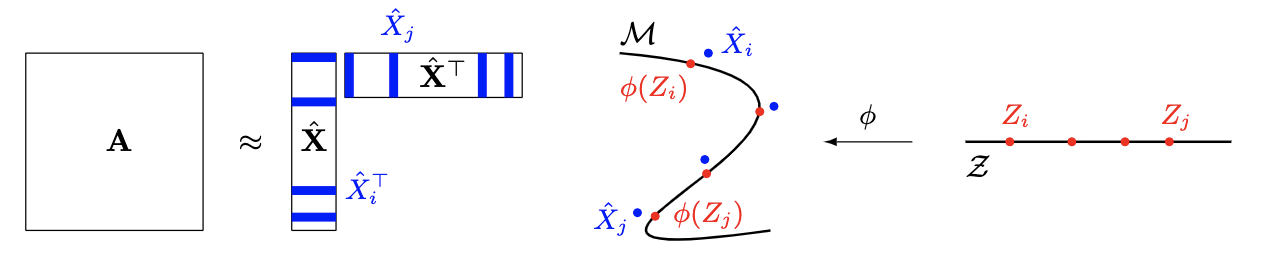
Figure 1: Illustration of theory in the case $d=1$. Our analysis reveals how geodesic distance, along $\mathcal{M}$, between $\phi(Z_{i})$ and $\phi(Z_{j})$, is related to geodesic distance, along $\mathcal{Z}$, between $Z_{i}$ and $Z_{j}$.

2.1 Spectral embedding, as estimating $\phi(Z_{i})$

In our mathematical setup (precise details come later) the kernel $f$ will be nonnegative definite and $\phi$ will be the associated Mercer feature map. It is well known that each point $\phi(Z_{i})$ then lives in an infinite-dimensional Hilbert space, which will be denoted $\ell_{2}$, and the inner-product $\langle\phi(Z_{i}),\phi(Z_{j})\rangle_{2}$ in this space equals $f(Z_{i},Z_{j})$.

The spectral embedding procedure. For $p\leq n$, we define the $p$-dimensional spectral embedding of $\mathbf{A}$ to be $\hat{\mathbf{X}}=[\hat{X}_{1},\ldots,\hat{X}_{n}]^{\top}=\hat{\mathbf{U}}|\hat{\mathbf{S}}|^{1/2}\in\mathbb{R}^{n\times p}$, where $|\hat{\mathbf{S}}|\in\mathbb{R}^{p\times p}$ is a diagonal matrix containing the absolute values of the $p$ largest eigenvalues of $\mathbf{A}$, by magnitude, and $\hat{\mathbf{U}}\in\mathbb{R}^{n\times p}$ is a matrix containing corresponding orthonormal eigenvectors, in the same order. The R packages irlba and RSpectra provide fast solutions which can exploit sparse inputs.

One should think of $\hat{X}_{i}$ as approximating the vector of first $p$ components of $\phi(Z_{i})$, denoted $\phi_{p}(Z_{i})$, up to orthogonal transformation, and this can be formalised to a greater or lesser extent depending on what assumptions are made. There are several situations, e.g. $f$ any polynomial [45], the cosine kernel used in Section 4.1, the degree-corrected [29] or mixed-membership [6] stochastic block model, in which only the first $p_{0}$ (say) components of $\phi(\cdot)$ are nonzero, where typically $p_{0}\geq d$. If, after $n$ reaches $p_{0}$, we embed into $p=p_{0}$ dimensions, then with $\|\cdot\|$ denoting the Euclidean norm, we have [18]:

$$\max_{i\in\{1,\ldots,n\}}\lVert\mathbf{Q}\hat{X}_{i}-\phi_{p}(Z_{i})\rVert=O_{\mathbb{P}}\left(\tfrac{(\log n)^{c}}{n^{1/2}}\right),$$ (2)

for a universal constant $c\geq 1$, orthogonal matrix $\mathbf{Q}$, under regularity assumptions on the $Z_{i}$’s, $f$ and $\mathbf{E}$ (that $Z_{i}$ are i.i.d., $f(Z_{i},Z_{j})$ has finite expectation, and the perturbations $\mathbf{E}^{ij}$ are independent and centered with exponential tails). This encompasses the case where $\mathbf{A}$ is binary, for example a graph adjacency matrix [36, 46]. Similar results are available in the cases where $\mathbf{A}$ is a Laplacian [46, 40] or covariance matrix [17]. The methods of this paper are based, in practice, on the distances $\lVert\hat{X}_{i}-\hat{X}_{j}\rVert$, which are invariant to orthogonal transformation and so for the purposes of validating $\lVert\hat{X}_{i}-\hat{X}_{j}\rVert\approx\lVert\phi_{p}(Z_{i})-\phi_{p}(Z_{j})\rVert$ the presence of $\mathbf{Q}$ in (2) is immaterial.

For $\hat{X}_{i}$ to converge to $\phi(Z_{i})$ more generally, we must let its dimension $p$ grow with $n$ and, at least given the present state of literature, accept weaker consistency results, for example, convergence in Wasserstein distance between $\mathbf{Q}\hat{X}_{1},\ldots\mathbf{Q}\hat{X}_{n}$ and $\phi_{p}(Z_{1}),\ldots,\phi_{p}(Z_{n})$ [32]. Uniform consistency results, in the style of (2), are also available for indefinite [46], bipartite, and directed graphs [25]. These are left for future work because of the complications of $\mathbf{Q}$ no longer being orthogonal.

Rank selection. In real data, where $n$ is typically fixed, there is no ‘best’ way of selecting $p$, as discussed for example in [42]. The method of [65], based on profile-likelihood, provides a popular, practical choice, taking as input the spectrum of $\mathbf{A}$, and is implemented in the R package igraph.

2.2 Isomap, as estimating $Z_{i}$

We propose to recover $Z_{1},\ldots,Z_{n}$ through the following procedure.

Algorithm 1 Isomap procedure

1:input $p$-dimensional points $\hat{X}_{1},\ldots,\hat{X}_{n}$

2:Compute the neighbourhood graph of radius $\epsilon$: a weighted graph connecting $i$ and $j$, with weight $\|\hat{X}_{i}-\hat{X}_{j}\|$, if $\|\hat{X}_{i}-\hat{X}_{j}\|\leq\epsilon$

3:Compute the matrix of shortest paths on the neighbourhood graph, $\hat{\mathbf{D}}_{\mathcal{M}}\in\mathbb{R}^{n\times n}$

4:Apply classical multidimensional scaling (CMDS) to $\hat{\mathbf{D}}_{\mathcal{M}}$ into $\mathbb{R}^{d}$

5:return $d$-dimensional points $\hat{Z}_{1},\ldots,\hat{Z}_{n}$

Theorem 1 below establishes, under general assumptions, that $\mathcal{M}\coloneqq\phi(\mathcal{Z})$ is a topological manifold of Hausdorff dimension exactly that of $\mathcal{Z}$ (as opposed to an upper bound [45]). It also proposes a ‘change of metric’, often trivial, under which a path on $\mathcal{Z}$ and its image on $\mathcal{M}$ have the same length.

This result explains how $\hat{Z}_{1},\ldots,\hat{Z}_{n}$ can estimate $Z_{1},\dots,Z_{n}$. First, think of a path from $\hat{X}_{i}$ to $\hat{X}_{j}$ on the neighbourhood graph as a noisy, discrete version of some corresponding continuous path from $\phi(Z_{i})$ to $\phi(Z_{j})$ on $\mathcal{M}$. The length of the first (the sum of the weights of the edges) is approximately equal to the length of the second if measured in the standard metric: an infinitesmal step from $x$ to $x+\mathrm{d}x$ has length $\smash{\langle\mathrm{d}x,\mathrm{d}x\rangle_{2}^{1/2}}$. By inversion of $\phi$ we can trace a third path, taking us from $Z_{i}$ to $Z_{j}$ on $\mathcal{Z}$. But to make its length agree with the first two, we must pick a non-standard metric: an infinitesmal step from $z$ to $z+\mathrm{d}z$ must be regarded to have length $\langle\mathrm{d}z,\mathbf{H}_{z}\mathrm{d}z\rangle^{1/2}=\sqrt{\mathrm{d}z^{\top}\mathbf{H}_{z}\mathrm{d}z}$, where

$$\mathbf{H}_{z}^{ij}\coloneqq\left.\dfrac{\partial^{2}f}{\partial x^{(i)}\partial y^{(j)}}\right|_{(z,z)},\quad i,j\in\{1,\ldots,d\}.$$

The exciting news for practical purposes is that, through elementary calculus, we might establish that $\mathbf{H}_{z}$ is constant in $z$ (e.g. if $f$ is translation-invariant) or even proportional to the identity (e.g. if $f$ is just a function of Euclidean distance). In the latter case, if $\mathcal{Z}$ is convex, it is not too difficult to see that the length of the shortest path, from $\phi(Z_{i})$ to $\phi(Z_{j})$ on $\mathcal{M}$, must be proportional to the Euclidean distance between $Z_{i}$ and $Z_{j}$. Thus, the matrix of shortest paths obtained by Isomap (Step 2) approximates the matrix of Euclidean distances between the $Z_{i}$ (up to scaling), from which the $Z_{i}$ themselves can be recovered (Step 3), up to scaling, rotation, and translation. Of course, we have taken a few liberties in this argument, such as assuming $\phi$ to be invertible and $\mathrm{d}z^{\top}\mathbf{H}_{z}\mathrm{d}z$ to be positive. We will address these rigorously in the next section.

Dimension and radius selection. For visualisation in our examples we will pick $d=1$ or $d=2$. For other applications, $d$ can be estimated as the approximate rank of $\hat{\mathbf{D}}_{\mathcal{M}}$ after double-centering [60], e.g. via [65], again. In practice, we suggest picking $\epsilon$ just large enough for the neighbourhood graph to be connected or, if the data have outliers, a fixed quantile (such as 5%) of $\hat{\mathbf{D}}_{\mathcal{M}}$, removing nodes outside the largest connected component. The same recommendations apply if the $k$-nearest neighbour graph is used instead of the $\epsilon$-neighbourhood graph.

3 Theory

3.1 Setup and assumptions

The usual inner-product and Euclidean norm on $\mathbb{R}^{d}$ are denoted $\left\langle\cdot,\cdot\right\rangle$ and $\|\cdot\|$. $\ell_{2}$ is the set of $x=[x^{(1)}\,x^{(2)}\,\cdots]^{\top}\in\mathbb{R}^{\mathbb{N}}$ such that $\|x\|_{2}\coloneqq(\sum_{k=1}^{\infty}|x^{(k)}|^{2})^{1/2}<\infty$. For $x,y\in\ell_{2}$ , $\left\langle x,y\right\rangle_{2}\coloneqq\sum_{k=1}^{\infty}x^{(k)}y^{(k)}$. With $d\geq 1$, let $\mathcal{Z}$ be a compact subset of $\mathbb{R}^{d}$, and let $\widetilde{\mathcal{Z}}$ be a closed ball in $\mathbb{R}^{d}$, centered at the origin, such that $\mathcal{Z}\subset\widetilde{\mathcal{Z}}$. Let $f:\widetilde{\mathcal{Z}}\times\widetilde{\mathcal{Z}}\to\mathbb{R}$ be a symmetric, continuous, nonnegative-definite function.

By Mercer’s Theorem, e.g., [51, Thm 4.49], there exist nonnegative real numbers $(\lambda_{k})_{k\geq 1}$ and functions $(u_{k})_{k\geq 1}$, with each $u_{k}:\widetilde{\mathcal{Z}}\to\mathbb{R}$, which are orthonormal with respect to the inner-product $(u_{j},u_{k})\mapsto\int_{\tilde{\mathcal{Z}}}u_{j}(x)u_{k}(x)\mathrm{d}x$

and such that

$$f(x,y)=\sum_{k=1}^{\infty}\lambda_{k}u_{k}(x)u_{k}(y),\quad x,y\in\widetilde{\mathcal{Z}},$$ (3)

where the convergence is absolute and uniform. For $x\in\mathcal{Z}$ let $\phi(x)\coloneqq[\lambda_{1}^{1/2}u_{1}(x)\;\lambda_{2}^{1/2}u_{2}(x)\;\cdots]^{\top}\in\mathbb{R}^{\mathbb{N}}$. The image of $\mathcal{Z}$ by $\phi$ is denoted $\mathcal{M}$. Observe from (3) that for any $x,y\in\mathcal{Z}$, $f(x,y)=\left\langle\phi(x),\phi(y)\right\rangle_{2}$ , $\|\phi(x)\|_{2}^{2}=f(x,x)$, and the latter is finite for any $x\in\mathcal{Z}$ since $f$ is continuous and $\mathcal{Z}$ is compact, hence $\mathcal{M}\subset\ell_{2}$.

The following definitions are standard in metric geometry [16]. For any $a,b\in\ell_{2},$ a path in $\mathcal{M}$ with end-points $a,b$ is a continuous function $\gamma:[0,1]\to\mathcal{M}$ such that $\gamma_{0}=a$ and $\gamma_{1}=b$. With $n\geq 1$, a non-decreasing sequence $t_{0},\ldots,t_{n}$ such that $t_{0}=0$ and $t_{n}=1$, is called a partition. Given a path $\gamma$ and a partition $\mathcal{P}=(t_{0},\ldots,t_{n})$, define $\chi(\gamma,\mathcal{P})\coloneqq\sum_{k=1}^{n}\|\gamma_{t_{k}}-\gamma_{t_{k-1}}\|_{2}$. The length of $\gamma$ (w.r.t. $\|\cdot\|_{2}$) is $l(\gamma)\coloneqq\sup_{\mathcal{P}}\chi(\gamma,\mathcal{P})$, where the supremum is over all possible partitions. The geodesic distance in $\mathcal{M}$ between $a$ and $b$ is defined to be the infimum of $l(\gamma)$ over all paths $\gamma$ in $\mathcal{M}$ with end-points $a,b$. $\mathbf{D}_{\mathcal{M}}^{ij}$ denotes geodesic distance in $\mathcal{M}$ between $\phi(Z_{i})$ and $\phi(Z_{j})$. Similarly a path $\eta$ in $\mathcal{Z}$ with end-points $x,y$ is a continuous function $\eta:[0,1]\to\mathcal{Z}$ such that $\eta_{0}=x,\eta_{1}=y$, and with $\chi(\eta,\mathcal{P})\coloneqq\sum_{k=1}^{n}\|\eta_{t_{k}}-\eta_{t_{k-1}}\|$ the length of $\eta$ (w.r.t. $\|\cdot\|$) is $l(\eta)\coloneqq\sup_{\mathcal{P}}\chi(\eta,\mathcal{P})$. $\mathbf{D}_{\mathcal{Z}}^{ij}$ denotes geodesic distance in $\mathcal{Z}$ between $Z_{i}$ and $Z_{j}$. If $\mathcal{Z}$ is convex, $\mathbf{D}_{\mathcal{Z}}^{ij}=\|Z_{i}-Z_{j}\|$.

Assumption 1.

For all $x,y\in\mathcal{Z}$ with $x\neq y$, there exists $a\in\mathcal{Z}$ such that $f(x,a)\neq f(y,a)$.

Assumption 2.

f is $C^{2}$ on $\widetilde{\mathcal{Z}}$ and for every $z\in\mathcal{Z}$, the matrix $\mathbf{H}_{z}$ is positive definite.

Assumption 1 is used to show $\phi$ is injective. Assumption 2 has various implications, loosely speaking it ensures a non-degenerate relationship between path-length in $\mathcal{M}$ and path-length in $\mathcal{Z}$. Concerning our general setup, if $f$ is not required to be nonnegative definite, but is still symmetric, then a representation formula like (3) is available under e.g. trace-class assumptions [45]. It is of interest to generalise our results to that scenario but technical complications are involved, so we leave it for future research.

3.2 Path-lengths in $\mathcal{M}$ and in $\mathcal{Z}$

Theorem 1.

Let assumptions 1 and 2 hold. Then $\phi$ is a bi-Lipschitz homeomorphism between $\mathcal{Z}$ and $\mathcal{M}$. Let $a,b$ be any two points in $\mathcal{M}$ such that there exists a path in $\mathcal{M}$ with end-points $a,b$ of finite length. Let $\gamma$ be any such path and define $\eta:[0,1]\to\mathcal{Z}$ by $\eta_{t}\coloneqq\phi^{-1}(\gamma_{t})$. Then $\eta$ is a path in $\mathcal{Z}$ with $l(\eta)<\infty$. For any $\epsilon>0$ there exists a partition $\mathcal{P}_{\epsilon}$ such that for any partition $\mathcal{P}=(t_{0},\ldots,t_{n})$ satisfying $\mathcal{P}_{\epsilon}\subseteq\mathcal{P}$,

$$\left|l(\gamma)-\sum_{k=1}^{n}\left\langle\eta_{t_{k}}-\eta_{t_{k-1}},\mathbf{H}_{\eta_{t_{k-1}}}(\eta_{t_{k}}-\eta_{t_{k-1}})\right\rangle^{1/2}\right|\leq\epsilon.$$ (4)

If $\gamma$ and $\eta$ are continuously differentiable, the following two equalities hold:

$$l(\gamma)=\int_{0}^{1}\|\dot{\gamma}_{t}\|_{2}\mathrm{d}t=\int_{0}^{1}\left\langle\dot{\eta}_{t},\mathbf{H}_{\eta_{t}}\dot{\eta}_{t}\right\rangle^{1/2}\mathrm{d}t.$$ (5)

The proof is in the appendix. In the terminology of differential geometry, the collection of inner-products $(x,y)\mapsto\left\langle x,\mathbf{H}_{z}y\right\rangle$, indexed by $z\in\mathcal{Z}$, constitute a Riemannian metric on $\mathcal{Z}$, see e.g. [41, Ch.1 and p.121] for background, and the right hand side of (5) is the length of the path $\eta$ in $\mathcal{Z}$ with respect to this Riemannian metric. The theorem tells us that finding geodesic distance in $\mathcal{M}$, i.e. minimising $l(\gamma)$ with respect to $\gamma$ for fixed end-points say $a=\phi(Z_{i}),b=\phi(Z_{j})$, is equivalent to minimizing path-length in $\mathcal{Z}$ between end-points $\phi^{-1}(a)=Z_{i},\phi^{-1}(b)=Z_{j}$ under the Riemannian metric. In section 3.3 we will show how, for various classes of kernels, this minimisation can be performed in closed form leading to explicit relationships between $\mathbf{D}_{\mathcal{M}}^{ij}$ and $\mathbf{D}_{\mathcal{Z}}^{ij}$. In Section 3.3 we focus on (5) rather than (4) only for ease of exposition, it is shown in the appendix that exactly the same conclusions can be derived directly from (4). To avoid repetition Assumption 1 will be taken to hold throughout section 3.3 without further mention.

3.3 Geodesic distance in $\mathcal{M}$ and in $\mathcal{Z}$

Translation invariant kernels. Suppose $\mathcal{Z}\subset{\mathbb{R}^{d}}$ is compact and convex, and $f(x,y)=g(x-y)$ where $g:\mathbb{R}^{d}\to\mathbb{R}$ is $C^{2}$. In this situation $\mathbf{H}_{z}$ is constant in $z$, and equal to the Hessian of $-g$ evaluated at the origin. The positive-definite part of Assumption 2 is therefore satisfied if and only if $g$ has a local maximum at the origin. We now use Theorem 1 to find geodesic distance in $\mathcal{M}$ between generic points $a,b\in\mathcal{M}$ for this class of translation-invariant kernels. To do this we obtain a lower bound on $l(\gamma)$ over all paths $\gamma$ in $\mathcal{M}$ with end-points $a,b$, then show there exists such a path whose length achieves this lower bound.

Let $\mathbf{G}=\mathbf{V}\mathbf{\Lambda}^{1/2}$ where $\mathbf{V}\mathbf{\Lambda}\mathbf{V}^{\top}$ is the eigendecomposition of the Hessian of $-g$ evaluated at the origin, so $\mathbf{H}_{z}=\mathbf{G}\mathbf{G}^{\top}$ for all $z$. Then from (5), for a generic path $\gamma$ in $\mathcal{M}$ with end-points $a,b$,

$$l(\gamma) =\int_{0}^{1}\left\langle\dot{\eta}_{t},\mathbf{H}_{\eta_{t}}\dot{\eta}_{t}\right\rangle^{1/2}\mathrm{d}t=\int_{0}^{1}\left\langle\dot{\eta}_{t},\mathbf{G}\mathbf{G}^{\top}\dot{\eta}_{t}\right\rangle^{1/2}\mathrm{d}t=\int_{0}^{1}\|\mathbf{G}^{\top}\dot{\eta}_{t}\|\mathrm{d}t$$ (6)

$$\geq\left\|\int_{0}^{1}\mathbf{G}^{\top}\dot{\eta}_{t}\mathrm{d}t\right\|=\left\|\mathbf{G}^{\top}\int_{0}^{1}\dot{\eta}_{t}\mathrm{d}t\right\|=\|\mathbf{G}^{\top}(\eta_{1}-\eta_{0})\|=\|\mathbf{G}^{\top}[\phi^{-1}(b)-\phi^{-1}(a)]\|,$$ (7)

where the inequality is due to the triangle inequality for the $\|\cdot\|$ norm. The right-most term in (7) is independent of $\gamma$, other than through the end-points $a,b.$ To see there exists a path whose length equals this lower bound, take

$$\tilde{\eta}_{t}\coloneqq\phi^{-1}(a)+t[\phi^{-1}(b)-\phi^{-1}(a)],\quad t\in[0,1],$$ (8)

which is well-defined as a path in $\mathcal{Z}$, since for this class of kernels $\mathcal{Z}$ is assumed convex. With $\tilde{\gamma}_{t}\coloneqq\phi(\tilde{\eta}_{t})$, $\tilde{\gamma}$ is clearly a path in $\mathcal{M}$. Differentiating $\tilde{\eta}_{t}$ w.r.t. $t$ and substituting into (6) shows $l(\tilde{\gamma})=\|\mathbf{G}^{\top}[\phi^{-1}(b)-\phi^{-1}(a)]\|$, as required. The following proposition summarises our conclusions in the case that $a=\phi(Z_{i})$ and $b=\phi(Z_{j})$, for any $Z_{i},Z_{j}$.

Proposition 1.

If $\mathcal{Z}$ is compact and convex, and $f(x,y)=g(x-y)$ where $g:\mathbb{R}^{d}\to\mathbb{R}$ is $C^{2}$ and has a local maximum at the origin, then $\mathbf{D}_{\mathcal{M}}^{ij}$ is equal to Euclidean distance between $Z_{i}$ and $Z_{j}$, up to their linear transformation by $\mathbf{G}^{\top}$. In the particular case where $g(x-y)=h(\|x-y\|^{2})$ with $h^{\prime}(0)<0$, we have $\mathbf{D}_{\mathcal{M}}^{ij}\propto\mathbf{D}_{\mathcal{Z}}^{ij}=\|Z_{i}-Z_{j}\|$.

Inner-product kernels. Suppose $\mathcal{Z}=\{x\in\mathbb{R}^{d}:\|x\|=1\}$ and $f(x,y)=g(\left\langle x,y\right\rangle)$, where $g:\mathbb{R}\to\mathbb{R}$ is $C^{2}$ and such that $g^{\prime}(1)>0$. In this case $\mathbf{H}_{z}=g^{\prime}(1)\mathbf{I}+g^{\prime\prime}(1)zz^{\top}$, and by a result of [27], any kernel of the form $f(x,y)=g(\left\langle x,y\right\rangle)$ on the sphere is positive-definite iif $g(x)=\sum_{n=0}^{\infty}a_{n}x^{n}$ for some nonnegative $(a_{n})_{n\geq 0}$, implying $g^{\prime\prime}(1)\geq 0$. Assumption 2 then holds. To derive the geodesic distance in $\mathcal{M}$, first write out (5) for a generic path $\gamma$ in $\mathcal{M}$ with end-points $a,b$:

$$l(\gamma)=\int_{0}^{1}\left\langle\dot{\eta}_{t},\mathbf{H}_{\eta_{t}}\dot{\eta}_{t}\right\rangle^{1/2}\mathrm{d}t=\int_{0}^{1}\left(g^{\prime}(1)\|\dot{\eta}_{t}\|^{2}+g^{\prime\prime}(1)\left|\left\langle\eta_{t},\dot{\eta}_{t}\right\rangle\right|^{2}\right)^{1/2}\mathrm{d}t.$$ (9)

Since $\mathcal{Z}$ is a radius-$1$ sphere centered at the origin we must have $\|\eta_{t}\|=1$ for all $t$, so $0=\frac{1}{2}\frac{\mathrm{d}}{\mathrm{d}t}\|\eta_{t}\|^{2}=\frac{1}{2}\frac{\mathrm{d}}{\mathrm{d}t}\left\langle\eta_{t},\eta_{t}\right\rangle=\left\langle\eta_{t},\dot{\eta}_{t}\right\rangle$. Therefore the r.h.s. of (9) is in fact equal to $g^{\prime}(1)^{1/2}\int_{0}^{1}\|\dot{\eta}_{t}\|\mathrm{d}t$. This is minimised over all possible paths $\eta$ in $\mathcal{Z}$ with end-points $\phi^{-1}(a),\phi^{-1}(b)$ when $\eta$ is a shortest (with respect to Euclidean distance) circular arc in $\mathcal{Z}$, in which case $\int_{0}^{1}\|\dot{\eta}_{t}\|\mathrm{d}t=\arccos\left\langle\phi^{-1}(a),\phi^{-1}(b)\right\rangle$. Thus we have:

Proposition 2.

If $\mathcal{Z}=\{x\in\mathbb{R}^{d}:\|x\|=1\}$ and $f(x,y)=g(\left\langle x,y\right\rangle)$ where $g:\mathbb{R}\to\mathbb{R}$ is $C^{2}$ and such that $g^{\prime}(1)>0$, then $\mathbf{D}_{\mathcal{M}}^{ij}=g^{\prime}(1)^{1/2}\mathbf{D}_{\mathcal{Z}}^{ij}=g^{\prime}(1)^{1/2}\arccos\left\langle Z_{i},Z_{j}\right\rangle$.

Additive kernels. Suppose $\mathcal{Z}$ is the Cartesian product of intervals $\mathcal{Z}_{i}=[c_{i}^{-},c_{i}^{+}]$, $i=1,\ldots,d$ and $f(x,y)=\sum_{i=1}^{d}\alpha_{i}f_{i}(x^{(i)},y^{(i)})$, $x=[x^{(1)}\,\cdots\,x^{(d)}]^{\top}$, where each $\alpha_{i}>0$ and each $f_{i}$ is positive-definite and $C^{2}$. For this class of kernels $\mathbf{H}_{z}$ is diagonal with $\mathbf{H}_{z}^{ii}=\alpha_{i}\left.\frac{\partial^{2}f_{i}}{\partial x^{(i)}\partial y^{(i)}}\right|_{(z^{(i)},z^{(i)})}$ where $z^{(i)}$ is the $i$th element of the vector $z$. The positive-definite part of Assumption 2 thus holds if these diagonal elements are strictly positive for all $z\in\mathcal{Z}$.

Let us introduce the vector of monotonically increasing transformations:

$$\quad\psi(z)\coloneqq[\psi_{1}(z^{(1)})\,\cdots\,\psi_{d}(z^{(d)})]^{\top},\qquad\;\psi_{i}(z^{(i)})\coloneqq\alpha_{i}^{1/2}\int_{c_{i}^{-}}^{z^{(i)}}\left.\frac{\partial^{2}f_{i}}{\partial x^{(i)}\partial y^{(i)}}\right|_{(\xi,\xi)}^{1/2}\mathrm{d}\xi,$$ (10)

and write the vector of corresponding inverse transformations $\psi^{-1}$. For a generic path $\gamma$ in $\mathcal{M}$ with end-points $a,b$ and as usual $\eta_{t}\coloneqq\phi^{-1}(\gamma_{t})$, define $\zeta_{t}\coloneqq\psi(\eta_{t})$. Then:

$$l(\gamma)=\int_{0}^{1}\left\langle\dot{\eta}_{t},\mathbf{H}_{\eta_{t}}\dot{\eta}_{t}\right\rangle^{1/2}\mathrm{d}t =\int_{0}^{1}\|\dot{\zeta}_{t}\|\mathrm{d}t$$ (11)

$$\geq\left\|\int_{0}^{1}\dot{\zeta}_{t}\,\mathrm{d}t\right\|=\|\zeta_{1}-\zeta_{0}\|=\|\psi\circ\phi^{-1}(b)-\psi\circ\phi^{-1}(a)\|,$$ (12)

where the second and last equalities hold due to the definition of $\zeta_{t}$, and $\circ$ denotes elementwise composition. The quantity $\|\psi\circ\phi^{-1}(b)-\psi\circ\phi^{-1}(a)\|$ is thus a lower bound on path-length $l(\gamma)$ for any path $\gamma$ in $\mathcal{M}$ with end-points $a,b$. To see that there exists a path whose length achieves this lower bound, and hence that it is the geodesic distance in $\mathcal{M}$ between $a,b$, define $\tilde{\gamma}_{t}\coloneqq\phi\circ\psi^{-1}(\tilde{\zeta}_{t})$ where $\tilde{\zeta}_{t}\coloneqq\psi\circ\phi^{-1}(a)+t[\psi\circ\phi^{-1}(b)-\psi\circ\phi^{-1}(a)]$. Differentiating $\tilde{\zeta}_{t}$ w.r.t. $t$ and substituting into (11) yields $l(\tilde{\gamma})=\|\psi\circ\phi^{-1}(b)-\psi\circ\phi^{-1}(a)\|$, as required. Our conclusions in the case that $a=\phi(Z_{i})$ and $b=\phi(Z_{j})$ are summarised by:

Proposition 3.

If $\mathcal{Z}$ is the Cartesian product of $d$ intervals $\mathcal{Z}_{i}\subset{\mathbb{R}}$, $i=1,\ldots,d$, and $f(x,y)=\sum_{i=1}^{d}\alpha_{i}f_{i}(x^{(i)},y^{(i)})$ where for each $i$, $\alpha_{i}>0$, $f_{i}$ is positive definite and $C^{2}$, and $\left.\frac{\partial^{2}f_{i}}{\partial x^{(i)}\partial y^{(i)}}\right|_{(z,z)}>0$ for all $z\in\mathcal{Z}_{i}$, then $\mathbf{D}_{\mathcal{M}}^{ij}$ is equal to the Euclidean distance between $Z_{i}$ and $Z_{j}$ up to their coordinatewise-monotone transformation by $\psi$. If $\left.\alpha_{i}\frac{\partial^{2}f_{i}}{\partial x^{(i)}\partial y^{(i)}}\right|_{(z,z)}$ is a positive constant over all $z\in\mathcal{Z}_{i}$, and over all $i=1,\ldots,d$, then $\mathbf{D}_{\mathcal{M}}^{ij}\propto\mathbf{D}_{\mathcal{Z}}^{ij}=\|Z_{i}-Z_{j}\|$.

4 Experiments

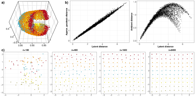
Figure 2: Simulated data example. a) Spectral embedding (first 3 dimensions), b) comparison of latent, approximate geodesic, and ambient distance and c) latent position recovery in the dense regime by spectral embedding followed by Isomap for increasing $n$. To aid visualisation, all plots in c) display a subset of $100$ estimated positions corresponding to true positions on a sub-grid which is common across $n$. Estimated positions are coloured according to their true $y$-coordinate.

4.1 Simulated data: latent position network model

This section shows the theory at work in a pedagogical example, where $\mathbf{A}$ is an adjacency matrix. Consider an undirected random graph following a latent position model with kernel $f(x,y)=\rho_{n}\{\cos(x^{(1)}-y^{(1)})+\cos(x^{(2)}-y^{(2)})+2\}/4$, operating on $\mathbb{R}^{2}\times\mathbb{R}^{2}$. Here, the sequence $\rho_{n}$ is a sparsity factor which will either be constant, $\rho_{n}=1$, or shrinking to zero sufficiently slowly, reflecting dense (degree grows linearly) and sparse (degree grows sublinearly) regimes respectively. The kernel is clearly translation-invariant, satisfies Assumptions 1 and 2 and has finite rank, $p=5$. The true latent positions $Z_{i}\in\mathbb{R}^{2}$ are deterministic and equally spaced points on a grid over the region $\mathcal{Z}=[-\pi+0.25,\pi-0.25]\times[-\pi+0.25,\pi-0.25]$, this range chosen to give valid probabilities and an interesting bottleneck in the 2-dimensional manifold $\mathcal{M}$. From Proposition 1, the geodesic distance between $\phi(Z_{i})$ and $\phi(Z_{j})$ on $\mathcal{M}$ is equal to the Euclidean distance between $Z_{i}$ and $Z_{j}$, up to scaling, specifically $\mathbf{D}_{\mathcal{M}}^{ij}=\rho_{n}\mathbf{D}^{ij}_{\mathcal{Z}}/2$.

Focusing first on the dense regime, for each $n=100,400,1600,6400$, we simulate a graph, and its spectral embedding $\hat{X}_{1},\ldots,\hat{X}_{n}$ into $p=5$ dimensions. The first three dimensions of this embedding are shown in Figure 2a), and we see that the points gather about a two-dimensional, curved, manifold. To approximate geodesic distance, we compute a neighbourhood graph of radius $\epsilon$ from $\hat{X}_{1},\ldots,\hat{X}_{n}$, choosing $\epsilon$ as small as possible subject to maintaining a connected graph. Figure 2b) shows that approximated geodesic distances roughly agree with the true Euclidean distances in latent space $\mathcal{Z}$ (up to the predicted scaling of 1/2), whereas there is significant distortion between ambient and latent distance ($\lVert\hat{X}_{i}-\hat{X}_{j}\rVert$ versus $\lVert Z_{i}-Z_{j}\rVert$). Finally, we recover the estimated latent positions in $\mathbb{R}^{2}$ using Isomap, which we align with the original by Procrustes (orthogonal transformation with scaling), in Figure 2c). As the theory predicts, the recovery error vanishes as $n$ increases.

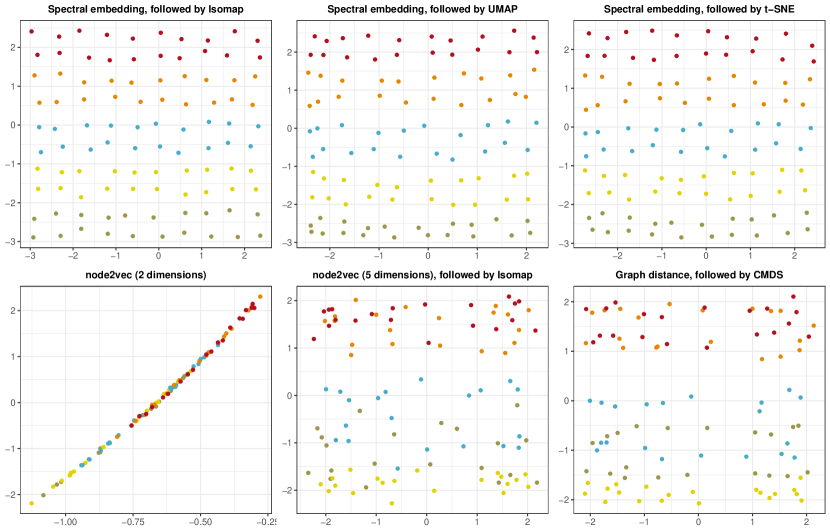
Figure 6: Latent position recovery in a sparse regime using different combinations of techniques with $n=6400$. The first row contains spectral embedding followed by different nonlinear dimension reduction techniques and the second row contains node2vec, node2vec followed by Isomap, and we have attempted recovery using graph distances [11]. To aid visualisation, all plots will display a subset of $100$ on a fixed sub-grid, coloured according to their true location.

In the appendix, we perform the same experiment in a sparse regime, $n\rho_{n}=\omega\{\log^{4}n\}$, chosen to ensure the spectral embedding is still consistent, and the recovery error still shrinks, but more slowly. We also implement other related approaches: UMAP, t-SNE applied to spectral embedding, node2vec directly into two dimensions and node2vec in five dimensions followed by Isomap (Figure 6). We use default configurations for all other hyperparameters. Together, the results support the central recommendation of this paper: to use matrix factorisation (e.g. spectral embedding, node2vec), followed by nonlinear dimension reduction (e.g. Isomap, UMAP, t-SNE).

4.2 Real data: the global flight network

For this example, we use a publically available, clean version [52] (with license details therein) of the crowdsourced OpenSky dataset. Six undirected graphs are extracted, for the months November 2019 to April 2020, connecting any two airports in the world for which at least a single flight was recorded ($n\approx 10,000$ airports in each). For each graph the adjacency matrix $\mathbf{A}$ is spectrally embedded into $p=10$ dimensions, degree-corrected by spherical projection [35, 33, 49], after which we apply Isomap with $\epsilon$ chosen as the 5% distance quantile.

The dimension $p$ was chosen as a loose upper bound on the dimension estimate returned by the method of [65] on any of the individual graphs, as to facilitate comparison we prefer to use the same dimension throughout (e.g. to avoid artificial differences in variance) and so follow the recommendation of [12] to err on the large side (experiments with different choices of $p$ are in the appendix). In the degree-correction step we aim to remove network effects related to “airport popularity” (e.g. population, economic and airport size), after which geographic distance might be expected to be the principal factor deciding whether there should be a flight between two airports. Therefore, after applying Isomap, we might hope that $\hat{Z}_{i}$ could estimate the geographical location of airport $i$. The experiments take a few hours on a standard desktop (and the same is a loose upper bound on compute time for the other experiments in the paper).

The embedding for January is shown in Figures 3)a-b), before and after Isomap. Both recover real geographic features, notably the relative positioning of London, Paris, Madrid, Lisbon, Rome. However, the embedding of the US is warped, and only after using Isomap do we see New York and Los Angeles correctly positioned at opposite extremes of the country. As further confirmation, Figures 3)c-d) show the results restricted to North America, with the points coloured by latitude and longitude. For this continent, the accuracy of longitude recovery is particularly striking.

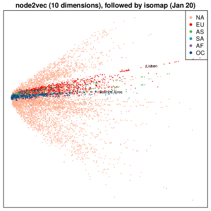
Figure 10: Visualisation of the global flight network. Node2vec into 20 dimensions followed by Isomap. The colours indicate continents (NA = North America, EU = Europe, AS = Asia, AF = Africa, OC = Oceania) and a spread of cities with high-traffic airports are labelled.

In line with the recommendation to overestimate $p$ [12], one obtains a similar figure using $p=20$ before applying Isomap (Figure 10, appendix), whereas the corresponding figure with $p=2$ is too poor to show.

In the appendix, the embeddings of all six months are shown, aligned using two-dimensional Procrustes, showing an important structural change in April. A statistical analysis of inter-continental geodesic distances suggests the change reflects severe flight restrictions in South America and Africa, at the beginning COVID-19 pandemic (the 11th March 2020 according to the WHO).

Figure 3: Visualisation of the global flight network, January 2020. a) Spectral embedding, b) spectral embedding followed by Isomap, colours indicating continents (NA = North America, EU = Europe, AS = Asia, AF = Africa, OC = Oceania), c-d) the same restricted to North America, showing only the airports within the continent’s 5%-95% inter-quantile range of longitude and latitude, colours indicating the longitude (c) and latitude (d) of the airports.

4.3 Real data: correlations between daily temperatures around the globe

In this example $\mathbf{A}$ is a correlation matrix and we demonstrate a simple model-checking diagnostic informed by our theory. The raw data consist of average temperatures over each day, for several thousand days, recorded in cities around the globe. These data are open source, originate from Berkeley Earth [1] and the particular data set analyzed is from [3]. We used open source latitude and longitude data from [4]. See those references for license details. Removing cities and dates for which data are missing yields a temperature time-series of $1450$ common days for each of the $n=2211$ cities. $\mathbf{A}$ is the matrix of Pearson correlation coefficients between the $n$ time-series.

Figure 4b) shows the spectral embedding of $\mathbf{A}$, with $p=2$ and points coloured by the latitude of the corresponding cities. Two visual features are striking: the concentration of points around a curved manifold, and a correspondence between latitude and location on the manifold. Figure 4c) shows latitude against estimated latent positions from Isomap using the $k$-nearest neighbour graph with $k=200$, which is roughly $10\%$ of $n$, and with $d=1$. A clear monotone relationship appears. Our theoretical results can explain this phenomenon. Notice that when $d=1$, the additive structure of the kernel in Proposition 3 disappears. Hence Proposition 3 shows that in the case $d=1$, for any kernel (meeting the basic requirements of section 3.1, including Assumptions 1 and 2 of course) $\mathbf{D}_{\mathcal{M}}^{ij}$ is equal to Euclidean distance between $Z_{i}$ and $Z_{j}$ up to their monotone transformation by $\psi$ defined in (10). In turn, this implies that if $\mathbf{A}$ did actually follow the model (1) for some $f$ and some “true” latent positions $Z_{1},\ldots,Z_{n}$ to which we had access, we should observe a monotone relationship between those true latent positions and the estimated positions $\hat{Z}_{1},\ldots,\hat{Z}_{n}$ from Isomap.

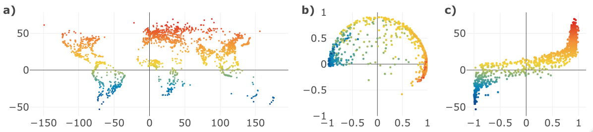
Figure 4: Temperature correlation example. a) Locations in degrees latitude and longitude of cities where temperatures were recorded, b) spectral embedding with $p=2$, c) latitude of each city (vertical axis) against estimated latent position (horizontal axis) when $d=1$. In all plots, points are coloured by latitude of the corresponding cities.

The empirical monotonicity in Figure 4c) thus can be interpreted as indicating latitudes of the cities are plausible as “true” latent positions underlying the correlation matrix $\mathbf{A}$, without us having to specify anything in practice about $f$. In further analysis (appendix) no such empirical monotone relationship is found between longitude and estimated latent position; this indicates longitude does not influence the correlations captured in $\mathbf{A}$. A possible explanation is the daily averaging of temperatures in the underlying data: correlations between these average temperatures may be insensitive to longitude due to the rotation of the earth.

5 Conclusion

Our research shows how matrix-factorisation and dimension-reduction can work together to reveal the true positions of objects based only on pairwise similarities such as connections or correlations. For the sake of exposition and reproducibility, we have used public datasets which can be interpreted without specialist domain knowledge, but the methods are potentially relevant to any scientific application involving large similarity matrices. Thinking about societal impact, our results highlight the depth of information in principle available about individuals, given network metadata, and we hope to raise awareness of these potential issues of privacy.

Concerning the limitations of the methods we have discussed, the bound in (2) indicates that $n$ should be “large” in order for $\mathbf{Q}\hat{X}_{i}$ to approximate $\phi_{p}(Z_{i})$ well. $n$ also has an impact on the performance of Isomap: heuristically one needs a high density and a large number of points on or near the manifold to get a good estimate of the geodesic distance. Thus the methods we propose are likely to perform poorly when $n$ is small, corresponding e.g. to a graph with a small number of vertices.

On the other hand, in applications involving large networks or matrices (e.g. cyber-security, recommender systems), the data encountered are often sparse. This is good news for computational feasibility but bad news for statistical accuracy. In particular, for a graph, (2) can only be expected to hold under logarithmically growing degree, the information-theoretic limit below which no algorithm can obtain asymptotically exact embeddings [5]. What this means in practice (as illustrated in our numerical results for the simulated data example in the appendix) is that the manifold may be very hard to distinguish, even for a large graph. Missing data may have a similarly negative impact on discerning manifold structure. There could be substantial estimation gains in better integrating the factorisation and manifold estimation steps to overcome these difficulties.

Another limitation is that our theory restricts attention to the case of positive-definite kernels. When $\mathbf{A}$ is say a correlation or covariance matrix the positive-definite assumption on the kernel is of course natural, but when $\mathbf{A}$ is say an adjacency matrix, it is a less natural assumption. The implications of removing the positive-definite assumption are the subject of ongoing research.

Funding Transparency Statement

Nick Whiteley and Patrick Rubin-Delanchy’s research was supported by Turing Fellowships from the Alan Turing Institute. Annie Gray’s research was supported by a studentship from Compass, the EPSRC Centre for Doctoral Training in Computational Statistics and Data Science.

Checklist

1. For all authors…

   1. Do the main claims made in the abstract and introduction accurately reflect the paper’s contributions and scope? [Yes] See Abstract and Section 1.

   2. Did you describe the limitations of your work? [Yes] See Sections 2.1 and 3.1.

   3. Did you discuss any potential negative societal impacts of your work? [Yes] See Section 5.

   4. Have you read the ethics review guidelines and ensured that your paper conforms to them? [Yes]

2. If you are including theoretical results…

   1. Did you state the full set of assumptions of all theoretical results? [Yes] See Section 3 and Appendix A.

   2. Did you include complete proofs of all theoretical results? [Yes] See Section 3.3 and Appendix A.

3. If you ran experiments…

   1. Did you include the code, data, and instructions needed to reproduce the main experimental results (either in the supplemental material or as a URL)? [Yes] See Section 4 and https://github.com/anniegray52/graphs.

   2. Did you specify all the training details (e.g., data splits, hyperparameters, how they were chosen)? [Yes] See Section 4.

   3. Did you report error bars (e.g., with respect to the random seed after running experiments multiple times)? [Yes] For Section 4.1 ‘set.seed(123)’ has been used and supplementary figures for Section 4.2 in the Appendix report error bars.

   4. Did you include the total amount of compute and the type of resources used (e.g., type of GPUs, internal cluster, or cloud provider)? [Yes] See Section 4.2.

4. If you are using existing assets (e.g., code, data, models) or curating/releasing new assets…

   1. If your work uses existing assets, did you cite the creators? [Yes] See Section 4 for data and we list all R packages used in Appendix B.

   2. Did you mention the license of the assets? [Yes] For details on licenses of data see Sections 4.2, 4.3, and for R packages see Appendix B.

   3. Did you include any new assets either in the supplemental material or as a URL? [Yes] https://github.com/anniegray52/graphs

   4. Did you discuss whether and how consent was obtained from people whose data you’re using/curating? [Yes] All datasets used are public datasets.

   5. Did you discuss whether the data you are using/curating contains personally identifiable information or offensive content? [Yes]

5. If you used crowdsourcing or conducted research with human subjects…

   1. Did you include the full text of instructions given to participants and screenshots, if applicable? [N/A]

   2. Did you describe any potential participant risks, with links to Institutional Review Board (IRB) approvals, if applicable? [N/A]

   3. Did you include the estimated hourly wage paid to participants and the total amount spent on participant compensation? [N/A]

Appendix A Theory

A.1 Supporting results and proof of Theorem 1

Lemma 1.

If Assumption 1 holds, $\phi$ is injective.

Proof.

We prove the contrapositive. So suppose $\phi$ is not injective. Then there must exist $x,y$, with $x\neq y$, such that $\phi(x)=\phi(y)$, and hence for any $a$, $f(x,a)=\left\langle\phi(x),\phi(a)\right\rangle_{2}=\left\langle\phi(y),\phi(a)\right\rangle_{2}=f(y,a)$. ∎

The inverse of $\phi$ on $\mathcal{M}$ is denoted $\phi^{-1}$. Let $\widetilde{\mathbf{H}}_{z,z^{\prime}}\in\mathbb{R}^{d\times d}$ be the matrix with elements

$$\widetilde{\mathbf{H}}_{z,z^{\prime}}^{ij}\coloneqq\left.\dfrac{\partial^{2}f}{\partial x^{(i)}\partial y^{(i)}}\right|_{(z,z^{\prime})}.$$

Lemma 2.

If Assumption 2 holds, then for any $x,y\in\mathcal{Z}$, there exists $z$ on the line segment with end-points $x,y$ such that

$$\|\phi(x)-\phi(y)\|_{2}^{2}=\left\langle x-y,\left[\int_{0}^{1}\widetilde{\mathbf{H}}_{z,y+s(x-y)}\mathrm{d}s\right](x-y)\right\rangle,$$

where the integral is element-wise.

Proof.

Fix any $x,y$ in $\mathcal{Z}$. Observe from (3) and the definition of $\phi$ that for any $x,y\in\mathcal{Z}$,

$$\|\phi(x)-\phi(y)\|_{2}^{2}=f(x,x)+f(y,y)-2f(x,y).$$

Now define

$$g(u)\coloneqq f(u,x)-f(u,y),$$

and so since $f$ is symmetric,

$$g(x)-g(y)=\|\phi(x)-\phi(y)\|_{2}^{2}.$$

By the mean value theorem, there exists $z$ on the line segment with end-points $x,y$ (i.e. $z\in\widetilde{\mathcal{Z}}$) such that

$$g(x)-g(y) =\left\langle\nabla g(z),x-y\right\rangle$$

$$=\left\langle\nabla_{x}f(z,y)-\nabla_{x}f(z,x),x-y\right\rangle$$

where $\nabla g$ is the gradient of $u\mapsto g(u)$ (with $x,y$ still considered fixed) and $\nabla_{x}f(z,u)$ is the gradient of $x\mapsto f(x,u)$ evaluated at $z$ (with $u$ considered fixed). Now considering the vector-valued mapping $u\mapsto\nabla_{x}f(z,u)$ with $z$ fixed, we have

$$\nabla_{x}f(z,x)-\nabla_{x}f(z,y)=\left[\int_{0}^{1}\widetilde{\mathbf{H}}_{z,y+s(x-y)}\mathrm{d}s\right](x-y).$$

Combining the above equalities gives:

$$\|\phi(x)-\phi(y)\|_{2}^{2} =\left\langle\nabla_{x}f(z,y)-\nabla_{x}f(z,x),x-y\right\rangle$$

$$=\left\langle x-y,\left[\int_{0}^{1}\widetilde{\mathbf{H}}_{z,y+s(x-y)}\mathrm{d}s\right](x-y)\right\rangle.$$

∎

Lemma 3.

For any matrix $\mathbf{B}\in\mathbb{R}^{d\times d}$ and $z\in\mathbb{R}^{d}$ , $\left|\left\langle z,\mathbf{B}z\right\rangle\right|^{1/2}\leq\|\mathbf{B}\|_{\mathrm{F}}^{1/2}\|z\|$, where $\|\cdot\|_{\mathrm{F}}$ is the Frobenius norm.

Proof.

$$\left\langle z,\mathbf{B}z\right\rangle=\frac{1}{2}\left\langle z,(\mathbf{B}+\mathbf{B}^{\top})z\right\rangle\leq\|z\|^{2}\lambda_{\mathrm{max}}\leq\|z\|^{2}\frac{1}{2}\|\mathbf{B}+\mathbf{B}^{\top}\|_{\mathrm{F}}\leq\|z\|^{2}\|\mathbf{B}\|_{\mathrm{F}},$$

where $\lambda_{\mathrm{max}}$ is the maximum eigenvalue of the symmetric matrix $(\mathbf{B}+\mathbf{B}^{\top})/2$. Replacing $\mathbf{B}$ by $-\mathbf{B}$ and using $\|\mathbf{B}\|_{\mathrm{F}}=\|-\mathbf{B}\|_{\mathrm{F}}$ yields the lower bound $\left\langle z,\mathbf{B}z\right\rangle\geq-\|z\|^{2}\|\mathbf{B}\|_{\mathrm{F}}$. ∎

Lemma 4.

If Assumption 2 holds, then for any $\epsilon>0$ there exists $\delta>0$ such that for any $x,y\in\mathcal{Z}$ such that $\|x-y\|\leq\delta$ and any $\xi,z,z^{\prime}$ on the line segment with endpoints $x,y$,

$$\left|\left\langle x-y,(\mathbf{H}_{\xi}-\widetilde{\mathbf{H}}_{z,z^{\prime}})(x-y)\right\rangle\right|\leq\epsilon\|x-y\|^{2}.$$

Proof.

For each $i,j$, since $(z,z^{\prime})\mapsto\widetilde{\mathbf{H}}_{z,z^{\prime}}^{ij}$ is assumed continuous on $\widetilde{\mathcal{Z}}\times\widetilde{\mathcal{Z}}$, and $\widetilde{\mathcal{Z}}$ is compact, by the Heine-Cantor theorem $(z,z^{\prime})\mapsto\widetilde{\mathbf{H}}_{z,z^{\prime}}^{ij}$ is in fact uniformly continuous on $\widetilde{\mathcal{Z}}\times\widetilde{\mathcal{Z}}$. Fix any $\epsilon>0$. Using this uniform continuity, there exists $\delta>0$ such that for any $x,y\in\mathcal{Z}$, if $\|x-y\|\leq\delta$, then for any $\xi,z,z^{\prime}$ on the line-segment with end-points $x,y$,

$$\max_{i,j=1,\dots,d}\left|\widetilde{\mathbf{H}}_{\xi,\xi}^{i,j}-\widetilde{\mathbf{H}}_{z,z^{\prime}}^{i,j}\right|\leq\epsilon d^{-1},$$

and so in turn

$$\left\|\widetilde{\mathbf{H}}_{\xi,\xi}-\widetilde{\mathbf{H}}_{z,z^{\prime}}\right\|_{\text{F}}\leq\epsilon,$$

where $\left\|\cdot\right\|_{\text{F}}$ is the Frobenius norm. Observing that $\widetilde{\mathbf{H}}_{\xi,\xi}=\mathbf{H}_{z}$, the result then follows from Lemma 3. ∎

Proposition 4.

If Assumptions 1 and 2 hold, $\phi$ and $\phi^{-1}$ are each Lipschitz continuous with respect to the norms $\|\cdot\|$ on $\mathcal{Z}$ and $\|\cdot\|_{2}$ on $\mathcal{M}$.

Proof.

As a preliminary note that for any $z\in\mathcal{Z}$, $\mathbf{H}_{z}$ is symmetric and positive-definite under Assumption 2, and let $\lambda_{z}^{\text{min}},\lambda_{z}^{\text{max}}$ be the minimum and maximum eigenvalues of the matrix $\mathbf{H}_{z}$. Since $\lambda_{z}^{\text{max}}=\|\mathbf{H}_{z}\|_{\text{sp}}$, the spectral norm of $\mathbf{H}_{z}$, and the reverse triangle inequality for this norm states $|\|\mathbf{H}_{z}\|_{\text{sp}}-\|\mathbf{H}_{z^{\prime}}\|_{\text{sp}}|\leq\|\mathbf{H}_{z}-\mathbf{H}_{z^{\prime}}\|_{\text{sp}}$, the continuity in $z$ of the elements of $\mathbf{H}_{z}$ under Assumption 2 implies continuity of $z\mapsto\lambda_{z}^{\text{max}}$. Similar consideration of $\lambda_{z}^{\text{min}}=\|\mathbf{H}_{z}^{-1}\|_{\text{sp}}^{-1}$ together with

$$\|\mathbf{H}_{z}^{-1}-\mathbf{H}_{z^{\prime}}^{-1}\|_{\text{sp}}\leq\|\mathbf{H}_{z}^{-1}\mathbf{H}_{z^{\prime}}-\mathbf{I}\|_{\text{sp}}\|\mathbf{H}_{z^{\prime}}^{-1}\|_{\text{sp}}\leq\|\mathbf{H}_{z}^{-1}\|_{\text{sp}}\|\mathbf{H}_{z^{\prime}}-\mathbf{H}_{z}\|_{\text{sp}}\|\mathbf{H}_{z^{\prime}}^{-1}\|_{\text{sp}}$$

shows that $z\mapsto\lambda_{z}^{\text{min}}$ is continuous. Due to the compactness of $\mathcal{Z}$, we therefore find that $\lambda^{+}\coloneqq\sup_{z\in\mathcal{Z}}\lambda_{z}^{\text{max}}<\infty$, and $\lambda^{-}\coloneqq\inf_{z\in\mathcal{Z}}\lambda_{z}^{\text{min}}>0$.

Our next objective in the proof of the proposition is to establish the Lipschitz continuity of $\phi$. As a first step towards this, note that it follows from the identity

$$\|\phi(x)-\phi(y)\|_{2}^{2}=f(x,x)+f(y,y)-2f(x,y),$$

that the continuity of $(x,y)\mapsto f(x,y)$ implies continuity in $\ell_{2}$ of $x\mapsto\phi(x)$. Now fix any $\epsilon_{1}>0$ and consider any $x,y\in\mathcal{Z}$. By combining Lemmas 2 and 4 there exists $\delta_{1}>0$ such that if $\|x-y\|\leq\delta_{1}$, there exists $z$ on the line segment with end-points $x,y$ such that:

$$\|\phi(x)-\phi(y)\|_{2}^{2} =\left\langle x-y,\left[\int_{0}^{1}\widetilde{\mathbf{H}}_{z,y+s(x-y)}\mathrm{d}t\right](x-y)\right\rangle$$

$$=\left\langle x-y,\mathbf{H}_{z}(x-y)\right\rangle+\int_{0}^{1}\left\langle x-y,\left[\widetilde{\mathbf{H}}_{z,y+s(x-y)}-\mathbf{H}_{z}\right](x-y)\right\rangle\mathrm{d}s$$ (13)

$$\leq(\lambda^{+}+\epsilon_{1})\|x-y\|^{2}.$$ (14)

On the other hand if $\|x-y\|>\delta_{1}$,

$$\frac{\|\phi(x)-\phi(y)\|_{2}}{\|x-y\|}\leq c_{1}\delta_{1}^{-1},$$ (15)

where $c_{1}\coloneqq\sup_{x,y\in\mathcal{Z}}\|\phi(x)-\phi(y)\|_{2}$ is finite since $\mathcal{Z}$ is compact and $\phi$ has already been proved to be continuous in $\ell_{2}$. Combining (14) and (15) we obtain

$$\|\phi(x)-\phi(y)\|_{2}\leq\left[c_{1}\delta_{1}^{-1}\vee(\lambda^{+}+\epsilon_{1})^{1/2}\right]\|x-y\|,\qquad\forall x,y\in\mathcal{Z}.$$

It remains to prove Lipschitz continuity of $\phi^{-1}$. Fix $\epsilon_{2}\in(0,\lambda^{-})$. Since $\mathcal{Z}$ is compact and $\phi$ is continuous, $\phi^{-1}$ is continuous on $\mathcal{M}$ [54, Prop. 13.26], and then also uniformly continuous by the Heine-Cantor Theorem since $\mathcal{M}$ is compact. Putting this uniform continuity of $\phi^{-1}$ together with Lemmas 2 and 4, via the identity (13), there exists $\delta_{2}>0$ such that for any $a,b\in\mathcal{M}$, if $\|a-b\|_{2}\leq\delta_{2}$ then

$$\|a-b\|_{2}^{2}\geq(\lambda^{-}-\epsilon_{2})\|\phi^{-1}(a)-\phi^{-1}(b)\|^{2}.$$

On the other hand, if $\|a-b\|_{2}>\delta_{2}$,

$$\frac{\|\phi^{-1}(a)-\phi^{-1}(b)\|}{\|a-b\|_{2}}\leq c_{2}\delta_{2}^{-1},$$

where $c_{2}\coloneqq\sup_{x,y\in\mathcal{Z}}\|x-y\|$ is finite since $\mathcal{Z}$ is compact. Therefore

$$\|\phi^{-1}(a)-\phi^{-1}(b)\|\leq\left[c_{2}\delta_{2}^{-1}\vee(\lambda^{-}-\epsilon_{2})^{-1/2}\right]\|a-b\|_{2},\qquad\forall a,b\in\mathcal{M}.$$

∎

Lemma 5.

If Assumptions 1 and 2 hold, then for any $a,b\in\mathcal{M}$ and a path $\gamma$ in $\mathcal{M}$ with end-points $a,b$ such that $\ell(\gamma)<\infty$, the mapping $\eta:[0,1]\to\mathcal{Z}$ defined by $\eta_{t}\coloneqq\phi^{-1}(\gamma_{t})$ is a path in $\mathcal{Z}$ with end-points $\phi^{-1}(a),\phi^{-1}(b)$, and $l(\eta)<\infty$.

Proof.

By Proposition 4, $\phi^{-1}$ is continuous, which combined with the continuity of $t\mapsto\gamma_{t}$ implies continuity of $t\mapsto\phi^{-1}(\gamma_{t})$, so $\eta$ is indeed a path in $\mathcal{Z}$, and the end points of $\eta$ are clearly $\phi^{-1}(a),\phi^{-1}(b)$. Proposition 4 establishes that moreover $\phi^{-1}$ is Lipschitz continuous, and then $l(\gamma)<\infty$ implies $l(\eta)<\infty$ due to the definition of path-length. ∎

Lemma 6.

For any $a\geq 0$ and $b$ such that $|b|\leq a$,

$$|a|^{1/2}-|b|^{1/2}\leq(a+b)^{1/2}\leq|a|^{1/2}+|b|^{1/2}.$$

Proof.

First prove the lower bound. For any $a,b$ as in the statement, let $c=a-|b|$, so that $c\geq 0$, and set $x=|b|^{1/2}$ and $y=c^{1/2}$. Since $x,y\geq 0$, application of the Euclidean triangle inequality in $\mathbb{R}^{2}$ to the pair of vectors $[x\;0]^{\top}$, $[0\;y]^{\top}$ gives the fact: $(x^{2}+y^{2})^{1/2}\leq x+y$, hence $a^{1/2}=(|b|+c)^{1/2}\leq|b|^{1/2}+c^{1/2}=|b|^{1/2}+(a-|b|)^{1/2},$ or equivalently:

$$(a-|b|)^{1/2}\geq a^{1/2}-|b|^{1/2}.$$ (16)

By the reverse triangle inequality and the assumptions on $a$ and $b$,

$$(a+b)^{1/2}=|a+b|^{1/2}\geq(a-|b|)^{1/2}.$$ (17)

Combining (16) and (17) completes the proof of the lower bound in the statement.

For the upper-bound in the statement, let $c=a^{1/2}$ and $d=|b|^{1/2}$. Then

$$a+b\leq c^{2}+d^{2}=(c+d)^{2}-2cd\leq(c+d)^{2},$$

which implies

$$(a+b)^{1/2}\leq a^{1/2}+|b|^{1/2}$$

as required. ∎

Proof of Theorem 1.

By Lemma 1, $\phi$ is injective; by Proposition 4, $\phi$ and its inverse on $\mathcal{M}$, namely $\phi^{-1}$, are Lipschitz; and by Lemma 5, for $\gamma$ and $\eta$ as in the statement, $\eta$ is a path as claimed with $l(\eta)<\infty$.

For the remainder of the proof, fix any $\epsilon>0$. By the definition of the path-length $l(\gamma)$, there exists a partition $\widetilde{\mathcal{P}}_{\epsilon}$ such that

$$l(\gamma)-\epsilon/2\leq\chi(\gamma,\widetilde{\mathcal{P}}_{\epsilon})\leq l(\gamma).$$ (18)

Let $\mathcal{P}=(t_{0},\ldots,t_{n})$ be any partition, and fix any $k$ such that $1\leq k\leq n$. By Lemma 2 there exists $z$ on the line segment with end-points $\eta_{t_{k-1}},\eta_{t_{k}}$ such that

$$\|\gamma_{t_{k}}-\gamma_{t_{k-1}}\|_{2}^{2} =\|\phi(\eta_{t_{k}})-\phi(\eta_{t_{k-1}})\|_{2}^{2}$$

$$=\left\langle\eta_{t_{k}}-\eta_{t_{k-1}},\left[\int_{0}^{1}\widetilde{\mathbf{H}}_{z,\eta_{t_{k-1}}+s(\eta_{t_{k}}-\eta_{t_{k-1}})}\mathrm{d}s\right](\eta_{t_{k}}-\eta_{t_{k-1}})\right\rangle$$ (19)

$$=a_{k}+b_{k}$$ (20)

where

$$a_{k}\coloneqq\left\langle\eta_{t_{k}}-\eta_{t_{k-1}},\mathbf{H}_{\eta_{t_{k-1}}}(\eta_{t_{k}}-\eta_{t_{k-1}})\right\rangle$$

$$b_{k}\coloneqq\int_{0}^{1}\left\langle\eta_{t_{k}}-\eta_{t_{k-1}},\left[\widetilde{\mathbf{H}}_{z,\eta_{t_{k-1}}+s(\eta_{t_{k}}-\eta_{t_{k-1}})}-\mathbf{H}_{\eta_{t_{k-1}}}\right](\eta_{t_{k}}-\eta_{t_{k-1}})\right\rangle\mathrm{d}s.$$

Under Assumption 2, $\mathbf{H}_{\eta_{t_{k-1}}}$ is positive-definite, so $a_{k}\geq 0$, and by (19), $a_{k}+b_{k}\geq 0$, so we must have $|b_{k}|\leq a_{k}$. Lemma 6 then gives

$$a_{k}^{1/2}-|b_{k}|^{1/2}\leq(a_{k}+b_{k})^{1/2}\leq a_{k}^{1/2}+|b_{k}|^{1/2},$$

hence:

$$\left|\|\gamma_{t_{k}}-\gamma_{t_{k-1}}\|_{2}-a_{k}^{1/2}\right|\leq|b_{k}|^{1/2}.$$ (21)

By Lemma 4, there exists $\delta>0$ such that

$$\max_{k=1,\ldots,n}\|\eta_{t_{k}}-\eta_{t_{k-1}}\|\leq\delta\quad\Rightarrow\quad|b_{k}|^{1/2}\leq\frac{\epsilon}{2}\frac{1}{l(\eta)}\|\eta_{t_{k}}-\eta_{t_{k-1}}\|,\quad\forall 1\leq k\leq n.$$ (22)

Since $\eta$ is a path, it is continuous on the compact set $[0,1]$, and then in fact uniformly continuous by the Heine-Cantor Theorem. Hence there exists a suitably fine partition $\mathcal{P}_{\epsilon,\delta}\supseteq\widetilde{\mathcal{P}}_{\epsilon}$ such that if $\mathcal{P}=(t_{0},\ldots,t_{n})\supseteq\mathcal{P}_{\epsilon,\delta}$, $\max_{k=1,\ldots,n}\|\eta_{t_{k}}-\eta_{t_{k-1}}\|\leq\delta$ and in turn from (22),

$$\sum_{k=1}^{n}|b_{k}|^{1/2}\leq\frac{\epsilon}{2}\frac{1}{l(\eta)}\sum_{k=1}^{n}\|\eta_{t_{k}}-\eta_{t_{k-1}}\|\leq\frac{\epsilon}{2},$$ (23)

where the final inequality holds due to the definition of $l(\eta)$ as the length of $\eta$.

Combining (21) and (23), if again $\mathcal{P}\supseteq\mathcal{P}_{\epsilon,\delta}$,

$$\left|\chi(\gamma,\mathcal{P})-\sum_{k=1}^{n}a_{k}^{1/2}\right| =\left|\sum_{k=1}^{n}\|\gamma_{t_{k}}-\gamma_{t_{k-1}}\|_{2}-a_{k}^{1/2}\right|$$

$$\leq\sum_{k=1}^{n}|b_{k}|^{1/2}$$

$$\leq\frac{\epsilon}{2}.$$ (24)

Recalling from (18) the defining property of $\widetilde{\mathcal{P}}_{\epsilon}$ and using $\mathcal{P}\supseteq\mathcal{P}_{\epsilon,\delta}\supseteq\widetilde{\mathcal{P}}_{\epsilon}$, the triangle inequality for the $\|\cdot\|_{2}$ norm gives

$$l(\gamma)-\frac{\epsilon}{2}\leq\chi(\gamma,\widetilde{\mathcal{P}}_{\epsilon})\leq\chi(\gamma,\mathcal{P})\leq l(\gamma).$$

Combined with (24), we finally obtain that if $\mathcal{P}\supseteq\mathcal{P}_{\epsilon,\delta}$,

$$l(\gamma)-\epsilon\leq\sum_{k=1}^{n}a_{k}^{1/2}\leq l(\gamma)+\frac{\epsilon}{2}$$

and the proof of (4) is completed by taking $\mathcal{P}_{\epsilon}$ as appears in the statement to be $\mathcal{P}_{\epsilon,\delta}$.

The first equality in (5) can be proved by a standard argument - e.g., [47, p.137]. The second inequality in (5) is proved by passing to the limit of the summation in (4) along any sequence of partitions $\mathcal{P}^{(m)}=(t_{0}^{(m)},\ldots,t_{n(m)}^{(m)})$, $m\geq 1$, with $\mathcal{P}^{(m)}\supseteq\mathcal{P}_{\epsilon,\delta}$ such that $\lim_{m\to\infty}\max_{k=1,\ldots,n(m)}|t_{k}^{(m)}-t_{k-1}^{(m)}|=0$. ∎

A.2 Deriving geodesic distances from (4) rather than from (5)

Recall from Section 3.3 that the general strategy to derive the geodesic distance associated with each family of kernels (translation invariant, inner-product, additive) is:

1. identify a lower bound on $l(\gamma)$ which holds over all paths $\gamma$ in $\mathcal{M}$ which have generic end-points $a,b\in\mathcal{M}$ in common, then

2. show there exists a path whose length is equal to this lower bound.

In Section 3.3 this strategy was executed for each family of kernels starting from the expression for $l(\gamma)$ given in (5). In the proofs of Lemmas 7-9 below we show how step (i) is performed if we start not from (5) but rather from (4), the latter being more general because continuous differentiability of the paths is relaxed to continuity. The key message of these three lemmas regarding step (i) is that we obtain exactly the same lower bounds on $l(\gamma)$ as are derived from (5) in Section 3.3. The reader is directed to Section 3.3 for the details of how Assumption 2 is verified for each family of kernels; to avoid repetition we don’t re-state all those details here.

Lemma 7.

Consider the family of translation invariant kernels described in Section 3.3 and let $\mathbf{G}$ be as defined there. For any $a,b\in\mathcal{M}$ and any path $\gamma\in\mathcal{M}$ with end-points $a,b$,

$$l(\gamma)\geq\|\mathbf{G}^{\top}[\phi^{-1}(b)-\phi^{-1}(a)]\|.$$

If we define $\tilde{\eta}$ to be the path in $\mathcal{Z}$ given by

$$\tilde{\eta}_{t}\coloneqq\phi^{-1}(a)+t[\phi^{-1}(b)-\phi^{-1}(a)],\quad t\in[0,1],$$

then $\tilde{\gamma}$ defined by $\tilde{\gamma}_{t}\coloneqq\phi(\tilde{\eta}_{t})$ is a path in $\mathcal{M}$ with end-points $a,b$ and $l(\tilde{\gamma})=\|\mathbf{G}^{\top}[\phi^{-1}(b)-\phi^{-1}(a)]\|.$

Proof.

Applying Theorem 1, fix any $\epsilon>0$ and let $\mathcal{P}_{\epsilon}$ be a partition such that for any partition $\mathcal{P}=(t_{0},\ldots,t_{n})$ satisfying $\mathcal{P}_{\epsilon}\subseteq\mathcal{P}$,

$$\left|l(\gamma)-\sum_{k=1}^{n}\left\langle\eta_{t_{k}}-\eta_{t_{k-1}},\mathbf{H}_{\eta_{t_{k-1}}}(\eta_{t_{k}}-\eta_{t_{k-1}})\right\rangle^{1/2}\right|\leq\epsilon.$$ (25)

Recalling from Section 3.3 that for this family of translation invariant kernels $\mathbf{H}_{z}=\mathbf{G}\mathbf{G}^{\top}$ for all $z\in\mathcal{Z}$, the triangle inequality for the $\|\cdot\|$ norm combined with (25) gives

$$l(\gamma) \geq-\epsilon+\sum_{k=1}^{n}\left\langle\eta_{t_{k}}-\eta_{t_{k-1}},\mathbf{H}_{\eta_{t_{k-1}}}(\eta_{t_{k}}-\eta_{t_{k-1}})\right\rangle^{1/2}.$$

$$=-\epsilon+\sum_{k=1}^{n}\|\mathbf{G}^{\top}(\eta_{t_{k}}-\eta_{t_{k-1}})\|$$

$$\geq-\epsilon+\left\lVert\sum_{k=1}^{n}\mathbf{G}^{\top}(\eta_{t_{k}}-\eta_{t_{k-1}})\right\rVert$$

$$=-\epsilon+\left\lVert\mathbf{G}^{\top}(\eta_{1}-\eta_{0})\right\rVert$$

$$=-\epsilon+\left\lVert\mathbf{G}^{\top}[\phi^{-1}(b)-\phi^{-1}(a)]\right\rVert.$$

The proof of the lower bound in the statement is then complete since $\epsilon$ was arbitrary. To complete the proof of the lemma, observe that from the definition of $\tilde{\eta}$ in the statement,

$$\sum_{k=1}^{n}\left\langle\tilde{\eta}_{t_{k}}-\tilde{\eta}_{t_{k-1}},\mathbf{H}_{\tilde{\eta}_{t_{k-1}}}(\tilde{\eta}_{t_{k}}-\tilde{\eta}_{t_{k-1}})\right\rangle^{1/2}$$

$$=\sum_{k=1}^{n}\|(t_{k}-t_{k-1})\mathbf{G}^{\top}[\phi^{-1}(b)-\phi^{-1}(a)]\|$$

$$=\|\mathbf{G}^{\top}[\phi^{-1}(b)-\phi^{-1}(a)]\|\sum_{k=1}^{n}(t_{k}-t_{k-1})$$

$$=\|\mathbf{G}^{\top}[\phi^{-1}(b)-\phi^{-1}(a)]\|,$$

and the proof of the lemma is then complete, because $\epsilon$ in (25) being arbitrary implies $l(\tilde{\gamma})=\|\mathbf{G}^{\top}[\phi^{-1}(b)-\phi^{-1}(a)]\|$.

∎

Lemma 8.

Consider the family of inner-product kernels of the form $f(x,y)=g(\langle x,y\rangle)$ as described in Section 3.3 where $g^{\prime}(1)>0$ . For any $a,b\in\mathcal{M}$ and any path $\gamma\in\mathcal{M}$ with end-points $a,b$,

$$l(\gamma)\geq g^{\prime}(1)^{1/2}\arccos\left\langle\phi^{-1}(a),\phi^{-1}(b)\right\rangle.$$

If $\tilde{\eta}$ is a shortest circular arc in $\mathcal{Z}$ with end-points $\phi^{-1}(a),\phi^{-1}(b)$, then $\tilde{\gamma}$ defined by $\tilde{\gamma}_{t}\coloneqq\phi(\tilde{\eta}_{t})$ satisfies $l(\tilde{\gamma})=g^{\prime}(1)^{1/2}\arccos\left\langle\phi^{-1}(a),\phi^{-1}(b)\right\rangle$.

Proof.

As usual, let $\eta$ be the path in $\mathcal{Z}$ defined by $\eta_{t}\coloneqq\phi^{-1}(\gamma_{t})$. Then from the definition of path-length and the triangle inequality for the $\|\cdot\|$ norm, for any $\delta>0$, there exists a partition $\mathcal{P}^{\star}_{\delta}$ such that for any $\mathcal{P}^{\star}=(t_{0}^{\star},\ldots,t_{n}^{\star})$ satisfying $\mathcal{P}^{\star}_{\delta}\subseteq\mathcal{P}^{\star}$,

$$\sum_{k=1}^{n}\|\eta_{t_{k}^{\star}}-\eta_{t_{k-1}^{\star}}\|\geq l(\eta)-\frac{\delta}{g^{\prime}(1)^{1/2}}.$$ (26)

Fix any $\epsilon>0$ and let $\mathcal{P}_{\epsilon}$ be as in Theorem 1 and then take $\mathcal{P}=(t_{0},\ldots,t_{n})$ to be defined by $\mathcal{P}=\mathcal{P}_{\epsilon}\cup\mathcal{P}^{\star}_{\delta}$, so by construction we have simultaneously $\mathcal{P}_{\epsilon}\subseteq\mathcal{P}$ and $\mathcal{P}^{\star}_{\delta}\subseteq\mathcal{P}$. Then from Theorem 1,

$$\left|l(\gamma)-\sum_{k=1}^{n}\left\langle\eta_{t_{k}}-\eta_{t_{k-1}},\mathbf{H}_{\eta_{t_{k-1}}}(\eta_{t_{k}}-\eta_{t_{k-1}})\right\rangle^{1/2}\right|\leq\epsilon.$$ (27)

Combined with the fact that for this family of kernels $\mathbf{H}_{z}=g^{\prime}(1)\mathbf{I}+g^{\prime\prime}(1)zz^{\top}$ where $g^{\prime}(1)>0$ and $g^{\prime\prime}(1)\geq 0$, we obtain

$$l(\gamma) \geq-\epsilon+\sum_{k=1}^{n}\left\langle\eta_{t_{k}}-\eta_{t_{k-1}},\mathbf{H}_{\eta_{t_{k-1}}}(\eta_{t_{k}}-\eta_{t_{k-1}})\right\rangle^{1/2}$$

$$=-\epsilon+\sum_{k=1}^{n}\left(g^{\prime}(1)\|\eta_{t_{k}}-\eta_{t_{k-1}}\|^{2}+g^{\prime\prime}(1)|\langle\eta_{t_{k}}-\eta_{t_{k-1}},z\rangle|^{2}\right)^{1/2}$$

$$\geq-\epsilon+g^{\prime}(1)^{1/2}\sum_{k=1}^{n}\|\eta_{t_{k}}-\eta_{t_{k-1}}\|$$

$$\geq-\epsilon+g^{\prime}(1)^{1/2}l(\eta)-\delta,$$

where the penultimate inequality uses $g^{\prime\prime}(1)\geq 0$ and the final inequality holds by taking $\mathcal{P}^{\star}$ in (26) to be $\mathcal{P}$. Since $\epsilon$ and $\delta$ were arbitrary, we have shown $l(\gamma)\geq g^{\prime}(1)^{1/2}l(\eta)$. Recall that here $\eta$ is a path in $\mathcal{Z}=\{\|x\|\in\mathbb{R}^{d}:\|x\|=1\}$ with end-points $\phi^{-1}(a),\phi^{-1}(b)$. Hence $l(\eta)$ is lower-bounded by the Euclidean geodesic distance in $\mathcal{Z}$ between $\phi^{-1}(a)$ and $\phi^{-1}(b)$, which is $\arccos\left\langle\phi^{-1}(a),\phi^{-1}(b)\right\rangle$ because $\mathcal{Z}$ is a radius-$1$ sphere centered at the origin.

With $\tilde{\eta}$ and $\tilde{\gamma}$ as defined in the statement, taking $\eta$ in (27) to be $\tilde{\eta}$, refining $\mathcal{P}$ and using $\langle\tilde{\eta}_{t},\dot{\tilde{\eta}}_{t}\rangle=0$ (see discussion in Section 3.3) we find $l(\tilde{\gamma})=g^{\prime}(1)^{1/2}l(\tilde{\eta})$, where by definition of $\tilde{\eta}$, $l(\tilde{\eta})=\arccos\left\langle\phi^{-1}(a),\phi^{-1}(b)\right\rangle$.

∎

Lemma 9.

Consider the family of additive kernels described in Section 3.3. For any $a,b\in\mathcal{M}$ and any path $\gamma\in\mathcal{M}$ with end-points $a,b$,

$$l(\gamma)\geq\|\psi\circ\phi^{-1}(b)-\psi\circ\phi^{-1}(a)\|.$$

If we define $\tilde{\zeta}_{t}\coloneqq\psi\circ\phi^{-1}(a)+t[\psi\circ\phi^{-1}(b)-\psi\circ\phi^{-1}(a)]$ and let $\tilde{\gamma}$ be defined by $\tilde{\gamma}_{t}\coloneqq\phi\circ\psi^{-1}(\zeta_{t})$, then $l(\tilde{\gamma})=\|\psi\circ\phi^{-1}(b)-\psi\circ\phi^{-1}(a)\|$.

Proof.

The compactness of $\mathcal{Z}$ and the continuity of $z\mapsto\left.\dfrac{\partial^{2}f_{i}}{\partial x^{(i)}y^{(i)}}\right\rvert^{1/2}_{(z,z)}$ for each $i=1,\ldots,d$ implies the uniform-continuity of the latter by the Heine-Cantor theorem. Hence for any $\delta_{1}>0$, there exists $\delta_{2}>0$ such that for all $i=1,\ldots,d$ and $z_{1}^{(i)},z_{2}^{(i)}\in\mathcal{Z}_{i}$,

$$|z_{1}^{(i)}-z_{2}^{(i)}|\leq\delta_{2}\quad\Rightarrow\quad\alpha_{i}^{1/2}\left\lvert\left.\dfrac{\partial^{2}f_{i}}{\partial x^{(i)}y^{(i)}}\right\rvert^{1/2}_{(z_{1}^{(i)},z_{1}^{(i)})}-\left.\dfrac{\partial^{2}f_{i}}{\partial x^{(i)}y^{(i)}}\right\rvert^{1/2}_{(z_{2}^{(i)},z_{2}^{(i)})}\right\rvert\leq\frac{\delta_{1}}{l(\eta)}.$$ (28)

Fix any $\epsilon>0$ and let $\mathcal{P}_{\epsilon}$ be as in Theorem 1. We now claim there exists a partition $\mathcal{P}=(t_{0},\ldots,t_{n})$ satisfying simultaneously $\mathcal{P}_{\epsilon}\subseteq\mathcal{P}$ and

$$\max_{i=1,\ldots,d}\,\max_{k=1,\ldots,n}|\eta_{t_{k}}^{(i)}-\eta_{t_{k-1}}^{(i)}|\leq\delta_{2}.$$ (29)

To see that such a partition exists, note that with $\eta_{t}\coloneqq\phi^{-1}(\gamma_{t})$, $t\mapsto\eta_{t}$ is continuous on the compact set $[0,1]$ hence uniformly continuous by the Heine-Cantor theorem. Thus for any $s,t\in[0,1]$ sufficiently close to each other, $\|\eta_{s}-\eta_{t}\|$ can be made less than or equal to $\delta_{2}$, which implies $\max_{i=1,\ldots,d}|\eta_{s}^{(i)}-\eta_{t}^{(i)}|\leq\delta_{2}$. Thus starting from $\mathcal{P}_{\epsilon}$, if we subsequently add points to this partition until $\max_{k=1,\ldots,n}|t_{k}-t_{k-1}|$ is sufficiently small then we will arrive at a partition $\mathcal{P}$ with the required properties, as claimed.

Now with this partition $\mathcal{P}$ in hand, fix any $i=1,\ldots,d$ and $k=1,\ldots,n$. We then have

$$\zeta_{t_{k}}^{(i)}-\zeta_{t_{k-1}}^{(i)} =\psi_{i}(\eta_{t_{k}}^{(i)})-\psi_{i}(\eta_{t_{k-1}}^{(i)})$$ (30)

$$=\alpha_{i}^{1/2}\int_{\eta_{t_{k-1}}^{(i)}}^{\eta_{t_{k}}^{(i)}}\left.\dfrac{\partial^{2}f_{i}}{\partial x^{(i)}y^{(i)}}\right\rvert^{1/2}_{(\xi,\xi)}\mathrm{d}\xi$$

$$=\alpha_{i}^{1/2}\int_{\eta_{t_{k-1}}^{(i)}}^{\eta_{t_{k}}^{(i)}}\left[\left.\dfrac{\partial^{2}f_{i}}{\partial x^{(i)}y^{(i)}}\right\rvert^{1/2}_{(\xi,\xi)}-\left.\dfrac{\partial^{2}f_{i}}{\partial x^{(i)}y^{(i)}}\right\rvert^{1/2}_{(\eta_{t_{k-1}}^{(i)},\eta_{t_{k-1}}^{(i)})}\right]\mathrm{d}\xi$$

$$\quad+\alpha_{i}^{1/2}\left.\dfrac{\partial^{2}f_{i}}{\partial x^{(i)}y^{(i)}}\right\rvert^{1/2}_{(\eta_{t_{k-1}}^{(i)},\eta_{t_{k-1}}^{(i)})}(\eta_{t_{k}}^{(i)}-\eta_{t_{k-1}}^{(i)})$$

$$\leq\left[\frac{\delta_{1}}{l(\eta)}+\alpha_{i}^{1/2}\left.\dfrac{\partial^{2}f_{i}}{\partial x^{(i)}y^{(i)}}\right\rvert^{1/2}_{(\eta_{t_{k-1}}^{(i)},\eta_{t_{k-1}}^{(i)})}\right](\eta_{t_{k}}^{(i)}-\eta_{t_{k-1}}^{(i)}),$$ (31)

where the upper bound is due to (28)-(29). Squaring both sides, summing over $i$ and then applying the triangle inequality gives

$$\|\mathbf{H}^{(1/2)}_{\eta_{t_{k-1}}}(\eta_{t_{k}}-\eta_{t_{k-1}})\|\geq\|\zeta_{t_{k}}-\zeta_{t_{k-1}}\|-\frac{\delta_{1}}{l(\eta)}\|\eta_{t_{k}}-\eta_{t_{k-1}}\|,$$

where $\mathbf{H}^{(1/2)}_{\eta_{t_{k-1}}}$ is the diagonal matrix with $i$th diagonal element equal to $\alpha_{i}^{1/2}\left.\dfrac{\partial^{2}f_{i}}{\partial x^{(i)}y^{(i)}}\right\rvert^{1/2}_{(\eta_{t_{k-1}}^{(i)},\eta_{t_{k-1}}^{(i)})}$.

Summing over $k=1,\ldots,n$ and using the definition of $l(\eta)$ gives

$$\sum_{k=1}^{n}\|\mathbf{H}^{(1/2)}_{\eta_{t_{k-1}}}(\eta_{t_{k}}-\eta_{t_{k-1}})\|\geq-\delta_{1}+\sum_{k=1}^{n}\|\zeta_{t_{k}}-\zeta_{t_{k-1}}\|.$$

Combined with the relationship (4) from Theorem 1 and yet another application of the triangle inequality we thus find

$$l(\gamma) \geq-\epsilon-\delta_{1}+\sum_{k=1}^{n}\|\zeta_{t_{k}}-\zeta_{t_{k-1}}\|$$

$$\geq-\epsilon-\delta_{1}+\|\zeta_{1}-\zeta_{0}\|$$

$$=-\epsilon-\delta_{1}+\|\psi\circ\phi^{-1}(b)-\psi\circ\phi^{-1}(a)\|.$$

The proof of the lower bound in the statement is complete since $\epsilon$ and $\delta_{1}$ are arbitrary. In order to complete the proof of the lemma, observe that (28) combined with the same decomposition in (30)-(31) yields an accompanying lower bound on $\zeta_{t_{k}}^{(i)}-\zeta_{t_{k-1}}^{(i)}$, from which it follows that

$$\left\lvert\sum_{k=1}^{n}\|\mathbf{H}^{(1/2)}_{\eta_{t_{k-1}}}(\eta_{t_{k}}-\eta_{t_{k-1}})\|-\sum_{k=1}^{n}\|\zeta_{t_{k}}-\zeta_{t_{k-1}}\|\right\rvert\leq\delta_{1}.$$

Substituting $\tilde{\zeta}$ as defined in the statement of the lemma in place of $\zeta$, and replacing $\eta$ by $\tilde{\eta}$ defined by $\tilde{\eta}_{t}\coloneqq\psi^{-1}(\tilde{\zeta}_{t})$, then using the fact that $\delta_{1}$ is arbitrary we find via (4) in Theorem 1 that $l(\tilde{\gamma})=\|\psi\circ\phi^{-1}(b)-\psi\circ\phi^{-1}(a)\|$.

∎

Appendix B Supplementary experiments

Codes for the experiments reported in the main part of the paper and those in this appendix are available at https://github.com/anniegray52/graphs.

The R packages used in this paper are (with license details therein, see github repository for code): data.table, RSpectra, igraph, plotly, Matrix, MASS, irlba, ggplot2, ggrepel, umap, Rtsne, lpSolve, spatstat, ggsci, cccd, R.utils, tidyverse, gridExtra, rgl, plot3D. The Python modules used in this paper are (with license details therein, see github repository for code): networkx, pandas, nodevectors, random.

Data on the airports (e.g. their continent) was downloaded from https://ourairports.com/data/.

B.1 Supplementary figures for simulated data example

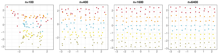
Figure 5: Latent position recovery in the sparse regime by spectral embedding followed by Isomap for increasing $n$ and increasing sparsity. To aid visualisation, all plots display a subset of $100$ estimated positions corresponding to true positions on a sub-grid which is common across $n$. Estimated positions are coloured according to their true $y$-coordinate.

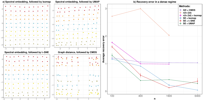
Figure 7: Latent position recovery in a dense regime. a) Recovery using different combinations of technique with $n=6400$. b) Average recovery error. The recovery error is an average over nodes and over 100 simulations, with two standard errors shown as vertical bars. Computational issues precluded showing node2vec for $n=6400$. (SE = spectral embedding, GD = graph distance and n2v = node2vec.)

B.2 Supplementary figures and discussion for flight network example

A gap appears to form between North and South America which, as a first hypothesis, we put down to the well-publicised suspension of all immigration into the US in April 2020. To measure this gap we use the Earth Mover’s distance between the point clouds belonging to the two continents (with thanks to Dr. Louis Gammelgaard Jensen for the code), using the approximate geodesic distances of the $\epsilon$-neighbourhood graph (i.e., before dimension reduction). While this distance does explode in April 2020, as shown in Figure 12 (Appendix), we found the proposed explanation to be incomplete, because Australia and New Zealand imposed similar measures at the time, whereas the distance between Oceania and the rest of the world, computed in the same way, does not explode. Revisiting the facts [2], while the countries mentioned above closed their borders to nonresidents, the continents of South America and Africa arguably imposed more severe measures, with large numbers of countries fully suspending flights. This explanation seems more likely, as on re-inspection we find a large jump in Earth mover’s distance, over April, between both of those continents and the rest of the world, as shown in Figure 13.

Figure 8: Visualisation of the global flight network over January 2020 by alternative combinations of techniques. The colours indicate continents (NA = North America, EU = Europe, AS = Asia, AF = Africa, OC = Oceania) and a spread of cities with high-traffic airports are labelled (to reduce clutter, only a selection of the cities in Figure 3 are shown).

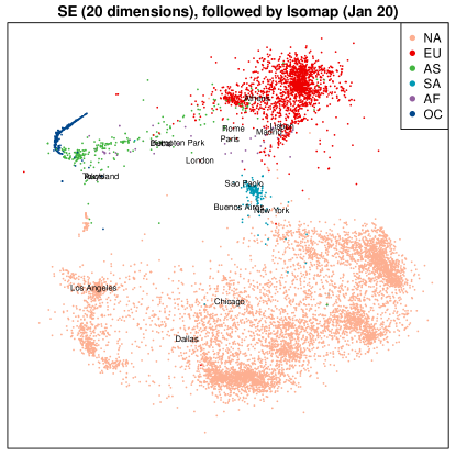
Figure 9: Visualisation of the global flight network. Spectral embedding into 20 dimensions followed by Isomap. The colours indicate continents (NA = North America, EU = Europe, AS = Asia, AF = Africa, OC = Oceania) and a spread of cities with high-traffic airports are labelled.

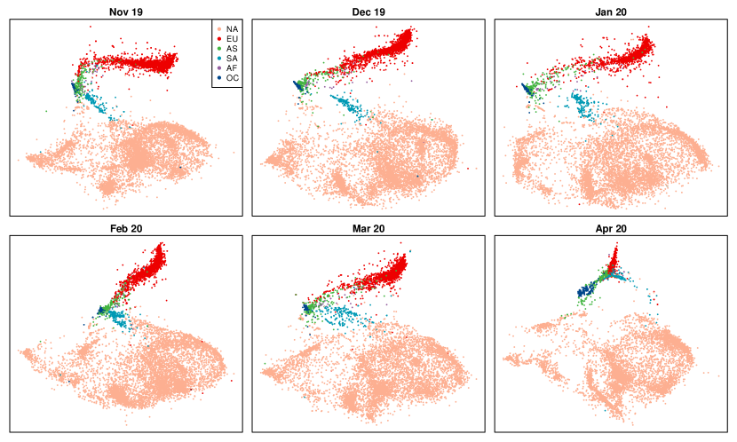
Figure 11: Visualisation of the global flight network over time: nonlinear dimension reduction of each spectral embedding using Isomap. The colours indicate continents (NA = North America, EU = Europe, AS = Asia, AF = Africa, OC = Oceania) and a spread of cities with high-traffic airports are labelled. An important structural change is observed in April 2020.

Figure 12: Earth mover’s distance between North and South America, as inferred from the approximate geodesic distances given by the $\epsilon$-neighbourhood graph. In each of 100 Monte Carlo iterations, the Earth Mover’s distance is computed based on 100 points randomly selected from each continent. We plot the average, with 2 standard errors in either direction indicated by the vertical bars.

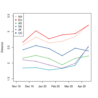
Figure 13: Earth mover’s distance from each continent to the rest of the world, as inferred from the approximate geodesic distances given by the $\epsilon$-neighbourhood graph. In each of 100 Monte Carlo iterations, the Earth mover’s distance is computed based on 100 points (airports) randomly selected from the continent of interest, and 100 points (airports) from the rest of the world. We plot the average, for each continent, with 2 standard errors in either direction indicated by the vertical bars.

B.3 Supplementary figures and discussion for temperature correlation example

Further to the discussion in Section 4, Figure 14 illustrates two important findings in the case $p=2$ and $d=1$, under the setup for this temperature correlation example described in section 4: firstly that there is no clear relationship between longitude and position along the manifold, and secondly a non-monotone relationship between longitude and estimated latent position. Both these observations are in marked contrast with the results in Figure 4 for latitude.

We then consider the case $p=3$ and $d=2$. Figure 15 shows the spectral embedding. Again the point-cloud is concentrated around a curved manifold. In Figure 16 we plot latitude and longitude against each of the $d=2$ coordinates of the estimated latent positions. As in the $p=2,d=1$ case, we find a clear monotone relationship between latitude and the first component of estimated position but no such relationship between longitude and the second component.

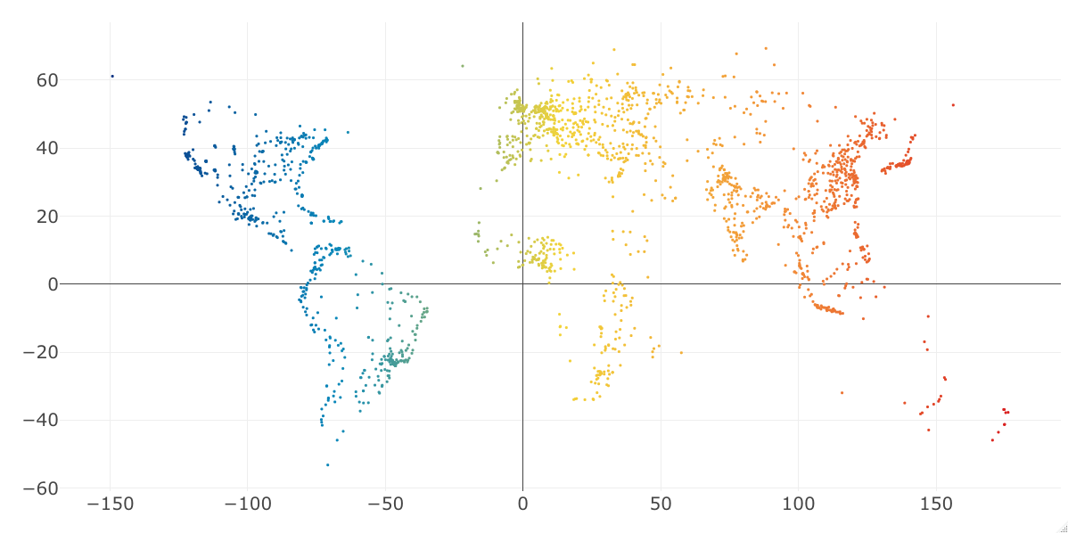
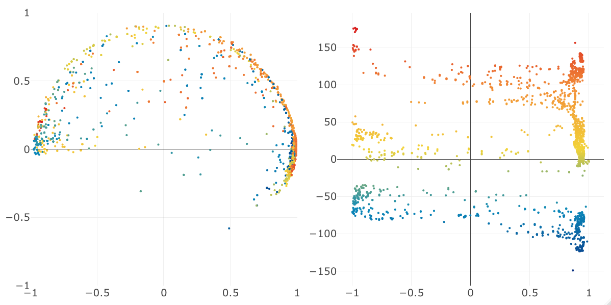
Figure 14: Temperature correlation example. Top: city locations. Bottom left: spectral embedding with $p=2$. Bottom right: true longitude (vertical axis) vs. estimated latent position (horizontal axis) with $d=1$. In all plots, points are coloured by longitudes of the corresponding cities.

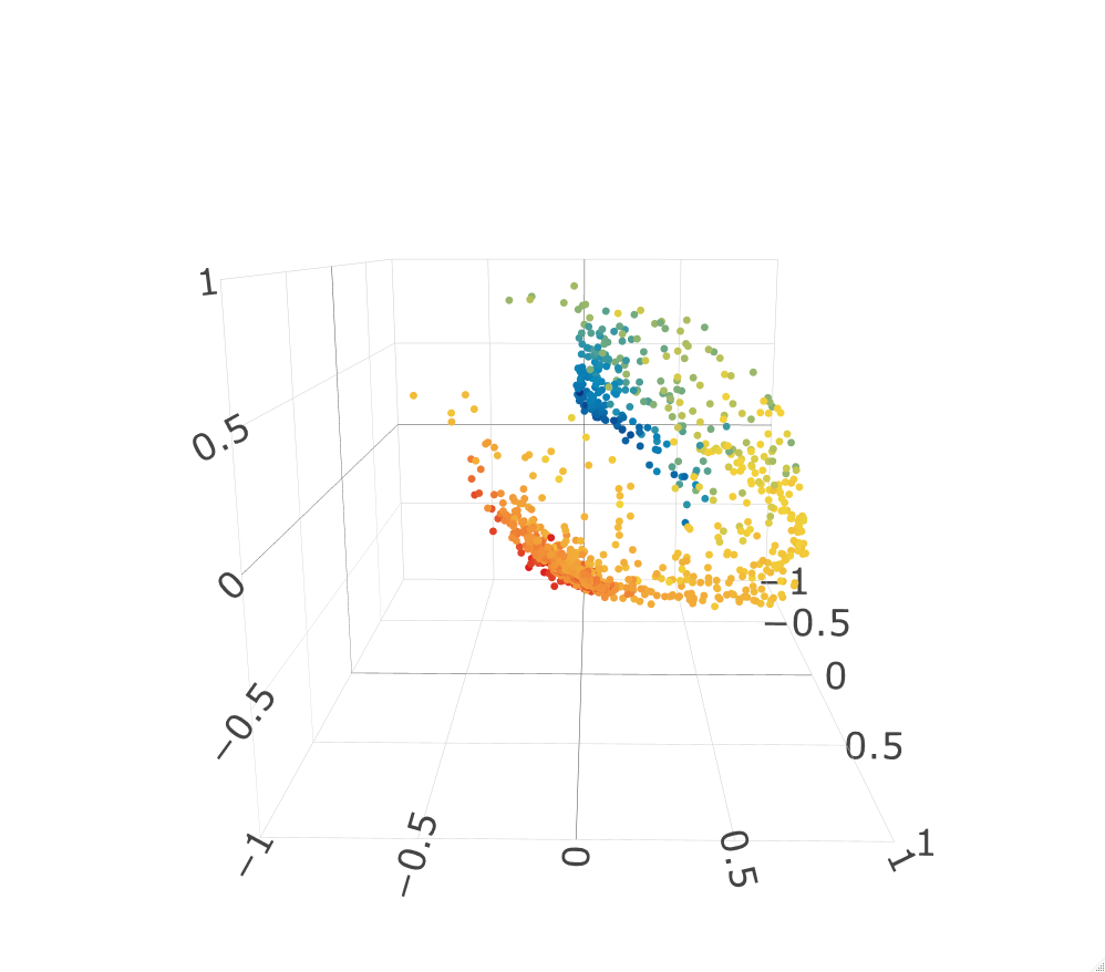
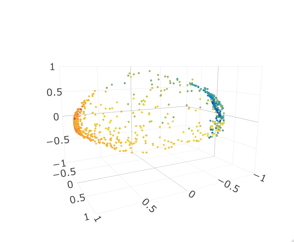
Figure 15: Temperature correlation example. Four views of the spectral embedding with $p=3$. In all plots, points are coloured by latitudes of the corresponding cities.

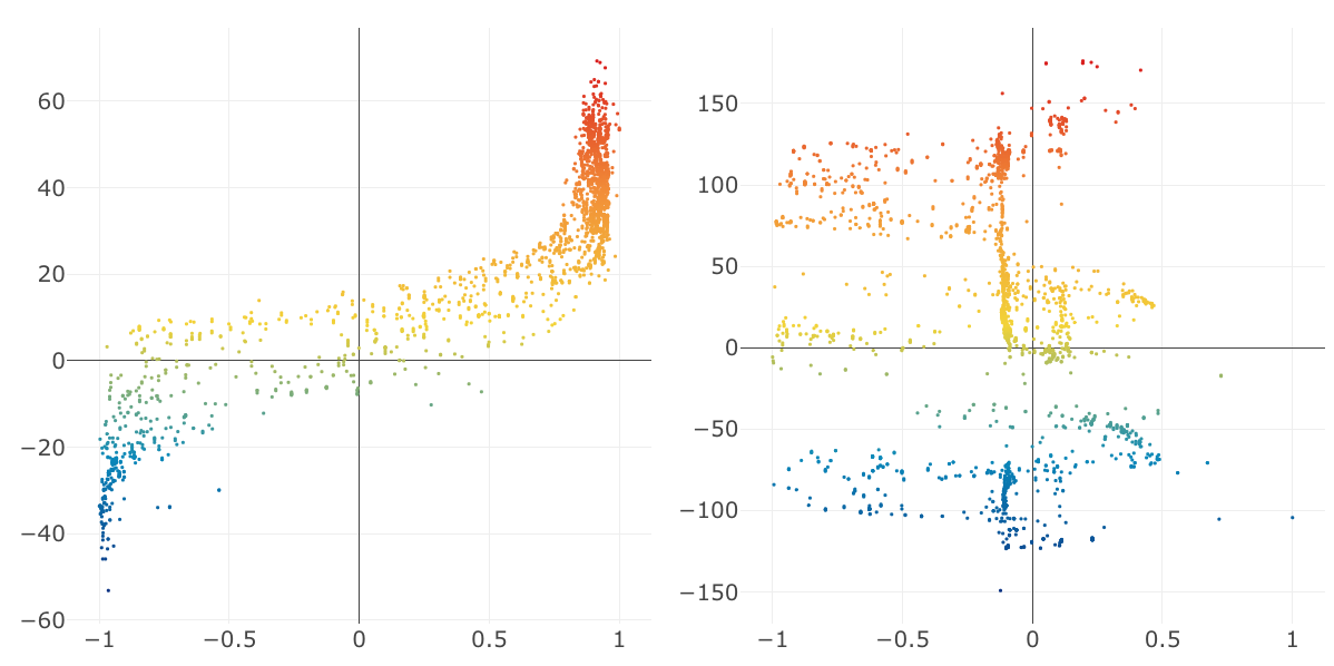
Figure 16: Temperature correlation example. Results for spectral embedding with $p=3$ followed by Isomap with $d=2$. Left: latitude (vertical axis) vs. estimated latent coordinate $\hat{Z}_{i}^{(1)}$ (horizontal axis) coloured by latitude. Right: longitude (vertical axis) vs. estimated latent coordinate $\hat{Z}_{i}^{(2)}$ (horizontal axis) coloured by longitude.

References

- [1] Berkeley Earth. http://berkeleyearth.org. Accessed: 2021-05-27.
- [2] Countries slammed their borders shut to stop coronavirus. but is it doing any good? https://www.npr.org/sections/goatsandsoda/2020/05/15/855669867/countries-slammed-their-borders-shut-to-stop-coronavirus-but-is-it-doing-any-goo. Accessed: 2021-05-20.
- [3] Climate change: Earth surface temperature data. https://www.kaggle.com/berkeleyearth/climate-change-earth-surface-temperature-data. Accessed: 2021-05-27.
- [4] Simplemaps free entire world database. https://simplemaps.com/resources/free-country-cities. Accessed: 2021-05-27.
- Abbe [2017] Emmanuel Abbe. Community detection and stochastic block models: recent developments. The Journal of Machine Learning Research, 18(1):6446–6531, 2017.
- Airoldi et al. [2008] Edoardo M Airoldi, David M Blei, Stephen E Fienberg, and Eric P Xing. Mixed membership stochastic blockmodels. Journal of Machine Learning Research, 9(Sep):1981–2014, 2008.
- Amari and Wu [1999] Shun-ichi Amari and Si Wu. Improving support vector machine classifiers by modifying kernel functions. Neural Networks, 12(6):783–789, 1999.
- Amini et al. [2013] Arash A Amini, Aiyou Chen, Peter J Bickel, and Elizaveta Levina. Pseudo-likelihood methods for community detection in large sparse networks. Annals of Statistics, 41(4):2097–2122, 2013.
- Anglade et al. [2019] Thomas Anglade, Christophe Denis, and Thierry Berthier. A novel embedding-based framework improving the User and Entity Behav- ior Analysis. working paper or preprint, October 2019. URL https://hal.sorbonne-universite.fr/hal-02316303.
- Araya Valdivia and Yohann [2019] Ernesto Araya Valdivia and De Castro Yohann. Latent distance estimation for random geometric graphs. In H. Wallach, H. Larochelle, A. Beygelzimer, F. d'Alché-Buc, E. Fox, and R. Garnett, editors, Advances in Neural Information Processing Systems, volume 32. Curran Associates, Inc., 2019. URL https://proceedings.neurips.cc/paper/2019/file/c4414e538a5475ec0244673b7f2f7dbb-Paper.pdf.
- Arias-Castro et al. [2021] Ery Arias-Castro, Antoine Channarond, Bruno Pelletier, and Nicolas Verzelen. On the estimation of latent distances using graph distances. Electronic Journal of Statistics, 15(1):722 – 747, 2021. doi: 10.1214/21-EJS1801. URL https://doi.org/10.1214/21-EJS1801.
- Athreya et al. [2017] Avanti Athreya, Donniell E Fishkind, Minh Tang, Carey E Priebe, Youngser Park, Joshua T Vogelstein, Keith Levin, Vince Lyzinski, and Yichen Qin. Statistical inference on random dot product graphs: a survey. The Journal of Machine Learning Research, 18(1):8393–8484, 2017.
- Athreya et al. [2021] Avanti Athreya, Minh Tang, Youngser Park, and Carey E Priebe. On estimation and inference in latent structure random graphs. Statistical Science, 36(1):68–88, 2021.
- Bickel et al. [2013] Peter Bickel, David Choi, Xiangyu Chang, and Hai Zhang. Asymptotic normality of maximum likelihood and its variational approximation for stochastic blockmodels. Annals of Statistics, 41(4):1922–1943, 2013.
- Bollobás et al. [2007] Béla Bollobás, Svante Janson, and Oliver Riordan. The phase transition in inhomogeneous random graphs. Random Structures & Algorithms, 31(1):3–122, 2007.
- Burago [2001] Dmitri Burago. A course in metric geometry, volume 33. American Mathematical Soc., 2001.
- Cape et al. [2019] Joshua Cape, Minh Tang, and Carey E Priebe. The two-to-infinity norm and singular subspace geometry with applications to high-dimensional statistics. The Annals of Statistics, 47(5):2405–2439, 2019.
- Gallagher et al. [2019] Ian Gallagher, Andrew Jones, Anna Bertiger, Carey Priebe, and Patrick Rubin-Delanchy. Spectral embedding of weighted graphs. arXiv preprint arXiv:1910.05534, 2019.
- Gao et al. [2015] Chao Gao, Yu Lu, and Harrison H Zhou. Rate-optimal graphon estimation. Annals of Statistics, 43(6):2624–2652, 2015.
- Grover and Leskovec [2016] Aditya Grover and Jure Leskovec. node2vec: Scalable feature learning for networks. In Proceedings of the 22nd ACM SIGKDD international conference on Knowledge discovery and data mining, pages 855–864, 2016.
- Hasan and Curry [2017] Souleiman Hasan and Edward Curry. Word re-embedding via manifold dimensionality retention. In Proceedings of the 2017 Conference on Empirical Methods in Natural Language Processing, pages 321–326, 2017.
- Hoff et al. [2002] Peter D Hoff, Adrian E Raftery, and Mark S Handcock. Latent space approaches to social network analysis. Journal of the American Statistical Association, 97(460):1090–1098, 2002.
- Holland et al. [1983] Paul W Holland, Kathryn Blackmond Laskey, and Samuel Leinhardt. Stochastic blockmodels: First steps. Social networks, 5(2):109–137, 1983.
- Janson and Olhede [2021] Svante Janson and Sofia Olhede. Can smooth graphons in several dimensions be represented by smooth graphons on ? arXiv preprint arXiv:2101.07587, 2021.
- Jones and Rubin-Delanchy [2020] Andrew Jones and Patrick Rubin-Delanchy. The multilayer random dot product graph. arXiv preprint arXiv:2007.10455, 2020.
- Kallenberg [1989] Olav Kallenberg. On the representation theorem for exchangeable arrays. Journal of Multivariate Analysis, 30(1):137–154, 1989.
- Kar and Karnick [2012] Purushottam Kar and Harish Karnick. Random feature maps for dot product kernels. In Artificial intelligence and statistics, pages 583–591. PMLR, 2012.
- Karam and Campbell [2010] Zahi N. Karam and William M. Campbell. Graph-embedding for speaker recognition. In Proc. Interspeech 2010, pages 2742–2745, 2010. doi: 10.21437/Interspeech.2010-726.
- Karrer and Newman [2011] Brian Karrer and Mark EJ Newman. Stochastic blockmodels and community structure in networks. Physical Review E, 83(1):016107, 2011.
- Lawrence and Hyvärinen [2005] Neil Lawrence and Aapo Hyvärinen. Probabilistic non-linear principal component analysis with Gaussian process latent variable models. Journal of machine learning research, 6(11), 2005.
- Lawrence [2003] Neil D Lawrence. Gaussian process latent variable models for visualisation of high dimensional data. In Nips, volume 2, page 5. Citeseer, 2003.
- Lei [2021] Jing Lei. Network representation using graph root distributions. The Annals of Statistics, 49(2):745–768, 2021.
- Lei and Rinaldo [2015] Jing Lei and Alessandro Rinaldo. Consistency of spectral clustering in stochastic block models. Ann. Statist., 43(1):215–237, 2015. ISSN 0090-5364. doi: 10.1214/14-AOS1274. URL https://doi.org/10.1214/14-AOS1274.
- Lovász [2012] László Lovász. Large networks and graph limits. American Mathematical Society Colloquium Publications, volume 60. Amer. Math. Soc. Providence, RI, 2012.
- Lyzinski et al. [2014] Vince Lyzinski, Daniel L. Sussman, Minh Tang, Avanti Athreya, and Carey E. Priebe. Perfect clustering for stochastic blockmodel graphs via adjacency spectral embedding. Electron. J. Stat., 8(2):2905–2922, 2014. doi: 10.1214/14-EJS978. URL https://doi.org/10.1214/14-EJS978.
- Lyzinski et al. [2017] Vince Lyzinski, Minh Tang, Avanti Athreya, Youngser Park, and Carey E Priebe. Community detection and classification in hierarchical stochastic blockmodels. IEEE Transactions on Network Science and Engineering, 4(1):13–26, 2017.
- Maaten and Hinton [2008] Laurens van der Maaten and Geoffrey Hinton. Visualizing data using t-SNE. Journal of machine learning research, 9(Nov):2579–2605, 2008.
- Margaryan et al. [2020] Ashot Margaryan, Daniel J Lawson, Martin Sikora, Fernando Racimo, Simon Rasmussen, Ida Moltke, Lara M Cassidy, Emil Jørsboe, Andrés Ingason, Mikkel W Pedersen, et al. Population genomics of the viking world. Nature, 585(7825):390–396, 2020.
- McInnes et al. [2018] Leland McInnes, John Healy, and James Melville. Umap: Uniform manifold approximation and projection for dimension reduction. arXiv preprint arXiv:1802.03426, 2018.
- Modell and Rubin-Delanchy [2021] Alexander Modell and Patrick Rubin-Delanchy. Spectral clustering under degree heterogeneity: a case for the random walk Laplacian. arXiv preprint arXiv:2105.00987, 2021.
- Petersen [2006] Peter Petersen. Riemannian geometry, volume 171 of Graduate Texts in Mathematics. Springer, 2006.
- Priebe et al. [2019] Carey E Priebe, Youngser Park, Joshua T Vogelstein, John M Conroy, Vince Lyzinski, Minh Tang, Avanti Athreya, Joshua Cape, and Eric Bridgeford. On a two-truths phenomenon in spectral graph clustering. Proceedings of the National Academy of Sciences, 116(13):5995–6000, 2019.
- Qiu et al. [2018] Jiezhong Qiu, Yuxiao Dong, Hao Ma, Jian Li, Kuansan Wang, and Jie Tang. Network embedding as matrix factorization: Unifying Deepwalk, LINE, PTE, and node2vec. In Proceedings of the eleventh ACM international conference on web search and data mining, pages 459–467, 2018.
- Rohe et al. [2011] Karl Rohe, Sourav Chatterjee, and Bin Yu. Spectral clustering and the high-dimensional stochastic blockmodel. Annals of Statistics, 39(4):1878–1915, 2011.
- Rubin-Delanchy [2020] Patrick Rubin-Delanchy. Manifold structure in graph embeddings. In Proceedings of the Thirty-fourth Conference on Neural Information Processing Systems, 2020.
- Rubin-Delanchy et al. [2020] Patrick Rubin-Delanchy, Joshua Cape, Minh Tang, and Carey E Priebe. A statistical interpretation of spectral embedding: the generalised random dot product graph. arXiv preprint arXiv:1709.05506, 2020.
- Rudin [1976] Walter Rudin. Principles of mathematical analysis, volume 3. McGraw-hill New York, 1976.
- Salter-Townshend and Murphy [2013] Michael Salter-Townshend and Thomas Brendan Murphy. Variational bayesian inference for the latent position cluster model for network data. Computational Statistics & Data Analysis, 57(1):661–671, 2013.
- Sanna Passino et al. [2020] Francesco Sanna Passino, Nicholas A Heard, and Patrick Rubin-Delanchy. Spectral clustering on spherical coordinates under the degree-corrected stochastic blockmodel. arXiv preprint arXiv:2011.04558, 2020.
- Schölkopf et al. [1998] Bernhard Schölkopf, Alexander Smola, and Klaus-Robert Müller. Nonlinear component analysis as a kernel eigenvalue problem. Neural computation, 10(5):1299–1319, 1998.
- Steinwart and Christmann [2008] Ingo Steinwart and Andreas Christmann. Support vector machines. Springer Science & Business Media, 2008.
- Strohmeier et al. [2021] Martin Strohmeier, Xavier Olive, Jannis Lübbe, Matthias Schäfer, and Vincent Lenders. Crowdsourced air traffic data from the opensky network 2019–2020. Earth System Science Data, 13(2):357–366, 2021.
- Sussman et al. [2012] Daniel L Sussman, Minh Tang, Donniell E Fishkind, and Carey E Priebe. A consistent adjacency spectral embedding for stochastic blockmodel graphs. Journal of the American Statistical Association, 107(499):1119–1128, 2012.
- Sutherland [2009] Wilson A Sutherland. Introduction to metric and topological spaces. Oxford University Press, 2009.
- Tang and Priebe [2018] Minh Tang and Carey E Priebe. Limit theorems for eigenvectors of the normalized laplacian for random graphs. The Annals of Statistics, 46(5):2360–2415, 2018.
- Tang et al. [2013] Minh Tang, Daniel L Sussman, and Carey E Priebe. Universally consistent vertex classification for latent positions graphs. The Annals of Statistics, 41(3):1406–1430, 2013.
- Tenenbaum et al. [2000] Joshua B Tenenbaum, Vin De Silva, and John C Langford. A global geometric framework for nonlinear dimensionality reduction. science, 290(5500):2319–2323, 2000.
- Tipping and Bishop [1999] Michael E Tipping and Christopher M Bishop. Probabilistic principal component analysis. Journal of the Royal Statistical Society: Series B (Statistical Methodology), 61(3):611–622, 1999.
- Titsias and Lawrence [2010] Michalis Titsias and Neil D Lawrence. Bayesian Gaussian process latent variable model. In Proceedings of the Thirteenth International Conference on Artificial Intelligence and Statistics, pages 844–851. JMLR Workshop and Conference Proceedings, 2010.
- Torgerson [1952] Warren S Torgerson. Multidimensional scaling: I. Theory and method. Psychometrika, 17(4):401–419, 1952.
- Trosset et al. [2020] Michael W Trosset, Mingyue Gao, Minh Tang, and Carey E Priebe. Learning 1-dimensional submanifolds for subsequent inference on random dot product graphs. arXiv preprint arXiv:2004.07348, 2020.
- Xu [2018] Jiaming Xu. Rates of convergence of spectral methods for graphon estimation. In International Conference on Machine Learning, pages 5433–5442. PMLR, 2018.
- Yamin et al. [2019] Abubakar Yamin, Michael Dayan, Letizia Squarcina, Paolo Brambilla, Vittorio Murino, V Diwadkar, and Diego Sona. Comparison of brain connectomes using geodesic distance on manifold: A twins study. In 2019 IEEE 16th International Symposium on Biomedical Imaging (ISBI 2019), pages 1797–1800. IEEE, 2019.
- Zhang and Tang [2021] Yichi Zhang and Minh Tang. Consistency of random-walk based network embedding algorithms. arXiv preprint arXiv:2101.07354, 2021.
- Zhu and Ghodsi [2006] Mu Zhu and Ali Ghodsi. Automatic dimensionality selection from the scree plot via the use of profile likelihood. Computational Statistics & Data Analysis, 51(2):918–930, 2006.