Assessing the Reliability of Deep Learning Classifiers Through Robustness Evaluation and Operational Profiles

Abstract

The utilisation of Deep Learning (DL) is advancing into increasingly more sophisticated applications. While it shows great potential to provide transformational capabilities, DL also raises new challenges regarding its reliability in critical functions. In this paper, we present a model-agnostic reliability assessment method for DL classifiers, based on evidence from robustness evaluation and the operational profile (OP) of a given application. We partition the input space into small cells and then “assemble” their robustness (to the ground truth) according to the OP, where estimators on the cells’ robustness and OPs are provided. Reliability estimates in terms of the probability of misclassification per input (pmi) can be derived together with confidence levels. A prototype tool is demonstrated with simplified case studies. Model assumptions and extension to real-world applications are also discussed. While our model easily uncovers the inherent difficulties of assessing the DL dependability (e.g. lack of data with ground truth and scalability issues), we provide preliminary/compromised solutions to advance in this research direction.

1 Introduction

Industry is adopting increasingly more advanced big data analysis methodologies to enhance the operational performance, safety, and lifespan of their products and services. For many products and systems high in-service reliability and safety are key targets to ensure customer satisfaction and regulatory compliance, respectively. AI and Deep Learning (DL) have steadily grown in interest and applications. Key industrial foresight reviews have identified that the biggest obstacle to reap the benefits of DL-powered robots is the assurance and regulation of their safety and reliability Lane et al. (2016). Thus, there is an urgent need to develop methods to enable the dependable use of AI/DL in critical applications Robu et al. (2018) and, more importantly, to assess and demonstrate the dependability for certification and regulation.

For traditional systems, safety and reliability analysis is guided by established standards, and supported by mature development processes and verification and validation (V&V) tools and techniques. The situation is different for systems that utilise DL: they require new and advanced analysis reflective of the complex requirements in their safe and reliable function. Such analysis also needs to be tailored to fully evaluate the inherent character of DL Bloomfield et al. (2019), despite the progress made recently Huang et al. (2020).

DL classifiers are subject to robustness concerns, reliability models without considering robustness evidence are not convincing. Reliability, as a user-centred property, depends on the end-users’ behaviours Littlewood and Strigini (2000). The operational profile (OP) information (quantifying how the software will be operated Musa (1993)) should therefore be explicitly modelled in the assessment. However, to the best of our knowledge, there is no dedicated reliability assessment model (RAM) taking into account both the OP and robustness evidence, which motivates this research.

In Zhao et al. (2020a), we propose a safety case framework tailored for DL, in which we describe an initial idea of combining robustness verification and operational testing for reliability claims. In this paper, we implement this idea as a RAM, inspired by partition-based testing Hamlet and Taylor (1990), operational-profile testing Strigini and Littlewood (1997); Zhao et al. (2020c) and DL robustness evaluation Carlini and Wagner (2017); Webb et al. (2019). It is model-agnostic and designed for pretrained DL models, yielding upper bounds on the probability of miss-classifications per input (pmi) with confidence levels. Although our RAM is theoretically sound, we discover some issues in our case studies (e.g. scalability and lack of data) that we believe represent the inherent difficulties of assessing/assuring DL dependability.

The key contributions of this work are:

a) A first RAM for DL classifiers based on the OP information and robustness evidence.

b) Discussions on model assumptions and extension to real-world applications, highlighting the inherent difficulties of assessing DL dependability uncovered by our model.

b) A prototype tool of our RAM with preliminary and compromised solutions to those uncovered difficulties.

Related Work

In recent years, there has been extensive efforts in verifying DL robustness, evaluating generalisation errors, and detecting adversarial examples (AEs). They are normally based on formal methods Huang et al. (2017); Katz et al. (2019) or statistical approaches Webb et al. (2019); Weng et al. (2019). A comprehensive review of those techniques can be sourced from recent survey papers Huang et al. (2020); Zhang et al. (2020). To the best of our knowledge, the only papers on testing DL for assessment within an operational context are Li et al. (2019); Guerriero et al. (2021). In Li et al. (2019), novel stratified sampling methods are used to improve the operational testing efficiency. Similarly, Guerriero et al. (2021) presents a sampling method from the operational dataset leveraging “auxiliary information for misclassification”, so that it provides unbiased statistical assessment while exposing as many misclassifications as possible. However, neither of them considers robustness evidence in their assessment models.

At the higher level of whole-systems utilising DL, although there are RAMs based on operational data, knowledge from low-level DL components is usually ignored, e.g., Kalra and Paddock (2016). In Zhao et al. (2020c), we improved Kalra and Paddock (2016) by providing a Bayesian mechanism to combine such knowledge, but did not show where to obtain the knowledge. In that sense, this paper is also a follow up of Zhao et al. (2020c), forming the prior knowledge required.

Organisation of the paper

We first present preliminaries on OP-based software reliability assessment and DL robustness. Then Section 3 describes the RAM in details with a running example. We conduct case studies in Section 3, while discuss the model assumptions and extensions in Section 5. Finally, we conclude in Section 6 with future work.

2 Preliminaries

2.1 OP Based Software Reliability Assessment

The delivered reliability, as a user-centred and probabilistic property, requires to model the end-users’ behaviours (in the running environments) and to be formally defined by a quantitative metric Littlewood and Strigini (2000). Without loss of generality, we focus on pmi as a generic metric for DL classifiers, where inputs are, e.g., facial images uploaded by users for facial recognition. We discuss later how pmi can be redefined to cope with real-world applications like traffic sign detection. If we denote the unknown pmi as a variable $\lambda$, then

$$\lambda:=\int_{x\in\mathcal{X}}I_{\{x\text{ causes a misclassification}\}}(x)Op(x)\mathop{}\!\mathrm{d}{x}$$ (1)

where $x$ is an input in the input domain $\mathcal{X}$, and ${I}_{\tt S}$ is an indicator function—it is equal to 1 when S is true and 0 otherwise. The $Op(x)$ returns the probability that $x$ is the next random input, the OP Musa (1993), a notion used in software engineering to quantify how the software will be operated. Mathematically, the OP is a probability density function (PDF) defined over $\mathcal{X}$.

Assuming independence between successive inputs defined in our pmi, we may use the Bernoulli process as the mathematical abstraction of the failure process (common for such “on-demand” type of systems), which implies a Binomial likelihood. Normally for traditional software, upon establishing the likelihood, RAMs on estimating $\lambda$ vary case by case—from the basic Maximum Likelihood Estimation (MLE) to Bayesian estimators tailored for certain scenarios when, e.g., seeing no failure Bishop et al. (2011), inferring ultra-high reliability Zhao et al. (2020c), with certain forms of prior knowledge like perfectioness Strigini and Povyakalo (2013), and with vague prior knowledge that expressed in imprecise probabilities Walter and Augustin (2009); Zhao et al. (2019).

OP based RAMs designed for traditional software fail to consider new characteristics of DL, e.g., unrobustness and high-dimensional input space. Specifically, it is quite hard to have the required prior knowledge in those Bayesian RAMs. While frequentist RAMs would require a large sample size to gain enough confidence in the estimates due to the extremely large population size (high-dimensional pixel space), especially for a high-reliable DL model where misclassifications are rare-events. As an example, the usual accuracy testing of DL classifiers is essentially an MLE estimate against the test set. It not only assumes the test set statistically represents the OP (our Assumption 3 later), but also requires a large number of samples to claim high reliability with sufficient confidence.

2.2 DL Robustness and the $R$-Separation Property

DL is known not to be robust. Robustness requires that the decision of the DL model ${\cal M}$ is invariant against small perturbations on inputs. That is, all inputs in a region $\eta\subset\mathcal{X}$ have the same prediction label, where usually the region $\eta$ is a small norm ball (in a $L_{p}$-norm distance) of radius $\epsilon$ around an input $x$. Inside $\eta$, if an input $x^{\prime}$ is classified differently to $x$ by ${\cal M}$, then $x^{\prime}$ is an AE. Robustness can be defined either as a binary metric (if there exists any adversarial example in $\eta$) or as a probabilistic metric (how likely the event of seeing an adversarial example in $\eta$ is). The former aligns with formal verification, e.g. Huang et al. (2017), while the latter is normally used in statistical approaches, e.g. Webb et al. (2019). The former “verification approach” is the binary version of the latter “stochastic approach”.

Similar to Webb et al. (2019), we adopt the more general probabilistic definition on the robustness of the model ${\cal M}$ (in a region $\eta$ and to a target label $y$):

$$R_{{\cal M}}(\eta,y):=\sum_{x\in\eta}I_{\{{\cal M}(x)\text{ predicts label }y\}}(x)\times Op(x\mid x\in\eta)$$ (2)

where $Op(x\mid x\in\eta)$ is the conditional OP of region $\eta$ (precisely the “input model” defined in Webb et al. (2019) and also used in Weng et al. (2019)).

We highlight the follow two remarks regarding robustness:

Remark 1 (astuteness).

Reliability assessment only concerns the robustness to the ground truth label, rather than an arbitrary label $y$ in $R_{{\cal M}}(\eta,y)$. When $y$ is such a ground truth, robustness becomes astuteness Yang et al. (2020), which is also the conditional reliability in the region $\eta$.

Astuteness is a special case of robustness. An extreme example showing why we introduce the concept of astuteness is: a perfectly robust classifier that always outs “dogs” for any given input is unreliable. Thus, robustness evidence cannot directly support reliability claims unless the ground truth label is used in $R_{{\cal M}}(\eta,y)$.

Remark 2 ($r$-separation).

For real-world image datasets, any data-points with different ground truth are at least distance $2r$ apart in the input space $\mathcal{X}$ (i.e., pixel space), and $r$ is bigger than usual norm ball radius in robustness studies.

The $r$-separation property was first observed by Yang et al. (2020): real-world image datasets studied by the authors implies that $r$ is normally $3\sim 7$ times bigger than the radius (denoted $\epsilon$) of norm balls commonly used in robustness studies. Intuitively it says that, although the classification boundary is highly non-linear, there is a minimum distance between two real-world objects of different classes (cf. Figure 1 for a conceptual illustration). Moreover, such minimum distance is bigger than the usual norm ball size in robustness studies.

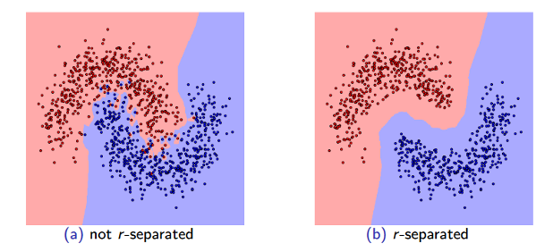
Figure 1: Illustration of the $r$-separation property.

3 A RAM for Deep Learning Classifiers

3.1 The Running Example

To better demonstrate our RAM, we take the Challenge of AI Dependability Assessment raised by the Siemens Mobility as a running example. Basically, the challenge is to firstly train a DL model to classify a dataset generated on the unit square $[0,1]^{2}$ according to some unknown distribution. The collected data-points (training set) are shown in Figure 2 (lhs). Then we need to build a RAM to claim an upper bound on the probability that the next random point is miss-classified, i.e. pmi. If the 2D-points represent traffic lights, then we have 2 types of misclassifications—safety-critical ones when red data-point is labelled green, and performance related otherwise. For brevity, we only focus on misclassifications here, while our RAM can cope with sub-types of misclassifications.

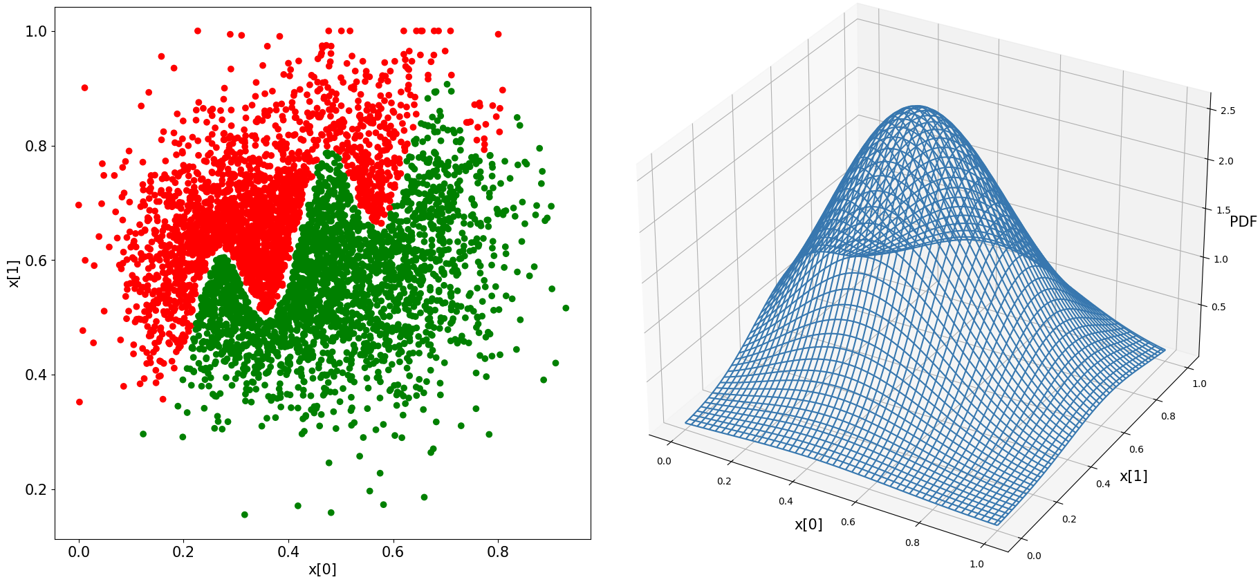
Figure 2: The 2D-point dataset (lhs), and its approximated OP (rhs).

3.2 The Model

The Framework

Inspired by Pietrantuono et al. (2020), the general idea of our RAM is to partition the input domain into $m$ small cells, subject to the $r$-separation property. Then, for each cell $c_{i}$ (with a single ground truth $y_{i}$), we estimate:

$$\lambda_{i} :=1-R_{{\cal M}}(c_{i},y_{i})\mbox{ and }Op_{i}:=\sum_{x\in c_{i}}Op(x)$$ (3)

which are the unastuteness and pooled OP, respectively, estimates of the cell $c_{i}$—we introduce estimators for both later. Then Eq. (1) can be written as the weighted sum of the cell-wise unastuteness (i.e. the conditional pmi of each cell) where the weights are the pooled OP of cells:

$$\lambda=\sum_{i=1}^{m}Op_{i}\lambda_{i}$$ (4)

Eq. (4) represents an ideal case in which we know those $\lambda_{i}$s and $Op_{i}$s with certainty. In practice, we can only estimate them with imperfect estimators yielding, e.g., a point estimate with variance capturing the measure of trust. To propagate the confidence in the estimates of $\lambda_{i}$s and $Op_{i}$s, we assume:

Assumption 1.

All $\lambda_{i}$s and $Op_{i}$s are independent unknown variables under estimations.

Then, the estimate of $\lambda$ and its variance are:

$${\mathbb{E}}[\lambda] =\sum_{i=1}^{m}{\mathbb{E}}[\lambda_{i}Op_{i}]=\sum_{i=1}^{m}{\mathbb{E}}[\lambda_{i}]{\mathbb{E}}[Op_{i}]$$ (5)

$${\mathbb{V}}[\lambda] =\sum_{i=1}^{m}{\mathbb{V}}[\lambda_{i}Op_{i}]$$

$$=\sum_{i=1}^{m}{\mathbb{E}}[\lambda_{i}]^{2}{\mathbb{V}}{[Op_{i}]}+{\mathbb{E}}[Op_{i}]^{2}{\mathbb{V}}[\lambda_{i}]+{\mathbb{V}}[\lambda_{i}]{\mathbb{V}}[Op_{i}]$$ (6)

Note that, for the variance, the covariance terms are dropped out due to the independence assumption.

Depending on the specific estimators adopted, certain parametric families of the distribution of $\lambda$ can be assumed, from which any quantile of interest (e.g. 95%) can be derived as our confidence bound in reliability. For instance, as readers will see later, we may assume $\lambda\sim\mathcal{N}({\mathbb{E}}[\lambda],{\mathbb{V}}[\lambda])$ since all $\lambda_{i}$s and $Op_{i}$s are normal distributed variables after applying the Central Limit Theorem (CLT) in our chosen estimators. Then, an upper bound with $1-\alpha$ confidence is

$$\mathit{Ub}_{1-\alpha}={\mathbb{E}}[\lambda]+z_{1-\alpha}\sqrt{{\mathbb{V}}[\lambda]}$$ (7)

where $Pr(Z\leq z_{1-\alpha})=1-\alpha$, and $Z\sim\mathcal{N}(0,1)$ is a standard normal distribution.

Now the the problem is reduced to how to obtain the estimates ${\mathbb{E}}[\lambda_{i}]$s and ${\mathbb{V}}[\lambda_{i}]$s, for which we will discuss as follows referring to the running example.

Partition of the Input Domain $\mathcal{X}$

As per Remark 1, the astuteness evaluation of a cell requires its ground truth label. To leverage the $r$-separation property and Assumption 4, we partition the input space by choosing a cell radius $\epsilon$ so that $\epsilon<r$. Although we concur with Remark 2 (first observed by Yang et al. (2020)) and believe that there should exist an $r$-stable ground truth (which means that the ground truth is stable in such a cell) for any real-world DL classification applications, it is hard to estimate such an $r$ (denoted by $\hat{r}$) and the best we can do is to assume:

Assumption 2.

There is a $r$-stable ground truth (as defined in Remark 2) for any real-world classification problems, and it can be sufficiently estimated from the existing dataset.

That said, we get $\hat{r}=0.004013$ by iteratively calculating the minimum distance of different labels in the running example. Then we choose a cell radius $\epsilon=0.004$ and partition the unit square $\mathcal{X}$ into $250\times 250$ cells.

Cell OP Approximation

Given a dataset $(X,Y)$, we estimate the pooled OP of cell $c_{i}$ to get ${\mathbb{E}}[Op_{i}]$ and ${\mathbb{V}}[Op_{i}]$. We use the well-established Kernel Density Estimation (KDE) to fit a $\widehat{Op}(x)$ to approximate the OP.

Assumption 3.

The existing dataset $(X,Y)$ are randomly sampled from the OP, thus statistically represents the OP.

This assumption may not hold in practice: training data is normally collected in a balanced way, since the DL model is expected to perform well in all categories of inputs, especially when the OP is unknown at the time of training and/or expected to change in future. Although our model can relax this assumption (cf. Section 5), we adopt it for brevity in demonstrating the running example.

Then given a set of (unlabelled) data-points $(X_{1},\dots,X_{n})$ from the existing dataset $(X,Y)$, KDE yields

$$\widehat{Op}(x)=\frac{1}{nh}\sum_{j=1}^{n}K(\frac{x-X_{j}}{h})$$ (8)

where $K$ is the kernel function (e.g. Gaussian or exponential kernels), and $h>0$ is a smoothing parameter called the bandwidth, cf. Silverman (1986) for guidelines on tuning $h$. The approximated OP is shown in Figure 2 (rhs).

Since our cells are small and all equal size, instead of calculating $\int_{x\in c_{i}}\widehat{Op}(x)dx$, we may approximate $Op_{i}$ as

$$\widehat{Op}_{i}=\widehat{Op}\left(x_{c_{i}}\right)v_{c}$$ (9)

where $\widehat{Op}(x_{c_{i}})$ is the probability density at the cell’s central point $x_{c_{i}}$, and $v_{c}$ is the constant cell volume ($1.6e{-5}$ in the running example).

Now if we introduce new variables $W_{j}=\frac{1}{h}K(\frac{x-X_{j}}{h})$, the KDE evaluated at $x$ is actually the sample mean of $W_{1},\dots,W_{n}$. Then by CLT, we have $\widehat{Op}(x)\sim\mathcal{N}(\mu_{W},\frac{\sigma_{W}^{2}}{n})$ where the mean and variance of $\widehat{Op}(x)$ are known results:

$${\mathbb{E}}[\widehat{Op}(x)] =\frac{1}{nh}\sum_{j=1}^{n}K(\frac{x-X_{j}}{h})$$ (10)

$${\mathbb{V}}[\widehat{Op}(x)] =\frac{f(x)\int K^{2}(u)du}{nh}+O(\frac{1}{nh})\approx\hat{\sigma}^{2}_{B}(x)$$ (11)

where the last step of Eq. (11) says that ${\mathbb{V}}[\widehat{Op}(x)]$ can be approximated using a bootstrap variance $\hat{\sigma}^{2}_{B}(x)$ Chen (2017) (cf. the Appendix A for details).

Upon establishing Eq.s (10) and (11), together with Eq. (9), we know for a given cell $c_{i}$ (knowing its central point $x_{c_{i}}$):

$${\mathbb{E}}[Op_{i}]=v_{c}{\mathbb{E}}[\widehat{Op}(x_{c_{i}})],\quad{\mathbb{V}}[Op_{i}]=v_{c}^{2}{\mathbb{V}}[\widehat{Op}(x_{c_{i}})]$$ (12)

which are the cell OP estimates for Eq.s (5) and (6).

Cell Astuteness Evaluation

As a corollary of Remark 2 and Assumption 2, we may confidently assume:

Assumption 4.

If the radius of $c_{i}$ is smaller than $r$, all data-points in the region $c_{i}$ share a single ground truth label.

Now, to determine the ground truth label of a cell $c_{i}$, we can classify our cells into three types:

a) Normal cells: a normal cell contains data-points sharing a same ground truth label, which is then determined as the ground truth label of the cell.

b) Empty cells: a cell is “empty” in the sense that no data-point that has been observed in it. Due to the lack of data, it is hard to determine an empty cell’s ground truth. For now, we do voting based on the predicted labels (by the DL model) of random samples from the cell, assuming:

Assumption 5.

The accuracy of the DL model is better than a classifier doing random classifications in any given cell.

Essentially the above assumption relates to the oracle problem of DL testing, that we see some recent efforts, e.g. Guerriero (2020), may relax it.

c) Cross-boundary cells: our estimate on $r$ is imperfect, thus we may still observe data-points with different labels in one cell. Such cells are crossing the classification boundary. If our estimate on $r$ is sufficiently accurate, they should be very rare. Thus, without the need to determine the ground truth label of a cross boundary cell, we simply and conservatively set the cell unastuteness to 1.

So far, the problem is reduced to: given a normal or empty cell $c_{i}$ with the known ground truth label $y_{i}$, evaluate the miss-classification probability upon a random input $x\in c_{i}$, i.e. ${\mathbb{E}}[{\lambda_{i}}]$ and its variance ${\mathbb{V}}[{\lambda_{i}}]$. This is essentially a statistical problem that has been studied in Webb et al. (2019) using Multilevel Splitting Sampling, while we use the Simple Monte Carlo method for brevity in the running example:

$$\hat{\lambda}_{i}=\frac{1}{n}\sum_{j=1}^{n}I_{\{M(x_{j})\neq y_{i}\}}$$

The CLT tells us $\hat{\lambda}_{i}\sim\mathcal{N}(\mu,\frac{\sigma^{2}}{n})$, when $n$ is large, where $\mu$ and $\sigma^{2}$ are population mean and variance of $I_{\{{\cal M}(x_{j})\neq y_{i}\}}$ that can be approximated with sample mean $\hat{\mu}_{n}$ and sample variance $\hat{\sigma}_{n}^{2}/n$. Finally, we can get

$${\mathbb{E}}[{\lambda_{i}}] =\hat{\mu}_{n}=\frac{1}{n}\sum_{j=1}^{n}I_{\{{\cal M}(x_{j})\neq y_{i}\}}$$ (13)

$${\mathbb{V}}[{\lambda_{i}}] =\frac{\hat{\sigma}_{n}^{2}}{n}=\frac{1}{(n-1)n}\sum_{j=1}^{n}(I_{\{{\cal M}(x_{j})\neq y_{i}\}}-\hat{\mu}_{n})^{2}$$ (14)

Notably, to solve the above statistical problem with sampling methods, we need to assume how the inputs in the cell are distributed, i.e., a distribution for the conditional OP $Op(x\mid x\in c_{i})$. Without loss of generality, we assume:

Assumption 6.

The inputs in a small region like cells are uniformly distributed.

which is not uncommon (e.g., in Webb et al. (2019); Weng et al. (2019)) and can be easily replaced by other distributions if there is supporting evidence for such action.

4 Case Studies

In addition to the running example, we conduct experiments on two synthetic datasets as shown in Figure 3, representing the scenarios with sparse and dense training data respectively. All modelling details and results after applying our RAM on those three datasets are summarised in Table 1, based on which we compare the testing error, Average Cell Unastuteness (ACU) and our RAM results (${\mathbb{E}}[\lambda]$ and $Ub_{97.5\%}$).

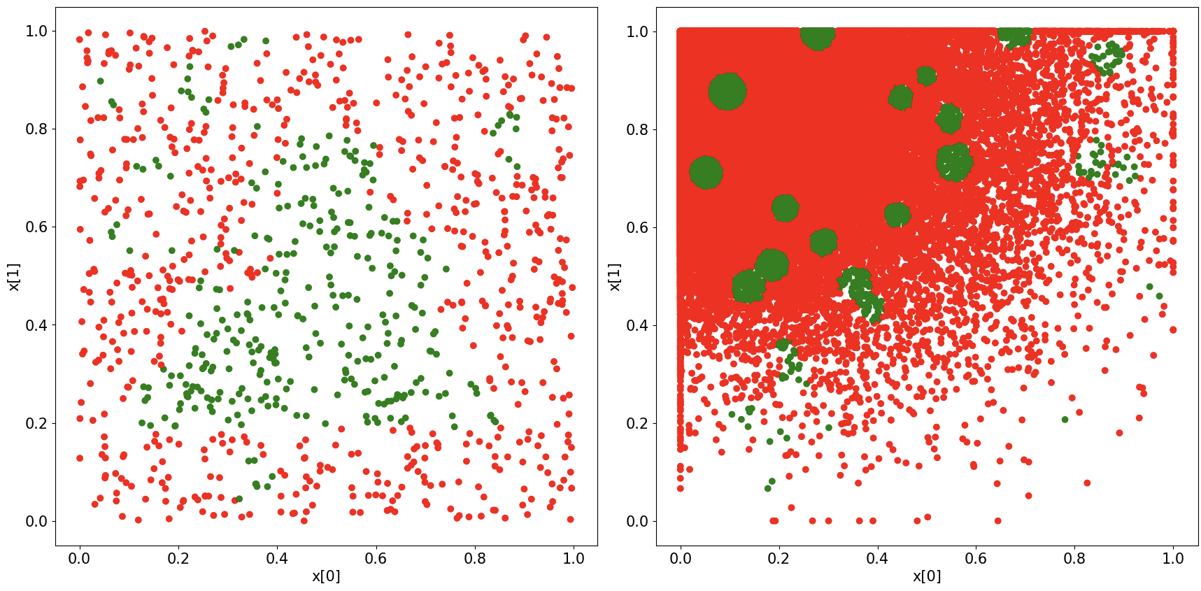
Figure 3: Synthetic datasets DS-1 (lhs) and DS-2 (rhs) representing relatively sparse and dense training data respectively.

Table 1: The RAM details and results. For image datasets, the $r$, $\epsilon$ and $\#$ are associated with latent spaces. Time is in seconds per cell.

	train/test error	$r$-separation	cell radius $\epsilon$	# of cells	ACU	${\mathbb{E}}[\lambda]$	${\mathbb{V}}[\lambda]$	$Ub_{97.5\%}$	time
The run. exp.	0.0005/0.0180	0.004013	0.004	$250\times 250$	0.002982	0.004891	0.000004	0.004899	0.04
Synth. DS-1	0.0037/0.0800	0.004392	0.004	$250\times 250$	0.008025	0.008290	0.000014	0.008319	0.03
Synth. DS-2	0.0004/0.0079	0.002001	0.002	$500\times 500$	0.004739	0.005249	0.000002	0.005252	0.04
MNIST	0.0051/0.0235	0.1003	0.100	top-170000	0.106615	0.036517	/	/	0.43
CIFAR10	0.0199/0.0853	0.1947	0.125	top-23000	0.238138	0.234419	/	/	6.74

In the running example, we first observe that the ACU is much lower than the test error, meaning the underlying DL model is a robust one. Since our RAM is mainly based on the robustness evidence, its results are close to ACU but not exactly the same because of the nonuniform OP, cf. Figure 2 (rhs). Moreover, from Figure 2 (lhs), we know the classification boundary is near the middle of the unit square input space where misclassifications tend to happen (say “buggy area”), which is also the high density area on the OP. Thus, the contribution to unreliability from the “buggy area” is weighted higher by the OP, which explains why our RAM results are worse than ACU. In contrast, because of the “flat” OP in the DS-1 (cf. Figure 3 (lhs)), our RAM results are very close to the ACU. With more dense data in DS-2, the $r$-distance is much smaller and leads to more cells. Thanks to the rich data in this case, all three results are more consistent. We note that, given the nature of the three 2D-point datasets, DL models trained on them are much more robust than image datasets. This is why all ACUs are better than test errors, and our RAM finds a middle point representing reliability according to the OP. Later we apply the RAM on two unrobust DL models trained on image-datasets where the ACUs are worse than test error; it confirms our aforementioned observations.

To gain insights on how to extend our method for high-dimensional/real-world datasets, we also conduct experiments on the popular MNIST and CIFAR10 datasets. Instead of implementing the exact steps in Section 3.2, we take a few compromised solutions to tackle the scalability issues raised by “the curse of dimensionality”. We articulate these steps in the following paragraph, while detailed discussions on their impact on our results are presented in Section 5.

First, we train Variational Auto-Encoders (VAE) on the MNIST and CIFAR10 datasets and project all inputs into the low dimensional latent spaces of VAE (with 8 and 16 dimensions respectively). Then we apply the proposed RAM on the compressed dataset, i.e., partitioning the latent space, learning the OP in latent space and evaluating the “latent-cell unastuteness”. Astuteness (a special case of robustness), by definition is associated with the input pixel space. By “latent-cell unastuteness”, we mean the average unastuteness of norm balls (in the input space) around a large number of samples from a “latent-cell”. The norm ball radius is determined by the $r$-separation distance in the input space. Taking the computational cost into consideration, we rank the OP of all latent-cells, and choose the top $k$ cells with highest OP for astuteness evaluation. We adopt the existing robustness estimator in Webb et al. (2019), where the authors omitted the result of ${\mathbb{V}}[\lambda_{i}]$; we therefore also omit the variance in our experiments for simplicity.

5 Discussions

In this section, we summarise the model assumptions made in our RAM, and discuss if/how they can be validated and what new-assumptions/compromised-solutions are needed to cope with high-dimensional/real-world applications. Finally, we list the inherent difficulties of assessing DL uncovered by our RAM.

Independent $\lambda_{i}$s and $Op_{i}$s

As per Assumption 1, we assume all $\lambda_{i}$s and $Op_{i}$s are independent when “assembling” their estimates via Eq. (5) and deriving the variance via Eq. (6). Largely this assumption is for the mathematical tractability when propagating the confidence in individual estimates at the cell-level to the whole system pmi. Although this independence assumption is hard to justify in practice, it is not unusual in reliability models that use partition, e.g. in Pietrantuono et al. (2020); Miller et al. (1992). We believe that RAMs are still useful as a first approximation under this assumption, while we envisage that Bayesian estimators leveraging joint priors and conjugacy may relax it.

$R$-separation and its estimation

Assumption 2 derives from Remark 2. We concur with Yang et al. (2020) and believe that, for any real-world DL classification applications where the inputs are data-points with “physical meanings”, there should always exist an $r$-stable ground truth. Such $r$ varies between applications, and the smaller the $r$ is, the harder the inherent difficulty of the classification problem is; i.e., $r$ is a difficulty indicator for the given classification problem.

For real-world applications, what really determines the label of an image are its features rather than pixels. Thus, we envisage some latent space (of, e.g., VAE) capturing only the feature-wise information can be explored for high-dimensional data. That is, we

• first do $r$-separation based partition in the latent space to learn the OP;

• then determine the ground truth labels of cells in the latent space;

• map the learned OP and ground truth labels back to the input pixel space;

• do astuteness evaluation in the input pixel space and “assemble” the results according to the OP.

Indeed, it is hard to estimate the $r$ (neither in the input nor the latent space), while the best we can do is to estimate it from the existing dataset. One way of solving the problem is to keep monitoring the $r$ estimates as more labelled data is collected, and redo the cell partition when the estimated $r$ has changed significantly.

Approximation of the OP

Assumption 3 says that the collected dataset statistically represents the OP, which may not hold for many practical reasons; e.g., the future OP is uncertain at the training stage and thus data is collected in a balanced way to perform well in all categories of inputs. Although we demonstrate our RAM under this assumption for simplicity, it can be easily relaxed. Essentially, we try to fit a density function over the input space from an “operational dataset” (representing the OP). Data-points in this set can be unlabelled raw data generated from historical data of previous applications, simulations and manually scaled based on expert knowledge. Obtaining such operational dataset is an application-specific engineering problem, and tractable thanks to the fact that it does not require labelled data.

Notably, the OP may also be approximated at runtime based on the data stream of operational data. Efficient KDE for data streams Qahtan et al. (2017) can be used. If the OP was subject to sudden changes, change-point detectors like Zhao et al. (2020b) should also be paired with the runtime estimator to robustly approximate the OP.

However, we may encounter technical challenges when fitting the PDF from high-dimensional real-world datasets. There are two known major challenges when applying multivariate KDE to high-dimensional data: i) the choice of bandwidth $H$ represents the covariance matrix that mostly impacts the estimation accuracy; ii) scalability issues in terms of storing intermediate data structure (e.g. data-points in hash-tables) and querying times made when estimating the density at a given input. For the first challenge, the optimal calculation of bandwidth matrix can refer to some rule of thumb Silverman (1986); Scott (2015) and the cross-validation Bergstra and Bengio (2012). While there are dedicated research on improving the efficiency of multivariate KDE, e.g., Backurs et al. (2019) presented a framework for multivariate KDE in provably sub-linear query time with linear space and linear pre-processing time to the dimensions.

Determination of the ground truth of a cell

Assumptions 4 and 5 are essentially on how to determine the ground truth label for a given cell, that relates to the oracle problem of testing DL Guerriero (2020). While it is still challenging, we partially solve it by leveraging the $r$-separation property.

Thanks to $r$, it is easy to determine a cell’s ground truth when we see it contains labelled data-points. However, for an empty cell, it is non-trivial. We assume the overall performance of the DL model is fairly good (e.g., better than a classifier doing random classifications), thus miss-classifications within an empty cell are relatively rare events. Then we can determine the ground truth label of the cell by majority voting of predictions. Indeed, this is a strong assumption when there are some “failure regions” in the input space that perform really badly (even worse than random labelling). In this case, we need to invent a new mechanism to detect such “really bad failure regions” and spend more budget on invoking, say, humans to do the labelling.

Conditional OP of a cell

We assume the distribution of inputs (i.e., the conditional OP) within each cell is uniform by Assumption 6. Although we conjecture that this is the common case due to the small size of cells (i.e., those very close/similar inputs within a small region are only subject to noise factors that can be modelled uniformly), the real situation may vary; this requires justification in safety cases.

For a real-world dataset, the conditional OP represents certain distributions of “natural variations” Zhong et al. (2021), e.g. lighting conditions, obey certain distributions. The conditional OP of cells should faithfully capture the distribution of such natural variations. Recent advance on measuring the natural/realistic AEs Harel-Canada et al. (2020) highly relates to this assumption and may relax it.

Explosion of the number of cells

The number of cells to evaluate the astuteness is exponential in the dimensions of data. For high-dimensional data, it is impossible to explore all cells in the input space as we did for the running example.

A compromised solution is to find the first $k$ cells that dominate the OP. That is, we rank the cells by their pooled OP, and only evaluate the top-$k$ cells where the sum of these $k$ cells’ OPs is greater than a threshold, e.g. 99%. Then, we can conservatively set the cell pmi of the rest to a worst-case bound (e.g. 1) or an empirical/average bound based on the first $k$ cells. Certainly, the price to pay is to sacrifice estimation accuracy. The best we can do for now is to increase the budgets for a larger $k$. Technically, finding the first $k$ cells dominating the OP is in fact to calculate the modes of the KDE function. The work of Lee et al. (2019) gives us a hint on how to quickly calculate the modes of Gaussian KDE when the data dimension is high.

This discussion relates to the cost of our RAM, thus a pertinent question is—what is the real cost of conducting DL testing? Is it the the human labour generating labels or timing constraints? A likely answer is: both. Our RAM has partially solved the former (cf. earlier discussions), while the latter is less costly nowadays and can be solved by harnessing the fast growth of computational power and parallel computing.

Efficiency of cell robustness evaluation

We have demonstrated via the Simple Monte Carlo method to evaluate cell robustness in the running example. It is well-known that Simple Monte Carlo is not a computationally efficient technique to estimate rare-events (such as AEs in our case) in high-dimensional space. Thus, instead of applying Simple Monte Carlo, the more advanced and efficient sampling approach, the Adaptive Multi-level Splitting method Webb et al. (2019), has been applied in our case studies on image datasets. We are confident that other statistical sampling methods designed for rare-events may also suffice our need.

In addition to the statistical approach, formal method based verification techniques can also be applied to assess a cell’s pmi, e.g. Huang et al. (2017). They provide formal guarantees on whether the DL model will miss-classify any input inside a small region. Although such “robust region” proved by formal methods is normally smaller than our cells, the $\hat{\lambda}_{i}$ can be conservatively set to the proportion of robust region covered in $c_{i}$ in this case.

We would like to note that the cell robustness estimator in our RAM works in a “hot-swappable” manner: any new and more efficient robustness estimator can be easily incorporated. Thus, how to improve the efficiency of cell’s robustness estimation is out of the scope of our RAM.

Inherent difficulties

Finally, based on our RAM and the discussions above, we summarise the inherent difficulties of assessing DL reliability as the following questions:

• How to accurately build the OP in the high-dimensional input space?

• How to build an accurate oracle leveraging the existing human-labels in the training dataset?

• What is the local distribution (conditional OP) over a small input region that captures the natural variations of physical conditions?

• How to efficiently evaluate the robustness of a small region given AEs are rare events?

• How to sample small regions from a large population (high-dimensional space) to test robustness in an unbiased and efficient way?

We try to provide preliminary/compromised solutions in our RAM, while the questions are still challenging in practice. We doubt the existence of other DL RAMs with weaker assumptions achieving the same level of rigorousness as ours, at this stage.

6 Conclusion & Future Work

In this paper, we present a preliminary RAM for DL classifiers. It is the first DL RAM explicitly considers both the OP information and robustness evidence. It uncovers some inherent difficult questions when assessing DL reliability, while preliminary/compromised solutions are discussed, implemented and demonstrated with case studies.

An intuitive way of perceiving our RAM, comparing with the usual accuracy testing, is that we enlarge the testing dataset with more test cases around “seeds” (original data-points in the test set). We determine the oracle of a new test case according to its seed’s label and the $r$-distance. Those enlarged test results form the robustness evidence, and how much they contribute to the overall reliability is proportional to its OP. Consequently, exposing to more tests (robustness evaluation) and being more representative of how it will be used (the OP), our RAM is more trustworthy.

In line with the gist of our RAM, we believe the DL reliability should follow the conceptualised equation of:

$$DL\,\,\,reliability=generalisability\times robustness.$$

In a nutshell, when assessing the DL reliability, we should not only concern how it generalises to a new data-point (according to the future OP), but also the local robustness around it. Align with this insight, indeed, a “naive/over-simplified” version of our RAM would be averaging all local astuteness of data-points in the test set, which is less rigorous (e.g., on determining the norm ball size) and requires stronger assumptions (e.g., the test set is equal to the operational set).

Improving the scalability of our RAM and experimenting with more real-world datasets form important future work. We presume a trained DL model for our assessment purpose. A natural question next is how to actually improve the reliability when our RAM results are not good enough. As described in Zhao et al. (2021), we plan to investigate DL debug testing (e.g. Huang et al. (2021)) and retraining methods Bai et al. (2021), together with the RAM, to form a closed loop of debugging-improving-assessing.

Appendix A KDE bootstrapping

Bootstrapping is a statistical approach to estimate any sampling distribution by random sampling method. We sample with replacement from the original data points $(X,Y)$ to obtain a new bootstrap dataset $(X^{b},Y^{b})$ and train the KDE on the bootstrap dataset. Assume the bootstrap process is repeated $B$ times, leading to $B$ bootstrap KDEs, denoted as $\widehat{Op}^{1}(x),\dots,\widehat{Op}^{B}(x)$. Then we can estimate the variance of $\hat{f}(x)$ by the sample variance of the bootstrap KDE Chen (2017):

$$\hat{\sigma}_{B}^{2}(x)=\frac{1}{B-1}\sum_{b=1}^{B}(\widehat{Op}^{b}(x)-\mu_{B})^{2}$$

where the $\mu_{B}$ can be approximated by

$$\hat{\mu}_{B}(x)=\frac{1}{B}\sum_{b=1}^{B}\widehat{Op}^{b}(x).$$

References

- Backurs et al. [2019] Arturs Backurs, Piotr Indyk, and Tal Wagner. Space and time efficient kernel density estimation in high dimensions. In NeurIPS’19, pages 15773–15782, 2019.
- Bai et al. [2021] Tao Bai, Jinqi Luo, Jun Zhao, Bihan Wen, and Qian Wang. Recent Advances in Adversarial Training for Adversarial Robustness. In IJCAI’21, 2021.
- Bergstra and Bengio [2012] James Bergstra and Yoshua Bengio. Random search for hyper-parameter optimization. J. of Machine Learning Research, 13(2):281–305, 2012.
- Bishop et al. [2011] Peter Bishop, Robin Bloomfield, Bev Littlewood, Andrey Povyakalo, and David Wright. Toward a formalism for conservative claims about the dependability of software-based systems. IEEE Transactions on Software Engineering, 37(5):708–717, 2011.
- Bloomfield et al. [2019] Robin Bloomfield, Heidy Khlaaf, Philippa Ryan Conmy, and Gareth Fletcher. Disruptive innovations and disruptive assurance: Assuring machine learning and autonomy. Computer, 52(9):82–89, 2019.
- Carlini and Wagner [2017] Nicholas Carlini and David Wagner. Towards Evaluating the Robustness of Neural Networks. In IEEE Symp. on Security and Privacy (SP), pages 39–57, San Jose, CA, USA, 2017. IEEE.
- Chen [2017] Yen-Chi Chen. A tutorial on kernel density estimation and recent advances. Biostatistics & Epidemiology, 1(1):161–187, 2017.
- Guerriero et al. [2021] Antonio Guerriero, Roberto Pietrantuono, and Stefano Russo. Operation is the hardest teacher: estimating DNN accuracy looking for mispredictions. In ICSE’21, Madrid, Spain, 2021.
- Guerriero [2020] Antonio Guerriero. Reliability Evaluation of ML systems, the oracle problem. In ISSREW’20, pages 127–130, Coimbra, Portugal, 2020. IEEE.
- Hamlet and Taylor [1990] D. Hamlet and R. Taylor. Partition testing does not inspire confidence. IEEE Tran. on Software Engineering, 16(12):1402–1411, 1990.
- Harel-Canada et al. [2020] Fabrice Harel-Canada, Lingxiao Wang, Muhammad Ali Gulzar, Quanquan Gu, and Miryung Kim. Is neuron coverage a meaningful measure for testing deep neural networks? In ESEC/FSE’20, pages 851–862, 2020.
- Huang et al. [2017] Xiaowei Huang, Marta Kwiatkowska, Sen Wang, and Min Wu. Safety verification of deep neural networks. In CAV’17, pages 3–29. Springer, 2017.
- Huang et al. [2020] Xiaowei Huang, Daniel Kroening, Wenjie Ruan, and et al. A survey of safety and trustworthiness of deep neural networks: Verification, testing, adversarial attack and defence, and interpretability. Computer Science Review, 37:100270, 2020.
- Huang et al. [2021] Wei Huang, Youcheng Sun, Xingyu Zhao, James Sharp, Wenjie Ruan, Jie Meng, and Xiaowei Huang. Coverage guided testing for recurrent neural networks. IEEE Tran. on Reliability, 2021. In press.
- Kalra and Paddock [2016] Nidhi Kalra and Susan M. Paddock. Driving to safety: How many miles of driving would it take to demonstrate autonomous vehicle reliability? Transportation Research Part A: Policy and Practice, 94:182 – 193, 2016.
- Katz et al. [2019] Guy Katz, Derek A. Huang, Duligur Ibeling, Kyle Julian, Christopher Lazarus, Rachel Lim, Parth Shah, Shantanu Thakoor, Haoze Wu, Aleksandar Zeljić, David L. Dill, Mykel J. Kochenderfer, and Clark Barrett. The Marabou Framework for Verification and Analysis of Deep Neural Networks. In CAV’19, volume 11561 of LNCS, pages 443–452, Cham, 2019. Springer.
- Lane et al. [2016] David Lane, David Bisset, Rob Buckingham, Geoff Pegman, and Tony Prescott. New foresight review on robotics and autonomous systems. Technical Report No. 2016.1, LRF, 2016.
- Lee et al. [2019] Jasper CH Lee, Jerry Li, Christopher Musco, Jeff M Phillips, and Wai Ming Tai. Finding the mode of a kernel density estimate. arXiv preprint arXiv:1912.07673, 2019.
- Li et al. [2019] Zenan Li, Xiaoxing Ma, Chang Xu, Chun Cao, Jingwei Xu, and Jian Lü. Boosting operational DNN testing efficiency through conditioning. In ESEC/FSE’19, pages 499–509. ACM, 2019.
- Littlewood and Strigini [2000] Bev Littlewood and Lorenzo Strigini. Software reliability and dependability: A roadmap. In ICSE 2000, pages 175–188, 2000.
- Miller et al. [1992] Keith W. Miller, Larry J. Morell, Robert E. Noonan, Stephen K. Park, David M. Nicol, Branson W. Murrill, and M Voas. Estimating the probability of failure when testing reveals no failures. IEEE Transactions on Software Engineering, 18(1):33–43, 1992.
- Musa [1993] John Musa. Operational profiles in software-reliability engineering. IEEE Software, 10(2):14–32, 1993.
- Pietrantuono et al. [2020] Roberto Pietrantuono, Peter Popov, and Stefano Russo. Reliability assessment of service-based software under operational profile uncertainty. Reliability Engineering & System Safety, 204:107193, 2020.
- Qahtan et al. [2017] Abdulhakim Qahtan, Suojin Wang, and Xiangliang Zhang. KDE-Track: An Efficient Dynamic Density Estimator for Data Streams. IEEE Transactions on Knowledge and Data Engineering, 29(3):642–655, 2017.
- Robu et al. [2018] Valentin Robu, David Flynn, and David Lane. Train robots to self-certify as safe. Nature, 553(7688):281–281, 2018.
- Scott [2015] David W Scott. Multivariate density estimation: theory, practice, and visualization. John Wiley & Sons, 2015.
- Silverman [1986] Bernard W Silverman. Density estimation for statistics and data analysis, volume 26. CRC press, 1986.
- Strigini and Littlewood [1997] Lorenzo Strigini and Bev Littlewood. Guidelines for statistical testing. Technical report, City, University of London, 1997.
- Strigini and Povyakalo [2013] Lorenzo Strigini and Andrey Povyakalo. Software fault-freeness and reliability predictions. In SafeComp’13, volume 8153 of LNCS, pages 106–117, Berlin, Heidelberg, 2013. Springer.
- Walter and Augustin [2009] Gero Walter and Thomas Augustin. Imprecision and prior-data conflict in generalized Bayesian inference. Journal of Statistical Theory & Practice, 3(1):255–271, 2009.
- Webb et al. [2019] Stefan Webb, Tom Rainforth, Yee Whye Teh, and M. Pawan Kumar. A statistical approach to assessing neural network robustness. In ICLR’19, New Orleans, LA, USA, 2019.
- Weng et al. [2019] Lily Weng, Pin-Yu Chen, Lam Nguyen, Mark Squillante, Akhilan Boopathy, Ivan Oseledets, and Luca Daniel. PROVEN: Verifying robustness of neural networks with a probabilistic approach. In ICML’19, volume 97, pages 6727–6736. PMLR, 2019.
- Yang et al. [2020] Yao-Yuan Yang, Cyrus Rashtchian, Hongyang Zhang, Ruslan Salakhutdinov, and Kamalika Chaudhuri. A Closer Look at Accuracy vs. Robustness. In NeurIPS’20, Vancouver, Canada, 2020.
- Zhang et al. [2020] J. M. Zhang, M. Harman, L. Ma, and Y. Liu. Machine learning testing: Survey, landscapes and horizons. IEEE Tran. on Software Engineering, 2020.
- Zhao et al. [2019] Xingyu Zhao, Valentin Robu, David Flynn, Fateme Dinmohammadi, Michael Fisher, and Matt Webster. Probabilistic model checking of robots deployed in extreme environments. In AAAI’19, volume 33, pages 8076–8084, 2019.
- Zhao et al. [2020a] Xingyu Zhao, Alec Banks, James Sharp, Valentin Robu, David Flynn, Michael Fisher, and Xiaowei Huang. A safety framework for critical systems utilising deep neural networks. In SafeComp’20, volume 12234 of LNCS, pages 244–259. Springer, 2020.
- Zhao et al. [2020b] Xingyu Zhao, Radu Calinescu, Simos Gerasimou, Valentin Robu, and David Flynn. Interval change-point detection for runtime probabilistic model checking. In ASE’20, pages 163–174. IEEE/ACM, 2020.
- Zhao et al. [2020c] Xingyu Zhao, Kizito Salako, Lorenzo Strigini, Valentin Robu, and David Flynn. Assessing safety-critical systems from operational testing: A study on autonomous vehicles. Information and Software Technology, 128:106393, 2020.
- Zhao et al. [2021] Xingyu Zhao, Wei Huang, Sven Schewe, Yi Dong, and Xiaowei Huang. Detecting operational adversarial examples for reliable deep learning. In 51th Annual IEEE-IFIP Int. Conf. on Dependable Systems and Networks (DSN’21), volume Fast Abstract, 2021.
- Zhong et al. [2021] Ziyuan Zhong, Yuchi Tian, and Baishakhi Ray. Understanding Local Robustness of Deep Neural Networks under Natural Variations. In FASE’21, pages 313–337, 2021.