TOI-674b: an oasis in the desert of exo-Neptunes transiting a nearby M dwarf

Abstract

Context. The NASA mission TESS is currently doing an all-sky survey from space to detect transiting planets around bright stars. As part of the validation process, the most promising planet candidates need to be confirmed and characterised using follow-up observations.

Aims. In this article we aim to confirm the planetary nature of the transiting planet candidate TOI-674b using spectroscopic and photometric observations.

Methods. We use TESS, Spitzer, ground-based light curves and HARPS spectrograph radial velocity measurements to establish the physical properties of the transiting exoplanet candidate TOI-674b. We perform a joint fit of the light curves and radial velocity time series to measure the mass, radius, and orbital parameters of the candidate.

Results. We confirm and characterize TOI-674b, a low-density super-Neptune transiting a nearby M dwarf. The host star (TIC 158588995, $V=14.2$ mag, $J=10.3$ mag) is characterized by its M2V spectral type with $\mathrm{M}_{\star}=0.420\pm 0.010$ M_⊙, $\mathrm{R}_{\star}=0.420\pm 0.013$ R_⊙, and $\mathrm{T}_{\mathrm{eff}}=3514\pm 57$ K, and is located at a distance $d=46.16\pm 0.03$ pc. Combining the available transit light curves plus radial velocity measurements and jointly fitting a circular orbit model, we find an orbital period of $1.977143\pm 3\times 10^{-6}$ days, a planetary radius of $5.25\pm 0.17$ $\mathrm{R}_{\oplus}$, and a mass of $23.6\pm 3.3$ $\mathrm{M}_{\oplus}$ implying a mean density of $\rho_{\mathrm{p}}=0.91\pm 0.15$ [g cm^-3]. A non-circular orbit model fit delivers similar planetary mass and radius values within the uncertainties. Given the measured planetary radius and mass, TOI-674b is one of the largest and most massive super-Neptune class planets discovered around an M type star to date. It is also a resident of the so-called Neptunian desert and a promising candidate for atmospheric characterisation using the James Webb Space Telescope.

1 Introduction

M dwarf stars are the most common type of stars in the Milky Way and in the solar neighborhood (e.g., Reid et al., 1995, Chabrier & Baraffe, 2000, Henry et al., 2006, Bochanski et al., 2010, Winters et al., 2015). Due to their relatively small sizes and low masses, they are good targets for the detection of small planets using transit searches and radial velocity measurements, respectively. More importantly, transiting planets orbiting bright M dwarfs offer great opportunities for atmospheric characterization using, for example, low and high resolution transmission spectroscopy (e.g., Kreidberg et al., 2014, Knutson et al., 2014, Ehrenreich et al., 2014, Southworth et al., 2017). Several Earth-sized and super-Earth planets have been found orbiting around M dwarfs (e.g., GJ 876d Rivera et al., 2005, TRAPPIST-1 system Gillon et al., 2017, LHS 1140b Dittmann et al., 2017, LHS 1140c Ment et al., 2019, GJ 357b Luque et al., 2019), but also planets with masses and radii between those of Neptune and Jupiter have been found (e.g., GJ 876c Marcy et al., 2001, GJ 436b Gillon et al., 2007; HATS-71b Bakos et al., 2020; GJ 3512b Morales et al., 2019; TOI-1728b Kanodia et al., 2020). Relatively few gas planets orbiting around M dwarfs have been found in this mass and size range, in agreement with the prediction of a paucity of gas giants orbiting around M dwarfs for core accretion models (Laughlin et al., 2004). Specifying their occurrence rate with better statistics can give new insights on planetary formation (e.g., core accretion versus disk instability: Boss, 2006) and orbital migration processes (e.g., Correia et al., 2020).

Planetary population studies made for different types of stars have noticed a lack of Neptune-sized planets with short orbital periods (i.e., highly irradiated), this is the so-called ‘Neptunian desert’ (e.g., Szabó & Kiss, 2011, Mazeh et al., 2016, Fulton & Petigura, 2018). The low number of Neptune-sized planets with orbital periods shorter than 4 days could possibly indicate different formation mechanisms for close-in super-Earths and Jovian planets (Mazeh et al., 2016), similar to what is observed for low-mass brown dwarfs in short orbits around Sun-like stars (e.g., Grether & Lineweaver, 2006). Another proposed mechanism for the origin of this gap in the radius distribution is photo-evaporation of planetary atmospheres in response to high energy radiation (ultraviolet, X-ray) from the star (e.g., Lopez & Fortney, 2013, Chen & Rogers, 2016).

In recent years, more planets in the Neptunian desert have been identified. Some examples of planets with masses close to Neptune and in short orbital periods found recently are NGTS-4b (West et al., 2019), TOI-132b (Díaz et al., 2020), LTT 9779b (Jenkins et al., 2020b), TOI-1728b (Kanodia et al., 2020), TOI-442b (Dreizler et al., 2020), TOI-849b (Armstrong et al., 2020). The addition of new objects in this mass, radius, and orbital period range can help to shed some light on the physical mechanisms behind the Neptunian desert.

The Transiting Exoplanet Survey Satellite (TESS; Ricker et al., 2014) is a NASA-sponsored space telescope launched in April 2018. Its main mission is to monitor the full sky in search of transiting planets orbiting around bright stars ($5<I_{C}<13$ mag). The observing strategy of TESS is to observe with its 4 cameras a $24^{\circ}\times 96^{\circ}$ area of the sky for 27 days. The exposure time for each camera is of 2 seconds and during the Primary Mission the images were stacked in two timing sampling modes: 2 minute and 30 minute cadence. The planned time for the main mission was 2 years, but on July 2020 TESS entered its extended mission which is approved to continue until the end of September 2022. For the first TESS extended mission the 30-minute cadence for Full Frame Images (FFIs) has been reduced to 10 minutes.

Here, we report the discovery of TOI-674b, a super-Neptune transiting around a nearby M dwarf, discovered using TESS data. The mass, radius, and orbital period of this planet indicate that this is a new member of the Neptunian desert, and it is a good candidate target for follow-up observations. This paper is organized as follows: Section 2 presents the observations used in this work, Section 3 presents the methods use in the data analysis, Section 4 presents the parameter estimates of the planet as well as a discussion in the context of known planets. Finally, Section 5 presents the conclusions of this work.

2 Observations

2.1 Space-based photometry

2.1.1 TESS photometry

The star TIC 158588995 (TOI-674) was observed by TESS during Sector 9 and Sector 10 for 27 days each. The Sector 9 campaign started on 28 February 2019 and ended on 25 March 2019; for this campaign the target was positioned on TESS CCD 3 Camera 2. The Sector 10 campaign started on 26 March 2019 and ended on 22 April 2019, and for this TESS run the target was placed on CCD 4 Camera 2. For its prime mission, TESS images were stacked in two timing sampling modes: 2 minute and 30 minute cadence; TOI-674 was selected to be observed using the 2 minute short-cadence mode in both sectors (Stassun et al., 2018b).

The raw image data taken by TESS was processed by the Science Processing Operations Center (SPOC) at NASA Ames Research Center. The SPOC pipeline (Jenkins et al., 2016) calibrates the image data, performs quality control (e.g., identifies and flags bad data), extracts photometry for each target star in the TESS field of view, and searches the resulting light curves for exoplanet transit signatures. The initial TESS light curve was produced using simple aperture photometry (SAP, Morris et al., 2020) and then the instrumental systematic effects were removed using the Presearch Data Conditioning (PDC) pipeline module (Smith et al., 2012, Stumpe et al., 2014). The light curves are searched with an adaptive, wavelet-based matched filter (Jenkins, 2002, Jenkins et al., 2020a) , and then fitted to limb-darkened transit models (Li et al., 2019) , and subjected to diagnostic tests to make or break the planetary hypothesis (Twicken et al., 2018). Subsequently, the TESS science office reviewed the transit signature identified in the SPOC processing of Sector 9, promoting it to a planetary candidate as TESS Object of Interest (TOI) TOI-674.01, and alerted the community in May 2019.

In this work we made used of the TESS PDC- SAP light curves that have been corrected for instrumental systematics. These data sets (TESS sector 9 and 10) are available at the Barbara A. Mikulski Archive for Space Telescopes (MAST). The TESS images around the position of TOI-674 in Sector 9 and 10 are shown in Figure 1. The red squares indicate the aperture used to produce the PDC-SAP light curves.

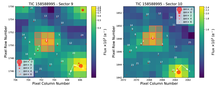
Figure 1: TESS target pixel file image of TOI 674 observed in Sector 9 (left) and Sector 10 (right), made with tpfplotter (Aller et al., 2020). The pixels highlighted in red show the aperture used as the target region in the photometry. The position and sizes of the red circles represent the position and TESS magnitudes of nearby stars respectively.

Table 1: TOI-674 identifiers, coordinates, stellar parameters, and magnitudes. The adopted stellar mass and radius used in this work are the ones presented in the middle column (i.e., BT-Settl models SED fit).

Identifiers					Ref.
TIC				158588995
2MASS				J10582099-3651292
Gaia EDR3				5400949450924312576
Equatorial coordinates
RA (J2016)				$10^{\mathrm{h}}\;58^{\mathrm{m}}\;20^{\mathrm{s}}.77$	1
DEC (J2016)				$-36^{\circ}\;51^{\prime}\;29\aas@@fstack{\prime\prime}19$	1
$\mu_{\alpha}$ [mas/year]				$-163.255\pm 0.015$	1
$\mu_{\delta}$ [mas/year]				$-3.672\pm 0.015$	1
Parallax [mas]				$21.623\pm 0.016$	1
Parameters from SED fit		BT-Settl SED fit		BT-Settl + Stellar evol. models SED fit
Effective Temperature [K]	$\mathrm{T}_{\mathrm{eff}}$	$3514\pm 57$		$3505^{+28}_{-32}$	5
Stellar Luminosity [$\mathrm{L}_{\odot}$]	$\mathrm{L}$	$0.0243^{+0.0012}_{-0.0009}$		$0.0240^{+0.0013}_{-0.0008}$	5
Surface gravity [cm/s2]	$\log(g)$	$5.28^{+0.51}_{-0.66}$		$4.832^{+0.006}_{-0.009}$	5
Metallicity [dex]	$[\mathrm{Fe}/\mathrm{H}]$	$0.17\pm 0.12$		$0.114\pm 0.074$	5
Stellar Age [Gyr]				$5.5^{+2.9}_{-1.9}$	5
Mass [M⊙]	$\mathrm{M}_{\star}$	$0.420\pm 0.010$		$0.442\pm 0.007$	5
Radius [R⊙]	$\mathrm{R}_{\star}$	$0.420\pm 0.013$		$0.421\pm 0.007$	5
Stellar density [g cm-3]	$\rho_{\star}$	$7.99\pm 0.76$		$8.36^{+0.22}_{-0.31}$	5
Surface gravity [cm/s2]	$\log(g)$	$4.81\pm 0.03$		$4.832^{+0.006}_{-0.009}$	5
Distance [pc]	$\mathrm{d}_{\star}$	$46.16\pm 0.03$		$46.16\pm 0.03$	5
Other parameters
Stellar activity index	$\log_{R_{HK}}$		$-5.14\pm 0.01$		5
Stellar rotation period [days]	$P_{\mathrm{rot}}$		$52\pm 5$		5
Stellar rotation velocity [km/s]			$0.4\pm 0.04$		5
Apparent magnitudes
Gaia G [mag]				$13.073\pm 0.002$	1
B [mag]				$15.742\pm 0.024$	2
V [mag]				$14.203\pm 0.041$	2
Sloan g [mag]				$14.938\pm 0.022$	2
Sloan r [mag]				$13.626\pm 0.047$	2
Sloan i [mag]				$12.299\pm 0.068$	2
J [mag]				$10.359\pm 0.023$	3
H [mag]				$9.737\pm 0.023$	3
K [mag]				$9.469\pm 0.019$	3
WISE W1 [mag]				$9.345\pm 0.022$	4
WISE W2 [mag]				$9.237\pm 0.019$	4
WISE W3 [mag]				$9.163\pm 0.038$	4
WISE W4 [mag]				$8.332\pm 0.455$	4

(1) Gaia Collaboration et al. (2021); (2) Henden et al. (2015); (3) Cutri et al. (2003); (4) Cutri & et al. (2014); (5) This work.

2.1.2 Spitzer photometry

A primary transit of TOI-674b was observed using the Spitzer Space Telescope as part of a program dedicated to TESS target follow-up (GO-14084, Crossfield et al., 2018). The data were taken with the instrument InfraRed Array Camera (IRAC), which is a four-channel camera with a field of view of $5.2^{\prime}\times 5.2^{\prime}$ and can take images at 3.6, 4.5, 5.8, and 8 $\mu$m. Each channel has $256\times 256$ pixels and a pixel scale of $\sim 1.2$ ″ pixel^-1. The target was observed on 29 September 2019 using Spitzer’s 4.5 $\mu$m channel, the exposure time was set to 2 seconds and the total observation time was $\sim 5$ hours. To compute the time series we used a $3\times 3$ pixel subarray centered on the position of TOI-674.

2.2 Ground-based photometry

After the discovery of the transits made by the TESS team, several follow-up ground-based observations were scheduled to confirm that the transits occur on TOI-674 and rule-out some false positive scenarios (e.g., eclipsing binaries unresolved by TESS). The data were acquired under the TESS Follow-up Observing Program (TFOP) and uploaded to the Exoplanet Follow-up Observing Program for TESS (ExoFOP-TESS).

2.2.1 El Sauce Observatory

We observed a full transit of TOI-674b in the Rc band on 12 May 2019 from El Sauce Observatory in Coquimbo Province, Chile. The 0.36 m telescope is equipped with a $1536\times 1024$ SBIG STT-1603-3 camera. The camera was operated using a $2\times 2$ bin mode, the image scale is 1.47 ″ pixel^-1 resulting in a $18.8\arcmin\times 12.5\arcmin$ field of view. The photometric data were extracted using AstroImageJ (Collins et al. 2017) with a 5 pixel aperture.

2.2.2 LCOGT

Las Cumbres Observatory Global Telescope Network (LCOGT, Brown et al., 2013) is a set of robotic telescopes operating in both hemispheres and with sites distributed across several countries. A primary transit of TOI-674b was observed on 16 May 2019 with the LCOGT 1 m telescope at Cerro Tololo International Observatory (CTIO) in Chile. The LCOGT 1 m telescopes are equipped with SINISTRO CCDs with a field of view of $26^{\prime}\times 26^{\prime}$ , and feature a pixel scale of 0.389 arcsec/pixel and read out cadence of 28 seconds. The transit was observed in the Sloan g band, the telescope was slightly defocused (0.1 mm from nominal value), and the exposure time was set to 150 seconds. The photometry was extracted using AstroImageJ software with an aperture of 10 pixels and the Point Spread Function (PSF) diameter was 1.95 arcsec.

2.2.3 TRAPPIST-South

TRAPPIST-South, located at ESO-La Silla Observatory in Chile, is a 60 cm Ritchey–Chretien telescope equipped with a thermoelectrically cooled $2K\times 2K$ FLI Proline CCD camera (Jehin et al., 2011; Gillon et al., 2013). It features a field- of-view of $22^{\prime}\times 22^{\prime}$ and a pixel-scale of 0.65 ″/pixel. We acquired 494 images during a full-transit observation on 2019-05-13 with the $I+z$ filter and an exposure time of 15 s. The optimum photometric aperture was 6 pixels (3.9 arcsec) and the PSF diameter 2.2 arcsec. A second full-transit observation was carried out on 2019-05-21 using the Sloan z filter with an exposure time of 15 s, and yielded a total of 412 images. The optimum aperture was 8 pixels (5.2 arcsec) and the PSF diameter was 2.5 arcsec. These sets of observations confirmed the presence of a transit event on the target star on time, and eliminated the possibility that the events are due to an eclipsing binary outside of the PSF centered on the target star. For both dates we made use of the TESS Transit Finder tool, which is a customized version of the Tapir software package (Jensen, 2013), to schedule the photometric time-series and we used AstroImageJ to perform aperture photometry.

2.3 Spectroscopic observations

TOI-674 was observed by the High Accuracy Radial velocity Planet Searcher (HARPS, Mayor et al., 2003) at the ESO La Silla 3.6m telescope. The observations were carried out as part of the program 1102.C-0339 dedicated to searching for planets orbiting around M dwarfs. From 24 May 2019 to 18 July 2019, we collected 17 spectra with a resolving power of $R\approx 115000$. The image of the target star was placed in the aperture of the scientific fiber while the calibration fiber was used to monitor the sky, the exposure time was set to 30 minutes and the CCD was read using the slow read-out mode, resulting in a signal-to-noise ratio between 5 and 13 (median of 9).

The spectra were calibrated and extracted using the HARPS online pipeline (Lovis & Pepe, 2007; for improvements in the pipeline check Mayor et al., 2009a, b and references therein). With the spectra and preliminary radial velocity measurements from the HARPS online pipeline we produced a template spectrum following Astudillo-Defru et al. (2017b). The final radial velocities were obtained from likelihood functions constructed by comparing the stellar template shifted by different velocities with each individual spectrum. The velocity that produced the maximum likelihood for each data point was the derived HARPS radial velocity. The RV time series present a dispersion of 17.4 m/s and have a median uncertainty of 7.3 m/s.

We also obtain from the spectra several activity indices: $\mathrm{H}_{\alpha}$, $\mathrm{H}_{\beta}$, $\mathrm{H}_{\gamma}$, Na, and calcium S index. The radial velocities and activity indices are given in Table 3.

2.4 High-resolution imaging

TESS has a pixel scale of 21 arcsec/pixel, hence it is possible that TOI-674 can present some level of flux contamination produced by nearby faint stars not detected by seeing limited photometric observations. Contamination in the flux of the transit host star can led to a wrong estimation of transit depth, thus leading to an incorrect absolute planet radius. TESS Data Validation Report (Twicken et al., 2018) performs a difference image centroiding analysis, in the case of TOI-674 the report determined that the location of the source of the transit signature was within 1 arcsec of the target star. Nevertheless, we searched for previously undetected faint nearby companion stars using adaptive optics and speckle imaging using Gemini Telescope.

2.4.1 Gemini/NIRI

We searched for visual companions with the Gemini/NIRI adaptive optics imager (Hodapp et al., 2003). Such companions can dilute the light curve, thereby biasing the measured radius, or even be the source of a false positive if the visual companion is an eclipsing binary (e.g., Ciardi et al., 2015). We collected 9 images in the Br$\gamma$ filter, each with exposure time 5.7 s, and dithered the telescope by $\sim$2” between each exposure. This dither pattern allows for a sky background frame to be constructed from the science images themselves. We processed the data using a custom code which performs bad pixel and flat corrections, subtracts the sky background, aligns the star between images and coadds the frames. The final image can be seen in Figure 2. We inspected the final image visually, and did not identify companions anywhere in the field of view, which is 26.8”$\times$26.8”. To estimate the sensitivity of these images to the presence of visual companions, we injected scaled copies of the stellar PSF at several radial separations and position angles, and scaled their brightness until each could be detected at 5-$\sigma$. Sensitivity was then averaged over position angle, and Figure 2 shows the sensitivity to visual companions as a function of radius. We are sensitive to companions 5 mag fainter than the host beyond 270 mas, and reach a contrast of 7.3 mag in the background limited regime, beyond $\sim$1.05”.

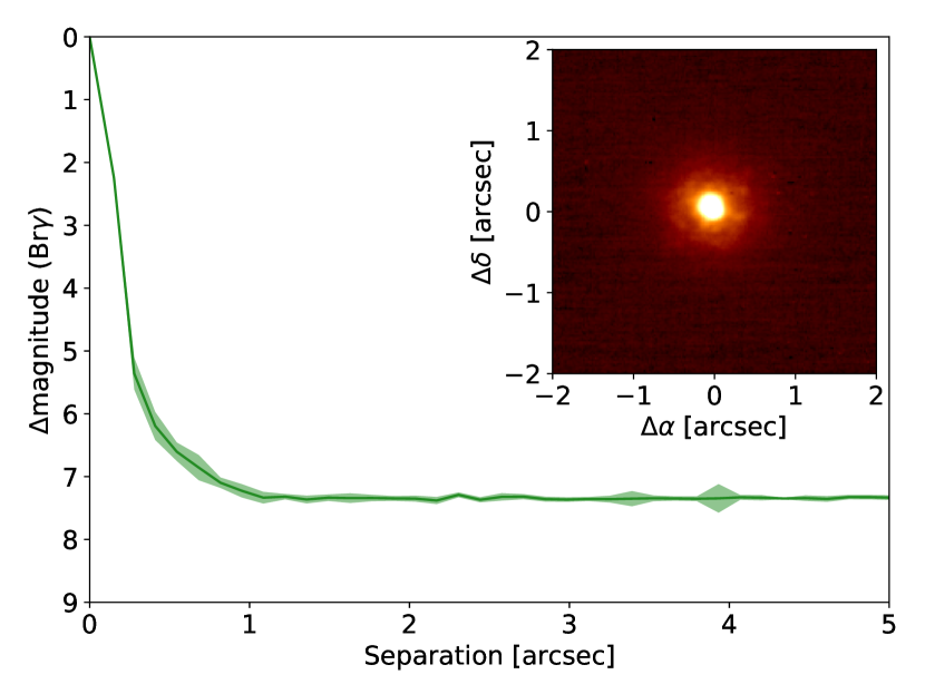
Figure 2: Gemini/NIRI high resolution image of TOI-674. Our observations rule out candidates to 5 mag fainter than the host beyond 270 mas, and 7.3 mag beyond $\sim$1.05″. Inset: thumbnail image of TOI-674, centered on the star. The PSF is circular to the limit of our resolution, and no visual companions are identified anywhere in the field of view, which extends at least 13″ from the target in all directions.

2.4.2 Gemini/Zorro

We observed TOI-674 on 14 January 2020 using the Zorro instrument mounted on the 8-m Gemini South telescope, located on Cerro Pachón in Chile. Zorro simultaneously observes diffraction-limited images at 562 nm (0.017”) and 832 nm (0.028”). Our data set consisted of five 1000 X 60 ms exposures simultaneously obtained in both band-passes, followed by a single $1000\times 60$ ms image, also in both band-passes, of a PSF standard star. Following the procedures outlined in Howell et al. (2011), we combined all images and subjected them to Fourier analysis, and produce re-constructed imagery from which 5-$\sigma$ contrast curves are derived in each passband (Figure 3). Our data reveal TOI-674 to be a single star to contrast limits of 5 to 7 magnitudes within the spatial limits of 0.8/1.3 AU (562/832 nm respectively) out to 55 AU ($\mathrm{d}=46$ pc). A second Gemini/Zorro observation made in 25 February 2021 confirmed the previous result and no companion stars to TOI-674 were detected within the angular and contrast limits explored.

Figure 3: Gemini/Zorro high resolution image of TOI-674 taken on 14 January 2020. TOI-674 is a single star to contrast limits of 5 to 7 mag within 0.8/1.3 AU (562/832 nm respectively) out to 55 AU ($\mathrm{d}=46$ pc). Inset: 1.2″x1.2″ thumbnail image of TOI-674, centered on the star.

3 Analysis

3.1 Stellar parameters

We computed an initial estimate of TOI-674 stellar parameters using the weighted average of the HARPS spectra and analysed it with SpecMatch-Emp (Yee et al., 2017). We thereby obtained $\mathrm{T_{eff}}=3470\pm 70$ K, $\mathrm{R_{\star}}=0.413\pm 0.100$ $\mathrm{R_{\odot}}$, and $[\mathrm{Fe}/\mathrm{H}]=0.18\pm 0.09$ dex. The parameters obtained with SpecMatch-Emp were used as a prior to fit the Spectral Energy Distribution (SED) of TOI-674. To estimate the stellar parameters we followed Díaz et al. (2014). For the SED fit we adopted the distance and the apparent magnitudes from Gaia (Gaia Collaboration et al., 2021), 2MASS (Cutri et al., 2003), and WISE (Cutri & et al., 2014). We used as priors the distance to the star (based on Gaia EDR3 parallax) and the effective temperature and value of $[\mathrm{Fe}/\mathrm{H}]$ from SpecMatch-Emp; the uncertainty in $[\mathrm{Fe}/\mathrm{H}]$ was changed from $0.09$ dex to $0.12$ dex according to Table 3 of Yee et al. (2017). The fit was done by comparing the SED with the synthetic spectra models from the BT-Settl library (Allard et al., 2011) alone and the BT-Settl library plus stellar evolution models from Dotter et al. (2008).

The stellar parameters for TOI-674 are presented in Table 1. The stellar mass value for the SED fit without stellar evolution models was computed following Mann et al. (2019) that uses the distance, K-magnitude, and metallicity to obtain a mass estimate. For the SED fit using BT-Settl stellar models we find a stellar effective temperature of $3514\pm 57$ K, indicating that the spectral type must be close to M2V. To be conservative in our uncertainties, we adopted as final stellar parameters the values found by the SED fit with stellar atmosphere models without including the stellar evolution models, i.e., middle column of Table 1. Hence, to derive absolute planet parameters we use in this work a stellar mass and radius of $\mathrm{M}_{\star}=0.420\pm 0.010$ M_⊙ and $\mathrm{R}_{\star}=0.420\pm 0.013$ R_⊙ respectively.

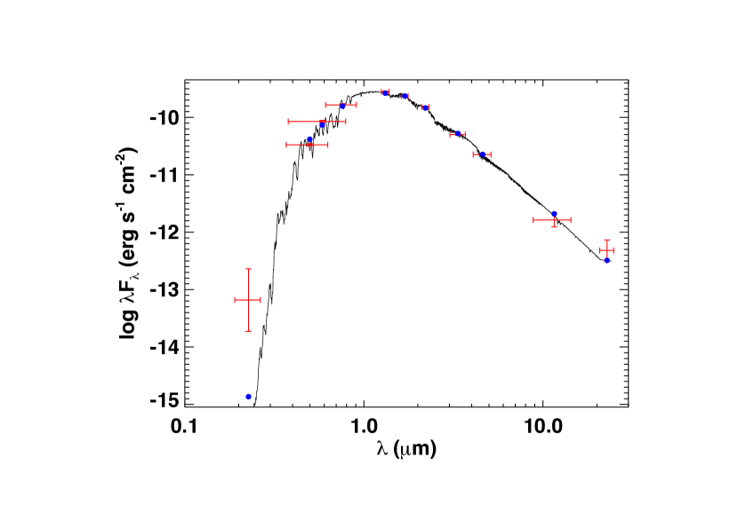
Figure 12: Spectral energy distribution of TOI-674. Red symbols represent the observed photometric measurements, where the horizontal bars represent the effective width of the passband. Blue symbols are the model fluxes from the best-fit NextGen atmosphere model (black).

To check our results and as an independent determination of the basic stellar parameters, we performed an analysis of the broadband spectral energy distribution (SED) of the star together with the Gaia EDR3 parallax (with no systematic correction Stassun & Torres, 2021), in order to determine an empirical measurement of the stellar radius, following the procedures described in Stassun & Torres (2016); Stassun et al. (2017, 2018a). We pulled the $JHK_{S}$ magnitudes from 2MASS, the W1–W4 magnitudes from WISE, the $GG_{\rm BP}G_{\rm RP}$ magnitudes from Gaia, and the NUV magnitude from GALEX. Together, the available photometry spans the full stellar SED over the wavelength range 0.2–22 $\mu$m (see Figure 12).

We performed a fit using NextGen stellar atmosphere models (Hauschildt et al., 1999), with the effective temperature ($T_{\rm eff}$), surface gravity ($\log g$), and metallicity ([Fe/H]) adopted from the spectroscopic analysis. The remaining free parameter is the extinction, $A_{V}$. The resulting fit (Figure 12) has a reduced $\chi^{2}$ of 3.1 (excluding the UV measurement which appears to be in excess, see below), with best fit $A_{V}=0.02\pm 0.02$. Integrating the (unreddened) model SED gives the bolometric flux at Earth, $F_{\rm bol}=3.50\pm 0.12\times 10^{-10}$ erg s^-1 cm^-2. Taking the $F_{\rm bol}$ and $T_{\rm eff}$ together with the Gaia parallax, gives the stellar radius, $R_{\star}=0.413\pm 0.015$ R_⊙; a value consistent with our adopted stellar radius presented in Table 1.

Finally, we can use the star’s activity to estimate an age via empirical rotation-activity-age relations. The mean chromospheric activity from the time-series spectroscopy is $\log R^{\prime}_{\rm HK}=-5.14\pm 0.01$, which implies a stellar rotation period of $P_{\rm rot}=52\pm 5$ days via the empirical relations of Astudillo-Defru et al. (2017a). This estimated $\mathrm{P}_{\rm rot}$ implies an age of $\tau_{\star}=3.2\pm 1.2$ Gyr via the empirical relations of Engle & Guinan (2018), which is consistent with the age derived from the SED fit plus stellar evolution models presented in Table 1.

3.2 Frequency analysis of the HARPS data

We searched for the planetary signal in the HARPS data using a generalized Lomb-Scargle periodogram (Zechmeister & Kürster, 2009). With the radial velocity measures alone a signal with a period of $\sim 2.0$ days is detected with a False Alarm Probability (FAP) below 1% ( $\mathrm{FAP}(peak)=0.15\%$, see Figure 4). This period is consistent with the orbital period originally reported by TESS team as part of their alerts ($P=1.977$ days).

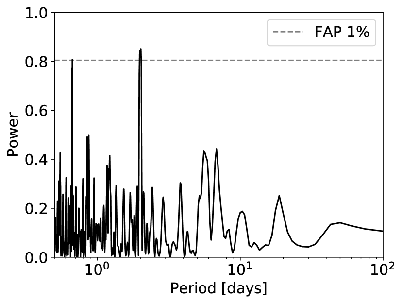
Figure 4: TOI-674b GLS periodogram for HARPS radial velocities measurements. The peak with the maximum power corresponds to a period of $\sim 2$ days, the dashed line shows the False Alarm Probability (FAP) level of 1%.

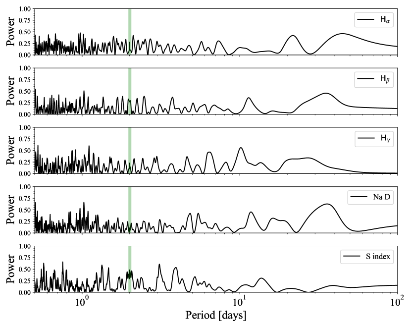
Figure 13: GLS periodograms for the activity indices obtained from 17 HARPS spectra. The period of the planet candidate is shown by the vertical green line.

We find no signals in the RV or activity indices periodograms that points to the rotational period of the star (see Fig. 13). M dwarfs can have rotational periods ranging from a few hours to over one hundred days (e.g., Newton et al., 2016) and our total baseline of HARPS observations is of $\sim 54$ days (with 17 individual spectra). In section 3.1 we derived a rotational period for the host star of $P_{\rm rot}=52\pm 5$ days from empirical relations, hence it is possible that we barely observed a single full rotational period of the star during the spectroscopic follow-up of TOI-674.

3.3 Transit light curve and radial velocity model

The light curves were modeled with the help of the transit modeling package PyTransit (Parviainen, 2015) version 2.0. We used the PyTransit model implementation of the Mandel & Agol (2002) analytic transit model with a quadratic limb darkening law.

Due to the large number of data points, the Spitzer and ground based light curves were detrended before performing the joint fit to speed up the fitting process. For the Spitzer time series we performed Pixel Level Decorrelation (PLD) following Deming et al. (2015) to remove the instrumental noise known to affect Spitzer data. We computed the normalized pixel intensities for each of the $3\times 3$ Spitzer pixels

$$\hat{P}_{i}^{t}=\frac{P_{i}^{t}}{\sum_{i=1}^{N}P_{i}^{t}}$$ (1)

where $P_{i}^{t}$ is the $i$-th pixel inside the aperture at a time $t$ of the time series. We modeled the total flux inside an aperture as

$$S^{t}=\sum_{i=1}^{N}c_{i}\hat{P}_{i}^{t}+T(t)+ft+gt^{2}$$ (2)

where $c_{i}$ are weighting coefficients for the normalized pixel intensities $\hat{P}_{i}^{t}$, $T(t)$ is the transit model, and $ft+gt^{2}$ is a quadratic function in time with constants $f$ and $g$. We fitted the Spitzer time series using equation 2 and compute the $\chi^{2}$ for different aperture sizes and binning the data in time with several bin sizes. The combination of aperture and bin sizes that delivered the lowest $\chi^{2}$ value was used for the global fit.

The ground based light curves were fitted simultaneously using a common transit model and the systematic effects of each data set were accounted for using a linear model with two free parameters dependent on the star position in the detector (X and Y-axis), a term dependent on the Full Width at Half Maximum (FWHM) of the PSF as a proxy for seeing variations, and a time-dependent term to model any time-dependent slope present in the time series.

For the joint fit, the global free parameters for the transit modeling included the planet-to-star radius ratio $\mathrm{R}_{\mathrm{p}}/\mathrm{R}_{\star}$, the central time of the transit $\mathrm{T}_{\mathrm{c}}$, the stellar density $\rho_{\star}$, and the transit impact parameter $\mathrm{b}$. The quadratic limb darkening (LD) coefficients $\mathrm{u}_{1}$ and $\mathrm{u}_{2}$ were set free, but during the fit these values were compared to the predicted coefficients computed for each bandpass using ldtk (Parviainen & Aigrain, 2015). Ldtk uses the Husser et al. (2013) spectral library to compute custom stellar limb darkening profiles. For each light curve the predictd quadratic LD coefficients were computed using the stellar parameters derived in section 3.1 and the fitted coefficients were weighted against these predicted values using a likelihood function. During the fitting process we converted the LD coefficients $(\mathrm{u}_{1},\mathrm{u}_{2})$ to the parameterization proposed by Kipping (2013) $(\mathrm{q}_{1},\mathrm{q}_{2})$ with $q_{i}\in[0,1]$.

For the TESS time series, besides using an analytical model for the transit we fitted the stellar variability present in the time series using Gaussian Processes (GPs; e.g., Rasmussen & Williams, 2010, Gibson et al., 2012, Ambikasaran et al., 2015). The TESS GPs were computed using the python package Celerite (Foreman-Mackey et al., 2017); we chose a Matern $3/2$ kernel:

$$k_{ij\;\mathrm{TESS}}=c^{2}_{1}\left(1+\frac{\sqrt{3}|t_{i}-t_{j}|}{\tau_{1}}\right)\exp\left(-\frac{\sqrt{3}|t_{i}-t_{j}|}{\tau_{1}}\right)$$ (3)

where $|t_{i}-t_{j}|$ is the time between points in the series, $c_{1}$ is the amplitude of the variability, and $\tau_{1}$ is a characteristic time-scale. The constants $c_{1}$ and $\tau_{1}$ were set as free parameters.

The radial velocity data was modeled using RadVel (Fulton et al., 2018). The free parameters in the radial velocity fit were the planet induced radial velocity semi-amplitude ($K_{\mathrm{RV}}$), the host star systemic velocity ($\gamma_{0}$), the instrumental radial velocity jitter ($\sigma_{\mathrm{RV\;jitter}}$), while the orbital period and central transit time were also set free but taken to be global parameters in common with the fits of the light curves. To account for systematic noise present in the radial velocity time series we use GPs with an exponential squared kernel (i.e., a Gaussian kernel)

$$k_{ij\;\mathrm{RV}}=c^{2}_{2}\exp\left(-\frac{(t_{i}-t_{j})^{2}}{\tau^{2}_{2}}\right)$$ (4)

where $t_{i}-t_{j}$ is the time between points in the series, $c_{2}$ is the amplitude of the exponential squared kernel, and $\tau_{2}$ is a characteristic time-scale. The constants $c_{2}$ and $\tau_{2}$ were set as free parameters.

In order to estimate the fitted parameter values we employed a Bayesian approach. We started the fitting procedure by doing an uninformative transit search in the TESS time series (from Sector 9 and 10) using Transit Least Squares (TLS, Hippke & Heller, 2019). From TLS we obtained an estimate of the period and epoch of the central time of the transit with their respective uncertainties, we used these values as priors for the joint fit. Then, we implemented a Markov chain Monte Carlo (MCMC) procedure using emcee (Foreman-Mackey et al., 2013) to evaluate a likelihood plus a prior function. The likelihood function was the sum of the log likelihood for each transit time series and the log likelihood of the radial velocity observations. A total of 38 free parameters were sampled in the joint fit.

The fitting procedure started with a global maximization of the posterior function using PyDE. Once the minimization converged we launched a burn-in MCMC with 125 chains and 2000 iterations. After this burn-in stage was finished, the main MCMC ran for 5000 iterations with the same number of chains as the burn-in stage. The final parameter values and 1$-\sigma$ uncertainties were determined from the posterior distributions of the fitted variables: we computed the percentiles of the distribution corresponding to the median and lower and upper 1-$\sigma$ limits (from the median) of the distribution for each variable.

A planet in such a short orbital period ($P\sim 1.9$ days) is likely to have had its orbit circularized over time. However, this is not necessarily true. There is evidence that Neptune-mass planets with orbital periods of the order of a few days present non-zero orbital eccentricity (e.g., Kane et al., 2012, Correia et al., 2020). Thus, we performed two global fits: one assuming a circular orbit and the other allowed the orbit to have non-zero eccentricity. For the case of the eccentric orbit we set as global free parameters the square root of the eccentricity multiplied by the sine of the argument of the periastron (i.e., $\sqrt{e}\sin(\omega)$ with parameter limits $[-1,1]$) and the square root of the eccentricity multiplied by the cosine of the argument of the periastron (i.e., $\sqrt{e}\cos(\omega)$ with parameter limits $[-1,1]$). Using this parametrization we are sampling values of $e\in[0,1]$ and $\omega\in[0,2\pi]$ (after imposing $e<1$).

Table 4 presents the prior functions and limits used in both global fits. For the circular orbit case we used an uninformative prior (uniform) for the stellar density, with $\rho_{\star}\in[5,15]$ g cm^-3. For the fit allowing a non-zero eccentricity, we imposed a more restrictive range of values for the stellar density, using a normal prior with the density and 2-$\sigma$ uncertainty found by our procedure used to obtain the stellar parameters (see Section 3.1).

4 Results and discussion

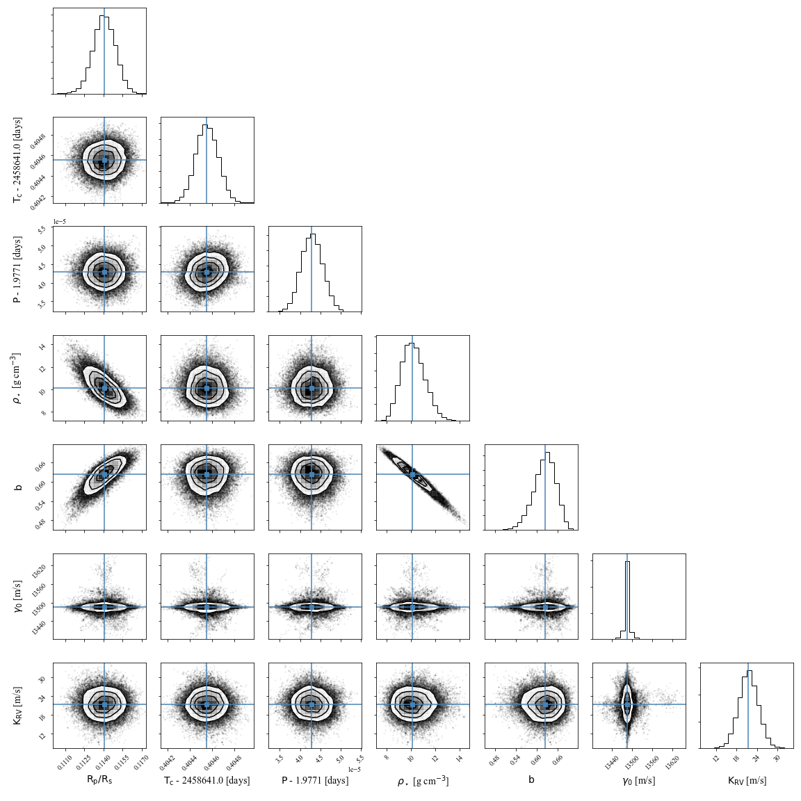
Figure 14: Correlation plot for the orbital parameters fitted using a circular orbit model. Limb darkening coefficients and systematic effect parameters were left out intentionally for easy viewing. The blue lines mark the median values of the parameters.

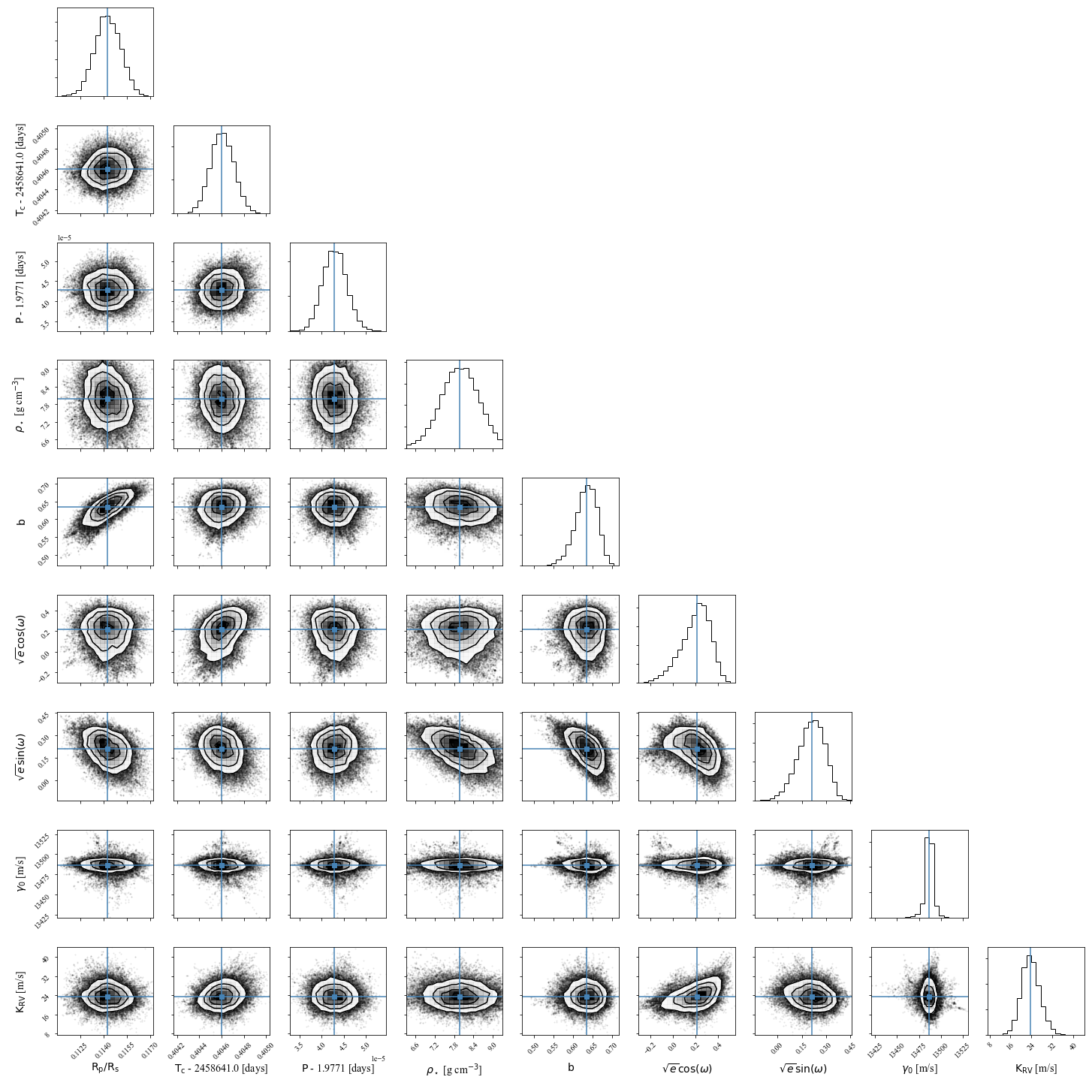
Figure 15: Correlation plot for the orbital parameters fitted using a non-zero eccentricity orbit model. Limb darkening coefficients and systematic effect parameters were left out intentionally for easy viewing. The blue lines mark the median values of the parameters.

The global fit parameter values and 1-$\sigma$ uncertainties are presented in Table 2. Figures 14 and 15 present the correlation plots of the orbital fitted parameters excluding the limb darkening coefficients and parameters related to the red noise. Figures 5 and 6 show all the light curves included in this study and the radial velocity measurements made by HARPS; the best circular orbit model fit from our joint modeling is shown in red.

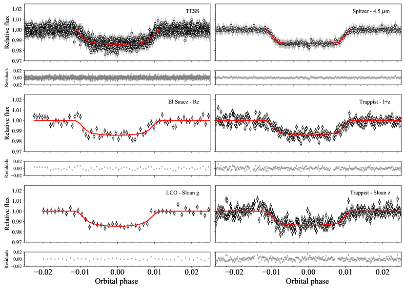
Figure 5: TOI-674b space and ground-based transit light curves after removing systematic noise affecting the data. The best circular orbit model fit is represented by the red line and below each panel the residuals of the fit are shown.

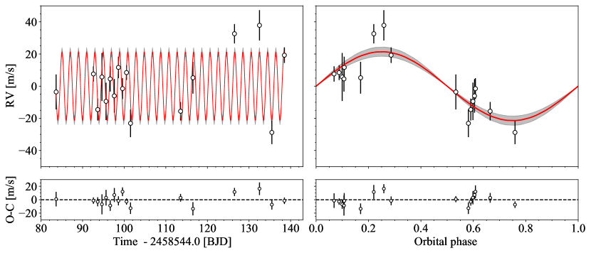
Figure 6: TOI-674b HARPS radial velocity measurements and best fitting circular orbit model including Gaussian processes to model systematic noise sources (red line). Left: HARPS RV time series measurements. Right: HARPS RV measurements phase-folded to the orbital period of the planet.The shaded gray area corresponds to $\pm 1$-$\sigma$ level from the mean of 5000 randomly selected posterior samples. The RMS of the residuals is $8.25$ m/s.

Table 2: TOI-674b global fit parameters and 1-$\sigma$ uncertainties for the circular and non-zero eccentricity fits. The prior functions and parameter limits used in the joint fit are presented in Table 4. The adopted stellar mass and radius used to derive the absolute planet parameters are the ones presented in the middle column of Table 1 (i.e., BT-Settl models SED fit).

Fitted orbital parameter	Circular orbit ($e=0$)	Non circular orbit ($e\neq 0)$
$R_{p}/R_{\star}$	$0.1140\pm 0.0009$	$0.1143\pm 0.0009$
$T_{\mathrm{c\;BJD}}$ [days]	$2458641.404552\pm 0.000102$	$2458641.404604\pm 0.000108$
$P$ [days]	$1.977143\pm 0.000003$	$1.977143\pm 0.000003$
$\rho_{\star}$ [g cm-3]	$10.14\pm 1.04$	$7.97\pm 0.59$
$b=(a/R_{\star})\cos(i)\left(\frac{1-e^{2}}{1+e\sin(\omega)}\right)$	$0.624\pm 0.035$	$0.635\pm 0.030$
$\sqrt{e}\cos(\omega)$	—-	$0.217\pm 0.153$
$\sqrt{e}\sin(\omega)$	—-	$0.211\pm 0.089$
$\gamma_{0}$ [m/s]	$13485.51\pm 4.78$	$13486.59\pm 3.81$
$K$ [m/s]	$21.44\pm 2.94$	$23.55\pm 3.70$
$\sigma_{\mathrm{RV}}$ [m/s]	$3.40\pm 2.95$	$3.58\pm 2.85$
Derived orbital parameters
$e$	—-	$0.10\pm 0.05$
$\omega$ [deg]	—-	$45.4\pm 30.8$
$a/R_{\star}$	$12.80\pm 0.42$	$11.81\pm 0.30$
$i$ [deg]	$87.21\pm 0.24$	$86.68\pm 0.20$
Fitted LD coefficients
$\mathrm{u}_{\mathrm{1\;TESS}}$	$0.25\pm 0.13$	$0.24\pm 0.13$
$\mathrm{u}_{\mathrm{2\;TESS}}$	$0.36\pm 0.19$	$0.36\pm 0.17$
$\mathrm{u}_{\mathrm{1\;4.5\mu m}}$	$0.071\pm 0.036$	$0.073\pm 0.043$
$\mathrm{u}_{\mathrm{2\;4.5\mu m}}$	$0.15\pm 0.07$	$0.15\pm 0.07$
$\mathrm{u}_{\mathrm{1\;R_{c}}}$	$0.29\pm 0.18$	$0.30\pm 0.17$
$\mathrm{u}_{\mathrm{2\;R_{c}}}$	$0.42\pm 0.26$	$0.41\pm 0.24$
$\mathrm{u}_{\mathrm{1\;I+z}}$	$0.24\pm 0.13$	$0.23\pm 0.14$
$\mathrm{u}_{\mathrm{2\;I+z}}$	$0.36\pm 0.19$	$0.36\pm 0.19$
$\mathrm{u}_{\mathrm{1\;g}}$	$0.48\pm 0.26$	$0.48\pm 0.24$
$\mathrm{u}_{\mathrm{2\;g}}$	$0.38\pm 0.30$	$0.38\pm 0.29$
$\mathrm{u}_{\mathrm{1\;z}}$	$0.38\pm 0.13$	$0.39\pm 0.15$
$\mathrm{u}_{\mathrm{2\;z}}$	$-0.01\pm 0.19$	$-0.04\pm 0.21$
TESS GP parameters
$\mathrm{c}_{1}$	$(2.1\pm 0.4)\times 10^{-4}$	$(2.1\pm 0.4)\times 10^{-4}$
$\tau_{1}$ [days]	$0.74\pm 0.30$	$0.75\pm 0.35$
HARPS GP parameters
$\mathrm{c}_{2}$ [m/s]	$4.3^{+9.9}_{-3.2}$	$3.3^{+5.5}_{-2.4}$
$\tau_{2}$ [days]	$49\pm 31$	$45\pm 30$
Derived planet parameters
$\mathrm{R}_{\mathrm{p}}$ [$\mathrm{R}_{\oplus}$]	$5.25\pm 0.17$	$5.26\pm 0.17$
$\mathrm{M}_{\mathrm{p}}$ [$\mathrm{M}_{\oplus}$]	$23.6\pm 3.3$	$23.5\pm 3.3$
$\rho_{\mathrm{p}}$ [g cm-3]	$0.91\pm 0.15$	$0.90\pm 0.15$
$\mathrm{g}_{\mathrm{p}}$ [m s-2]	$8.5\pm 1.3$	$8.4\pm 1.3$
$\mathrm{a}$ [AU]	$0.0250\pm 0.0008$	$0.0231\pm 0.0007$
$\mathrm{T}_{\mathrm{eq}}$ [K]	$635\pm 15$	$661\pm 14$
$\langle\mathrm{F}_{\mathrm{p}}\rangle$ [105 W/m2]	$0.523\pm 0.039$	$0.612\pm 0.045$
$\mathrm{S}_{\mathrm{p}}$ [$\mathrm{S}_{\odot}$]	$38.73\pm 2.88$	$45.48\pm 3.39$

4.1 The orbital eccentricity of TOI-674b

By using a normal prior on the stellar density with the values taken from the stellar parameters for the host star and setting the eccentricity and argument of the periastron free, we find that TOI-674b may have a slightly eccentric orbit with $\mathrm{e}=0.10\pm 0.05$, although this eccentricity value could be an spurious signal. According to Lucy & Sweeney (1971), an eccentricity should not be considered significant if it is less than 2.45$\sigma$ from zero, which our eccentric fit does not achieve. Nonetheless, many Neptune-mass planets with short orbital periods posses non-circular orbits like HAT-P-11b (Bakos et al., 2010, Yee et al., 2018), GJ 436b (Gillon et al., 2007, Lanotte et al., 2014), and TOI-1728b (Kanodia et al., 2020) to name some examples. Correia et al. (2020) proposed that these non-circular orbits could be produced by any of several processes alone or in combination like a tidal torque created by photo-driven evaporation of the planet’s atmosphere and/or gravitational interaction between the short period planet and another planetary object in a longer period orbit in the system.

We compared the Bayesian Information Criterion (BIC) statistics of the circular and eccentric orbit model fits to the data. The BIC takes into account the number of observed data points $n$, the number of fitted parameters $k$, and the maximized likelihood $\mathcal{L}_{\mathrm{max}}$. The BIC is defined by

$$\mathrm{BIC}=k\ln{n}-2\ln{\mathcal{L}_{\mathrm{max}}}\;.$$ (5)

The model with the lowest BIC value is the one that better fits the data. In our case $\Delta\mathrm{BIC}=\mathrm{BIC}_{\mathrm{Ecc}}-\mathrm{BIC}_{\mathrm{Circ}}=44$, meaning that the circular model fit is preferred using this criterion.

It is worth pointing out that the stellar density $\rho_{\star}$, transit impact parameter $\mathrm{b}$, eccentricity $\mathrm{e}$, and argument of the periastron $\omega$ are correlated. In our non-zero eccentricity model fit we used a normal prior to the stellar density which could have skewed our results to eccentricity values higher than zero. Another point to consider is that our radial velocity measurements were made with a rather nonuniform distribution in orbital phase, in part due to the orbital period being almost an integer number of days ($P\sim 1.9$ days) making a uniform coverage difficult from a single observing site. The non-uniform phase coverage contributes to the difficulty of establishing whether the orbit is slightly eccentric. Additional RV measurements in different orbital phases and/or observations with higher precision, for example using VLT/ESPRESSO (Pepe et al., 2010, 2021), could help to put stronger constraints on the orbital eccentricity of TOI-674b.

On the other hand, the stellar density found by our circular orbit fit using a uniform prior for this parameter is $\rho_{\star}=10.14\pm 1.04$ g cm^-3, a value that differs from the derived stellar density computed using our adopted stellar mass and radius ($\rho_{\star}=7.99\pm 0.76$ g cm^-3) by $\sim 2\sigma$. This discrepancy could be caused by an underestimation of the uncertainties of the stellar parameters or an unknown systematic affecting our fit. The different stellar density values found in the circular and non-circular orbit fit affected the values of the semi-major axis over stellar radius ($a/R_{\star}$) and orbital inclination ($i$) (see Table 2) since these values were derived using the stellar density, impact parameter, eccentricity and argument of the periastron.

Despite the different values of stellar density from our circular and non-zero eccentricity results, both cases are in agreement within the 1-$\sigma$ uncertainties (see Table 2). Given the BIC results, for the rest of this work we will adopt the planetary parameters derived from the circular orbit model fit.

4.2 Transit timing variations

The presence of additional planets in the system could perturb the orbit of TOI-674b and produce an orbit with non-zero eccentricity. The interactions between TOI-674b and these hypothetical additional planets in the system could also affect the central times of the observed transits. We searched for transit timing variations (TTVs) of TOI-674b by fitting the TESS photometry from Sector 9 and Sector 10, the Spitzer transit, and the 4 ground-based transits jointly with PyTTV (Korth, 2020). This translated into 27 individual transit fits spanning a time baseline of close to $\sim 200$ days. The fitted model included individual transit centers as free parameters and shared the remaining geometric and orbital parameters such as impact parameter, radius ratio, and stellar density. We estimated the model parameter posteriors using MCMC-sampling (emcee; Foreman-Mackey et al., 2013). The transit centers do not show significant variations from the linear ephemeris. We show the TTVs in Fig. 7.

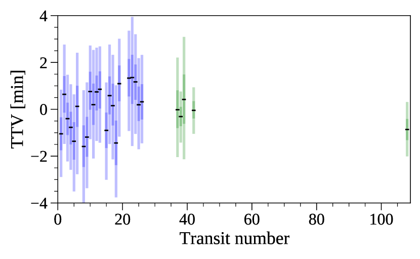
Figure 7: TOI-674b transit timing variations from TESS data (blue) and follow-up observations (green). The different shades of color of the error bars represent the 1-$\sigma$ (dark) and 3-$\sigma$ (light) levels of uncertainty of the measurements. No significant TTVs are detected in a $\sim 200$ days of baseline covered by the observations.

The photometric measurements do not cover a long enough period ($\sim 200$ days) to allow us to put further constraints on hypothetical additional planets in the system which could be responsible for an eccentric orbit of TOI-674b via gravitational interactions. Further monitoring (spectroscopic and photometric) is therefore desirable.

4.3 Mass, radius and composition

We find that TOI-674b has a radius of $5.25\pm 0.17$ $\mathrm{R}_{\oplus}$ and a mass of $23.6\pm 3.3$ $\mathrm{M}_{\oplus}$. Combining these measurements we find that TOI-674b has a mean density of $\rho_{\mathrm{p}}=0.91\pm 0.15$ g cm^-3.

We compared the mass and radius of TOI-674b with known exoplanets taken from the TEPcat database (Southworth, 2011) and the composition models of Zeng et al. (2019). The planet models consider an isothermal atmosphere and are truncated at 1 milli-bar pressure level (defining the radius of the planet). Figure 8 shows the mass-radius diagram for known transiting exoplanets with masses measured with a precision better than 30% and the rocky planet models of Zeng et al. (2019) with an equilibrium temperature of 700 K, i.e., the equilibrium temperature closest to the likely temperature of TOI-674b. The planet models shown in Fig. 8 are planets with pure iron cores (100% Fe), earth-like rocky compositions (32.5% Fe plus 67.5% MgSiO₃), a 100% water compositions, and earth-like composition planet cores with 5% H₂ gaseous envelopes. We can see that TOI-674b is located far above all of these model predictions, suggesting that this planet must possess a very large H/He envelope.

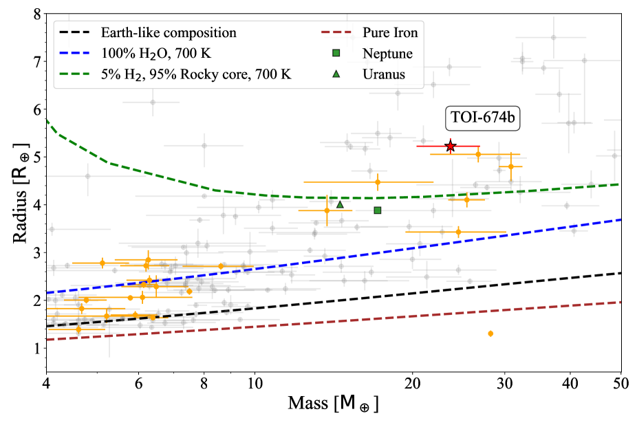
Figure 8: Mass-radius diagram for planets with mass determinations with a precision better than 30%. The red star is TOI-674b, the orange points are planets orbiting M type stars, and the gray points are planets around other types of stars. The dashed lines represent the mass-radius models of Zeng et al. (2019): planets with pure iron cores (100% Fe, brown line), earth-like rocky compositions (32.5% Fe plus 67.5% MgSiO₃, black line), 100% water compositions (blue line), and earth-like composition planet cores with 5% H₂ gaseous envelopes (green line).

Comparing the mass and radius of TOI-674b with other planets discovered orbiting around M type stars, we find that TOI-674b is one of the largest and most massive super-Neptune class planets discovered around an M-dwarf to date. The planets orbiting M-dwarfs closest to TOI-674b in the M-R diagram are TOI-1728b (Kanodia et al., 2020) and TOI-442b (Dreizler et al., 2020). TOI-1728b orbits an M0V star ($\mathrm{T}_{\mathrm{eff}}=3980$ K) and is a super-Neptune with $\mathrm{R}_{\mathrm{p}}=5.05\pm 0.17$ $\mathrm{R}_{\oplus}$, $\mathrm{M}_{\mathrm{p}}=26.78\pm 5.43$ $\mathrm{M}_{\oplus}$ and an orbital period of $\sim 3.5$ days ($\mathrm{T}_{\mathrm{eq}}=767$ K). TOI-442b is another Neptune-like planet orbiting an M0V star with $\mathrm{R}_{\mathrm{p}}=4.7\pm 0.3$ $\mathrm{R}_{\oplus}$, $\mathrm{M}_{\mathrm{p}}=30.8\pm 1.5$ $\mathrm{M}_{\oplus}$, and an orbital period of $\sim 4$ days. TOI-674b, TOI-1728b and TOI-442b have very similar masses and radii; neither planet has a very eccentric orbit. All host stars are main-sequence M dwarfs, but the star TOI-674 is smaller and less luminous than TOI-1728 and TOI-442, therefore even though its planet has a closer-in orbit, it has a slightly smaller equilibrium temperature (for the same albedo). The similarity between these three recent TESS discoveries means that most of the qualitative information in the Discussion and Summary sections of Kanodia et al. (2020) and Dreizler et al. (2020) also applies to TOI-674b.

The voluminous envelope of TOI-674b suggests that it has more H₂ than could be obtained from accretion and degassing of solid material (Rogers et al., 2011); therefore it must have accreted gas directly from its protoplanetary disk. Accretion of large gaseous envelopes so close to a star requires a very massive solid core, so this planet very likely formed much farther from its star and then moved inwards, either via gradual disk migration early in the system’s history when the protoplanetary disk was still massive or later via high-eccentricity migration and tidal circularization. Early arrival at its current orbit would have subjected TOI-674b to a long epoch of substantial photoionizing radiation, stripping the outer part of the atmosphere; tidal heating would also have induced substantial mass loss. Thus, TOI-674b probably formed with a substantially more massive envelope that was partially stripped away, mostly in the first tens of millions of years after reaching its current orbit (e.g., check Fulton et al., 2017, Fulton & Petigura, 2018 and references therein).

4.4 TOI-674b and the Neptunian desert

Based on our derived mass and orbital period, TOI-674b is a new resident of the so-called Neptunian Desert. In Figure 9 we plotted the $\log\mathrm{P}$ vs $\log\mathrm{M_{p}}$ relationship for known exoplanets; the black lines are the limits of the Neptunian Desert by Mazeh et al. (2016). TOI-674b is well within the limits of the desert and in a region sparsely populated in the orbital period versus radius space.

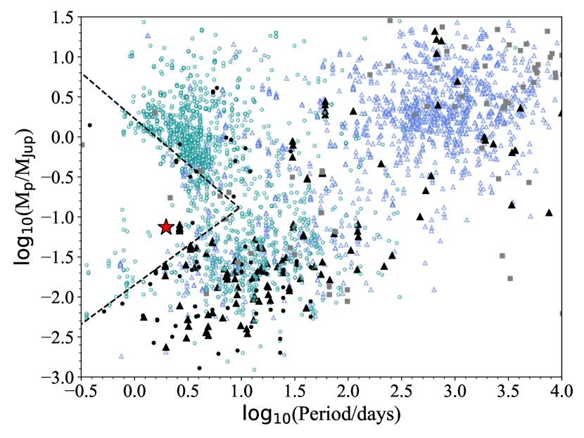
Figure 9: Mass versus orbital period diagram for planets with mass measurements. Planets found by the transit method are shown in light cyan circles, planets found by radial velocity measurements are shown in blue triangles, and planets found by other methods are shown in gray squares. The filled black symbols represent planets orbiting around M stars (i.e, stars with $\mathrm{T}_{\mathrm{eff}}$ in the range 2500-4000 K), each symbol representing the discovery method as explained before. The black dashed lines represent the limits of the Neptunian Desert defined by Mazeh et al. (2016). TOI-674b position in this diagram is marked by the red star.

There are multiple scenarios that explain the origin of the Neptunian desert. One proposed explanation of the lack of Neptune-sized planets in short orbits is photo-evaporation of the planet’s H/He envelope due to high energy radiation coming from the star once the planet arrives to a position close to its central star after formation (e.g., Owen & Wu, 2013, Lopez & Fortney, 2013, Chen & Rogers, 2016). The lower boundary of the desert in Mazeh et al. (2016) (i.e., planets with low mass/small radius) is consistent with this proposed photo-evaporation mechanism. Matsakos & Königl (2016) proposed that tidal disruption of planets in highly-eccentric orbits (followed by circularisation of the orbit due to tidal interactions with the host star) can explain both boundaries of the desert. Owen & Lai (2018) proposed that both mechanisms are able to explain the Neptunian desert, with photo-evaporation creating the low mass/small radius and high mass/large radius boundary being created by the tidal disruption limit for gas giants experiencing high-eccentric migration. Although TOI-674b is inside the proposed boundary by Mazeh et al. (2016), it is closer to the low mass/small radius limit indicating that this planet may have experienced some photo-evaporation of its upper atmospheric layers due to the high energy radiation of its host star.

It is also worth noting that there are few large planets known to orbit M stars. Bonfils et al. (2013) estimated the occurrence of planets around M dwarfs using HARPS data and showed that planets with large masses were not common around these types of stars. Bonfils et al. (2013) found that the occurrence for planets with $\mathrm{M}_{\mathrm{p}}\sin(i)$ in the range of [10, 100] $\mathrm{M}_{\oplus}$ and with orbital periods shorter than 10 days is $0.03^{+0.04}_{-0.01}$. A similar result was obtained by Dressing & Charbonneau (2015) using Kepler data to estimate the rate of planets around M stars. For the largest planet size range studied by Dressing & Charbonneau (2015), i.e., $\mathrm{R}_{\mathrm{p}}\in[3.5,4.0]$ $\mathrm{R}_{\oplus}$ and orbital periods shorter than 50 days, Dressing & Charbonneau (2015) find an occurrence rate of $0.016^{+0.018}_{-0.070}$ planets per M dwarf.

4.5 Potential for atmospheric characterisation

Due to the large scale height of its atmosphere and relative brightness of its host star in near infrared bands, TOI-674b is a promising target for atmospheric studies. Kempton et al. (2018) proposed a metric for the expected S/N of transmission spectroscopy with the James Webb Space Telescope (JWST, Gardner et al., 2006) instrument Near Infrared Imager and Slitless Spectrograph (NIRISS) for 10 hours of observation time. Following Kempton et al. (2018), we find a Transmission Spectroscopy Metric (TSM) of $\sim 230$ for TOI-674b. We compared this TSM value with those of previously discovered exoplanets that are in the Neptunian Desert (see Figure 10). TOI-674b is one of the planets belonging to the Neptunian Desert with the highest TSM factor discovered to date, making it an interesting candidate for atmospheric characterisation for JWST.

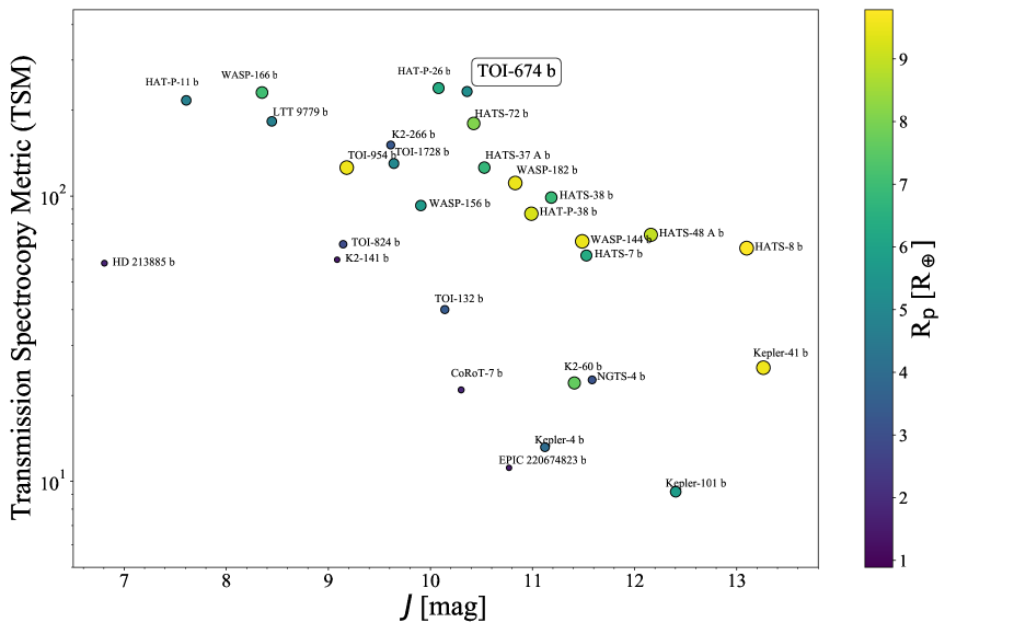
Figure 10: Apparent magnitude in J band versus the Transmission Spectroscopy Metric (TSM) by Kempton et al. (2018) for TOI-674b and known transiting super-Earths and Neptune-sized planets inside the Neptunian Desert limits by Mazeh et al. (2016). The size and color of each circle represents the planet radius in Earth units.

We computed a synthetic transmission spectrum of TOI-674b using petitRADTRANS (Mollière et al., 2019). The model spectrum assume solar elemental abundances and a cloud-free atmosphere with an isothermal temperature profile at a temperature of 700 K. Figure 11 presents model optical and infrared spectra potentially observable with JWST for an assumed atmospheric pressure level of 0.01 bar for the continuum. The atmosphere models include molecules such as H₂O, CO₂, CO, CH₄, and Na and K; Rayleigh scattering from H and He is also included.

Figure 11 also shows simulated observations made with JWST of the model spectrum. The simulations were made for the JWST instruments Near Infrared Imager and Slitless Spectrograph (NIRISS) using Single Object Slitless Spectroscopy (SOSS) mode (spectral resolution $\mathrm{R}\sim 700$), Near InfraRed Spectrograph (NIRSpec) using the medium resolution grating G395M ($\mathrm{R}\sim 1000$), and Mid-Infrared Instrument (MIRI) using Low Resolution Spectroscopy (LRS) mode ($\mathrm{R}\sim 100$). The simulated observations cover a wavelength range of 0.8-10 $\mu$m.

For the JWST simulated data we used ExoTETHyS.BOATS (Morello et al., 2021) to select wavelength bins with similar number of counts, in order to have comparable error bars from each point of the spectrum. Using a constant resolution, or a fixed bin width ($\Delta\lambda$), would increase the error bars and the scatter in some spectral regions by a factor of several units, especially in the MIRI longer wavelengths. Although the total integrated S/N is independent on the choice of bins, a higher scatter per point may hinder the detection significance of broad molecular features (e.g., Tsiaras et al., 2018). Then, we recomputed the spectra with PandExo (Batalha et al., 2017), which fully accounts for the specific JWST instrument modes. We noted that the spectra simulated with ExoTETHyS.BOATS and PandExo are consistent, including their error bars. The main differences appear to be related with the adopted stellar templates. Here, we show only the results obtained with PandExo. It is remarkable that all the various H₂O and CH₄ features can be well sampled by ¿10 points with order-of-magnitude smaller error bars than the amplitude of the features (for a cloud-free atmosphere).

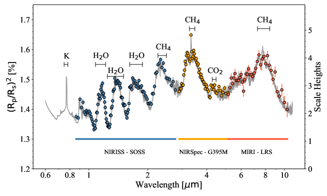
Figure 11: Synthetic transmission spectrum model of TOI-674b (gray line) in the JWST spectral range computed with petitRADTRANS (Mollière et al., 2019). The model assumes solar abundance and a cloud-free atmosphere with an isothermal temperature of 700 K. PandExo (Batalha et al.) simulations of TOI-674b transmission spectrum observations made with JWST instruments NIRISS (blue), NIRSpec (orange), and MIRI (red) are also shown.

It should be noted that the cloud-free transmission spectrum presented here is the most optimistic scenario. Transmission spectroscopy studies done in mostly hot-Jupiters have shown that many planets posses molecular features with a lower amplitude than what the cloud-free models predict (e.g., Sing et al., 2011, Deming et al., 2013, Kreidberg et al., 2014). This lack of molecular traits is often explained by the presence of clouds and hazes dampening the strength of the expected features like, for example, the case of water bands in the near-infrared for hot-Jupiters (Sing et al., 2016). Thus, it would be preferable to establish if TOI-674b atmosphere is cloud-free with exploratory transmission spectroscopy observations before JWST is operational. Optical low resolution observations could detect evidence for Rayleigh scattering and the broad wings of Na and K lines (e.g., Nikolov et al., 2018), although the detection of the latter lines would be challenging due to the relative faintness (for these type of studies) of the planet host star ($V=14.2$ mag). In the near-infrared it would be possible to use Hubble Space Telescope (HST) Wide Field Camera 3 (WFC3) to detect the water bands between 1.0-1.7 $\mu$m as shown by several studies (e.g., Wakeford et al., 2013, Madhusudhan et al., 2014, Sing et al., 2016 , Tsiaras et al., 2018).

Another interesting prospect for atmosphere characterisation is to search for evidence of atmospheric escape using individual lines of hydrogen (Lyman-$\alpha$, 121.5 nm) and helium (He I triplet at 1083 nm). These lines have been detected on short-period warm Neptunes orbiting around M dwarfs like for example GJ 436b (Lyman-$\alpha$, Ehrenreich et al., 2015) and GJ 3470b (He I, Palle et al., 2020).

5 Conclusions

We report the discovery and confirm the planetary status of TOI-674b, a super-Neptune transiting exoplanet orbiting around a nearby M dwarf. NASA’s TESS observations led to the initial detection of the transits. Follow-up photometric observations made with several facilities and radial velocity measurements taken with the HARPS spectrograph made possible confirmation of the planetary nature of the transiting object and establishment of its mass and radius.

From a HARPS mean stellar spectrum we estimate that the spectral type of the host star is M2V and that the star has an effective an effective temperature of $\mathrm{T}_{\mathrm{eff}}=3514\pm 57$ K, and a stellar mass and radius of $\mathrm{M}_{\star}=0.420\pm 0.010$ $\mathrm{M}_{\odot}$ and $\mathrm{R}_{\star}=0.420\pm 0.013$ $\mathrm{R}_{\odot}$ respectively.

We analysed the data from Sector 9 and 10 two minute cadence time series observations from TESS (PDCSAP curves) plus single transit follow-up observations from Spitzer Space Telescope ($4.5\;\mu\mathrm{m}$ band), and ground-based facilities: El Sauce ($\mathrm{R}_{\mathrm{c}}$ filter), LCOGT (Sloan-g filter), and TRAPPIST-South telescopes ($I+z$, Sloan-z bands). The single transit observations were detrended before performing a global joint fit of the data in order to reduce the number of free parameters and speed up the fitting procedure. The transit observations (TESS time series plus single transit follow-up observations) and radial velocity measurements from HARPS were fitted simultaneously using a MCMC procedure that included Gaussian processes to model the systematic effects present in TESS and RV measurements. For the joint fit we considered two cases to determine the orbital parameters of the planet: a circular orbit and a non-zero eccentricity model.

For both fitted models (circular and eccentric model), we find that the derived planetary mass and radius agree within uncertainties. The non-zero eccentric solution presents an eccentricity value of $e=0.10\pm 0.05$, hence this planet could potentially join the previous known short period Neptune-sized planets with significant eccentricities. Since most of our radial velocity measurements were made during quadrature, more follow-up observations can help to further constraint the eccentricity value for this planet.

Using our circular orbit model fit we find that TOI-674b has a radius of $\mathrm{R}_{\mathrm{p}}=5.25\pm 0.17$ $\mathrm{R}_{\oplus}$ and a mass of $\mathrm{M}_{\mathrm{p}}=23.6\pm 3.3$ $\mathrm{M}_{\oplus}$, and it orbits its star with a period of $1.977143\pm 3\times 10^{-6}$ days. We derived a mean bulk density of $\rho_{\mathrm{p}}=0.91\pm 0.15$ g cm^-3, indicating a large atmosphere/envelope. Comparing the mass and radius of TOI-674b with literature values for planets discovered orbiting around M type stars, we find that TOI-674b is one of the largest and most massive super-Neptune class planet discovered around an M-dwarf to date.

This planet is a new addition to the so-called Neptunian Desert. The Transmission Spectroscopy Metric (TSM) of TOI-674b is $\sim 240$, one of the highest TSM for Neptunian Desert planets. Thus, TOI-674b is a promising candidate for atmospheric characterisation using JWST.

We searched for evidence of another planets in the system by measuring the transit timing variations using the data from TESS, Spitzer, and ground-based follow-up observations. We find no significant deviations from a linear ephemeris for the central time of the transits in a time baseline of $\sim 200$ days. TOI-674 is expected to be observed again by TESS during its extended campaign. The observations will be done from 7 March 2021 until 2 April 2021 (corresponding to Sector 36); these new TESS observations will help to refine TOI-674b’s orbital parameters and in the search for additional planets in the system.

Appendix A Spectral energy distribution of TOI-674

Appendix B Spectroscopic data measurements

Table 3: HARPS radial velocity time series and spectroscopic activity indicators for TOI-674.

BJD [-245800]	RV [ms-1]	$\sigma_{\mathrm{RV}}$ [ms-1]	$\mathrm{H}_{\alpha}$	$\sigma_{\mathrm{H_{\alpha}}}$	$\mathrm{H}_{\beta}$	$\sigma_{\mathrm{H_{\beta}}}$	$\mathrm{H}_{\gamma}$	$\sigma_{\mathrm{H_{\gamma}}}$	NaD	$\sigma_{\mathrm{NaD}}$	S	$\sigma_{\mathrm{S}}$
8627.630457	13481.91	10.85	0.0692	0.0014	0.0521	0.0037	0.1076	0.0130	0.0059	0.0021	0.4891	0.6417
8636.597318	13493.11	04.75	0.0675	0.0006	0.0495	0.0017	0.1085	0.0064	0.0076	0.0008	1.1554	0.3996
8637.628554	13470.93	06.80	0.0670	0.0008	0.0550	0.0028	0.1026	0.0106	0.0075	0.0012	0.7150	0.5353
8638.635832	13491.23	14.92	0.0668	0.0018	0.0503	0.0063	0.1001	0.0204	0.0069	0.0030	1.3946	0.8684
8639.622186	13476.06	11.65	0.0663	0.0014	0.0486	0.0050	0.1009	0.0161	0.0087	0.0022	0.4529	0.7547
8640.626096	13490.04	07.86	0.0679	0.0010	0.0452	0.0031	0.0981	0.0129	0.0081	0.0014	0.8246	0.6512
8641.611199	13479.48	10.45	0.0664	0.0013	0.0477	0.0044	0.1143	0.0192	0.0061	0.0020	1.1750	1.1082
8642.605629	13497.19	06.66	0.0677	0.0008	0.0517	0.0030	0.1134	0.0137	0.0083	0.0012	0.9768	0.6242
8643.595060	13483.99	06.48	0.0677	0.0008	0.0507	0.0026	0.1185	0.0103	0.0082	0.0011	0.5704	0.5792
8644.544065	13493.96	04.58	0.0667	0.0006	0.0524	0.0017	0.1264	0.0066	0.0088	0.0007	1.0437	0.4021
8645.519317	13462.41	08.60	0.0696	0.0011	0.0547	0.0030	0.1080	0.0099	0.0098	0.0016	1.0369	0.4539
8657.546337	13469.92	05.71	0.0690	0.0007	0.0602	0.0023	0.1071	0.0077	0.0092	0.0010	0.9712	0.4522
8660.523300	13490.75	09.88	0.0675	0.0012	0.0539	0.0037	0.0863	0.0125	0.0075	0.0019	1.0510	0.7247
8670.508395	13518.13	06.02	0.0692	0.0008	0.0500	0.0023	0.1152	0.0084	0.0072	0.0010	0.6041	0.3814
8676.515917	13523.37	09.43	0.0674	0.0012	0.0455	0.0034	0.1219	0.0121	0.0081	0.0018	1.0161	0.4858
8679.482254	13456.72	07.26	0.0680	0.0008	0.0623	0.0035	0.0900	0.0115	0.0095	0.0013	0.7379	0.4551
8682.501971	13504.79	04.83	0.0670	0.0006	0.0533	0.0018	0.1120	0.0065	0.0090	0.0008	0.8569	0.3134

Appendix C Light curve and radial velocity joint fit

Table 4: Global fit parameters prior functions and limits; $\mathcal{U}$, $\mathcal{N}$, and $\mathcal{J}$ represent Uniform, Normal, and Jeffreys prior functions respectively.

Fitted parameter	Ccircular orbit ($e=0$)	Non-circular orbit ($e\neq 0$)
$R_{\mathrm{p}}/R_{\star}$	$\mathcal{U}(0.05,0.35)$	$\mathcal{U}(0.05,0.35)$
$T_{\mathrm{c\;BJD}}$ [days]	$\mathcal{U}(2458640.9,2458641.9)$	$\mathcal{U}(2458640.9,2458641.9)$
$P$ [days]	$\mathcal{U}(1.7,2.1)$	$\mathcal{U}(1.7,2.1)$
$\rho_{\star}$ [g cm-3]	$\mathcal{U}(5,15)$	$\mathcal{N}(7.99,1.5)$
$b=(a/R_{\star})\cos(i)\left(\frac{1-e^{2}}{1+e\sin(\omega)}\right)$	$\mathcal{U}(0,1)$	$\mathcal{U}(0,1)$
$\sqrt{e}\cos(\omega)$		$\mathcal{U}(-1,1)$
$\sqrt{e}\sin(\omega)$		$\mathcal{U}(-1,1)$
$\gamma_{0}$ [m/s]	$\mathcal{U}(-10^{5},10^{5})$	$\mathcal{U}(-10^{5},10^{5})$
$K_{\mathrm{RV}}$ [m/s]	$\mathcal{U}(0,110)$	$\mathcal{U}(0,110)$
$\sigma_{\mathrm{RV\;jitter}}$ [m/s]	$\mathcal{U}(0,10)$	$\mathcal{U}(0,10)$
LD coefficients
$q_{1}=(u_{1}+u_{2})^{2}$	$\mathcal{U}(0,1)$	$\mathcal{U}(0,1)$
$q_{2}=0.5u_{1}/(u_{1}+u_{2})$	$\mathcal{U}(0,1)$	$\mathcal{U}(0,1)$
TESS GP parameters
$\mathrm{c}_{1}$	$\mathcal{J}(10^{-4},100)$	$\mathcal{J}(10^{-4},100)$
$\tau_{1}$ [days]	$\mathcal{J}(10^{-4},200)$	$\mathcal{J}(10^{-4},200)$
HARPS GP parameters
$\mathrm{c}_{2}$ [m/s]	$\mathcal{U}(0,100)$	$\mathcal{U}(0,100)$
$\tau_{2}$ [days]	$\mathcal{U}(10^{-3},80)$	$\mathcal{U}(10^{-3},80)$

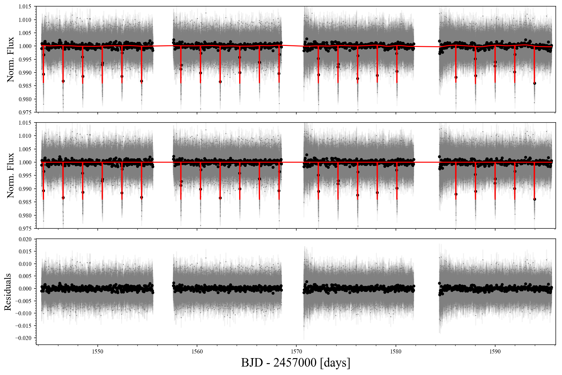
Figure 16: TESS Sector 9 and Sector 10 two minute cadence light curves of TOI-674. Top panel: TESS PDCSAP flux time series and best circular orbit model from the joint fit. Middle panel: TESS flux and transit model after removing stellar variability.Bottom panel: residuals of the fit.