Improved Spanning on Theta-5

Abstract

We show an upper bound of $\frac{\sin\left(\frac{3\pi}{10}\right)}{\sin\left(\frac{2\pi}{5}\right)-\sin\left(\frac{3\pi}{10}\right)}<5.70$ on the spanning ratio of $\Theta_{5}$-graphs, improving on the previous best known upper bound of $9.96$ [Bose, Morin, van Renssen, and Verdonschot. The Theta-5-graph is a spanner. Computational Geometry, 2015.] Keywords: Theta Graphs Spanning Ratio Stretch Factor Geometric Spanners.

1 Introduction

A geometric graph $G$ is a graph whose vertex set is a set of points $P$ in the plane, and where the weight of an edge $uv$ is equal to the Euclidean distance $|uv|$ between $u$ and $v$. Informally, a $\Theta_{k}$-graph is a geometric graph built by dividing the area around each point of $v\in P$ into $k$ equal angled cones, connecting $v$ to the closest neighbor in each cone (we shall define closest later). Such graphs arise naturally in settings like wireless networks, where signals to anyone but your nearest neighbor may be drowned out by interference. Moreover, the fact that signal strength fades quadratically with distance, and thus that power requirements are proportional to the square of the distance the signal has to travel, makes many small hops economically superior to one large hop, even if the sum of the distances is larger. The spanning ratio (sometimes called the stretch factor) of a geometric graph $G$ is the maximum over all pairs $u,v\in P$ of the ratio between the length of the shortest path from $u$ to $v$ in $G$ and the Euclidean distance from $u$ to $v$. Using simple geometric observations and techniques, we give a new analysis of the spanning ratio of $\Theta_{5}$-graphs, bringing down the best known upper bound from $9.96$ [5] to $5.70$. theoremTheoremMain Given a set $P$ of points in the plane, the $\Theta_{5}$-graph of $P$ is a $5.70$-spanner.

(a) Measure of the distance to point $a$.

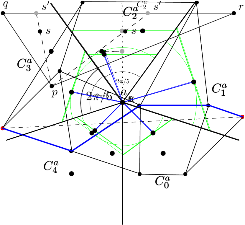
(b) The neighbors of $a$ in the $\Theta_{5}$-graph.

Figure 1: The area around a point $a$ is divided into cones with angle $2\pi/5$.

$\Theta_{k}$-graphs were introduced simultaneously by Keil and Gutwin [8, 9], and Clarkson [7]. Both papers gave a spanning ratio of $1/(\cos\theta-\sin\theta)$, where $\theta=2\pi/k$ is the angle defined by the cones. Observe that this gives a constant spanning ratio for $k\geq 9$. When this ratio $t$ is constant, we call the graph a $t$-spanner. Ruppert and Seidel [11] improved this to $1/(1-2\sin(\theta/2))$, which applies to $\Theta_{k}$-graphs with $k\geq 7$. Chew [6] gave a tight bound of $2$ for $k=6$. Bose, De Carufel, Morin, van Renssen, and Verdonschot [4] give the current best bounds on the spanning ratio of a large range of values of $k$. For $k=5$, Bose, Morin, van Renssen, and Verdonschot [5] showed an upper bound of $9.96$, and a lower bound of $3.78$. For $k=4$, Bose, De Carufel, Hill, and Smid [3] showed a spanning ratio of $17$, while Barba, Bose, De Carufel, van Renssen, and Verdonschot [2] gave a lower bound of $7$ on the spanning ratio. For $k=3$, although Aichholzer, Bae, Barba, Bose, Korman, van Renssen, Taslakian, and Verdonschot [1] showed $\Theta_{3}$ to be connected, El Molla [10] showed that there is no constant $t$ for which $\Theta_{3}$ is a $t$-spanner.

In this paper we study the spanning ratio of $\Theta_{5}$. We consider two arbitrary vertices, $a$ and $b$, and show that there must exist a short path between them using induction on the rank of the Euclidean distance $|ab|$ among all distances between pairs of points in $P$. Our main result states that for all $a,b\in P$ the shortest path $\mathcal{P}(a,b)$ has length $|\mathcal{P}(a,b)|\leq K\cdot|ab|$, where $K=5.70$.

Much of the difficulty in bounding the spanning ratio of the $\Theta_{5}$-graph stems from the following.

1. The regular pentagon is not centrally symmetric.

2. Give two vertices $a$ and $b$, it may be the case that every vertex $v$ adjacent to $a$ has the property that $|vb|>|ab|$. In other words, all the neighbours of $a$ are farther from $b$ than $a$ itself.

We organize the rest of the paper as follows. In Section 2 we introduce concepts and notation, and give some assumptions about the positions of $a$ and $b$ that do not reduce the generality of our arguments. In Section 3 we solve all but a handful of cases using general arguments that simplify the analysis. The remaining cases are solved using ad-hoc methods, showing a spanning ratio of $K=6.16$. In Section 4 we observe that only a single case requires $K\geq 6.16$. We analyze this case in detail to show that $|\mathcal{P}(a,b)|\leq K\cdot|ab|$ for all $K\geq 5.70$. In Section 5 we discuss directions for future work.

2 Preliminaries

Let $k\geq 3$ be an integer. Let $P$ be set of points in the plane in general position, that is, all distances (as defined below) between pairs of points are unique and no two points have the same $x$-coordinate or $y$-coordinate. Construct the $\Theta_{k}$-graph of $P$ as follows. The vertex set is $P$. For each $i$ with $0\leq i<k$, let $\mathcal{R}_{i}$ be the ray emanating from the origin that makes an angle of $2\pi i/k$ with the negative $y$-axis. All indices are manipulated mod $k$, i.e., $\mathcal{R}_{k}=\mathcal{R}_{0}$. For each vertex $v$ we add at most $k$ outgoing edges as follows: For each $i$ with $0\leq i<k$, let $\mathcal{R}_{i}^{v}$ be the ray emanating from $v$ parallel to $\mathcal{R}_{i}$. Let $C_{i}^{v}$ be the cone consisting of all points in the plane that are strictly between the rays $\mathcal{R}_{i}^{v}$ and $\mathcal{R}_{i+1}^{v}$ or on $\mathcal{R}_{i+1}^{v}$. If $C_{i}^{v}$ contains at least one point of $P\setminus\{v\}$, then let $w_{i}$ be the closest such point to $v$, where we define the closest point to be the point whose perpendicular projection onto the bisector of $C_{i}^{v}$ minimizes the Euclidean distance to $v$. We add the directed edge $vw_{i}$ to the graph. While the use of directed edges better illustrates this construction, in what follows we regard all edges of a $\Theta_{5}$-graph as undirected. See Fig. 1 for an example of cones and construction.

(a) Assume $b$ is in $C_{2}^{a}$ and $a$ is in $C_{4}^{b}$.

(b) The angle $\alpha$.

Figure 2: Vertices $a$ and $b$ and the canonical triangles $T_{ab}$ and $T_{ba}$.

For the following description, refer to Fig. 2. Consider two vertices $a$ and $b$ of $P$. Given the $\Theta_{5}$-graph of $P$, we define the canonical triangle $T_{ab}$ to be the triangle bounded by the sides of the cone of $a$ that contains $b$ and the line through $b$ perpendicular to the bisector of that cone. Note that for every pair of vertices $a$ and $b$ there are two corresponding canonical triangles, namely $T_{ab}$ and $T_{ba}$. Without loss of generality assume that $b$ is in $C_{2}^{a}$. Let $\ell$ be the leftmost vertex of the triangle $T_{ab}$ and let $r$ be the rightmost vertex of the triangle $T_{ab}$. Let $m$ be the midpoint of $\ell r$. Note that $a$ must be in $C_{4}^{b}$ or $C_{0}^{b}$; since the cases are symmetric in what follows, without loss of generality we consider the case where $a$ is in $C_{4}^{b}$. Thus $b$ is to the right of $m$. Let $r_{m}$ be the intersection of $\ell r$ and the bisector of $\angle ram$, and let $\ell_{m}$ be the intersection of $\ell r$ and the bisector of $\angle ma\ell$. Let $\ell^{\prime}$ and $r^{\prime}$ be the left and right endpoints of $T_{ba}$ respectively (as seen from $b$ facing $a$). Let $m^{\prime}$ be the midpoint of $\ell^{\prime}r^{\prime}$, and let $\ell_{m}^{\prime}$ and $r_{m}^{\prime}$ be the intersections of $\ell^{\prime}r^{\prime}$ and the bisector of $\angle\ell^{\prime}bm^{\prime}$ and $\angle m^{\prime}br^{\prime}$ respectively. See Figure 2(a). Let $\alpha=\angle bam$ and let $\alpha^{\prime}=\angle abm^{\prime}$. Note that $\alpha+\alpha^{\prime}=\pi/5$ since $\alpha$ and $\frac{2\pi}{5}-\alpha^{\prime}$ are alternate interior angles. Thus either $\alpha\leq\pi/10$ or $\alpha^{\prime}\leq\pi/10$. Without loss of generality, we assume $\alpha\leq\pi/10$. Let $c$ be the closest neighbor to $a$ in $C_{2}^{a}$, and let $d$ be the closest neighbor to $b$ in $C_{4}^{b}$. See Figure 2(b). For simplicity, we write “$\Theta_{5}$” to mean “the $\Theta_{5}$-graph of $P$”.

To sum up our assumptions following this discussion: Without loss of generality we assume that $b$ is in $C_{2}^{a}$, $a$ is in $C_{4}^{b}$, $c$ is the nearest neighbour of $a$ in $C_{2}^{a}$ and $d$ is the nearest neighbour of $b$ in $C_{4}^{b}$. In addition, we refer back to this assumption, recalling that $\alpha$ is the clockwise angle $ab$ makes with the vertical axis.

Observation 1.

Let $\alpha$ be clockwise angle $ab$ makes with the vertical axis. Then $0\leq\alpha\leq\pi/10$.

We proceed by induction to bound the spanning ratio of $\Theta_{5}$. We show that, for any pair of points $a,b\in P$, the length of a shortest path $|\mathcal{P}(a,b)|$ in $\Theta_{5}$ is at most $K$ times the Euclidean distance between its endpoints. The induction is on the rank of the Euclidean distance $|ab|$ among all distances between pairs of points in $P$. The exact bound on $K$ is made explicit in the proof. Lemma 3 is sufficient for the base case of the induction, but we first require the following geometric lemma:

Lemma 1.

Let $\mathcal{T}$ be a triangle $\triangle pqr$, and without loss of generality assume that $|pq|\leq|pr|$. Then for all points $s\in\mathcal{T}$, $|ps|\leq|pr|$.

Proof.

(Figure 3(a)) Let $s^{\prime}$ be the intersection of the line through $ps$ onto $qr$, thus $|ps|\leq|ps^{\prime}|$ and it is enough to show that $|ps^{\prime}|\leq|pr|$. The distance from $p$ to $s^{\prime}$ is a convex function of the angle $\angle(spq)$. The minimum of this function is attained when the lines through $ps^{\prime}$ and $qr$ are orthogonal. Therefore the maximum is attained either at $s^{\prime}=q$ or $s^{\prime}=r$, whichever is furthest. ∎

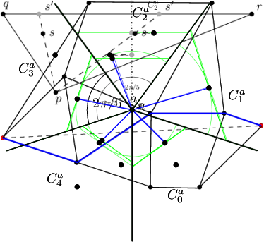
(a) Two examples for the position of $s$.

(b) The triangles $T_{ab}^{\ell}$ and $T_{ab}^{r}$.

Figure 3:

lemmaLemmaBaseCase Let $(a_{0},b_{0})$ be the pair of points in $P$ that minimizes $|ab|$ over all points $a$ and $b$ in $P$. The $\Theta_{5}$-graph of $P$ contains the edge $a_{0}b_{0}$.

Proof.

(See Figure 3(b).) Assume by contradiction that $\Theta_{5}$ does not contain $ab$, then some point $p\in P$ different from $a$ or $b$ is contained in $T_{ab}$. We show that $|bp|<|ab|$, hence $ab$ is not the closest pair in $P$.

Divide $T_{ab}$ into two triangles by separating $T_{ab}$ along $ab$ into the left triangle $T_{ab}^{\ell}$ and the right triangle $T_{ab}^{r}$. Then $p$ belongs to one of these triangles. Observation 1 gives us that $0\leq\alpha\leq\pi/10$, and thus $|ba|\geq|b\ell|\geq|br|$ and in both cases we can apply Lemma 1.∎

If $ab\in\Theta_{5}$, then $|\mathcal{P}(a,b)|\leq K|ab|$ holds for all $K\geq 1$. Otherwise we assume the following induction hypothesis: for every pair of points $a^{\prime},b^{\prime}\in P$ where $|a^{\prime}b^{\prime}|<|ab|$, the shortest path $\mathcal{P}(a^{\prime},b^{\prime})$ from $a^{\prime}$ to $b^{\prime}$ has length at most $|\mathcal{P}(a^{\prime},b^{\prime})|\leq K\cdot|a^{\prime}b^{\prime}|$, for some $K\geq 1$. Our goal is to find the minimum value of $K$ for which our inductive argument holds.

Recall that $c$ is the closest point to $a$ in $C_{2}^{a}$ and $d$ is the closest point to $b$ in $C_{4}^{b}$. We restrict our analysis to the following three paths:

1. $ac+\mathcal{P}(c,b)$,

2. $bd+\mathcal{P}(d,a)$, and

3. $ac+\mathcal{P}(c,d)+db$.

Depending on the particular arrangement of $a$, $b$, $c$, and $d$, we examine a subset of these and find a minimum value for $K$ that satisfies at least one of the following inequalities:

1. $|ac|+K\cdot|cb|\leq K\cdot|ab|$,

2. $|bd|+K\cdot|da|\leq K\cdot|ab|$, and

3. $|ac|+K\cdot|cd|+|db|\leq K\cdot|ab|$.

Observe that our inductive argument follows if any of these cases holds. For instance, if we prove A holds for some value $K$, it implies that $|cb|<|ab|$ (since all distances are positive), and thus $|\mathcal{P}(c,b)|\leq K\cdot|cb|$ by the induction hypothesis. Similar conclusions follow for statements B and C. Thus we can combine 1-3 with A-C as follows.

1. $|\mathcal{P}(a,b)|\leq|ac|+|\mathcal{P}(c,b)|\leq|ac|+K\cdot|cb|\leq K\cdot|ab|$.

2. $|\mathcal{P}(a,b)|\leq|bd|+|\mathcal{P}(d,a)|\leq|bd|+K\cdot|da|\leq K\cdot|ab|$.

3. $|\mathcal{P}(a,b)|\leq|ac|+|\mathcal{P}(c,d)|+|db|\leq|ac|+K\cdot|cd|+|db|\leq K\cdot|ab|$.

For any given arrangement of vertices we prove that at least one of A, B, or C holds true for some value $K$, and find the smallest value for which this is true. Our proof relies mainly on case analysis, but some of these cases have similar structure. We exploit this structure in Section 3 by designing two geometric lemmas that we apply repeatedly in the inductive step. These lemmas, along with additional arguments, are then applied to different arrangements of $a$, $b$, $c$, and $d$. For all but one case we show that at least one of a, b, or c holds true for $K\geq 5.70$. The last case requires $K\geq 6.16$. We improve this further to $K\geq 5.70$, but due to the complexity of this last case, we dedicate Section 4 to its analysis.

3 Analysis

We first introduce two triangles $T_{\ref{t253}}$ and $T_{\ref{t334}}$ for which inequalities of the form of A and B hold for reasonable values of $K$ (see Figure 4). Note the triangles are numbered to correspond to the lemmas they appear in. We state these inequalities as lemmas whose repeated use simplifies the proof of our main result.

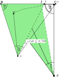
(a) $T_{\ref{t253}}$ has angles $(\frac{\pi}{5},\frac{\pi}{2},\frac{3\pi}{10})$.

(b) $T_{\ref{t334}}$ has angles $(\frac{3\pi}{10},\frac{3\pi}{10},\frac{2\pi}{5})$.

Figure 4: Triangles $T_{\ref{t253}}$ and $T_{\ref{t334}}$.

lemmaLemmaTRight (Figure 4(a)) Let $T_{\ref{t253}}$ be a triangle with vertices $(s,v,u)$ and corresponding interior angles $(\frac{\pi}{5},\frac{\pi}{2},\frac{3\pi}{10})$. Let $t$ be a point on $uv$ and let $w$ be a point inside $\triangle stu$. Then $|sw|+K|wt|\leq K|st|$ for all $K\geq 4.53$.

Proof.

(Figure 5(a)) We show $\Phi=|{s}{w}|+K|{w}{t}|-K|{s}{t}|\leq 0$. Without loss of generality, orient $T_{\ref{t253}}$ so that $u$ and $v$ define a horizontal line with $u$ left of $v$ and with $s$ below that line. Let ${w}_{r}$ be the horizontal projection of ${w}$ onto ${s}{t}$, and let ${w}_{\ell}$ be the horizontal projection of ${w}$ onto ${s}{u}$. We have $|{w}{w}_{r}|+|{w}_{r}{t}|\geq|{w}{t}|$ by the triangle inequality. We also have that $\angle{s}{w}{w}_{\ell}\geq\pi/2$, which implies that ${s}{w}_{\ell}$ is the longest edge in triangle ${s}{w}{w}_{\ell}$ (the triangle can be drawn inside a disk whose diameter is $sw_{\ell}$), and thus $|{s}{w}_{\ell}|\geq|{s}{w}|$. Since ${w}$ is on ${w}_{\ell}{w}_{r}$, we have $|{w}_{\ell}{w}_{r}|\geq|{w}{w}_{r}|$. Thus

$$\Phi =|{s}{w}|+K|{w}{t}|-K|{s}{t}|$$

$$\leq|{s}{w}_{\ell}|+K(|{w}{w}_{r}|+|{w}_{r}{t}|)-K(|{s}{w}_{r}|+|{w}_{r}{t}|)$$

$$\leq|{s}{w}_{\ell}|+K|{w}_{\ell}{w}_{r}|-K|{s}{w}_{r}|=\Phi^{\prime}.$$

Let $\beta=\angle vst\geq 0$. Observe that $\Phi^{\prime}$ increases as $\beta$ decreases, since $|{s}{w}_{r}|$ decreases while $|{w}_{\ell}{w}_{r}|$ increases and $|{s}{w}_{\ell}|$ stays constant. Hence, $\Phi^{\prime}$ is maximized when $\beta=0$, that is, when ${w}_{r}$ lies on ${s}{v}$. Thus assume that ${w}_{r}$ lies on ${s}{v}$ and let $|{s}{w}_{\ell}|=1$ without loss of generality. We bound $\Phi^{\prime}$ in terms of $\angle w_{r}sw_{\ell}=\frac{\pi}{5}$:

$$\Phi^{\prime}\leq 1+K\sin\left(\frac{\pi}{5}\right)-K\cos\left(\frac{\pi}{5}\right).$$

Solving for $K$ we get $\Phi\leq\Phi^{\prime}\leq 0$ when

$$K\geq\frac{1}{\cos(\frac{\pi}{5})-\sin(\frac{\pi}{5})}=4.52\ldots$$

∎

(a) $T_{\ref{t253}}$ has angles $(\frac{\pi}{5},\frac{\pi}{2},\frac{3\pi}{10})$.

(b) $T_{\ref{t334}}$ has angles $(\frac{3\pi}{10},\frac{3\pi}{10},\frac{2\pi}{5})$.

Figure 5: Detailed analysis of triangles $T_{\ref{t253}}$ and $T_{\ref{t334}}$.

lemmaLemmaTCone (Figure 4(b)) Let $T_{\ref{t334}}$ be a triangle with vertices $(s,v,u)$ and corresponding interior angles $(\frac{3\pi}{10},\frac{3\pi}{10},\frac{2\pi}{5})$. Let $t$ be a point on $uv$ such that $\angle vst\leq\pi/10$ and let $w$ be a point inside $\triangle stu$. Then $|sw|+K|wt|\leq K|st|$ for all $K\geq 5.70$.

Proof.

(Figure 5(b)) We show $\Phi=|{s}{w}|+K|{w}{t}|-K|{s}{t}|\leq 0$ by case analysis.

Case 1) $\angle vsw\leq\frac{\pi}{5}$ (Figure 6(a)): Let $v^{\prime}$ be the orthogonal projection of ${t}$ onto ${s}{v}$. Let ${u}^{\prime}$ be the point on the line through ${t}$ and $v^{\prime}$ such that $\angle v^{\prime}{s}{u}^{\prime}=\frac{\pi}{5}$. Observe that $\triangle sv^{\prime}u^{\prime}$ corresponds to $T_{\ref{t253}}$ of Lemma 4 and it contains ${w}$. Thus Lemma 4 tells us $\Phi\leq 0$ for all $K\geq 4.53$.

Case 2) $\angle vsw>\frac{\pi}{5}$ (Figure 6(b)): Without loss of generality, orient $T_{\ref{t334}}$ so that $u$ and $v$ define a horizontal line with $u$ left of $v$ and with $s$ below that line. Let ${w}_{r}$ be the horizontal projection of ${w}$ onto ${s}{t}$, and let ${w}_{\ell}$ be the horizontal projection of ${w}$ onto ${s}{u}$. We have $|{w}{w}_{r}|+|{w}_{r}{t}|\geq|{w}{t}|$ by the triangle inequality. We also have that $\angle{s}{w}{w}_{\ell}>\pi/2$, which implies that ${s}{w}_{\ell}$ is the longest edge in $\triangle{s}{w}{w}_{\ell}$ (the triangle can be drawn inside a disk whose diameter is $sw_{\ell}$), and thus $|{s}{w}_{\ell}|\geq|{s}{w}|$. Since ${w}$ is on ${w}_{\ell}{w}_{r}$, we have $|{w}_{\ell}{w}_{r}|\geq|{w}{w}_{r}|$. Thus

$$\Phi =|{s}{w}|+K|{w}{t}|-K|{s}{t}|$$

$$\leq|{s}{w}_{\ell}|+K(|{w}{w}_{r}|+|{w}_{r}{t}|)-K(|{s}{w}_{r}|+|{w}_{r}{t}|)$$

$$\leq|{s}{w}_{\ell}|+K|{w}_{\ell}{w}_{r}|-K|{s}{w}_{r}|=\Phi^{\prime}.$$

We rewrite $\Phi^{\prime}$ in terms of $\beta=\angle vst\geq 0$ using the sine law we get

$$|{s}{w}_{\ell}|=\frac{|{s}{w}_{r}|\sin\left(\frac{3\pi}{10}+\beta\right)}{\sin\left(\frac{2\pi}{5}\right)}$$

and

$$|{w}_{\ell}{w}_{r}|=\frac{|{s}{w}_{r}|\sin\left(\frac{3\pi}{10}-\beta\right)}{\sin\left(\frac{2\pi}{5}\right)}.$$

We normalize $\Phi^{\prime}$ by dividing each term by $\frac{|{s}{w}_{r}|}{\sin\left(\frac{2\pi}{5}\right)}$ which gives us

$$\Phi^{\prime}=\sin\left(\frac{3\pi}{10}+\beta\right)+K\sin\left(\frac{3\pi}{10}-\beta\right)-K\sin\left(\frac{2\pi}{5}\right).$$

The derivative of $\Phi^{\prime}$ with respect to $\beta$ is

$$\frac{d\Phi^{\prime}}{d\beta}=\cos\left(\frac{3\pi}{10}+\beta\right)-K\cos\left(\frac{3\pi}{10}-\beta\right).$$

For all $K\geq 1$, $\frac{d\Phi^{\prime}}{d\beta}(0)$ is negative and $\frac{d\Phi^{\prime}}{d\beta}(\beta)$ is monotone decreasing for $0\leq\beta\leq\frac{\pi}{10}$. Hence $\frac{d\Phi^{\prime}}{d\beta}$ is negative on the whole range $(K\geq 1)\times(0\leq\beta\leq\frac{\pi}{10})$ and $\Phi^{\prime}$ is maximized at $\beta=0$ for all $K\geq 1$. Thus

$$\Phi^{\prime}\leq\Phi^{\prime}(0)=\sin\left(\frac{3\pi}{10}\right)+K\sin\left(\frac{3\pi}{10}\right)-K\sin\left(\frac{2\pi}{5}\right).$$

Solving for $K$ we get $\Phi\leq\Phi^{\prime}\leq 0$ when

$$K\geq\frac{\sin\left(\frac{3\pi}{10}\right)}{\sin\left(\frac{2\pi}{5}\right)-\sin\left(\frac{3\pi}{10}\right)}=5.69\ldots$$

∎

(a) Using $T_{\ref{t253}}$ to analyze $T_{\ref{t334}}$.

(b) Proving $|{s}{w}_{\ell}|+K|{w}_{\ell}{w}_{r}|\leq K|{s}{w}_{r}|$

Figure 6: Analyzing triangle $T_{\ref{t334}}$.

As in the definition of $T_{ab}$ and $T_{ba}$ in Section 2, let $c$ be the point closest to $a$ in $T_{ab}$ and let $d$ be the point closest to $b$ in $T_{ba}$. We proceed by case analysis depending on the location of the points $c$ and $d$.

If $c$ is to the right of $ab$ or if $d$ is to the right of $ab$, we can apply Lemma 4 to show the existence of a short path from $a$ to $b$. When both $c$ and $d$ are left of $ab$, we use a more complicated argument requiring a new definition:

Definition 1.

(Figure 7) Given any pair of points $(a,b)$ in $P$, let $r^{\prime}$ and $r^{\prime}_{m}$ be as in the definition of $T_{ba}$ in Section 2. We define $P_{ab}$ to be the regular pentagon with vertices $(p_{0},p_{1},p_{2}=r^{\prime},p_{3}=r^{\prime}_{m},p_{4})$ where $p_{4}$ is above the line going through $r^{\prime}$ and $r^{\prime}_{m}$ (this uniquely defines the remaining points $p_{0}$ and $p_{1}$).

(a) $P_{ab}$ when $\alpha=0$.

(b) $P_{ab}$ when $\alpha=\pi/10$.

Figure 7: The regular pentagon $P_{ab}$.

Observe that $P_{ab}$ is fixed with respect to $T_{ba}$. This construction puts $p_{4}$ inside $T_{ab}$ and puts $p_{0}$ and $p_{1}$ on a horizontal line with $b$, with $p_{0}$ lying on the boundary of $T_{ab}$.

claimClaimPentagon Given Definition 1 we have that $p_{4}\in T_{ab}$, $p_{0}\in\ell b$, and $p_{1}$ lies on the line through $\ell$ and $b$.

Figure 8: Transformation 1.

Proof.

Note that $p_{3}p_{4}$ and $p_{3}b$ share the same supporting line since $\angle p_{2}p_{3}p_{4}=\angle p_{2}p_{3}b=\frac{3\pi}{5}$. Let $f$ be the intersection of $a\ell$ and $p_{3}b$. Given this observation and this definition, it is equivalent to prove that $p_{4}$ lies in the segment $fb$.

Translate $a$ on the segment $\ell^{\prime}_{m}\ell^{\prime}$. Since the slope of $a\ell$ is smaller than the slope of $\ell^{\prime}_{m}\ell^{\prime}$, translating $a$ to $a=\ell^{\prime}$, that is letting $\alpha=0$, maximizes the $y$-intercept of the line going through $a$ and $\ell$ with any fixed vertical line. Hence this translation shrinks $fb$, and it remains to prove that $p_{4}$ stays in $fb$ only in that extreme case.

With the simplifying assumption that $\alpha=0$, we show that $|p_{3}f|<|p_{3}p_{4}|<|p_{3}b|$, which proves the claim. Note that $\angle\ell ap_{3}=\pi/10$ and $\angle p_{3}fa=\pi/2$, thus $|p_{3}f|=|p_{3}a|\sin(\pi/10)$. We have $|p_{3}p_{4}|=|p_{3}p_{2}|=|p_{3}a|\sin{(\frac{\pi}{10}})/\sin{(\frac{3\pi}{10})}$. Since $|p_{3}a|=|p_{3}b|$, we obtain

$$|p_{3}b|\sin{\left(\frac{\pi}{10}\right)}<|p_{3}b|\frac{\sin{(\frac{\pi}{10}})}{\sin{(\frac{3\pi}{10})}}<|p_{3}b|.$$

∎

Given this definition, we consider the following cases: When $c$ is not in $P_{ab}$ we prove $|ac|+|\mathcal{P}(c,b)|\leq 5.70|ab|$. When $d$ is not in $P_{ab}$ we prove $|bd|+|\mathcal{P}(d,a)|\leq 5.70|ab|$. When both $c$ and $d$ are in $P_{ab}$ we analyze the length of the path $ac+\mathcal{P}(c,d)+db$. Lemma 9 gives us a bound of $6.16|ab|$ with a simple proof. Using a more technical analysis, we obtain a bound of $5.70|ab|$. This is proven in Lemma 10 in Section 4.

Some of the proofs use the simplifying assumption that $\alpha=\pi/10$. This is achieved through the following transformation: given $a$, $b$, $c$, $d\in P$ with $T_{ab}$ and $T_{ba}$ as defined earlier, we define:

Transformation 1.

Fix $b$, $c$, $d$, and $T_{ba}$, and translate $a$ along $r^{\prime}\ell^{\prime}$ until $a=\ell^{\prime}m$.

See Fig. 8. Observe that this transformation changes $|ac|$ and $|ab|$, but not $|bd|$, $|cd|$, or $|cb|$. The transformation also changes $|ad|$, but we do not use it in any case that depends on this value. We prove the following lemma allowing the application of Transformation 1 without loss of generality in several cases.

lemmaLemmaTransformation Under Transformation 1, the values of $|bd|$, $|cd|$, and $|cb|$ are unchanged, and $\Psi=|ac|-K|ab|$ is maximized when $a=\ell_{m}^{\prime}$ for all $K\geq 3.24$.

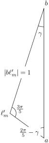
Figure 9: The values used in the proof of Lemma 1.

Proof.

(Figure 9) Let $\gamma=\angle\ell_{m}^{\prime}ba=\pi/10-\alpha$. Define $\Psi^{\prime}=|a\ell_{m}^{\prime}|+|\ell_{m}^{\prime}c|-K|ab|.$ Note by the triangle inequality that $\Psi^{\prime}\geq\Psi$. We show that $\Psi^{\prime}$ is monotonically decreasing in $\gamma$, which proves both $\Psi$ and $\Psi^{\prime}$ are maximized when $\gamma=0$ since then $\Psi=\Psi^{\prime}$. We let $|b\ell_{m}^{\prime}|=1$ without loss of generality and express $\Psi^{\prime}$ as a function of $\gamma$ using the law of sines:

Using $|a\ell_{m}^{\prime}|=\frac{\sin{\gamma}}{\sin{(\frac{2\pi}{5}-\gamma)}}$ and $|ab|=\frac{\sin{(\frac{3\pi}{5})}}{\sin{(\frac{2\pi}{5}-\gamma)}}=\frac{\sin{(\frac{2\pi}{5})}}{\sin{(\frac{2\pi}{5}-\gamma)}}$, we have

$$\Psi^{\prime}=\frac{\sin{\gamma}-K\sin{(\frac{2\pi}{5})}}{\sin{(\frac{2\pi}{5}-\gamma)}}+\underbrace{|\ell_{m}^{\prime}c|}_{\text{Independent of }\gamma}.$$

Hence,

$$\frac{d\Psi^{\prime}}{d\gamma} =\frac{\cos\gamma\sin(\frac{2\pi}{5}-\gamma)+\cos(\frac{2\pi}{5}-\gamma)(\sin\gamma-K\sin(\frac{2\pi}{5}))}{\sin^{2}(\frac{2\pi}{5}-\gamma)}$$

$$=\frac{\sin(\frac{2\pi}{5})(1-K\cos(\frac{2\pi}{5}-\gamma))}{\sin^{2}(\frac{2\pi}{5}-\gamma)}.$$

Since $0\leq\gamma\leq\pi/10$, the denominator is positive on the whole range and the numerator is maximized when $\gamma=0$. Since $\sin(\frac{2\pi}{5})$ is positive, it suffices to satisfy $1-K\cos(\frac{2\pi}{5})\leq 0$:

$$K\geq\frac{1}{\cos{(\frac{2\pi}{5})}}=3.23\ldots$$

∎

By Lemma 1 we see that by applying Transformation 1 we maximize the value $|ac|-K|ab|$. Another way to see this is that we minimize $K|ab|$. This, in turn, allows us to explicitly determine under what conditions the inductive hypothesis applies. Note that applying Transformation 1 to where $a=\ell_{m}^{\prime}$ is equivalent to assuming $\alpha=\pi/10$.

All these proofs can be combined in an analysis comprising eight cases depending on the location of $c$ and $d$ with respect to $T_{ab}$, $T_{ba}$, and $P_{ab}$, as illustrated below in the breakdown of the case analysis below. In each case we prove that for a given arrangement of vertices that $|\mathcal{P}(a,b)|\leq K|ab|$ for the given value $K$.

1. If $c$ is right of $ab$, then $K\geq 4.53$ by Lemma 2.

2. If $d$ is right of $ab$, then $K\geq 4.53$ by Lemma 3.

3. Else both $c$ and $d$ are left of $ab$. We have the following cases:

   1. If $c$ is in $T_{ba}$, then $K\geq 5.70$ by Lemma 4.

   2. Else $c$ is NOT in $T_{ba}$ and:

      1. If $c$ is NOT in $P_{ab}$ then $K\geq 4.53$ by Lemma 5.

      2. Else $c$ is in $P_{ab}$ and:

         • If $d$ is right of $am$ then $K\geq 3.24$ by Lemma 6.

         • If $d$ is left of $am$ and above $c$ then $K\geq 4.53$ by Lemma 7

         • If $d$ is left of $am$ and below $c$ (i.e. $d\not\in T_{ab}$ such that $bd$ and $ac$ cross)

           • If $d$ is NOT in $P_{ab}$ then $K\geq 5.70$ by Lemma 8.

           • If $d$ is in $P_{ab}$ then $K\geq 6.16$ by Lemma 9 or $K\geq 5.70$ by Lemma 10.

Breakdown of the case analysis 1

One can check that all locations of $c$ and $d$ are covered. This proves our main theorem: theoremTheoremMain Given a set $P$ of points in the plane, the $\Theta_{5}$-graph of $P$ is a $5.70$-spanner.

We use the remainder of the paper to prove each lemma.

Figure 10: Points $(a,r,m)$ correspond to $T_{\ref{t253}}$ (in blue) with ${t}=b$ and ${w}=c$.

Figure 11: Points $(b,m^{\prime},\ell^{\prime})$ correspond to $T_{\ref{t253}}$ (in blue) with ${t}=a$ and ${w}=d$.

Lemma 2.

If $c$ is right of $ab$, then $|\mathcal{P}(a,b)|\leq K|ab|$ for $K\geq 4.53$.

Proof.

(Figures 4, 11) Let $({s},{t},{w},{u},{v})=(a,b,c,r,m)$, thus these points correspond to triangle $T_{\ref{t253}}$ of Lemma 4. Thus $|ac|+K|cb|\leq K|ab|$ for all $K\geq 4.53$. The induction hypothesis and Lemma 4 imply that there is a path from $a$ to $b$ with length at most

$$|\mathcal{P}(a,b)|\leq|ac|+|\mathcal{P}(c,b)|\leq|ac|+K|cb|\leq K|ab|.$$

∎

Lemma 3.

If $d$ is right of $ab$, then $|\mathcal{P}(a,b)|\leq K|ab|$ for $K\geq 4.53$.

Proof.

(Figures 4, 11) Let $({s},{t},{w},{u},{v})=(b,a,d,m^{\prime},\ell^{\prime})$, thus these points correspond to triangle $T_{\ref{t253}}$ from Lemma 4. Thus $|bd|+K|da|\leq K|ab|$ for $K\geq 4.53$ by Lemma 4. The induction hypothesis and Lemma 4 imply that there is a path from $a$ to $b$ with length at most

$$|\mathcal{P}(a,b)|\leq|bd|+|\mathcal{P}(d,a)|\leq|bd|+K|da|\leq K|ab|.$$

∎

Lemma 4.

If $c$ is left of $ab$ and in $T_{ab}\cap T_{ba}$, then $|\mathcal{P}(a,b)|\leq K|ab|$ for $K\geq 5.70$.

Figure 12: Points $(a,q,p)$ correspond to the triangle $T_{\ref{t334}}$ with angles $(\frac{3\pi}{10},\frac{2\pi}{5},\frac{3\pi}{10})$ as denoted by the blue triangle. Let ${t}=b$ and ${w}=c$, and $\theta=\frac{\pi}{10}-\alpha$, which falls in the range of $0\leq\angle{v}{s}{u}\leq\pi/10$.

Figure 13: We use the fact that $p_{4}$ lies in $T_{ab}$ and apply $T_{\ref{t334}}$.

Proof.

(Figures 4, 13) Let $p$ be the intersection of $br^{\prime}$ and $a\ell$, and let $q$ be the intersection of the lines through $r^{\prime}b$ and $ar_{m}$. Observe that $0\leq\angle r_{m}ab\leq\pi/10$, thus $\angle r_{m}ab$ has the same range as $\angle{v}{s}{t}$ from $T_{\ref{t334}}$ in Lemma 5. If we let points $({s},{t},{w},{u},{v})=(a,b,c,p,q)$, then these points correspond to the triangle $T_{\ref{t334}}$, and thus $|ac|+K|cb|\leq K|ab|$ for $K\geq 5.70$ by Lemma 5. Our induction hypothesis and Lemma 5 imply that there is a path from $a$ to $b$ with length

$$|\mathcal{P}(a,b)|\leq|ac|+|\mathcal{P}(c,b)|\leq|ac|+K|cb|\leq K|ab|.$$

∎

Lemma 5.

If $c\in T_{ab}\setminus(T_{ba}\cup P_{ab})$, then $|\mathcal{P}(a,b)|\leq K|ab|$ for all $K\geq 4.53$.

Proof.

(Figures 4, 7(b)) Let $\Phi=|ac|+K|cb|-K|ab|$. We apply Transformation 1. Since $c\not\in T_{ba}$ it must be left of $\ell_{m}^{\prime}b$, thus $c$ remains left of $ab$. As $a$ moves left along $\ell^{\prime}\ell^{\prime}_{m}$, so does the left side of $T_{ab}$, which means that $c$ remains inside $T_{ab}$. Thus Lemma 1 implies that $\Phi$ is maximized at $\alpha=\pi/10$, thus we assume this is the case. Observe that $\angle ba\ell_{m}=\pi/5$, and $\angle\ell_{m}ba=2\pi/5<\pi/2$. Let $q$ be the intersection of the line through $b$ orthogonal to $ab$ and the line through $a$ and $\ell_{m}$. If we let $({s},{t},{w},{u},{v})=(a,b,c,q,b)$ then these points correspond to $T_{\ref{t253}}$. Then Lemma 4 tells us that $|ac|+K|cb|\leq K|ab|$ and thus $\Phi=|ac|+K|cb|-K|ab|\leq 0$ for all $K\geq 4.53$. ∎

Figure 14: The point $c$ is in $P_{ab}\setminus T_{ba}$, and $d$ is right of $am$.

Figure 15: The segments $ac$ and $bd$ cross and $c$ and $d$ are in $P_{ab}$.

Lemma 6.

If $d$ is left of $ab$ and right of $am$, then $|\mathcal{P}(a,b)|\leq K|ab|$ for $K\geq 3.24$.

Proof.

(Figure 15) We show $\Phi=|bd|+K|da|-K|ab|\leq 0$, which implies $|\mathcal{P}(a,b)|\leq|bd|+|\mathcal{P}(d,a)|\leq K|ab|$ by the triangle inequality and the induction hypothesis.

Let $d^{\prime}$ be the horizontal projection of $d$ onto $ab$. Let $\Phi_{1}=|bd|-K|bd^{\prime}|$ and $\Phi_{2}=K|da|-K|d^{\prime}a|$, and note that $\Phi=\Phi_{1}+\Phi_{2}$ since $d^{\prime}\in ab$. Thus it is sufficient to show that $\Phi_{1}\leq 0$ and $\Phi_{2}\leq 0$.

Observe that $\angle d^{\prime}da>\pi/2$, since $d$ is right of $am$, thus $|d^{\prime}a|>|da|$, and $\Phi_{2}\leq 0$ for all $K\geq 1$. For $\Phi_{1}\leq 0$ we need $K\geq\frac{|bd|}{|bd^{\prime}|}$. Let $\gamma=\angle d^{\prime}db$ and note that $\gamma\geq\pi/10$ because $d\in T_{ba}$. Let $d_{y}(b,d^{\prime})$ be the vertical distance between $b$ and $d^{\prime}$. We have $\sin\gamma=\frac{d_{y}(b,d^{\prime})}{|bd|}$. Observe that $d_{y}(b,d^{\prime})\leq|bd^{\prime}|$ and thus $\frac{|bd|}{|bd^{\prime}|}\leq\frac{|bd|}{d_{y}(b,d^{\prime})}=\frac{1}{\sin\gamma}\leq\frac{1}{\sin(\pi/10)}$. Thus $K\geq\frac{1}{\sin(\pi/10)}\geq\frac{|bd|}{d_{y}(b,d^{\prime})}$, and $K\geq\frac{1}{\sin(\pi/10)}=3.23\dots$ is sufficient. ∎

(a) We have $|db|-K|bd^{\prime}|\leq 0$.

(b) We have $|ac|+K|cd|-K|ad^{\prime}|\leq 0$.

Figure 16: The point $c$ is in $P_{ab}\setminus T_{ba}$, and $d$ is left of $am$ but above $c$.

Lemma 7.

If $c$ is in $P_{ab}\setminus T_{ba}$, and $d$ is left of $am$ but above $c$, then $|\mathcal{P}(a,b)|\leq K|ab|$ for all $K\geq 4.53$.

Proof.

(Figures 4, 16) We show $\Phi=|ac|+K|cd|+|db|-K|ab|\leq 0$, which implies $|\mathcal{P}(a,b)|\leq|ac|+|\mathcal{P}(c,d)|+|db|\leq K|ab|$ by the triangle inequality and the induction hypothesis. We split $\Phi$ into two parts, and show that each part is less than $0$. Let $d^{\prime}$ be the horizontal projection of $d$ onto $ab$. Let $\Phi_{1}=|bd|-K|bd^{\prime}|$, and let $\Phi_{2}=|ac|+K|cd|-K|ad^{\prime}|$. Observe that $\Phi=\Phi_{1}+\Phi_{2}$ since $d^{\prime}\in ab$.

To show that $\Phi_{1}\leq 0$, observe that $d_{y}(b,d)=d_{y}(b,d^{\prime})\leq|bd^{\prime}|$. Thus let $\Phi_{1}^{\prime}=|bd|-K\cdot d_{y}(b,d)\geq\Phi_{1}$. Let $\gamma=\angle d^{\prime}db$, and observe that $\Phi_{1}^{\prime}=|bd|(1-K\sin\gamma)$. Note that $\gamma\geq\pi/10$ since $d\in T_{ba}$, and thus $K\geq 3.24$ is sufficient to have $\Phi_{1}\leq 0$.

For $\Phi_{2}\leq 0$, let $d^{\prime\prime}$ be the horizontal projection of $d$ onto $am$. Since $\angle ad^{\prime\prime}d^{\prime}=\pi/2$, $|ad^{\prime\prime}|\leq|ad^{\prime}|$. Since $c\not\in T_{ba}$, $\angle cdd^{\prime\prime}\geq 9\pi/10$, thus $|cd^{\prime\prime}|>|cd|$. Let $\Phi_{2}^{\prime}=|ac|+K|cd^{\prime\prime}|-K|ad^{\prime\prime}|\geq\Phi_{2}$. Let $q$ be the horizontal projection of $d^{\prime\prime}$ onto $a\ell$. Let the points $({s},{t},{w},{u},{v})=(a,d^{\prime\prime},c,q,d^{\prime\prime})$ and thus these points correspond to $T_{\ref{t253}}$. Thus $|ac|+K|cd^{\prime\prime}|\leq K|ad^{\prime\prime}|$ for all $K\geq 4.53$ by Lemma 4. ∎

Lemma 8.

If $d$ is left of $ab$, below $c$ and not in $P_{ab}$, then $|\mathcal{P}(a,b)|\leq K|ab|$ for all $K\geq 5.70$.

Proof.

(Figures 4, 13) We note that $ac$ and $bd$ intersect and $d$ must be outside of $T_{ab}$ (otherwise $ad$ would be and edge of $\Theta_{5}$, but not $ac$). We first show that $d$ is below $br_{m}^{\prime}$. Recall that $P_{ab}$ is fixed with respect to $T_{ba}$. Since $d$ is outside of $T_{ab}$ and $P_{ab}$, if $p_{4}p_{0}$ is inside $T_{ab}$, $d$ must be below $br_{m}^{\prime}$. Since the slope of $p_{0}p_{4}$ is less than the slope of $\ell a$, it is sufficient to show that $p_{4}$ is inside $T_{ab}$ which follows by Claim 7. By Observation 1 we have that $0\leq\angle ab\ell^{\prime}\leq\pi/10$. Thus we can map the points $({s},{t},{w},{u},{v})$ to $(b,a,d,r_{m}^{\prime},\ell^{\prime})$ and apply Lemma 5. Thus $|bd|+K|da|\leq K|ab|$ for $K\geq 5.70$. Our induction hypothesis and Lemma 5 imply that there is a path from $b$ to $a$ with length at most

$$|\mathcal{P}(a,b)|\leq|bd|+|\mathcal{P}(d,a)|\leq|bd|+K|da|\leq K|ab|.$$

∎

Lemma 9.

If $ac$ and $bd$ cross and both $c$ and $d$ are in $P_{ab}$, then $|\mathcal{P}(a,b)|\leq K|ab|$ for $K\geq 6.16$.

Proof.

(Figures 4, 15) We show $\Phi=|ac|+K|cd|+|db|-K|ab|\leq 0$, which implies $|\mathcal{P}(a,b)|\leq|ac|+|\mathcal{P}(c,d)|+|db|\leq K|ab|$ by the triangle inequality and the induction hypothesis. Under Transformation 1, Lemma 1 implies that $\Phi$ is maximized when $\alpha=\pi/10$, so we assume this is the case. Since $c$, $d$, and $P_{ab}$ are fixed, $c$ and $d$ are still inside $P_{ab}$ after Transformation 1. Given that $c$ and $d$ are in $P_{ab}$, the furthest apart $c$ and $d$ can be is if they are both on a diagonal of $P_{ab}$. The length of one side of $P_{ab}$ is at most $\frac{\sin(\pi/10)}{\sin(3\pi/10)}|ab|$. That means a diagonal of $P_{ab}$, and thus $|cd|$, has length at most $2\sin(3\pi/10)\frac{\sin(\pi/10)}{\sin(3\pi/10)}|ab|=2\sin(\pi/10)|ab|$. At their longest, $|ac|$ and $|bd|$ each have length $\frac{\sin(2\pi/5)}{\sin(3\pi/10)}|ab|$ by the law of sines. We want

$$\Phi=|ac|+K|cd|+|db|-K|ab|\leq 0.$$

Solving for $K$ gives

$$K\geq\frac{|ac|+|db|}{|ab|-|cd|}\geq\frac{2\cdot\sin(2\pi/5)}{\sin(3\pi/10)\cdot(1-2\cdot\sin(\pi/10))}=6.15\ldots$$

∎

4 Proving a spanning ratio of $5.70$

In this section we present a lemma with a stronger bound for the case handled by Lemma 9. Proving this lemma requires a careful analysis of the locations of $c$ and $d$ and the tradeoffs between the values of $|ac|+|db|$ and $K|cd|$. Let $\Phi=|ac|+K|cd|+|db|-K|ab|$. For the rest of this section, assume we have applied Transformation 1, and thus $\alpha=\pi/10$ and $\Phi$ is maximized. Since $P_{ab}$, $c$ and $d$ are fixed, both $c$ and $d$ are still in $P_{ab}$. Let $c^{\prime}$ be the intersection of the line through $a$ and $c$ and the segment $p_{0}p_{1}$, and let $d^{\prime}$ be the intersection of the line through $b$ and $d$ and the segment $p_{3}p_{4}$. See Figure 17. Let $\Phi^{\prime}=|ac^{\prime}|+K|c^{\prime}d^{\prime}|+|d^{\prime}b|-K|ab|$, and let $\Phi^{\prime\prime}=|ap_{1}|+K|p_{1}p_{3}|+|p_{3}b|-K|ab|$.

Figure 17: Points $c^{\prime}$ and $d^{\prime}$.

We split the analysis into three steps that amount to proving the following lemmas: lemmaLemmaMainOne For all $K\geq 5.70$, $\Phi\leq\Phi^{\prime}$. lemmaLemmaMainTwo For all $K\geq 5.70$, $\Phi^{\prime}\leq\Phi^{\prime\prime}$. lemmaLemmaIntermediate For all $K\geq 5.70$, $\Phi^{\prime\prime}\leq 0$.

The following lemma follows from these lemmas, the triangle inequality, and the induction hypothesis. It supersedes Lemma 9:

Lemma 10.

If $ac$ and $bd$ intersect and both $c$ and $d$ are in $P_{ab}$, then $|\mathcal{P}(a,b)|\leq K|ab|$ for $K\geq 5.70$.

Substituting Lemma 10 for Lemma 9 in the proof of Theorem 1 brings the spanning ratio of the $\Theta_{5}$-graph down to $5.70$. We are left with proving Lemmas 17, 17, and 17, which is done in the next three subsections.

(a) Proof that $|c^{\prime}d|\geq|cd|$.

(b) Maximum of $\angle ed^{\prime}c^{\prime}$.

Figure 18: Finding the longest distance from $a$ to $b$ when $c$ and $d$ are in $P_{ab}$,

4.1 Proof of Lemma 17

Lemma 17 states that $|ac|+|bd|+K|cd|-K|ab|\leq|ac^{\prime}|+|bd^{\prime}|+K|c^{\prime}d^{\prime}|-K|ab|$ for $K\geq 5.70$. See Figure 18(a). Let $e$ be the intersection of $ac$ and $bd$, and let $e^{\prime}$ be the intersection of $br^{\prime}$ and $a\ell$. Observe that $\angle\ell e^{\prime}r^{\prime}=2\pi/5$, and thus we can see that $\angle dec\geq 2\pi/5$. This implies that $\angle dec$ cannot be the smallest angle in $\triangle dec$, since that would require $\angle dec\leq\pi/3$. Thus at least one of $\angle dce$ and $\angle edc$ is the smallest angle in $\triangle dec$. Since we have applied Transformation 1, and can thus assume that $\alpha=\pi/10$, the cases are symmetric. We can therefore, without loss of generality, assume that $\angle dce$ is the smallest angle in $\triangle dec$.

*

Proof.

Since $c$ lies on $ac^{\prime}$ and $d$ lies on $bd^{\prime}$, we have $|ac|\leq|ac^{\prime}|$ and $|bd|\leq|bd^{\prime}|$, and it is sufficient to show that $|cd|\leq|c^{\prime}d^{\prime}|$. We first show that $|cd|\leq|c^{\prime}d|$. Since $\angle dce$ is the smallest angle in $\triangle dec$, $\angle dce<\pi/3$. That implies that $\angle c^{\prime}cd>\pi/2$, which implies that $c^{\prime}d$ is the longest side of triangle $\triangle cc^{\prime}d$, and thus $|cd|\leq|c^{\prime}d|$. See Fig.18(a).

We now show that $|c^{\prime}d^{\prime}|\geq|c^{\prime}d|$. If $\angle c^{\prime}dd^{\prime}\geq\pi/2$, then $c^{\prime}d^{\prime}$ is the longest side of $\triangle c^{\prime}dd^{\prime}$, and $|c^{\prime}d^{\prime}|\geq|c^{\prime}d|$ and we are done. Otherwise assume $\angle c^{\prime}dd^{\prime}<\pi/2$.

The law of sines tells us that $\frac{|c^{\prime}d^{\prime}|}{\sin\angle c^{\prime}dd^{\prime}}=\frac{|c^{\prime}d|}{\sin\angle dd^{\prime}c^{\prime}}$. Since $\sin\theta$ is an increasing function for $0\leq\theta<\pi/2$, showing that $\angle c^{\prime}dd^{\prime}\geq\angle dd^{\prime}c^{\prime}$ is sufficient to show $|c^{\prime}d^{\prime}|\geq|c^{\prime}d|$, as it would imply both angles are $<\pi/2$. Observe that $\angle c^{\prime}dd^{\prime}\geq\angle c^{\prime}ed^{\prime}$ and $\angle ed^{\prime}c^{\prime}=\angle dd^{\prime}c^{\prime}$, thus it is sufficient to prove that $\angle c^{\prime}ed^{\prime}\geq\angle ed^{\prime}c^{\prime}$.

Observe that $\angle ced=\angle c^{\prime}ed^{\prime}\geq 2\pi/5$. We now find the maximum of $\angle dd^{\prime}c^{\prime}=\angle ed^{\prime}c^{\prime}\leq 2\pi/5$. Observe that if $c^{\prime}$ moves left, $\angle ed^{\prime}c^{\prime}$ increases, thus assume $c^{\prime}$ is at $p_{1}$. Let $O(bp_{3}c^{\prime})$ be the circle through $b$, $p_{3}$, and $c^{\prime}$ with center $o$. Observe that $o$ lies on $br^{\prime}$. Observe that $\angle r^{\prime}bd^{\prime}=\pi/10$, thus $\angle r^{\prime}op_{3}=\pi/5$. Segment $or^{\prime}$ makes an angle of $\pi/10$ with the horizontal line through $o$. Thus $od^{\prime}$ makes an angle of $3\pi/10$ with the horizontal line through $o$, and thus the line tangent to $O(bp_{3}c^{\prime})$ at $p_{3}$ is the line supporting $\ell^{\prime}r^{\prime}$, since $\ell^{\prime}r^{\prime}$ makes an angle of $3\pi/10$ with the vertical line through $\ell^{\prime}$. See Figure 18(b). That implies that $[p_{2},p_{3})$ lies outside of $O(bp_{3}c^{\prime})$, which means for every point $d^{\prime}$, $\angle ed^{\prime}c^{\prime}\leq\angle ep_{3}c^{\prime}=2\pi/5$, and thus $\angle c^{\prime}dd^{\prime}\geq\angle dd^{\prime}c^{\prime}$ as required. ∎

Figure 19: An example of $\Phi^{\prime\prime}$.

4.2 Proof of Lemma 17

Observe that $|ap_{1}|+K|p_{1}p_{3}|+|p_{3}b|=|ap_{0}|+K|p_{0}p_{2}|+|p_{2}b|$ when $\alpha=\pi/10$, since $T_{ab}$ and $T_{ba}$ are the same size and the cases are symmetric. We prove that

$$\Phi^{\prime}=|ac^{\prime}|+K|c^{\prime}d^{\prime}|+|d^{\prime}b|-K|ab| \leq|ap_{1}|+K|p_{1}p_{3}|+|p_{3}b|-K|ab|=\Phi^{\prime\prime}$$

$$=|ap_{0}|+K|p_{0}p_{2}|+|p_{2}b|-K|ab|.$$

(a) The point $q$ such that $|p_{1}q|=|c^{\prime}d^{\prime}|$ lies between $d^{\prime}$ and $p_{2}$.

(b) We look at the change in $|d^{\prime}p_{3}|+K|c^{\prime}d^{\prime}|$ with respect to $\theta$.

Figure 20:

*

Proof.

(Figure 19) Without loss of generality, we assume that $|p_{1}c^{\prime}|\leq|p_{2}d^{\prime}|$. We show that $\Phi^{\prime}$ is maximized when $c^{\prime}=p_{1}$ and $d^{\prime}=p_{3}$.

(Figure 20(a)) Observe that $|p_{1}p_{2}|\leq|c^{\prime}d^{\prime}|\leq|p_{1}p_{3}|$. Let $z$ be a point on $p_{2}p_{3}$ that moves from $p_{2}$ to $p_{3}$, and observe that $|p_{1}z|$ takes on every value from $|p_{1}p_{2}|$ to $|p_{2}p_{3}|$. Thus there must be a point $q$ on $p_{2}p_{3}$ such that $|p_{1}q|=|c^{\prime}d^{\prime}|$.

We claim that $|ap_{1}|+|bq|\geq|ac^{\prime}|+|bd^{\prime}|$, which implies that $\Phi^{\prime}\leq|ap_{1}|+K|p_{1}q|+|qb|-K|ab|$.

Observe $|ap_{1}|\geq|ac^{\prime}|$, since $\angle p_{1}c^{\prime}a>\pi/2$, making $ap_{1}$ the longest edge in triangle $\triangle ac^{\prime}p_{1}$. We claim that $q$ is between $d^{\prime}$ and $p_{2}$, and thus $|bq|\geq|bd^{\prime}|$ since $\angle bd^{\prime}q>\pi/2$. By contradiction, assume that $q$ is between $d^{\prime}$ and $p_{3}$. Since $|p_{1}c^{\prime}|\leq|p_{2}d^{\prime}|$, $\angle qd^{\prime}c^{\prime}>\pi/2$, which implies that $|c^{\prime}q|>|c^{\prime}d^{\prime}|$. Also note that $\angle qd^{\prime}p_{1}>\pi/2$, which implies $|p_{1}q|>|c^{\prime}q|>|c^{\prime}d^{\prime}|$, a contradiction. Thus assuming that $c^{\prime}=p_{1}$ and $d^{\prime}=q$ does not decrease $\Phi^{\prime}$.

Now, given that $c^{\prime}$ is on $p_{1}$, we show that $\Phi^{\prime}\leq|ac^{\prime}|+|bp_{3}|+K|c^{\prime}p_{3}|$, that is, when $d^{\prime}$ is on $p_{3}$. To do this we define another function $\Phi^{*}=|ac^{\prime}|+|d^{\prime}p_{3}|+|p_{3}b|+K|c^{\prime}d^{\prime}|-K|ab|$. See Figure 20(b). Since $|bd^{\prime}|\leq|d^{\prime}p_{3}|+|p_{3}b|$ by the triangle inequality, $\Phi^{\prime}\leq\Phi^{*}$, and observe that $\Phi^{\prime}=\Phi^{*}=\Phi^{\prime\prime}$ when $d^{\prime}=p_{3}$. We show that $\Phi^{*}$ is maximized when $d^{\prime}=p_{3}$, thus implying that $\Phi^{\prime}$ is also maximized when $d^{\prime}=p_{3}$, and $\Phi^{\prime}\leq\Phi^{\prime\prime}$. Let $\theta=\angle p_{2}p_{1}d^{\prime}$. We allow $d^{\prime}$ to move along $p_{2}p_{3}$ until $d^{\prime}$ is on $p_{3}$, and fix all other points, and observe how $\Phi^{*}$ changes with $\theta$.

We first rewrite $\Phi^{*}$ as $\Phi^{*}=|ac^{\prime}|+|p_{2}p_{3}|-|p_{2}d^{\prime}|+|p_{3}b|+K|c^{\prime}d^{\prime}|-K|ab|$. Using the sine law we get $|p_{2}d^{\prime}|=\frac{\sin\theta}{\sin(2\pi/5-\theta)}|p_{1}p_{2}|$, and $|c^{\prime}d^{\prime}|=\frac{\sin(3\pi/5)}{\sin(2\pi/5-\theta)}|p_{1}p_{2}|$. All other terms of $\Phi^{*}$ have fixed values with respect to $\theta$. Thus

$$\frac{d\Phi^{*}}{d\theta} =\frac{d}{d\theta}\left(K\frac{\sin(3\pi/5)}{\sin(2\pi/5-\theta)}|p_{1}p_{2}|-\frac{\sin\theta}{\sin(2\pi/5-\theta)}|p_{1}p_{2}|\right)$$

$$=\frac{K\cos(2\pi/5-\theta)\sin(3\pi/5)-\cos\theta\sin(2\pi/5-\theta)-\sin\theta\cos(2\pi/5-\theta)}{\sin^{2}(2\pi/5-\theta)}|p_{1}p_{2}|$$

$$=\frac{K\cos(2\pi/5-\theta)\sin(3\pi/5)-\sin(2\pi/5)}{\sin^{2}(2\pi/5-\theta)}|p_{1}p_{2}|.$$ (1)

Observe that $0\leq\theta\leq 3\pi/10$. The denominator of (1) is always positive. The numerator of (1) is minimized at $\theta=0$, which for $K\geq 5.70$ is positive. Thus (1) is always positive for $0\leq\theta\leq 3\pi/10$, thus $\Phi^{*}$ is increasing in $\theta$, and is maximized when $d^{\prime}=p_{3}$, as required. Thus $\Phi^{\prime}\leq\Phi^{*}\leq\Phi^{\prime\prime}=|ap_{1}|+K|p_{1}p_{3}|+|p_{3}b|-K|ab|$ as required. ∎

4.3 Proof of Lemma 17

*

Proof.

(Figure 19) We apply Transformation 1 with $\alpha=\frac{\pi}{10}$ and assume that $|ab|=1$. Then using the law of sines we get $|bp_{3}|=1$, $|ap_{1}|=\frac{\sin(2\pi/5)}{\sin(3\pi/10)}$, and $|p_{1}p_{3}|=2\sin(3\pi/10)\frac{\sin(\pi/10)}{\sin(3\pi/10)}=2\sin(\pi/10)$. We want

$$\Phi^{\prime\prime}=|ap_{1}|+K|p_{1}p_{3}|+|p_{3}b|-K|ab|\leq 0.$$

Solving for $K$ gives

$$K\geq\frac{|ap_{1}|+|p_{3}b|}{|ab|-|p_{1}p_{3}|}=\frac{\frac{\sin(2\pi/5)}{\sin(3\pi/10)}+1}{1-2\sin(\pi/10)}=5.69\ldots$$

∎

5 Open Problems

Using a few simple geometric observations and arguments, we have lowered the spanning ratio of $\Theta_{5}$ from $9.96$ to $5.70$, bringing us closer to the lower bound of $3.798$ and thus a tight bound. The obvious open problem that remains is closing the gap between the upper and lower bound on the spanning ratio of the $\Theta_{5}$-graph.

Acknowledgements:

We thank Elena Arseneva for many fruitful discussions on the topic.

References

[1]
O. Aichholzer, S. W. Bae, L. Barba, P. Bose, M. Korman, A. van Renssen,
P. Taslakian, and S. Verdonschot.
Theta-3 is connected.
Computational geometry, 47(9):910–917, 2014.
[2]
L. Barba, P. Bose, J. L. De Carufel, A. van Renssen, and S. Verdonschot.
On the stretch factor of the Theta-4 graph.
In Proceedings of the 13th International Symposium on Algorithms
and Data Structures (WADS), pages 109–120, 2013.
[3]
P. Bose, J. L. De Carufel, D. Hill, and M. Smid.
On the spanning and routing ratio of Theta-four.
In Proceedings of the Thirtieth Annual ACM-SIAM Symposium on
Discrete Algorithms (SODA), pages 2361–2370, 2019.
[4]
P. Bose, J. L. De Carufel, P. Morin, A. van Renssen, and S. Verdonschot.
Towards tight bounds on Theta-graphs: More is not always better.
Theoretical Computer Science, 616:70–93, 2016.
[5]
P. Bose, P. Morin, A. van Renssen, and S. Verdonschot.
The Theta-5-graph is a spanner.
Computational Geometry, 48(2):108–119, 2015.
[6]
L. P. Chew.
There are planar graphs almost as good as the complete graph.
Journal of Computer and System Sciences, 39(2):205 – 219,
1989.
[7]
K. Clarkson.
Approximation algorithms for shortest path motion planning.
In Proceedings of the Nineteenth Annual ACM Symposium on Theory
of Computing (STOC), pages 56–65, 1987.
[8]
J. M. Keil.
Approximating the complete Euclidean graph.
In Proceedings of the 1st Scandinavian Workshop on Algorithm
Theory (SWAT), pages 208–213, 1988.
[9]
J. M. Keil and C. A. Gutwin.
Classes of graphs which approximate the complete Euclidean graph.
Discrete & Computational Geometry, 7(1):13–28, 1992.
[10]
N. M. El Molla.
Yao spanners for wireless ad-hoc networks.
PhD thesis, Villanova University, 2009.
[11]
J. Ruppert and R. Seidel.
Approximating the d-dimensional complete Euclidean graph.
In Proceedings of the 3rd Canadian Conference on Computational
Geometry (CCCG), 1991.