Lower Perplexity is Not Always Human-Like

Tatsuki Kuribayashi^1,2, Yohei Oseki^3,4, Takumi Ito^1,2,
Ryo Yoshida³, Masayuki Asahara⁵, Kentaro Inui^1,4
¹Tohoku University ²Langsmith Inc. ³University of Tokyo ⁴RIKEN ⁵NINJAL
{kuribayashi, takumi.ito.c4, inui}@tohoku.ac.jp ,
{oseki, yoshiryo0617}@g.ecc.u-tokyo.ac.jp , masayu-a@ninjal.ac.jp

Abstract

In computational psycholinguistics, various language models have been evaluated against human reading behavior (e.g., eye movement) to build human-like computational models. However, most previous efforts have focused almost exclusively on English, despite the recent trend towards linguistic universal within the general community. In order to fill the gap, this paper investigates whether the established results in computational psycholinguistics can be generalized across languages. Specifically, we re-examine an established generalization —the lower perplexity a language model has, the more human-like the language model is— in Japanese with typologically different structures from English. Our experiments demonstrate that this established generalization exhibits a surprising lack of universality; namely, lower perplexity is not always human-like. Moreover, this discrepancy between English and Japanese is further explored from the perspective of (non-)uniform information density. Overall, our results suggest that a cross-lingual evaluation will be necessary to construct human-like computational models.

1 Introduction

It is well known that the probability of a word in context (i.e., surprisal) impacts its processing difficulty in incremental human language comprehension Hale (2001); Demberg and Keller (2008); Levy (2008); Smith and Levy (2013). Building on this basis, researchers have compared a variety of language models (LMs) in terms of how well their surprisal correlates with human reading behavior Roark et al. (2009); Frank and Bod (2011); Fossum and Levy (2012); Hale et al. (2018); Goodkind and Bicknell (2018); Aurnhammer and Frank (2019); Merkx and Frank (2020); Wilcox et al. (2020). Such investigations could provide insights into the development of a general computational model of human language processing. For example, recent studies reported that LMs with better performance for next-word prediction could also better predict the human reading behavior (i.e. more human-like) Fossum and Levy (2012); Goodkind and Bicknell (2018); Wilcox et al. (2020).

Refer to caption — Figure 1: Gaze duration from human subjects and surprisal from language models for the Japanese sentence “Yononakaniwa samazamana hitoga irutoiu kotoga yoku wakatta.” (I understood well that there are all kinds of people in the world.)

In this paper, we re-examine whether the recent findings on human-like computational models can be generalized across languages. Despite the community’s ongoing search for a language-independent model Bender (2011), existing studies have focused almost exclusively on the English language. Having said that, broad-coverage cross-linguistic evaluation of the existing reports is prohibitively difficult. In fact, data on human reading behavior (e.g., eye movement) is available only in limited languages. As an initial foray, this study focuses on the Japanese language as a representative of languages that have typologically different characteristics from the English language. If the observation is different between English and Japanese, the current findings on English data might lack a universality across languages.

We specifically revisit the recent report—the lower perplexity a LM has, the more human-like the LM is—in the English and Japanese languages Fossum and Levy (2012); Goodkind and Bicknell (2018); Wilcox et al. (2020). In addition to the importance of cross-linguistic evaluation, the report itself is worth investigating. Recent studies in the machine learning field have reported that more parameters, training data, and computation cost can result in better PPL Kaplan et al. (2020); Brown et al. (2020). Our investigation has implications for whether a human-like model might exist beyond such improvements.

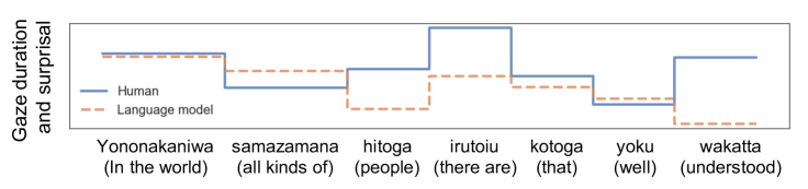
More concretely, over three dozens of LMs were trained for each language, with variants in their architecture, training data size, and the number of parameter updates. Then, the surprisals computed by each LM were compared to human eye movement data (Figure 1). The analysis of the relationship between PPL and the psychometric predictive power revealed substantively different trends between the Japanese and English LMs. In Japanese, a lower PPL of a LM does not indicate better performance for modeling reading behavior. By contrast, in English, there was a clear relationship between the two metrics as reported in the prior studies.

This opens a remaining and important question: why are English and Japanese different in this aspect? We discuss the differing results between English and Japanese from the perspective of the uniform information density hypothesis Genzel and Charniak (2002); Levy (2005); Jaeger and Levy (2007). We find that the processing difficulty (i.e., gaze duration) of segments is less uniformly distributed within a Japanese sentence. Given this, the discrepancy of the results between English and Japanese might stem from a mismatch between the information uniformity of the target language and the LM’s training objective. We demonstrate that tuning Japanese LMs to this training objective collapses the human-like nonuniformity of the processing difficulty observed in Japanese subjects. Our code is made publicly available.¹¹1https://github.com/kuribayashi4/surprisal_reading_time_en_ja

2 Related work

2.1 Human sentence processing and LMs

What factor determines the incremental difficulty of human language processing? At present, surprisal theory Hale (2001); Levy (2008) has been widely adopted in the field of computational psycholinguistics. This theory suggests that the processing difficulty of a segment is determined by how predictable the segment is in its preceding context ( $-\log{p(\mathrm{segment}|\mathrm{preceding\ context})}$ ).

Existing studies have compared various computational models by checking the effectiveness of their surprisals in modeling human reading behavior Hale (2001); Roark et al. (2009); Frank and Bod (2011); Fossum and Levy (2012); Hale et al. (2018); Goodkind and Bicknell (2018); Merkx and Frank (2020); Wilcox et al. (2020). Data such as eye movement Kennedy et al. (2003) and brain activity Frank et al. (2015); Brennan et al. (2016) are used as measures of human reading behavior. For example, using eye movement data, Frank and Bod (2011) compared the surprisals from phrase-structure grammars (PSGs) with those from a non-hierarchical, sequential model, tentatively concluding that human sentence processing was insensitive to hierarchical structures since non-hierarchical models displayed better psychological predictive power than PSGs. Recently, researchers reported that surprisals from LMs with low PPL correlate well with human reading behaviors Fossum and Levy (2012); Goodkind and Bicknell (2018); Aurnhammer and Frank (2019); Wilcox et al. (2020).

The work most closely related to this study is Wilcox et al. (2020). They examined the relationship between PPL, psychometric predictive power, and syntactic knowledge in LMs using a variety of models, including modern neural LMs Radrof et al. (2018). They found a tight relationship between PPL and psychometric predictive power in the English corpora. This study investigates whether this relationship can be generalized across languages.

2.2 Reading behavior in Japanese

In comparison to English speakers, Japanese speakers display different patterns in sentence processing. For example, an anti-locality effect (the more modifiers a word has in its preceding context, the easier the word is to process) has typically been observed in head-final languages, including Japanese Konieczny (2000). Such differences between the languages are assumed to be more or less due to their different sentence structures. Recently, eye movement data for naturally occurring Japanese texts have recently become available Asahara et al. (2016) and was extensively annotated with various linguistic properties Asahara and Kato (2017); Asahara (2017, 2018).

3 Methods

This section describes the settings of LMs, eye movement data, and evaluation metrics.

3.1 Language models

A variety of sentence-level, left-to-right sequential LMs was used.

Training data of English LMs:

We used the WikiText-103 dataset to train the English LMs. Based on the reports that subword-level English LMs exhibits superior psychometric predictive power Wilcox et al. (2020), input texts were divided into subwords by a byte-pair encoding (BPE) Sennrich et al. (2016).²²2Implemented in SentencePiece Kudo and Richardson (2018). We set character coverage to 0.9995，and vocabulary size to 32,000 in English. In Japanese, the vocabulary size is 100,000, reflecting its rich morphemes. The training data consist of approximately 4M sentences (114M subwords units).

Training data of Japanese LMs:

We used news articles and the Japanese part of Wikipedia to train the Japanese LMs. Input texts were first segmented into morphemes by MeCab Kudo (2006) with unidic dictionary, and then further divided into subwords by BPE.²²footnotemark: 2 The training data consist of approximately 5M sentences (146M subwords units).

Architectures:

The following four variants of LMs were used: Transformer-large (Trans-lg) Vaswani et al. (2017), Transformer-small (Trans-sm), LSTM (LSTM) Hochreiter and Schmidhuber (1997), and N-gram LMs (N-gram).³³3The neural LMs were trained with the fairseq toolkit Ott et al. (2019). N-gram LMs were trained using KenLM https://github.com/kpu/kenlm. The parameter size was almost the same for Trans-sm and LSTM. With respect to the N-gram models, 3-gram, 4-gram, and 5-gram LMs were used. Appendix A shows the hyperparameters of the neural LMs.

Training data size:

For each neural LM architecture (Trans-lg, Trans-sm, and LSTM), three variants were trained using different training data sizes: lg (full training data), md (1/10 training data), and sm (1/100 training data). The N-gram LMs were trained on lg datasets.

Number of updates:

The parameters of each neural LM were saved at four different points during training: 100, 1K, 10K, and 100K parameter updates.

To summarize, 39 LM training settings were attained for each language (3 architectures $\times$ 3 data size $\times$ 4 parameter updates $=$ 36 neural LMs, plus 3 N-gram LMs). In addition, our experiments use three LMs trained using different random seeds for each neural LM training configure; hence, 111 LMs (36 neural LMs $\times$ 3 seeds, plus 3 N-gram LMs) were tested for each language.

Corpus	#articles	#sents.	#segments	#data points (used)	#subjects per article	Avg. GD per segment	Avg. #subwords per segment
Dundee Corpus	20	2,478	51,501	214,955	10	227.1	1.3
BCCWJ-EyeTrack	20	218	1,643	6,009	12	361.6	3.4

Table 1: Statistics of the corpora used for evaluating the psychometric predictive power of LMs. “#articles” and “#sents.” are the number of articles and sentences in each corpus. “#segments” denotes the number of segments annotated with human reading time in each corpus. “#data points” is the number of reading time annotations used in our experiments. Each segment has the reading time annotations from multiple subjects (#subjects per article). “Avg. GD per segment” is the averaged gaze duration per segment. “Avg. #subwords per segment” denotes the averaged number of subwords consisting of each segment.

3.2 Eye movement data

English:

The Dundee Corpus Kennedy et al. (2003), which contains gaze duration annotation for each word, was used. Following Smith and Levy (2013), the first-pass gaze duration was analyzed. Then, following Goodkind and Bicknell (2018), the data points that met any of the following criteria were excluded:

•

data points with zero gaze duration or that beyond three standard deviations
•

segments with punctuation or numeric characters
•

segments whose next segment has punctuation or numeric characters
•

first or last segment in a line

In total, the analysis included 214,955 data points in the corpus.

Japanese:

The BCCWJ-EyeTrack Asahara et al. (2016), which contains gaze duration annotation for each phrasal unit, was used. Note that the phrasal unit (i.e., bunsetsu) consists of at least one content morpheme and its postpositional function morphemes. Henceforth, an English word and a Japanese phrasal unit are referred to as a “segment.” The same exclusion criteria as the Dundee Corpus was applied to the BCCWJ-EyeTrack data.⁴⁴4Strictly speaking, the exclusion criteria was slightly different between Japanese and English data. In the Japanese data, we included the segments whose next segment had punctuation or a numeric character, as there is no spillover effect in Japanese (see Section 3.3) In total, the analysis included 6,009 data points in the corpus. Note that the BCCWJ-EyeTrack data was deliberately designed to address language-specific issues in Japanese such as the lack of segmentation spaces in Japanese texts Asahara et al. (2016).

Statistics:

Table 1 shows the statistics of the Dundee Corpus and BCCWJ-EyeTrack data. The BCCWJ-EyeTrack has more than 10 times a smaller number of data points than the Dundee Corpus. Notably, the segment annotated with eye movement information differs between English and Japanese. On average, a Japanese segment consists of 3.4 subwords, while an English segment consists of 1.3 subwords. Smith and Levy (2013) theoretically proved that the more fragments a word is divided into when computing its surprisal, the better the calculated surprisal approximates the human cognitive effort if the human language processing is highly incremental. Thus, we tentatively consider that this difference did not make a negative impact on the results using the Japanese data.

3.3 Evaluation metrics

Perplexity (PPL):

PPL, the inverse geometric mean of next-word probabilities $p(w_{i}|w_{<i})$ in a text that consists of $N$ signals ( $w_{1},w_{2},\cdots,w_{N}$ ), is a typical evaluation metric for unidirectional LMs (Eq. 1):

PPL

\displaystyle=\prod_{i=0}^{N}p(w_{i}|w_{<i})^{-\frac{1}{N}}\>\>.

(1)

Low PPL indicates that the model can accurately predict the upcoming signal based on its preceding context. The training objective of LMs works to minimize the PPL computed by the model. In the experiments, the PPL of a LM is evaluated with the texts in the eye movement data, which do not overlap with the training data. A model with low PPL is also called a linguistically accurate model Frank and Bod (2011).

Psychometric predictive power:

The surprisal measure, a negative logarithmic probability of a segment in context ( $-\log{p({\rm segment}|{\rm preceding\ context})}$ ), is a widely used information-theoretic complexity metric. Intuitively, a model is considered to have high psychometric predictive power (i.e., psychological accuracy) if the surprisals of segments computed by the model have trends similar to the human subject’s cognitive load (e.g., measured by gaze duration). Following the existing studies Goodkind and Bicknell (2018); Merkx and Frank (2020); Wilcox et al. (2020), the psychometric predictive power of a model was measured by comparing surprisal from the model and gaze duration from human subjects.

While LMs process a text subword-by-subword, gaze duration is annotated in a larger segment. Following the study using subwords Wilcox et al. (2020), the surprisal of each segment was calculated using the joint probability of its constituent subwords. Formally, given a text consisting of $N$ subwords $w_{1:N}=(w_{1},w_{2},\cdots,w_{N})$ , surprisal $I(\cdot)$ of a segment $s_{k}=(w_{l},w_{l+1},\cdots,w_{m})$ , where $1\leq l\leq m\leq N$ , was calculated as follows:

\displaystyle\begin{split}I(s_{k})&=-\log p(w_{l},\cdots,w_{m}|w_{<l})\\ &=-\sum_{k=l}^{m}\log p(w_{k}|w_{1},\cdots,w_{k-1})\>\>.\end{split}

(2)

The effect of surprisals for modeling human reading behavior was calculated using a linear mixed-effects regression Bates et al. (2015). Specifically, the gaze duration (GD) was modeled using the following formula:

\displaystyle\begin{split}\texttt{GD}&\sim\texttt{surprisal}+\texttt{surprisal\_prev\_1}\\ &+\texttt{surprisal\_prev\_2}+\texttt{freq}*\texttt{length}\\ &+\texttt{freq\_prev\_1}*\texttt{length\_prev\_1}\\ &+\texttt{screenN}+\texttt{lineN}+\texttt{segmentN}\\ &+\texttt{(1|article)}+\texttt{(1|subj)}\>\>.\end{split}

(3)

The regression model includes baseline factors (e.g., frequency of a segment) that are of no interest in the comparison of LMs. A collection of factors used in the existing studies Asahara et al. (2016); Wilcox et al. (2020) were initially examined and the factors that were not significant ( $p>0.05$ ) for gaze duration modeling both in the Dundee Corpus and BCCWJ-EyeTrack were excluded. The frequency of a segment (freq) was calculated using the entire training data for LMs. Appendix B shows the details of each factor in Eq. 3.

In English experiments, surprisals of preceding words (surprisal_prev_1 and surprisal_prev_2) were included in order to handle the spillover effect (the processing cost of a certain segment is affected by its preceding segments) Rayner and Well (1996); Smith and Levy (2013). In Japanese experiments, the surprisals of preceding words were not included because our preliminary experiment showed that these factors were not significantly effective for modeling gaze duration in the BCCWJ-EyeTrack.⁵⁵5The reason is probably that a Japanese phrasal unit (i.e., bunsetsu) could be a larger unit than an English word. All the regression models used in our experiments were converged.

To isolate the effect of surprisal for gaze duration modeling, a baseline regression model was trained without surprisal information (excluding the surprisal, surprisal_prev_1, and surprisal_prev_2 terms from Eq. 3). Following Wilcox et al. (2020), the mean by-segment difference of log-likelihood between the model using surprisal values (Eq. 3) and the baseline model was calculated. Henceforth, this metric is called $\Delta$ LogLik. When surprisal from a LM is not effective for gaze duration modeling, the $\Delta$ LogLik score becomes zero. A high $\Delta$ LogLik means that the surprisal values obtained by the LM are effective for modeling gaze duration (i.e., the LM has a high psychometric predictive power).

4 Experiments

The relationship between PPL and psychometric predictive power is investigated. Furthermore, the relationship is analyzed with respect to the training configures of LMs (e.g., the number of parameter updates). Then, we discuss the results from the perspective of the uniformity of information density.

4.1 Psychometric predictive power and PPL

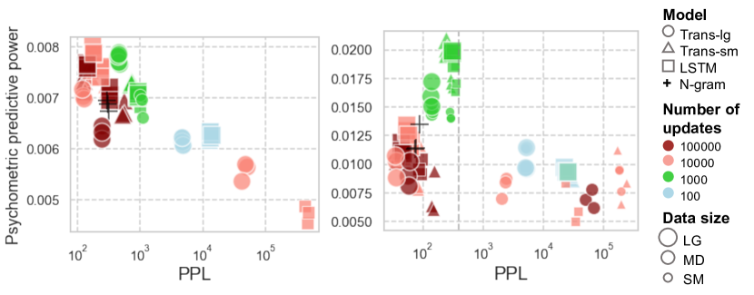
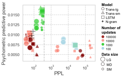
Figure 2 shows the relationship between PPL and psychometric predictive power (i.e., $\Delta$ LogLik) of LMs in each of the languages. Each point corresponds to each LM, and a score on the Y-axis indicates the psychometric predictive power of a LM (higher is better). The X-axis is PPL on a log scale (lower is better).

Dundee Corpus:

First, the results of the data from the Dundee Corpus show a clear relationship between PPL and psychometric predictive power; namely, lower PPL corresponds to more psychometric predictive power, as reported by prior studies Goodkind and Bicknell (2018); Wilcox et al. (2020). Spearman’s rank correlation coefficient between the two metrics was $-0.87$ .

BCCWJ-EyeTrack:

By contrast, in BCCWJ-EyeTrack, there was no clear, consistent trend between the PPL and psychometric predictive power. While LMs with PPL over 400 show the correlation between PPL and psychometric predictive power ( $-0.68$ with Spearman’s $\rho$ ), there is a positive correlation ( $0.53$ with Spearman’s $\rho$ ) for LMs with PPL below 400. The positive correlation means that the more accurately the LMs can predict the upcoming word, the worse the psychometric predictive power of the LMs is. These results demonstrate the non-universality of the recent report across languages; lower perplexity is not always human-like. The lstm LM trained using the md dataset with 1K updates achieved the best psychometric predictive power. Notably, surprisal was effective for gaze duration modeling in all the Japanese LMs. $\Delta$ logLik scores were significantly higher than zero with the chi-square test ( $p<$ 0.05).

4.2 Model architectures, data sizes, number of parameter updates

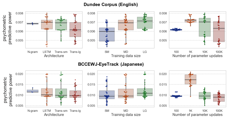
Which factor (e.g., model architecture, training data size, and the number of parameter updates) characterizes the psychometric predictive power of LMs? Is the collection of effective factors consistent between the two languages? This study takes a more in-depth look at the separate effects of (i) model architecture, (ii) training data size, and (iii) the number of parameter updates for the psychometric predictive power.

Figure 3 summarizes the effect of each factor, where the Y-axis denotes the psychometric predictive power. The most noticeable trend is that Japanese LMs with a relatively fewer number of parameter updates (1K) have better psychometric predictive power than the other Japanese LMs (bottom right part of Figure 3), while this trend does not exist in the English LMs (top right part). This implies that the training objective of the LMs, maximizing $\frac{1}{N}\sum_{i=1}^{N}\log P(w_{i}|w_{<i})$ , had a negative impact on the psychometric predictive power of LMs, at least in Japanese. We discuss this point in Section 4.3.

To quantitatively test the differences in Figure 3, a linear regression model was trained to estimate psychometric predictive power with the factors of the model architecture, the training data size, and the parameter update number in each language. The training data size and the parameter update number are represented as logarithmically transformed numerical factors. The following trends were found: (i) ; (ii) the training data size positively affects the performance in English alone; and (iii) the number of parameter updates positively affects the performance only in English. There was no factor that boosted the psychometric predictive power of LMs in both English and Japanese languages.

4.3 Discussion: uniform information density

The key question is: why do Japanese and English show different trends between PPL and psychometric predictive power? One possible interpretation connecting our results to the uniform information density is discussed in this section.

In computational psycholinguistics, it is commonly assumed that language is designed to enable efficient communication. This principle has been typically investigated under the uniform information density (UID) hypothesis Genzel and Charniak (2002); Levy (2005); Jaeger and Levy (2007). This hypothesis suggests that speakers seek to keep the amount of information constant across the signals (e.g., segments).

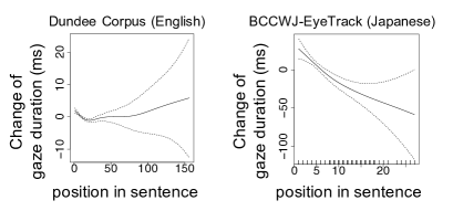
Assuming this hypothesis holds for all languages, the reasonable expectation would be for human subjects to show a near-uniform gaze duration across segments regardless of their native language. However, this study found that the coefficient of variation⁶⁶6Coefficient of variation is $\frac{\sigma}{\mu}$ , where $\sigma$ and $\mu$ are the standard deviation and the mean of the first-pass gaze durations in the eye movement data. in gaze duration over the whole corpus was around 1.7 times higher in Japanese compared to English (0.75 vs. 0.44). Specifically, in Japanese, the gaze duration tended to speed up towards the end of sentences, whereas the duration was near-uniform in English (Figure 4).⁷⁷7At least in our experimental setup, token position within the sentence was not significantly effective for gaze duration modeling in English sentences, whereas it was significant in Japanese sentences. We checked the coefficient of the factor of position in sentence segmentN using the linear regression model of GD $\sim$ sengmentN. These observations imply that the Japanese language might have a less uniform information density than English. This phenomenon was also investigated through the lens of word order, where SOV languages such as Japanese are reported to show less uniformity of information density Maurits et al. (2010).

Based on this observation, the discrepancy between English and Japanese low-PPL LMs’ psycholinguistic predictive power could stem from a mismatch between the LM’s training objective and the information uniformity of the target language. The objective function, $\frac{1}{N}\sum_{i=1}^{N}\log P(w_{i}|w_{<i})$ , defines that the “ideal” is to maximize all next word probabilities to 1.0 (a uniform goal).⁸⁸8PPL, $\prod_{i=1}^{N}P(w_{i}|w_{<i})^{-\frac{1}{N}}$ , is minimized when the LM objective are maximized. That is, LMs are, in theory, trained to approach a model satisfying the UID assumption Bloem (2016), where all surprisals from the LM are equally, sufficiently small across the segments. Therefore, the objective function might lead to a worse approximation of human-like surprisal in languages that are further from the UID assumption, such as Japanese, while it might be more compatible with English, which has a more uniform processing difficulty across segments. This explanation would be consistent with the observation that more tuning to the LM training objective (i.e., a lower PPL) had a negative impact on the psycholinguistic performance of the Japanese LMs (Section 4.2). Note the tendency of LMs to assign unreasonably high probabilities to segments has also attracted attention from the viewpoint of memorization capability of LMs Carlini et al. (2020). In addition, the connection of the UID hypothesis to the modern NLP techniques has been recently explored Meister et al. (2020); Wei et al. (2021). We further investigate our hypothesis in Section 5.

5 Probing nonuniform information density of Japanese LMs

This study hypothesized that tuning to the LM objective (i.e., uniform goal) obscures the nonuniform trend observed in the reading behavior of Japanese subjects. We investigated whether the nonuniformity of the processing difficulty observed in human reading time is mirrored by LM surprisals.

Settings:

In a preliminary experiment, we observed that the syntactic category (similar to part-of-speech) was the most dominant linguistic factor for explaining the difference in human gaze duration in Japanese sentences (see Appendix D). Based on this observation, we analyze the nonuniformity of surprisals in Japanese LMs with respect to the syntactic categories.

The segments in BCCWJ-EyeTrack were classified into one of the following syntactic categories: (a) nominal (nouns), (b) verbal (verbs), (c) modifier (adjectives and adverbs), and (d) other entries, as follows:

As Asahara and Kato (2017) reported, verbal and modifier segments have a shorter gaze duration than the other segments in Japanese sentences. An analysis was conducted on how strongly the Japanese LM’s surprisals on segments are influenced by their syntactic category. This influence can be evaluated by examining how effectively syntactic category factors can model LM surprisals.

In this experiment, surprisal was regarded as “simulated gaze duration” from an “LM subject,” and the importance of syntactic category information for modeling the simulated gaze duration (simulated_GD) was evaluated. To inspect the effect of the syntactic category information for modeling the simulated gaze duration, the following regression model⁹⁹9sentN and tokenN denote the sentence position and the segment position in a sentence (see Appendix B). Note that the tokenN and syntactic category exhibit low correlation (0.02 with Pearson’s $r$ ). was used, including a factor defining which syntactic category the segment falls into (syn_category):

\displaystyle\begin{split}\texttt{simulated\_GD}&\sim\texttt{syn\_category}+\texttt{sentN}\\ &+\texttt{tokenN}+\texttt{freq}*\texttt{length}\>\>.\end{split}

(4)

From this regression model, a log-likelihood score for the simulated gaze duration was obtained. To evaluate the separate effect of syn_category, $\Delta$ LogLik between Eq. 4 and a baseline model was calculated. The baseline model was $\texttt{simulated\_GD}\sim\texttt{sentN}+\texttt{tokenN}+\texttt{freq}*\texttt{length}$ . The $\Delta$ LogLik is denoted as “Effect of syntactic category.” A lower score means that the LM lacked the property of varying processing difficulty with respect to the syntactic category.

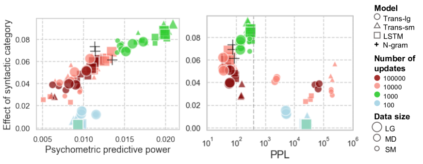
Results:

The results are shown in Figure 5. First, the higher psychometric predictive power the LMs exhibit, the greater the effect of syntactic category on surprisals (left part in Figure 5). This means that, depending on the syntactic category of the segment they processed, LMs with high psychometric predictive power computed surprisals with a more nonuniform trend. The right part of Figure 5 shows that, as PPL decreases below a certain value ( $\mathrm{PPL}\sim 400$ ), the Japanese LMs compute surprisals that obscure the nonuniform trends with respect to the syntactic category of segments.¹⁰¹⁰10The correlation between PPL and the effect of syntactic category in the LMs with PPL less than 400 was 0.45 and 0.34 with Pearson’s $r$ and Spearman’s $\rho$ , respectively. This trend supports our hypothesis that tuning to LM objectives obscures the human-like nonuniformity of the processing difficulty. Even though LMs that are not fully tuned to the LM objective ( $\mathrm{PPL}\sim 400$ ) acquire human-like trends with respect to syntactic category, these biases tend to be lost by further lowering their PPL.

Notably, we also observed that not all the types of linguistic nonuniformity were obscured in surprisals computed by the LMs with low PPL. For example, Appendix E shows that LMs with lower PPL compute surprisals that better correlates with a particular syntactic factor although that factor is a less dominant trend in human reading behavior than the syntactic category (Appendix D).

6 Limitations and future works

To test the universality of the recent findings in computational psycholinguistics across languages, the initial focus is on English and Japanese as a pair of languages with different linguistic properties. Although the discrepancy of the results in the two languages is discussed from the viewpoint of the UID hypothesis, the two languages are also different in various ways, such as writing systems, agglutinative property, case marking, sentence structure, and pro-drop nature. To identify the difference that relates to the human-like behaviors of LMs, experiments that include additional languages should be conducted in the future.

In addition, the corpus size of the BCCWJ-EyeTrack data is smaller than the Dundee Corpus. While the reading time data in the BCCWJ-EyeTrack was collected from various human subjects, the number of the independent segments was limited (1,643 segments, 218 sentences). Thus, whether the trends reported in this study generalize to more diverse Japanese texts should be explored in future work. It is hoped that this study motivates the creation of a large-scale corpus of human reading behaviors in diverse languages.

7 Conclusion

This study has investigated whether the recent reports on the psychometric predictive power of LMs can be generalized across languages. Our initial investigation has re-examined the recent report—the lower PPL a LM has, the more human-like the LM is—using Japanese eye movement data. Our experiments have demonstrated a surprising lack of universality of this report; lower perplexity is not always human-like. This discrepancy of the results between the languages reinforces the need for the cross-lingual evaluation of the psychometric predictive power of LMs. The discussion considers potential factors that make the observation different across languages from the viewpoint of the uniform information density hypothesis. We believe that this is an important first step for seeking a language-agnostic model of human sentence processing. Hopefully, this study encourages researchers to further investigate the universality of human language processing across languages.

Acknowledgements

We would like to thank the members at the Tohoku NLP Lab for their valuable advice, particularly Ana Brassard for proofreading. This work was supported by Grant-in-Aid for JSPS Fellows Grant Number JP20J22697, JSPS KAKENHI Grant Number 19H04990, and JST CREST Grant Number JPMJCR20D2. This work was also supported by the National Institute for Japanese Language and Linguistics (NINJAL) Collaborative Research Project “Computational Psycholinguistics of Language Processing with Large Corpora.”

Ethical considerations

Language models with low perplexity are typically trained with a high computational cost. Our work demonstrates that further up-scaling the models might not be a reasonable direction of searching for human-like language models. This could potentially contribute to reducing energy and carbon costs, which are needed to train large-scale language models.

References

Asahara (2017) Masayuki Asahara. 2017. Between Reading Time and Information Structure. In Proceedings of PACLIC, pages 15–24.
Asahara (2018) Masayuki Asahara. 2018. Between Reading Time and Clause Boundaries in Japanese - Wrap-up Effect in a Head-final Language. In Proceedings of PACLIC, pages 19–27.
Asahara and Kato (2017) Masayuki Asahara and Sachi Kato. 2017. Between Reading Time and Syntactic / Semantic Categories. In Proceedings of IJCNLP, pages 404–412.
Asahara et al. (2016) Masayuki Asahara, Hajime Ono, and Edson T Miyamoto. 2016. Reading-Time Annotations for “Balanced Corpus of Contemporary Written Japanese”. In Proceedings of COLING, pages 684–694.
Aurnhammer and Frank (2019) C Aurnhammer and S L Frank. 2019. Comparing Gated and Simple Recurrent Neural Network Architectures as Models of Human Sentence Processing. In Proceedings of CogSci, pages 112–118.
Bates et al. (2015) Douglas Bates, Martin Mächler, Ben Bolker, and Steve Walker. 2015. Fitting linear mixed-effects models using lme4. Journal of Statistical Software, Articles, 67(1):1–48.
Bender (2011) Emily M Bender. 2011. On Achieving and Evaluating Language-Independence in NLP. Linguistic Issues in Language Technology, 6(3):1–26.
Bloem (2016) Jelke Bloem. 2016. Testing the processing hypothesis of word order variation using a probabilistic language model. In Proceedings of the Workshop on Computational Linguistics for Linguistic Complexity (CL4LC), pages 174–185, Osaka, Japan. The COLING 2016 Organizing Committee.
Brennan et al. (2016) Jonathan R Brennan, Edward P Stabler, Sarah E Van Wagenen, Wen-Ming Luh, and John T Hale. 2016. Abstract linguistic structure correlates with temporal activity during naturalistic comprehension. Brain and language, 157:81–94.
Brown et al. (2020) Tom B Brown, Benjamin Mann, Nick Ryder, Melanie Subbiah, Jared Kaplan, Prafulla Dhariwal, Arvind Neelakantan, Pranav Shyam, Girish Sastry, Amanda Askell, Sandhini Agarwal, Ariel Herbert-Voss, Gretchen Krueger, Tom Henighan, Rewon Child, Aditya Ramesh, Daniel M Ziegler, Jeffrey Wu, Clemens Winter, Christopher Hesse, Mark Chen, Eric Sigler, Mateusz Litwin, Scott Gray, Benjamin Chess, Jack Clark, Christopher Berner, Sam McCandlish, Alec Radford, Ilya Sutskever, and Dario Amodei. 2020. Language Models are Few-Shot Learners. In Proceedings of NeurIPS.
Carlini et al. (2020) Nicholas Carlini, Florian Tramèr, Eric Wallace, Matthew Jagielski, Ariel Herbert-Voss, Katherine Lee, Adam Roberts, Tom B. Brown, Dawn Song, Úlfar Erlingsson, Alina Oprea, and Colin Raffel. 2020. Extracting training data from large language models. CoRR, abs/2012.07805.
Demberg and Keller (2008) Vera Demberg and Frank Keller. 2008. Data from eye-tracking corpora as evidence for theories of syntactic processing complexity. Journal of Cognition, 109(2):193–210.
Fossum and Levy (2012) Victoria Fossum and Roger Levy. 2012. Sequential vs. Hierarchical Syntactic Models of Human Incremental Sentence Processing. In Proceedings of CMCL, pages 61–69, Montréal, Canada.
Frank and Bod (2011) Stefan L Frank and Rens Bod. 2011. Insensitivity of the Human Sentence-Processing System to Hierarchical Structure. Psychological science, 22(6):829–834.
Frank et al. (2015) Stefan L. Frank, Leun J. Otten, Giulia Galli, and Gabriella Vigliocco. 2015. The erp response to the amount of information conveyed by words in sentences. Brain and Language, 140:1–11.
Genzel and Charniak (2002) Dmitriy Genzel and Eugene Charniak. 2002. Entropy rate constancy in text. In Proceedings of the 40th Annual Meeting of the Association for Computational Linguistics, pages 199–206, Philadelphia, Pennsylvania, USA. Association for Computational Linguistics.
Goodkind and Bicknell (2018) Adam Goodkind and Klinton Bicknell. 2018. Predictive power of word surprisal for reading times is a linear function of language model quality. In Proceedings of CMCL2018, pages 10–18.
Hale (2001) John Hale. 2001. A Probabilistic Earley Parser as a Psycholinguistic Model. In Proceedings of NAACL, pages 159–166.
Hale et al. (2018) John Hale, Chris Dyer, Adhiguna Kuncoro, and Jonathan R. Brennan. 2018. Finding Syntax in Human Encephalography with Beam Search. In Proceedings of ACL, pages 2727–2736.
Hochreiter and Schmidhuber (1997) Sepp Hochreiter and Jürgen Schmidhuber. 1997. Long Short-Term Memory. Journal of Neural Computation, 9(8):1735–1780.
Jaeger and Levy (2007) T Jaeger and Roger Levy. 2007. Speakers optimize information density through syntactic reduction. In Advances in Neural Information Processing Systems, volume 19, pages 849–856. MIT Press.
Kaplan et al. (2020) Jared Kaplan, Sam McCandlish, Tom Henighan, Tom B Brown, Benjamin Chess, Rewon Child, Scott Gray, Alec Radford, Jeffrey Wu, and Dario Amodei. 2020. Scaling Laws for Neural Language Models. arXiv preprint arXiv:2001.08361.
Kennedy et al. (2003) Alan Kennedy, Robin Hill, and Joël Pynte. 2003. The dundee corpus. In Proceedings of the 12th European conference on eye movement.
Konieczny (2000) Lars Konieczny. 2000. Locality and Parsing Complexity. Journal of Psycholinguistic Research, 29(6):627–645.
Kudo (2006) Taku Kudo. 2006. MeCab: Yet Another Part-of-speech and Morphological Analyzer. http://mecab. sourceforge. jp.
Kudo and Richardson (2018) Taku Kudo and John Richardson. 2018. SentencePiece: A simple and language independent subword tokenizer and detokenizer for Neural Text Processing. In Proceedings of EMNLP, pages 66–71.
Levy (2005) Roger Levy. 2005. Probabilistic models of word order and syntactic discontinuity. stanford university.
Levy (2008) Roger Levy. 2008. Expectation-based syntactic comprehension. Journal of Cognition, 106(3):1126–1177.
Maurits et al. (2010) Luke Maurits, Dan Navarro, and Amy Perfors. 2010. Why are some word orders more common than others? a uniform information density account. In Advances in Neural Information Processing Systems, volume 23. Curran Associates, Inc.
Meister et al. (2020) Clara Meister, Ryan Cotterell, and Tim Vieira. 2020. If beam search is the answer, what was the question? In Proceedings of the 2020 Conference on Empirical Methods in Natural Language Processing (EMNLP), pages 2173–2185, Online. Association for Computational Linguistics.
Merkx and Frank (2020) Danny Merkx and Stefan L. Frank. 2020. Human Sentence Processing: Recurrence or Attention? In Procceding of CMCL 2021.
Ott et al. (2019) Myle Ott, Sergey Edunov, Alexei Baevski, Angela Fan, Sam Gross, Nathan Ng, David Grangier, and Michael Auli. 2019. fairseq: A fast, extensible toolkit for sequence modeling. In Proceedings of the 2019 Conference of the North American Chapter of the Association for Computational Linguistics (Demonstrations), pages 48–53, Minneapolis, Minnesota. Association for Computational Linguistics.
Radrof et al. (2018) Alec Radrof, Jeffrey Wu, Rewon Child, David Luan, Dario Amodei, and Ilya Sutskever. 2018. Language Models are Unsupervised Multitask Learners. Technical report, OpenAI.
Rayner and Well (1996) Keith Rayner and Arnold D Well. 1996. Effects of contextual constraint on eye movements in reading: A further examination. Psychonomic Bulletin & Review, 3(4):504–509.
Roark et al. (2009) Brian Roark, Asaf Bachrach, Carlos Cardenas, and Christophe Pallier. 2009. Deriving lexical and syntactic expectation-based measures for psycholinguistic modeling via incremental top-down parsing. In Proceedings of EMNLP, pages 324–333, Singapore.
Sennrich et al. (2016) Rico Sennrich, Barry Haddow, and Alexandra Birch. 2016. Neural Machine Translation of Rare Words with Subword Units. In Proceedings of ACL, pages 1715–1725.
Smith and Levy (2013) Nathaniel J. Smith and Roger Levy. 2013. The effect of word predictability on reading time is logarithmic. Journal of Cognition, 128(3):302–319.
Vaswani et al. (2017) Ashish Vaswani, Noam Shazeer, Niki Parmar, Jakob Uszkoreit, Llion Jones, Aidan N. Gomez, Łukasz Kaiser, and Illia Polosukhin. 2017. Attention Is All You Need. In Proceedings of NIPS, pages 5998–6008.
Wei et al. (2021) Jason Wei, Clara Meister, and Ryan Cotterell. 2021. A cognitive regularizer for language modeling. arXiv preprint arXiv:2105.07144.
Wilcox et al. (2020) Ethan Gotlieb Wilcox, Jon Gauthier, Jennifer Hu, Peng Qian, and Roger Levy. 2020. On the Predictive Power of Neural Language Models for Human Real-Time Comprehension Behavior. In Proceedings of CogSci, pages 1707–1713.

Appendix A Hyperparameters of LMs

Table 2 shows the hyperparameters of Trans-sm, Trans-lg, and LSTM, respectively. Note that the number of parameter updates varies as described in Section 3.

Fairseq model	architecture	transformer_lm_gpt2_small
	adaptive softmax cut off	50,000, 140,000
	share-decoder-input-output-embed	True
	embed_dim	1,024
	ffn_embed_dim	4,096
	layers	24
	heads	16
	dropout	0.1
	attention_dropout	0.1
Optimizer	algorithm	AdamW
	learning rates	5e-4
	betas	(0.9, 0.98)
	weight decay	0.01
	clip norm	0.0
Learning rate scheduler	type	inverse_sqrt
	warmup updates	4,000
	warmup init lrarning rate	1e-7
Training	batch size	61,440 tokens
Training	sample-break-mode	none

(a) Trans-lg.

Fairseq model	architecture	transformer_lm_gpt
	adaptive softmax cut off	50,000, 140,000
	share-decoder-input-output-embed	True
	embed_dim	384
	ffn_embed_dim	2,048
	layers	8
	heads	6
	dropout	0.1
	attention_dropout	0.1
Optimizer	algorithm	AdamW
	learning rates	5e-4
	betas	(0.9, 0.98)
	weight decay	0.01
	clip norm	0.0
Learning rate scheduler	type	inverse_sqrt
	warmup updates	4,000
	warmup init lrarning rate	1e-7
Training	batch size	61,440 tokens
Training	sample-break-mode	none

(b) Trans-sm.

Fairseq model	architecture	lstm_lm
	adaptive softmax cut off	50,000, 140,000
	share-decoder-input-output-embed	True
	embed_dim	400
	hiden_size	1,024
	layers	2
	dropout	0.1
Optimizer	algorithm	AdamW
	learning rates	1e-3
	betas	(0.9, 0.98)
	weight decay	0.01
	clip norm	0.0
Learning rate scheduler	type	inverse_sqrt
	warmup updates	4,000
	warmup init lrarning rate	1e-7
Training	batch size	20,480 tokens
Training	sample-break-mode	none

Table 2: Hyperparameters for the LMs.

Appendix B Factors used in regression models

Descriptions for the factors used in our experiments are shown in Table 3. The frequency of a segment (freq) was estimated using the full training data for the LMs.

Factor name	Type	Description
surprisal	num	surprisal caluzulted by LMs
GD	num	reading time (first pass time)
article	factor	article ID
screenN	int	screen display order
lineN	int	the serial number of line the segment is displayed
segmentN	int	the serial number of segment in a screen
sentN	int	the serial number of sentence the segment belongs to
tokenN	int	the position of segment in sentence
length	int	number of characters
freq	num	geometric mean of the frequencies of subword constituents in a segment
subj	factor	participant ID
syn_category	factor	syntactic category the segment falls into (nominal, verbal, modifier, or other)
sem_category	factor	semantic category the segment falls into (relation, subject, action, product, or nature)
n_dependents	int	number of dependents before the segment

Table 3: Factor names and their description.

syntactic category	number of segments	Avg. gaze duration
nominal	4,322	388.4
verbal	1,090	291.0
modifier	588	297.1
other	9	239.3

Table 4: The statistics of the syntactic category labels in BCCWJ-EyeTrack.

Appendix C Results of modeling logarithmic gaze duration in BCCWJ-EyeTrack

Existing studies Asahara et al. (2016) performed experiments using the logarithmic gaze duration because the logarithmic gaze duration more matches the normal distribution than the raw gaze duration. Given this, we additionally conducted experiments in Section 4, changing the target variable from the raw gaze duration to its logarithmic gaze duration. The result with this setting is shown in Figure 6. There was no substantial difference with the results shown in Section 4.

Appendix D Preliminary experiments in Section 5

Which linguistic factor is helpful for explaining the difference in gaze duration? We conducted experiments using linguistic annotation in the BCCWJ-EyeTrack. Following the existing studies, we checked the separate effect of syntactic category, semantic category Asahara and Kato (2017), and a particular aspect of hierarchical syntactic structure (i.e., the anti-locality effect) Asahara et al. (2016). Specifically, we used the factors, syn_category, sem_category, and n_dependents, shown in Table 3. For each factor, we inspect the separate effect of each factor for modeling gaze duration. As Eq. 4, we first modeled the gaze duration using each factor (factor_X):

\displaystyle\begin{split}\texttt{GD}&\sim\texttt{factor\_X}+\texttt{sentN}\\ &+\texttt{segmentN}+\texttt{freq}*\texttt{length}\>\>.\end{split}

(5)

Then, we calculated the $\Delta$ LogLik between X and a baseline model. The baseline model was $\texttt{GD}\sim\texttt{sentN}+\texttt{segmentN}+\texttt{freq}*\texttt{length}$ .

The $\Delta$ LogLik for each collection of factors are shown in 5. We found that syntactic category is the most influential factor for modeling gaze duration, at least in this experiment.

linguistic property	$\Delta$ LogLik
syntactic category	58.37
semantic category	17.08
number of dependents	13.84

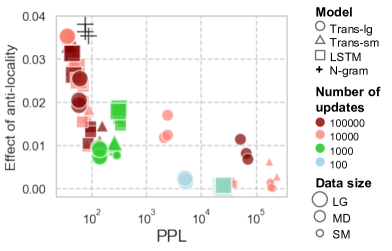
Table 5: The separate effect of each linguistic annotation for modeling gaze duration.

Appendix E Anti-locality effect in LMs

Similar to Section 5, we analyzed how strongly the surprisals from each Japanese LM are biased towards a particular linguistic property. In this section, we investigated the anti-locality effect in the surprisals from LMs. The anti-locality is that the more dependents a segment has in its preceding context, the cognitive effort of the head segment is reduced (i.e., modifiers alleviate the processing cost of their head).

Analogous to the Section 5, we regarded surprisal as “simulated gaze duration” from an “LM subject,” and evaluated the importance of the number of the dependents in its preceding context (n_dependents) for modeling the simulated gaze duration (simulated_GD). To inspect the effect of the n_dependents for modeling the simulated gaze duration, we used the following regression model:

\displaystyle\begin{split}\texttt{simulated\_GD}&\sim\texttt{n\_dependents}+\texttt{sentN}\\ &+\texttt{tokenN}+\texttt{freq}*\texttt{length}\>\>.\end{split}

(6)

From this regression model, we obtained a log-likelihood score for the simulated gaze duration. To evaluate the separate effect of n_dependents, we calculated the $\Delta$ LogLik between Eq. 6 and a baseline model. The baseline model was $\texttt{simulated\_GD}\sim\texttt{sentN}+\texttt{segmentN}+\texttt{freq}*\texttt{length}$ . The $\Delta$ LogLik is denoted as “Effect of the anti-locality.”

The results are shown in Figure 7. There is a clear trend that the LMs with lower PPL exhibit surprisals that are more consistent with the anti-locality effect (Spearman’s $\rho=-0.77$ between PPL and the strength of the anti-locality effect). This suggests that the surprisals from LMs with low PPL are biased towards the hierarchical structure of sentences rather than the syntactic category.