General Bayesian Loss Function Selection and the use of Improper Models

Abstract

Statisticians often face the choice between using probability models or a paradigm defined by minimising a loss function. Both approaches are useful and, if the loss can be re-cast into a proper probability model, there are many tools to decide which model or loss is more appropriate for the observed data, in the sense of explaining the data’s nature. However, when the loss leads to an improper model, there are no principled ways to guide this choice. We address this task by combining the Hyvärinen score, which naturally targets infinitesimal relative probabilities, and general Bayesian updating, which provides a unifying framework for inference on losses and models. Specifically we propose the $\mathcal{H}$-score, a general Bayesian selection criterion and prove that it consistently selects the (possibly improper) model closest to the data-generating truth in Fisher’s divergence. We also prove that an associated $\mathcal{H}$-posterior consistently learns optimal hyper-parameters featuring in loss functions, including a challenging tempering parameter in generalised Bayesian inference. As salient examples, we consider robust regression and non-parametric density estimation where popular loss functions define improper models for the data and hence cannot be dealt with using standard model selection tools. These examples illustrate advantages in robustness-efficiency trade-offs and enable Bayesian inference for kernel density estimation, opening a new avenue for Bayesian non-parametrics.

Keywords: Loss functions; Improper models; General Bayes; Hyvärinen score; Robust regression; Kernel density estimation.

1 Introduction

A common task in Statistics is selecting which amongst a set of models is most appropriate for an observed data set $y$. Tools to address this problem include a variety of penalised likelihood, shrinkage prior, and Bayesian model selection methods. Under suitable conditions, these approaches consistently select the model closest to the data-generating truth in Kullback-Leibler divergence (for example, see rossell:2021 and references therein for a recent discussion). However, many data analysis methods are not defined in terms of probability models but as minimising a given loss function, for example to gain robustness or flexibility. It is then no longer clear how to use the data to guide the choice of the most appropriate loss function, or its associated hyper-parameters. A key observation is that while the likelihood $f_{k}(y;\theta_{k})$ of a model $k$ with parameters $\theta_{k}$ always defines a loss function $\ell_{k}(y;\theta_{k})=-\log f_{k}(y;\theta_{k})$ (good1952rational), the converse is not true. The exponential of an arbitrary loss $f_{k}(y;\theta_{l})=\exp\{-\ell_{k}(y;\theta_{k})\}$ may not integrate to a finite constant and therefore, defines an improper model on $y$. For example, this occurs in robust regression with Tukey’s loss (Figure 2.1) and in kernel density estimation. There is also a growing literature following basu1998robust that applies the Tsallis score to define a robust loss function to fit any given probability model. Such robustification depends on a hyper-parameter that governs robustness-efficiency trade-offs and often leads to an improper model similar to Figure 2.1 (see Figure LABEL:Fig:TsallisTukeysLoss, and yonekura2021adaptation for a recent pre-print building on our improper model interpretation to address the hyper-parameter selection). In these scenarios traditional model selection tools are not applicable to choose the more appropriate loss. Neither are methods to evaluate predictive performance such as cross-validation, since they require specifying a loss or criterion to evaluate performance in the first place, and do not attain consistent model selection even in simple settings (shao1997asymptotic). Methods to tackle intractable but finite normalisation constants, such as approximate Bayesian computation (beaumont2002approximate, robert2016approximate), also do not apply since they require simulating from a proper model.

We propose methodology to evaluate how well each given loss $\ell_{k}$ captures the unknown data-generating distribution $g(y)$. The main idea is viewing $\ell_{k}$ as defining a (possibly improper) model $\exp\{-\ell_{k}(y,\theta_{k})\}$, and then measuring how well it approximates $g(y)$ via Fisher’s divergence. As we shall see, Fisher’s divergence and its related Hyvärinen score (hyvarinen2005estimation) do not depend on normalising constants, and in fact they allow for such constant to be infinite, hence giving a strategy to compare improper models. Note that one could conceivably define the likelihood in ways other than $\exp\{-\ell_{k}(y,\theta_{k})\}$. However, defining losses as negative log-likelihoods provides the only smooth, local, proper scoring rule (bernardo1979expected), and is also the only transformation that leads to consistent parameter estimation for a certain general class of likelihoods (bissiri:2012). Further, it seems reasonable that the loss should be additive over independent pieces of information, and that the likelihood of an improper model should factorize under such independence, and for both properties to hold one must take the exponent of the negative loss. Our framework consistently selects the best model in Fisher’s divergence, and in particular the (proper) data-generating model $g(y)$ if it is under consideration. We also show how, after a model is chosen, one can learn important hyper-parameters such as the likelihood tempering in generalised Bayes and PAC-Bayes, robustness-efficiency trade-offs in regression and the level of smoothing in kernel density estimation. For clarity and space we focus on continuous real-valued $y=(y_{1},\ldots,y_{n})$ with full support on $\mathbb{R}^{n}$. Our ideas can be extended to other settings such as discrete or positive $y$, e.g. following hyvarinen2007some. However, these are slightly less interesting in our context. Improper models cannot occur for discrete $y$ with finite support, and one may log-transform a positive outcome and subsequently apply our methodology.

The use of probability models versus algorithms is one of the most fundamental, long-standing debates in Statistics. In an influential piece, breiman2001statistical argued that models are not realistic enough to represent reality in a useful manner, nor flexible enough to predict accurately complex real-world phenomena. Despite advances in flexible and non-parametric models, this view remains in the current era where predictive machine learning proliferates, and shows ample potential to tackle large and/or complex data. Their limitations notwithstanding, probability models remain a fundamental tool for research. Paraphrasing efron2020prediction: “Abandoning mathematical models comes close to abandoning the historic scientific goal of understanding nature.” We agree with this view that there are many situations where models facilitate describing the phenomenon under study. We seek to bridge these two views by noting that loss functions define improper models, which also lead to natural interpretations in terms of relative probabilities, and proposing a strategy to learn which loss gives a better description of the process underlying the data.

Our strategy is to view $f_{k}$ as expressing relative (as opposed to absolute) probabilities, for example $f_{k}(y_{0},\theta_{k})/f_{k}(y_{1},\theta_{k})$ describes how much more likely is it to observe $y$ near $y_{0}$ than near $y_{1}$. A convenient manner to describe such ratios is by comparing the gradient of $\log f_{k}(y,\theta_{k})$ to the gradient of the log data-generating density $\log g(y)$. This can be achieved by minimising Fisher’s divergence

$$D_{F}(g||f_{k}):=\frac{1}{2}\int||\nabla_{y}\log g(y)-\nabla_{y}\log f_{k}(y;\theta_{k})||_{2}^{2}g(y)dy,$$ (1)

where $\nabla_{y}$ is the gradient operator. Under certain minimal tail conditions, minimising Fisher’s divergence is equivalent to minimising the Hyvärinen score (hyvarinen2005estimation). The latter has been used for models with intractable, but finite normalising constants (hyvarinen2005estimation) and more recently to define posterior distributions based on scoring rules (giummole2019objective) and to conduct Bayesian model selection using improper priors (dawid2015bayesian, shao2019bayesian). We consider for the first time its use to select between possibly improper models, and learn their associated hyper-parameters.

A possible alternative Fisher’s divergence proposed by lyu2009interpretation is to use linear operators to define a generalized Fisher divergence. The operators do not require a finite normalization constant, i.e. they can in principle be applied to improper models. Although interesting, the specific proposals in lyu2009interpretation are a conditional mean operator for latent variable models and a marginalization operator that requires proper conditionals, neither of which seems directly applicable to our setting. In fact, it is important to distinguish our framework from settings where, by combining proper conditional models, one defines an improper joint model. For example, intrinsic auto-regressive models in spatial Statistics have proper conditionals and an improper joint. Such models can be fit using a pseudo-likelihood (besag1975statistical) or the marginalization operator of lyu2009interpretation, for instance. In our framework, neither the conditionals nor the joint of $f_{k}(y;\theta_{k})$ need be proper, e.g. Tukey’s loss example in Figure 2.1.

It is also important to distinguish our framework with approaches designed for models with intractable, but finite, normalization constants (i.e. proper models). Popular strategies include contrastive divergence (hinton2002training), minimum velocity learning (unpublished work by Movellan in 2007, see wang2020wasserstein) and contrastive noise estimation (gutmann2010noise). These methods define certain Monte Carlo dynamics to transition from observed samples from the data-generating $g(y)$ into samples from $f_{k}(y;\theta_{k})$. Informally, if $g(y)$ is close to $f_{k}(y;\theta_{k})$ then such dynamics have a small gradient, defining a divergence between these two distributions. These methods do not require evaluating the normalization constant. However, the notion of sampling from $f_{k}(y;\theta_{k})$ requires it to be a proper probability model, and hence these divergences do not apply to improper models. Another interesting example for intractable normalization constant are the kernel Stein discrepancy posteriors of matsubara2021robust. However, Stein discrepancies are based on defining expectations, and hence also require $f_{k}$ to be proper. A further issue of kernel discrepancies is that they do not lead to coherent updating of beliefs, i.e. the posterior $\pi(\theta_{k}\mid y_{1},y_{2})$ obtained after observing $(y_{1},y_{2})$ does not match the posterior based on observing $y_{2}$ and using $\pi(\theta_{k}\mid y_{1})$ as the prior.

The paper proceeds as follows. Section 2 reviews recent developments in Bayesian updating with loss functions, discusses our motivating examples and some failures of standard methodology. Section 3 explains how we interpret the inference provided by an improper model in terms of relative probabilities, and their relation to Fisher’s divergence and the $\mathcal{H}$-score. It also outlines our methodology: the definition of an $\mathcal{H}$-posterior, a $\sqrt{n}$-consistency result to learn parameters and hyper-parameters, and the definition of the integrated $\mathcal{H}$-score and $\mathcal{H}$-Bayes factors as a criterion to choose among possibly improper models. Section 4 gives consistency rates for $\mathcal{H}$-Bayes factors, including important non-standard cases where optimal hyper-parameters lie at the boundary, as can happen when considering nested models. Section 5 applies our procedure to robust regression. Section LABEL:Sec:KDE produces a Bayesian implementation of kernel density estimation, which cannot be tackled by standard Bayesian methods, since kernel densities define an improper model for the observed data. All proofs and some additional technical results are in the supplementary material. Code to reproduce the examples of Sections 5 and LABEL:Sec:KDE can be found at https://github.com/jejewson/HyvarinenImproperModels.

2 Problem formulation

We define the problem and notation and then provide the necessary foundations by reviewing general Bayesian updating, providing two motivating examples, identifying the shortcomings of standard approaches, and finally introducing Fisher’s divergence and the Hyvärinen score.

Denote by $y=(y_{1},…,y_{n})$ an observed continuous outcome, where $y_{i}\in\mathbb{R}$ are independent draws from an unknown data-generating distribution with density $g(\cdot)$. One is given a set of $M$ probability models and $L$ loss functions which, in general, may or may not include $g$. As usual each model $k=1,\ldots,M$ is associated to a density $f_{k}(y;\theta_{k},\kappa_{k})$, where $\theta_{k}$ are parameters of interest and $\kappa_{k}$ are hyperparameters, $(\theta_{k},\kappa_{k})\in\Theta_{k}\times\Phi_{k}\subseteq\mathbb{R}^{d_{k}}$. Any such density defines a loss $\ell_{k}(y;\theta_{k},\kappa_{k})=-\log f_{k}(y;\theta_{k},\kappa_{k})$. Similarly, denote by $\ell_{k}(y;\theta_{k},\kappa_{k})$ for $k=M+1,\ldots,M+L$ the given loss functions. For $k>M$, we refer to $f_{k}(y;\theta_{k},\kappa_{k})=\exp\{-\ell_{k}(y;\theta_{k},\kappa_{k})\}$ as the (possibly improper) density associated to $\ell_{k}$. In general such $f_{k}$ need not integrate to a finite number with respect to $y$, i.e. $f_{k}$ may define an improper model on $y$. Our goal is to choose which among $f_{1},\ldots,f_{L+M}$ provides the best representation of $g$, in a sense made precise below.

2.1 General Bayesian updating

In the frequentist paradigm it is natural to infer parameters by minimising loss functions, a classical example being $M$-estimation (huber1981robust). Loss functions are also used in the PAC-Bayes paradigm, where one considers the posterior distribution on the parameters

$$\pi_{k}(\theta_{k}|y,\kappa_{k})\propto\pi_{k}(\theta_{k}\mid\kappa_{k})\exp\{-\ell_{k}(y;\theta_{k},\kappa_{k})\}$$ (2)

where $\pi_{k}(\theta_{k}\mid\kappa_{k})$ is a given prior distribution and $\propto$ denotes “proportional to”. See guedj2019primer for a review on PAC-Bayes, and grunwald2012safe for the safe-Bayes paradigm, which can be seen as a particular case where $\ell_{k}$ is a tempered negative log-likelihood. At this stage we consider inference for $\theta_{k}$ for a given hyper-parameter $\kappa_{k}$, we discuss learning $\kappa_{k}$ later. See also (giummole2019objective) for a framework where the loss function is defined by scoring rules such as the Tsallis score and the Hyvärinen score. The latter gives rise to the $\mathcal{H}$-posterior discussed in Section 3.2, a critical component of our construction. As a key result supporting the interpretation of (2) as conditional probabilities akin to Bayes rule, bissiri2016general showed that (2) leads to a coherent updating of beliefs, and referred to the framework as general Bayesian updating.

These results allow Bayesian inference on parameters $\theta_{k}$ based on loss functions. The properties of the general Bayesian posterior have been well-studied, for example under suitable regularity conditions chernozhukov2003mcmc and lyddon2019general showed that it is asymptotically normal. However, the emphasis of prior work is on inference for $\theta_{k}$. To our knowledge viewing $\exp\{-\ell_{k}(y;\theta_{k},\kappa_{k})\}$ as an improper density has not been considered, which is critical for interpretation and posterior predictive inference, nor has the problem of choosing which loss best represents the data.

2.2 Motivating applications

We introduce two problems which, despite being classical, cannot be tackled with standard inference. We first consider robust regression where one contemplates a parametric model and a robust loss, and wishes to assess which represents the data best. To our knowledge there are no solutions for this problem. We next consider learning the bandwidth in kernel density estimation, where the goal is predictive inference on future data. While there are many frequentist solutions, Bayesian methods are hampered by the associated loss defining an improper model for the observed data.

2.2.1 Robust regression with Tukey’s loss

Consider the linear regression of $y_{i}$ on an $p$-dimensional vector $x_{i}$,

$$y_{i}=x_{i}^{T}\beta+\epsilon_{i},\textrm{ with }E(\epsilon_{i})=0,\textrm{}V(\epsilon_{i})=\sigma^{2}\textrm{ for }i=1,\ldots,n.$$

Consider first a Gaussian model, denoted $k=1$, so that $f_{1}(y_{i};\theta_{1})=\mathcal{N}(y_{i};x_{i}^{T}\beta,\sigma^{2})$, where $\theta_{1}=\{\beta,\sigma^{2}\}\in\mathbb{R}^{p}\times\mathbb{R}_{+}$, and there are no hyper-parameters ($\kappa_{1}=\emptyset$). The negative log-likelihood gives the least-squares loss $\ell_{1}(y;\theta_{1})=\sum_{i=1}^{n}\ell_{1}(y_{i};\theta_{1})$, where

$$\ell_{1}(y_{i};\theta_{1}) =-\log f_{1}(y_{i};\beta,\sigma^{2})=\frac{1}{2}\log\left(2\pi\sigma^{2}\right)+\frac{(y_{i}-x_{i}^{T}\beta)^{2}}{2\sigma^{2}}.$$ (3)

Since the least-squares loss is non-robust to outliers, one may consider alternatives. A classical choice is Tukey’s loss (beaton1974fitting), which we denote $k=2$, given by

$$\ell_{2}(y_{i};\theta_{2},\kappa_{2})=\begin{cases}\frac{1}{2}\log\left(2\pi\sigma^{2}\right)+\frac{(y_{i}-x_{i}^{T}\beta)^{2}}{2\sigma^{2}}-\frac{(y_{i}-x_{i}^{T}\beta)^{4}}{2\sigma^{4}\kappa_{2}^{2}}+\frac{(y_{i}-x_{i}^{T}\beta)^{6}}{6\sigma^{6}\kappa_{2}^{4}},&\textrm{ if }|y_{i}-x_{i}^{T}\beta|\leq\kappa_{2}\sigma\\ \frac{1}{2}\log\left(2\pi\sigma^{2}\right)+\frac{\kappa_{2}^{2}}{6},&\textrm{ otherwise }\end{cases}$$ (4)

where $\theta_{2}=\{\beta,\sigma^{2}\}\in\mathbb{R}^{p}\times\mathbb{R}_{+}$ and $\kappa_{2}\in\mathbb{R}_{+}$ is a cut-off hyper-parameter. Note that (4) is parametrised such that the units of the cut-off parameter $\kappa_{2}$ are standard deviations away from the mean.

The density $f_{2}(y;\theta_{2},\kappa_{2})=\exp\{-\sum_{i=1}^{n}\ell_{2}(y_{i};\theta_{2},\kappa_{2})\}$ integrates to infinity, defining an improper model. Figure 2.1 plots Tukey’s loss for several $\kappa_{2}$ and their corresponding densities. (4) is similar to (3) when $|y_{i}-x_{i}^{T}\beta|$ is close to 0, while for large $|y_{i}-x_{i}^{T}\beta|$ it becomes flat, bounding the influence of outliers. The Gaussian model is recovered when $\kappa_{2}=\infty$. As we shall see, such nested comparisons pose methodological challenges that motivated our developments. As a technical remark, in robust statistics $\sigma^{2}$ is typically estimated separately from $\beta$, either as part of a two-stage procedure (see e.g. chang2018robust) or using S-estimation (rousseeuw1984robust). Instead, our framework allows one to jointly estimate $(\beta,\sigma^{2})$.

We note that one can add more losses into our framework, for example those in black1996unification, basu1998robust or wang2020tuning. Also, our framework is not limited to linear regression. One may replace $x_{i}^{T}\beta$ by a non-linear function, for example from a deep learning or Gaussian process regression.

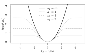
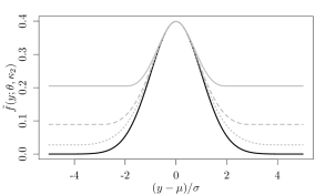
Figure 2.1: Squared-error loss and Tukey’s loss (left) and corresponding (improper) densities (right). The improper densities for Tukey’s loss are scaled to match the mode of the Gaussian density.

Setting $\kappa_{2}$ in Tukey’s loss is related to the so-called robustness-efficiency trade-off, an issue that has been unsettled for at least 60 years; see box1953non and tukey1960survey. While $\kappa_{2}=\infty$ gives the most efficient parameter estimates if the data are Gaussian, they are least robust outliers. Decreasing $\kappa_{2}$ increases robustness, but can significantly reduce estimation efficiency if $\kappa_{2}$ is set too small. We address this issue by learning from the data whether or not to estimate parameters in a robust fashion, i.e. selecting between $\ell_{1}$ and $\ell_{2}$, and estimating $\kappa_{2}$ when $\ell_{2}$ is chosen. We remark that the estimated $\kappa_{2}$ does not attempt to provide an optimal robustness-efficiency trade-off in the sense of minimising estimation error under an arbitrary data-generating $g(y)$. Rather, it seeks to define a predictive distribution on $y$ that portrays its nature accurately, in terms of infinitesimal relative probabilities (Section 3). This said, our method attains a good robustness-efficiency trade-off in our examples. Also, per our model selection consistency results, if data are truly Gaussian (or nearly so) then our framework collapses to inference under the Gaussian model, leading to efficient estimates.

Despite the importance of the robustness-efficiency trade-off, we are aware of limited work setting $\kappa_{2}$ in a principled, data-driven manner. Rule-of-thumb methods are popular, e.g. setting “$\kappa_{2}=4.6851$, gives approximately 95% asymptotic efficiency of L2 minimization on the standard normal distribution of residuals” (belagiannis2015robust), setting $\kappa_{2}=1.547$ to obtain a breakdown of 1/2 (rousseeuw1984robust), or a balance of breakdown and efficiency (e.g. riani2014consistency). More formal approaches rely on estimating quantiles of the data (e.g. sinova2016tukey), minimising an estimate of parameter mean squared error (see li2021robust, who applied the method of warwick2005choosing to Tukey’s loss), or minimising the maximum change in parameter estimates resulting from perturbing one observation (li2021robust).

2.2.2 Non-parametric Kernel Density Estimation

Suppose that $y_{i}\sim g$ independently for $i=1,\ldots,n$ and one wishes to estimate $g$. The kernel density estimate at a given value $x$ is given by

$$\hat{g}_{h}(x)=\frac{1}{nh}\sum_{i=1}^{n}K\left(\frac{x-y_{i}}{h}\right)$$ (5)

where the kernel $K(\cdot)$ is a symmetric, finite variance probability density, and $h$ is the bandwidth parameter. For simplicity we focus on the Gaussian kernel $K(x)=N(x;0,1)$.

The bandwidth $h$ is an important parameter controlling the smoothness and accuracy of $\hat{g}_{h}$. Popular strategies to set the bandwidth are rule-of-thumb and plug-in methods (e.g. silverman1986density), cross-validation (habbema1974stepwise, robert1976choice) and minimising an estimate of integrated square error (rudemo1982empirical, bowman1984alternative).

Unfortunately, standard Bayesian inference cannot be used to learn $h$ from data. The reason is that although (5) defines a proper probability distribution for a future observation $x$, a Bayesian framework requires a proper model for the observed data given the parameter. In our notation, the model likelihood $f(y;\theta,\kappa)\propto\prod_{i=1}^{n}\hat{g}_{h}(y_{i})$ with $\theta=\emptyset$ and hyper-parameter $\kappa=\{h\}$ has an infinite normalising constant. To see this, note that

$$\hat{g}_{h}(y_{i})= \frac{1}{nh}\sum_{j=1}^{n}K\left(\frac{y_{i}-y_{j}}{h}\right)=\frac{1}{nh\sqrt{2\pi}}+\frac{1}{nh\sqrt{2\pi}}\sum_{j\neq i}^{n}\exp\left\{-\frac{(y_{i}-y_{j})^{2}}{2h^{2}}\right\},$$ (6)

where the first term integrates to infinity with respect to $y_{i}$. Hence, (5) illustrates a situation where one has an ‘algorithm’ for producing a density estimate for future observations that defines an improper probability model for the observed data.

2.3 The failure of standard technology

As we discussed a main challenge is that standard tools are not, in general, applicable to compare improper models. Another challenge occurs when one wishes to estimate a hyperparameter $\kappa_{k}$ of a given improper model $k$, e.g. Tukey’s cut-off or the kernel bandwidth. For example, the general Bayesian might consider mimicking standard Bayes or marginal likelihood estimation by defining

$$\hat{\kappa}_{k}:=\arg\max_{\kappa_{k}\in\mathcal{K}}\int\pi_{k}(\theta_{k})\exp\{-\ell_{k}(y;\theta_{k},\kappa_{k})\}d\theta_{k}.$$ (7)

Unfortunately, such procedure often produces degenerate estimates. For example, from (4), it is clear that for fixed $\theta_{2}=\{\beta,\sigma^{2}\}$ Tukey’s loss is increasing in $\kappa_{2}$ and therefore (7) selects $\hat{\kappa}_{2}=0$ independently of the data. Similarly, in the kernel density estimation example (7) selects $h=0$ (habbema1974stepwise, robert1976choice).

2.4 Fisher’s divergence and the Hyvärinen score

hyvarinen2005estimation proposed a score matching approach for models with intractable normalising constants. Score matching minimises Fisher’s divergence to the data-generating $g(\cdot)$ in (1), that is

$$\theta_{k}^{\ast}: =\operatorname*{arg\,min}_{\theta_{k}\in\Theta_{k}}D_{F}(g(\cdot)||f_{k}(\cdot;\theta_{k}))=\operatorname*{arg\,min}_{\theta_{k}\in\Theta_{k}}\mathbb{E}_{z\sim g}\left[H(z;f_{k}(\cdot;\theta_{k}))\right],$$ (8)

where the right-hand side follows from integration by parts under minimal tail conditions, and

$$H(z;f_{k}(\cdot;\theta_{k})):=2\frac{\partial^{2}}{\partial z^{2}}\log f_{k}(z;\theta_{k})+\left(\frac{\partial}{\partial z}\log f_{k}(z;\theta_{k})\right)^{2},$$ (9)

is the Hyvärinen score ($\mathcal{H}$-score). As discussed we focus on univariate $z\in\mathbb{R}$, but (9) can be extended to multivariate $z=(z_{1},\ldots,z_{d})$ (hyvarinen2005estimation) via

$$H(z;f_{k}(\cdot;\theta_{k})):=2\sum_{j=1}^{d}\frac{\partial^{2}}{\partial z_{j}^{2}}\log f_{k}(z;\theta_{k})+\|\nabla_{z}\log f_{k}(z;\theta_{k})\|^{2}.$$ (10)

See also lyu2009interpretation for further options on extending score-matching to multivariate settings .

Given $y_{i}\sim g$ independently across $i=1,\ldots,n$ one can estimate $\theta_{k}^{*}$ by minimising

$$\hat{\theta}_{k}:=\operatorname*{arg\,min}_{\theta_{k}\in\Theta_{k}}\frac{1}{n}\sum_{i=1}^{n}H(y_{i};f_{k}(\cdot;\theta_{k}))$$ (11)

A critical feature for our purposes is that the $\mathcal{H}$-score depends only on the first and second derivatives of $\log f_{k}$ and hence the normalising constant does not play a role, independently of whether it is finite or not. Hence, unlike methods designed for intractable but finite normalisation constants, the $\mathcal{H}$-score is applicable to improper models. The $\mathcal{H}$-score enjoys desirable properties. For example, dawid2016minimum proved that $\hat{\theta}_{k}$ is consistent and asymptotically normal, and dawid2015bayesian, shao2019bayesian showed that its prequential application leads to consistent Bayesian model selection under improper priors.

Closest to our work, matsuda2019information proposed the score matching information criteria ( to select between models with intractable normalising constants. This criterion estimates Fisher’s divergence by correcting the in-sample Hyvärinen score by an estimate of its asymptotic bias. We emphasise two main distinctions with our work. The first is the extension to improper models. Second, these authors used cross-validations and predictive criteria similar to the AIC, which do not lead to consistent model selection, whereas we focus on structural learning where one seeks guarantees on recovering the loss that best approximates the data-generating $g$.

3 Inference for improper models

We now present our framework. Section 3.1 interprets an improper model in terms of relative probabilities and motivates Fisher’s divergence as a criterion to fit such a model. Section 3.2 proposes using the $\mathcal{H}$-score to define a general Bayesian posterior to learn hyper-parameters and choose among a collection of models, some or all of which may be improper. Section 3.3 proposes a Laplace approximation to the $\mathcal{H}$-Bayes factors, which we use both in our theoretical treatment and examples. Finally, Section 3.4 argues for using the $\mathcal{H}$-score within a two-step procedure: first selecting a model and estimating hyper-parameters using the $\mathcal{H}$-score, then reverting to standard general Bayes to learn the parameters of interest.

3.1 Inference through relative probabilities

Our goal is to select which model $f_{k}$ describes the data best, in terms of helping interpret the data-generating $g$. The main difficulty is that, since $f_{k}$ may be improper, it is unclear how to define “best”. Our strategy is to view $f_{k}$ as expressing relative probabilities, in contrast to the usual absolute probabilities. For example $f_{k}(y_{0},\theta_{k})/f_{k}(y_{1},\theta_{k})$ describes how much more likely is it to observe $y$ near $y_{0}$ than near $y_{1}$. As an illustration, consider Tukey’s loss in (4). For any pair $(y_{0},y_{1})$ such that $|y_{0}-x^{T}\beta|,|y_{1}-x^{T}\beta|<\kappa_{2}\sigma$ are small, Tukey’s loss is approximately equal to the squared loss, hence

$$\frac{f_{2}(y_{0};\theta_{2},\kappa_{2})}{f_{2}(y_{1};\theta_{2},\kappa_{2})}\approx\frac{\mathcal{N}\left(y_{0};x^{T}\beta,\sigma^{2}\right)}{\mathcal{N}\left(y_{1};x^{T}\beta,\sigma^{2}\right)}.$$ (12)

In contrast, for any pair such that $|y_{0}-x^{T}\beta|,|y_{1}-x^{T}\beta|>\kappa_{2}\sigma$ we have $\nicefrac{{f_{2}(y_{0},\theta_{2},\kappa_{2})}}{{f_{2}(y_{1},\theta_{2},\kappa_{2})}}=1$. That is, Tukey’s loss induces relative beliefs that observations near the mode behave like Gaussian variables, while all faraway observations are equally likely. This encodes the notion that one does not know much about the tails beyond their being thick, which is difficult to express using a proper probability distribution.

We argue that Fisher’s divergence is well-suited to evaluate how closely the relative probabilities of any such $f_{k}$ approximate those from $g$. Assuming that the gradients of $g(y)$ and $f_{k}(y)$ are finite for all $y$, Fisher’s divergence in (1) can be expressed as

$$D_{F}(g||f_{\theta}) =\int\left|\left|\lim_{\epsilon\rightarrow 0}\frac{\log\frac{g(y+\epsilon)}{g(y)}-\log\frac{f_{k}(y+\epsilon;\theta)}{f_{k}(y;\theta)}}{\epsilon}\right|\right|_{2}^{2}g(y)dy.$$ (13)

Therefore, minimising Fisher’s divergence (equivalently, the Hyvärinen score) targets a $f_{k}$ that approximates the relative probabilities of $g$ in an infinitesimal neighbourhood around $y$, in the quadratic error sense, on the average with respect to $g(y)$. This observation extends the usual motivation for the Hyvärinen score as a replacement of likelihood inference when the normalising constant is intractable to being a justifiable criteria to score improper models.

3.2 The $\mathcal{H}$-score

We consider a general Bayesian framework where the loss is defined by applying the $\mathcal{H}$-score to the density $f_{k}(y;\theta_{k},\kappa_{k})=\exp\{-\ell_{k}(y;\theta_{k},\kappa_{k})\}$, which gives the general posterior

$$\pi^{H}(\theta_{k},\kappa_{k}|y)\propto\pi_{k}(\theta_{k},\kappa_{k})\exp\left\{-\sum_{i=1}^{n}H(y_{i};f_{k}(\cdot;\theta_{k},\kappa_{k}))\right\}.$$ (14)

We refer to (14) as the $\mathcal{H}$-posterior, which is a particular case of the scoring rule posteriors of giummole2019objective. Note that (14) is different from the general Bayesian posterior directly associated to $\ell_{k}$ in (2). An important property of (14) is that it provides a consistent estimator for parameters $\theta_{k}$ and hyper-parameters $\kappa_{k}$. Specifically, Proposition 1 shows that, under regularity conditions, $\tilde{\eta}_{k}=(\tilde{\theta}_{k},\tilde{\kappa}_{k})$ maximising (14) recovers the optimal $\eta_{k}^{*}=(\theta_{k}^{*},\kappa_{k}^{*})$ according to Fisher’s divergence.

Proposition 1 requires mild regularity conditions A1-A3, discussed in Section LABEL:App:TechnicalConditions. Briefly, A1 requires continuous second derivatives of the Hyvärinen score, that it has a unique minimiser, and that its first derivative has finite variance. A2 requires that the Hyvärinen score is dominated by an integrable function, which can be easily seen to hold for Tukey’s loss, for example. Finally, A3 requires that the Hessian of the $\mathcal{H}$-score is positive and finite around $\eta_{k}^{\ast}$.

Proposition 1 extends hyvarinen2005estimation (Corollary 3), who stated that $\tilde{\eta}_{k}$ converges to $\eta_{k}^{*}$ in probability, to also give a $1/\sqrt{n}$ convergence rate. Another difference is that hyvarinen2005estimation considered the well-specified case where $g(y)=f_{k}(y;\theta_{k}^{\ast},\kappa_{k}^{\ast})$, which in particular requires $f_{k}$ to be a proper model. Proposition 1 also extends dawid2016minimum (Theorem 2), who proved asymptotic normality for $\mathcal{H}$-score based estimators. Said asymptotic normality does in general not hold when $\eta_{k}^{\ast}$ lies on the boundary of the parameter space, e.g. for Tukey’s loss if the data are truly Gaussian then $\kappa^{\ast}_{2}=\infty$. By Proposition 1, even if normality does not hold, one still attains $\sqrt{n}$ consistency to estimate $\kappa_{2}^{*}$. In terms of technical conditions, dawid2016minimum do not list them but refer to standard M-estimation theory assumptions, see Theorem 5.23 in van2000asymptotic. These are similar to our assumptions and include differentiability and Lipschitz conditions in $\eta_{k}$, the existence of a second order Taylor expansion around $\eta_{k}^{*}$, and a non-singular Hessian at $\eta_{k}^{*}$. The main differences are that we require twice differentiability in $y$ and $\eta_{k}$, and that we consider a compact parameter space to allow for boundary parameter values (e.g. $1/\kappa_{2}^{*}=0$ for Tukey’s loss, after a re-parameterisation discussed in Section 4). Further, Proposition 1 extends previous results by explicitly considering improper models and the learning of their hyperparameters.

As is standard under model misspecification, the shape of the $\mathcal{H}$-posterior does not match the frequentist distribution of the posterior mode $\tilde{\eta}_{k}=(\tilde{\theta}_{k},\tilde{\kappa}_{k})$ (giummole2019objective), i.e. it does not have valid frequentist coverage. Per Proposition 1 and Theorem 1 this is not a major issue for selecting a loss $k$ and hyper-parameters $\kappa_{k}$, which is our main focus. However, posterior inference on $\theta_{k}$ under the selected $(k,\kappa_{k})$ should be properly calibrated, as we discuss in Section 3.4.

Proposition 1.

Let $y=(y_{1},\ldots,y_{n})\sim g$, $\tilde{\eta}_{k}=(\tilde{\theta}_{k},\tilde{\kappa}_{k})$ maximise (14), and $\eta_{k}^{*}=(\theta_{k}^{*},\kappa_{k}^{*})$ minimise Fisher’s divergence from $f_{k}(\theta_{k},\kappa_{k})$ to $g$. Assume Conditions A1-A2 in Section LABEL:App:TechnicalConditions. Then, as $n\rightarrow\infty$,

$$\left|\left|\tilde{\eta}_{k}-\eta_{k}^{\ast}\right|\right|_{2}=o_{p}(1),$$

where $||\cdot||_{2}$ is the $L_{2}$-norm. Further, if Condition A3 also holds, then

$$\left|\left|\tilde{\eta}_{k}-\eta_{k}^{\ast}\right|\right|_{2}=O_{p}(\nicefrac{{1}}{{\sqrt{n}}}).$$

A consequence of Proposition 1 is that one can use (14) to learn tempering hyper-parameters. Specifically, suppose that one considers a family of losses $w_{k}\ell_{k}()$, where $w_{k}>0$ is a tempering parameter. While $w_{k}$ does not affect the point estimate of $\theta_{k}$ given by (2), it plays an important role in driving the posterior uncertainty on $\theta_{k}$. Within our framework, one may define

$$f_{k}(y;\theta_{k},\kappa_{k}^{\prime})=\exp\{-\ell_{k}^{\prime}(y;\theta_{k},\kappa_{k}^{\prime})\}=\exp\{-w_{k}\ell_{k}(y;\theta_{k},\kappa_{k})\}$$

where $\kappa_{k}^{\prime}=(\kappa_{k},w_{k})$ and $\ell_{k}^{\prime}()=w_{k}\ell_{k}()$. By Proposition 1, one can consistently learn the Fisher-divergence optimal $\kappa_{k}^{\prime}$, and in particular $w_{k}$. In contrast, in the general Bayes posterior (2) it is challenging to estimate such $w_{k}$. Current strategies to set $w_{k}$ are optimising an upper-bound on generalisation error in PAC-Bayes (catoni2007pac), estimating $w_{k}$ via marginalisation similar to the “Safe Bayesian” fractional likelihood approach of grunwald2012safe, or using information theoretic arguments to calibrate $w_{k}$ to match certain limiting sampling distributions (holmes2017assigning, lyddon2019general). These strategies essentially view $w_{k}$ as a tuning parameter. In contrast, in our framework $w_{k}$ is viewed as a parameter of interest that controls the dispersion of the improper model and affects its interpretation. See Section LABEL:Sec:KDE for an illustration in kernel density estimation.

Recall that our main goal is model comparison. To this end, in analogy to the marginal likelihood in standard Bayesian model selection, we define the integrated $\mathcal{H}$-score

$$\mathcal{H}_{k}(y)=\int\pi_{k}(\theta_{k},\kappa_{k})\exp\left\{-\sum_{i=1}^{n}H(y_{i};f_{k}(\cdot;\theta_{k},\kappa_{k}))\right\}d\theta_{k}d\kappa_{k}.$$ (15)

Also, analogously to Bayes factors and posterior model probabilities, we define the $\mathcal{H}$-Bayes factor as $B^{(\mathcal{H})}_{kl}:=\mathcal{H}_{k}(y)/\mathcal{H}_{l}(y)$ and

$$\pi(k\mid y)=\frac{\mathcal{H}_{k}(y)\pi(k)}{\sum_{l}\mathcal{H}_{l}(y)\pi(l)}=\left(1+\sum_{l\neq k}B^{(\mathcal{H})}_{lk}\frac{\pi(l)}{\pi(k)}\right)^{-1},$$ (16)

where $\pi(k)$ is a given prior probability for each model $k$. In our examples we use uniform $\pi(k)$, since we focus on the comparison of a few models, but in high-dimensional settings it may be desirable to set $\pi(k)$ to favour simpler models.

We note that an interesting alternative strategy for model comparison, also based on the $\mathcal{H}$-score, is to extend the prequential framework of dawid2015bayesian and shao2019bayesian designed for improper priors. Therein one could adopt a general Bayesian framework, replacing the likelihood by $f_{k}(x_{i};\theta_{k},\kappa_{k})=\exp\{-\ell_{k}(x_{i};\theta_{k}\kappa_{k})\}$. Prequential approaches enjoy desirable properties, such as consistency and leading to joint coherent inference on the model and parameter values. Unfortunately, prequential inference is computationally hard, particularly when considering several models. First, for each model inference needs to be updated $n$ times to calculate the one-step-ahead predictive distribution. Second, said updates are not permutation invariant, so one should in principle consider the $n!$ orderings of the data. Thus, while interesting, we leave such line of research for future work. We remark however that a salient feature in dawid2015bayesian is that one may use improper priors. In contrast, our framework requires one to use proper priors. The reason is that otherwise one may suffer the usual Jeffreys-Lindley paradox in Bayesian model selection (lindley1957statistical). Specifically, if one considers two nested models and sets an improper prior under the larger one, then our $\mathcal{H}$-Bayes factor in favor of the smaller model is infinite, i.e. one selects the smaller model regardless of the data.

3.3 Laplace approximation and BIC-type criterion

There are many available strategies to compute or estimate integrals such as $\mathcal{H}_{k}(y)$ in (15) (see llorente2020marginal for a review). For its speed and analytic tractability, we consider the Laplace approximation

$$\tilde{\mathcal{H}}_{k}(y): =(2\pi)^{\frac{d_{k}}{2}}\pi_{k}\left(\tilde{\eta}_{k}\right)\exp\left\{-\sum_{i=1}^{n}H\left(y_{i};f_{k}\left(\cdot;\tilde{\eta}_{k}\right)\right)\right\}|A_{k}\left(\tilde{\eta}_{j}\right)|^{-\frac{1}{2}},$$ (17)

$$\textrm{ with }\tilde{\eta}_{k}: =\operatorname*{arg\,min}_{\eta_{k}}\sum_{i=1}^{n}H(y_{i};f_{k}(\cdot;\eta_{k}))-\log\pi_{k}(\eta_{k}),$$ (18)

being the mode of the log $\mathcal{H}$-posterior, $A_{k}\left(\eta_{k}\right)$ its Hessian at $\eta_{k}$, and $\eta_{k}=(\theta_{k},\kappa_{k})$. We denote the corresponding Laplace approximate $\mathcal{H}$-Bayes-factor by $\tilde{B}^{(\mathcal{H})}_{kl}:=\mathcal{H}_{k}(y)/\mathcal{H}_{l}(y)$.

Computational tractability is important when one considers many models or the integrand is expensive to evaluate, e.g. in our kernel density examples it requires $\mathcal{O}(n^{2})$ operations. Further, the availability of a closed-form expression facilitates its theoretical study (Section 4). See kass1990validity for results on the validity of Laplace approximations. We do not undertake such a study, instead we prove our results directly for the approximation (17) that we actually use for inference.

Although we motivate our methodology from a Bayesian standpoint, we note that $\tilde{\mathcal{H}}_{k}(y)$ can be viewed as Bayesian-inspired information criteria analogous to the BIC (schwarz1978estimating). Specifically, in regular settings where $A_{k}$ is of order $1/n$, one could take the leading terms in $\log\tilde{\mathcal{H}}_{k}(y)$ to obtain

$$-\sum_{i=1}^{n}H\left(y_{i};f_{k}(\cdot;\tilde{\eta}_{k})\right)-\frac{d_{k}}{2}\log(n)+\log\pi_{k}\left(\tilde{\eta}_{j}\right)$$

as a model selection criterion. This expression is analogous to the BIC, except for the log prior density term, which converges to a constant for any $\pi_{k}$ bounded away from 0 and infinity. The log prior term can play a relevant role however when considering non-local priors where $\pi_{k}(\eta_{k})$ can be equal to 0 for certain $\eta_{k}$, see Section 4.

3.4 Two-step inference and model averaging

As discussed the $\mathcal{H}$-posterior (14) asymptotically recovers the parameters $(\theta_{k}^{\ast},\kappa_{k}^{\ast})$ minimising Fisher’s divergence, whereas the general Bayesian posterior (2) recovers the parameters minimising the expected loss $\tilde{\theta}_{k}^{\ast}=\operatorname*{arg\,min}_{\theta_{k}\in\Theta_{k}}\int\ell_{k}(y;\theta_{k},\kappa_{k})g(y)dy$, for a given $\kappa_{k}$.

We adopt the pragmatic view that, while one may consider the $\mathcal{H}$-posterior to choose a model $k$ and learn the associated hyper-parameter $\kappa_{k}$, after said choice one may want to obtain standard inference under the selected model. That is, one desires to learn

$$\arg\min_{\theta_{k}\in\Theta_{k}}\int\ell_{k}(y;\theta_{k},\kappa_{k}^{\ast})g(y)dy.$$ (19)

For example, suppose that the $\mathcal{H}$-score selects a proper probability model (e.g. the Gaussian model). One may then wish that inference collapses to standard Bayesian inference under that model, rather than being based on the $\mathcal{H}$-posterior in (14). This is easily achieved with a two-step procedure. First, one uses (16) to select $\hat{k}$ and (14) to estimate $\hat{\kappa}_{\hat{k}}$. Second, given $(\hat{k},\hat{\kappa}_{\hat{k}})$ one uses the general Bayesian posterior (2) for $\theta_{\hat{k}}$. A further alternative to selecting a single model is to mimic Bayesian model averaging (hoeting1999bayesian), where the estimates under each model are weighted according to the posterior probabilities in (16).

As an important point for quantifying uncertainty on $\theta_{k}$, if the data-generating $g(y)$ is not contained in any of the considered models, the generalized posterior $\pi_{k}(\theta_{k}\mid y,\kappa_{k})\propto\exp\{-\ell_{k}(y;\theta_{k},\kappa_{k})\}\pi_{k}(\theta_{k}\mid\kappa_{k})$ in (2) is miss-calibrated relative to the sampling distribution of its posterior mode $\tilde{\theta}_{k}$. This issue is not specific to generalized posteriors, it also affects any standard Bayesian posterior when the model is misspecified. When the posterior is asymptotically normal, it is possible to define a calibrated version that provides valid frequentist uncertainty quantification. Briefly, following ribatet2012bayesian and giummole2019objective, define the calibrated posterior as

$$\pi_{k}^{C}(\theta_{k}\mid y,\kappa_{k})=\pi_{k}(\tilde{\theta}_{k}+C(\theta_{k}-\tilde{\theta}_{k})\mid y,\kappa_{k}),$$

where $C$ is any matrix satisfying $C^{T}J_{k}C=J_{k}K_{k}^{-1}J_{k}$, $J_{k}$ is the expected Hessian of $-\ell_{k}$ and $K_{k}$ the covariance of its gradient, evaluated at $\tilde{\theta}^{*}_{k}$ (in practice, at its estimate $\tilde{\theta}_{k}$). It is easy to check that $\pi_{k}^{C}$ has the same mode as $\pi_{k}$. Specifically, one may take $C=J_{k}^{-1/2}\Sigma^{1/2}$, where $\Sigma=J_{k}K_{k}^{-1}J_{k}$ (ribatet2012bayesian, Section 2.2). Then, the shape of the calibrated posterior $\pi^{C}_{k}$ at $\theta^{*}_{k}$ asymptotically matches the sampling distribution of $\tilde{\theta}_{k}$, and hence provides valid uncertainty quantification (giummole2019objective, Theorem 3.1).

4 Consistency of $\mathcal{H}$-score model selection

We now state Theorem 1, our main result that (17) consistently selects the model closest in Fisher’s divergence to the data-generating $g$. When several models attain the same minimum, as may happen when considering nested models, then (17) selects that of smallest dimension. The proof does not require that the Hyvärinen score is asymptotically normal, which holds under the conditions in Theorem 2 of dawid2016minimum, but simply the $\sqrt{n}$-consistency proven in Proposition 1.

Theorem 1 mirrors standard results for Bayes factors (Theorem 1 in dawid2011posterior), the main difference being that it involves Fisher’s rather than Kullback-Leibler divergence. As discussed after the theorem, when the optimal hyper-parameter occurs at the boundary the model selection consistency provided by Theorem 1 may not hold, unless one uses a suitable adjustment. Before stating the theorem, we interpret its implications. Part (i) considers a situation where one compares two models $l$ and $k$ such that the former is closer to $g$ in Fisher’s divergence. Then $\tilde{B}^{(\mathcal{H})}_{kl}$ converges to 0 at an exponential rate in $n$. Part (ii) considers that both models attain the same Fisher’s divergence, e.g. nested models such as Tukey’s and the Gaussian model when the data are truly Normal. Then, $\tilde{B}^{(\mathcal{H})}_{kl}$ favours the smaller model at a polynomial rate in $n$.

dawid2015bayesian also proved model selection consistency for a prequential application of the $\mathcal{H}$-score (which differs from our methodology), restricted to well-specified linear regression models. shao2019bayesian extended the results to other models but only considered non-nested comparisons, for nested cases only a conjecture is given. Similarly to us they require twice differentiability, Lipschitz conditions on the score and H-score functions, but other assumptions are stronger. For example, the posterior is assumed to concentrate on the optimal $\eta_{k}^{*}$ (we prove such result) and must have certain bounded posterior expectations in supremum norm.

Theorem 1.

Assume Conditions A1-A4, and let $\eta_{k}^{*}=(\theta_{k}^{*},\kappa_{k}^{*})$ be as in Proposition 1.

1. Suppose that $\mathbb{E}_{g}[H(y;f_{l}(\cdot;\eta^{\ast}_{l}))]<\mathbb{E}_{g}[H(y;f_{k}(\cdot;\eta^{\ast}_{k}))]$. Then

   $$\frac{1}{n}\log\tilde{B}^{(\mathcal{H})}_{kl}=\mathbb{E}_{g}[H(y;f_{l}(\cdot;\eta^{\ast}_{l}))]-\mathbb{E}_{g}[H(y;f_{k}(\cdot;\eta^{\ast}_{k}))]+o_{p}(1).$$

2. Suppose that $\mathbb{E}_{g}[H(y;f_{l}(\cdot;\eta^{\ast}_{l}))]=\mathbb{E}_{g}[H(y;f_{k}(\cdot;\eta^{\ast}_{k}))]$. Then

   $$\log\tilde{B}^{(\mathcal{H})}_{kl}=\frac{d_{l}-d_{k}}{2}\log(n)+O_{p}(1).$$

The result requires Conditions A1-A4 given and discussed in Section LABEL:App:TechnicalConditions. Conditions A1-A3 are mild and also summarised before Proposition 1, whereas A4 imposes a Lipschitz condition on the $\mathcal{H}$-score and its Hessian. As an important remark, the slower rate in Part (ii) is due to Condition A1 that the prior density $\pi_{l}(\eta_{l}^{*})>0$ at the optimal $\eta_{l}^{*}$, where $l$ is the larger model. This defines a so-called local prior, in contrast to non-local priors (johnson2012bayesian, rossell2017nonlocal) which place zero density at the value $\kappa_{l\setminus k}^{*}$ where the more complicated model $l$ recovers the simpler model $k$. Since non-local priors violate A1, Corollary LABEL:Thm:HscoreConsistencyNLPs extends Theorem 1 to show that non-local priors attain faster rates in Part (ii), while maintaining the exponential rates in Part (i). We will demonstrate that this improvement can have non-negligible practical implications in Section 5.2.

Another practically-relevant remark is that A3 requires a finite expected Hessian near the optimal $(\theta_{k}^{*},\kappa_{k}^{*})$, which can be problematic in certain settings. For example, in Tukey’s loss if data are truly Gaussian then $\kappa_{2}^{*}=\infty$, which leads to an infinite Hessian. For Tukey’s loss the problem can be avoided by reparameterising $\nu_{2}=1/\kappa_{2}^{2}$, for which the Hessian is finite, but more generally such a reparameterisation may not be obvious or not exist. These cases provide a further use for non-local priors. By Corollary LABEL:Thm:HscoreConsistencyNLPs, one may set a non-local prior that vanishes sufficiently fast at the boundary (basically, a faster rate than that at which the Hessian diverges) to attain model selection consistency.

As a final remark, we also prove that under extended Conditions A1-A7 the score matching information criterion of matsuda2019information does not lead to consistent model selection for the nested setting in Part (ii), see Corollary LABEL:Thm:SMICConsistency. This result is analogous to predictive criteria such as cross-validation or Akaike’s information criterion not leading to consistent model selection, see shao1997asymptotic.

5 Robust Regression with Tukey’s loss

We revisit the robust regression in Section 2.2, where one considers a Gaussian model and the improper model defined by Tukey’s loss. Section 5.1 illustrates that when the data contain outliers, the $\mathcal{H}$-score chooses Tukey’s model and learns its cut-off hyper-parameter in a manner that leads to robust estimation. Section 5.2 shows the opposite situation, where data are truly Gaussian, and the benefits of setting a non-local prior on Tukey’s cut-off hyper-parameter to improve the model selection consistency rate. Finally, Section 5.3 shows two gene expression datasets, one exhibiting Gaussian behavior and the other thicker tails. We compare our results to the matsuda2019information which, despite not being designed to compare improper models, to our knowledge is the only existing criterion that can be used for this task.

The $\mathcal{H}$-scores for the squared loss ($\ell_{1}$) and Tukey’s loss ($\ell_{2}$) (see Section LABEL:App:HscoreGaussianTukeys) are

$$H_{1}(y;f(\cdot;x,\theta_{1})) =\sum_{i=1}^{n}-\frac{2}{\sigma^{2}}+\frac{(y_{i}-x_{i}^{T}\beta)^{2}}{\sigma^{4}}$$ (20)

$$H_{2}(y;f(\cdot;x,\theta_{2},\kappa_{2})) =\sum_{|y_{i}-x_{i}^{T}\beta|\leq\kappa_{2}\sigma}\left\{\left(\frac{(y_{i}-x_{i}^{T}\beta)}{\sigma^{2}}-\frac{2(y_{i}-x_{i}^{T}\beta)^{3}}{\kappa_{2}^{2}\sigma^{4}}+\frac{(y_{i}-x_{i}^{T}\beta)^{5}}{\kappa_{2}^{4}\sigma^{6}}\right)^{2}-\right.$$

$$\qquad\qquad\qquad\left.2\left(\frac{1}{\sigma^{2}}-\frac{6(y_{i}-x_{i}^{T}\beta)^{2}}{\kappa_{2}^{2}\sigma^{4}}+\frac{5(y_{i}-x_{i}^{T}\beta)^{4}}{\kappa_{2}^{4}\sigma^{6}}\right)\right\}.$$ (21)

Given our interest in learning $\kappa_{2}$, it is important to remark that its role is to define the proportion of observations that should be viewed as outliers. Thus, too small $\kappa_{2}$ leads to problems. First, minimising $H_{2}$ in (21) has a trivial degenerate solution by setting $(\beta,\sigma,\kappa_{2})$ where $\kappa_{2}$ is so small that only one observation satisfies $|y_{i}-x_{i}^{T}\beta|\leq\kappa_{2}\sigma$, and $y_{i}=x_{i}^{T}\beta$ for that observation. Such solution is undesirable, as it views all observations but one as outliers. Fortunately, it is possible to define a range of reasonable $\kappa_{2}$ using the notion of the breakdown point, i.e. the number of observations that can be perturbed without causing arbitrary changes to an estimator. Following rousseeuw1984robust, this leads to a constraint on $(\beta,\sigma,\kappa_{2})$ such that

$$\frac{1}{\rho(\kappa_{2},\kappa_{2})}\sum_{i=1}^{n}\rho\left(\frac{y_{i}-x_{i}^{T}\beta}{\sigma},\kappa_{2}\right)\leq\frac{n}{2}-p,$$ (22)

where $\rho\left(\frac{y_{i}-x_{i}^{T}\beta}{\sigma},\kappa_{2}\right)=\ell_{2}(y_{i};x_{i},\theta_{2},\kappa_{2})-\frac{1}{2}\log(2\pi\sigma^{2})$, $\ell_{2}$ is as in (4), and $p=\mbox{dim}(x_{i})$. See Section LABEL:App:TukeysBreakdown for the derivation and further discussion.

Regarding priors, throughout we set $\sigma^{2}\sim\mathcal{IG}(2,0.5)$ and $\beta|\sigma^{2}\sim\mathcal{N}\left(0,5\sigma^{2}I\right)$ for the Gaussian and Tukey models, in the latter case truncated to satisfy (22). The idea is that these are mildly informative priors, e.g. the prior variance of $\sigma^{2}$ is infinite, but avoid degenerate solutions by truncating using (22). For $\kappa_{2}$ we set an inverse gamma prior in terms of $\nu_{2}=1/\kappa_{2}^{2}$, $\pi_{2}^{\lx@acro@@@def{\smaller NLP}{\smaller NLP}{}{{\smaller NLP}}{{}}}(\nu_{2})=\mathcal{IG}(\nu_{2};a_{0},b_{0})$. The inverse gamma is a non-local prior (i.e. has vanishing density at $\nu_{2}=0$), which as discussed in Section 5.2 carries important benefits for model selection. Its prior parameters $(a_{0},b_{0})=(4.35,1.56)$ are set such that $P(\kappa_{2}\in(1,3))=0.95$. The reasoning is that one assigns high prior probability to the cutoff being in a reasonable default range, between 1-$\sigma$ and 3-$\sigma$. If data were truly Gaussian, 0.3% would lie outside the 3-$\sigma$ region and 68.3% within 1-$\sigma$. Hence, $\kappa_{2}=3$ would exclude clear outliers under the Gaussian, and $\kappa_{2}=1$ would keep most of the Gaussian data. We remark that this is a mildly informative prior, when warranted by the data the posterior can concentrate on $\kappa_{2}\not\in[1,3]$ outside this interval (e.g. for the DLD data in Section 5.3 the posterior mode was $\hat{\kappa}_{2}=4.12$). See Section LABEL:App:NLPSpecification for further discussion.

Finally, to satisfy the differentiability conditions of Theorem 1 and enable the use of standard second order optimisation software, we implemented a differentiable approximation to the indicator function in Tukey’s loss (see Section LABEL:App:AbsApprox).

5.1 The marginal $\mathcal{H}$-score in $\kappa$

Our first example illustrates the properties of the $\mathcal{H}$-score for calibrating the robustness-efficiency trade-off, in a setting where the data contain outliers. We simulated $n=500$ observations from the data-generating $g(y)=0.9\mathcal{N}(y;0,1)+0.1\mathcal{N}(y;5,3)$. The goal is to estimate the parameters of the larger component (uncontaminated data), in a manner that is robust to the presence of data from the smaller component (outliers). We compare the estimation from the Gaussian model $f_{1}$, which is correctly specified for 90% of the data, with that of the robust improper model arising from Tukey’s loss $f_{2}$ (where $x_{i}=1$ contains only the intercept term).

A first question of interest is studying the ability of the $\mathcal{H}$-score to learn the cutoff hyper-parameter $\kappa_{2}$. To this end, we measured the evidence for different $\kappa_{2}$ provided by the marginal $\mathcal{H}$-score

$$\mathcal{H}_{2}(y;\kappa_{2})=\int\pi_{2}(\theta_{2})\exp\left(-\sum_{i=1}^{n}H(y_{i};f_{2}(\cdot;\theta_{2},\kappa_{2}))\right)d\theta_{2}.$$ (23)

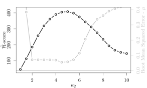
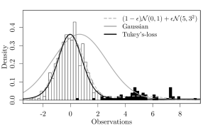
Figure 5.1: Left: Marginal $\mathcal{H}$-score $\mathcal{H}_{2}(y;\kappa_{2})$ (black) and asymptotic approximation to the RMSE of $\hat{\beta}(\kappa_{2})$ (grey) for several $\kappa_{2}$. Right: Histogram of $n=500$ observations from $g(y)=0.9\mathcal{N}(y;0,1)+0.1\mathcal{N}(y;5,3)$ and fitted Gaussian and Tukey ($\hat{\kappa}_{2}=5$) models (height set to match the mode of $g(y)$).

The left panel in Figure 5.1 shows $\mathcal{H}_{2}(y;\kappa_{2})$ (black line) for a grid $\kappa_{2}\in\{1,1.5,2,\ldots,10\}$, along with an asymptotic approximation to the root mean squared error (RMSE) of $\hat{\beta}(\kappa_{2})$ motivated by warwick2005choosing (see Section LABEL:App:asympt_MSE). The marginal $\mathcal{H}$-score is highest for $\hat{\kappa}_{2}=5$, i.e. this value is chosen as best approximating the data-generating $g$. The right panel of Figure 5.1 shows that Tukey’s model for $\hat{\kappa}_{2}=5$ provides a good description of the uncontaminated component of the data, in the sense of capturing the log-gradient of $g(y)$ around the mode, and excludes most outliers.

Interestingly, the RMSE associated to $\hat{\beta}(\kappa_{2})$ at $\hat{\kappa}_{2}=5$ was close to optimal (Figure 5.1, grey line). A convenient feature of the asymptotic RMSE is that we can examine the decomposed effect of the bias (due to contamination) and the variance, see Section LABEL:App:asympt_MSE for details. For too small $\kappa_{2}$ the RMSE increases, since then there are more observations beyond the cutoff (viewed as outliers), increasing the variance of $\hat{\beta}(\kappa_{2})$. If $\kappa_{2}$ is too large, then the contaminated observations lie within the cutoff, which increases the bias (recall that at $\kappa_{2}=\infty$, $\hat{\beta}(\kappa_{2})$ is the sample mean).

5.2 Non-local priors and model selection consistency

We demonstrate the selection consistency (Theorem 1) when data are truly Gaussian, and that setting a non-local prior on the cutoff hyper-parameter $\kappa_{2}$ speeds up this selection (Corollary LABEL:Thm:HscoreConsistencyNLPs). We simulated $100$ independent data sets of sizes $n=100$, $1,000$, $10,000$ and $100,000$ from the data-generating $g(y_{i})=\mathcal{N}\left(y_{i};x_{i}^{T}\beta,\sigma^{2}\right)$, where the first entry in $x_{i}\in\mathbb{R}^{6}$ corresponds to the intercept and the remaining entries are Gaussian with unit variances and 0.5 pairwise covariances, $\beta=(0,0.5,1,1.5,0,0)$ and $\sigma^{2}=1$.

Recall that Tukey’s loss collapses to the Gaussian model for $\kappa_{2}=\infty$, and otherwise adds certain flexibility by allowing one to consider an improper model. If this extra flexibility is not needed, following Occam’s razor one wants to choose the Gaussian model. While Theorem 1 guarantees this to occur asymptotically, our experiments show that setting a local prior on $\kappa_{2}$ leads to poor performance, even for $n=100,000$. Specifically, we compare our default non-local prior $\pi_{2}^{\lx@acro@@@def{\smaller NLP}{\smaller NLP}{}{{\smaller NLP}}{{}}}(\nu_{2})=\mathcal{IG}(\nu_{2};4.35,1.56)$ to a (local) half-Gaussian prior $\pi_{2}^{\lx@acro@@@def{\smaller LP}{\smaller LP}{}{{\smaller LP}}{{}}}(\nu_{2})\propto 1_{\nu_{2}\geq 0}\mathcal{N}(\nu_{2};0,1)$, where $\nu_{2}=1/\kappa_{2}^{2}$. By Corollary LABEL:Thm:HscoreConsistencyNLPsIG, the log-$\mathcal{H}$-Bayes factor under the non-local prior should favor the Gaussian model at least at a $\sqrt{n}$ rate, in contrast to the local prior’s $\log(n)$ rate.

Figure 5.2 compares the ith our integrated $\mathcal{H}$-score under the local and non-local priors. Score differences are plotted such that negative values indicate correctly selecting the Gaussian model. Firstly, there is no evidence of eing consistent as $n$ grows, even for $n=100,000$ the wrong model was selected $11\%$ of the time. The $\mathcal{H}$-score under the local prior has a decreasing median in $n$, but exhibits heavy tails and even for $n=100,000$ it also failed to select the Gaussian model $11\%$ of the time. Under the non-local prior, already for $n=1,000$ the correct decision was made 99% of the time. These experiments illustrate the benefits of non-local priors to penalise parameter values near the boundary ($1/\kappa_{2}^{2}=0$, in this example). Recall also that, as discussed in Section 4, in general in such situations a local prior need not even attain consistency.

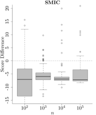
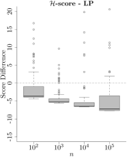
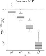
Figure 5.2: Selecting between the Gaussian and Tukey models in 100 truly Gaussian datasets. $\lx@acro@@@def{\smaller SMIC}{\smaller SMIC}{}{{\smaller SMIC}}{{}1(y)-\lx@acro@@@def{\smaller SMIC}{\smaller SMIC}{}{{\smaller SMIC}}{{}2(y)}}$) vs $\mathcal{H}$-score with local and non-local priors ($\log\tilde{\mathcal{H}}_{2}(y)-\log\tilde{\mathcal{H}}_{1}(y)$). Negative values correctly select the Gaussian model.

5.3 Real datasets

We considered two gene expression data sets from rossell2018tractable. In the first, the data are well-approximated by a Gaussian distribution, whereas the second exhibits thicker tails. In both examples we used the $\mathcal{H}$-score to compare the Gaussian model ($\ell_{1}$) and Tukey’s loss ($\ell_{2}$).

5.3.1 ata

The dataset from calon2012dependency concerns gene expression data for $n=262$ colon cancer patients. Previous work (rossell2017nonlocal, rossell2018tractable) focused on selecting genes that have an effect on the expression levels of a gene known to play an important role in colon cancer progression. Instead, we study the relation between nd the 7 genes (listed in Section LABEL:App:SelectedVariables) that appear in the ‘ pathway’ according to the KEGGREST package in R (tenenbaum2016keggrest), so that $p=8$ after including the intercept.

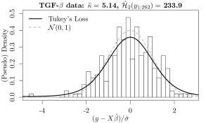
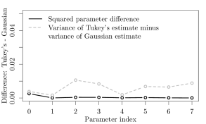
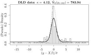
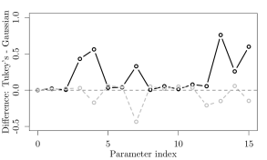
Figure 5.3: Top: ata, where the $\mathcal{H}$-score selected the Gaussian model. Bottom: ata, where the $\mathcal{H}$-score selected Tukey’s loss. Left: fitted Tukey-based density to the residuals. Right: Squared difference between the $\mathcal{H}$-posterior mean estimates of each $\beta_{j}$ under Tukey’s model minus that under the Gaussian (solid black line), and difference between their variances (estimated with $B=500$ bootstrap re-samples).

The top panels in Figure 5.3 summarises the results. The integrated $\mathcal{H}$-score for the Gaussian model was $\tilde{\mathcal{H}}_{1}(y)=272.88$ and that for Tukey’s loss $\tilde{\mathcal{H}}_{2}(y)=233.90$, providing strong evidence for the Gaussian model. This is in agreement with the $\lx@acro@@@def{\smaller SMIC}{\smaller SMIC}{}{{\smaller SMIC}}{{}1(y)=-283.93}$ and $\lx@acro@@@def{\smaller SMIC}{\smaller SMIC}{}{{\smaller SMIC}}{{}2(y)=-277.55}$, where minimisation is desired) and results in rossell2018tractable, who found evidence for Gaussian over (thicker) Laplace tails. The left panel shows the fitted densities which, in conjunction with the Q-Q Normal plots in Figure LABEL:Fig:TGFB_DLD_Gaussian_results, show that the residual distribution is well-approximated by a Gaussian. The right panel shows the squared difference between the $\mathcal{H}$-posterior mean parameter estimates of each $\beta_{j}$ under Tukey’s model minus that under the Gaussian, and the differences between their sampling variances (estimated via bootstrap, dashed gray line). Both models returned very similar point estimates, but the Gaussian had smaller variance for all parameters. Altogether, these results strongly support that the Gaussian model should be selected over Tukey’s.

5.3.2 ataset

We consider an RNA-sequencing data set from yuan2016plasma measuring gene expression for $n=192$ patients with different types of cancer. rossell2018tractable studied the impact of 57 predictors on the expression of a gene that can perform several functions such as metabolism regulation. To illustrate our methodology, we selected the 15 variables with the 5 highest loadings in the first 3 principal components, and used the integrated $\mathcal{H}$-score to choose between the Gaussian and Tukey’s loss. Section LABEL:App:SelectedVariables lists the selected variables.

The bottom panels of Figure 5.3 summarise the results. The $\mathcal{H}$-score strongly supported Tukey’s loss ($\tilde{\mathcal{H}}_{1}(y)=155.57$ for the Gaussian model, $\tilde{\mathcal{H}}_{2}(y)=783.94$ for Tukey’s), with $\mathcal{H}$-posterior mean estimate $\hat{\kappa}_{2}=4.12$. Indeed, the bottom left panel indicates that the residuals have thicker-than-Gaussian tails, see also the Q-Q Normal residual plot in Figure LABEL:Fig:TGFB_DLD_Gaussian_results. The bottom right panel illustrates two things. Firstly, the estimated coefficients of 6 of the 16 predictors differ quite considerably between the Gaussian model and Tukey’s loss (solid line). Second, the latter often have smaller variance (estimated via bootstrap). Both observations align with the presence of thicker-than-normal tails, which can cause parameter estimation biases and inflated variance. Notably, the $\mathcal{H}$-score agrees with rossell2018tractable, who selected Laplace over Gaussian tails, but disagrees with the $\lx@acro@@@def{\smaller SMIC}{\smaller SMIC}{}{{\smaller SMIC}}{{}1(y_{1:192})=-145.72}$ and $$