Feature Extraction for Functional Time Series: Theory and Application to NIR Spectroscopy Data

Abstract

We propose a novel method to extract global and local features of functional time series. The global features concerning the dominant modes of variation over the entire function domain, and local features of function variations over particular short intervals within function domain, are both important in functional data analysis. Functional principal component analysis (FPCA), though a key feature extraction tool, only focus on capturing the dominant global features, neglecting highly localized features. We introduce a FPCA-BTW method that initially extracts global features of functional data via FPCA, and then extracts local features by block thresholding of wavelet (BTW) coefficients. Using Monte Carlo simulations, along with an empirical application on near-infrared spectroscopy data of wood panels, we illustrate that the proposed method outperforms competing methods including FPCA and sparse FPCA in the estimation functional processes. Moreover, extracted local features inheriting serial dependence of the original functional time series contribute to more accurate forecasts. Finally, we develop asymptotic properties of FPCA-BTW estimators, discovering the interaction between convergence rates of global and local features.

Keywords:Functional Principal Component Analysis; Long-run Covariance Estimation; Near-infrared Spectroscopy Data; Regularized Wavelet Approximation.

1 Introduction

The rapid improvements in automated data acquisition technology allow researchers to access functional data more frequently. Functional data sequentially recorded over time are often considered as finite realizations of a functional stochastic process $\{\mathcal{X}_{t}(u)\}_{t\in\mathbb{Z}}$, where the time parameter $t$ is discrete, and the parameter $u$ is a continuum bounded within a finite interval domain $[a,b]$. Observations $\{\mathcal{X}_{t}(u)\}_{t\in\mathbb{Z}}$ are commonly referred to as functional time series. Functional time series can arise when a continuous-time record is separated into natural consecutive time intervals. Examples include daily concentration curves of particulate matter with an aerodynamic diameter of less than 10 $\mu m$ (e.g., Hörmann et al., 2015) and monthly sea surface temperature in the “Niño region” (e.g., Shang & Hyndman, 2011). Alternatively, functional time series can arise when observations that are continuous functions in nature are repeatedly sampled in a period. For example, Figure 1a displays near-infrared (NIR) spectra recorded in monitoring glue curing process of wood panels in 72 experimental trials. The curves in the plot are ordered chronologically according to the colors of the rainbow (Hyndman & Shang, 2010).

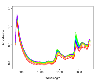
(a) Observed NIR spectra.

(b) Smoothed NIR spectra.

(c) Sample long-run covariance.

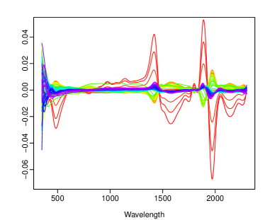
(d) Dynamic FPCA residuals.

Figure 1: NIR absorption spectra of wood panels and residual functions after extraction of the first two dynamic functional components associated with largest empirical eigenvalues of sample long-run covariance function. Using rainbow plots, curves from the distant past are shown in red, and the most recent curves are in violet.

Functional time series methods and theory have witnessed an upsurge in literature contributions in the past two decades (see, e.g., Bosq, 2000; Bosq & Blanke, 2007; Kokoszka & Reimherr, 2013; Aue et al., 2015; Hyndman & Shang, 2009; Klepsch & Klüppelberg, 2017; Klepsch et al., 2017; Li et al., 2020). Most existing functional time series modeling methods, including those in the references cited above, rely on functional principal component analysis (FPCA) to project the intrinsically infinite-dimensional functional objects onto directions of a small number of leading functional principal components. FPCA extracts only the dominant modes of variation of a functional object over its entire domain, with captured information referred to as the “main features” of the considered process. However, the “minor” components neglected by FPCA often have highly localized features possessing information on functional variations over particular short intervals within the function domain. A relatively recent dynamic FPCA introduced by Hörmann et al. (2015) employs long-run covariance to include serial dependence of the data, but suffers the same problem of loss of local features in dimension reduction. The problem of FPCA inadequately extracting local features is illustrated in Figure 1. The eigenanalysis results shown in Figure 1c indicate that the first two leading dynamic functional components explain most functional variation of smoothed NIR spectra (see Section 6 for details of smoothing). Removing the empirical functional principal components from observations, residual functions of dynamic FPCA still contain sharp features around 1300 nm and 1900 nm of wavelength, as shown in Figure 1d. Thus, local features are important for the estimation of functional time series, typically in the study of NIR spectroscopy data that possess multiple significant local features.

Based on molecular overtones and combination vibrations of the investigated molecule, NIR spectroscopy generates complex absorption spectra over a region of the electromagnetic spectroscopy. Since many chemical compounds are known to have characteristic absorption bands over certain spectrum regions between 780–2500 nm, to determine composition materials of an object requires studying particular wavelength ranges (i.e., narrow bands with extreme absorption intensity) of the observed NIR spectrum together instead of examining absorptions one frequency at a time (Burns & Ciurczak, 2007). Thus, a computational method that can extract “local features” covering multiple frequencies of absorption spectrum is important for NIR spectroscopy analysis in practice. Use the wood panel NIR spectrum illustrated in Figure 1 above as an example. The observed local features between 350–2300 nm linked to composition materials, namely, the wood substrate, curing resin, and moisture content (Cao et al., 2018). Subtle changes in experimental conditions such as temperature and pressure lead to variations of absorption bands over a series of trials. Hence, extracting and modeling local features are essential for monitoring the glue curing process of wood panels. Moreover, local features inheriting serial dependence of the original NIR curves can be used to make forecasts for future experiments. In this paper, we aim at developing a methodology for recovering local features that are ignored by FPCA and for using these extracted local features to make more accurate estimations and forecasts for functional time series.

Most existing feature extraction methods attempt to capture local features of functional data by either restricting function domain (see, e.g., Hall & Hooker, 2016; Gellar et al., 2014) or introducing sparseness penalty parameters (see, e.g., Huang et al., 2009; Allen & Weylandt, 2019) during dimension reduction. However, truncating function domains to specific intervals to enhance local feature extraction requires well aligned curves with most local features occurring in the same region. Thus, truncating methods are not suitable for analysis of NIR spectroscopy data that generally focus on identifying non-overlapping absorption spikes in observed spectra. In contrast, sparse FPCA methods impose sparsity penalties in regularized eigendecomposition to identify basis functions with local features. However, a single penalty parameter in practice is not sufficient to accommodate for local features of various magnitudes at different scales. As a result, solving optimization problems to identify the optimal penalty parameter can be tricky: a small penalty results in a significant amount of observation noise falsely identified as local features, while a large penalty fails to preserve peak heights of high-magnitude local features.

Unlike the feature extraction methods mentioned above, Johnstone & Lu (2009) considered extracting principal components of high-dimensional data in wavelet domains. The wavelet bases are considered to be natural for uncovering sparse local features in the signal for the following four reasons. First, wavelet transform is a spatially varying decomposition that adapts its effective “window width” to magnitudes of local oscillations in FPCA residual functions. As a result, wavelet-based algorithms can accurately estimate local features at various scales. Second, orthonormal bases of compactly supported wavelets are particularly good at estimating sharp, highly localized features. This character of wavelet transform allows effective detection of local features associated with chemicals that have very narrow absorption bands (i.e., short intervals of wavelength frequencies) but high intensities (i.e., large absorbance coefficients) in NIR spectroscopy data (Burns & Ciurczak, 2007). Third, the wavelet transform is computationally efficient. For a given orthonormal wavelet basis, feature extraction can be completed in one step of matrix multiplication known as the “discrete wavelet transform” (for further detail on discrete wavelet transform, see Strang (1989); Daubechies (1992)). Fourth and the most important, many types of functional forms encountered in practice, including NIR absorption spectrum, can be sparsely and uniquely represented by a series of wavelet coefficients. Thus, wavelet transform allows a parsimonious representation of local features using only a relatively small number of estimated coefficients.

We propose a two-step algorithm that captures global and local features of functional time series sequentially. Initially, dynamic FPCA is applied to extract global features from the smoothed functional time series. Residuals of dynamic FPCA are then transformed into wavelet domains and block thresholding of wavelet (BTW) coefficients are conducted. Advantages of the FPCA-BTW method over sparse FPCA methods in relation to local feature extraction are demonstrated using simulated data in Section 5.1, and via an empirical application in Section 6. It should be noticed that neither conducting the BTW alone, or conducting the BTW before dynamic FPCA, would effectively capture most global and local features of functional time series in a parsimonious set of estimated wavelet coefficients: First, wavelet approximations requires a fairly large number of coefficients (e.g., $2^{11}$ for the wood panel spectra, and the number of coefficients would increase if more spectrum frequencies are considered) to summarize all global and local features of a continuous function consisting of non-zero signals over its entire domain. More details of wavelet approximations will be presented in Section 2.3 later. Second, implementing BTW leads to a trade-off between preserving the overall smoothness and attaining to fine details of the true signal (see, page 942, Figure 1 in Antoniadis & Fan, 2001, for a depiction of this trade-off). As a result, in practice many local features need to be sacrificed to minimize estimation errors measured by an $L^{2}$ norm for functional time series. In contrast, after conducting FPCA in the initial step of our proposed FPCA-BTW method isolates significant local features in the format of sparse “spikes” over short segments of a function that contains no signal but noise elsewhere. Then, performing the BTW in the second step yields only a small number of non-zero estimated wavelet coefficients containing information on local features as the thresholding algorithm reduces the remaining least important coefficients to zero.

To the best of our knowledge, there is no precedent research focusing on improving FPCA estimation performance via adequately extracting local features contained in “minor” functional components. The principal orthogonal complement thresholding method of Fan et al. (2013) for the estimation of a high dimensional covariance with a conditional sparsity structure is closely analogous to our work as both methods attempt to produce improved estimation performance for processes consisting of finite common global features and sparse local features.

The rest of the paper is organized as follows. In Section 2, we provide necessary background on FPCA and wavelet approximation, before introducing the FPCA-BTW feature extraction method. Implementation details of the proposed method in estimation and forecasting of functional time series are given in Section 3. Section 4 presents asymptotic properties of FPCA-BTW estimators. In Section 5, we use Monte Carlo simulations to illustrate finite sample performances of FPCA-BTW estimators regarding estimation and forecasting of functional time series. Section 6 presents real data applications on NIR spectroscopy data of wood panels. Finally, Section 7 concludes the paper and provides some discussion and directions for future research.

2 Methodology

2.1 Notations

We start by fixing the notations used in this paper. Let $\{\mathcal{X}_{t}(u)\}_{t\in\mathbb{Z}}$ denote random functions defined on a rich enough probability space $(\Omega,\mathcal{A},P)$. Observations $\{\mathcal{X}_{t}(u)\}_{t\in\mathbb{Z}}$ are elements of the Hilbert space $H=L^{2}([0,1])$ equipped with the inner product $\langle x\,,y\rangle=\int_{0}^{1}x(u)y(u)du$. Each $\mathcal{X}_{t}$ is a square integrable function satisfying $\left\lVert\mathcal{X}_{t}\right\rVert^{2}=\int_{0}^{1}\mathcal{X}_{t}^{2}(u)du<\infty$, where the standard norm on $L^{2}([0,1])$ is defined as $\left\lVert x\right\rVert=\langle x,x\rangle^{1/2}$. Define a notation $\mathcal{X}\in L^{p}_{H}(\Omega,\mathcal{A},P)$ such that, for some $p>0$, $E\left\lVert\mathcal{X}\right\rVert^{p}<\infty$.

We consider functional time series $\{\mathcal{X}_{t}(u)\}_{t\in\mathbb{Z}}$ with a general representation given by

$$\mathcal{X}_{t}(u)=\mu(u)+\sum_{k=1}^{K}\beta_{t,k}\phi_{k}(u)+Z_{t}(u)+\varepsilon_{t}(u),\qquad u\in[0,1],$$ (1)

where $\mu(u)=E[\mathcal{X}(u)]$ is the mean function; $\{\phi_{k}(u)\}_{k=1}^{K}$ are real-valued orthogonal functions with $K$ a fixed positive integer; a set of pairwise uncorrelated real numbers $\{\beta_{t,k}\}_{k=1}^{K}=\{\beta_{t,1},\ldots,\beta_{t,K}\}$ satisfy that $var(\beta_{t,i},\beta_{t,j})=0$ for any $i\neq j$; $\{Z_{t}(u)\}_{t\in\mathbb{Z}}$ is a set of functions uncorrelated with $\{\phi_{k}(u)\}_{k=1}^{K}$; $\{\varepsilon_{t}(u)\}_{t\in\mathbb{Z}}$ is $H$-white noise with $E\left\{\varepsilon_{t}(u)\right\}=0$. (See Chapter 3 of Bosq (2000) for further detail about strong white noise function in Hilbert space.) The $\sum_{k=1}^{K}\beta_{t,k}\phi_{k}(u)$ in (1) containing dominant modes of variation of $\{\mathcal{X}_{t}(u)\}_{t\in\mathbb{Z}}$ are referred to as “global features”, whereas $\{Z_{t}(u)\}_{t\in\mathbb{Z}}$ with sparse localized spikes over the function domain $[0,1]$ are referred to as “local features”. We assume that all eigenvalues of long-run covariance of local features are bounded, and the first $K$ eigenvalues of long-run covariance function of global features decrease at the rate of $O(1)$. Extraction of global features and local features from functional time series $\{\mathcal{X}_{t}(u)\}_{t\in\mathbb{Z}}$ are introduced in Sections 2.2 and 2.3, respectively.

2.2 Extraction of global features

A weakly stationary functional time series $\{\mathcal{X}_{t}(u)\}_{t\in\mathbb{Z}}$ satisfies that, for all $t\in\mathbb{Z}$, (a) $\mathcal{X}_{t}(u)\in L^{2}([0,1])$, (b) $E[\mathcal{X}_{t}(u)]=E[\mathcal{X}_{0}(u)]=\mu(u)$, and (c) for all $\ell\in\mathbb{Z}$ and $u,s\in[0,1]$, $$c_{\ell}(u,s)=\text{cov}[\mathcal{X}_{0}(u),\mathcal{X}_{\ell}(s)]=\text{cov}[\mathcal{X}_{t+\ell}(u),\mathcal{X}_{t}(s)],$$ (2) with $\text{cov}[\mathcal{X}(u),\mathcal{X}(s)]=E[\{\mathcal{X}(u)-\mu(u)\}\{\mathcal{X}(s)-\mu(s)\}]$. $C_{\ell}$ induces an operator $L^{2}([0,1])\rightarrow L^{2}([0,1])$ given by

$$C_{\ell}(x)(u)=\int_{0}^{1}C_{\ell}(u,s)x(s)\mathop{}\!\mathrm{d}s,\qquad x\in L^{2}([0,1]),\quad u,s\in[0,1].$$

When $\ell=0$, the autocovariance operator $C_{\ell}$ has a special case of covariance operator $C_{0}$ defined by $C_{0}(x)=\int_{0}^{1}C_{0}(u,s)x(s)\mathop{}\!\mathrm{d}s$ for $x\in L^{2}([0,1])$ and $u,s\in[0,1]$.

In practice, $\{\mathcal{X}_{t}(u)\}_{t\in\mathbb{Z}}$ often consists of serially correlated observed trajectories. To incorporate serial dependence carried by lagged observations, recent studies (see, e.g., Rice & Shang, 2017; Shang, 2019) suggest computing a long-run covariance function $C(u,s)$ as

$$C(u,s)=\sum_{\ell=-\infty}^{\infty}c_{\ell}(u,s),\qquad u,s\in[0,1].$$ (3)

A long-run covariance operator $C$ is then defined as

$$C(x)(u)=\int_{0}^{1}C(u,s)x(s)\mathop{}\!\mathrm{d}s\qquad x\in L^{2}([0,1]),\quad u,s\in[0,1].$$

The symmetric positive-definite Hilbert-Schmidt operator $C$ admits a decomposition as

$$C(x)=\sum_{k=1}^{\infty}\lambda_{k}\langle\phi_{k}\,,x\rangle\phi_{k},\qquad x\in L^{2}([0,1]),$$

where $\{\lambda_{k}\}_{k\in\mathbb{Z}^{+}}$ are the nonincreasing eigenvalues, and $\{\phi_{k}\}_{k\in\mathbb{Z}^{+}}$ the corresponding orthonormal eigenfunctions such that $C(\phi_{k})=\lambda_{k}\phi_{k}$, and $\langle\phi_{i}\,,\phi_{j}\rangle=1$ iff $i=j$. The Karhunen–Loève expansion of a stochastic process $\mathcal{X}_{t}(u)$ is then given by

$$\mathcal{X}_{t}(u)=\mu(u)+\sum_{k=1}^{\infty}{\beta}_{t,k}\phi_{k}(u),$$

where the $k$th functional component score $\beta_{t,k}$ is a projection of $\overline{\mathcal{X}}_{t}(u)=\mathcal{X}_{t}(u)-\mu(u)$ in the direction of the $k$th eigenfunction $\phi_{k}(u)$, that is, $\beta_{k}=\langle\overline{\mathcal{X}}_{t}\,,\phi_{k}\rangle$.

According to (1), the main features of the infinite-dimensional $\{\mathcal{X}_{t}(u)\}_{t\in\mathbb{Z}}$ can be summarized by its first $K$ leading components as

$$\mathcal{X}_{t}(u)=\mu(u)+\sum_{k=1}^{K}{\beta}_{t,k}\phi_{k}(u)+e_{t}(u),$$ (4)

where $\{e_{t}(u)\}_{t\in\mathbb{Z}}$ are error functions after truncation. According to Theorem 2 of Hörmann et al. (2015), the linear combination of $\sum_{k=1}^{K}{\beta}_{t,k}\phi_{k}(u)$ obtained by dynamic FPCA satisfies that, for any other orthonormal basis $\{\varphi_{k}\}_{k\in\mathbb{Z}^{+}}$ of Hilbert space $H$,

$$E\left[\left\lVert\overline{\mathcal{X}}_{t}-\sum_{k=1}^{K}\beta_{t,k}\phi_{k}\right\rVert^{2}\right]\leq E\left[\left\lVert\overline{\mathcal{X}}_{t}-\sum_{k=1}^{K}\langle\mathcal{X}_{t}\,,\varphi_{k}\rangle\varphi_{k}\right\rVert^{2}\right].$$ (5)

In rare cases, functional time series $\{\mathcal{X}_{t}(u)\}_{t\in\mathbb{Z}}$ may possess weak serial dependence. The significance of serial dependence can be determined according to the hypothesis test of Horváth et al. (2016). Functional observations are treated as independent if $c_{\ell}$ of (2) at all lags apart from $\ell=0$ are tested to be negligible. A process that decomposes the covariance operator $C_{0}$ to extract global features is often referred to as static FPCA to distinguish it from dynamic FPCA. In the remaining of this paper, we present feature extraction results obtained by dynamic FPCA and include feature extraction results associated with static FPCA in the Supplementary document. The aim of this paper is to demonstrate the proposed local feature extraction method can be applied to improve performances of static FPCA and dynamic FPCA, instead of comparing performances of the two versions of FPCA.

It can be seen from (5) that dynamic FPCA can find an optimal representation of global features of $\{\mathcal{X}_{t}(u)\}_{t\in\mathbb{Z}}$, but ignores most local features $\{Z_{t}(u)\}_{t\in\mathbb{Z}}$. Our proposed two-step feature extraction method will continue to capture any remaining local features from FPCA residuals, as described in Section 2.3.

2.3 Extraction of local features

To extract sharp and highly localized features from FPCA residuals, we consider an orthonormal system of wavelet functions. Wavelet functions combine compact support with various degrees of smoothness, which enables the extraction of signals at a variety of different scales. It has been tested that wavelets can effectively isolate signals from noisy functions in statistical applications (see, e.g., Antoniadis, 2007; Ogden, 1997). Most recent wavelet applications in statistics adopt the approach of Daubechies (1992) to define two related and specially selected orthonormal parent wavelet functions: the scaling function $\psi$ and the mother wavelet $\Psi$. Wavelets can then be generated by dilation and translation as

$$\psi_{j,p}=2^{j/2}\psi(2^{j}t-p),\quad\Psi_{j,p}=2^{j/2}\Psi(2^{j}t-p),\qquad(j\in\mathbb{Z}^{+},\quad p=1,\ldots,2^{j}),$$

where the index $j$ represents resolution level in wavelet decomposition. This wavelet system produces wavelet functions forming an orthonormal wavelet basis in $L^{2}([0,1])$. With a primary decomposition level $j_{0}\geq 0$, local features $\{Z_{t}(u)\}_{t\in\mathbb{Z}}$ admit a decomposition given by

$$Z_{t}(u)=\sum_{p=1}^{2^{j_{0}}}D^{\prime}_{j_{0},p,t}\psi_{j_{0},p}(u)+\sum_{j={j_{0}}}^{\infty}\sum_{p=1}^{2^{j}}D_{j,p,t}\Psi_{j,p}(u),$$ (6)

where wavelet coefficients are defined as

$$D^{\prime}_{j_{0},p,t}=\int_{0}^{1}Z_{t}(u)\psi_{j_{0},p}(u)\mathop{}\!\mathrm{d}u,\quad D_{j,p,t}=\int_{0}^{1}Z_{t}(u)\Psi_{j,p}(u)\mathop{}\!\mathrm{d}u.$$

“Approximations” and “details” of $Z_{t}(u)$ are stored in wavelet coefficients $D^{\prime}_{j_{0},p,t}$ and $D_{j,p,t}$, respectively (Mallat, 2009).

According to (1), residual functions $\{e_{t}(u)\}_{t\in\mathbb{Z}}$ consist of highly localized features $Z_{t}(u)$ and random noise $\varepsilon_{t}(u)$ given by

$$e_{t}(u)=Z_{t}(u)+\varepsilon_{t}(u).$$

The wavelet transform of $e_{t}(u)$ can be expressed as

$$e_{t}(u)=\sum_{p=1}^{2^{j_{0}}}\widetilde{D}^{\prime}_{j_{0},p,t}\psi_{j_{0},p}(u)+\sum_{j={j_{0}}}^{\infty}\sum_{p=1}^{2^{j}}\widetilde{D}_{j,p,t}\Psi_{j,p}(u),$$

where the empirical wavelet coefficients $\widetilde{D}^{\prime}_{j_{0},p,t}$ and $\widetilde{D}_{j,p,t}$ are given by

$$\widetilde{D}^{\prime}_{j_{0},p,t}=\int_{0}^{1}e_{t}(u)\psi_{j_{0},p}(u)\mathop{}\!\mathrm{d}u,\quad\widetilde{D}_{j,p,t}=\int_{0}^{1}e_{t}(u)\Psi_{j,p}(u)\mathop{}\!\mathrm{d}u.$$

Wavelet coefficients related to detailed structure of $e_{t}(u)$ and $Z_{t}(u)$ thus satisfy that, for any $t\in\mathbb{Z}$,

$$\widetilde{D}_{j,p,t}=D_{j,p,t}+\epsilon_{j,p,t},\qquad(j\in\mathbb{Z}^{+},\quad p=1,\ldots,2^{j}),$$ (7)

where $\epsilon_{j,p,t}=\int_{0}^{1}\varepsilon_{t}(u)\Psi_{j,p}(u)\mathop{}\!\mathrm{d}u$ represents a wavelet transform of contamination noise. Since local features $\{Z_{t}(u)\}_{t\in\mathbb{Z}}$ are sparse, a vector of wavelet coefficients $D_{t}=\{D_{j_{0},1,t},\ldots,\allowbreak D_{j_{0},2^{j_{0}},t},\ldots\}$ contains many zeros. Extracting local features is then equivalent to determining non-zero wavelet coefficients $D_{j,p,t}$. From a statistical modeling perspective, the denoising problem of (7) has been commonly approached by shrinking the empirical wavelet coefficients $\{\widetilde{D}_{j,p,t}\}_{j\in\mathbb{Z}^{+},p=1,\ldots,2^{j}}$ one by one (see, e.g., Donoho & Johnstone, 1994; Antoniadis & Fan, 2001). However, local features of functional data often occur over short intervals within the function domain that correspond to several consecutive wavelet coefficients at fine resolution levels. To determine chemical content of an object by NIR spectroscopy, simultaneously considering the non-zero wavelet coefficients corresponding to certain distinctive absorption bands of known chemical compounds provides more accurate composition results than examining absorption value at any single frequency. For example, local features depicting extreme absorption bands of approximately 1900 nm, shown in Figure 1d, are summarized into 21 consecutive empirical wavelet coefficients at the resolution level $j=11$. Thus, to enhance extraction of local features, adjacent wavelet coefficients should be modeled together as a group. For this purpose, we adopt a block thresholding approach of Cai (2002) to make simultaneous selection of empirical wavelet coefficients in groups as follows. At each resolution level $j$, divide the empirical wavelet coefficients $\widetilde{D}_{j,p,t}$ into non-overlapping blocks of length $L$. Denote indices of the coefficients in the $a$th block at level $j$ by $j_{a}$, i.e., $j_{a}=\{(j,p):(a-1)L+1\leq p\leq aL\}$. Let $S^{2}_{j_{a}}=\sum_{p\in j_{a}}\widetilde{D}_{j,p,t}^{2}$ denote the sum of squares of the empirical coefficients in the block. A block is significant if its $S^{2}_{j_{a}}$ is larger than a threshold $T_{w}=\lambda^{\star}L\sigma^{2}/2^{J}$, where $\lambda^{\star}$ is a threshold constant and $\sigma$ is the noise level. Retaining significant wavelet coefficients while discarding the remaining negligible coefficients leads to a local feature estimator as

$$\widehat{Z}_{t}(u)=\sum_{k=0}^{2^{j_{0}}}\widetilde{D}^{\prime}_{j_{0},p,t}\psi_{j_{0},p}(u)+\sum_{j={j_{0}}}^{J-1}\sum_{a}\left(\sum_{p\in j_{a}}\widetilde{D}_{j,p,t}\Psi_{j,p}(u)\mathds{1}(S^{2}_{j_{a}}>T_{w})\right),$$ (8)

where $a$ varies for different resolution levels and $\mathds{1}(\cdot)$ represents the binary indicator function.

In (8), the block length $L$ and the threshold constant $T_{w}$ together control global and local adaptivity of the estimator $\widehat{Z}_{t}(u)$. A global adaptive estimator adjusts to the overall regularity of the target function, and a locally adaptive estimator focuses on optimally adapting to subtle and highly localized features along the curve. The optimal selection of parameters $L$ and $T_{w}$, together with other implementation details about the FPCA-BTW feature extraction method, are described in Section 3.

3 Implementation details

3.1 Long-run covariance estimation

We first present technical details of extracting global features of a finite sample functional time series. To consider serial dependence of stationary functional observations $\{\mathcal{X}_{t}(u)\}_{t=1}^{T}$, we compute the empirical long-run covariance function as

$$\widehat{C}_{h,q}(u,s)=\sum_{\ell=-T}^{T}W_{q}\left(\frac{\ell}{h}\right)\widehat{c}_{\ell}(u,s),$$ (9)

where $W_{q}$ is a symmetric weight function with bounded support of order $q$, and $h$ is a bandwidth parameter; the estimator of $c_{\ell}(u,s)$ is defined in the form of

$$\widehat{c}_{\ell}(u,s)=\begin{cases}\frac{1}{T}\sum_{j=1}^{T-\ell}\left[\mathcal{X}_{j}(u)-\widehat{\mu}(u)\right]\left[\mathcal{X}_{j+\ell}(s)-\widehat{\mu}(s)\right],&\ell\geq 0;\\ \frac{1}{T}\sum_{j=1-\ell}^{T}\left[\mathcal{X}_{j}(u)-\widehat{\mu}(u)\right]\left[\mathcal{X}_{j+\ell}(s)-\widehat{\mu}(s)\right],&\ell<0.\end{cases}$$

The optimal bandwidth parameter $h$ is selected via the “plug-in” algorithm proposed in Rice & Shang (2017). More details about estimating the corresponding $\widehat{C}_{\widehat{h}_{\text{opt}}}(u,s)$ are provided in Appendix LABEL:app_b1 in the Supplementary document. The empirical long-run covariance operator is then given by

$$\widehat{C}(x)(u)=\int_{0}^{1}\widehat{C}_{\widehat{h}_{\text{opt}}}(u,s)x(s)\mathop{}\!\mathrm{d}s,\qquad x\in L^{2}([0,1]).$$

Performing eigendecomposition on the empirical long-run covariance operator yields

$$\widehat{C}(x)=\sum_{k=1}^{\infty}\widehat{\lambda}_{k}\langle\widehat{\phi}_{k}\,,x\rangle\widehat{\phi}_{k},\qquad x\in L^{2}([0,1]),$$

where $\{\widehat{\phi}_{k}\}_{k\in\mathbb{Z^{+}}}$ are the empirical eigenfunctions, and $\{\widehat{\lambda}_{k}\}_{k\in\mathbb{Z^{+}}}$ are associated eigenvalues. To facilitate dimension reduction, the dimension of global features $\widehat{K}$ need to be empirically determined. Existing functional time series methods generally select $\widehat{K}$ by requiring that retained functional components should explain a certain level of the total variance, approximately 85% (see, e.g., Chiou, 2012; Hörmann et al., 2015; Shang, 2019). However, this criterion of cumulative percentage of explained variation has the disadvantage of incorrectly selecting too many components as global features when fast-diverging eigenvalues are present in FPCA analysis. To precisely extract global features, following Li et al. (2020), the value of $K$ is determined as the integer minimizing ratios of two adjacent empirical eigenvalues given by

$$\widehat{K}=\operatorname*{\arg\!\min}_{1\leq k\leq k_{max}}\left\{\frac{\widehat{\lambda}_{k+1}}{\widehat{\lambda}_{k}}\times\mathds{1}\left(\frac{\widehat{\lambda}_{k}}{\widehat{\lambda}_{1}}\geq\tau\right)+\mathds{1}\left(\frac{\widehat{\lambda}_{k}}{\widehat{\lambda}_{1}}<\tau\right)\right\},$$ (10)

where $k_{max}$ is a prespecified positive integer, $\tau$ is a prespecified small positive number, and $\mathds{1}(\cdot)$ is the indicator function. When without priori information about a possible maximum of $K$, it is unproblematic to choose a relatively large $k_{max}$, e.g., $k_{max}=\#\{k|\widehat{\lambda}_{k}\geq\sum_{k=1}^{T}\widehat{\lambda}_{k}/T,k\geq 1\}$ (Ahn & Horenstein, 2013). Given that the small empirical eigenvalues $\widehat{\lambda}_{k}$ for some $K<k<k_{max}$ are likely to be practically zero, we adopt the threshold constant $\tau=1/\ln({\max{\{\widehat{\lambda}_{1}},T\}})$ to ensure consistency of $\widehat{K}$.

As described in Section 2.2, it is possible to have nearly independent $\{\mathcal{X}_{t}(u)\}_{t=1}^{T}$ in practice. The sample covariance operator of independent observations is computed as

$$\widehat{C}_{0}(x)(u)=\int_{0}^{1}\widehat{c}_{0}(u,s)x(s)\mathop{}\!\mathrm{d}s,\qquad x\in L^{2}([0,1]),$$

where $\widehat{c}_{0}(u,s)=\frac{1}{T}\sum_{t=1}^{T}[\mathcal{X}_{t}(u)-\widehat{\mu}(u)][\mathcal{X}_{t}(s)-\widehat{\mu}(s)]$ is the empirical covariance kernel with the empirical mean function $\widehat{\mu}(u)=\frac{1}{T}\sum_{t=1}^{T}\mathcal{X}_{t}(u)$. For such data static FPCA is applied to extract global features from $\widehat{C}_{0}(x)(u)$ using the same criterion as (10).

With FPCA results, functional time series can be estimated by

$$\widehat{\mathcal{X}}_{t}(u)=\widehat{\mu}(u)+\sum_{k=1}^{\widehat{K}}\widehat{\beta}_{t,k}\widehat{\phi}_{k}(u),$$

where $\sum_{k=1}^{K}\widehat{\beta}_{t,k}\widehat{\phi}_{k}(u)$ represents the extracted global features, with the empirical principal component scores defined by $\widehat{\beta}_{t,k}=\int_{0}^{1}\left[\mathcal{X}_{t}(u)-\widehat{\mu}(u)\right]\widehat{\phi}_{k}(u)\mathop{}\!\mathrm{d}u$. Removing the estimated mean function and the extracted global features from functional observations leaves residual functions given by

$$\widehat{e}_{t}(u)=\mathcal{X}_{t}(u)-\widehat{\mu}(u)-\sum_{k=1}^{\widehat{K}}\widehat{\beta}_{t,k}\widehat{\phi}_{k}(u).$$

In Section 3.2, we present details of recovering local features from $\{\widehat{e}_{t}(u)\}_{t=1}^{T}$ through block thresholding of wavelet coefficients.

3.2 Estimation of wavelet coefficients

The continuous wavelet transform formalized by Grossmann & Morlet (1984) can be implemented in computer software such as R (R Core Team, 2020) to extract local features from FPCA residuals $\{\widehat{e}_{t}(u)\}_{t=1}^{T}$. However, in practice, we most likely only observe discretized values $\{\mathcal{X}_{t}(u_{i})\}_{i=1}^{n_{t}}$, with $n_{t}$ denoting the number of grid points in the $t$-th curve. Removing global features evaluated at each grid point leaves discrete residuals $\{\widehat{e}_{t}(u_{i})\}_{i=1}^{n_{t}}$. When equally spaced grids satisfy $n_{t}=2^{J}$ for $t=1,\ldots,T$, wavelet transform of $\{\widehat{e}_{t}(u)\}_{t=1}^{T}$ can be performed in $O(2^{J})$ operations (Mallat, 1989).

In situations when functional observations have nondyadic, varying or unequally spaced grid points, the non-linear regularized Sobolev interpolator of Antoniadis & Fan (2001) is adopted to perform the wavelet transform. Local feature extraction can then be completed in the following steps. First, select an orthonormal wavelet family to obtain an orthogonal DWT base matrix ${W}$ with dimension $N\times N$, where $N=2^{J}\geq\max(n_{1},\ldots,n_{T})$ is a dyadic integer. There are many discrete wavelet families available in the literature. We follow Zhao et al. (2012) and consider the Daubechies least asymmetric wavelets with 10 vanishing moments in the analysis of NIR spectroscopy data. Denote ${A}$ as a matrix of dimension $n_{t}\times N$ whose $i$th row corresponds to the row of the matrix ${W}^{{\mathrm{\scriptscriptstyle T}}}$. We interpolate the vector $\widehat{{e}}_{t}=[\widehat{e}_{t}(u_{1}),\ldots,\widehat{e}_{t}(u_{n_{t}})]^{{\mathrm{\scriptscriptstyle T}}}$ as

$$\widetilde{{D}}_{t}={A}^{{\mathrm{\scriptscriptstyle T}}}\widehat{{e}}_{t},$$ (11)

where $\widetilde{{D}}_{t}=[\widetilde{D}^{\prime}_{j_{0},1,t},\ldots,\widetilde{D}^{\prime}_{j_{0},2^{j_{0}},t},\widetilde{D}_{j_{0},1,t},\ldots,\widetilde{D}_{j_{0},2^{j_{0}},t},\ldots,\widetilde{D}_{J-1,1,t},\ldots,\widetilde{D}_{J-1,2^{J-1},t}]^{{\mathrm{\scriptscriptstyle T}}}$ is a vector of size $N$ (Antoniadis & Fan, 2001). The optimal parameters for block thresholding are then selected according to Cai (2002). Specifically, for the block size $L$ and the threshold constant $\lambda^{\star}$ in (8), $L=2^{\lfloor\log_{2}(\ln(2^{J}))\rfloor}$ and $\lambda^{\star}=4.5052$ are chosen. Noise level of residual functions are estimated by taking the median absolute deviation (MAD) as

$$\widehat{\sigma}=\frac{\text{MAD}\{\widetilde{D}_{J-1,p,t}/v_{J-1,p,t}^{1/2}:v_{J-1,p,t}>0.0001\}}{0.6745},$$

where $\{\widetilde{D}_{J-1,p,t}\}_{p=1,\ldots,2^{J-1}}$ are the empirical wavelet coefficients at the resolution level $J-1$, and $\{v_{J-1,p,t}\}_{p=1,\ldots,2^{J-1}}$ are diagonal elements of the matrix ${V}={A}^{{\mathrm{\scriptscriptstyle T}}}{A}$ (Antoniadis & Fan, 2001). Next, the first-round block thresholding is implemented according to (8), and intermediate results are denoted as $\widetilde{{D}}^{\ast}_{t}$. Subtracting the inverse transform of $\widetilde{{D}}^{\ast}_{t}$ from discrete residuals gives

$$\widehat{{e}}^{\ast}_{t}=\widehat{{e}}_{t}-{A}\widetilde{{D}}^{\ast}_{t}.$$

The second round empirical wavelet coefficients are then computed as

$$\widetilde{{D}}^{\dagger}_{t}=\widetilde{{D}}^{\ast}_{t}+{A}^{{\mathrm{\scriptscriptstyle T}}}\widehat{{e}}^{\ast}_{t}.$$

Finally, performing block thresholding again on $\widetilde{{D}}^{\dagger}_{t}$ yields the final BTW coefficients $\widehat{{D}}_{t}=[\widehat{D}^{\prime}_{j_{0},1,t},\ldots,\widehat{D}^{\prime}_{j_{0},2^{j_{0}},t},\widehat{D}_{j_{0},1,t},\ldots,\widehat{D}_{j_{0},2^{j_{0}},t},\ldots,\widehat{D}_{J-1,1,t},\ldots,\widehat{D}_{J-1,2^{J-1},t}]^{{\mathrm{\scriptscriptstyle T}}}$ with many zero entries reflecting the sparseness of the local features. Note that we keep the “approximation” wavelet coefficients unchanged as $\widehat{D}^{\prime}_{j_{0},p,t}=\widetilde{D}^{\prime}_{j_{0},p,t}$ for all $p=1,\ldots,2^{j_{0}}$. According to Solo (2001), implementing the estimation method of Antoniadis & Fan (2001) through a two-round block thresholding process simplifies computation. Applying the above procedure to each discrete residual function $\widehat{e}_{t}$ leads to a sparse $N\times T$ matrix of BTW coefficients $\widehat{{D}}=[\widehat{{D}}_{1},\ldots,\widehat{{D}}_{T}]$. The extracted local features are then given by a product ${A}\widehat{{D}}$.

Using the extracted global and local features, we can make improved estimation of the considered functional process and its covariance structure, and produce more accurate forecasts. We demonstrate applications of the proposed feature extraction method using simulated samples in Section 5 and real NIR spectroscopy data in Section 6. Additional technical details about long-run covariance estimation and applications of the FPCA-BTW method are provided in Appendix LABEL:app_b2 in the supplementary document.

4 Asymptotic properties

Before presenting assumptions and asymptotic results of long-run covariance based FPCA-BTW estimators, we introduce some notations. Let $\mathcal{L}=\mathcal{L}(H,H)$ be the space of bounded linear operators from $H$ to $H$. We define the operator norm $\left\lVert A\right\rVert_{\mathcal{L}}=\sup_{\left\lVert x\right\rVert\leq 1}\left\lVert A(x)\right\rVert$ for $A\in\mathcal{L}$. The operator $A$ is compact if there exists two orthonormal bases $\{\nu_{k}\}$ and $\{v_{k}\}$, and a real sequence $\{\lambda_{k}\}$ converging to zero, such that

$$A(x)=\sum_{k=1}^{\infty}\lambda_{k}\langle x\,,\nu_{k}\rangle v_{k},\qquad x\in H.$$

A compact operator is said to be a Hilbert-Schmidt operator if $\sum_{k=1}^{\infty}\lambda_{k}^{2}<\infty$. We denote the Hilbert-Schmidt norm by $\left\lVert A\right\rVert_{\mathcal{S}}$. For any Hilbert-Schmidt operator $A$, one can show that $\left\lVert A\right\rVert_{\mathcal{S}}^{2}=\sum_{k\geq 1}\lambda_{k}^{2}$ and $\left\lVert A\right\rVert_{\mathcal{L}}\leq\left\lVert A\right\rVert_{\mathcal{S}}$ (Horváth & Kokoszka, 2012, Chapter 2).

Assumption 1.

Functions $\{\mathcal{X}_{t}(u),u\in[0,1]\}_{t\in\mathbb{Z}}$ are $L^{4}\operatorname{-}m\operatorname{-}$approximable, taking values in $L^{2}([0,1])$, satisfying the following conditions:

1. $X_{t}$ admits the representation $\mathcal{X}_{t}=f(\delta_{t},\delta_{t-1},\delta_{t-2}\ldots,\delta_{t-m+1},\delta_{t-m},\delta_{t-m-1},\ldots)$ with $\delta_{i}$ i.i.d. elements taking values in a measurable space $S$ and a measurable function $f:\mathcal{S}^{\infty}\rightarrow H$.

2. $E\left\lVert\mathcal{X}_{0}\right\rVert^{4+d}<\infty$ for some $d>0$, and

3. $\{\mathcal{X}_{t}(u),u\in[0,1]\}_{t\in\mathbb{Z}}$ can be approximated by $m$-dependent sequences

   $$\mathcal{X}_{t}^{(m)}=f(\delta_{t},\delta_{t-1},\delta_{t-2},\ldots,\delta_{t-m+1},\delta_{t,t-m}^{(m)},\delta_{t,t-m-1}^{(m)},\ldots),$$

   where $\{\delta_{t,i}^{(m)}\}$ are independent copies of sequence $\{\delta_{t}\}_{-\infty<t<\infty}$ defined on the same measurable space $S$ such that $\sum_{m=1}^{\infty}\upsilon_{4}(\mathcal{X}_{t}-\mathcal{X}_{t}^{(m)})<\infty$ with $\upsilon_{4}(\mathcal{X}_{t}-\mathcal{X}_{t}^{(m)})=\left\{E\left\lVert\mathcal{X}_{t}-\mathcal{X}_{t}^{(m)}\right\rVert^{4}\right\}^{1/4}$.

Remark 1.

Assumption 1 follows the dependence concept for functional time series introduced in Hörmann & Kokoszka (2010). This assumption is often considered as equivalent conditions to the classic mixing conditions in function spaces (see, e.g., Berkes et al., 2016; Horváth et al., 2016; Rice & Shang, 2017). Condition (iii) specifies the level of dependence that is allowed within process $\{\mathcal{X}_{t}(u)\}_{t\in\mathbb{Z}}$ in relation to how well it can be approximated by finite $m$-dependent processes. Condition (iii) can also be satisfied when $\upsilon_{4}(\mathcal{X}_{t}-\mathcal{X}_{t}^{(m)})=O(m^{-\rho})$ for some $\rho>4$. Roughly speaking, the $\mathcal{X}_{t}^{(m)}$ defined by the coupling construction in Condition (iii) can be determined by the first $m$ elements $\delta_{t},\delta_{t-1},\ldots,\delta_{t-m+1}$. When the measurable space $S$ coincides with $H$, the sequence $\{\widetilde{\mathcal{X}}_{t}^{(m)}\}$ given by

$$\widetilde{\mathcal{X}}_{t}^{(m)}=f(\delta_{t},\delta_{t-1},\delta_{t-2},\ldots,\delta_{t-m+1},0,0,\ldots)$$

is also strictly stationary and $m$-dependent, satisfying $\sum_{m=1}^{\infty}\upsilon_{4}(\mathcal{X}_{t}-\widetilde{\mathcal{X}}_{t}^{(m)})<\infty$.

Assumption 2.

The kernel function $W_{q}(\cdot)$ in (9) satisfies the following standard conditions:

$$W_{q}(0)=1,\quad W_{q}(u)\leq 1,\quad W_{q}(u)=W_{q}(-u),\quad W_{q}(u)=0\text{ if }\left|u\right|>g\text{ for some constant }g>0,$$

$$\text{and }W_{q}(u)\text{ is Lipschitz continuous on }[-g,g].$$ (12)

There exists a $q>0$ such that

$$0<\lim_{u\to 0}\frac{W_{q}(u)-1}{\left|u\right|^{q}}=\mathcal{W}_{q}<\infty,$$

and there exists $q^{\prime}>q$ such that

$$\sum_{\ell=-\infty}^{\infty}\left|\ell\right|^{q^{\prime}}\left\lVert c_{\ell}\right\rVert<\infty,$$

where $c_{\ell}$ is the lag-$\ell$ autocovariance function defined in (2).

Remark 2.

Assumption 2 limits the growing rate of $W_{q}(u)$ at $u=0$, with $q$ referred to as the characteristic exponent of the kernel function by Parzen (1957). The smoother the kernel $W_{q}(u)$ at zero, the larger the value of $q$ for which $\mathcal{W}_{q}$ is finite. This assumption has been widely adopted in studies on limit behaviors of the long-run covariance estimator (e.g., Berkes et al., 2016; Rice & Shang, 2017).

The conditions in Assumptions 1 and 2 can be easily verified for most stationary time series models based on independent innovations. In the following example we illustrate the applicability of Assumptions 1 and 2 using a standard functional linear process (Bosq, 2000).

Example 1.

(Functional autoregressive process). Suppose $\Phi\in\mathcal{L}$ satisfies $\left\lVert\Phi\right\rVert_{\mathcal{L}}<1$. Let $\{\varepsilon_{t}\}_{t\in\mathbb{Z}}$ be a sequence of i.i.d. random elements of mean zero taking values in $L^{2}([0,1])$ satisfying $E\left\lVert\varepsilon_{0}\right\rVert^{2}<\infty$. There exists a unique stationary sequence of random process $\{\mathcal{X}_{t}(u),u\in[0,1]\}_{t\in\mathbb{Z}}$ taking the form

$$\mathcal{X}_{t}(u)=\Phi(\mathcal{X}_{t-1})(u)+\varepsilon_{t}(u),$$

which is referred to as functional autoregressive process of order one (FAR(1)). The FAR(1) process admits the expansion $\mathcal{X}_{t}(u)=\sum_{j=0}^{\infty}\Phi^{j}(\varepsilon_{t-j})(u)$ where $\Phi^{j}$ is the $j$th iterate of the operator $\Phi$. According to Condition (iii), we can define an approximation $\mathcal{X}_{t}^{(m)}(u)=\sum_{j=0}^{m-1}\Phi^{j}(\varepsilon_{t-j})(u)+\sum_{j=m}^{\infty}\Phi^{j}(\varepsilon_{t-j}^{(m)})(u)$. The approximation error can then be expressed as $\mathcal{X}_{t}(u)-\mathcal{X}_{t}^{(m)}(u)=\sum_{j=m}^{\infty}(\Phi^{j}(\varepsilon_{t-j})(u)-\Phi^{j}(\varepsilon_{t-j}^{(m)})(u))$. Using Cauchy–Schwarz inequality, it can be verified that every operator $A\in\mathcal{L}$ satisfies $\upsilon_{4}(A(\mathcal{X}))\leq\left\lVert A\right\rVert_{\mathcal{L}}\upsilon_{4}(\mathcal{X})$. Then, it follows that $\upsilon_{4}(\mathcal{X}_{t}-\mathcal{X}_{t}^{(m)})\leq 2\sum_{j=m}^{\infty}\left\lVert\Phi\right\rVert^{j}_{\mathcal{L}}\upsilon_{4}(\mathcal{X}_{t}-\mathcal{X}_{t}^{(m)})=O(\left\lVert\Phi\right\rVert^{m}_{\mathcal{L}}\upsilon_{4}(\varepsilon_{0}))$. This shows that for the FAR(1) process, Assumption 1 holds as long as $\left\lVert\varepsilon_{0}\right\rVert$ has moments up to order $4+d$ for some $d>0$. In addition, Lemma 3.2 of Bosq (2000) indicates that $E\left\lVert c_{\ell}\right\rVert^{2}\leq\left\lVert\Phi\right\rVert^{\ell}_{\mathcal{L}}E\left\lVert\mathcal{X}_{0}\right\rVert^{2}$. Assumption 2 then holds since we have assumed that $E\left\lVert\mathcal{X}_{0}\right\rVert^{2}\leq\sum_{j=0}^{\infty}\left\lVert\Phi\right\rVert^{j}_{\mathcal{L}}E\left\lVert\varepsilon_{0}\right\rVert^{2}<\infty$.

To ensure the consistency of the long-run covariance estimator $\widehat{C}_{h,q}$ in (9), we impose the following condition on the bandwidth parameter $h$.

Assumption 3.

The bandwidth parameter $h$ of long-run covariance estimator in (9) satisfies

$$h=h(T)\to\infty\textnormal{ and }\frac{h(T)}{T}\to 0,\textnormal{ as }T\to\infty.$$

We use the optimal value of $h$ selected according to the plug-in bandwidth selection procedure of Rice & Shang (2017) in developing asymptotic results and conducting simulation and empirical studies in this paper.

Remark 3.

Assumption 3 is a weaker and more standard condition compared to the one used in the Theorem 4.2 of Hörmann & Kokoszka (2010), that is, $h^{2}/T\rightarrow 0$. Details of the plug-in algorithm are provided in Appendix LABEL:app_b1 in the supplementary document.

Assumption 4.

The eigenvalues of the long-run covariance operator $C$ are finite, positive, and distinctive, i.e., $\infty>\lambda_{1}>\lambda_{2}>\ldots$. There exists a positive integer $K$ such that

$$\frac{\sum_{k=K+1}^{\infty}\lambda_{k}}{\sum_{k=1}^{K}\lambda_{k}}=o(1).$$ (13)

Remark 4.

Distinctive eigenvalues of covariance operators are commonly adopted in the literature to ensure identification of eigenfunctions (see, e.g., Hörmann & Kokoszka, 2010; Hörmann et al., 2015). Assumption 13 requires that the sum of the “insignificant” eigenvalues $\{\lambda_{K+1},\lambda_{K+2}\ldots\}$ tend to zero sufficiently rapidly. Thus, the $K$-dimensional global feature contains “most information” of $\mathcal{X}_{t}(u)$ (see e.g., Hall & Vial, 2006; Bathia et al., 2010). Roughly speaking, Assumption 13 requires that the first $K$ eigenvalues $\{\lambda_{1},\ldots\lambda_{K}\}$ have greater orders than the remaining eigenvalues in the sense of (13). For example, denoting $a/b\rightarrow 1$ by “$a\sim b$”, Li et al. (2020) proposed that eigenvalues of long-run covariance function satisfying the conditions (a) $\lambda_{k}\sim\rho_{k}T^{3-2\alpha_{k}}$for $k=1,\ldots,K$ with coefficients $\infty>\rho_{1}\geq\rho_{2}\geq\ldots\rho_{K}>0$ and $1/2<\alpha_{1}<\alpha_{2}<\ldots<\alpha_{K}<1$, and (b) $\sum_{k=K+1}^{\infty}\lambda_{k}=O(T)$. Given that $T^{3-2\alpha_{1}}>T^{3-2\alpha_{2}}>\ldots T^{3-2\alpha_{K}}>T$ for a fixed $K$, the sum of $\sum_{k=1}^{K}\lambda_{k}$ has an order of $T^{3-2\alpha_{1}}$. It can then be readily seen that $\sum_{k=K+1}^{\infty}\lambda_{k}/\sum_{k=1}^{K}\lambda_{k}=O(T)/T^{3-2\alpha_{1}}=o(1)$ as $T\rightarrow\infty$. Hence, Assumption 13 is satisfied with non-zero “insignificant” eigenvalues $\{\lambda_{K+1},\lambda_{K+2}\ldots\}$. We are going to identify $K$ and estimate the dynamic space $\mathcal{M}$ spanned by the (deterministic) eigenfunctions $\phi_{1}(u),\ldots,\phi_{K}(u)$.

Assumption 5.

The dynamic FPC scores $\{\beta_{t,k}\}$ are uncorrelated across $k$ at all different lags, i.e., $\text{cov}(\beta_{t,i},\beta_{t+h,j})$ with $i\neq j$, $i,j=1,\cdots,K$, and $h\in\mathbb{Z}$.

Remark 5.

Assumption 5 specifies the uncorrelatedness of dynamic FPC scores, which is considered as one of the important properties of dynamic FPC scores (see, e.g., page 329, proposition 3(b) in Hörmann et al., 2015).

Assumption 6.

The empirical eigenfunctions are in the same direction of the true eigenfunction, i.e., $\langle\phi_{k}\,,\widehat{\phi}_{k}\rangle>0$.

Remark 6.

Under Assumption 13, the empirical eigenfunctions $\widehat{\phi}_{k}$ recovered are in the same direction, or in the opposite direction, with the true eigenfunction $\phi_{k}$, i.e., $\text{sign}(\langle\widehat{\phi}_{k}\,,\phi_{k}\rangle)=\pm 1$. With Assumption 6, the derivations of equations and proofs are simplified. Note that Assumption 6 is optional for conducting the Karhunen–Loève expansion of a stochastic process $\mathcal{X}(u)$ given that $\langle\mathcal{X}\,,\phi\rangle\phi$ and $\langle\mathcal{X}\,,-\phi\rangle(-\phi)$ are identical.

Assumption 7.

Let $n$ denote the number of observations on each curve. Let $N=2^{J}\geq n$ be a dyadic integer. As $N,n\rightarrow\infty$, we assume that $(n\log^{a}n)^{-1}N$ tends to a constant for some $a>0$. Let $G_{n}$ be the empirical distribution function of the grid points $\{u_{1},\ldots,u_{n}\}$. Suppose that there exists a distribution $G(u)$ with density $g(u)$, which is bounded away from 0 and infinity such that

$$G_{n}(u)\rightarrow G(u)\text{ for all }t\in[0,1]\text{ as }n\rightarrow\infty.$$

Further, $g(u)$ has the $\alpha$th bounded derivative.

Remark 7.

Assumption 7 specifies technical conditions ensuring the estimator of (11) is closely approximate to the true signal over the Besov space $B^{\alpha}_{P,Q}$ (see Appendix LABEL:app_a1). The same assumption was adopted in Antoniadis & Fan (2001) in the development of their Theorem 6. Functional data $\{\mathcal{X}_{t}(u_{1}),\ldots,\mathcal{X}_{t}(u_{n})\}$ measured at dense grids $\{u_{1},\ldots,u_{n}\}$ can easily satisfy Assumption 7. Since the global feature extraction is conducted before the local feature extraction, selections of $N$ and $n$ have no impact on convergence of global feature estimators.

Proposition 1.

Under Assumptions 1 to 6, as $T\rightarrow\infty$ there is

$$\text{Pr}(\widehat{K}=K)\rightarrow 1,$$

where $\widehat{K}$ is determined by (10).

Remark 8.

The estimation approach of (10) has one similarity with the “scree plot” method of Chiou (2012): the estimated dimension of functional principal component is chosen to be the point at which the ordered eigenvalues drop substantially. Similar decision rules are often used to estimate the number of factors for high-dimensional factor models; see Lam & Yao (2012); Lam et al. (2011), and Ahn & Horenstein (2013). For functional time series with short memory, Bathia et al. (2010) adopted an estimator similar to (10) in analysis of the lagged autocovariance operator $C_{\ell}$ for $\ell\neq 0$ of the $K$-dimensional functions satisfying $\lambda_{K}=0$ and $\lambda_{K+1}=0$. Most recently, Li et al. (2020) used an estimator similar to (10) to identify the dimension of the dominant subspace in the long memory functional time series. We fill in the literature gap by using the estimator of (10) when estimating the dimension of long-run covariance operator for short memory functional time series.

We are now ready to present consistency properties of global and local feature estimators in the following theorems.

Theorem 1.

Denote the $k$th empirical functional component by $\widehat{\beta}_{t,k}$ and its associated score by $\widehat{\phi}_{k}$. Under Assumptions 1 to 6, as $T\rightarrow\infty$,

$$\left\lVert\sum_{k=1}^{K}\beta_{t,k}\phi_{k}(u)-\sum_{k=1}^{\widehat{K}}\widehat{\beta}_{t,k}\widehat{\phi}_{k}(u)\right\rVert=O_{P}\left(T^{-2/5}\right).$$

Remark 9.

The convergence rate of global feature estimators depends on the weight function $W_{q}$ and the bandwidth $h$ in (9). We use a flat-top weight function with quadratic spectral kernel (more details see Appendix LABEL:app_b1) that has been considered by Andrews (1991), together with the optimal bandwidth selected according to the plug-in method of Rice & Shang (2017). The order of $T^{-2/5}$ associated with the selected $W_{q}$ matches findings of Politis & Romano (1996) when the optimal bandwidth is used.

Theorem 2.

Denote the number of dyadic points in wavelet transform by $N$. Under Assumptions 1 to 7, as $N,T\rightarrow\infty$, and for some $\alpha>0$,

$$\left\lVert Z_{t}(u)-\widetilde{Z}_{t}(u)\right\rVert=O_{P}(N^{-\alpha/(1+2\alpha)}+T^{-2/5}),$$

where $Z_{t}(u)$ and $\widetilde{Z}_{t}(u)$ are defined in (6) and (8), respectively.

Remark 10.

Theorem 1 states the convergence rate for FPCA-based global feature estimators when the optimal bandwidth selected by the plug-in algorithm of Rice & Shang (2017) is used. Here, $\alpha$ indicates the degree of smoothness of the true signal of local features in a Besov ball $B^{\alpha}_{P,Q}$ (see LABEL:lm7 in Appendix LABEL:app_a1 for the definition of $B^{\alpha}_{P,Q}$). Loosely speaking, the true signal in the Besov space $B^{\alpha}_{P,Q}$ has $\alpha$ bounded derivatives in $L^{P}$ space, with finer gradation of smoothness further controlled by the parameter $Q$ (see, e.g., Meyer, 1992, for definitions and properties of Besov spaces). Given that local features are estimated after the extraction of global features, convergence of local feature estimators should depend on global feature estimators. This conjecture is confirmed by the term of $O_{P}\left(T^{-2/5}\right)$, i.e., the convergence rate of FPCA global feature estimators, in the derived convergence rate for BTW local feature estimators.

Theorem 3.

Under Assumptions 1 to 7, as $N,T\rightarrow\infty$,

$$\left\lVert X_{t}(u)-\widehat{\mathcal{X}}_{t}(u)\right\rVert=O_{P}(N^{-\alpha/(1+2\alpha)}+T^{-2/5}).$$

Remark 11.

Theorem 3 indicates the estimation error for $\mathcal{X}_{t}(u)$ includes a component from the estimation of global features, and another component from the estimation of local features. As $N,T\rightarrow\infty$, both components converge to zero, and we have the total estimation error subsequently converges to zero.

5 Monte Carlo experiments

Finite sample performances of FPCA-BTW estimators are examined through two Monte Carlo experiments. The FPCA-BTW method is applied to make estimation of the functional process and its covariance structure, and produce out-of-sample forecasts. The data generating process for each experiment is calibrated according to a real NIR dataset. Throughout this section, the dimension of global features $K$ is a fixed integer estimated by (10).

5.1 Experiment 1

Many common chemical compounds (e.g., chlorinated alkanes) have complex NIR spectroscopy spectra consisting of mixed sharp spikes and lower peaks (see, e.g., Burns & Ciurczak, 2007, Figure 21.3). As an example, Figure 2a illustrates the NIR spectrum of chloroform with formula CHCl3 consisting of two sharp and highly localized features at approximately 1750 nm and 2400 nm, and several lower peaks scattering between 1000 nm and 1300 nm. To generate functional data imitating NIR spectroscopy spectra of such chemical compounds, we select $\phi_{1}(u)=\sin(\pi u)$ as a basis function for global features, and extend the “bumps” function of Donoho & Johnstone (1994) to simulate local features. Specifically, choose a kernel function $f_{\text{kernel}}(u)=(1+\left|u\right|)^{-4}$ to generate $\phi_{2}(u)=f_{\text{Bumps}}(u)=\sum_{j=1}^{11}s_{j}f_{\text{kernel}}\left((u-u_{j})/w_{j}\right)$, where $u_{j}$, $w_{j}$ and $s_{j}$ are location, bandwidth and scaling parameters, respectively.

(a) NIR spectrum of chloroform.

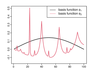
(b) Orthonormalized basis functions.

Figure 2: Motivation data and designed basis functions for Experiment 1.

Figure 2b presents the orthonormalized basis functions used in this experiment. Coefficients $\{\beta_{t,k}:k=1,2\}_{t=1}^{T}$ are generated from autoregressive models of order 1 (AR(1)) of the form $\beta_{t,k}=\theta_{k}\beta_{t-1,k}+\omega_{t,k}$. Select $\theta_{1}=0.8$ and $\omega_{t,1}\sim N(0,4)$ for $\{\beta_{t,1}\}_{t=1}^{T}$, while choosing $\theta_{2}=0.2$ and $\omega_{t,2}\sim N(0,0.01)$ for $\{\beta_{t,2}\}_{t=1}^{T}$. Combining the generated global and local features gives the true simulated process as $\mathcal{X}_{t}^{\text{TRUE}}=\beta_{t,1}\phi_{1}(u)+Z_{t}(u)=\beta_{t,1}\phi_{1}(u)+\beta_{t,2}\phi_{2}(u)$. Generate independent noise as $\varepsilon_{t}(u)=0.01B_{t}(u)$ with $B_{t}(u)$ i.i.d. standard Brownian motion $\{B_{t}(u)\}_{t=1}^{T}$. Finally, functional time series $\{\mathcal{X}_{t}(u)\}_{t=1}^{T}$ is calculated as $\mathcal{X}_{t}(u)=\mathcal{X}_{t}^{\text{TRUE}}+\varepsilon_{t}(u)$ for $u\in[0,1]$.

For each sample size $T\in\{25,50,100\}$, dynamic FPCA is applied to extract global features, with obtained results denoted by $\widehat{g}_{t}^{FPCA}(u)$. The BTW method, together with competing methods including the unified sparse and functional PCA (SFPCA) method of Allen & Weylandt (2019) and the two-way FPCA (TWFPCA) method of Huang et al. (2009), are applied to extract local features $\widehat{Z}_{t}(u)$ from FPCA residuals. SFPCA and TWFPCA are implemented with a grid search parameter selection approach provided by the MoMA package (Weylandt et al., 2018) in R (R Core Team, 2020). Estimation accuracy is assessed by relative squared error (RSE) defined in a simple Riemann sum as

$$\text{RSE}=\sum_{t=1}^{T}\frac{\left\lVert\mathcal{X}^{\text{TRUE}}_{t}-\widehat{g}_{t}^{\text{FPCA}}-\widehat{Z}_{t}\right\rVert^{2}}{\left\lVert\mathcal{X}^{\text{TRUE}}_{t}-\widehat{g}_{t}^{\text{FPCA}}\right\rVert^{2}}=\sum_{t=1}^{T}\sum_{i=1}^{100}\frac{\left|\mathcal{X}^{\text{TRUE}}_{t}(u_{i})-\widehat{g}_{t}^{\text{FPCA}}(u_{i})-\widehat{Z}_{t}(u_{i})\right|^{2}}{\left|\mathcal{X}^{\text{TRUE}}_{t}(u_{i})-\widehat{g}_{t}^{\text{FPCA}}(u_{i})\right|^{2}},$$

where $i=\{1,\ldots,100\}$ denote equally spaced discrete realizations over $[0,1]$. Given that the denominator of RSE corresponds to the reconstruction accuracy of the FPCA estimator, any estimation method with $\text{RSE}<1$ has a more accurate estimation performance than the conventional FPCA method. Moreover, the numerator of RSE is proportional to mean squared estimation error defined by $T^{-1}\sum_{t=1}^{T}\left\lVert\mathcal{X}_{t}(u)-\widehat{\mathcal{X}}_{t}(u)\right\rVert^{2}$. Thus, small RSE indicates an efficient local feature extraction method.

Table 1: Mean RSE and running time of various local feature extraction methods (standard errors in parentheses). The bold entries highlighting the best performing method for each setting.

Sample size		SFPCA	TWFPCA	BTW
$T=25$	RSE	0.687 (0.077)	0.749 (0.058)	0.663 (0.079)
	Time	15.462 (0.603)	21.085 (2.872)	0.154 (0.104)
$T=50$	RSE	0.659 (0.070)	0.737 (0.047)	0.639 (0.067)
	Time	34.288 (1.289)	20.206 (3.686)	0.143 (0.023)
$T=100$	RSE	0.649 (0.052)	0.731 (0.034)	0.629 (0.052)
	Time	89.555 (2.579)	21.089 (2.881)	0.244 (0.041)

Table 1 presents RSE averaged over 100 replications for three considered local feature extraction methods, together with computation time (in seconds) for a single iteration in R (R Core Team, 2020) on an AMD Ryzen Threadripper 1950X CPU at 3.40GHz. It can be seen that the BTW local feature extraction method consistently outperforms competing methods in estimation accuracy and computation efficiency. All three methods report RSE significantly less than 1, indicating that extracting local features after FPCA dramatically improves estimation accuracy. We note the existence of a greedy “coordinate-wise” Bayesian Information Criterion (BIC) optimization scheme by Allen & Weylandt (2019) that can significantly reduce computation time for the SFPCA and TWFPCA methods. However, in this experiment the BIC optimization approach produces RSEs around 1, suggesting that inappropriate penalty parameters are being selected. We present RSEs in relation to static FPCA in Appendix LABEL:app_b2 in the Supplementary document.

5.2 Experiment 2

Significant spikes of local features of functional time series are often visible in surface plots of long-run covariance functions. A good example of such data is spectroscopy of absorbance on samples of ground pork recorded on a Tecator infrared spectrometer in the region 850 to 1050 nm (Thodberg, 1996). Following Ferraty & Vieu (2006), we apply dynamic FPCA to 77 Tecator NIR spectroscopy spectra corresponding to samples with large fat content. Fitting the leading empirical scores associated with the leading functional components to an AR(1) model returns an estimated coefficient $0.2487$. Using analysis results of the Tecator data, we calibrate the data generating process for Experiment 2 by choosing $\phi_{1}(u)=\frac{1}{\sqrt{2\pi}}\exp{\{-\frac{u^{2}}{2}\}}$ and generating $\{\beta_{t,1}\}_{t=1}^{T}$ from $\beta_{t,1}=0.2487\beta_{t-1,1}+\omega_{t,1}$, where $\omega_{t,1}\sim N(0,1)$. To amplify bumps in covariances, local features are generated as

$$Z_{t}(u)=\begin{cases}0.5Z_{t-1}(u)+0.1B^{\ast}_{t}(u),&0.25\leq u<0.5\\ 0,&\text{elsewhere}\\ \end{cases},$$

where i.i.d. Brownian motion innovations $\{B^{\ast}_{t}(u),u\in[0.25,0.5]\}_{t=1}^{T}$ satisfy $B^{\ast}_{t}(0.25)=0$. Finally, independent noise is generated as $\varepsilon_{t}(u)=\sqrt{0.001}B_{t}(u)$ with $B_{t}(u)$ i.i.d. standard Brownian motion $\{B_{t}(u),u\in[0,1]\}_{t=1}^{T}$. Functional time series is computed as $\mathcal{X}_{t}(u)=\beta_{t}\phi_{1}(u)+Z_{t}(u)+\varepsilon_{t}(u)$ for $u\in[0,1]$.

For each simulated time series $\{\mathcal{X}_{t}(u)\}_{t=1}^{T}$, we apply the FPCA-BTW method to extract global and local features, and use the extracted features to reconstruct long-run covariance functions. The dynamic FPCA estimators are considered as comparison benchmarks. Estimation accuracy for covariance is assessed according to relative error (RE) given by

$$\text{RE}=\sqrt{\sum_{i=1}^{40}\sum_{j=1}^{40}\frac{\left|C(u_{i},s_{j})-\widehat{C}(u_{i},s_{j})\right|^{2}}{\left|C(u_{i},s_{j})\right|^{2}}},$$

where $C(u,s)$ is the theoretical long-run covariance function, and $\widehat{C}(u,s)$ is the reconstructed estimator using extracted features; $i,j=\{1,\ldots,40\}$ denote equally spaced grid points over $[0,1]$.

For each $T\in\{200,500,1000\}$, we replicate the experiment 100 times. Throughout the experiment, the empirical dimension of global features is determined to be $\widehat{K}=1$ by (10). Figure 3 shows that the FPCA-BTW method produces smaller reconstruction errors than the FPCA method. Hence, the extracted local features are tested to improve long-run covariance estimation accuracy. Finally, it can be easily observed that both FPCA and FPCA-BTW methods report smaller estimation errors when sample sizes increase.

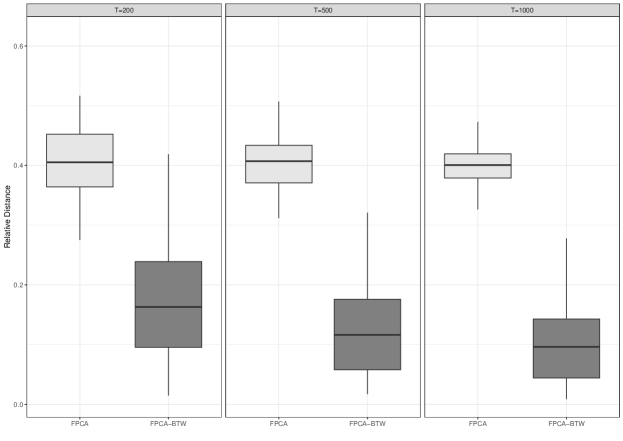
Figure 3: Relative errors of long-run covariance estimators.

Figure 4 visualizes the advantage of FPCA-BTW estimators in long-run covariance estimation when sample size $T=200$. Figure 4c presents the theoretical long-run covariance function that has a “pyramid-shaped bump” corresponding to local features $Z_{t}(u)$. Estimators depicted by Figure 4a fail to capture the “bump” of local features. In contrast, FPCA-BTW estimators successfully recover most information about local features in the presence of intentionally added noise. This experiment shows that local features are essential for the estimation of the long-run covariance function of functional time series.

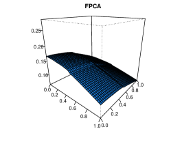
(a)

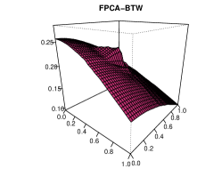
(b)

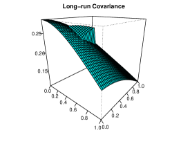
(c)

Figure 4: Surface plots of the mean long-run covariance estimators over 100 simulations obtained by FPCA (blue) and FPCA-BTW (red) for $T=200$, along with the true theoretical functions (cyan).

Monte Carlo experiments introduced in Section 5 prove that FPCA-BTW produces the best feature extraction performance among considered methods. We also design experiments to show that local features extracted by BTW help to improve point forecast accuracy, with details included in Appendix LABEL:app_b3 in the Supplementary document. In the next section, advantages of the FPCA-BTW method at feature extraction and forecasting functional time series are demonstrated using the empirical wood panel NIR spectroscopy data.

6 Empirical application

The wood panel NIR spectroscopy data illustrated in Figure 1 consists of spectra of absorbance (in negative base ten logarithm of the transmittance) recorded at wavelengths from 350 to 2500 nm in 1 nm intervals in a series of 72 experimental trials. Removing observations from 2301 to 2500 nm because of considerable noise gives $n=1951$ discrete realizations on each curve. Figure 1a indicates that raw spectra curves are contaminated by observational noise. Denoting the observed NIR absorbance values at wavelength $i$ in the $t$th curve as $Y_{t}(u_{i})$, the data can be expressed as

$$Y_{t}(u_{i})=\mathcal{X}_{t}(u_{i})+\varepsilon_{t}(u_{i}),\qquad i=1,\ldots,1951,\quad t=1,\ldots,72,$$

where $\mathcal{X}_{t}(u)$ is the true underlying smooth process, and $\varepsilon_{t}(u)$ is a random noise function. The smoothed functions displayed in Figure 1b are obtained by minimizing the penalized residual sum of squares (PENSSE) given by

$$\text{PENSSE}=\sum_{t=1}^{72}\sum_{i=1}^{1951}[\mathcal{X}_{t}(u_{i})-Y_{t}(u_{i})]^{2}+\lambda_{BS}\sum_{t=1}^{72}\int_{0}^{1}\frac{d^{2}\mathcal{X}_{t}(u)}{du^{2}}du,\qquad t=1,\ldots,72,\quad u\in[0,1],$$

where $\lambda_{BS}$ is a B-spline smoothing parameter selected by the fda.usc package in R (R Core Team, 2020) through generalized cross-validations. The functional KPSS test of Horváth et al. (2014) confirms that $\{\mathcal{X}_{t}(u)\}_{t=1}^{72}$ is stationary at the 5% significance level with a p-value of 0.053.

6.1 Feature extraction performance

We compare feature extraction performances of the FPCA-BTW method with competing sparse FPCA methods. The sample long-run covariance function for $\{\mathcal{X}_{t}(u)\}_{t=1}^{72}$ is computed following the procedures described in Section 3.1, and is presented in Figure 5. It can be seen that sharp spikes mainly occur between 1300 and 1900 nm, indicating that autocovariance functions at non-zero of lags $\{\mathcal{X}_{t}(u)\}_{t=1}^{72}$ also possess information exclusive to local features.

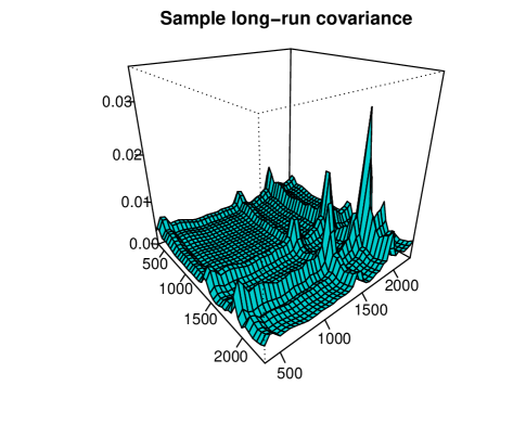
Figure 5: Sample long-run covariance function of smoothed wood panel NIR spectroscopy spectra.

Decomposing the sample long-run covariance operator reports the dimension of global features as $\widehat{K}=2$ by (10), and this result is confirmed by the empirical eigenvalues presented in Figure 1c. Using only global features we compute a long-run covariance estimator $\widehat{C}^{\text{FPCA}}(u,s)$. Next, we apply the BTW method, and also the SFPCA and TWFPCA methods mentioned in Section 5.1, to recover local features from dynamic FPCA residuals. With the extracted local features, we compute another estimator $\widehat{C}^{\text{local}}(u,s)$. The true process of NIR absorbance is not observable in practice. To assess effectiveness of various local feature extraction methods, a sample relative error is defined as

$$\text{Sample relative error}=\sqrt{\sum_{i=1}^{500}\sum_{j=1}^{500}\frac{\left|C^{\text{sample}}(u_{i},s_{j})-\widehat{C}^{\text{FPCA}}(u_{i},s_{j})-\widehat{C}^{\text{local}}(u_{i},s_{j})\right|^{2}}{\left|C^{\text{sample}}(u_{i},s_{j})-\widehat{C}^{\text{FPCA}}(u_{i},s_{j})\right|^{2}}},$$

where $i$ and $j$ denote equally spaced grid points over $[0,1]$. To accelerate the computation, we pick $n=500$ equally spaced grids on each $\mathcal{X}_{t}(u)$ and get sample relative errors of $0.255$, $0.386$ and $7.866e-5$ for the sparse FPCA method (Allen & Weylandt, 2019), the two-way FPCA method (Huang et al., 2009) and the BTW method, respectively. A sample RE close to 0 indicates that nearly all relevant information of the sample long-run covariance has been utilized in modeling the functional time series $\{\mathcal{X}_{t}(u)\}_{t=1}^{72}$. The obtained sample relative errors indicate that BTW is an optimal method for recovering sharp and highly localized features for functional data.

6.2 Forecasting performance

The forecasting performance of various global and local feature extraction methods are compared. First, the smoothed functions $\{\mathcal{X}_{t}(u)\}_{t=1}^{72}$ are divided into a training set $\{\mathcal{X}_{1}(u),\ldots,\mathcal{X}_{62}(u)\}$ and a testing set $\{\widehat{\mathcal{X}}_{63}(u),\ldots,\widehat{\mathcal{X}}_{72}(u)\}$. We apply the FPCA-BTW method to the training set, and use the obtained global and local features to make out-of-sample forecasts. Adopting the expanding window approach of Zivot & Wang (2006), in total we produce ten one-step-ahead forecasts, nine two-step-ahead forecasts, and so on, up to one 10-step-ahead forecast. Point forecasts obtained without considering local featires under the same expanding window setting serve as comparison benchmarks in this application.

To accelerate computation, we pick $n=500$ equally spaced grids on each $\mathcal{X}_{t}(u)$, and compute the mean absolute forecast error (MAFE) and the root mean squared forecast error (RMSFE) as

$$\text{MAFE}(h) =\frac{1}{500\times(11-h)}\sum^{10}_{\varsigma=h}\sum^{500}_{i=1}|\mathcal{X}_{62+\varsigma}(u_{i})-\widehat{\mathcal{X}}_{62+\varsigma|62+\varsigma-h}(u_{i})|,$$

$$\text{RMSFE}(h) =\sqrt{\frac{1}{500\times(11-h)}\sum^{10}_{\varsigma=h}\sum^{500}_{i=1}\left\{\mathcal{X}_{62+\varsigma}(u_{i})-\widehat{\mathcal{X}}_{62+\varsigma|62+\varsigma-h}(u_{i})\right\}^{2}},$$

where $\mathcal{X}_{62+\varsigma}(u_{i})$ represents the actual holdout sample at the $i$th wavelength of the $\varsigma$th curve, and $\widehat{\mathcal{X}}_{62+\varsigma}(u_{i})$ is the corresponding point forecasts. Averaging over ten forecast horizons, we obtain summary statistics given by

Median (MAFE) $$=\frac{1}{2}[\text{MAFE}(h=5)+\text{MAFE}(h=6)],$$

Mean (RMSFE) $$=\frac{1}{10}\sum^{10}_{h=1}\text{RMSFE}(h).$$

The median statistic is suitable for handling the absolute error MAFE while the mean statistic is good at handling the squared error RMSFE (Gneiting, 2011).

Point forecast evaluation results are reported in Tables 2. The forecasts constructed using only global features are shown in the columns with the heading “None”, with the remaining columns reporting forecasts produced with global and local features extracted by various methods. It can be easily seen that forecasts produced with local features are consistently more accurate. This result highlights the importance of incorporating local features in forecasting NIR spectroscopy spectra time series. Further, it can be seen that BTW consistently outperforms the competing methods in recovering local features relevant to forecasting. Thus, we recommend FPCA-BTW method in modeling and forecasting functional time series in practice. In addition, a comparison with point forecast evaluation results shown in Appendix LABEL:app_b2 indicates that dynamic FPCA produces more accurate point forecasts than static FPCA for the NIR spectroscopy data. This finding indicates that incorporating serial dependence carried by lagged NIR spectroscopy observations improves point forecast accuracy.

Table 2: Mean MAFEs and RMSFEs of point forecasts averaged over 100 replications. The bold entries highlight the feature extraction method with higher forecast accuracy.

	MAFE					RMSFE
$h$	None	BTW	SFPCA	TWFPCA		None	BTW	SFPCA	TWFPCA
1	0.482	0.430	0.450	0.450		0.870	0.837	0.841	0.846
2	0.502	0.449	0.473	0.475		0.882	0.841	0.852	0.857
3	0.528	0.475	0.498	0.502		0.910	0.872	0.878	0.884
4	0.537	0.486	0.511	0.516		0.918	0.870	0.884	0.891
5	0.543	0.491	0.513	0.518		0.939	0.891	0.902	0.910
6	0.580	0.533	0.556	0.566		0.988	0.938	0.951	0.962
7	0.598	0.552	0.575	0.592		1.016	0.959	0.976	0.994
8	0.645	0.596	0.627	0.650		1.041	0.972	1.003	1.030
9	0.704	0.646	0.685	0.717		1.115	1.044	1.072	1.105
10	0.593	0.531	0.548	0.577		1.144	1.082	1.109	1.133
Mean	0.571	0.519	0.544	0.556		0.982	0.931	0.942	0.961
Median	0.561	0.511	0.530	0.542		0.963	0.915	0.927	0.936

Table 2 shows that the FPCA-BTW method produces the most accurate point forecasts. Therefore, we do not further consider other competing feature extraction methods. To access the forecast uncertainty of FPCA-BTW method, we adapt the approach of Aue et al. (2015) and compute pointwise prediction intervals at the $100(1-a)\%$ nominal coverage probability. Technical details of interval forecasts are provided in Appendix LABEL:app_b3. Pointwise predictions intervals are evaluated using the interval score of Gneiting & Raftery (2007) given by

$$S_{a}\left[\widehat{\mathcal{X}}_{T+h}^{\text{lb}}(u_{i}),\widehat{\mathcal{X}}_{T+h}^{\text{ub}}(u_{i});\mathcal{X}_{T+h}(u_{i})\right] =\left[\widehat{\mathcal{X}}_{T+h}^{\text{ub}}(u_{i})-\widehat{\mathcal{X}}_{T+h}^{\text{lb}}(u_{i})\right]$$

$$+\frac{2}{a}\left[\widehat{\mathcal{X}}_{T+h}^{\text{lb}}(u_{i})-\mathcal{X}_{T+h}(u_{i})\right]\mathds{1}\left\{\mathcal{X}_{T+h}(u_{i})<\widehat{\mathcal{X}}_{T+h}^{\text{lb}}(u_{i})\right\}$$

$$+\frac{2}{a}\left[\mathcal{X}_{T+h}(u_{i})-\widehat{\mathcal{X}}_{T+h}^{\text{ub}}(u_{i})\right]\mathds{1}\left\{\mathcal{X}_{T+h}(u_{i})>\widehat{\mathcal{X}}_{T+h}^{\text{ub}}(u_{i})\right\},$$

where $\widehat{\mathcal{X}}_{T+h}^{\text{lb}}(u_{i})$ and $\widehat{\mathcal{X}}_{T+h}^{\text{ub}}(u_{i})$ denote lower and upper bounds of a symmetric $100(1-a)\%$ prediction interval, and the level of significance is customarily selected as $a=0.2$. To accelerate computation, we again pick $n=500$ equally spaced grids on each $\mathcal{X}_{t}(u)$. Averaging over different points in a curve and different forecast horizons, the mean interval score is defined as

$$\bar{S}_{\alpha}(h)=\frac{1}{500\times(11-h)}\sum^{10}_{\varsigma=h}\sum^{500}_{i=1}S_{a}\left[\widehat{\mathcal{X}}_{T+h}^{\text{lb}}(u_{i}),\widehat{\mathcal{X}}_{T+h}^{\text{ub}}(u_{i});\mathcal{X}_{T+h}(u_{i})\right],$$

where $S_{a}\left[\widehat{\mathcal{X}}_{T+h}^{\text{lb}}(u_{i}),\widehat{\mathcal{X}}_{T+h}^{\text{ub}}(u_{i});\mathcal{X}_{T+h}(u_{i})\right]$ denotes the interval score at the $\varsigma$th curve in the testing set. The interval scores summarized in Figure 6 confirm that incorporating the local features produces more accurate interval forecasts.

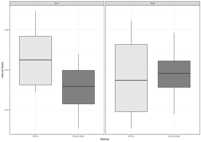
(a)

Figure 6: Scores of pointwise interval forecasts produced by FPCA method and FPCA-BTW method.

Moreover, extracting local features after retaining only one empirical functional component gives decent interval forecasts, which further highlights that the BTW method can effectively recover nearly all relevant information of functional data.

7 Conclusion

We propose a novel feature extraction method for functional time series. The proposed FPCA-BTW method improves the feature extraction performance of FPCA by recovering sharp, highly localized features from dimension reduction residuals. Local features extracted by BTW possess information of functional variations over particular short intervals within function domain, contributing to improved estimation results and more accurate forecasts. Theoretical properties of FPCA-BTW method are developed. Superior estimation and forecasting performances of FPCA-BTW estimators in finite samples are verified by Monte Carlo experiments and an empirical application to wood panel NIR spectroscopy data.

There are several ways in which the present paper can be further extended. First, this paper employed Cai’s (2002) parametric blockwise threshold approach to select wavelet coefficients. To make the proposed FPCA-BTW a nonparametric feature extraction method, the block size and threshold level at different resolution levels need to be selected based on characteristics of observations. A possible extension of the current method is adopting the data-driven block thresholding approach of Cai & Zhou (2009) to enhance extraction of local features. Moreover, this paper considered forecasting functional time series with extracted linear features. Non-linear extensions of functional regression, for example the continuously additive model of Müller et al. (2013), provide enhanced flexibility and structural stability. Another possible extension of the FPCA-BTW method may consider functional additive model (Müller & Yao, 2008) as the main dimension reduction tool. Since the inspirational work on functional manifold models by Donoho & Grimes (2005), functional manifold models have witnessed increasing contributions in methodology and applications (see, e.g., Lin & Yao, 2019).

References

- (1)
- Ahn & Horenstein (2013) Ahn, S. C. & Horenstein, A. R. (2013), ‘Eigenvalue ratio test for the number of factors’, Econometrica 81(3), 1203–1227.
-
Allen & Weylandt (2019)
Allen, G. I. & Weylandt, M. (2019), ‘Sparse and functional principal components analysis’, arXiv preprint
arXiv:1309.2895v5 .
https://arxiv.org/abs/1309.2895 - Andrews (1991) Andrews, D. (1991), ‘Heteroskedasticity and autocorrelation consistent covariant matrix estimation’, Econometrica 59(3), 817–858.
- Antoniadis (2007) Antoniadis, A. (2007), ‘Wavelet methods in statistics: Some recent developments and their applications’, Statistics Surveys 1, 16–55.
- Antoniadis & Fan (2001) Antoniadis, A. & Fan, J. (2001), ‘Regularization of wavelet approximations’, Journal of the American Statistical Association: Theory and Methods 96(455), 939–967.
- Aue et al. (2015) Aue, A., Norinho, D. D. & Hörmann, S. (2015), ‘On the prediction of stationary functional time series’, Journal of the American Statistical Association: Theory and Methods 110(509), 378–392.
- Bathia et al. (2010) Bathia, N., Yao, Q. & Ziegelmann, F. (2010), ‘Identifying the finite dimensionality of curve time series’, The Annals of Statistics 38(6), 3352–3386.
- Berkes et al. (2016) Berkes, I., Horváth, L. & Rice, G. (2016), ‘On the asymptotic normality of kernel estimators of the long run covariance of functional time series’, Journal of Multivariate Analysis 144, 150–175.
- Bosq (2000) Bosq, D. (2000), Linear Processes in Function Spaces, Lecture Notes in Statistics, New York.
- Bosq & Blanke (2007) Bosq, D. & Blanke, D. (2007), Inference and Prediction in Large Dimensions, John Wiley & Sons, West Sussex, England.
- Burns & Ciurczak (2007) Burns, D. A. & Ciurczak, E. W. (2007), Handbook of Near-Infrared Analysis, CRC press, Boca Raton, Florida.
- Cai (2002) Cai, T. T. (2002), ‘On block thresholding in wavelet regression: Adaptivity, block size, and threshold level’, Statistica Sinica 12, 1241–1273.
- Cai & Zhou (2009) Cai, T. T. & Zhou, H. H. (2009), ‘A data-driven block thresholding approach to wavelet estimation’, The Annals of Statistics 37(2), 569–595.
- Cao et al. (2018) Cao, J., Sang, P., Groves, K., Feng, M. & FPInnovations (2018), Stopping time detection in functional time series: An application to wood panel glue curing process. Joint Statistical Meetings 2018, Vancouver, Canada.
- Chiou (2012) Chiou, J.-M. (2012), ‘Dynamical functional prediction and classification with application to traffic flow prediction’, The Annals of Applied Statistics 6(4), 1588–1614.
- Daubechies (1992) Daubechies, I. (1992), Ten Lectures on Wavelets, Society for Industrial and Applied Mathematics, Philadelphia, PA.
- Donoho & Grimes (2005) Donoho, D. L. & Grimes, C. (2005), ‘Image manifolds which are isometric to euclidean space’, Journal of mathematical imaging and vision 23(1), 5–24.
- Donoho & Johnstone (1994) Donoho, D. L. & Johnstone, J. M. (1994), ‘Ideal spatial adaptation by wavelet shrinkage’, Biometrika 81(3), 425–455.
- Fan et al. (2013) Fan, J., Liao, Y. & Mincheva, M. (2013), ‘Large covariance estimation by thresholding principal orthogonal complements’, Journal of the Royal Statistical Society: Series B (Statistical Methodology) 75(4), 603–680.
- Ferraty & Vieu (2006) Ferraty, F. & Vieu, P. (2006), Nonparametric Functional Data Analysis: Theory and Practice, Springer Science & Business Media, New York.
- Gellar et al. (2014) Gellar, J. E., Colantuoni, E., Needham, D. M. & Crainiceanu, C. M. (2014), ‘Variable-domain functional regression for modeling ICU data’, Journal of the American Statistical Association: Applications and Case Studies 109(508), 1425–1439.
- Gneiting (2011) Gneiting, T. (2011), ‘Making and evaluating point forecasts’, Journal of the American Statistical Association: Review Article 106(494), 746–762.
- Gneiting & Raftery (2007) Gneiting, T. & Raftery, A. E. (2007), ‘Strictly proper scoring rules, prediction and estimation’, Journal of the American Statistical Association: Review Article 102(477), 359–378.
- Grossmann & Morlet (1984) Grossmann, A. & Morlet, J. (1984), ‘Decomposition of hardy functions into square integrable wavelets of constant shape’, SIAM Journal on Mathematical Analysis 15(4), 723–736.
- Hall & Hooker (2016) Hall, P. & Hooker, G. (2016), ‘Truncated linear models for functional data’, Journal of the Royal Statistical Society: Series B (Statistical Methodology) 78(3), 637–653.
- Hall & Vial (2006) Hall, P. & Vial, C. (2006), ‘Assessing the finite dimensionality of functional data’, Journal of the Royal Statistical Society (Series B) 68(4), 689–705.
- Hörmann et al. (2015) Hörmann, S., Kidziński, Ł. & Hallin, M. (2015), ‘Dynamic functional principal components’, Journal of the Royal Statistical Society: Series B (Statistical Methodology) 77(2), 319–348.
- Hörmann & Kokoszka (2010) Hörmann, S. & Kokoszka, P. (2010), ‘Weakly dependent functional data’, The Annals of Statistics 38(3), 1845–1884.
- Horváth & Kokoszka (2012) Horváth, L. & Kokoszka, P. (2012), Inference for Functional Data with Applications, Vol. 200, Springer Science & Business Media, New York.
- Horváth et al. (2014) Horváth, L., Kokoszka, P. & Rice, G. (2014), ‘Testing stationarity of functional time series’, Journal of Econometrics 179(1), 66–82.
- Horváth et al. (2016) Horváth, L., Rice, G. & Whipple, S. (2016), ‘Adaptive bandwidth selection in the long run covariance estimator of functional time series’, Computational Statistics & Data Analysis 100, 676–693.
- Huang et al. (2009) Huang, J. Z., Shen, H. & Buja, A. (2009), ‘The analysis of two-way functional data using two-way regularized singular value decompositions’, Journal of the American Statistical Association: Theory and Methods 104(488), 1609–1620.
- Hyndman & Shang (2009) Hyndman, R. J. & Shang, H. L. (2009), ‘Forecasting functional time series (with discussions)’, Journal of the Korean Statistical Society 38(3), 199–221.
- Hyndman & Shang (2010) Hyndman, R. J. & Shang, H. L. (2010), ‘Rainbow plots, bagplots, and boxplots for functional data’, Journal of Computational and Graphical Statistics 19(1), 29–45.
- Johnstone & Lu (2009) Johnstone, I. M. & Lu, A. Y. (2009), ‘On consistency and sparsity for principal components analysis in high dimensions’, Journal of the American Statistical Association: Theory and Methods 104(486), 682–693.
- Klepsch & Klüppelberg (2017) Klepsch, J. & Klüppelberg, C. (2017), ‘An innovations algorithm for the prediction of functional linear processes’, Journal of Multivariate Analysis 155, 252–271.
- Klepsch et al. (2017) Klepsch, J., Klüppelberg, C. & Wei, T. (2017), ‘Prediction of functional ARMA processes with an application to traffic data’, Econometrics and Statistics 1, 128–149.
- Kokoszka & Reimherr (2013) Kokoszka, P. & Reimherr, M. (2013), ‘Determining the order of the functional autoregressive model’, Journal of Time Series Analysis 34(1), 116–129.
- Lam & Yao (2012) Lam, C. & Yao, Q. (2012), ‘Factor modeling for high-dimensional time series: inference for the number of factors’, The Annals of Statistics 40(2), 694–726.
- Lam et al. (2011) Lam, C., Yao, Q. & Bathia, N. (2011), ‘Estimation of latent factors for high-dimensional time series’, Biometrika 98(4), 901–918.
- Li et al. (2020) Li, D., Robinson, P. M. & Shang, H. L. (2020), ‘Long-range dependent curve time series’, Journal of the American Statistical Association: Theory and Methods 115(530), 957–971.
- Lin & Yao (2019) Lin, Z. & Yao, F. (2019), ‘Intrinsic riemannian functional data analysis’, The Annals of Statistics 47(6), 3533–3577.
- Mallat (1989) Mallat, S. G. (1989), ‘A theory for multiresolution signal decomposition: the wavelet representation’, IEEE Transactions on Pattern Analysis and Machine Intelligence 11(7), 674–693.
- Mallat (2009) Mallat, S. G. (2009), A Wavelet Tour of Signal Processing: the Sparse Way, 3rd edn, Elsevier/Academic Press, Amsterdam; Boston.
- Meyer (1992) Meyer, Y. (1992), Wavelets and operators, Vol. 1, Cambridge university press, Cambridge.
- Müller et al. (2013) Müller, H.-G., Wu, Y. & Yao, F. (2013), ‘Continuously additive models for nonlinear functional regression’, Biometrika 100(3), 607–622.
- Müller & Yao (2008) Müller, H.-G. & Yao, F. (2008), ‘Functional additive models’, Journal of the American Statistical Association: Theory and Methods 103(484), 1534–1544.
- Ogden (1997) Ogden, T. (1997), Essential Wavelets for Statistical Applications and Data Analysis, Springer, Boston.
- Parzen (1957) Parzen, E. (1957), ‘On consistent estimates of the spectrum of a stationary time series’, The Annals of Mathematical Statistics 28(2), 329–348.
- Politis & Romano (1996) Politis, D. N. & Romano, J. P. (1996), ‘On flat-top kernel spectral density estimators for homogeneous random fields’, Journal of Statistical Planning and Inference 51(1), 41–53.
-
R Core Team (2020)
R Core Team (2020), R: A Language and
Environment for Statistical Computing, R Foundation for Statistical
Computing, Vienna, Austria.
http://www.R-project.org/ - Rice & Shang (2017) Rice, G. & Shang, H. L. (2017), ‘A plug-in bandwidth selection procedure for long-run covariance estimation with stationary functional time series’, Journal of Time Series Analysis 38(4), 591–609.
- Shang (2019) Shang, H. L. (2019), ‘Dynamic principal component regression: Application to age-specific mortality forecasting’, ASTIN Bulletin: The Journal of the IAA 49(3), 619–645.
- Shang & Hyndman (2011) Shang, H. L. & Hyndman, R. J. (2011), ‘Nonparametric time series forecasting with dynamic updating’, Mathematics and Computers in Simulation 81(7), 1310–1324.
- Solo (2001) Solo, V. (2001), ‘Regularization of wavelet approximations: Discussion’, Journal of the American Statistical Association: Theory and Methods 96(455), 963–964.
- Strang (1989) Strang, G. (1989), ‘Wavelets and dilation equations: A brief introduction’, SIAM review 31(4), 614–627.
- Thodberg (1996) Thodberg, H. H. (1996), ‘A review of Bayesian neural networks with an application to near infrared spectroscopy’, IEEE Transactions on Neural Networks 7(1), 56–72.
-
Weylandt et al. (2018)
Weylandt, M., Allen, G. & Liao, L. (2018), MoMA: MoMA - Modern Multivariate Analysis in R.
R package version 0.1.
https://github.com/DataSlingers/MoMA - Zhao et al. (2012) Zhao, Y., Ogden, R. T. & Reiss, P. T. (2012), ‘Wavelet-based lasso in functional linear regression’, Journal of Computational and Graphical Statistics 21(3), 600–617.
- Zivot & Wang (2006) Zivot, E. & Wang, J. (2006), Modeling Financial Time Series with S-PLUS, Springer, New York.