The Generalization of the Periodic Orbit Dividing Surface in Hamiltonian Systems with three or more degrees of freedom - I

Abstract

We present a method that generalizes the periodic orbit dividing surface construction for Hamiltonian systems with three or more degrees of freedom. We construct a torus using as a basis a periodic orbit and we extend this to a $2n-2$ dimensional object in the $2n-1$ dimensional energy surface. We present our methods using benchmark examples for two and three degree of freedom Hamiltonian systems to illustrate the corresponding algorithm for this construction. Towards this end we use the normal form quadratic Hamiltonian system with two and three degrees of freedom. We found that the periodic orbit dividing surface can provide us the same dynamical information as the dividing surface constructed using normally hyperbolic invariant manifolds. This is significant because, in general, computations of normally hyperbolic invariant manifolds are very difficult in Hamiltonian systems with three or more degrees of freedom. However, our method avoids this computation and the only information that we need is the location of one periodic orbit.

1 Introduction

In this paper we construct dividing surfaces from periodic orbits in Hamiltonian systems with three or more degrees of freedom. This generalises the periodic orbit dividing surface construction developed in Pechukas & McLafferty [1973]; Pechukas & Pollak [1977]; Pollak & Pechukas [1978].

A dividing surface (at a fixed value of energy) is a surface that has one less dimension than that of the energy surface of a Hamiltonian system. This surface has the property of no-recrossing and orientability. For our purposes the significance of orientability is that a surface has two well-defined sides. We underline the fact that we must not confuse the no-recrossing property of the dividing surfaces with the Poincaré recurrence in the case of closed and bounded energy surfaces. In the case of Poincaré recurrence the trajectories starting from an initial point in the phase space (included the dividing surfaces) will eventually return close to the initial position. This is independent from the choice of the dividing surface. Dividing surfaces play a central role in Wigner’s vision for transition state theory Wigner [1938]; Waalkens et al. [2007], which is a widely used theory for understanding chemical reaction dynamics.

In Hamiltonian systems with two degrees of freedom the phase space is four-dimensional and the energy surface is three-dimensional. This means that the dividing surface is two-dimensional surface embedded in the three-dimensional energy surface. This dividing surface is constructed using periodic orbits (Pechukas [1981], Pollak [1985]) that are 1-dimensional closed curves.

Until now, the construction of a dividing surface in Hamiltonian systems with three or more degrees can be done from the Normally Hyperbolic Invariant Manifold (NHIMs) Wiggins et al. [2001]; Uzer et al. [2002]; Wiggins [2016]. The phase space is $2n$-dimensional and the energy surface is $2n-1$ dimensional surface. The periodic orbit is one-dimensional and it has not enough dimensions to construct a dividing surface using the method that we use in Hamiltonian systems with two degrees of freedom. The Normally Hyperbolic Invariant Manifold is a $2n-3$ dimensional structure in the $2n-1$ dimensional energy surface. The dimensions of this object can guarantee the construction of a $2n-2$ dimensional structure embedded in the $2n-1$ dimensional energy surface Waalkens et al. [2007], Waalkens & Wiggins [2010]. The construction of a Dividing surface from the NHIM can be done through the computation of the Poincaré-Birkhoff normal form (NF) theory near an index-one saddle. By this method we obtain explicit formulas for the Normally Hyperbolic Invariant Manifolds and Dividing surfaces (Wiggins et al. [2001], Uzer et al. [2002], Waalkens et al. [2007], Toda [2003], Komatsuzaki & Berry [2003]). But in many situations this method is difficult to apply and it requires extensive algebraic calculations.

In this paper we propose a new method to construct dividing surfaces without to know the NHIM, avoiding the extensive and difficult calculations through the Normal Form theory. We use the periodic orbit, that is actually a 1-dimensional submanifold of the Normally Hyperbolic Invariant Manifold, as a starting point to construct a dividing surface. We give an introduction and pseudocode of our algorithm in the general context of the Hamiltonian Systems with $n$ degrees of freedom in the section 2. We describe our algorithm for the case of the Hamiltonian systems with two and three degrees of freedom in the sections 3 and 4 respectively. In these sections, we apply our algorithm to a quadratic normal form Hamiltonian system with two and three degrees of freedom and we compare the periodic orbit dividing surfaces that are constructed from our algorithm with the dividing surfaces that are constructed from the NHIM. We choose this system because we have analytical formulas for the periodic orbits and the NHIM (Ezra & Wiggins [2018]). This allows us to compute the dividing surfaces from the periodic orbits and the NHIM and to compare these results (see sections 3 and 4). Then we present the algorithm in the general case of a Hamiltonian system with $n$ degrees of freedom (see section 5). Finally, we present our conclusions in the last section.

2 The skeleton of the Algorithm - Pseudocode

In this section we present a method for the construction of a periodic orbit dividing surface in Hamiltonian systems with three or more degrees of freedom. This method generalizes the classical periodic orbit dividing surface that is valid only in Hamiltonian systems with two degrees of freedom. We consider the general case of Hamiltonian systems with $n$ degrees of freedom with potential energy function $V(x_{1},x_{2},...,x_{n})$ with $n\geq 2$ of the form :

$$T+V(x_{1},x_{2},...,x_{n})=E$$

where $T$ is the kinetic energy.

$$T=p_{x_{1}}^{2}/2m_{1}+p_{x_{2}}^{2}/2m_{2}+...+p_{x_{n}}^{2}/2m_{n}$$

where $p_{x_{1}},p_{x_{2}},...p_{x_{n}}$ are the momenta and $m_{1},m_{2},..m_{n}$ are the corresponding masses.

A basic assumption of our algorithm is that there exists a two dimensional (2D) subspace in the $2n$ dimensional (D) phase space in which the periodic orbit can be represented by a closed curve. With this assumption the algorithm has two versions.

First version.

In this version we assume that the periodic orbit is represented by a closed curve in a 2D subspace of the phase space that it is not a subspace of the configuration space (for example in the $(x_{1},p_{x_{1}})$ space). In other words, the 2D subspace in this version has one coordinate corresponding to a configuration space variable and the other corresponding to a phase space variable. We refer to this space as the extended configuration space.

Second version.

In this version we assume that the periodic orbit can be represented as a closed curve in a 2D subspace of the configuration space. For example the 2D subspace is described by the coordinates $(x_{1},x_{2})$.

In this section, we describe the two versions of the algorithm for the construction of the dividing surfaces if we know the location of one periodic orbit. For this reason we present a diagram (pseudocode) that describes the two versions of the algorithm (Fig. 1). We see in this diagram that we check first if the periodic orbit satisfies the conditions that are necessary in order to use one of two versions or not. Firstly, we check if the periodic orbit is valid for the second version. If this is true then we follow the steps of the second version (see Fig. 1) otherwise we check the validity of the first version of the algorithm. If the periodic orbit satisfies the conditions for the first version then we follow the steps of this version (see Fig. 1) otherwise we must use another method.

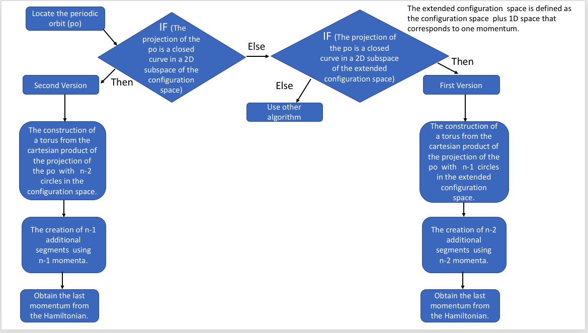
Figure 1: The pseudocode for the algorithm.

3 The Algorithm for Hamiltonian systems with two degrees of freedom

In the previous section we described the difference between the two versions of our algorithm for the construction of dividing surfaces and the circumstances when we use one or the other version. Now, we describe in detail the two versions of our algorithm (for $n=2$) in the case of Hamiltonian systems with two degrees of freedom with potential energy function $V(x,y)$:

$$p_{x}^{2}/2m_{1}+p_{y}^{2}/2m_{2}+V(x,y)=E$$

where $p_{x},p_{y}$ are the momenta and $m_{1},m_{2}$ the corresponding masses.
The algorithm for Hamiltonian systems with two degrees of freedom comprises the next two algorithms that correspond to the first and second version of our algorithm. The application of the second version in Hamiltonian systems with two degrees of freedom give us the same algorithm as the classical algorithm for periodic orbit dividing surfaces (see Pechukas & McLafferty [1973]; Pechukas & Pollak [1977]; Pollak & Pechukas [1978]; Pechukas & Pollak [1979]; Pollak [1985] and for more details see Ezra & Wiggins [2018]). We describe the two versions of the algorithm in the first two subsections and we present an application of the algorithm to the case of a quadratic normal form Hamiltonian with two degrees of freedom in the third subsection.

3.1 The first version of the algorithm

The first version of the algorithm is:

1. Locate an unstable periodic orbit PO for a fixed value of Energy $E$.

2. Project the PO into the configuration space and consider a 2D subspace of the phase space in which the projection of the periodic orbit is a closed curve (for example in the $(y,p_{y})$ space).

3. From the projection of the periodic orbit in the configuration space, we construct a torus that is generated by the Cartesian product of a circle with small radius and the projection of the periodic orbit in a 2D subspace of the phase space (for example in the $(y,p_{y})$ space). Actually it is topologically equivalent to the Cartesian product of two circles $S^{1}\times S^{1}$. This is a two-dimensional torus. This can be achieved through the construction of one circle around every point of the periodic orbit in the 2D subspace of the 3D subspace of the phase space. For example we compute a circle (with a fixed radius r) in the plane $(x,y)$ around every point of the periodic orbit in the 3D space $(x,y,p_{y})$. The goal of this step is to include all coordinates of the configuration space in this torus.

   $$y_{1,i,j1}=y_{0,i}+rcos(\theta_{j1})$$

   $$x_{1,i,j1}=x_{0,i}+rsin(\theta_{j1})$$

   $$p_{y,1,i,j1}=p_{y,0,i}$$ (4)

   $(x_{0,i},y_{0,i},p_{y,0,i}),i=1,...N$ are the points of the periodic orbit in the 3D subspace $(x,y,p_{y})$. We have the angle $\theta_{j1}=j1\frac{2\pi}{n_{1}}$ with $j1=1,...,n_{1}$ for the circle that we need for the construction of the torus. $x_{1,i,j1},y_{1,i,j1},p_{y,1,i,j1}$ with $i=1,...,N$ and $j1=1,...,n_{1}$ are the points of the torus that is constructed from the Cartesian product of projection of the periodic orbit in the 2D subspace $(y,p_{y})$ and a circle in the $(x,y)$ space in the 3D space $(x,y,p_{y})$.

4. For each point $x_{1,i,j1},y_{1,i,j1},p_{y,1,i,j1}$ on this torus we can calculate the $p_{x,1,i,j1}$ by solving the following equation for a fixed value of energy (Hamiltonian) $E$:

   $$V(x_{1,i,j1},y_{1,i,j1})+\frac{p_{x,1,i,j1}^{2}}{2m_{1}}+\frac{p_{y,1,i,j1}^{2}}{2m_{2}}=E$$

Dimensionality and Topology: This algorithm constructs a torus as the product of the closed curve that represents the projection of the periodic orbit (1D object) in a 2D subspace of the phase space with one circle in the 3D energy surface. This torus is a 2-dimensional. Then we obtain the value of the last momentum from the Hamiltonian of the system.

3.2 The second version of the algorithm

The second version of the algorithm is:

1. Locate an unstable periodic orbit PO for a fixed value of Energy $E$.

2. $(x_{0,i},y_{0,i}),i=1,...N$ are the points of the periodic orbit in the 2D configuration space $(x,y)$. This is a closed curve in a 2D subspace. Actually it is topologically equivalent with a circle.

3. For each point $x_{0,i},y_{0,i}$ of the periodic orbit we must calculate the $p_{x,0,i}^{max}$ and $p_{x,0,i}^{min}$ by solving the following equation for a fixed value of energy (Hamiltonian) $E$ with $p_{y}=0$:

   $$V(x_{0,i},y_{0,i})+\frac{p_{x,0,i}^{2}}{2m_{1}}=E$$

   and we find the maximum and minimum values $p_{x,0,i}^{max}$ and $p_{x,0,i}^{min}$. We choose points $p_{x,0,i}$ in the interval $p_{x,0,i}^{min}\leq p_{x,0,i}\leq p_{x,0,i}^{max}$. These points can be uniformly distributed in this interval.

4. Now for every point $x_{0,i},y_{0,i},p_{x,0,i}$ we must calculate the $p_{y,0,i}$ by solving the following equation for a fixed value of energy (Hamiltonian) E:

   $$V(x_{0,i},y_{0,i})+\frac{p_{x,0,i}^{2}}{2m_{1}}+\frac{p_{y,0,i}^{2}}{2m_{2}}=E$$

Dimensionality and Topology: This algorithm give us an 1-dimensional object (a circle or ellipse) as the projection of the periodic orbit (1D object) in the configuration space. Then we sample the third variable (one of the momenta) in the interval between its maximum and minimum value. Actually we create an additional 1D segment and we increase the dimensionality of the initial object (a circle or ellipse), from 1 to 2 dimensions, which is embedded in the 3D energy surface. Then we obtain the value of the last momentum from the Hamiltonian of the system.

3.3 Application of the algorithm to the Quadratic Normal Form Hamiltonian System with two degrees of freedom

Now we will apply the algorithm to the system that is described in subsection 3.3.1. In this system the reaction occurs when $x$ changes sign Ezra & Wiggins [2018]. The dividing surfaces for this system using the classical algorithm have been computed (see for example Ezra & Wiggins [2018]). In this subsection we will use our algorithm to compute the dividing surfaces. This can be done if we choose the condition $x=0$ that is actually a 3-dimensional surface in the four dimensional phase space. This will be applied in our algorithm. We will construct a dividing surface from the periodic orbit PO that is a circle in the plane $(y,p_{y})$ (see subsection 3.3.2). The first version of our algorithm is valid for this periodic orbit because we have the combination of one coordinate of the configuration space and one momentum (see for details the diagram in section 2). We underline the fact that because one of the coordinates of the configuration space is $x=0$ (in our case) we have not the need to construct a two-dimensional torus. This means that the first version of the algorithm is simplified and we construct the torus using the one circle that is the projection of the periodic orbit.

3.3.1 Hamiltonian Model

The quadratic normal form Hamiltonian system near an index-one saddle Wiggins [2016] is described by the following Hamiltonian:

$$H=\frac{\lambda}{2}(p_{x}^{2}-x^{2})+\frac{\omega}{2}(p_{y}^{2}+y^{2})$$

with $\lambda>0,\omega>0$ and

$$H_{1}=\frac{\lambda}{2}(p_{x}^{2}-x^{2})$$

$$H_{2}=\frac{\omega}{2}(p_{y}^{2}+y^{2})$$

The equations of motion are:

$$\dot{x}=\frac{\partial H}{\partial p_{x}}=\lambda p_{x}$$

$$\dot{p}_{x}=-\frac{\partial H}{\partial x}=\lambda x$$

$$\dot{y}=\frac{\partial H}{\partial p_{y}}=\omega p_{y}$$

$$\dot{p}_{y}=-\frac{\partial H}{\partial y}=-\omega y$$

The Hamiltonian functions $H_{1}$ and $H_{2}$ are uncoupled. The phase space of these two subsystems can be studied separately. In this system we can distribute the total energy between each mode. The ($x,p_{x},y,p_{y})=(0,0,0,0)$) for E=0 is an one-index saddle point of the full system.

In this system the reaction occurs when the $x$ coordinate changes sign (for $H_{1}>0$). We choose the condition $x=0$ (Ezra & Wiggins [2018]) to define a three-dimensional surface in the four-dimensional phase space. From the equations 3.3.1 we have that $H_{2}\geq 0$ and finally $H=H_{1}+H_{2}\equiv E>0$. The energy surface is:

$$\frac{\lambda}{2}(p_{x}^{2}-x^{2})+\frac{\omega}{2}(p_{y}^{2}+y^{2})=E$$

the intersection of $x=0$ with this surface is:

$$\frac{\lambda}{2}p_{x}^{2}+\frac{\omega}{2}(p_{y}^{2}+y^{2})=E$$

This is the Dividing surface (a two-sphere) that can be constructed by the NHIM (see for more details in Wiggins [2016] and Ezra & Wiggins [2018]). The NHIM is the unstable periodic orbit in Hamiltonian systems with two degrees of freedom. We call this periodic orbit as PO. The equator of this dividing surface is given by $p_{x}=0$ and we have:

$$\frac{\omega}{2}(p_{y}^{2}+y^{2})=E\qquad PO$$

This equation represents the periodic orbit (PO) that is a circle in the plane $(y,p_{y})$.In the next section we will construct, using the algorithm 1, a two dimensional dividing surface using this periodic orbit.

3.3.2 PO-Dividing Surface

We apply the first version (see the introduction of this section) of our algorithm to the PO (see 3.3.1):

1. The periodic orbit 1 is given by 3.3.1 for every fixed value $E$.

2. The periodic orbit is a circle and it lies on a plane ($(y,p_{y})$. The radius of this circle is $\sqrt{\frac{2E}{\omega}}$.

3. As we described in the introduction of this section the dividing surface is embedded in the surface $x=0$ and this means that we have not the need to construct a two-dimensional torus. This means that this step will be simplified and we will construct 1-dimensional torus using one circle that is the projection of the periodic orbit in the $(y,p_{y})$ plane. The equation of this torus is the equation 3.3.1.

4. Step 4 is carried out naturally in this case (with $x=0$). We compute $p_{x}$ from the Hamiltonian.

   no-recrossing property:

   $$p_{x}=\sqrt{\frac{2}{\lambda}(H_{1}+H_{2}-\frac{\omega}{2}(p_{y}^{2}+y^{2}))}\qquad p_{x}>0\qquad Forward\quad DS$$

   $$p_{x}=-\sqrt{\frac{2}{\lambda}(H_{1}+H_{2}-\frac{\omega}{2}(p_{y}^{2}+y^{2}))}\qquad p_{x}<0\qquad Backward\quad DS$$

The new DS that is constructed has the no-recrossing property because $\dot{x}=\lambda p_{x}$. This is exactly the same dividing surface that we obtain from the classical algorithm of Pechukas [1981],[Pollak, 1985] (see equations 12 in Ezra & Wiggins [2018]).

4 The Algorithm for Hamiltonian systems with three degrees of freedom

In the section 2 we described the difference between the two versions of our algorithm for the construction of dividing surfaces and when we use both versions. Now, we describe in detail the two versions of our algorithm (for $n=3$) in the case of Hamiltonian systems with three degrees of freedom with a potential energy $V(x,y,z)$:

$$p_{x}^{2}/2m_{1}+p_{y}^{2}/2m_{2}+p_{z}^{2}/2m_{3}+V(x,y,z)=E$$

where $p_{x},p_{y},p_{z}$ are the momenta and $m_{1},m_{2},m_{3}$ the corresponding masses.
When we apply the two versions of the algorithm in Hamiltonian systems with three degrees of freedom we produce two algorithms, one algorithm for each version. We describe the two versions of the algorithm in the first two subsections and we present an application of the algorithm to the case of a quadratic normal form Hamiltonian with three degrees of freedom in the third subsection.

4.1 The first version of the algorithm

The first version of the algorithm is:

1. Locate an unstable periodic orbit PO for a fixed value of Energy $E$.

2. Project the PO into the configuration space and we consider a 2D subspace of the phase space in which the projection of the periodic orbit is a closed curve (for example in the $(y,p_{y})$ space).

3. From the projection of the periodic orbit in the configuration space, we construct a torus that is generated by the Cartesian product of 2 circles with small radius and the projection of the periodic orbit in a 2D subspace of the phase space (for example in the $(y,p_{y})$ space). Actually it is topologically equivalent with the Cartesian product of three circles $S^{1}\times S^{1}\times S^{1}$. This is a three-dimensional torus (Hypertorus). This can be achieved through the construction of one circle around every point of the periodic orbit in the 2D subspace of a 4D subspace of the phase space. For example we compute a circle (with a fixed radius r) in the plane $(x,y)$ around every point of the periodic orbit in the 4D subspace $(x,y,z,p_{y})$. Then we construct a new circle around every point of the previous structure in the 4D subspace $(x,y,z,p_{y})$ of the phase space. This can be done computing a circle (with a fixed radius r) in the plane $(y,z)$. The goal of this step is to include all coordinates of the configuration space in this torus.

   $$y_{1,i,j1}=y_{0,i}+rcos(\theta_{j1})$$

   $$x_{1,i,j1}=x_{0,i}+rsin(\theta_{j1})$$

   $$z_{1,i,j1}=z_{0,i}$$

   $$p_{y,1,i,j1}=p_{y,0,i}$$ (16)

   $$y_{2,i,j1,j2}=y_{1,i,j1}+rcos(\theta_{j2})$$

   $$z_{2,i,j1,j2}=z_{1,i,j1}+rsin(\theta_{j2})$$

   $$x_{2,i,j1,j2}=x_{1,i,j1}$$

   $$p_{y,2,i,j1,j2}=p_{y,1,i,j1}$$ (17)

   $(x_{0,i},y_{0,i},z_{0,i},p_{y,0,i}),i=1,...N$ are the points of the periodic orbit in the 4D subspace $(x,y,z,p_{y})$. We have the angle $\theta_{j1}=j1\frac{2\pi}{n_{1}}$ with $j1=1,...,n_{1}$ for the first circle and $\theta_{j2}=j2\frac{2k\pi}{n_{1}}$ with $j2=1,...,n_{1}$ for the second circle that we need for the construction of the torus.

   $x_{1,i,j1},y_{1,i,j1},z_{1,i,j1},p_{y,1,i,j1}$ with $i=1,...,N$ and $j1=1,...,n_{1}$ are the points of the torus that is constructed from the Cartesian product of projection of the periodic orbit in the 2D subspace $(y,p_{y})$ and a circle in the $(x,y)$ space in the 4D space $(x,y,z,p_{y})$. $x_{2,i,j1,j2},y_{2,i,j1,j2},z_{2,i,j1,j2},p_{y,2,i,j1,j2}$ with $i=1,...,N$, $j1=1,...,n_{1}$ and $j2=1,...,n_{1}$ are the points of the torus that is constructed from the Cartesian product of the projection of the periodic orbit in the 2D subspace $(y,p_{y})$, a circle in the $(x,y)$ space and a circle in the $(y,z)$ space in the 4D space $(x,y,z,p_{y})$.

4. For each point $x_{2,i,j1,j2},y_{2,i,j1,j2},z_{2,i,j1,j2},p_{y,2,i,j1,j2}$ on this torus we must calculate the $p_{x,2,i,j1,j2}^{max}$ and $p_{x,2,i,j1,j2}^{min}$ by solving the following equation for a fixed value of energy (Hamiltonian) $E$ with $p_{z}=0$:

   $$V(x_{2,i,j1,j2},y_{2,i,j1,j2},z_{2,i,j1,j2})+\frac{p_{x,2,i,j1,j2}^{2}}{2m_{1}}+\frac{p_{y,2,i,j1,j2}^{2}}{2m_{2}}=E$$

   and we find the maximum and minimum values $p_{x,2,i,j1,j2}^{max}$ and $p_{x,2,i,j1,j2}^{min}$. We choose points $p_{x,2,i,j1,j2}$ with $j2=1,...,n_{1}$ in the interval $p_{x,2,i,j1,j2}^{min}\leq p_{x,2,i,j1,j2}\leq p_{x,2,i,j1,j2}^{max}$. These points can be uniformly distributed in this interval. Then we obtain the value $p_{z,2,i,j1,j2}$ from the Hamiltonian:

   $$V(x_{2,i,j1,j2},y_{2,i,j1,j2},z_{2,i,j1,j2})+\frac{p_{x,2,i,j1,j2}^{2}}{2m_{1}}+\frac{p_{y,2,i,j1,j2}^{2}}{2m_{2}}+\frac{p_{z,2,i,j1,j2}^{2}}{2m_{3}}=E$$

Dimensionality and Topology: This algorithm constructs a torus as the product of the closed curve that represents the projection of the periodic orbit (1D object) in a 2D subspace with two circles in the 4D subspace of the 5D energy manifold. This torus is a 3-dimensional (hypertorus). Then we sample the fifth variable (one of the momenta) in the interval between its maximum and minimum value. Actually we create an additional 1D segment and we increase the dimensionality of the initial torus, from 3 to 4 dimensions, which is embedded in the 5D energy surface. Then we obtain the value of the last momentum from the Hamiltonian of the system.

4.2 The second version of the algorithm

The second version of the algorithm is:

1. Locate an unstable periodic orbit PO for a fixed value of Energy $E$.

2. Project the PO into the configuration space and we consider a 2D subspace of the configuration space in which the projection of the periodic orbit is a closed curve (for example in the $(x,y)$ space).

3. We construct a torus that is generated by the Cartesian product of one circle with small radius and the projection of the periodic orbit in a 2D subspace of the configuration space (for example in the $(x,y)$ space). Actually it is the Cartesian product of two circles $S^{1}\times S^{1}$. This is a two-dimensional torus. This can be achieved through the construction of one circle around every point of the periodic orbit in the 2D subspace of a 3D subspace of the phase space. For example we compute a circle (with a fixed radius r) in the plane $(y,z)$ around every point of the periodic orbit in the 3D subspace $(x,y,z)$.

   The points of the torus that we constructed are:

   $$y_{1,i,j1}=y_{0,i}+rcos(\theta_{j1})$$

   $$z_{1,i,j1}=z_{0,i}+rsin(\theta_{j1})$$

   $$x_{1,i,j1}=x_{0,i}$$ (20)

   $(x_{0,i},y_{0,i},z_{0,i}),i=1,...N$ are the points of the periodic orbit in the 3D configuration space $(x,y,z)$. We have the angle $\theta_{j1}=j1\frac{2\pi}{n_{1}}$ with $j1=1,...,n_{1}$ for the circle that we need for the construction of the torus.

   $x_{1,i,j1},y_{1,i,j1},z_{1,i,j1}$ with $i=1,...,N$ and $j1=1,...,n_{1}$ are the points of the torus that is constructed from the Cartesian product of projection of the periodic orbit in the 2D subspace $(x,y)$ and a circle in the $(y,z)$ space in the 3D space $(x,y,z)$.

4. For each point $x_{1,i,j1},y_{1,i,j1},z_{1,i,j1}$ on this torus we must calculate the $p_{x,1,i,j1}^{max}$ and $p_{x,1,i,j1}^{min}$ by solving the following equation for a fixed value of energy (Hamiltonian) $E$ with $p_{y}=p_{z}=0$:

   $$V(x_{1,i,j1},y_{1,i,j1},z_{1,i,j1})+\frac{p_{x,1,i,j1}^{2}}{2m_{1}}=E$$

   and we find the maximum and minimum values $p_{x,1,i,j1}^{max}$ and $p_{x,1,i,j1}^{min}$. We choose points $p_{x,1,i,j1}$ with $j1=1,...,n_{1}$ in the interval $p_{x,1,i,j1}^{min}\leq p_{x,1,i,j1}\leq p_{x,1,i,j1}^{max}$. These points can be uniformly distributed in this interval.

5. Now for every point $x_{1,i,j1},y_{1,i,j1},z_{1,i,j1},p_{x,1,i,j1}$ we must calculate the $p_{y,1,i,j1}^{max}$ and $p_{y,1,i,j1}^{min}$ by solving the following equation for a fixed value of energy (Hamiltonian) $E$ with $p_{z}=0$:

   $$V(x_{1,i,j1},y_{1,i,j1},z_{1,i,j1})+\frac{p_{x,1,i,j1}^{2}}{2m_{1}}+\frac{p_{y,1,i,j1}^{2}}{2m_{2}}=E$$

   We choose points $p_{y,1,i,j1}$ with $j1=1,...,n_{1}$ in the interval $p_{y,1,i,j1}^{min}\leq p_{y,1,i,j1}\leq p_{y,1,i,j1}^{max}$. These points can be uniformly distributed in this interval. Then we obtain the value $p_{z,1,i,j1}$ from the Hamiltonian:

   $$V(x_{1,i,j1},y_{1,i,j1},z_{1,i,j1})+\frac{p_{x,1,i,j1}^{2}}{2m_{1}}+\frac{p_{y,1,i,j1}^{2}}{2m_{2}}+\frac{p_{z,1,i,j1}^{2}}{2m_{3}}=E$$

Dimensionality and Topology: This algorithm constructs a torus as the product of the closed curve that represents the projection of the periodic orbit (1D object) in a 2D subspace with one circle in the configuration space. This torus is a 2-dimensional. Then we sample the fourth variable (one of the momenta) in the interval between its maximum and minimum value. Actually we create an additional 1D segment and we increase the dimensionality of the initial torus, from 2 to 3 dimensions, which is embedded in the 4D subspace of the 5D energy surface. Then we sample the fifth variable (one of the other two momenta) in the interval between its maximum and minimum value. This means that we create an additional 1D segment and we increase the dimensionality of the initial torus, from 3 to 4 dimensions, which is embedded in the 5D energy surface. Then we obtain the value of the last momentum from the Hamiltonian of the system.

4.3 Application of the algorithms in the Quadratic Normal Form Hamiltonian System with three degrees of freedom

Now we will apply the algorithm to the system that is described in subsection 4.3.1. In this system the reaction occurs when $x$ changes sign Ezra & Wiggins [2018]. This can be done if we choose the condition $x=0$ that is actually a 5-dimensional surface in the six dimensional phase space. This will be applied in our algorithms (in this way, we consider the intersection of the four dimensional structure that is obtained by our algorithm with $x=0$). Firstly we will construct a dividing surface from the periodic orbit PO1 that is a circle in the plane $(y,p_{y})$ (see subsection 4.3.2). Then we will do the same for the periodic orbit PO2 that is a circle in the plane $(z,p_{z})$ (see subsection 4.3.3). In this case we will use version 1 of the algorithm because the periodic orbits are closed curves in the 2D subspaces of the phase space that consist of a combination of a coordinate of the configuration space with one momentum (see the conditions for the choice between the first and second version in the section 2) . We underline the fact that because one of the coordinates of the configuration space is $x=0$ (in our case) we have not the need to construct a three-dimensional torus. This means that the first version of the algorithm is simplified and we construct the torus using the Cartesian product of one circle (not two circles) with the projection of the periodic orbit.

4.3.1 Hamiltonian Model

The quadratic normal form Hamiltonian system near an index-one saddle Wiggins [2016] is described by the following Hamiltonian:

$$H=\frac{\lambda}{2}(p_{x}^{2}-x^{2})+\frac{\omega_{2}}{2}(p_{y}^{2}+y^{2})+\frac{\omega_{3}}{2}(p_{z}^{2}+z^{2})$$

with $\lambda>0,\omega_{2}>0,\omega_{3}>0$ and

$$H_{1}=\frac{\lambda}{2}(p_{x}^{2}-x^{2})$$

$$H_{2}=\frac{\omega_{2}}{2}(p_{y}^{2}+y^{2})$$

$$H_{3}=\frac{\omega_{3}}{2}(p_{z}^{2}+z^{2})$$

The equations of motion are:

$$\dot{x}=\frac{\partial H}{\partial p_{x}}=\lambda p_{x}$$

$$\dot{p}_{x}=-\frac{\partial H}{\partial x}=\lambda x$$

$$\dot{y}=\frac{\partial H}{\partial p_{y}}=\omega_{2}p_{y}$$

$$\dot{p}_{y}=-\frac{\partial H}{\partial y}=-\omega_{2}y$$

$$\dot{z}=\frac{\partial H}{\partial p_{z}}=\omega_{3}p_{z}$$

$$\dot{p}_{z}=-\frac{\partial H}{\partial z}=-\omega_{3}z$$

The Hamiltonian functions $H_{1}$ ,$H_{2}$ and $H_{3}$ are uncoupled. The phase space of these three subsystems can be studied separately. In this system we can distribute the total energy between each mode. The ($x,p_{x},y,p_{y},z,p_{z})=(0,0,0,0,0,0)$) for E=0 is an one-index saddle point of the full system.

In this system the reaction occurs when the $x$ coordinate changes sign (for $H_{1}>0$). We choose the condition $x=0$ (Ezra & Wiggins [2018]) to define a five-dimensional surface in the six-dimensional phase space. From the equations 4.3.1 we have that $H_{2}\geq 0$ and $H_{3}\geq 0$ and finally $H=H_{1}+H_{2}+H_{3}\equiv E>0$. The energy surface is:

$$\frac{\lambda}{2}(p_{x}^{2}-x^{2})+\frac{\omega_{2}}{2}(p_{y}^{2}+y^{2})+\frac{\omega_{3}}{2}(p_{z}^{2}+z^{2})=E$$

the intersection of $x=0$ with this surface is:

$$\frac{\lambda}{2}p_{x}^{2}+\frac{\omega_{2}}{2}(p_{y}^{2}+y^{2})+\frac{\omega_{3}}{2}(p_{z}^{2}+z^{2})=E$$

This is the dividing surface (a four-sphere) that can be constructed by the NHIM (see for more details in Wiggins [2016] and Ezra & Wiggins [2018]). The equator of this dividing is given by $p_{x}=0$ and we have:

$$\frac{\omega_{2}}{2}(p_{y}^{2}+y^{2})+\frac{\omega_{3}}{2}(p_{z}^{2}+z^{2})=E\qquad NHIM$$

The previous equation represents the NHIM. The intersection of the NHIM with $z=0$ is given by the following equation:

$$\frac{\omega_{3}}{2}p_{z}^{2}+\frac{\omega_{2}}{2}(p_{y}^{2}+y^{2})=E$$

The equator of the NHIM is given by $p_{z}=0$ and we have the following equation:

$$\frac{\omega_{2}}{2}(p_{y}^{2}+y^{2})=E\qquad PO1$$

This equation represents the periodic orbit (PO1) that is a circle in the plane $(y,p_{y})$.

The intersection of the NHIM (see the equation 4.3.1) with $y=0$ is given by the following equation:

$$\frac{\omega_{2}}{2}p_{y}^{2}+\frac{\omega_{3}}{2}(p_{z}^{2}+z^{2})=E$$

The equator of the NHIM is given by $p_{y}=0$ and we have the following equation:

$$\frac{\omega_{3}}{2}(p_{z}^{2}+z^{2})=E\qquad PO2$$

This equation represents the periodic orbit (PO2) that is a circle in the plane $(z,p_{z})$. In the next subsections we will construct dividing surfaces using the periodic orbits PO1 and PO2.

4.3.2 PO1-Dividing Surface

We begin by applying the first version of our algorithm to the PO1 (see 4.3.1):

1. The PO1 is given by 4.3.1 for every fixed value $E$.

2. The periodic orbit is a circle and it lies on a plane ($(y,p_{y})$. The radius of this circle is $\sqrt{\frac{2E}{\omega_{2}}}$.

3. We construct a torus in the 3D subspace $(y,p_{y},z)$ using the product of the circle of the periodic orbit and a circle with small fixed radius $r>0$. The equation of this torus (with $x=0$):

   $$(\sqrt{p_{y}^{2}+y^{2}}-\sqrt{\frac{2E}{\omega_{2}}})^{2}+z^{2}=r^{2}$$

4. Step 4 is carried out naturally in this case (with $x=0$). We compute the $p_{z}^{max}$ and $p_{z}^{min}$. We sample points in the interval $[p_{z}^{min},p_{z}^{max}]$. For every point in the previous interval we obtain the $p_{x}$ coordinate from the Hamiltonian.

   no-recrossing property:

   from the equation 3 we have:

   $$z^{2}=r^{2}-(\sqrt{p_{y}^{2}+y^{2}}-\sqrt{\frac{2E}{\omega_{2}}})^{2}$$

   from the equation 4.3.1 (for a fixed value of energy $E$, the numerical value of the Hamiltonian and for $x=0$) we have:

   $$\frac{\lambda}{2}p_{x}^{2}=E-\frac{\omega_{2}}{2}(p_{y}^{2}+y^{2})-\frac{\omega_{3}}{2}(p_{z}^{2}+z^{2})$$

   The equation 4 through the equation 4 and using that $E=H_{1}+H_{2}+H_{3}$ with $H_{2}=\frac{\omega_{2}}{2}(p_{y}^{2}+y^{2})$ (from equation 4.3.1) we have:

   $$\frac{\lambda}{2}p_{x}^{2}=H_{1}+H_{3}-\frac{\omega_{3}}{2}p_{z}^{2}+\frac{\omega_{3}}{2}(\sqrt{p_{y}^{2}+y^{2}}-\sqrt{\frac{2E}{\omega_{2}}})^{2}-\frac{\omega_{3}}{2}r^{2}$$

   From equation 4.3.1 we have that $H_{3}-\frac{\omega_{3}}{2}p_{z}^{2}>0$. We have also that the quantity $\frac{\omega_{3}}{2}(\sqrt{p_{y}^{2}+y^{2}}-\sqrt{\frac{2E}{\omega_{2}}})^{2}\geq 0$ is always positive. This means that the condition that we must have for the equation 4 is:

   $$H_{1}-\frac{\omega_{3}}{2}r^{2}\geq 0$$

   This implies that:

   $$r\leq\sqrt{\frac{2H_{1}}{\omega_{3}}}$$

   In practise this means that we must choose a small radius r. Using this condition we have for the dividing surface :

   $$p_{x}=\sqrt{\frac{2}{\lambda}(H_{1}+H_{3}-\frac{\omega_{3}}{2}p_{z}^{2}+\frac{\omega_{3}}{2}(\sqrt{p_{y}^{2}+y^{2}}-\sqrt{\frac{2E}{\omega_{2}}})^{2}-\frac{\omega_{3}}{2}r^{2})}\qquad p_{x}>0\qquad Forward\quad DS$$

   $$p_{x}=-\sqrt{\frac{2}{\lambda}(H_{1}+H_{3}-\frac{\omega_{3}}{2}p_{z}^{2}+\frac{\omega_{3}}{2}(\sqrt{p_{y}^{2}+y^{2}}-\sqrt{\frac{2E}{\omega_{2}}})^{2}-\frac{\omega_{3}}{2}r^{2})}\qquad p_{x}<0\qquad Backward\quad DS$$

The new DS that is constructed has the no-recrossing property because $\dot{x}=\lambda p_{x}$.

4.3.3 PO2-Dividing Surface

Now we apply the first version of our algorithm to the PO2 (see 4.3.1):

1. The PO2 is given by 4.3.1 for every fixed value $E$.

2. The periodic orbit is a circle and it lies on a plane $(z,p_{z})$. The radius of this circle is $\sqrt{\frac{2E}{\omega_{3}}}$.

3. We construct a torus in the 3D subspace $(z,p_{z},y)$ using the product of the circle of the periodic orbit and a circle with small fixed radius $r_{1}>0$. The equation of this torus (with $x=0$):

   $$(\sqrt{p_{z}^{2}+z^{2}}-\sqrt{\frac{2E}{\omega_{3}}})^{2}+y^{2}=r_{1}^{2}$$

4. Step 4 is carried out naturally in this case (with $x=0$). We compute the $p_{y}^{max}$ and $p_{y}^{min}$. We sample points in the interval $[p_{y}^{min},p_{y}^{max}]$. For every point in the previous interval we obtain the $p_{x}$ coordinate from the Hamiltonian.

   no-recrossing property:

   from the equation 3 we have:

   $$y^{2}=r_{1}^{2}-(\sqrt{p_{z}^{2}+z^{2}}-\sqrt{\frac{2E}{\omega_{3}}})^{2}$$

   from the equation 4.3.1 (for a fixed value of energy $E$, the numerical value of the Hamiltonian) we have:

   $$\frac{\lambda}{2}p_{x}^{2}=E-\frac{\omega_{2}}{2}(p_{y}^{2}+y^{2})-\frac{\omega_{3}}{2}(p_{z}^{2}+z^{2})$$

   The equation 4 through the equation 4 and using that $E=H_{1}+H_{2}+H_{3}$ with $H_{3}=\frac{\omega_{3}}{2}(p_{z}^{2}+z^{2})$ (from equation 4.3.1) we have:

   $$\frac{\lambda}{2}p_{x}^{2}=H_{1}+H_{2}-\frac{\omega_{2}}{2}p_{y}^{2}+\frac{\omega_{2}}{2}(\sqrt{p_{z}^{2}+z^{2}}-\sqrt{\frac{2E}{\omega_{3}}})^{2}-\frac{\omega_{2}}{2}r_{1}^{2}$$

   From equation 4.3.1 we have that $H_{2}-\frac{\omega_{2}}{2}p_{y}^{2}>0$. We have also that the quantity $\frac{\omega_{2}}{2}(\sqrt{p_{y}^{2}+y^{2}}-\sqrt{\frac{2E}{\omega_{3}}})^{2}\geq 0$ is always positive. This means that the condition that we must have for the equation 4 is:

   $$H_{1}-\frac{\omega_{2}}{2}r_{1}^{2}\geq 0$$

   This implies that:

   $$r_{1}\leq\sqrt{\frac{2H_{1}}{\omega_{2}}}$$

   In practise this means that we must choose a small radius $r_{1}$. Using this condition we have for the dividing surface :

   $$p_{x}=\sqrt{\frac{2}{\lambda}(H_{1}+H_{2}-\frac{\omega_{2}}{2}p_{y}^{2}+\frac{\omega_{2}}{2}(\sqrt{p_{z}^{2}+z^{2}}-\sqrt{\frac{2E}{\omega_{3}}})^{2}-\frac{\omega_{2}}{2}r_{1}^{2})}\qquad p_{x}>0\qquad Forward\quad DS$$

   $$p_{x}=-\sqrt{\frac{2}{\lambda}(H_{1}+H_{2}-\frac{\omega_{2}}{2}p_{y}^{2}+\frac{\omega_{2}}{2}(\sqrt{p_{z}^{2}+z^{2}}-\sqrt{\frac{2E}{\omega_{3}}})^{2}-\frac{\omega_{2}}{2}r_{1}^{2})}\qquad p_{x}<0\qquad Backward\quad DS$$

The new DS that is constructed has the no-recrossing property because $\dot{x}=\lambda p_{x}$.

4.3.4 The structure and the comparison of the Dividing surfaces

In this section we constructed the dividing surfaces from the periodic orbits PO1 and PO2 and from the Normally Hyperbolic Invariant Manifold (NHIM) of the quadratic normal form Hamiltonian (see section 4.3.1) for ($\lambda=1,\omega_{2}=\sqrt{2},\omega_{3}=1$). These values were used from Ezra & Wiggins [2018]. The value of the energy was $E=14,H_{1}=4$. We computed the dividing surfaces from the periodic orbits PO1 and PO2 using the algorithms and analytical formulas of the previous subsections (see subsections 4.3.2 and 4.3.3). The dividing surface from the NHIM is obtained using the algorithm and analytical formulae from Ezra & Wiggins [2018].

We begin by constructing the dividing surface from the periodic orbit 1 (PO1) in three different cases. For this purpose we construct a torus (using as a starting point the periodic orbit PO1- see subsection 4.3.2) that is the cartesian product of the periodic orbit with a circle. The maximum radius of this circle is $Rmax=\sqrt{\frac{2H_{1}}{\omega_{3}}}$ (see the equation 4). We used three cases for the construction of a torus using a circle with small radius r ($r=Rmax/20$), a circle with larger radius r ($r=Rmax/2$) and a circle with the maximum radius r ($r=Rmax$).

Next we construct the dividing surface from the periodic orbit 2 (PO2). For this purpose we construct a torus (using as a starting point the periodic orbit PO2- see subsection 4.3.3) that is the cartesian product of the periodic orbit with a circle. The maximum radius $r_{1}$ of this circle is $R1max=\sqrt{\frac{2H_{1}}{\omega_{2}}}$ (see the equation 4). In this paper we used the maximum radius $r_{1}$ for the construction of the PO2 dividing surface. Finally we construct the dividing surface from the NHIM.

All dividing surfaces as we mentioned in the previous sections are 4 dimensional structures in the energy surface. All dividing surfaces have $x=0$ (as we mentioned in the previous section and we obtain the $p_{x}$ coordinate from the Hamiltonian) and this is the reason that we studied the structure of the dividing surfaces in the 4-dimensional space $(y,z,p_{y},p_{z})$.

We studied first the structure of these dividing surfaces and then we compare them:

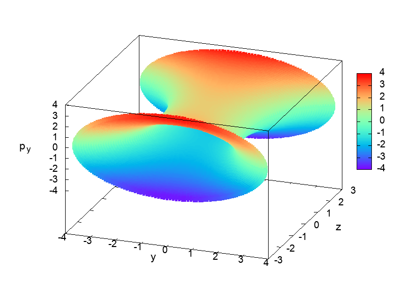
Figure 5: The 3D projection $(y,z,p_{y})$ of the dividing surface which is constructed from the periodic orbit PO1 with the associated torus to have r=Rmax. The color indicates the values of the third dimension.The viewpoint is in spherical coordinates is $(60^{o},20^{o})$.

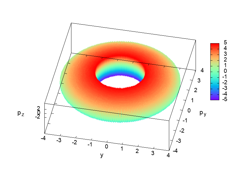
Figure 6: The 3D projection $(y,p_{y},p_{z})$ of the dividing surface which is constructed from the periodic orbit PO1 with the associated torus to have r=Rmax. The color indicates the values of the third dimension.The viewpoint is in spherical coordinates is $(20^{o},12^{o})$.

1. The structure of the dividing surfaces: All dividing surfaces that are constructed from the periodic orbits have similar structure in the 4-dimensional space $(y,z,p_{y},p_{z})$. In this subsection, we choose one representative example of these surfaces, the dividing surface from PO1 with the associated torus to have r=Rmax. We depict this surface in all 3D projections of the 4-dimensional space $(y,z,p_{y},p_{z})$. This surface is constructed as a torus. This topology is very obvious (as we can see in Fig. 6) in $(y,p_{y},p_{z})$ projection. This torus has also an hyperbolic structure that is represented as an hyperboloid (as we can see in Fig. 5) in $(y,z,p_{y})$ projection and hyperbolic box structure (as we can see in Fig. 4) in $(y,z,p_{z})$ and $(z,p_{y},p_{z})$ projections. This means that the dividing surfaces that are constructed from periodic orbits are hyperbolic tori in the 4-dimensional space $(y,z,p_{y},p_{z})$.

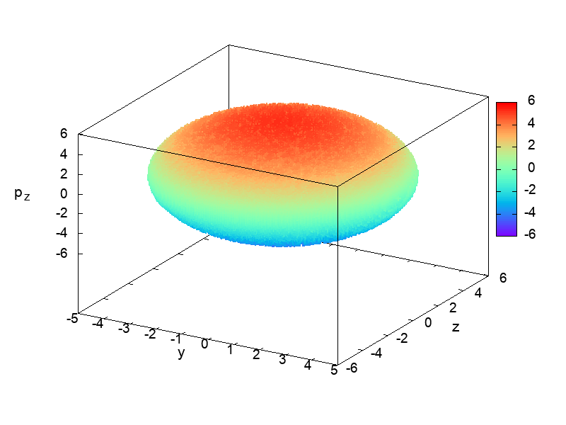
Figure 7: The 3D projection $(y,z,p_{z})$ of the dividing surface which is constructed from the NHIM. The color indicates the values of the third dimension.The viewpoint is in spherical coordinates is $(30^{o},60^{o})$.

   The dividing surface that is constructed from the NHIM is an ellipsoid in all 3D projections of the 4-dimensional space $(y,z,p_{y},p_{z})$. (as we can see for example in $(y,z,p_{z})$ projection in Fig.7). This means that this dividing surface is an ellipsoid in the 4-dimensional space.

2. Comparison of Dividing surfaces: In Fig. 2 we compare the dividing surfaces that are constructed from the periodic orbit PO1. For this reason we use the 2D projections $(y,z)$, $(y,p_{y})$ and $(z,p_{z})$. Using these projections we can understand if one dividing surface is larger in the $y$ or $z$ or $p_{y}$ or $p_{z}$ direction. This means that these 2D projections are enough for the comparison of different dividing surfaces without the use of the other 2D projections $(y,p_{z})$, $(z,p_{y})$ and $(p_{y},p_{z})$. As we can see in the Fig. 2 the dividing surface with associated torus with $r=Rmax/20$ has similar length in the y-direction with the other two dividing surfaces. The dividing surfaces form a hyperbolic box in the $(y,z)$ projection that grows up with the increase of the radius of the one circle that is needed for the construction of dividing surfaces (Fig. 2). The increase of the radius increases the extension of the dividing surfaces in the z-direction. This is the reason that the hyperbolic box of the dividing surface with $r=Rmax/20$ is smaller than this of the dividing surface with $r=Rmax/2$ and this is smaller than the hyperbolic box of the dividing surface with $r=Rmax$. In Fig. 2 we see that the dividing surfaces form a ring structure in the $(y,p_{y})$ projection and an elliptic structure in the $(z,p_{z})$ with increasing thickness as we increase the radius of the circle that is needed for the construction of the dividing surfaces (see Fig. 2). As we increase the radius of the circle that generates the torus that is the basis for the construction of a periodic orbit dividing surface, this surface becomes more elongated in the $p_{z}$ and $z$ directions (Fig. 2).

   We compare the PO2 dividing surface with the PO1 dividing surface, both of them associated with the torus with the maximum $r$ and $r_{1}$ respectively. We compare the two cases of the dividing surfaces in Figs. 2. We observe that the PO1 dividing surface is more elongated on the y-axis and the PO2 dividing surface is more elongated on the z-axis (Fig. 2). Furthermore, the PO2 dividing surface form a ring structure in the $(z,p_{z})$ and not in the $(y,p_{y})$ as the PO1 dividing surface. In addition, the PO2 dividing surface form an elliptic structure in the $(y,p_{y})$ and not in the $(z,p_{z})$ as the PO1 dividing surface. All these differences are because of the fact that the PO1 is a circle in the $(y,p_{y})$ plane and PO2 is a circle in the $(z,p_{z})$ plane. This means that the combination of these dividing surfaces give us the dynamical information for every direction in the configuration space for a small area of interest (the neighbourhood of the periodic orbits).

   We compare the dividing surface from the NHIM with the dividing surfaces from the PO1 and PO2, both of them associated with the torus with the maximum $r$ and $r_{1}$ respectively. We observe in Fig. 2 that the dividing surface from PO1 and PO2 have the same range of values with the dividing surface from the NHIM (Fig.3) in the $p_{y}$-direction and $p_{z}$-direction. But the PO1 dividing surface and the PO2 dividing surface have smaller range of values than this of the dividing surface from the NHIM (Fig. 3) in the $z$-directon and $y$-direction respectively. This means that the dividing surfaces from PO1 and PO2 are subsets of the dividing surface from the NHIM.

We give an example of trajectories that have initial conditions on one from dividing surfaces that we constructed from the periodic orbits PO1 and PO2 and we integrate them for 2 time units. We used as example the dividing surface that is constructed from the PO1 that is constructed by a torus with small radius $r=Rmax/20$ (Fig. 8). We observe that this structure has as a central region a box with a tiny thickness and at the edges it has many sheets in the configuration space. The structure of this surface is similar with these that we obtained if the trajectories have initial conditions on other dividing surfaces that are constructed from the same or the other periodic orbit PO2.

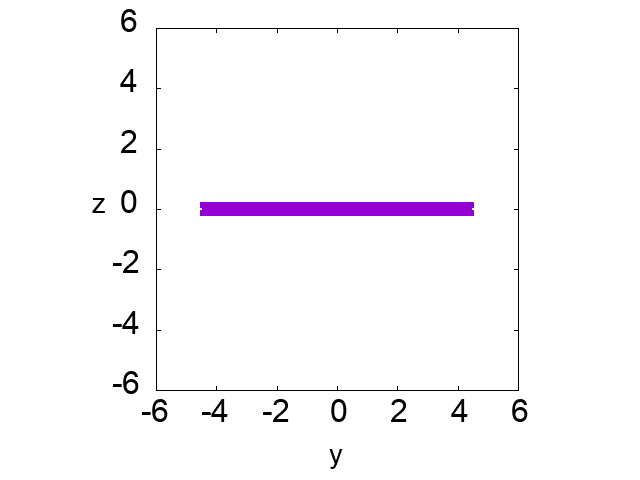
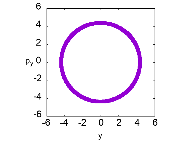
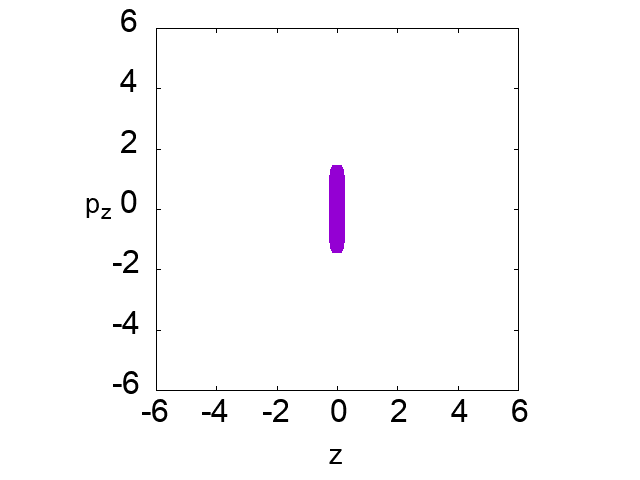
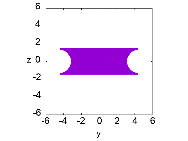
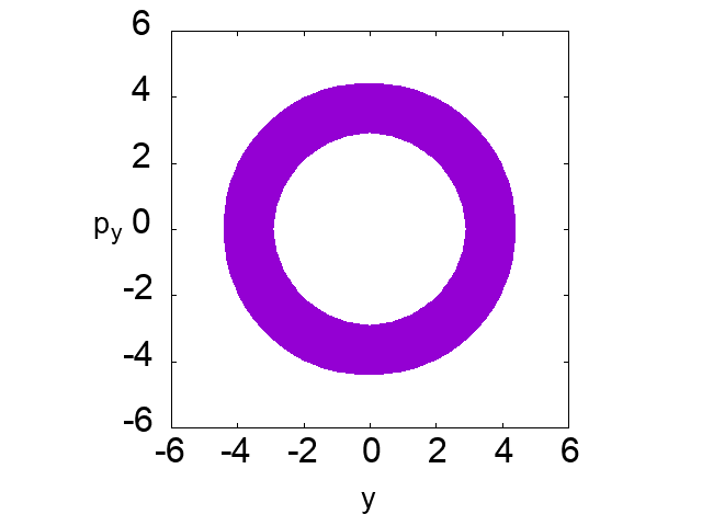
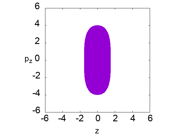
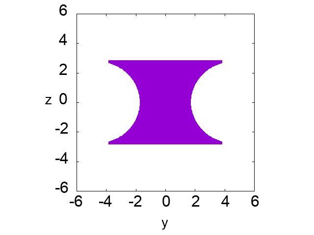
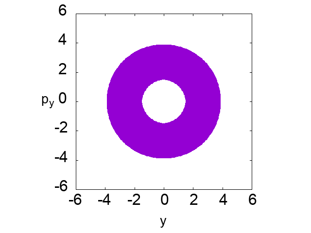
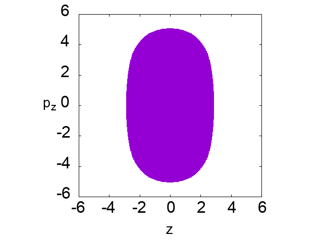
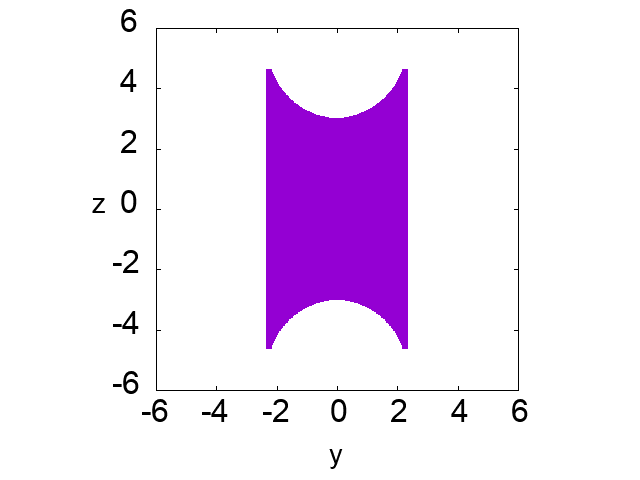
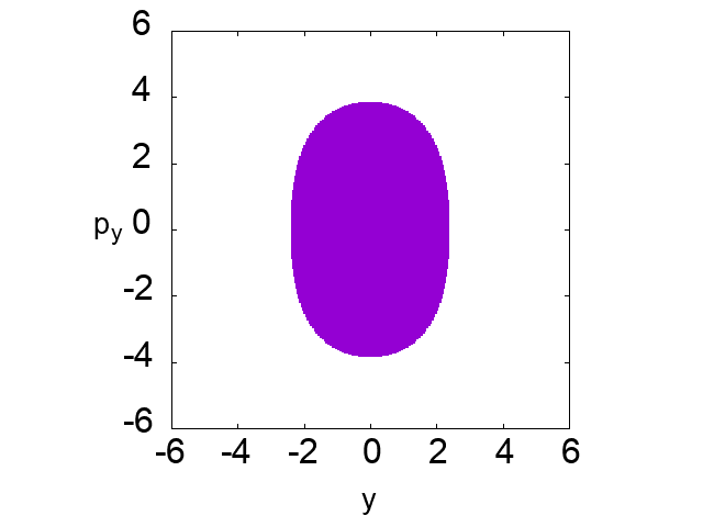
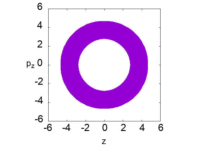
Figure 2: 2D projections of periodic orbit dividing surfaces in $(y,z)$ (first column), $(y,p_{y})$ (second column) and $(z,p_{z})$ (third column) subspaces of the phase space. The dividing surfaces are constructed from the periodic orbit PO1 with the associated torus to have r=Rmax/20 (first row), r=Rmax/2 (second row) and r=Rmax (third row) and from the periodic PO2 with the associated torus to have r=Rmax (fourth row).

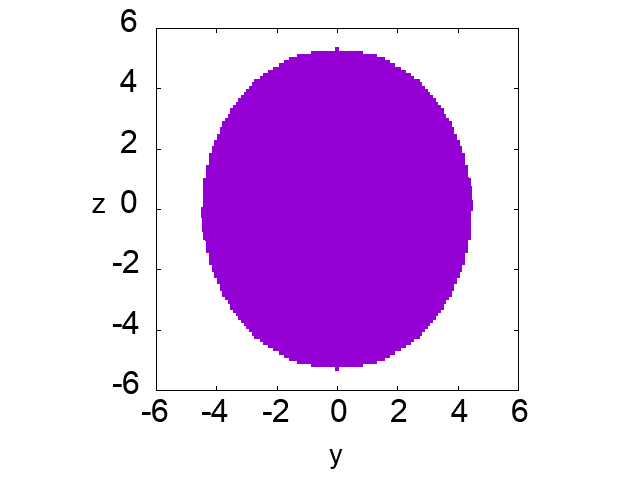
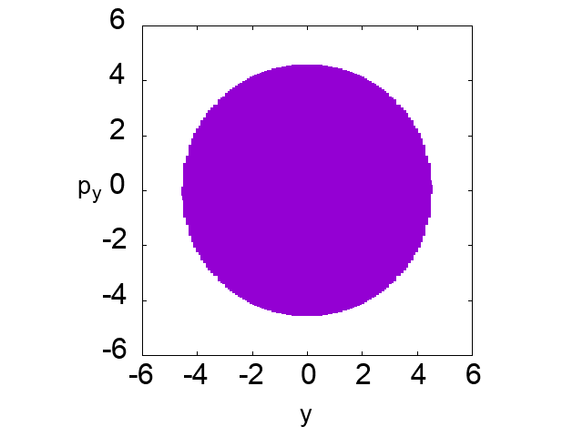
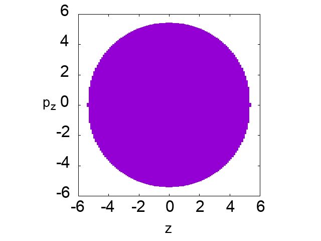
Figure 3: 2D projections of dividing surface that is constructed from the NHIM in $(y,z)$ (first panel), $(y,p_{y})$ (second panel) and $(z,p_{z})$ (third panel) subspaces of the phase space.

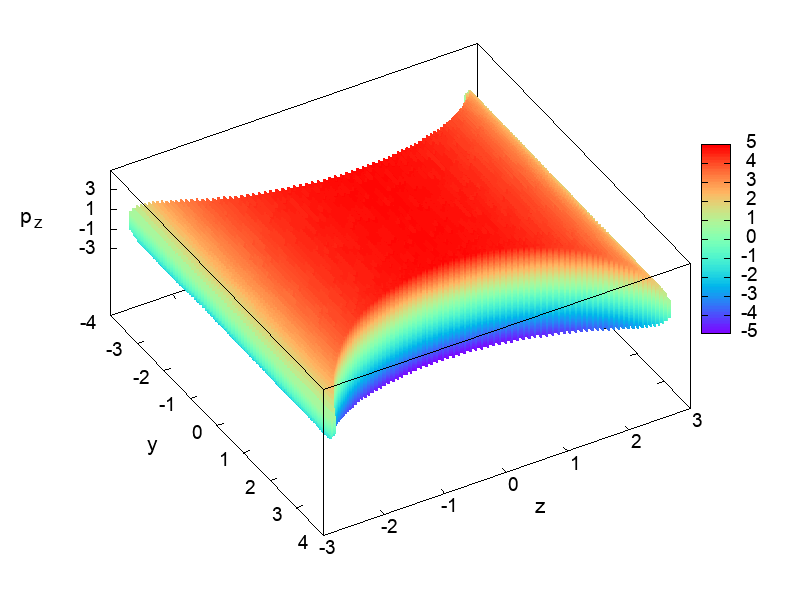
Figure 4: The 3D projection $(y,z,p_{z})$ of the dividing surface which is constructed from the periodic orbit PO1 with the associated torus to have r=Rmax. The color indicates the values of the third dimension. The same structure is encountered also in 3D projection $(z,p_{y},p_{z})$. The viewpoint is in spherical coordinates is $(30^{o},60^{o})$.

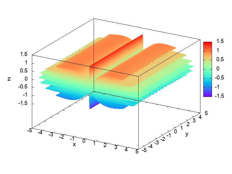
Figure 8: Trajectories in the 3D configuration space that have initial conditions on the dividing surfaces which is constructed from the periodic orbit PO1 with the associated torus to have r=Rmax/20. The color indicates the values of the third dimension. The viewpoint is in spherical coordinates is $(60^{o},30^{o})$.

5 The Algorithm for Hamiltonian systems with $n$ degrees of freedom

In the section 2 we described the difference between the two versions of our algorithm for the construction of dividing surfaces and when we use the one or other version. Now, we describe in detail the two versions of our algorithm in the case of Hamiltonian systems with $n$ degrees of freedom with a potential energy $V(x_{1},x_{2},...,x_{n})$:

$$T+V(x_{1},x_{2},...,x_{n})=E$$

where $T$ is the kinetic energy.

$$T=p_{x_{1}}^{2}/2m_{1}+p_{x_{2}}^{2}/2m_{2}+...+p_{x_{n}}^{2}/2m_{n}$$

where $p_{x_{1}},p_{x_{2}}...p_{x_{n}}$ are the momenta and $m_{1},m_{2},...m_{n}$ the corresponding masses.
When we apply the two versions of the algorithm to Hamiltonian systems with $n$ degrees of freedom we produce two algorithms, one algorithm for each version.

5.1 First Version

The first version of the algorithm is:

1. Locate an unstable periodic orbit PO for a fixed value of Energy $E$.

2. Project the PO into the configuration space and we consider a 2D subspace of the phase space in which the projection of the periodic orbit is a closed curve (for example in the $(x_{2},p_{x_{2}})$ space).

3. From the projection of the periodic orbit in the configuration space, we construct a torus that is generated by the Cartesian product of $n-1$ circles with small radius and the projection of the periodic orbit in a 2D subspace of the phase space (for example in the $(x_{2},p_{x_{2}})$ space). Actually topologically it is equivalent with the Cartesian product of $n$ circles $S^{1}\times S^{1}\times S^{1}\times...\times S^{1}$. This is a $n$-dimensional torus. This can be achieved through the construction of one circle around every point of the periodic orbit in a ($n+1$)D subspace of the phase space. For example we compute a circle (with a fixed radius r) in the plane $(x_{1},x_{2})$ around every point of the periodic orbit in the ($n+1$)D subspace $(x_{1},x_{2},...,x_{n},p_{x_{2}})$. Then we construct a new circle around every point of the previous structure in other 2D subspace of the ($n+1$)D subspace $(x_{1},...,x_{n},p_{x_{2}})$. This can be done computing a circle (with a fixed radius r) in the plane $(x_{2},x_{3})$. Then we continue adding circles until we will have added $n-1$ circles to the initial projection of the periodic orbit. The target of this step is to include all coordinates of the configuration space in this torus.

   $$x_{2,1,i,j1}=x_{2,0,i}+rcos(\theta_{j1})$$

   $$x_{1,1,i,j1}=x_{1,0,i}+rsin(\theta_{j1})$$

   $$x_{3,1,i,j1}=x_{3,0,i}$$

   $$...$$

   $$x_{n,1,i,j1}=x_{n,0,i}$$

   $$p_{x_{2},1,i,j1}=p_{x_{2},0,i}$$ (50)

   $$x_{2,2,i,j1,j2}=x_{2,1,i,j1}+rcos(\theta_{j2})$$

   $$x_{3,2,i,j1,j2}=x_{3,1,i,j1}+rsin(\theta_{j2})$$

   $$x_{1,2,i,j1,j2}=x_{1,1,i,j1}$$

   $$...$$

   $$x_{n,2,i,j1,j2}=x_{n,1,i,j1}$$

   $$p_{x_{2},2,i,j1,j2}=p_{x_{2},1,i,j1}$$

   $$...$$ (51)

   $$...$$

   $$x_{2,n-1,i,j1,j2,...,j(n-1)}=x_{2,n-2,i,j1,j2,...,j(n-2)}+rcos(\theta_{j(n-1)})$$

   $$x_{n,n-1,i,j1,j2...j(n-1)}=x_{n,n-2,i,j1,j2,...,j(n-2)}+rsin(\theta_{j(n-1)})$$

   $$x_{1,n-1,i,j1,j2,...j(n-1)}=x_{1,n-2,i,j1,j2,...,j(n-2)}$$

   $$...$$

   $$x_{n-1,n-1,i,j1,j2,...,j(n-1)}=x_{n-1,n-2,1,i,j1,j2,...,j(n-2)}$$

   $$p_{x_{2},n-1,i,j1,j2,...,j(n-1)}=p_{x_{2},n-2,i,j1,j2,...,j(n-2)}$$

   $(x_{1,0,i},x_{2,0,i},...,x_{n,0,i},p_{x_{2},0,i}),i=1,...N$ are the points of the periodic orbit in the $(n+1)$D subspace $(x_{1},x_{2},...,x_{n},p_{x_{2}})$. We have the angle $\theta_{j1}=j1\frac{2\pi}{n_{1}}$ with $j1=1,...,n_{1}$ for the first circle and $\theta_{j2}=j2\frac{2k\pi}{n_{1}}$ with $j2=1,...,n_{1}$ for the second circle and so on the $\theta_{j(n-1)}=j(n-1)\frac{2\pi}{n_{1}}$ with $j(n-1)=1,...,n_{1}$ for the $n-1$ circle that we need for the construction of the torus.

   $x_{1,1,i,j1},x_{1,1,i,j1},...,x_{n,1,i,j1},p_{x_{2},1,i,j1}$ with $i=1,...,N$ and $j1=1,...,n_{1}$ are the points of the torus that is constructed from the Cartesian product of projection of the periodic orbit in the 2D subspace $(x_{2},p_{x_{2}})$ and a circle in the $(x_{1},x_{2})$ space in the $(n+1)$D space $(x_{1},x_{2},...x_{n},p_{x_{2}})$. $x_{2,2,i,j1,j2},x_{1,2,i,j1,j2},...x_{n,2,i,j1,j2},p_{x_{2},2,i,j1,j2}$ with $i=1,...,N$, $j1=1,...,n_{1}$ and $j2=1,...,n_{1}$ are the points of the torus that is constructed from the Cartesian product of the projection of the periodic orbit in the 2D subspace $(x_{2},p_{x_{2}})$, and other 2 circles in the ($n+1$)D space $(x_{1},x_{2},...,x_{n},p_{x_{2}})$. And so on $x_{1,n-1,i,j1,j2,...j(n-1)},x_{2,n-1,i,j1,j2,...j(n-1)},...x_{n,n-1,i,j1,j2,..j(n-1)},p_{x_{2},n-1,i,j1,j2,...j(n-1)}$ with $i=1,...,N$ and $j1,j2,....j(n-1)=1,...,n_{1}$ are the points of the torus that is constructed from the Cartesian product of the projection of the periodic orbit in the 2D subspace $(x_{2},p_{x_{2}})$, and other $n-1$ circles in the ($n+1$)D space $(x_{1},x_{2},...,x_{n},p_{x_{2}})$.

4. For each point $x_{1,n-1,i,j1,j2,...j(n-1)},x_{2,n-1,i,j1,j2,...j(n-1)},...x_{n,n-1,i,j1,j2,..j(n-1)},p_{x_{2},n-1,i,j1,j2,...j(n-1)}$ with $i=1,...,N$ and $j1,j2,....j(n-1)=1,...,n_{1}$ on this torus we must calculate the $p_{x_{1},n-1,i,j1,j2,,...j(n-1)}^{max}$ and $p_{x_{1},n-1,i,j1,j2,,...j(n-1)}^{min}$ by solving the following equation for a fixed value of energy (Hamiltonian) E with $p_{x_{3}}=...=p_{x_{n}}=0$:

   $$V(x_{1,n-1,i,j1,j2,...j(n-1)},x_{2,n-1,i,j1,j2,...j(n-1)},...x_{n,n-1,i,j1,j2,..j(n-1)})+$$

   $$\frac{p_{x_{1},n-1,i,j1,j2,...j(n-1)}^{2}}{2m_{1}}+\frac{p_{x_{2},n-1,i,j1,j2,...j(n-1)}^{2}}{2m_{2}}=E$$

   and we find the maximum and minimum values
   $p_{x_{1},n-1,i,j1,j2,...j(n-1)}^{max}$ and $p_{x_{1},n-1,i,j1,j2,...j(n-1)}^{min}$. We choose points $p_{x_{1},n-1,i,j1,j2,...j(n-1)}$ with $j1,j2...j(n-1)=1,...,n_{1}$ in the interval $p_{x_{1},n-1,i,j1,j2,...j(n-1)}^{min}\leq p_{x_{1},n-1,i,j1,j2,...j(n-1)}\leq p_{x_{1},n-1,i,j1,j2,...j(n-1)}^{max}$. These points can be uniformly distributed in this interval. We will repeat the same procedure to compute the values $p_{x_{3},n-1,i,j1,j2,...j(n-1)},...,p_{x_{n-1},n-1,i,j1,j2,...j(n-1)}$. In general for $n_{2}\leq n-1$ for each point $x_{1,n-1,i,j1,j2,...j(n-1)},x_{2,n-1,i,j1,j2,...j(n-1)},...x_{n,n-1,i,j1,j2,..j(n-1)},p_{x_{1},n-1,i,j1,j2,...j(n-1)},...\\ p_{x_{n_{2}-1},n-1,i,j1,j2,...j(n-1)}$ with $i=1,...,N$ and $j1,j2,....j(n-1)=1,...,n_{1}$ we must calculate the $p_{x_{n_{2}},n-1,i,j1,j2,,...j(n-1)}^{max}$ and $p_{x_{n_{2}},n-1,i,j1,j2,,...j(n-1)}^{min}$ by solving the following equation for a fixed value of energy (Hamiltonian) E with $p_{x_{n_{2}+1}}=...=p_{x_{n}}=0$:

   $$V(x_{1,n-1,i,j1,j2,...j(n-1)},x_{2,n-1,i,j1,j2,...j(n-1)},...x_{n,n-1,i,j1,j2,..j(n-1)})+$$

   $$\frac{p_{x_{1},n-1,i,j1,j2,...j(n-1)}^{2}}{2m_{1}}+...+\frac{p_{x_{n_{2}},n-1,i,j1,j2,...j(n-1)}^{2}}{2m_{n_{2}}}=E$$

   and we find the maximum and minimum values $p_{x_{n_{2}},n-1,i,j1,j2,...j(n-1)}^{max}$ and $p_{x_{n_{2}},n-1,i,j1,j2,...j(n-1)}^{min}$. We choose points $p_{x_{n_{2}},n-1,i,j1,j2,...j(n-1)}$ with $j1,j2,j(n-1)=1,...,n_{1}$ in the interval $p_{x_{n_{2}},n-1,i,j1,j2,...j(n-1)}^{min}\leq p_{x_{n_{2}},n-1,i,j1,j2,...j(n-1)}\leq p_{x_{n_{2}},n-1,i,j1,j2,...j(n-1)}^{max}$. These points can be uniformly distributed in this interval.

   Then we obtain the value $p_{x_{n},n-1,i,j1,j2,...j(n-1)}$ from the Hamiltonian:

   $$V(x_{1,n-1,i,j1,j2,...j(n-1)},x_{2,n-1,i,j1,j2,...j(n-1)},...x_{n,n-1,i,j1,j2,..j(n-1)})+$$

   $$\frac{p_{x_{1},n-1,i,j1,j2,...j(n-1)}^{2}}{2m_{1}}+...+\frac{p_{x_{n},n-1,i,j1,j2,...j(n-1)}^{2}}{2m_{n}}=E$$

Dimensionality and Topology: This algorithm constructs a torus as the product of the closed curve that represents the projection of the periodic orbit (1D object) in a 2D subspace with $n-1$ circles in the ($n+1$)D subspace of the energy manifold. This torus is a n-dimensional torus. Then we sample the $n-2$ variables ($n-2$ momenta) in the interval between their maximum and minimum value. Actually we create $n-2$ additional segments and we increase the dimensionality of the initial torus, from n to $2n-2$ dimensions, which is embedded in the $2n-1$ energy surface. Then we obtain the value of the last momentum from the Hamiltonian of the system.

5.2 Second Version

The second version is:

1. Locate an unstable periodic orbit PO for a fixed value of Energy $E$.

2. Project the PO into the configuration space and we consider a 2D subspace of the configuration space in which the projection of the periodic orbit is a closed curve (for example in the $(x_{1},x_{2})$ space).

3. From the projection of the periodic orbit in the configuration space, we construct a torus that is generated by the Cartesian product of $n-2$ circles with small radius and the projection of the periodic orbit in a 2D subspace of the configuration space (for example in the $(x_{1},x_{2})$ space). Actually topologically it is equivalent with the Cartesian product of $n-1$ circles $S^{1}\times S^{1}\times S^{1}\times...\times S^{1}$. This is a $n-1$-dimensional torus. This can be achieved through the construction of one circle around every point of the periodic orbit in a $n$D subspace of the phase space (configuration space). For example we compute a circle (with a fixed radius r) in the plane $(x_{2},x_{3})$ around every point of the periodic orbit in the $n$D configuration space $(x_{1},x_{2},...,x_{n})$. Then we construct a new circle around every point of the previous structure in other 2D subspace of the $n$D configuration space $(x_{1},...,x_{n})$. This can be done computing a circle (with a fixed radius r) in the plane $(x_{2},x_{4})$. Then we continue adding circles until we will have added $n-2$ circles to the initial projection of the periodic orbit. The target of this step is to include all coordinates of the configuration space in this torus.

   $$x_{2,1,i,j1}=x_{2,0,i}+rcos(\theta_{j1})$$

   $$x_{3,1,i,j1}=x_{3,0,i}+rsin(\theta_{j1})$$

   $$x_{1,1,i,j1}=x_{1,0,i}$$

   $$x_{4,1,i,j1}=x_{4,0,i}$$

   $$...$$

   $$x_{n,1,i,j1}=x_{n,0,i}$$

   $$x_{2,2,i,j1,j2}=x_{2,1,i,j1}+rcos(\theta_{j2})$$

   $$x_{4,2,i,j1,j2}=x_{4,1,i,j1}+rsin(\theta_{j2})$$

   $$x_{1,2,i,j1,j2}=x_{1,1,i,j1}$$

   $$x_{3,2,i,j1,j2}=x_{3,1,i,j1}$$

   $$...$$

   $$x_{n,2,i,j1,j2}=x_{n,1,i,j1}$$

   $$...$$ (57)

   $$...$$

   $$x_{2,n-2,i,j1,j2,...,j(n-2)}=x_{2,n-3,i,j1,j2,...,j(n-3)}+rcos(\theta_{j(n-2)})$$

   $$x_{n,n-2,i,j1,j2...j(n-2)}=x_{n,n-3,i,j1,j2,...,j(n-3)}+rsin(\theta_{j(n-2)})$$

   $$x_{1,n-2,i,j1,j2,...j(n-2)}=x_{1,n-3,i,j1,j2,...,j(n-3)}$$

   $$...$$

   $$x_{n-1,n-2,i,j1,j2,...,j(n-2)}=x_{n-1,n-3,1,i,j1,j2,...,j(n-3)}$$

   $(x_{1,0,i},x_{2,0,i},...,x_{n,0,i}),i=1,...N$ are the points of the periodic orbit in the $n$D configuration space $(x_{1},x_{2},...,x_{n})$. We have the angle $\theta_{j1}=j1\frac{2\pi}{n_{1}}$ with $j1=1,...,n_{1}$ for the first circle and $\theta_{j2}=j2\frac{2k\pi}{n_{1}}$ with $j2=1,...,n_{1}$ for the second circle and so on the $\theta_{j(n-2)}=j(n-2)\frac{2\pi}{n_{1}}$ with $j(n-2)=1,...,n_{1}$ for the $n-2$ circle that we need for the construction of the torus.

   $x_{1,1,i,j1},x_{2,1,i,j1},...,x_{n,1,i,j1}$ with $i=1,...,N$ and $j1=1,...,n_{1}$ are the points of the torus that is constructed from the Cartesian product of the projection of the periodic orbit in the 2D subspace $(x_{1},x_{2})$ and a circle in the $n$D space $(x_{1},x_{2},...x_{n})$. $x_{1,2,i,j1,j2},x_{2,2,i,j1,j2},...x_{n,2,i,j1,j2}$ with $i=1,...,N$, $j1=1,...,n_{1}$ and $j2=1,...,n_{1}$ are the points of the torus that is constructed from the Cartesian product of the projection of the periodic orbit in the 2D subspace $(x_{1},x_{2})$, and other 2 circles in the $n$D space $(x_{1},x_{2},...,x_{n})$. And so on $x_{1,n-2,i,j1,j2,...j(n-2)},x_{2,n-2,i,j1,j2,...j(n-2)},...x_{n,n-2,i,j1,j2,..j(n-2)}$ with $i=1,...,N$ and $j1,j2,....j(n-2)=1,...,n_{1}$ are the points of the torus that is constructed from the Cartesian product of the projection of the periodic orbit in the 2D subspace $(x_{1},x_{2})$, and other $n-2$ circles in the $n$D space $(x_{1},x_{2},...,x_{n})$.

4. For each point $x_{1,n-2,i,j1,j2,...j(n-2)},x_{2,n-2,i,j1,j2,...j(n-2)},...x_{n,n-2,i,j1,j2,..j(n-2)}$ with $i=1,...,N$ and $j1,j2,....j(n-2)=1,...,n_{1}$ on this torus we must calculate the $p_{x_{1},n-2,i,j1,j2,,...j(n-2)}^{max}$ and $p_{x_{1},n-2,i,j1,j2,,...j(n-2)}^{min}$ by solving the following equation for a fixed value of energy (Hamiltonian) E with $p_{x_{2}}=p_{x_{3}}=...=p_{x_{n}}=0$:

   $$V(x_{1,n-2,i,j1,j2,...j(n-2)},x_{2,n-2,i,j1,j2,...j(n-2)},...x_{n,n-2,i,j1,j2,..j(n-2)})+$$

   $$\frac{p_{x_{1},n-2,i,j1,j2,...j(n-2)}^{2}}{2m_{1}}=E$$

   and we find the maximum and minimum values
   $p_{x_{1},n-2,i,j1,j2,...j(n-2)}^{max}$ and $p_{x_{1},n-2,i,j1,j2,...j(n-2)}^{min}$. We choose points $p_{x_{1},n-2,i,j1,j2,...j(n-2)}$ with $j1,j2...j(n-2)=1,...,n_{1}$ in the interval $p_{x_{1},n-2,i,j1,j2,...j(n-2)}^{min}\leq p_{x_{1},n-2,i,j1,j2,...j(n-2)}\leq p_{x_{1},n-2,i,j1,j2,...j(n-2)}^{max}$. These points can be uniformly distributed in this interval. We will repeat the same procedure to compute the values $p_{x_{2},n-2,i,j1,j2,...j(n-2)},...,p_{x_{n-1},n-2,i,j1,j2,...j(n-2)}$. In general for $n_{2}\leq n-1$ for each point $x_{1,n-2,i,j1,j2,...j(n-2)},x_{2,n-2,i,j1,j2,...j(n-2)},...x_{n,n-2,i,j1,j2,..j(n-2)},p_{x_{1},n-2,i,j1,j2,...j(n-2)},...\\ p_{x_{n_{2}-1},n-2,i,j1,j2,...j(n-2)}$ with $i=1,...,N$ and $j1,j2,....j(n-2)=1,...,n_{1}$ we must calculate the $p_{x_{n_{2}},n-2,i,j1,j2,,...j(n-2)}^{max}$ and $p_{x_{n_{2}},n-2,i,j1,j2,,...j(n-2)}^{min}$ by solving the following equation for a fixed value of energy (Hamiltonian) $E$ with $p_{x_{n_{2}+1}}=...=p_{x_{n}}=0$:

   $$V(x_{1,n-2,i,j1,j2,...j(n-2)},x_{2,n-2,i,j1,j2,...j(n-2)},...x_{n,n-2,i,j1,j2,..j(n-2)})+$$

   $$\frac{p_{x_{1},n-2,i,j1,j2,...j(n-2)}^{2}}{2m_{1}}+...+\frac{p_{x_{n_{2}},n-2,i,j1,j2,...j(n-2)}^{2}}{2m_{n_{2}}}=E$$

   and we find the maximum and minimum values $p_{x_{n_{2}},n-2,i,j1,j2,...j(n-2)}^{max}$ and $p_{x_{n_{2}},n-2,i,j1,j2,...j(n-2)}^{min}$. We choose points $p_{x_{n_{2}},n-2,i,j1,j2,...j(n-2)}$ with $j1,j2,j(n-2)=1,...,n_{1}$ in the interval $p_{x_{n_{2}},n-2,i,j1,j2,...j(n-2)}^{min}\leq p_{x_{n_{2}},n-2,i,j1,j2,...j(n-2)}\leq p_{x_{n_{2}},n-2,i,j1,j2,...j(n-2)}^{max}$. These points can be uniformly distributed in this interval.

   Then we obtain the value $p_{x_{n},n-2,i,j1,j2,...j(n-2)}$ from the Hamiltonian:

   $$V(x_{1,n-2,i,j1,j2,...j(n-2)},x_{2,n-2,i,j1,j2,...j(n-2)},...x_{n,n-2,i,j1,j2,..j(n-2)})+$$

   $$\frac{p_{x_{1},n-2,i,j1,j2,...j(n-2)}^{2}}{2m_{1}}+...+\frac{p_{x_{n},n-2,i,j1,j2,...j(n-2)}^{2}}{2m_{n}}=E$$

Dimensionality and Topology: This algorithm constructs a torus as the product of the closed curve that represents the projection of the periodic orbit (1D object) in a 2D subspace of the configuration space with $n-2$ circles in the $n$D configuration space . This torus is a $n-1$-dimensional torus. Then we sample the $n-1$ variables ($n-1$ momenta) in the interval between their maximum and minimum value. Actually we create $n-1$ additional segments and we increase the dimensionality of the initial torus, from $n-1$ to $2n-2$ dimensions, which is embedded in the $2n-1$ energy surface. Then we obtain the value of the last momentum from the Hamiltonian of the system.

6 Conclusions

We generalized the notion of the periodic orbit dividing surface construction to Hamiltonian systems with $n$ degrees of freedom. This is very important because until now this surface was computed only in Hamiltonian systems with two degrees of freedom though the classical method of Pechukas [1981] and Pollak [1985]. For Hamiltonian systems with three or more degrees of freedom, the dividing surfaces could be computed using as a starting point the Normally Hyperbolic Invariant Manifold (NHIM- see Wiggins [2016], Wiggins [1994]) and not periodic orbits. In many systems this is very difficult and we need the Normal form theory to compute this structure. In this method we use the periodic orbit as a starting point and we construct a torus as a Cartesian product of $n-1$ circle or $n-2$ circles and a 2D projection of the periodic orbit avoiding the difficult computation of the NHIM. We compare the dividing surfaces from the periodic orbits with the dividing surface from the NHIM in a simple Normal Form quadratic Hamiltonian system with two and three degrees of freedom. From all these we have the following remarks:

1. Our algorithm for the construction of the periodic orbit dividing surfaces is valid in the cases in which the periodic orbits are closed curves in a 2D subspace of the configuration space or a 2D subspace of the extended configuration space (a space that consists of the configuration space plus 1D space that corresponds to one of the momenta).

2. We have two versions of our algorithm for the construction of the dividing surfaces from periodic orbits. The choice of one of these versions depends from the fact if the periodic orbit is closed curve in a 2D subspace of the configuration space or not.

3. In Hamiltonian systems with two degrees of freedom the second version of our algorithm for the construction of dividing surfaces coincides with the classical method of Pechukas [1981] and Pollak [1985].

4. In Hamiltonian systems with three degrees of freedom, the periodic orbit dividing surfaces have the topology of a hyperbolic torus.

5. The periodic orbit dividing surfaces that are constructed from our algorithm are subsets of the dividing surfaces that are constructed from the NHIM.

6. According to the position of the periodic orbits in the phase space the associated dividing surfaces, that are constructed from our algorithm, give us the trajectory behaviour for different regions of the configuration space. For example in our case (a Normal form Hamiltonian system with three degrees of freedom) the PO1 dividing surface give us more information for the trajectories in the y-direction and PO2 dividing surface give us more information in the z-direction.

7. The radius of the circles that are needed for the construction of the periodic orbit dividing surfaces, through our algorithm, is crucial for the efficiency of the algorithm and the size of the dividing surfaces.

AcknowledgmentsWe acknowledge the support of EPSRC Grant No. EP/P021123/1 and ONR Grant No. N00014-01-1-0769.

References

• Ezra & Wiggins [2018] Ezra, G.Β S. & Wiggins, S. [2018] β€œSampling phase space dividing surfaces constructed from normally hyperbolic invariant manifolds (nhims),” The Journal of Physical Chemistry A 122, 8354–8362.
• Komatsuzaki & Berry [2003] Komatsuzaki, T. & Berry, R.Β S. [2003] β€œChemical reaction dynamics: Many-body chaos and regularity,” Adv. Chem. Phys. , 79–152.
• Pechukas [1981] Pechukas, P. [1981] β€œTransition state theory,” Annual Review of Physical Chemistry 32, 159–177.
• Pechukas & McLafferty [1973] Pechukas, P. & McLafferty, F.Β J. [1973] β€œOn transition-state theory and the classical mechanics of collinear collisions,” The Journal of Chemical Physics 58, 1622–1625.
• Pechukas & Pollak [1977] Pechukas, P. & Pollak, E. [1977] β€œTrapped trajectories at the boundary of reactivity bands in molecular collisions,” The Journal of Chemical Physics 67, 5976–5977.
• Pechukas & Pollak [1979] Pechukas, P. & Pollak, E. [1979] β€œClassical transition state theory is exact if the transition state is unique,” The Journal of Chemical Physics 71, 2062–2068.
• Pollak [1985] Pollak, E. [1985] β€œPeriodic orbits and the theory of reactive scattering,” Theory of Chemical Reaction Dynamics 3, 123.
• Pollak & Pechukas [1978] Pollak, E. & Pechukas, P. [1978] β€œTransition states, trapped trajectories, and classical bound states embedded in the continuum,” The Journal of Chemical Physics 69, 1218–1226.
• Toda [2003] Toda, M. [2003] β€œDynamics of chemical reactions and chaos,” Adv. Chem. Phys. 123, 153–198.
• Uzer etΒ al. [2002] Uzer, T., JaffΓ©, C., PalaciΓ‘n, J., Yanguas, P. & Wiggins, S. [2002] β€œThe geometry of reaction dynamics,” Nonlinearity 15, 957–992.
• Waalkens etΒ al. [2007] Waalkens, H., Schubert, R. & Wiggins, S. [2007] β€œWigner’s dynamical transition state theory in phase space: classical and quantum,” Nonlinearity 21, R1–R118.
• Waalkens & Wiggins [2010] Waalkens, H. & Wiggins, S. [2010] β€œGeometrical models of the phase space structures governing reaction dynamics,” Regular and Chaotic Dynamics 15, 1–39.
• Wiggins [1994] Wiggins, S. [1994] Normally hyperbolic invariant manifolds in dynamical systems (springer verlag).
• Wiggins [2016] Wiggins, S. [2016] β€œThe role of normally hyperbolic invariant manifolds (nhims) in the context of the phase space setting for chemical reaction dynamics,” Regular and Chaotic Dynamics 21, 621–638.
• Wiggins etΒ al. [2001] Wiggins, S., Wiesenfeld, L., JaffΓ©, C. & Uzer, T. [2001] β€œImpenetrable barriers in phase-space,” Physical Review Letters 86, 5478–5481.
• Wigner [1938] Wigner, E. [1938] β€œThe transition state method,” Transactions of the Faraday Society 34, 29–41.