Cosmological evolution in $f(T,B)$ gravity

Abstract

For the fourth-order teleparallel $f\left(T,B\right)$ theory of gravity, we investigate the cosmological evolution for the universe in the case of a spatially flat Friedmann–Lemaître–Robertson–Walker background space. We focus on the case for which $f\left(T,B\right)$ is separable, that is, $f\left(T,B\right)_{,TB}=0$ and $f\left(T,B\right)$ is a nonlinear function on the scalars $T$ and $B$. For this fourth-order theory we use a Lagrange multiplier to introduce a scalar field function which attributes the higher-order derivatives. In order to perform the analysis of the dynamics we use dimensionless variables which allow the Hubble function to change sign. The stationary points of the dynamical system are investigated both in the finite and infinite regimes. The physical properties of the asymptotic solutions and their stability characteristics are discussed.

I Introduction

Modified and extended theories of gravity have drawn the attention of cosmologists in recent years because they provide a systematic and geometric approach for the explanation of the cosmological observations sp1 ; sp2 ; sp3 ; fg5 ; fg6 ; fg7 ; fg10 ; fg10a ; fg10b . In the family of modified theories of gravity known as $f$-theories the gravitational Action Integral is defined to be a function $f$ of specific geometric invariants fg2 ; fg3 ; fg4 ; fg11 ; fg12 ; fg14 ; fg15 ; fg16 ; fg17 ; fg18 ; fg19 ; fg20 . The simplest $f$-theory is the $f\left(R\right)$ gravity Buda in which the Einstein-Hilbert Action, with or without the cosmological constant, is recovered when $f\left(R\right)$ is a linear function. The main characteristic of $f$-theories is that the new modified field equations provide geometrodynamical components which drive the dynamics in order to explain the cosmological evolution, while General Relativity should be recovered.

In this study we are interested in an extended higher-order teleparallel $f$-theory known as $f\left(T,B\right)$ theory bahamonde , where $T$ is the scalar function of the Weitzenböck connection and $B$ is the boundary term which is the difference between $T$ and Ricci scalar $R~{}$myr11 . The essential variables of teleparallel theory are the vierbein fields, and scalar function $T$ is defined by first derivatives. Consequently, a linear $f\left(T,B\right)=f_{1}T+f_{2}B$ theory is a second-order theory. It describes the teleparallel equivalence of General Relativity ein28 ; Hayashi79 . Furthermore, any $f\left(T,B\right)=F\left(T\right)+f_{2}B$ is also a second-order theory known as $F\left(T\right)$ theory Ferraro . In the following we consider that $f\left(T,B\right)$ is separable, i.e.  $f\left(T,B\right)_{,TB}=0$ and $f\left(T,B\right)$ is a nonlinear function of $T$ and $B$, i.e. $f_{,TT}\neq 0$ and $f_{,BB}\neq 0$. Hence, the resulting theory is a fourth-order theory because $B$ includes second derivatives of the vierbein fields.

In ftb01 the authors investigated the gravitomagnetism characteristic phenomena in the weak field in $f\left(T,B\right)$ theory. Moreover, cosmological bouncing solutions were studied in ftb02 while the cosmological perturbations of the theory were investigated in ftb02a . The linear function $F$ in the scalar function $T~{}$ was the subject of study in anprd where a scalar field description was used in order to write the field equations as second-order differential equations. The theory admits a minisuperspace description which was applied to study the quantization and the Wheeler-DeWitt equation an11 . Some other studies of $f\left(T,B\right)$ theory which we discuss in the following sections are anjcap ; angrg ; cel1 ; cel2 . The plan of the paper is as follows.

In Section II, we present the cosmological model of our consideration. We consider $f\left(T,B\right)$ teleparallel theory where $f\left(T,B\right)=F\left(T\right)+\beta\left(B\right)$ and $F\left(T\right),~{}\beta\left(B\right)$ are nonlinear functions.  In addition, for the background space, we assume a spatially flat Friedmann–Lemaître–Robertson–Walker (FLRW) spacetime. For this cosmological model the field equations are of fourth-order in the scale factor. However, we define a new scalar field which attributes the additional degrees of freedom such that to write the field equations as second-order equations by increasing the number of dependent variables. Hence, the dependent variables are the scalar factor and the new scalar field. In Section III we present the main results of our analysis. We perform a detailed analysis of the dynamics for the cosmological field equations by using dimensionless variables. Because of the geometric terms in the field equations which correspond to the higher-order derivatives, we observe that the Hubble function can change sign during the cosmological evolution. Hence, a new set of variables, different from those of the Hubble normalization, are defined which allow the Hubble function to be continuous in whole range of values. We investigate the stationary points and their stability properties for the field equations in the new variables. Every stationary point corresponds to a specific epoch in the cosmological history and provides us with important information about the cosmological evolution and the viability of the theory. The stationary points are studied in the finite and the infinite regimes. Finally, in Section IV we summarize our results and we draw our conclusions.

II $f\left(T,B\right)$ cosmology

In this work we consider the fourth-order generalized teleparallel theory of gravity known as $f\left(T,B\right)$ theory. Contrary to General Relativity, in teleparallel theories the dynamical variables are the vierbein fields. The later form an orthonormal basis for the tangent space at each point, $x^{\mu}$, of the manifold,$~{}g(e_{i},e_{j})=\mathbf{e}_{i}\cdot\mathbf{e}_{i}=\eta_{ij}$, where $\eta_{ij}~{}$is the four-dimensional Minkowski spacetime. The equivalent form in the coordinate system

$$g_{\mu\nu}(x)=\eta_{ij}h_{\mu}^{i}(x)h_{\nu}^{j}(x)~{},~{}e_{i}=h_{i}^{\mu}\left(x\right)\partial_{i}.$$ (1)

By definition, the fundamental connection in teleparallel theories is the Weitzenböck connection $\hat{\Gamma}^{\lambda}{}_{\mu\nu}=h_{a}^{\lambda}\partial_{\mu}h_{\nu}^{a}$, from where we can define the nonnull torsion tensor, ftt0 ; ftt1

$$T_{\mu\nu}^{\beta}=\hat{\Gamma}_{\nu\mu}^{\beta}-\hat{\Gamma}_{\mu\nu}^{\beta}=h_{i}^{\beta}(\partial_{\mu}h_{\nu}^{i}-\partial_{\ qu}h_{\mu}^{i}),$$ (2)

with scalar

$$T={S_{\beta}}^{\mu\nu}{T^{\beta}}_{\mu\nu},~{}$$

in which ${S_{\beta}}^{\mu\nu}~{}$is defined as ${S_{\beta}}^{\mu\nu}=\frac{1}{2}({K^{\mu\nu}}_{\beta}+\delta_{\beta}^{\mu}{T^{\theta\nu}}_{\theta}-\delta_{\beta}^{\nu}{T^{\theta\mu}}_{\theta}).~{}T$ is the scalar function which is used for the definition of the gravitational Action Integral. The quantity ${K^{\mu\nu}}_{\beta}$ is the contorsion tensor and equals the difference between the Levi-Civita connections in the holonomic and the nonholonomic frame. ${K^{\mu\nu}}_{\beta}~{}$is defined as ${K^{\mu\nu}}_{\beta}=-\frac{1}{2}({T^{\mu\nu}}_{\beta}-{T^{\nu\mu}}_{\beta}-{T_{\beta}}^{\mu\nu}).$

In $f\left(T,B\right)$ gravity the gravitational Action Integral is a function $f$ of the scalar $T$ and of the boundary term $B$ which is the boundary term $B=2e_{\nu}^{-1}\partial_{\nu}\left(eT_{\rho}^{~{}\rho\nu}\right)$, that is, bahamonde

$$S\equiv\frac{1}{16\pi G}\int d^{4}xef\left(T,B\right),$$ (3)

in which $e=\det(e_{\mu}^{i})=\sqrt{-g}.~{}$Because $B=R+T$, where$~{}R$ is the Ricci scalar, the Action Integral (3) is equivalent to anprd

$$S\equiv\frac{1}{16\pi G}\int d^{4}xe\bar{f}\left(T,R\right),~{}\text{or~{}}S\equiv\frac{1}{16\pi G}\int d^{4}xe\hat{f}\left(R,B\right)~{},$$

in which $f\left(T,B\right)=\bar{f}\left(T,R\right)$ and $f\left(T,B\right)=\hat{f}\left(R,B\right)$.

The field equations follow from the variation of (3) with respect to the vierbein fields, bahamonde

$$0 =\frac{1}{2}eh_{a}^{\lambda}\left(f_{,B}\right)^{;\mu\nu}g_{\mu\nu}-\frac{1}{2}eh_{a}^{\sigma}\left(f_{,B}\right)_{;\sigma}^{~{}~{}~{};\lambda}+\frac{1}{4}e\left(Bf_{,B}-\frac{1}{4}f\right)h_{a}^{\lambda}\,+(eS_{a}{}^{\mu\lambda})_{,\mu}f_{,T}$$

$$~{}\ ~{}+e\left((f_{,B})_{,\mu}+(f_{,T})_{,\mu}\right)S_{a}{}^{\mu\lambda}~{}-ef_{,T}T^{\sigma}{}_{\mu a}S_{\sigma}{}^{\lambda\mu},$$ (4)

where “;”    denotes the covariant derivative. The field equations (4) for a linear function $f\left(T,B\right)=f_{1}T+f_{2}B$ reduce to that of Einstein teleparallel theory of gravity, which is equivalent with General Relativity, while, if it is linear, to $B$, i.e. $f\left(T,B\right)=F\left(T\right)+f_{2}B$, the second-order $F\left(T\right)$ teleparallel gravity is recovered. In addition, when $f\left(T,B\right)=f\left(T-B\right),$ i.e. $f\left(T,B\right)=f\left(R\right)$, the field equations (4) are those of the fourth-order theory known as $f\left(R\right)$ theory.

With the use of the Einstein tensor, $G_{a}^{\lambda}$, the field equations (4) can be written in the equivalent form

$$eG_{a}^{\lambda}=G_{eff}\left(\mathcal{T}_{a}^{\left(T\right)}{}^{\lambda}+\mathcal{T}_{a}^{\left(B\right)}{}{}^{\lambda}\right),$$ (5)

in which $G_{eff}=\frac{4\pi G}{f_{,T}}$ is the effective varying gravitational constant and $\mathcal{T}_{a}^{\left(T\right)}{}^{\lambda},$ and $\mathcal{T}_{a}^{\left(B\right)}{}{}^{\lambda}$ are the effective energy momentum tensors anprd

$$4\pi Ge\mathcal{T}_{a}^{\left(T\right)}{}^{\lambda}=-\left[\frac{1}{4}\left(Tf_{,T}-f\right)eh_{a}^{\lambda}+e(f_{,T})_{,\mu}S_{a}{}^{\mu\lambda}\right],$$ (6)

$$4\pi Ge\mathcal{T}_{a}^{\left(B\right)}{}^{\lambda}=-\left[e(f_{,B})_{,\mu}S_{a}{}^{\mu\lambda}-\frac{1}{2}e\left(h_{a}^{\sigma}\left(f_{,B}\right)_{;\sigma}^{~{}~{}~{};\lambda}-h_{a}^{\lambda}\left(f_{,B}\right)^{;\mu\nu}g_{\mu\nu}\right)+\frac{1}{4}eBf_{,B}h_{a}^{\lambda}\right].$$ (7)

In this work we are interested in the case for which $f\left(T,B\right)=F\left(T\right)+\beta\left(B\right)$. In such consideration, the effective energy momentum tensors are written as anprd

$$4\pi Ge\mathcal{T}_{a}^{\left(T\right)}{}^{\lambda}=-\left[\frac{1}{4}\left(TF_{,T}-F\right)eh_{a}^{\lambda}+e(F_{,TT})T_{,\mu}S_{a}{}^{\mu\lambda}\right]$$ (8)

$$4\pi Ge\mathcal{T}_{a}^{\left(B\right)}{}^{\lambda} =-e(\beta\left(B\right)_{,BB})B_{;\mu}S_{a}{}^{\mu\lambda}-\frac{1}{4}e\left(B\beta\left(B\right)_{,B}-\beta\left(B\right)\right)h_{a}^{\lambda}$$ (9)

$$+\frac{1}{2}e\left(h_{a}^{\sigma}\left(\beta\left(B\right)_{,B}\right)_{;\sigma}^{~{}~{}~{};\lambda}-h_{a}^{\lambda}\left(\beta\left(B\right)_{,B}\right)^{;\mu\nu}g_{\mu\nu}\right)$$

while the varying gravitational constant is $\frac{G_{eff}}{4\pi G}=\left(F_{,T}\right)^{-1}.~{}$ In such a case, in $\frac{\partial\mathcal{T}_{a}^{\left(T\right)}{}^{\lambda}}{\partial B}=0$ and ${}\frac{\partial\mathcal{T}_{a}^{\left(B\right)}{}^{\lambda}}{\partial T}=0,$ which we can say that there is no interaction in the Action Integral between the two effective fluids.

Moreover, in such a case the energy-momentum tensor which includes the higher-order derivatives of the $f\left(T,B\right)$ theory can be written in an equivalent form by using a scalar field. Indeed, if we define $\phi=\beta\left(B\right)_{,B}$, then (9) is simplified as anjcap

$$4\pi Ge\mathcal{T}_{a}^{\left(B\right)}{}^{\lambda}=-\left[e\phi_{;\mu}S_{a}{}^{\mu\lambda}-\frac{1}{2}e\left(h_{a}^{\sigma}\left(\phi\right)_{;\sigma}^{~{}~{}~{};\lambda}-h_{a}^{\lambda}\left(\phi\right)^{;\mu\nu}g_{\mu\nu}\right)-\frac{1}{4}eV\left(\phi\right)h_{a}^{\lambda}\right],$$ (10)

where $V\left(\phi\right)=\left(\beta\left(B\right)-B\beta\left(B\right)_{,B}\right)$.

This is not a canonical scalar field and the theory does not belong to the scalar tensor theories. However, there is a direct relation with the teleparallel dark energy models cd1 under the action of conformal transformations ww1 .

II.1 FLRW background space

According to the cosmological principle for the background space we consider a spatially flat FLRW spacetime described by the scale factor $a\left(t\right)$ with line element

$$ds^{2}=N^{2}\left(t\right)dt^{2}-a^{2}\left(t\right)\left(dx^{2}+dy^{2}+dz^{2}\right),$$ (11)

where $N\left(t\right)$ is the lapse function. For the vierbein we consider the following diagonal frame

$$h_{\mu}^{i}(t)=\text{diag}\left(N\left(t\right),a\left(t\right),a\left(t\right),a\left(t\right)\right).$$ (12)

In this case the field equations (4) are described by the point-like Lagrangian anprd

$$L\left(N,a,\dot{a},T,B,\dot{B}\right)=-\frac{6}{N}aF_{,T}\dot{a}^{2}+\frac{6}{N}a^{2}\dot{a}\dot{\beta}\left(B\right)_{,B}+Na^{3}\left(F-TF_{,T}\right)+Na^{3}\left(\beta\left(B\right)-B\beta\left(B\right)_{,B}\right)$$ (13)

or equivalently with the use of the scalar field $\phi,~{}$

$$L\left(N,a,\dot{a},T,B,\dot{B}\right)=-\frac{6}{N}aF_{,T}~{}\dot{a}^{2}+\frac{6}{N}a^{2}\dot{a}\dot{\phi}+Na^{3}\left(F-TF_{,T}\right)+Na^{3}V\left(\phi\right)$$ (14)

The field equations for $N=1$ are written as

$$6F_{,T}H^{2}-6H\dot{\phi}+\left(F-TF_{,T}\right)+V\left(\phi\right)=0~{},$$ (15)

$$2F_{,T}\left(2\dot{H}+3H^{2}\right)+4F_{TT}\dot{T}H+\left(F-TF_{,T}\right)+V\left(\phi\right)-2\ddot{\phi}=0~{},$$ (16)

$$6\left(\dot{H}+3H^{2}\right)+V_{,\phi}\left(\phi\right)=0~{},$$ (17)

and

$$T+6H^{2}=0,~{}$$ (18)

where $H=\frac{\dot{a}}{a}$ is the Hubble function.

Equation (15) is the first modified Friedmann’s equation, known as the constraint equation. Expression (16) is the second modified Friedmann’s equation, while expressions (17) and (18) are the constraint equations for the scalars$~{}T$ and $B$.

In the following, we consider $F\left(T\right)=T+\Lambda\left(T\right)$ in which $\Lambda\left(T\right)=\Lambda_{0}T^{n}~{}$ftn1 ; ftn2 . Therefore, the field equations (15)-(16) are written as

$$6H^{2}-6H\dot{\phi}+\left(\Lambda-2T\Lambda_{,T}\right)+V\left(\phi\right)=0~{},$$ (19)

and

$$2\left(2\dot{H}+3H^{2}\right)+4\left(\Lambda_{,T}-2\Lambda_{,TT}T\right)\dot{H}+\left(\Lambda-2T\Lambda_{,T}\right)+V\left(\phi\right)-2\ddot{\phi}=0~{},$$ (20)

or

$$H^{2}-H\dot{\phi}+\frac{\Lambda_{0}}{6}\left(1-2n\right)T^{n}+\frac{1}{6}V\left(\phi\right)=0~{},$$ (21)

and

$$2\left(2\dot{H}+3H^{2}\right)+4n\Lambda_{0}\left(3-2n\right)T^{n-1}\dot{H}+\Lambda_{0}\left(1-2n\right)T^{n}+V\left(\phi\right)-2\ddot{\phi}=0~{}.$$ (22)

As far as the scalar field potential $V\left(\phi\right)$ is concerned, we assume the exponential potential $V\left(\phi\right)=V_{0}e^{-\lambda\phi}$ which correspond, to the $\beta\left(B\right)=-\frac{1}{\lambda}B\ln\left(B\right)$ theory anjcap . That function has been widely studied before in the case of $f\left(T,B\right)=T+\beta\left(B\right)$ cosmology. It provides scaling solutions for $\lambda\neq 3$ and de Sitter solution for $\lambda=3~{}$anjcap . Of course other functional forms for the scalar field potential can be considered, as power-law functions which correspond to power-law $\beta\left(B\right)$, but, as it has been shown in angrg , the exponential potential provides many important results which are related to inflation and which do not exist for nonexponential potential, similarly with the analysis for the quintessence field copeland ; anqq .

III Dynamical analysis

In the following we perform a detailed study of the dynamics for the gravitational field equations under consideration. Such an analysis is important in order to understand the general evolution of the cosmological evolution and to infer about the viability of the theory. This method has been applied in various cosmological theories with many interesting results, see for instance dn1 ; dn2 ; dn3 ; dn4 ; dn5 ; dn6 ; dn7 ; dn8 and references therein. For $n=1$, or $\Lambda_{0}=0$, the complete analysis of the dynamics was performed in angrg . Recently, in cel1 ; cel2 separable$~{}f\left(T,B\right)=F\left(T\right)+\beta\left(B\right)$ models with nonlinear functions $F\left(T\right)$ or $\beta\left(B\right)$ were investigated. However, the authors considered a power-law function for $\beta\left(B\right)$ which, as we discussed above, does not provide a cosmological history as the model $\beta\left(B\right)=-\frac{1}{\lambda}B\ln\left(B\right)$. Moreover in cel1 the authors selected to work on the so-called $H$-normalization copeland . While the analysis in cel1 is correct, it is not complete because of the selection of the variables. From (19) it is clear that the Hubble function can change sign and be zero, hence a new parametrization which allows the change of the sign for the Hubble parameter is necessary to be considered.

We define the new dimensionless variables dn8 ,

$$x=\frac{\dot{\phi}}{\sqrt{1+H^{2}}}~{},~{}z=\frac{T^{n}}{1+H^{2}}~{},~{}y=\frac{V\left(\phi\right)}{1+H^{2}}~{},\eta=\frac{H}{\sqrt{1+H^{2}}},$$ (23)

which differ from that of the $H$-normalization. Variable $\eta$ indicates the sign of $H$ and, when $H=0$, $\eta=0$ follows . Moreover, when $H$ takes values near to infinity, $\left|\eta\right|=1$.

In the new dimensionless variables the gravitational field equations are

$$18\frac{dx}{d\omega} =3\text{$\Lambda$}_{0}(2n-1)z\left(\eta^{3}(3-2\lambda)+\eta(-2(\lambda-3)n-3)+2\lambda nx+\eta^{4}\lambda x\right)+$$

$$+\eta\lambda\text{$\Lambda$}_{0}^{2}(1-2n)^{2}nz^{2}+18\eta^{2}\left(-6\eta+3\left(\eta^{2}+1\right)x+\lambda(x-\eta)(\eta x-2)\right),$$ (24)

$$\frac{dz}{d\omega}=\frac{1}{3}\eta z\left(\eta^{2}-n\right)(-6\eta(\lambda-3)+\eta\lambda\text{$\Lambda$}_{0}(2n-1)z+6\lambda x),$$ (25)

and

$$\frac{d\eta}{d\omega}=\frac{1}{6}\eta^{2}\left(\eta^{2}-1\right)(-6\eta(\lambda-3)+\eta\lambda\text{$\Lambda$}_{0}(2n-1)z+6\lambda x),$$ (26)

where from the constraint equation (21) there follows the algebraic equation

$$y=\eta(\eta(\text{$\Lambda$}_{0}(2n-1)z-6)+6x).$$ (27)

The new independent parameter, $\omega$, is defined as $dt=\eta\sqrt{1-\eta^{2}}d\omega$. Moreover, parameter $\lambda=-\frac{V_{,\phi}}{V}$, where for the exponential potential of our consideration $V\left(\phi\right)=V_{0}e^{-\lambda_{0}\phi}$, $\lambda=\lambda_{0}$ is always a constant.

However,the parameter $z$ is not independent. Indeed, $z=\left(-6\right)^{n}\eta^{2n}\left(1-\eta^{2}\right)^{1-n}$. Consequently, we end with a two-dimensional system, equations (24), (26)

Every stationary point of the dynamical system (24), (26) describes a specific exact solution for the field equations. At the stationary points $P$, the effective cosmological fluid has an effective equation of state parameter $w_{eff}=w_{eff}\left(P\right)$, where $w_{eff}=-1-\frac{2}{3}\frac{\dot{H}}{H^{2}}$. Hence the scale factor of the FLRW spacetime is calculated to be $a\left(t\right)=a_{0}t^{\frac{2}{3\left(1+w_{eff}\right)}}$, for $w_{eff}\neq-1$ or $a\left(t\right)=a_{0}e^{H_{0}t}$, for $w_{eff}=-1$. In the new dimensionless variables the $w_{eff}$ is expressed as

$$w_{eff}=1+\frac{\lambda}{9}\frac{y}{\eta^{2}}$$

or, equivalently,

$$w_{eff}\left(x,z,\eta\right)=\frac{1}{9}\left(9-6\lambda-\left(1-2n\right)\lambda\Lambda_{0}z+6\lambda\frac{x}{\eta}\right).$$ (28)

Moreover, it is important to study the stability of the stationary points. Such an analysis provides important information for the evolution of the universe near to the asymptotic solutions as also, to find the final evolution of the system.

III.1 Stationary points

The stationary points $P=\left(x\left(P\right),\eta\left(P\right)\right)$ of the dynamical system (24), (25), (26) are derived to be

$$P_{1} =\left(1,1\right)~{},~{}P_{2}=(-1,-1)~{},~{}$$

$$P_{3} =\left(2-\frac{6}{\lambda},1\right)~{},~{}P_{4}=\left(\frac{6}{\lambda}-2,-1\right)~{},$$

$$P_{5} =\left(\frac{\left(\lambda-3\right)}{\lambda}\eta\left(\eta^{2}-1\right),~{}\eta\right)~{},~{}z\left(P_{5}\right)=\frac{6\left(\lambda-3\right)}{\left(2n-1\right)}\eta^{2}.$$

$$P_{6} =\left(x,0\right)~{}.$$

Points $P_{1},~{}P_{2}$ describe asymptotic solutions where only the kinetic part of the scalar field $\phi$ contributes in the cosmological fluid. The effective equation of state parameter has the value $w_{eff}\left(P_{\left(3,4\right)}\right)=1$, which means that the effective fluid is that of a stiff fluid source and that the scale factor is approximated as $a\left(t\right)=a_{0}t^{\frac{1}{3}}$. From (23) and (18) points are accepted for $n<0$.

Points $P_{3},~{}P_{4}$ describe solutions where the kinetic and potential parts of the scalar field $\phi$, that is, the boundary term $B$, contributes in the total solution. We calculate $w_{eff}\left(P_{\left(3,4\right)}\right)=\frac{2\lambda}{3}-3$, which means that the scale factor is $a\left(t\right)=a_{0}t^{\frac{1}{\lambda-3}}$, for $\lambda\neq-3$ and $a\left(t\right)=a_{0}e^{H_{0}t}$ for $\lambda=3$. In the latter case for $\lambda=3$, it follows that $x\left(P_{\left(3,4\right)}\right)=0$, that is, from (27) $y\left(P_{\left(3,4\right)}\right)=1.$ For $\lambda<4$, the stationary points describe accelerated universes, $w_{eff}\left(P_{\left(3,4\right)}\right)<-\frac{1}{3}$, while for $\lambda=\frac{9}{2}$ and $\lambda=5$, the dust fluid solution, $w_{eff}\left(P_{\left(3,4\right)}\right)=0,$ and the radiation solution, $w_{eff}\left(P_{\left(3,4\right)}\right)=\frac{1}{3},$ are recovered respectively. Similarly with before points are accepted for $n<0$.

Point $P_{5}$ describes a family of de Sitter universes, $w_{eff}\left(P_{5}\right)=-1$, where the scale factor is $a\left(t\right)=a_{0}e^{H_{0}\left(P_{5}\right)t}$. Hence, from (23) and (18) we find $T^{n}=\frac{6\left(\lambda-3\right)}{\left(2n-1\right)\lambda\Lambda_{0}}H\left(P_{5}\right)^{2}$, that is, $H\left(P_{5}\right)^{2\left(n-1\right)}=-\frac{\left(-6\right)^{-\left(n-1\right)}\left(\lambda-3\right)}{\left(2n-1\right)\lambda\Lambda_{0}}$. Therefore for $\lambda=3$, we find that the point reduces to $P_{6}$ for $x\left(P_{6}\right)=0$.

Finally, point $P_{6}$ describes Minkowski spacetimes  $H\left(P_{\left(6,7\right)}\right)=0$. However, at this point we should discuss about the existence for this points. From (23) it follows $T^{n}=~{}z\left(1+H^{2}\right)$. Thus, for Minkowski spacetime and from (18) it follows that point $P_{6}$ is accepted for $n>0$.

III.2 Stability of the stationary points

We continue our analysis by investigate the stability properties for the stationary points of the dynamical system. For simplicity of our calculations and only for the presentation of the results we prefer to work with the three-dimensional dynamical system (24), (25), (26). In order to infer about the stability of the points we determine the eigenvalues for the linearized system around the stationary points.

For the stationary points $P_{1},~{}P_{2}$ the eigenvalues are derived to be

$$e_{1}\left(P_{\left(1,2\right)}\right)=6~{},~{}e_{2}\left(P_{\left(1,2\right)}\right)=6\left(1-n\right)\text{ and }e_{3}\left(P_{\left(1,2\right)}\right)=6-\lambda.$$

Therefore, the points $P_{1},~{}P_{2}$ describe unstable asymptotic solutions. For $n<1$ and $\lambda<6$ points are sources otherwise they are saddle points.

Furthermore, for the points $P_{3},~{}P_{4}$ we calculate

$$e_{1}\left(P_{\left(3,4\right)}\right)=\lambda-6~{},~{}e_{2}\left(P_{\left(3,4\right)}\right)=2\left(\lambda-3\right)\text{ and }e_{3}\left(P_{\left(3,4\right)}\right)=-2\left(\lambda-3\right)\left(n-1\right).$$

We conclude that for $\lambda<3$ and $n<1$ the stationary points are attractors and describe stable scaling solutions. For $n<1$ and $\lambda>6$ points are sources otherwise they are saddle points.

As far as the eigenvalues of point $P_{5}$ are concerned, they depend on the three parameters $\left\{\lambda,\eta,n\right\}$, where $\Lambda_{0}$ has been replaced by the constraint found before. Because of the nonlinearity of the eigenvalues we plot them numerically. In Fig. 1 we present the qualitative evolution for the three eigenvalues $e_{1}\left(P_{5}\right)~{},~{}e_{2}\left(P_{5}\right)$ and $e_{3}\left(P_{5}\right).$ The plots are in the space of variables $\left\{\lambda,\eta\right\}$ for $n=2$ and for $\lambda\neq 3$. From Fig. 1 it is obvious that points $P_{5}$ can be attractors.

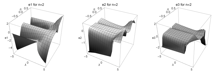
Figure 1: Qualitative evolution for the real part for eigenvalues of the linearized system near to point $P_{5}$. Plots correspond to the eigenvalues for $n=2$. We observe that points $P_{5}~{}$are attractor for $\lambda<3$.

For point $P_{6}$ the eigenvalues of the linearized system are all equal to zero, that is,$~{}e_{1}\left(P_{6}\right)=0,~{}e_{2}\left(P_{6}\right)=0$ and $e_{3}\left(P_{6}\right)=0$. In order to infer on the stability of the stationary points the CMT should be applied. However, in this work we prefer to present the phase-space diagrams where we find that the points are saddle.

Specifically, in Figs. 2 we present the qualitative evolution of the physical parameter $w_{eff}$ and of $x\left(\omega\right),~{}\eta\left(\omega\right)$ for different values of the variable $\lambda$ and for $n=-2$, $\Lambda_{0}=1$. The phase space portraits are given in Fig. 3. It is clear that for $\lambda<3,$ the final attractor is point $P_{3},~{}$while for $\lambda>3$ the final attractor is the de Sitter points $P_{5}$. For $n<0$, it is clear from the phase space that the line $\eta=0$ can not be crossed.

Similarly, for $n=-2$, and for $\Lambda_{0}=1$, the qualitative evolution of the physical parameters and the phase-space portraits are presented in Figs. 3 and 4. There it is clear that the final attractor is always the de Sitter universes described by $P_{5}$. From the plots, it is clear that the Minkowski point $P_{6}$ is a saddle point.

From the phase-space diagrams it is clear that there are trajectories which take values at the infinity for the variable $x$. In the following, we present the the analysis for the existence of stationary points at the infinity.

Figure 2: Qualitative evolution for the physical variable $w_{eff}$ and for the parameters $x,~{}\eta$ for $n=-2,~{}\Lambda_{0}=1$ and for different values of $\lambda$. We observe that the final attractor is point $P_{3}$ for $\lambda<3$, and $P_{5}$ for $\lambda>3$.

Figure 3: Phase-space portrait for the two-dimensional dynamical system in the variables $\left\{x,\eta\right\}$ for the values of the free parameters described in Fig. 2.

Figure 4: Qualitative evolution for the physical variable $w_{eff}$ and for the parameters $x,~{}\eta$ for $n=2,~{}\Lambda_{0}=1$ and for different values of $\lambda$. We observe that the final attractor is always the de Sitter universe of point $P_{5}$

Figure 5: Phase-space portrait for the two-dimensional dynamical system in the variables $\left\{x,\eta\right\}$ for the values of the free parameters described in Fig. 4.

III.3 Analysis at infinity

We continue by studying the evolution of the system at infinity. Parameter $\eta$ is bounded, but that is not true for parameter $x$ which can take values at infinity. This part of the investigation has not been performed before in cel1 .

We do the change of variables $x=\frac{X}{\sqrt{1-X^{2}}}$, $d\varpi=\sqrt{1-X^{2}}d\omega$, where we study the dynamical system for $X=\pm 1$. In the following we consider the case $X=1$. In the new variables the field equations are written as

$$\frac{dX}{d\varpi} =0~{},~{}$$ (29)

$$\frac{d\eta}{d\varpi} =-\lambda\eta^{2}\left(1-\eta^{2}\right).$$ (30)

Hence, the stationary points are for $\eta=\pm 1$ and $\eta=0$. For $\eta=\pm 1$, from the second equation we derive that near the stationary point $\frac{d\eta}{d\varpi}|_{\eta\rightarrow 1}=\pm 2\lambda$. On the other hand, for the Minkowski points we derive $\frac{d\eta}{d\varpi}=0$. Furthermore, can be solved by quadratures.  We perform the second change of variable $d\varpi=\eta d\sigma$, that is, from (30) it follows

$$\eta\left(\sigma\right)=\left(1+e^{2\lambda\sigma}\right)^{-1}\text{. }$$ (31)

Hence, for $\lambda>0$, $\eta=0$ is a future attractor while for $\eta<1$, $\eta=1$ is a future attractor, for equation (30).

Figure 6: Phase-space portrait for the two-dimensional dynamical system (29), (30) in the variables $\left\{X,\eta\right\}$. We observe that at the infinity, $X^{2}=1$, the stationary points are saddle points or sources. Attractors exist only in the finite regime, $X^{2}<1$. The phase-space portraits are for values of the free parameters as presented in Figs. 3 and 5.

IV Conclusions

The determination of the stationary points and the study of their stability is an important approach in order to understand the cosmological evolution and the validity of a specific theory of gravity. In this work we investigated the global dynamics for the fourth-order teleparallel $f\left(T,B\right)$ theory of gravity in a spatially flat FLRW background space. The approach that we applied is more general than that of the Hubble normalization, where we found that Minkowski spacetime can be an exact solution for the field equation described by a stationary point.

In this analysis firstly we wrote the second-order field equations into a system of algebraic-differential equation with the use of new dimensionless variables. The stationary points of the algebraic-differential system were investigated in the local variables as also in the infinite regime. For the functional for of $f\left(T,B\right)$ we assumed $f\left(T,B\right)=F\left(T\right)+\beta\left(B\right)$, in which $F\left(T\right)=T+\Lambda_{0}T^{n}$ and $\beta\left(B\right)=-\frac{B}{\lambda}\ln\left(B\right)$. These two functions reduce the algebraic-differential system into a system of two first-order ordinary differential equations. From previous studies it is known that such $\beta\left(B\right)$ function provides dynamical terms in the field equations that can describe important areas of the cosmological history angrg . Furthermore, for $B=B_{0}>0$, $\beta\left(B\right)$ is approximated as $\beta\left(B\right)\simeq\left(B-B_{0}\right)+\frac{1}{2}\left(B-B_{0}\right)^{2}-\frac{1}{3!}\left(B-B_{0}\right)^{3}+...$. Furthermore, function $F\left(T\right)=T+\Lambda_{0}T^{n}$ has been widely studied in the literature before as a dark energy candidate and there are many applications in the literature Ferraro .

In the finite regime, that is, in the local variables we find that the cosmological field equations admit six stationary points. Points $P_{1},~{}P_{2}$, describe asymptotic solutions where the effective fluid is that of the stiff fluid. Points $P_{3}$ and $P_{4}$ correspond to ideal gas solutions, or to the de Sitter universe for $\lambda=3$. Point $P_{5}$ describes a new family of de Sitter universes, while $P_{6}$ corresponds to the Minkowski universe which is always a saddle point. For these points only one of the points $P_{3}$,$~{}P_{4}$ or $P_{5}$ can be an attractor. That means, that the model can describe a cosmological evolution with at least two expansion eras, a scaling solution and an de Sitter universe, or we can say that it can describes the late time acceleration phase of the universe and an additional matter epoch. It is clear that in order to have all the complete cosmological history, such as radiation and matter eras additional matter source should be considered. However, from these results it is clear that this cosmological model is viable. In addition, we studied the dynamics at the infinite, where we found that no new attractors exists.

This analysis supports the statement that in terms of the background equations $f\left(T,B\right)$ can play an important role for the description for some important eras of the cosmological history. In a future study we plan to investigate the effects of the curvature term in the background space to the field equations.

- (1) E. Di Valentino, O. Mean, S. Pan, L. Visinelli, W. Yang, A. Melchiorri, D.F. Mota, A.G. Riess and J. Silk, In the Realm of the Hubble tension - a Review of Solutions, (2021) [arXiv:2103.01183]
- (2) S. Tsujikawa, Phys. Rev. D 77, 023507 (2008)
- (3) J.W. Moffat and V.T. Toth, Galaxies 1, 65 (2013)
- (4) R.C. Nunes, JCAP 05, 052 (2018)
- (5) S.D. Odintsov, D. Sáez-Chillón Gómez and G.S. Sharov, Nucl. Phys. B 966, 115377 (2021)
- (6) R.C. Nunes, A. Bonilla, S. Pan and E.N. Saridakis, EPJC 77, 230 (2016)
- (7) F.K. Anagnostopoulos, S. Basilakos and E.N. Saridakis, Rev. D 100, 083517 (2019)
- (8) F.K. Anagnostopoulos, S. Basilakos and E.N. Saridakis, First evidence that non-metricity f(Q) gravity can challenge ËCDM, (2021) [arXiv:2104.15123]
- (9) R. Solanki, S.K.J. Pacif, A. Parida and P.K. Sahoo, Phys. Dark Energy 32, 100820 (2021)
- (10) S.I. Nojiri and S.D. Odintsov,IJGMMP 4, 115 (2007)
- (11) T. Harko, F.S.N. Lobo, S. Nojiri and S.D. Odintsov,Phys. Rev. D 84, 024020 (2011)
- (12) S. Nojiri and S.D. Odintsov, Phys. Rev. D 74, 086005 (2005)
- (13) W. Khyllep, A. Paliathanasis and J. Dutta, Phy. Rev. D 103, 103521 (2021)
- (14) R.C. Nunes, S. Pan, E.N. Saridakis and E.M.C. Abreu, JCAP 1701, 005 (2017)
- (15) A.R.P. Moreira, J.E.G. Silva and C.A.S. Almeida, arXiv:2104.00195
- (16) S. Nojiri, S.D. Odintsov and V.K. Oikonomou, Phys. Rept. 692, 1 (2017)
- (17) S.D. Odintsov, V.K. Oikonomou and F.P. Fronimos, Nucl. Phys. B 958, 115135 (2020)
- (18) S.D. Odintsov and V.K. Oikonomou, Phys. Lett. B 805, 135437 (2020)
- (19) S.D. Odintsov and V.K. Oikonomou, Nucl. Phys. 929, 79 (2018)
- (20) A.V. Astashenok, S.D. Odintsov and V.K. Oikonomou, Class. Quantum Grav. 32, 185007 (2015)
- (21) A. Paliathanasis, J.D Barrow and P.G.L. Leach, Phys. Rev. D 94, 023525 (2016)
- (22) H.A. Buchdahl, Mon. Not. Roy. Astron. Soc. 150, 1 (1970)
- (23) S. Bahamonde, C. G. Bohmer and M. Wright, Phys. Rev. D 92, 104042 (2015)
- (24) R. Myrzakulov, FRW Cosmology in F(R,T) gravity, EPJC 72, 1 (2012)
- (25) A. Einstein 1928, Sitz. Preuss. Akad. Wiss. p. 217; ibid p. 224; A. Unzicker and T. Case, Translation of Einstein’s attempt of a unified field theory with teleparallelism, (2005) [physics/0503046]
- (26) K. Hayashi and T. Shirafuji, Phys. Rev. D 19, 3524 (1979)
- (27) G. Bengochea and R. Ferraro, Phys. Rev. D. 79, 124019 (2009).
- (28) G. Farrugia, J.L. Said and A. Finch, Universe, 6, 34 (2020)
- (29) M. Caruana, G. Farrugia and J.L. Said, EPJC 80, 640 (2020)
- (30) S. Bahamonde, V. Gaskis, S. Kiorpelidi, T. Koivisto and J.L. Said, EPJC 81, 53 (2021)
- (31) A. Paliathanasis, Phys. Rev. D 95, 064062 (2017)
- (32) A. Paliathanasis, Universe 7, 150 (2021)
- (33) A. Paliathanasis, JCAP 08, 027 (2017)
- (34) L. Karpathopoulos, S. Basilakos, G. Leon, A. Paliathanasis and M. Tsamparlis, Gen. Rel. Gravit. 50, 79 (2018)
- (35) G.A. Rave Franco, C. Escamilla-River and J.L. Said, EPJC 80, 677 (2020)
- (36) G.A. Rave Franco, C. Escamilla-River and J.L. Said, Phys. Rev. D 103, 084017 (2021)
- (37) J. W. Maluf, J. Math. Phys. 35, 335 (1994)
- (38) H. I. Arcos and J. G. Pereira, Int. J. Mod. Phys. D 13, 2193 (2004)
- (39) C.-Q. Geng, C.-C. Lee, E.N. Saridakis and Y.-P. Wu, Phys. Lett. B 704, 384 (2011)
- (40) M. Wright, Phys. Rev. D 93, 103002 (2016)
- (41) G.R. Bengochea, Phys. Lett. B 695, 405 (2011)
- (42) S. Basilakos, Phys. Rev. D 93, 083007 (2016)
- (43) E.J. Copeland, A.R. Liddle and D. Wands, Phys. Rev. D. 57, 4686 (1998)
- (44) A. Paliathanasis, M. Tsampalis, S. Basilakos and J.D. Barrow, Phys. Rev. D 91, 123535 (2015)
- (45) L. Amendola, D. Polarski and S. Tsujikawa, IJMPD 16, 1555 (2007)
- (46) G. Leon and E.N. Saridakis, JCAP 1504, 031 (2015)
- (47) H. Farajollahi and A. Salehi, JCAP 07, 036 (2011)
- (48) M. Kerachian, G. Acquaviva and G. Lukes-Gerakopoulos, Phys. Rev. D 101, 043535 (202)
- (49) S. Mishra and S. Chakraborty, EPJC 79, 328 (2019)
- (50) R. Lazkoz and G. Leon, Phys. Lett. B 638, 303 (2006)
- (51) T. Gonzales, G. Leon and I. Quiros, Class. Quantum Grav. 23, 3165 (2006)
- (52) A. Giacomini, S. Jamal, G. Leon, A. Paliathanasis and J. Saveedra, Phys. Rev. D 95, 124060 (2017)