Linear-Time Gromov Wasserstein Distances
using Low Rank Couplings and Costs

Abstract

The ability to align points across two related yet incomparable point clouds (e.g. living in different spaces) plays an important role in machine learning. The Gromov-Wasserstein (GW) framework provides an increasingly popular answer to such problems, by seeking a low-distortion, geometry-preserving assignment between these points. As a non-convex, quadratic generalization of optimal transport (OT), GW is NP-hard. While practitioners often resort to solving GW approximately as a nested sequence of entropy-regularized OT problems, the cubic complexity (in the number $n$ of samples) of that approach is a roadblock. We show in this work how a recent variant of the OT problem that restricts the set of admissible couplings to those having a low-rank factorization is remarkably well suited to the resolution of GW: when applied to GW, we show that this approach is not only able to compute a stationary point of the GW problem in time $O(n^{2})$, but also uniquely positioned to benefit from the knowledge that the initial cost matrices are low-rank, to yield a linear time $O(n)$ GW approximation. Our approach yields similar results, yet orders of magnitude faster computation than the SoTA entropic GW approaches, on both simulated and real data.

1 Introduction

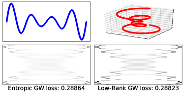
Figure 1: Top row: Two curves in 2D and 3D, with $n=5000$ points. Bottom row: coupling and GW loss obtained with the SoTA $O(n^{3})$ entropic approach (Peyré et al., 2016) (left) and with our linear $O(n)$ method (right) when using the squared Euclidean distances as the ground costs.

Increasing interest for Gromov-Wasserstein… Several problems in machine learning require comparing datasets that live in heterogeneous spaces. This situation arises typically when realigning two distinct views (or features) from points sampled from similar sources. Recent applications to single-cell genomics (Demetci et al., 2020; Blumberg et al., 2020) provide a case in point: Thousands of cells taken from the same tissue are split in two groups, each processed with a different experimental protocol, resulting in two distinct sets of heterogeneous feature vectors; Despite this heterogeneity, one expects to find a mapping registering points from the first to the second set, since they contain similar overall information. That realignment is usually carried out using the Gromov-Wasserstein (GW) machinery proposed by Mémoli (2011) and  Sturm (2012). GW seeks a relaxed assignment matrix that is as close to an isometry as possible, as quantified by a quadratic score. GW has practical appeal: It has been used in supervised learning (Xu et al., 2019b), generative modeling (Bunne et al., 2019), domain adaptation (Chapel et al., 2020), structured prediction (Vayer et al., 2018), quantum chemistry (Peyré et al., 2016) and alignment layers (Ezuz et al., 2017).

…despite being hard to solve. Since GW is an NP-hard problem, all applications above rely on heuristics, the most popular being the sequential resolution of nested entropy-regularized OT problems. That approximation remains costly, requiring $\mathcal{O}(n^{3})$ operations when dealing with two datasets of $n$ samples. Our goal is to reduce that complexity, by exploiting and/or enforcing low-rank properties of matrices arising both in data and variables of the GW problem.

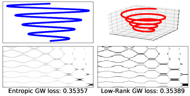
Figure 2: Top row: Two curves in 2D and 3D, with $n=5000$ points. Bottom row: coupling and GW loss obtained with the SoTA $O(n^{3})$ entropic approach (Peyré et al., 2016) (left) and with our linear $O(n)$ method (right) when using the squared Euclidean distance as the ground cost for both point clouds. See Appendix E.1 for more details.

OT: from cubic to linear complexity. Compared to GW, aligning two populations embedded in the same space is far simpler, and corresponds to the usual optimal transport (OT) problem (Peyré and Cuturi, 2019).Given a $n\times m$ cost matrix $C$ and two marginals, the OT problem minimizes $\mathcal{L}_{C}(P):=\langle C,P\rangle$ w.r.t. a coupling matrix $P$ satisfying these marginal constraints. For computational and statistical reasons, most practitioners rely on regularized approaches $\mathcal{L}^{\varepsilon}_{C}(P):=\langle C,P\rangle+\varepsilon\text{reg}(P)$. When reg is the neg-entropy, Sinkhorn’s algorithm can be efficiently employed (Cuturi, 2013; Altschuler et al., 2017; Lin et al., 2019). The Sinkhorn iteration has $O(nm)$ complexity, but this can be sped-up using either a low-rank factorizations (or approximations) of the kernel matrix $K:=e^{-C/\varepsilon}$ (Solomon et al., 2015; Altschuler et al., 2018a, b; Scetbon and Cuturi, 2020), or, alternatively and as proposed by Scetbon et al. (2021); Forrow et al. (2019), by imposing a low-rank constraint on the coupling $P$. A goal in this paper is to show that this latter route is remarkably well suited to the GW problem.

GW: from NP-hard to cubic approximations. The GW problem replaces the linear objective in OT by a non-convex, quadratic, objective $\mathcal{Q}_{A,B}(P):=\text{cst}-2\langle APB,P\rangle$ parameterized by two square cost matrices $A$ and $B$. Much like OT is a relaxation of the optimal assignment problem, GW is a relaxation of the quadratic assignment problem (QAP). Both GW and QAP are NP-hard (Burkard et al., 1998). In practice, linearizing iteratively $\mathcal{Q}_{A,B}$ works well (Gold and Rangarajan, 1996; Solomon et al., 2016): recompute a synthetic cost $C_{t}:=AP_{t-1}B$, use Sinkhorn to get $P_{t}:=\operatorname*{argmin}_{P}\langle C_{t},P\rangle+\varepsilon\text{reg}(P)$, repeat. This is akin to a mirror-descent scheme (Peyré et al., 2016), interpreted as a bi-linear relaxation in certain cases (Konno, 1976).

Challenges to speed up GW. Several obstacles stand in the way of speeding up GW. The re-computation of $C_{t}=AP_{t-1}B$ at each outer iteration is an issue, since it requires $O(n^{3})$ operations (Peyré et al., 2016, Prop. 1). We only know of two broad approaches that achieve tractable running times: (i) Solve related, yet significantly different, proxies of the GW energy, either by embedding points as univariate measures (Mémoli, 2011; Sato et al., 2020), by using a sliced mechanism when restricted to Euclidean settings (Vayer et al., 2019) or by considering tree metrics for supports of each probability measure (Le et al., 2021), (ii) Reduce the size of the GW problem through quantization of input measures (Chowdhury et al., 2021). or recursive clustering approaches (Xu et al., 2019a; Blumberg et al., 2020)). Interestingly, no work has, to our knowledge, tried yet to accelerate Sinkhorn iterations withing GW.

Our contributions: a quadratic to linear GW approximation. Our method addresses the problem by taking the GW as it is, overcoming limitations that may arise from a changing cost matrix $C_{t}$. We show first that a low-rank factorization (or approximation) of the two input cost matrices that define GW, one for each measure, can be exploited to lower the complexity of recomputing $C_{t}$ from cubic to quadratic. We show next, independently, that using the low-rank approach for couplings advocated by Scetbon et al. (2021) to solve OT can be inserted in the GW pipeline and result in a $O(n^{2})$ strategy for GW, with no prior assumption on input cost matrices. We also briefly explain why methods that exploit the geometrical properties of $C$ (or its kernel $K=e^{-C}$) to obtain faster iterations are of little use in a GW setup, because of the necessity to re-instantiate a new cost $C_{t}$ at each outer iteration. Finally, we show that both low-rank assumptions (on costs and couplings) can be combined to shave yet another factor and reach GW approximation with linear complexity in time and memory. We provide experiments, on simulated and real datasets, which show that our approach has comparable performance to entropic-regularized GW and its practical ability to reach “good” local minima to GW, for a considerably cheaper computational price, and with a conceptually different regularization path (see Fig. 1,2), yet can scale to millions of points.

2 Background on Gromov-Wasserstein

Comparing measured metric spaces. Let $(\mathcal{X},d_{\mathcal{X}})$ and $(\mathcal{Y},d_{\mathcal{Y}})$ be two metric spaces, and $\mu:=\sum_{i=1}^{n}a_{i}\delta_{x_{i}}$ and $\nu:=\sum_{i=j}^{m}b_{j}\delta_{y_{j}}$ two discrete probability measures, where $n,m\geq 1$; $a$, $b$ are probability vectors in the simplicies $\Delta_{n},\Delta_{m}$ of size $n$ and $m$; and $(x_{1},\dots,x_{n})$, $(y_{1},\dots,y_{m})$ are families in $\mathcal{X}$ and $\mathcal{Y}$. Given $q\geq 1$, the following square pairwise cost matrices encode the geometry within $\mu$ and $\nu$,

$$A:=[d_{\mathcal{X}}^{q}(x_{i},x_{i^{\prime}})]_{1\leq i,i^{\prime}\leq n},\;B:=[d_{\mathcal{Y}}^{q}(x_{j},x_{j^{\prime}})]_{1\leq i,i^{\prime}\leq m}\,$$

The GW discrepancy between these two discrete metric measure spaces $(\mu,d_{\mathcal{X}})$ and $(\nu,d_{\mathcal{Y}})$ is the solution of the following non-convex quadratic problem, written for simplicity as a function of $(a,A)$ and $(b,B)$:

$$\text{GW}((a,A),(b,B))=\!\!\min_{P\in\Pi_{a,b}}\!\!\mathcal{Q}_{A,B}(P),\,$$ (1)

$$\text{where }\Pi_{a,b}:=\{P\in\mathbb{R}_{+}^{n\times m}|P\mathbf{1}_{m}=a,P^{T}\mathbf{1}_{n}=b\},$$

and the energy $\mathcal{Q}_{A,B}$ is a quadratic function of $P$ designed to measure the distortion of the assignment:

$$\mathcal{Q}_{A,B}(P):=\sum_{i,j,i^{\prime},j^{\prime}}(A_{i,i^{\prime}}-B_{j,j^{\prime}})^{2}P_{i,j}P_{i^{\prime},j^{\prime}}\;.$$ (2)

Mémoli (2011) proves that $\text{GW}^{\tfrac{1}{2}}$ defines a distance on the space of metric measure spaces quotiented by measure-preserving isometries.  (2) can be evaluated in $\mathcal{O}(n^{2}m+nm^{2})$ operations, rather than using $n^{2}m^{2}$ terms:

$$\mathcal{Q}_{A,B}(P)=\langle A^{\odot 2}a,a\rangle+\langle B^{\odot 2}b,b\rangle-2\langle APB,P\rangle\;,$$ (3)

where $\odot$ is the Hadamard (elementwise) product or power.

Entropic Gromov-Wasserstein. The original GW problem (1) can be regularized using entropy  (Gold and Rangarajan, 1996; Solomon et al., 2016), leading to problem:

$$\text{GW}_{\varepsilon}((a,A),(b,B))=\min_{P\in\Pi_{a,b}}\mathcal{Q}_{A,B}(P)-\varepsilon H(P)\,,$$ (4)

where $H(P):=-\sum_{i,j}P_{i,j}(\log(P_{i,j})-1)$ is $P$’s entropy. Peyré et al. (2016) propose to solve that problem using mirror descent (MD), w.r.t. the KL divergence. Their algorithm boils down to solving a sequence of regularized OT problems, as in Algo. 1: Each KL projection in Line 1 is solved efficiently with the Sinkhorn algorithm (Cuturi, 2013).

Input :

$a\in\Delta_{n},A\in\mathbb{R}^{n\times n}\!\!,b\in\Delta_{m},B\in\mathbb{R}^{m\times m}\!\!,\varepsilon>0$

$P=ab^{T}$ nm
for $t=0,\dots$ do

2       $C\leftarrow-4APB$  nm(n+m)
$K_{\varepsilon}\leftarrow\exp(-C/\varepsilon)$ nm
$P\leftarrow\operatorname*{argmin}\limits_{P\in\Pi(a,b)}\text{KL}(P,K_{\varepsilon})$ $\mathcal{O}$(nm)

$\text{GW}=\mathcal{Q}_{A,B}(P)$  nm(n+m)
Result: GW

Algorithm 1 Entropic-GW

Computational complexity. Given a cost matrix $C$, the KL projection of $K_{\varepsilon}$ onto the polytope $\Pi(a,b)$, where $\text{KL}(P,Q)=\langle P,\log(P/Q)-1\rangle$, is carried out in Line 1 of the inner loop of Algo. 1 using the Sinkhorn algorithm, through matrix-vector products. This quadratic complexity (in red) is dominated by the cost of updating matrix $C$ at each iteration in Line 1, which requires $\mathcal{O}(n^{2}m+nm^{2})$ algebraic operations (cubic, in violet). As noted above, evaluating the objective $\mathcal{Q}_{A,B}(P)$ in Line 1 is also cubic.

Step-by-step guide to reaching linearity. We show next in §3 that these iterations can be sped up when the distance matrices are low-rank (or have low-rank approximations), in which case the cubic updates in $C$ and evaluation of $\mathcal{Q}_{A,B}$ in Lines 1, 1 become quadratic. Independently, we show in §4 that, with no assumption on these cost matrices, replacing the Sinkhorn call in Line 1 with a low-rank approach (Scetbon et al., 2021) can lower the cost of Lines 1, 1 to quadratic (while also making Line 1 linear). Remarkably, we show in §5 that these two approaches can be combined in Lines 1, 1, to yield, to the best of our knowledge, the first linear time/memory algorithm able to match the performance of the Entropic-GW approach.

3 Low-rank (Approximated) Costs

Exact factorization for distance matrices. consider

Assumption 1.

$A$ and $B$ admit a low-rank factorization: there exists $A_{1},A_{2}\in\mathbb{R}^{n\times d}$ and $B_{1},B_{2}\in\mathbb{R}^{m\times d^{\prime}}$ s.t. $A=A_{1}A_{2}^{T}$ and $B=B_{1}B_{2}^{T}$, where $d\ll n,d^{\prime}\ll m$.

A case in point is when both $A$ and $B$ are squared Euclidean distance matrices, with a sample size that is much larger than ambient dimension. This case is highly relevant in practice, since it covers most applications of OT to ML. Indeed, the $d\ll n$ assumption usually holds, since cases where $d\gg n$ fall in the “curse of dimensionality” regime where OT is less useful (Dudley et al., 1966; Weed and Bach, 2019). Writing $X=[x_{1},\dots,x_{n}]\in\mathbb{R}^{d\times n}$, if $A=\left[\|x_{i}-x_{j}\|_{2}^{2}\right]_{i,j}$, then one has, writing $z=(X^{\odot 2})^{T}\mathbf{1}_{d}\in\mathbb{R}^{n}$ that $A=z\mathbf{1}_{n}^{T}+\mathbf{1}_{n}z^{T}-2X^{T}X.$ Therefore by denoting $A_{1}=[z,\mathbf{1}_{n},-\sqrt{2}X^{T}]\in\mathbb{R}^{n\times(d+2)}$ and $A_{2}=[\mathbf{1}_{n},z,\sqrt{2}X^{T}]\in\mathbb{R}^{n\times(d+2)}$ we obtain the factorization above. Under Assumption 1, the complexity of Algo. 1 is reduced to $O(n^{2})$: Line 1 reduces to:

$$C=-4A_{1}A_{2}^{T}PB_{1}B_{2}^{T}\,,$$

in $nm(d+d^{\prime})+dd^{\prime}(n+m)$ algebraic operations, while Line 1, using the reformulation of $\mathcal{Q}_{A,B}(P)$ in (3), becomes quadratic as well. Indeed, writing $G_{1}:=A_{1}^{T}PB_{2}$ and $G_{2}:=A_{2}^{T}PB_{1}$, both in $\mathbb{R}^{d\times d^{\prime}}$, one has $\langle APB,P\rangle=\mathbf{1}_{d}^{T}(G_{1}\odot G_{2})\mathbf{1}_{d^{\prime}}$. Computing $G_{1},G_{2}$ given $P$ requires only $2(nmd+mdd^{\prime})$, and computing their dot product adds $dd^{\prime}$ algebraic operations. The overall complexity to compute $\mathcal{Q}_{A,B}(P)$ is $\mathcal{O}(nmd+mdd^{\prime})$.

Inputs: $A_{1},A_{2}\in\mathbb{R}^{n\times d},B_{1},B_{2},\in\mathbb{R}^{m\times d^{\prime}}a,b,\varepsilon$
$P=ab^{T}$     nm
for $t=0,\dots$ do

       $G_{2}\leftarrow A_{2}^{T}PB_{1}$      nmd + mdd’
$C\leftarrow-4A_{1}G_{2}B_{2}^{T}$      nmd’ + ndd’
$K_{\varepsilon}\leftarrow\exp(-C/\varepsilon)$     nm
$P\leftarrow\operatorname*{argmin}\limits_{P\in\Pi(a,b)}\text{KL}(P,K_{\varepsilon})$     $\mathcal{O}$(nm)

end for

$c_{1}\leftarrow a^{T}(A_{1}A_{2}^{T})^{\odot 2}a+b^{T}(B_{1}B_{2}^{T})^{\odot 2}b$    n²d’+m²d’
$G_{2}\leftarrow A_{2}^{T}PB_{1}$      nmd + mdd’
$G_{1}\leftarrow A_{1}^{T}PB_{2}$     nmd + mdd’
$c_{2}\leftarrow-2\mathbf{1}_{d}^{T}(G_{1}\odot G_{2})\mathbf{1}_{d^{\prime}}$     dd’
$\mathcal{Q}_{A,B}(P)\leftarrow c_{1}+c_{2}$
Return: $\mathcal{Q}_{A,B}(P)$

Algorithm 2 Quadratic Entropic-GW

General distance matrices. When the original cost matrices $A,B$ are not low-rank but describe distances, we build upon recent works that output their low-rank approximation in linear time (Bakshi and Woodruff, 2018; Indyk et al., 2019). These algorithms produce, for any distance matrix $A\in\mathbb{R}^{n\times m}$ and $\tau>0$, matrices $A_{1}\in\mathbb{R}^{n\times d}$, $A_{2}\in\mathbb{R}^{m\times d}$ in $\mathcal{O}((m+n)\text{poly}(\frac{d}{\tau}))$ operations such that, with probability at least $0.99$,

$$\|A-A_{1}A_{2}^{T}\|_{F}^{2}\leq\|A-A_{d}\|_{F}^{2}+\tau\|A\|_{F}^{2}\,,$$

where $A_{d}$ denotes the best rank-$d$ approximation to $A$ in the Frobenius sense. The rank $d$ should be selected to trade off approximation of $A$ and speed-ups for the method, e.g. such that $d/\tau\ll m+n$. We fall back on this approach to obtain a low-rank factorization of a distance matrix in linear time whenever needed, aware that this incurs an additional approximation (see Appendix C).

4 Low-rank Constraints for Couplings

In this section, we shift our attention to a different opportunity for speed-ups, without Assumption 1: we consider the GW problem on couplings that are low-rank, in the sense that they are factorized using two low-rank couplings linked by a common marginal $g$ in $\Delta_{r}^{*}$, the interior of $\Delta_{r}$ (all entries positive). Writing the set of couplings with a nonnegative rank smaller than $r$ (Scetbon et al., 2021, §3.1):

$$\Pi_{a,b}(r):=\begin{aligned} \Big{\{}&P\in\mathbb{R}_{+}^{n\times m},\exists g\in\Delta_{r}^{*}\text{~{}s.t.~{}}P=Q\operatorname{diag}(1/g)R^{T},\\ &Q\in\Pi_{a,g},\text{ and }R\in\Pi_{b,g}\Big{\}}\;,\end{aligned}$$

we can define the low-rank GW problem, written $\text{GW-LR}^{(r)}((a,A),(b,B))$ as the solution of

$$\min_{(Q,R,g)\in\mathcal{C}(a,b,r)}\mathcal{Q}_{A,B}(Q\operatorname{diag}(1/g)R^{T})\,,$$ (5)

where $\mathcal{C}(a,b,r):=\mathcal{C}_{1}(a,b,r)\cap\mathcal{C}_{2}(r)$, with

$$\mathcal{C}_{1}(a,b,r) :=\begin{aligned} \Big{\{}&(Q,R,g)\in\mathbb{R}_{+}^{n\times r}\times\mathbb{R}_{+}^{m\times r}\times(\mathbb{R}_{+}^{*})^{r}\\ &\text{ s.t. }Q\mathbf{1}_{r}=a,R\mathbf{1}_{r}=b\Big{\}}\,,\end{aligned}$$

$$\mathcal{C}_{2}(r) :=\begin{aligned} \Big{\{}&(Q,R,g)\in\mathbb{R}_{+}^{n\times r}\times\mathbb{R}_{+}^{m\times r}\times\mathbb{R}^{r}_{+}\\ &\text{ s.t. }Q^{T}\mathbf{1}_{n}=R^{T}\mathbf{1}_{m}=g\Big{\}}.\end{aligned}$$

Mirror Descent Scheme. We propose to use a MD scheme with respect to the generalized KL divergence to solve (5). If one chooses $(Q_{0},R_{0},g_{0})\in\mathcal{C}(a,b,r)$ an initial point such that $Q_{0}>0$ and $R_{0}>0$, this results in,

$$(Q_{k+1},R_{k+1},g_{k+1}):=\!\!\operatorname*{argmin}_{\zeta\in\mathcal{C}(a,b,r)}\!\!\text{KL}(\zeta,K_{k})\;,$$ (6)

where the three matrices $K_{k}:=(K_{k}^{(1)},K_{k}^{(2)},K_{k}^{(3)})$ are

$$K_{k}^{(1)} :=\exp(4\gamma AP_{k}BR_{k}\operatorname{diag}(1/g_{k})+\log(Q_{k}))$$

$$K_{k}^{(2)} :=\exp(4\gamma BP^{T}_{k}AQ_{k}\operatorname{diag}(1/g_{k})+\log(R_{k}))$$

$$K_{k}^{(3)} :=\exp(-4\gamma\omega_{k}/g_{k}^{2}+\log(g_{k}))$$

with $[\omega_{k}]_{i}:=[Q_{k}^{T}AP_{k}BR_{k}]_{i,i}$ for all $i\in\{1,\dots,r\}$ and $\gamma>0$ is a step size. Solving (6) can be done efficiently thanks to Dykstra’s Algorithm as proposed in (Scetbon et al., 2021). See Algo. 3 and Appendix D.

Avoiding vanishing components. As in $k$-means optimization, the algorithm above might run into cases in which entries of the histogram $g$ vanish to $0$. Following  (Scetbon et al., 2021) we can avoid this by setting a lower bound $\alpha$ on the weight vector $g$, such that $g\geq\alpha$ coordinate-wise. Practically, we introduce truncated feasible sets $\mathcal{C}(a,b,r,\alpha):=\mathcal{C}_{1}(a,b,r,\alpha)\cap\mathcal{C}_{2}(r)$ where $\mathcal{C}_{1}(a,b,r,\alpha):=\mathcal{C}_{1}(a,b,r)\cap\{(Q,R,g)~{}|~{}g\geq\alpha\}$.

Initialization. To initialize our algorithm, we adapt the first lower bound of (Mémoli, 2011) to the low-rank setting and prove the following Proposition (see appendix A for proof).

Proposition 1.

Let us denote $\tilde{x}=A^{\odot 2}a\in\mathbb{R}^{n}$, $\tilde{y}=B^{\odot 2}b\in\mathbb{R}^{m}$ and $\tilde{C}=(|\sqrt{\tilde{x}_{i}}-\sqrt{\tilde{y}_{j}}|^{2})_{i,j}\in\mathbb{R}^{n\times m}$. Then for all $r\geq 1$ we have,

$$\text{GW-LR}^{(r)}_{\alpha}((a,A),(b,B))\geq\text{LOT}^{(r)}_{\alpha}(\tilde{C},a,b),\text{where}$$

$$\text{LOT}^{(r)}_{\alpha}(\tilde{C},a,b):=\min_{(Q,R,g)\in\mathcal{C}(a,b,r,\alpha)}\langle\tilde{C},Q\operatorname{diag}(1/g)R^{T}\rangle\;.$$

$\text{LOT}^{(r)}_{\alpha}(\tilde{C},a,b)$ can be solved with (Scetbon et al., 2021). The cost $\tilde{C}$ is the squared Euclidean distance between two families $\{\tilde{x}_{1},\dots,\tilde{x}_{n}\}$ and $\{\tilde{y}_{1},\dots,\tilde{y}_{m}\}$ in 1-D, which admits a trivial rank 2 factorization. We can therefore apply the linear-time version of their algorithm to compute the lower bound. Algo. 3 summarizes this, where $\mathcal{D}(\cdot)$ denotes the operator extracting the diagonal of a square matrix. In practice we observe that such initialization outperforms trivial or random initializations (see Section 6).

Computational Cost. Our initialization requires $\tilde{x}$ and $\tilde{y}$, obtained in $\mathcal{O}(n^{2}+m^{2})$ operations. Running  (Scetbon et al., 2021, Algo.3) with a squared Euclidean distances between two families in 1-D has cost $\mathcal{O}((n+m)r)$. Solving the barycenter problem as defined in (6) can be done efficiently thanks to Dykstra’s Algorithm. Indeed, each iteration of (Scetbon et al., 2021, Algo. 2), assuming $(K^{(1)}_{k},K^{(2)}_{k},K^{(3)}_{k})$ is given, requires only $\mathcal{O}((n+m)r)$ algebraic operations. However, computing kernel matrices $(K^{(1)}_{k},K^{(2)}_{k},K^{(3)}_{k})$ at each iteration of Algorithm 3 requires a quadratic complexity with respect to the number of samples. Overall the proposed algorithm, while faster than the cubic implementation proposed in (Peyré et al., 2016), still needs $\mathcal{O}((n^{2}+m^{2})r)$ operations per iteration.

Dykstra Iterations. In our complexity analysis, we do not take into account the number of iterations required to terminate Dykstra’s Algorithm. We show experimentally (see Fig. 3) that, as usually observed for Sinkhorn (Cuturi, 2013, Fig. 5), this number does not depend on problem size $n,m$, but rather on the geometric characteristics of $A,B$ and $\gamma$.

Convergence of MD. Although objective (5) is not convex in $(Q,R,g)$, we obtain the non-asymptotic stationary convergence of our proposed method. In (Scetbon et al., 2021), the authors study the convergence of the MD scheme when applied to the low-rank formulation of OT. In the GW setting, such strategy makes even more sense as the GW problem is a NP-hard non-convex problem and obtaining global guarantees is out of reach in a general framework. Therefore we follow the strategy proposed in (Scetbon et al., 2021) and consider the following convergence criterion,

$$\Delta_{\alpha}(\xi,\gamma):=\frac{1}{\gamma^{2}}(\text{KL}(\xi,\mathcal{G}_{\alpha}(\xi,\gamma))+\text{KL}(\mathcal{G}_{\alpha}(\xi,\gamma),\xi))$$

where $\mathcal{G}_{\alpha}(\xi,\gamma):=\operatorname*{argmin}_{\zeta\in\mathcal{C}(a,b,r,\alpha)}\{\langle\nabla\mathcal{Q}_{A,B}(\xi),\zeta\rangle+\frac{1}{\gamma}\text{KL}(\zeta,\xi)\}.$ This convergence criterion is in fact stronger than the one using the (generalized) projected gradient presented in (Ghadimi et al., 2013) to obtain non-asymptotic stationary convergence of the MD scheme. Indeed the criterion used there is defined as the square norm of the following vector:

$$P_{\mathcal{C}(a,b,r,\alpha)}(\xi,\gamma):=\frac{1}{\gamma}(\xi-\mathcal{G}_{\alpha}(\xi,\gamma))\;,$$

which can be seen as a generalized projected gradient of $\mathcal{Q}_{A,B}$ at $\xi$. By denoting $X:=\mathbb{R}^{d}$ and by replacing the Bregman Divergence $\text{KL}(\zeta,\xi)$ by $\frac{1}{2}\|\zeta-\xi\|_{2}^{2}$ in the MD scheme, we would have $P_{X}(\xi,\gamma)=\nabla\mathcal{Q}_{A,B}(\xi)$. Now observe that we have

$$\Delta_{\alpha}(\xi,\gamma) =\frac{1}{\gamma^{2}}(\langle\nabla h(\mathcal{G}_{\alpha}(\xi,\gamma))-\nabla h(\xi),\mathcal{G}_{\alpha}(\xi,\gamma)-\xi\rangle$$

$$\geq\frac{1}{2\gamma^{2}}\|\mathcal{G}_{\alpha}(\xi,\gamma)-\xi\|_{1}^{2}$$

$$=\frac{1}{2}\|P_{\mathcal{C}(a,b,r,\alpha)}(\xi,\gamma)\|_{1}^{2}$$

where $h$ denotes the minus entropy function and the last inequality comes from the strong convexity of $h$ on $\mathcal{C}(a,b,r,\alpha)$. Therefore $\Delta_{\alpha}(\xi,\gamma)$ dominates $\|P_{\mathcal{C}(a,b,r,\alpha)}(\xi,\gamma)\|_{1}$ and characterizes a stronger convergence.

For any $1/r\geq\alpha>0$, Proposition 2 shows the non-asymptotic stationary convergence of the MD scheme for Problem (5). See Appendix A for the proof.

Proposition 2.

Let $\frac{1}{r}\geq\alpha>0,N\geq 1$ and $L_{\alpha}:=27(\|A\|_{2}\|B\|_{2}/\alpha^{4})$. Consider a constant stepsize $\gamma=\frac{1}{2L_{\alpha}}$ in the MD scheme (6). Writing $D_{0}:=\mathcal{Q}_{A,B}(Q_{0}\operatorname{diag}(1/g_{0})R_{0}^{T})-\text{{GW-LR}}^{(r)}_{\alpha}((a,A),(b,B))$ the gap between initial value and optimum, one has

$$\min_{1\leq k\leq N}\Delta_{\alpha}((Q_{k},R_{k},g_{k}),\gamma)\leq\frac{4L_{\alpha}D_{0}}{N}.$$

Since for $\alpha$ small enough, $\text{GW-LR}^{(r)}_{\alpha}((a,A),(b,B))=\text{GW-LR}^{(r)}((a,A),(b,B))$, Proposition 2 shows that our algorithm reaches a stationary point of (5).

This Proposition claims that within at most $N$ iterations the minimum of the $(\Delta_{\alpha}((Q_{t},R_{t},g_{t}),\gamma))_{1\leq t\leq N}$ is of order $\mathcal{O}(1/N)$. Note that this is a standard way to obtain the stationary convergence (see e.g. (Ghadimi et al., 2013). In practice, this is sufficient to define a stopping criteria, as one could simply compute at each iteration the criterion and keep only in memory the smallest value at each iteration.

Inputs: $A,B,a,b,r,\alpha,\gamma$
$\tilde{x}\leftarrow A^{\odot 2}a$, $\tilde{y}\leftarrow B^{\odot 2}b$      $\mathtt{m^{2}+n^{2}}$
$z_{1}\leftarrow\tilde{x}^{\odot 2}$, $z_{2}\leftarrow\tilde{y}^{\odot 2}$      $\mathtt{m+n}$
$\tilde{C}_{1}\leftarrow[z_{1},\mathbf{1}_{n},-\sqrt{2}\tilde{x}]$, $\tilde{C}_{2}\leftarrow[\mathbf{1}_{m},z_{2},\sqrt{2}\tilde{y}]^{T}$      $\mathtt{n+m}$
$(Q,R,g)\leftarrow\text{LOT}^{(r)}_{\alpha}(\tilde{C}_{1}\tilde{C}_{2},a,b)$      $\mathcal{O}(\mathtt{(n+m)r})$
for $t=1,\dots$ do

       $C_{1}\leftarrow-AQ\operatorname{diag}(1/g)$     $\mathcal{O}(\mathtt{n^{2}r})$
$C_{2}\leftarrow R^{T}B$     $\mathcal{O}(\mathtt{m^{2}r})$
$K^{(1)}\leftarrow Q\odot e^{4\gamma C_{1}C_{2}R\operatorname{diag}(1/g)}$  $\mathcal{O}(\mathtt{(m+n)r^{2}})$
$K^{(2)}\leftarrow R\odot e^{4\gamma C_{2}^{T}C_{1}^{T}Q\operatorname{diag}(1/g)}$  $\mathcal{O}(\mathtt{(m+n)r^{2}})$
$\omega\leftarrow\mathcal{D}(Q^{T}C_{1}C_{2}R)$  $\mathcal{O}(\mathtt{nr^{2}})$
$K^{(3)}\leftarrow g\odot e^{-4\gamma\omega/g^{2}}$  $\mathcal{O}(\mathtt{r})$
$Q,R,g\leftarrow\operatorname*{argmin}\limits_{\zeta\in\mathcal{C}(a,b,r,\alpha)}\!\!\text{KL}(\zeta,K)$  $\mathcal{O}(\mathtt{(m+n)r})$

end for

$c_{1}\leftarrow\langle\tilde{x},a\rangle+\langle\tilde{y},b\rangle$     $\mathtt{n+m}$
$C_{1}\leftarrow-AQ\operatorname{diag}(1/g)$     $\mathcal{O}(\mathtt{n^{2}r})$
$C_{2}\leftarrow R^{T}B$     $\mathcal{O}(\mathtt{m^{2}r})$
$G\leftarrow C_{2}R$, $G\leftarrow C_{1}G$     $\mathcal{O}(\mathtt{(m+n)r^{2}})$
$c_{2}\leftarrow-2\langle Q,G\operatorname{diag}(1/g)\rangle$     $\mathcal{O}(\mathtt{nr})$
$\mathcal{Q}\leftarrow c_{1}+c_{2}$
Return: $\mathcal{Q}$

Algorithm 3 Low-Rank GW

5 Double Low-rank GW

Almost all operations in Algorithm 3 only require linear memory storage and time, except for the computations of $\tilde{x}=A^{\odot 2}a$ and $\tilde{y}=B^{\odot 2}b$ in Line 3, and the four updates involving $C_{1}$ and $C_{2}$ in Lines 3,3,3,3 which all require a quadratic number of algebraic operations. When adding Assumption 1 from §3 to the rank constrained approach from §4, we show that the strengths of both approaches can work hand in hand, both in easier initial evaluations of $\tilde{x},\tilde{y}$, but, most importantly, at each new recomputation of a factorized linearization of the quadratic objective:

Linear-time Norms in Line 3 Because $A$ admits a low-rank factorization, one can obtain a low-rank factorization for $A^{\odot 2}$ pending the condition $d^{2}\ll n$. Indeed, remark that for $u,v\in\mathbb{R}^{d},\langle u,v\rangle^{2}=\langle uu^{T},vv^{T}\rangle$. Therefore, if one describes $A_{1}:=[u_{1};\dots;u_{n}]$ and $A_{2}:=[v_{1};\dots;v_{n}]$ row-wise, and one uses the flattened out-product operator $\psi(u):=\text{vec}(uu^{T})\in\mathbb{R}^{d^{2}}$ where $\text{vec}(\cdot)$ flattens a matrix,

$$A^{\odot 2}=\tilde{A_{1}}\tilde{A_{2}}^{T}\text{ where }\tilde{A_{1}} =[\psi(u_{1};\dots;\psi(u_{n})],\;$$

$$\tilde{A_{2}} =[\psi(v_{1});\dots;\psi(v_{n})]\;.$$

Line 3 in Algo. 3 can be replaced by $\tilde{x}\leftarrow\tilde{A_{1}}\tilde{A_{2}}^{T}a$ and $\tilde{y}\leftarrow\tilde{B_{1}}\tilde{B_{2}}^{T}b$. Pending the condition $d^{2}\ll n,d^{\prime 2}\ll m$, this results in $nd^{2}+m(d^{\prime})^{2}$ operations. Note that Algo. 2 (line 2) can also benefit from this factorization, however as its complexity is already quadratic, the linearization of this operation has no effect on the global computational cost.

Linearization of Lines 3,3,3,3. The critical step in Algo. 1 that requires updating $C$ at each outer iteration is cubic. As described earlier in Algo. 3 and Algo. 2, a low-rank constraint on the coupling or a low-rank assumption on costs $A$ and $B$ reduce this cost to quadratic. Remarkably, both can be combined to yield linear time by replacing in Algo. 3, Lines 3, 3, 3, 3 by

$$C_{1}\leftarrow-A_{1}A_{2}^{T}Q\operatorname{diag}(1/g)\quad\text{and}\quad C_{2}\leftarrow R^{T}B_{2}B_{1}^{T}\;.$$

Note that this speed-up would not be achieved using other approaches that output a low rank approximation of the transport plan (Altschuler et al., 2018b, a; Scetbon and Cuturi, 2020). The crucial obstacle to using these methods here is that the cost matrix $C$ in GW changes throughout iterations, and is synthetic–the output of a matrix product $APB$ involving the very last transport $P$. This stands in stark contrast with the requirements in  (Altschuler et al., 2018b, a; Scetbon and Cuturi, 2020) that the kernel matrix corresponding to $K_{\varepsilon}=e^{-C/\varepsilon}$ admits favorable properties, such as being p.s.d or admitting an explicit (random or not) finite dimensional feature approximation.

Linear time GW. We have shown that (red) quadratic operations appearing in Algo. (3) can be replaced by linear alternatives. The iterations that have not been modified had an overall complexity of $\mathcal{O}(mr(r+d^{\prime})+nr(r+d))$. The initialization and linearization steps can now be performed in linear time and complexity, respectively in $\mathcal{O}(n(r+d^{2})+m((d^{\prime})^{2}+r))$ and $\mathcal{O}((nr(r+d)+mr(r+d^{\prime}))$.

6 Experiments

Our goal in this section is to provide practical guidance on how to use our method (to set stepsize $\gamma$, lower bound $\alpha$ on entries of $g$ and rank $r$) and compare its practical performance with other baselines, both in terms of running times and relevance, on 5 simulated datasets and 2 real world applications. We consider our quadratic approach LR (Algo. 3) and its linear time counterpart Lin LR (§5). We compare them with Ent, the cubic implementation of (Peyré et al., 2016), and its improved quadratic version Quad Ent introduced in this paper (Algo. 2). We also use MREC as implemented in (Blumberg et al., 2020). Because all these approaches admit different hyperparameters, we evaluate them by stressing GW loss as a function of computational effort, as well as performance in downstream metrics. Because the couplings obtained by MREC do not satisfy marginal constraints, computing its GW loss is irrelevant, but its matching can be used in the single cell genomics experiments we consider. Experiments were run on a MacBook Pro 2019 laptop, and data from github.com/rsinghlab/SCOT. The code is available at https://github.com/meyerscetbon/LinearGromov.

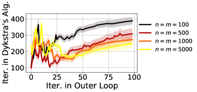
Figure 3: We consider samples of a mixture of 10 anisotropic Gaussians in resp. 10 and 15-D endowed with the squared Eucl. metric. The number of iterations of Dykstra’s algorithm required to reach a precision of $\delta=1e-3$ along the iterations of the Algo. 3 is not impacted significantly by varying $n$, the sample size.

Initialization. For a fair comparison with the entropic approach, we adapt the first lower bound of (Mémoli, 2011, Def. 6.1) to the entropic case to initialize it. In all experiments displaying time-accuracy tradeoffs, we report computation budget as number of operations. Accuracy is measured by evaluating the ground-truth energy $\mathcal{Q}_{A,B}$ (even in scenarios when the method uses a low rank approximation for $A,B$ at optimization time). We repeat all experiments 10 times on random resampling of the measures in all synthetic problems, to obtain error bars.

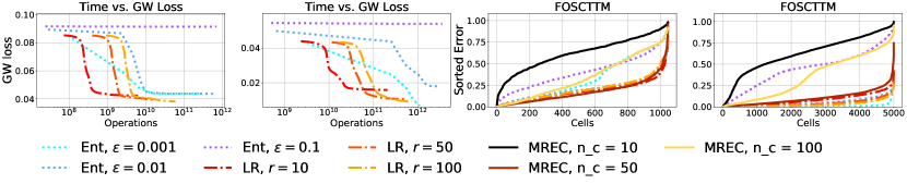
Figure 4: We consider both the SNAREseq dataset (left, middle-right) which consists in two point clouds of $n=m=1047$ samples in respectively 10-D and 19-D and the Splatter dataset (middle-left, right) composed of two point clouds of $n=m=5000$ samples in respectively 50-D and 500-D. The cost considered is the shortest-path distance of a $k-NN$ graph. We compare both the time-accuracy tradeoffs of our method with the Entropic-GW (left, middle-left) and the FOSCTTMs ranked in the increasing order of LR, Ent and MREC when varying their hyperparameters (middle-right, right). Because the coupling returned by MREC does not satisfy marginal constraints, we do not include it in left plots. Our method reaches similar accuracy while being order of magnitude faster than Ent even for a small rank $r=n/100$. We notice that the alignments obtained by our method are robust to the choice of $r$, with similar performance for all methods.

On the iterations of Dykstra’s Algorithm. In this experiment, we show that the number of iterations involved in the Dykstra’s Algorithm does not depends on $n$ the number of samples when applying Algo. 3. In Fig. 3, we consider samples of mixtures of (10 and 15) anisotropic Gaussians in resp. 10 and 15-D and report the number of iterations of the Dykstra’s Algorithm required to reach a precision $\delta=1e-3$ along the iterations of Algo. 3. We observe that the number of iterations in Dykstra does not depend on $n$ the number of samples considered. Note that for all the sample sizes considered, we need far fewer iterations (usually $\leq 25$) for the outer loop to converge: the plots show a larger $x$-axis than what is observed in practice.

Sensitity to $\gamma$ and $\alpha$.

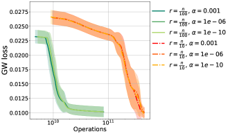
Figure 12: We consider $n=m=5000$ samples of mixtures of (2 and 3) Gaussians in resp. 5 and 10-D, endowed with the squared Euclidean metric, compared with Lin LR. The time/loss tradeoff illustrated in these plots show that our method is not impacted by step size $\alpha$ for both ranks $r=n/100$ and $n/10$.

We study how optimization parameters $\gamma$ and $\alpha$ impact results. We consider $n=m=1000$ samples drawn from two mixtures of (2 and 3) anisotropic Gaussians in respectively 5-D and 10-D (details in Appendix E.2). Fig. 9, reports the time vs. GW loss tradeoff of our method when varying $\gamma$, both for $r=n/100$ or $n/10$ illustrating its robustness to that choice. Fig. 12 in Appendix E.2 shows similar conclusions with respect to $\alpha$. Recall that $\alpha$ was only used to lower bound the weights of barycenter $g$, to ensure no collapse. In all other experiments, we always set $\gamma=100$ and $\alpha=10^{-10}$ for our methods, and only focus on rank $r$.

Effect of the rank.

We study the impact of rank $r$ on our method. We consider samples from two Gaussian mixtures, with respectively 10 and 20 centers in 10-D and 15-D and $n=m=5000$. We compute the GW cost obtained by Lin LR in the squared Euclidean setting as a function of $r$ the rank. We observe that the loss decreases as the rank increases until the rank $r$ reaches 20 (the largest number of clusters in our mixtures). Therefore, our method is able to capture the clustered structure of data (See Appendix E.3). In practice $r$ should be selected such that it corresponds to the number of clusters in the data.

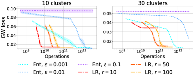
Figure 5: We sample $n=m=5000$ points from two anisotropic Gaussian blobs, respectively in 10 and 15-D, with either 10 or 30 clusters, endowed with the Euclidean distance. We compare our quadratic method LR with the cubic Entropic GW Ent, which requires instantiating matrices $A$ and $B$. We vary both $r$ (our method) and $\varepsilon$ (entropic). Our method obtains similar GW loss, while being orders of magnitude faster. Note the gap in performance between $r=10$ and $r=50$ when the input measures have 30 clusters: the GW loss decreases as the rank $r$ increases until it reaches the number of clusters in the data.

Synthetic low-rank problem.

We consider two anisotropic Gaussian blobs with the same number of blobs in respectively 10-D and 15-D. We constrain the distance between the centroids of the clusters to be larger than the dimension (see Appendix E.4 for illustrations). In Figures 5 and 6, when the underlying cost is the (not squared) Euclidean distance, our methods manage to consistently obtain similar GW loss that those obtained by entropic methods, using very low rank $r=n/100$, while being orders of magnitude faster. Fig. 7 explores the more favorable case where the underlying cost is the squared Euclidean distance, reaching similar conclusions.

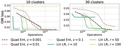
Figure 6: Same setting as Fig. 5, using a low-rank approximation of the Euclidean distance (see §3) to introduce our linear method Lin LR and compare it with Quad Ent. The rank of their factorizations is set to $d=d^{\prime}=100$. We vary $\varepsilon$ and rank $r$ to reach similar conclusions to those outlined in Fig. 5. Note also that both Lin LR and Quad Ent reach similar GW loss as those obtained by their full-rank counterparts, while being orders of magnitude faster.

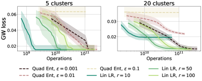
Figure 7: Setting as in Fig. 5, with $n=m=10000$ samples from anisotropic Gaussian blobs of 5 or 20 clusters, endowed with the squared Eucl. distance. We compare Lin LR and Quad Ent using exact factorizations of $A$ and $B$.

Large scale experiment.

In this experiment, we show that our method is able to compute an approximation of the GW cost in the large sample setting. In Fig. 8, we samples $n=m=1e5$ samples from the unit square in 2-D and we compare the time/loss tradeoff when varying the rank $r$. We show that our method is the only one able to approach the GW cost in such regimes.

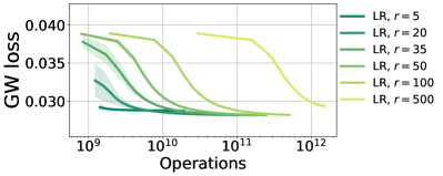
Figure 8: We sample $n=1e5$ points from the unit square in 2-D. The underlying cost considered is the squared Euclidean cost. In this regime, only Lin GW-LR can be computed. We plot the time/loss tradeoff when varying $r$.

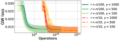
Figure 9: We consider two $n=m=1000$ samples of mixtures of (2 and 3) Gaussians in resp. 5 and 10-D, endowed with the squared Euclidean metric, compared with Lin LR. The time/loss tradeoff illustrated in these plots show that our method is only mildly impacted by step size $\gamma$ for both ranks $r=n/100$ and $n/10$.

Experiments on Single Cell Genomics Data.

We reproduce the single-cell alignment experiments introduced in (Demetci et al., 2020). The datasets consist in single-cell multi-omics data generated by co-assays, provided with a ground truth one–to-one correspondence, which can be used to benchmark GW strategies. The SNAREseq dataset (Chen et al., 2019), with $n=m=1047$ points in $\mathbb{R}^{19}$, describes a real-world experiment; the Splatter dataset (Zappia et al., 2017) with $n=m=5000$ points in $\mathbb{R}^{500}$ is synthetic. We use the pre-processing from (Demetci et al., 2020) to prepare intra-domain distance matrices $A$ and $B$ using a k-NN graph based on correlations, to compute shortest path distances. Note that in that case, one cannot obtain directly in linear time a low-rank factorization of $A$ and $B$ using (Bakshi and Woodruff, 2018; Indyk et al., 2019), since the shortest path distances need to be computed first. Therefore, we only use our quadratic approach LR and the cubic implementation of the entropic method Ent, along with MREC. In Fig. 4 we compare both the time/GW loss tradeoffs and the alignment performances through the “fraction of samples closer than the true match” (FOSCTTM) error introduced in (Liu et al., 2019). Note that we cannot compare the time-accuracy tradeoff of MREC with our method as the coupling obtained does not satisfy the marginal constraints. LR reaches similar loss, while being orders of magnitude faster than Ent, even for a very small rank $r=n/100$.

Experiment on BRAIN.

We reproduce the experiment proposed in (Blumberg et al., 2020). We consider the dataset introduced in (Lake et al., 2018) of single cells sampled from the human brain with eight different cell labels. The dataset contains two groups with different representations: one contains $n=34079$ cells represented by their genes expressions, while the second contains $m=27906$ cells represented by their DNA region accessibilities. We reuse the preprocessing in (Blumberg et al., 2020), by applying the method proposed in (Zheng et al., 2017) and available in Scanpy (Wolf et al., 2018) to the first group and a TF-IDF representation to the second one. A PCA is then performed on each group to reduce dimensions to 50, endowed with the squared Euclidean distance. These datasets are too large to be handled with entropic approaches, and show the potential of our linear approach Lin LR to handle larger scale problems. To compare Lin LR with MREC, we measure the accuracy of their matchings, as proposed in (Blumberg et al., 2020), by computing the fraction of points in the first group whose associated points under the matching given by the method share the same label in the second group. In Figure 10, we plot the accuracy against the rank (or the number of clusters in MREC) for both Lin LR and MREC. We also consider multiple versions of MREC by varying its entropic regularization parameter, $\varepsilon$, involved in the inner matching of the recursive method. Our method obtains consistently better accuracy than that obtained by MREC.

Discussion. While the factorization introduced in (Scetbon et al., 2021) held the promise to speed up classic OT, we show in this work that it delivers an even larger impact when applied to GW: indeed, the combination of low-rank Sinkhorn factorization with-low rank cost matrices is the only one, to our knowledge, that achieves linear time/memory complexity for the Gromov-Wasserstein problem. The GW problem is NP-hard, its optimal solution out of reach and approximate solutions can only be reached using an inductive bias. Here we propose to compute efficiently a coupling whose GW cost is low. By adding low-rank constraints, our goal is no longer to approach the optimal coupling, but rather to promote low-rank solutions among many that have a low GW cost. Our low-rank constraint obtains similar performance as the entropic regularization, the current default approach, while being much faster to compute. We show in experiments that low-rank couplings can reach low GW costs, and that they are directly useful in real-world tasks. Our approach has, however, a few limitations compared to the entropic one: setting $\gamma$, while not problematic in most of our experiments, could require a bit of tuning in order to obtain faster runs in challenging situations. Our assumptions to reach linearity, as discussed in §4 and 5 mostly rests on two important assumptions: the rank of distance matrices (the intrisic dimensionality of data points) must be such that $d,d^{\prime}$ are dominated by $n,m$ and that a small enough rank $r$ be able to capture the configuration of the input measures. Pending these constraints, which are valid in most relevant experimental setups we know of, we have demonstrated that our approach is versatile, remains faithful to the original GW formulation, and scales to sizes that are out of reach for the SoTA entropic solver.

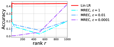
Figure 10: Using the BRAIN dataset (two point clouds of $n=34079$ and $m=27906$ samples in 50-D, endowed with squared Euclidean distance) we compare the GW loss against the rank (or the number of clusters) for both Lin LR and MREC for multiple choices of $\varepsilon$ in MREC. We show that our method is robust to the choice of the rank and obtains consistently better accuracy than MREC.

Supplementary material

Appendix A Proofs

A.1 Proof of Proposition 1

Proof.

Let $(Q,R,g)\in\mathcal{C}(a,b,r,\alpha)$, $P:=Q\operatorname{diag}(1/g)R^{T}$. Remarks that for all $i,j$,

$$\sqrt{\sum_{i^{\prime},j^{\prime}}|A_{i,i^{\prime}}-B_{j,j^{\prime}}|^{2}P_{i^{\prime},j^{\prime}}} \geq\left|\sqrt{\sum_{i^{\prime},j^{\prime}}|A_{i,i^{\prime}}|^{2}P_{i^{\prime},j^{\prime}}}-\sqrt{\sum_{i^{\prime},j^{\prime}}|B_{j,j^{\prime}}|^{2}P_{i^{\prime},j^{\prime}}}\right|$$

$$\geq|\sqrt{\tilde{x}_{i}}-\sqrt{\tilde{y}_{j}}|$$

Therefore we have

$$\sqrt{\sum_{i,i^{\prime},j,j^{\prime}}|A_{i,i^{\prime}}-B_{j,j^{\prime}}|^{2}P_{i^{\prime},j^{\prime}}P_{i,j}} =\sqrt{\sum_{i,j}\sum_{i^{\prime},j^{\prime}}|A_{i,i^{\prime}}-B_{j,j^{\prime}}|^{2}P_{i^{\prime},j^{\prime}}P_{i,j}}$$

$$\geq\sqrt{\sum_{i,j}|\sqrt{\tilde{x}_{i}}-\sqrt{\tilde{y}_{j}}|^{2}P_{i,j}}$$

Finally we obtain that

$$\sum_{i,i^{\prime},j,j^{\prime}}|A_{i,i^{\prime}}-B_{j,j^{\prime}}|^{2}P_{i^{\prime},j^{\prime}}P_{i,j}-\varepsilon H(Q,R,g) \geq\sum_{i,j}|\sqrt{\tilde{x}_{i}}-\sqrt{\tilde{y}_{j}}|^{2}P_{i,j}-\varepsilon H(Q,R,g)$$

and by taking the infimum over all $(Q,R,g)\in\mathcal{C}(a,b,r,\alpha)$, the results follows. ∎

A.2 Proof of Proposition 2

To show the result, we first need to recall some notions linked to the relative smoothness. Let $\mathcal{X}$ a closed convex subset in a Euclidean space $\mathbb{R}^{q}$. Given a convex function $H:\mathcal{X}\rightarrow\mathbb{R}$ continuously differentiable, one can define the Bregman divergence associated to $H$ as

$$D_{H}(x,z):=H(x)-H(z)-\langle\nabla H(z),x-z\rangle.$$

Let us now introduce the definition of the relative smoothness with respect the $H$.

Definition 1 (Relative smoothness.).

Let $L>0$ and $f$ continuously differentiable on $\mathcal{X}$. $f$ is said to be $L$-smooth relatively to $H$ if

$$f(y)\leq f(x)+\langle\nabla f(x),y-x\rangle+LD_{H}(y,x)$$

In [Scetbon et al., 2021], the authors show the following general result on the non-asymptotic stationary convergence of the mirror-descent scheme defined by the following recursion:

$$x_{k+1}=\operatorname*{argmin}_{x\in\mathcal{X}}\langle\nabla f(x_{k}),x\rangle+\frac{1}{\gamma_{k}}D_{h}(x,x_{k})$$

where $(\gamma_{k})$ a sequence of positive step-size.

Proposition 3 ([Scetbon et al., 2021]).

Let $N\geq 1$, $f$ continuously differentiable on $\mathcal{X}$ which is $L$-smooth relatively to $H$. By considering for all $k=1,\dots,N$, $\gamma_{k}=1/2L$, and by denoting $D_{0}=f(x_{0})-\min_{x\in\mathcal{X}}f(x)$, we have

$$\min_{0\leq k\leq N-1}\Delta_{k}\leq\frac{4LD_{0}}{N}.$$

where for all $k=1,\dots,N$

$$\Delta_{k}:=\frac{1}{\gamma_{k}^{2}}(D_{H}(x_{k},x_{k+1})+D_{H}(x_{k+1},x_{k})).$$

Let us now show that our objective function is relatively smooth with respect the the KL divergence [Lu et al., 2017, Zhang et al., 2020]. The result of Propostion 2 will then follow from Proposition 3. Here $\mathcal{X}=\mathcal{C}(a,b,r,\alpha)$, $H$ is the negative entropy defined as

$$H(Q,R,g):=\sum_{i,j}Q_{i,j}(\log(Q_{i,j})-1)+\sum_{i,j}R_{i,j}(\log(R_{i,j})-1)+\sum_{j}g_{j}(\log(g_{j})-1),$$

and let us define for all $(Q,R,g)\in\mathcal{C}(a,b,r,\alpha)$

$$F_{\varepsilon}(Q,R,g):=-2\langle AQ\operatorname{diag}(1/g)R^{T}B,Q\operatorname{diag}(1/g)R^{T}\rangle+\varepsilon H(Q,R,g)\;.$$

Let us now show the following proposition.

Proposition 4.

Let $\varepsilon\geq 0$, $\frac{1}{r}\geq\alpha>0$ and let us denote $L_{\varepsilon,\alpha}:=27(\|A\|_{2}\|B\|_{2}/\alpha^{4}+\varepsilon)$. Then for all $(Q_{1},R_{1},g_{1}),(Q_{2},R_{2},g_{2})\in\mathcal{C}(a,b,r,\alpha)$, we have

$$\|\nabla F_{\varepsilon}(Q_{1},R_{1},g_{1})-\nabla F_{\varepsilon}(Q_{2},R_{2},g_{2})\|_{2}\leq L_{\varepsilon,\alpha}\|H(Q_{1},R_{1},g_{1})-H(Q_{2},R_{2},g_{2})\|_{2}$$

Proof.

Let $(Q,R,g)\in\mathcal{C}(a,b,r,\alpha)$ and let us denote $P=Q\operatorname{diag}(1/g)R^{T}$. We first have that

$$\nabla F_{\varepsilon}(Q,R,g)=\left(\nabla_{Q}F_{\varepsilon}(Q,R,g),\nabla_{R}F_{\varepsilon}(Q,R,g),\nabla_{g}F_{\varepsilon}(Q,R,g)\right)$$

where

$$\nabla_{Q}F_{\varepsilon}(Q,R,g) :=-4APBR\operatorname{diag}(1/g)+\varepsilon\log Q$$

$$\nabla_{R}F_{\varepsilon}(Q,R,g) :=-4BP^{T}AQ\operatorname{diag}(1/g)+\varepsilon\log R$$

$$\nabla_{g}F_{\varepsilon}(Q,R,g) :=-4\mathcal{D}(Q^{T}APBR)/g^{2}+\varepsilon\log g$$

First remarks that

$$\|\nabla_{Q}F_{\varepsilon}(Q_{1},R_{1},g_{1})-\nabla_{Q}F_{\varepsilon}(Q_{2},R_{2},g_{2})\|_{2} \leq 4\|AP_{1}BR_{1}\operatorname{diag}(1/g_{1})-AP_{2}BR_{2}\operatorname{diag}(1/g_{2})\|_{2}$$

$$+\varepsilon\|\log Q_{1}-\log Q_{2}\|_{2}\;.$$

Moreover we have

$$AP_{1}BR_{1}\operatorname{diag}(1/g_{1})-AP_{2}BR_{2}\operatorname{diag}(1/g_{2})=A((P_{1}-P_{2})BR_{1}\operatorname{diag}(1/g_{1})+P_{2}B(R_{1}\operatorname{diag}(1/g_{1})-R_{2}\operatorname{diag}(1/g_{2}))$$

where

$$P_{1}-P_{2}=(Q_{1}-Q_{2})\operatorname{diag}(1/g_{1})R_{1}^{T}+Q_{2}(\operatorname{diag}(1/g_{1})R_{1}^{T}-\operatorname{diag}(1/g_{2})R_{2}^{T})$$

and

$$R_{1}\operatorname{diag}(1/g_{1})-R_{2}\operatorname{diag}(1/g_{2})=(R_{1}-R_{2})\operatorname{diag}(1/g_{1})+R_{2}(\operatorname{diag}(1/g_{1})-\operatorname{diag}(1/g_{2}))\;.$$

Moreover we have

$$\|AP_{1}BR_{1}\operatorname{diag}(1/g_{1})-AP_{2}BR_{2}\operatorname{diag}(1/g_{2})\|\leq\|A\|\|B\|\|P_{1}-P_{2}\|/\alpha+\|A\|\|B\|\|R_{1}\operatorname{diag}(1/g_{1})-R_{2}\operatorname{diag}(1/g_{2})\|$$

then remark that

$$\|P_{1}-P_{2}\|\leq\|Q_{1}-Q_{2}\|/\alpha+\|R_{1}\operatorname{diag}(1/g_{1})-R_{2}\operatorname{diag}(1/g_{2})\|$$

and

$$\|R_{1}\operatorname{diag}(1/g_{1})-R_{2}\operatorname{diag}(1/g_{2})\|\leq\|R_{1}-R_{2}\|/\alpha+\|1/g_{1}-1/g_{2}\|$$

from which follows that

$$\|AP_{1}BR_{1}\operatorname{diag}(1/g_{1})-AP_{2}BR_{2}\operatorname{diag}(1/g_{2})\|\leq \frac{\|A\|\|B\|}{\alpha}\left(\frac{\|Q_{1}-Q_{2}\|}{\alpha}+\frac{\|R_{1}-R_{2}\|}{\alpha}+\|1/g_{1}-1/g_{2}\|\right)$$

$$+\|A\|\|B\|\left(\frac{\|R_{1}-R_{2}\|}{\alpha}+\|1/g_{1}-1/g_{2}\|\right)\;.$$

As $Q\rightarrow H(Q)$ is 1-strongly convex w.r.t to the $\ell_{2}$-norm on $\Delta_{n\times r}$, we have

$$\|Q_{1}-Q_{2}\|_{2}^{2} \leq\langle\log Q_{1}-\log Q_{2},Q_{1}-Q_{2}\rangle$$

$$\leq\|\log Q_{1}-\log Q_{2}\|_{2}\|Q_{1}-Q_{2}\|_{2}$$

from which follows that

$$\|Q_{1}-Q_{2}\|_{2}\leq\|\log Q_{1}-\log Q_{2}\|_{2}.$$

Moreover we have

$$\|1/g_{1}-1/g_{2}\|_{2}\leq\frac{\|g_{1}-g_{2}\|_{2}}{\alpha^{2}}\leq\frac{\|\log g_{1}-\log g_{2}\|_{2}}{\alpha^{2}}$$

Then we obtain that

$$\|\nabla_{Q}F_{\varepsilon}(Q_{1},R_{1},g_{1})-\nabla_{Q}F_{\varepsilon}(Q_{2},R_{2},g_{2})\|_{2} \leq\left(\frac{4\|A\|\|B\|}{\alpha^{2}}+\varepsilon\right)\|\log Q_{1}-\log Q_{2}\|_{2}$$

$$+(1+1/\alpha)\frac{4\|A\|\|B\|}{\alpha}\|\log R_{1}-\log R_{2}\|_{2}$$

$$(1+1/\alpha)\frac{4\|A\|\|B\|}{\alpha^{2}}\|\log g_{1}-\log g_{2}\|_{2}$$

Similarly we obtain that Then we obtain that

$$\|\nabla_{R}F_{\varepsilon}(Q_{1},R_{1},g_{1})-\nabla_{R}F_{\varepsilon}(Q_{2},R_{2},g_{2})\|_{2} \leq\left(\frac{4\|A\|\|B\|}{\alpha^{2}}+\varepsilon\right)\|\log R_{1}-\log R_{2}\|_{2}$$

$$+(1+1/\alpha)\frac{4\|A\|\|B\|}{\alpha}\|\log Q_{1}-\log Q_{2}\|_{2}$$

$$(1+1/\alpha)\frac{4\|A\|\|B\|}{\alpha^{2}}\|\log g_{1}-\log g_{2}\|_{2}$$

Moreover we have

$$\|\nabla_{g}F_{\varepsilon}(Q_{1},R_{1},g_{1})-\nabla_{g}F_{\varepsilon}(Q_{2},R_{2},g_{2})\|_{2}\leq 4\|\mathcal{D}(Q_{1}^{T}AP_{1}BR_{1})/g_{1}^{2}-\mathcal{D}(Q_{2}^{T}AP_{2}BR_{2})/g_{2}^{2}\|$$

$$+\varepsilon\|\log g_{1}-\log g_{2}\|$$

and

$$\mathcal{D}(Q_{1}^{T}AP_{1}BR_{1})/g_{1}^{2}-\mathcal{D}(Q_{2}^{T}AP_{2}BR_{2})/g_{2}^{2}= (1/g_{1}^{2}-1/g_{2}^{2})\mathcal{D}(Q_{1}^{T}AP_{1}BR_{1})$$

$$+\frac{1}{g_{2}^{2}}(\mathcal{D}(Q_{1}^{T}AP_{1}BR_{1})-\mathcal{D}(Q_{2}^{T}AP_{2}BR_{2}));.$$

Note also that

$$\|(1/g_{1}^{2}-1/g_{2}^{2})\mathcal{D}(Q_{1}^{T}AP_{1}BR_{1})\|\leq\frac{2\|A\|\|B\|}{\alpha^{3}}\|\log g_{1}-\log g_{2}\|$$

and

$$Q_{1}^{T}AP_{1}BR_{1}-Q_{2}^{T}AP_{2}BR_{2} =(Q_{1}^{T}-Q_{2}^{T})AP_{1}BR_{1}+Q_{2}^{T}A(P_{1}BR_{1}-P_{2}BR_{2})$$

$$=(Q_{1}^{T}-Q_{2}^{T})AP_{1}BR_{1}+Q_{2}^{T}A((P_{1}-P_{2})BR_{1}+P_{2}B(R_{1}-R_{2}))$$

from which follows that

$$\|\frac{1}{g_{2}^{2}}(\mathcal{D}(Q_{1}^{T}AP_{1}BR_{1})-\mathcal{D}(Q_{2}^{T}AP_{2}BR_{2}))\|\leq\frac{\|A\|\|B\|}{\alpha^{2}}\left(\|\log Q_{1}-\log Q_{2}\|+\|\log R_{1}-\log R_{2}\|+\|P_{1}-P_{2}\|\right)$$

and we obtain that

$$\|\nabla_{g}F_{\varepsilon}(Q_{1},R_{1},g_{1})-\nabla_{g}F_{\varepsilon}(Q_{2},R_{2},g_{2})\|_{2} \leq\left(\frac{4\|A\|\|B\|}{\alpha^{2}}+\frac{1}{\alpha}\right)\|\log Q_{1}-\log Q_{2}\|$$

$$+\left(\frac{4\|A\|\|B\|}{\alpha^{2}}+\frac{1}{\alpha}\right)\|\log R_{1}-\log R_{2}\|$$

$$+\left(\frac{4\|A\|\|B\|}{\alpha^{4}}+\frac{8\|A\|\|B\|}{\alpha^{3}}+\varepsilon\right)\|\log g_{1}-\log g_{2}\|$$

Finally we have

$$\|\nabla F_{\varepsilon}(Q_{1},R_{1},g_{1})-\nabla F_{\varepsilon}(Q_{2},R_{2},g_{2})\|_{2}^{2} \leq 3\left[\left(\frac{4\|A\|\|B\|}{\alpha^{2}}+\varepsilon\right)^{2}+(1+1/\alpha)^{2}\frac{16\|A\|^{2}\|B\|^{2}}{\alpha^{2}}+\left(\frac{4\|A\|\|B\|}{\alpha^{2}}+\frac{1}{\alpha}\right)^{2}\right]$$

$$\left(\|\log Q_{1}-\log Q_{2}\|^{2}+\|\log R_{1}-\log R_{2}\|^{2}\right)$$

$$+3\left[2(1+1/\alpha)^{2}\frac{16\|A\|\|^{2}B\|^{2}}{\alpha^{4}}+\left(\frac{4\|A\|\|B\|}{\alpha^{4}}+\frac{8\|A\|\|B\|}{\alpha^{3}}+\varepsilon\right)^{2}\right]$$

$$\|\log g_{1}-\log g_{2}\|^{2}$$

from which we obtain that

$$\|\nabla F_{\varepsilon}(Q_{1},R_{1},g_{1})-\nabla F_{\varepsilon}(Q_{2},R_{2},g_{2})\|_{2}^{2} \leq L_{\varepsilon,\alpha}^{2}\left(\|\log Q_{1}-\log Q_{2}\|^{2}+\|\log R_{1}-\log R_{2}\|^{2}+\|\log g_{1}-\log g_{2}\|^{2}\right)$$

and the result follows. ∎

Appendix B Double Regularization Scheme

Another way to stabilize the method is by considering a double regularization scheme as proposed in [Scetbon et al., 2021] where in addition of constraining the nonnegative rank of the coupling, we regularize the objective by adding an entropic term in $(Q,R,g)$, which is to be understood as that of the values of the three respective entropies evaluated for each term.

$$\text{GW-LR}^{(r)}_{\varepsilon,\alpha}((a,A),(b,B)):=\min_{(Q,R,g)\in\mathcal{C}(a,b,r,\alpha)}\mathcal{E}_{A,B}(Q\operatorname{diag}(1/g)R^{T})-\varepsilon H((Q,R,g))\;.$$ (7)

Mirror Descent Scheme. We propose to use a MD scheme with respect to the KL divergence to approximate $\text{GW-LR}^{(r)}_{\varepsilon,\alpha}$ defined in (7). More precisely, for any $\varepsilon\geq 0$, the MD scheme leads for all $k\geq 0$ to the following updates which require solving a convex barycenter problem per step:

$$(Q_{k+1},R_{k+1},g_{k+1}):=\!\!\operatorname*{argmin}_{\zeta\in\mathcal{C}(a,b,r,\alpha)}\!\!\text{KL}(\zeta,K_{k})$$ (8)

where $(Q_{0},R_{0},g_{0})\in\mathcal{C}(a,b,r)$ is an initial point such that $Q_{0}>0$ and $R_{0}>0$, $P_{k}:=Q_{k}\operatorname{diag}(1/g_{k})R_{k}^{T}$, $K_{k}:=(K_{k}^{(1)},K_{k}^{(2)},K_{k}^{(3)})$, $K_{k}^{(1)}:=\exp(4\gamma AP_{k}BR_{k}\operatorname{diag}(1/g_{k})-(\gamma\varepsilon-1)\log(Q_{k}))$, $K_{k}^{(2)}:=\exp(4\gamma BP^{T}_{k}DQ_{k}\operatorname{diag}(1/g_{k})-(\gamma\varepsilon-1)\log(R_{k}))$, $K_{k}^{(3)}:=\exp(-4\gamma\omega_{k}/g_{k}^{2}-(\gamma\varepsilon-1)\log(g_{k}))$ with $[\omega_{k}]_{i}:=[Q_{k}^{T}AP_{k}BR_{k}]_{i,i}$ for all $i\in\{1,\dots,r\}$ and $\gamma$ is a positive step size. Solving (6) can be done efficiently thanks to the Dykstra’s Algorithm as showed in [Scetbon et al., 2021]. See Appendix D for more details.

Convergence of the mirror descent. Even if the objective (7) is not convex in $(Q,R,g)$, we obtain the non-asymptotic stationary convergence of the MD algorithm in this setting. For that purpose we consider the same convergence criterion as the one proposed in [Scetbon et al., 2021] to obtain non-asymptotic stationary convergence of the MD scheme defined as

$$\Delta_{\varepsilon,\alpha}(\xi,\gamma):=\frac{1}{\gamma^{2}}(\text{KL}(\xi,\mathcal{G}_{\varepsilon,\alpha}(\xi,\gamma))+\text{KL}(\mathcal{G}_{\varepsilon,\alpha}(\xi,\gamma),\xi))$$

where $\mathcal{G}_{\varepsilon,\alpha}(\xi,\gamma):=\operatorname*{argmin}_{\zeta\in\mathcal{C}(a,b,r,\alpha)}\{\langle\nabla\mathcal{E}_{A,B}(\xi),\zeta\rangle+\frac{1}{\gamma}\text{KL}(\zeta,\xi)\}.$ For any $1/r\geq\alpha>0$, we show in the following proposition the non-asymptotic stationary convergence of the MD scheme applied to the problem (7). See Appendix A for the proof.

Proposition 5.

Let $\varepsilon\geq 0$, $\frac{1}{r}\geq\alpha>0$ and $N\geq 1$. By denoting $L_{\varepsilon,\alpha}:=27(\|A\|_{2}\|B\|_{2}/\alpha^{4}+\varepsilon)$ and by considering a constant stepsize in the MD scheme (6) $\gamma=\frac{1}{2L_{\varepsilon,\alpha}}$, we obtain that

$$\min_{1\leq k\leq N}\Delta_{\varepsilon,\alpha}((Q_{k},R_{k},g_{k}),\gamma)\leq\frac{4L_{\varepsilon,\alpha}D_{0}}{N}.$$

where $D_{0}:=\mathcal{E}_{A,B}(Q_{0}\operatorname{diag}(1/g_{0}R_{0}^{T})-\text{{GW-LR}}^{(r)}((a,A),(b,B))$ is the distance of the initial value to the optimal one.

Appendix C Low-rank Approximation of Distance Matrices

Here we recall the algorithm used to perform a low-rank approximation of a distance matrix [Bakshi and Woodruff, 2018, Indyk et al., 2019]. We use the implementation of [Scetbon et al., 2021].

Inputs: $X,Y,r,\gamma$
Choose $i^{*}\in\{1,\dots,n\}$, and $j^{*}\{1,\dots,m\}$ uniformly at random.
For $i=1,\dots,n$, $p_{i}\leftarrow d(x_{i},y_{j}^{*})^{2}+d(x_{i}^{*},y_{j}^{*})^{2}+\frac{1}{m}\sum_{j=1}^{m}d(x_{i}^{*},y_{j})^{2}$.
Independently choose $i^{(1)},\dots,i^{(t)}$ according $(p_{1},\dots,p_{n})$.
$X^{(t)}\leftarrow[x_{i^{(1)}},\dots,x_{i^{(t)}}],~{}P^{(t)}\leftarrow[\sqrt{tp_{i^{(1)}}},\dots,\sqrt{tp_{i^{(t)}}}],~{}S\leftarrow d(X^{(t)},Y)/P^{(t)}$
Denote $S=[S^{(1)},\dots,S^{(m)}]$,
For $j=1,\dots,m$, $q_{j}\leftarrow\|S^{(j)}\|_{2}^{2}/\|S\|_{F}^{2}$
Independently choose $j^{(1)},\dots,j^{(t)}$ according $(q_{1},\dots,q_{m})$.
$S^{(t)}\leftarrow[S^{j^{(1)}},\dots,S^{j^{(t)}}],~{}Q^{(t)}\leftarrow[\sqrt{tq_{j^{(1)}}},\dots,\sqrt{tq_{j^{(t)}}}],~{}W\leftarrow S^{(t)}/Q^{(t)}$
$U_{1},D_{1},V_{1}\leftarrow\text{SVD}(W)$ (decreasing order of singular values).
$N\leftarrow[U_{1}{(1)},\dots,U_{1}^{(r)}],~{}N\leftarrow S^{T}N/\|W^{T}N\|_{F}$
Choose $j^{(1)},\dots,j^{(t)}$ uniformly at random in $\{1,\dots,m\}$.
$Y^{(t)}\leftarrow[y_{j^{(1)}},\dots,y_{j^{(t)}}],D^{(t)}\leftarrow d(X,Y^{(t)})/\sqrt{t}$.
$U_{2},D_{2},V_{2}=\text{SVD}(N^{T}N),~{}U_{2}\leftarrow U_{2}/D_{2},~{}N^{(t)}\leftarrow[(N^{T})^{(j^{(1)})},\dots,(N^{T})^{(j^{(t)})}],~{}B\leftarrow U_{2}^{T}N^{(t)}/\sqrt{t},~{}A\leftarrow(BB^{T})^{-1}$.
$Z\leftarrow AB(D^{(t)})^{T},~{}M\leftarrow Z^{T}U_{2}^{T}$
Result: $M,N$

Algorithm 4 $\text{LR-Distance}(X,Y,r,\gamma)$  [Bakshi and Woodruff, 2018, Indyk et al., 2019]

Appendix D Nonnegative Low-rank Factorization of the Couplings

In this section, we recall the algorithm presented in [Scetbon et al., 2021] to solve problem (6) where we denote $p_{1}:=a$ and $p_{2}:=b$.

Inputs: $K^{(1)},K^{(2)},\tilde{g}:=K^{(3)},p_{1},p_{2},\alpha,\delta,q^{(3)}_{1}=q^{(3)}_{2}=\mathbf{1}_{r},\forall i\in\{1,2\},~{}\tilde{v}^{(i)}=\mathbf{1}_{r},q^{(i)}=\mathbf{1}_{r}$
repeat

       $u^{(i)}\leftarrow p_{i}/K^{(i)}\tilde{v}^{(i)}~{}\forall i\in\{1,2\}$, $g\leftarrow\max(\alpha,\tilde{g}\odot q^{(3)}_{1}),~{}q^{(3)}_{1}\leftarrow(\tilde{g}\odot q^{(3)}_{1})/g,~{}\tilde{g}\leftarrow g$, $g\leftarrow(\tilde{g}\odot q^{(3)}_{2})^{1/3}\prod_{i=1}^{2}(v^{(i)}\odot q^{(i)}\odot(K^{(i)})^{T}u^{(i)})^{1/3}$, $v^{(i)}\leftarrow g/(K^{(i)})^{T}u^{(i)}~{}\forall i\in\{1,2\}$, $q^{(i)}\leftarrow(\tilde{v}^{(i)}\odot q^{(i)})/v^{(i)}~{}\forall i\in\{1,2\},~{}q^{(3)}_{2}\leftarrow(\tilde{g}\odot q^{(3)}_{2})/g$, $\tilde{v}^{(i)}\leftarrow v^{(i)}~{}\forall i\in\{1,2\},~{}\tilde{g}\leftarrow g$,

until $\sum_{i=1}^{2}\|u^{(i)}\odot K^{(i)}v^{(i)}-p_{i}\|_{1}<\delta$;

$Q\leftarrow\operatorname{diag}(u^{(1)})K^{(1)}\operatorname{diag}(v^{(1)})$
$R\leftarrow\operatorname{diag}(u^{(2)})K^{(2)}\operatorname{diag}(v^{(2)})$
Result: $Q,R,g$

Algorithm 5 $\text{LR-Dykstra}((K^{(i)})_{1\leq i\leq 3},p_{1},p_{2},\alpha,\delta)$  [Scetbon et al., 2021]

Appendix E Additional Experiements

E.1 Illustration

In Fig. 11, we show the time-accuracy tradeoffs of the two methods presented in Figure 2 on the same example. We see that our method, Lin GW-LR, manages to obtain similar accuracy as the one obtained by Quad Entropic-GW even when the rank $r=n/1000$ while being much faster with order of magnitude.

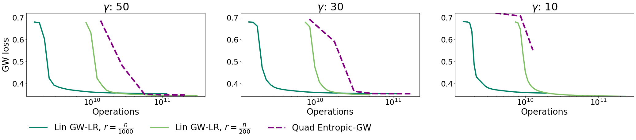
Figure 11: Here $n=m=10000$, and the ground cost considered is the squared Euclidean distance. Note that for in that case we have an exact low-rank factorization of the cost. Therefore we compare only Quad Entropic-GW and Lin GW-LR. We plot the time-accuracy tradeoff when varying $\gamma$ for multiple ranks $r$. $\varepsilon=1/\gamma$ for Quad Entropic-GW and $\varepsilon=0$ for Lin GW-LR.

E.2 Effect of $\gamma$ and $\alpha$

In Fig. 9 and 12, we consider two Gaussian mixture densities in respectively 5-D and 10-D where we generate randomly the mean and covariance matrice of each Gaussian density using the wishart distribution.

E.3 Effect of the Rank

In this experiment we compare two isotropic Gaussian blobs with respectively 10 and 20 centers in 10-D and 15-D and $n=m=5000$ samples. In Fig. 13, we show the two first coordinates of the dataset considered.

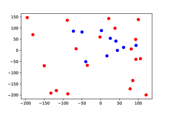
Figure 13: We consider two isotropic Gaussian blobs with respectively 10 and 20 centers in 10-D and 15-D and $n=m=5000$ samples and we plot their 2 first coordinates.

E.4 Low-rank Problem

In Fig. 5, 6 and 7, we consider two distributions in respectively 10-D and 15-D where the support is a concatenation of clusters of points. In Fig. 14, we show an illustration of the distributions considered in smaller dimensions.

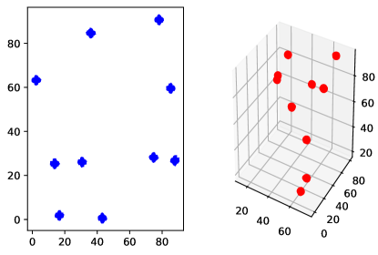
Figure 14: The source distribution and the target distribution live respectively in $\mathbb{R}^{2}$ and $\mathbb{R}^{3}$. Both distributions have the same number of samples $n=m=10000$, the same number of clusters which is set to be $10$ here, the same number of points in each cluster, and we force the distance between the centroids of the cluster to be larger than $\beta=10$ in each distribution.

E.5 Ground Truth Experiment

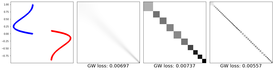
Figure 15: We compare the couplings obtained when the ground truth is the identity matrix in the same setting as in Figure 11. Here the comparison is done when $\gamma=250$. Left: illustration of the dataset considered. Middle left: we show the coupling as well as the GW loss obtained by Quad Entropic-GW. Middle right, right: we show the couplings and the GW losses obtained by Lin GW-LR when the rank is respectively $r=10$ and $r=100$.

In this experiment we aim at comparing the different methods when the optimal coupling solving the GW problem has a full rank. For that purpose we consider a certain shape in 2-D which corresponds to the support of the source distribution and we apply two isometric transformations to it, which are a rotation and a translation to obtain the support the target distribution. See Figure 15 (left) for an illustration of the dataset. Here we set $a$ and $b$ to be uniform distributions and the underlying cost is the squared Euclidean distance. Therefore the optimal coupling solution of the GW problem is the identity matrix and the GW loss must be 0. In Figure 16, we compare the time-accuracy tradeoffs, and we show that even in that case, our methods obtain a better time-accuracy tradeoffs for all $\gamma$. See also Figure 15 for a comparison of the couplings obtained by the different methods.

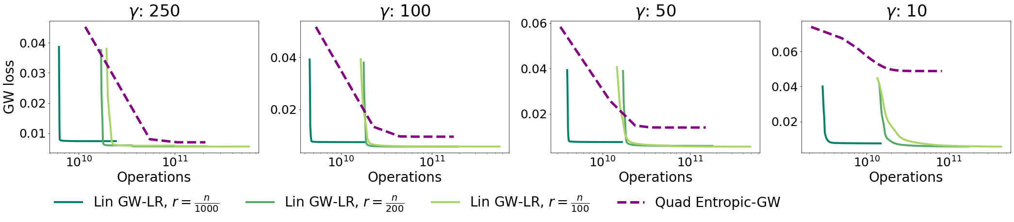
Figure 16: The ground truth here is the identity matrix and the true GW loss to achieve is 0. We set the number of samples to be $n=m=10000$. As we consider the squared Euclidean distance, only Quad Entropic-GW and Lin GW-LR are compared. We plot the time-accuracy tradeoff when varying $\gamma$ for multiple choices of rank $r$. $\varepsilon=1/\gamma$ for Quad Entropic-GW and $\varepsilon=0$ for Lin GW-LR.

References

- Altschuler et al. (2017) Jason Altschuler, Jonathan Weed, and Philippe Rigollet. Near-linear time approximation algorithms for optimal transport via sinkhorn iteration. arXiv preprint arXiv:1705.09634, 2017.
- Altschuler et al. (2018a) Jason Altschuler, Francis Bach, Alessandro Rudi, and Jonathan Niles-Weed. Massively scalable sinkhorn distances via the nyström method, 2018a.
- Altschuler et al. (2018b) Jason Altschuler, Francis Bach, Alessandro Rudi, and Jonathan Weed. Approximating the quadratic transportation metric in near-linear time. arXiv preprint arXiv:1810.10046, 2018b.
- Bakshi and Woodruff (2018) Ainesh Bakshi and David P. Woodruff. Sublinear time low-rank approximation of distance matrices, 2018.
- Blumberg et al. (2020) Andrew J Blumberg, Mathieu Carriere, Michael A Mandell, Raul Rabadan, and Soledad Villar. Mrec: a fast and versatile framework for aligning and matching point clouds with applications to single cell molecular data. arXiv preprint arXiv:2001.01666, 2020.
- Bunne et al. (2019) Charlotte Bunne, David Alvarez-Melis, Andreas Krause, and Stefanie Jegelka. Learning generative models across incomparable spaces. arXiv preprint arXiv:1905.05461, 2019.
- Burkard et al. (1998) Rainer E Burkard, Eranda Cela, Panos M Pardalos, and Leonidas S Pitsoulis. The quadratic assignment problem. In Handbook of combinatorial optimization, pages 1713–1809. Springer, 1998.
- Chapel et al. (2020) Laetitia Chapel, Mokhtar Alaya, and Gilles Gasso. Partial optimal transport with applications on positive-unlabeled learning. In Advances in Neural Information Processing Systems 33 (NeurIPS 2020), 2020.
- Chen et al. (2019) Song Chen, Blue B Lake, and Kun Zhang. High-throughput sequencing of the transcriptome and chromatin accessibility in the same cell. Nature biotechnology, 37(12):1452–1457, 2019.
- Chowdhury et al. (2021) Samir Chowdhury, David Miller, and Tom Needham. Quantized gromov-wasserstein. arXiv preprint arXiv:2104.02013, 2021.
- Cuturi (2013) Marco Cuturi. Sinkhorn distances: Lightspeed computation of optimal transport. In Advances in neural information processing systems, pages 2292–2300, 2013.
- Demetci et al. (2020) Pinar Demetci, Rebecca Santorella, Björn Sandstede, William Stafford Noble, and Ritambhara Singh. Gromov-wasserstein optimal transport to align single-cell multi-omics data. bioRxiv, 2020. doi: 10.1101/2020.04.28.066787.
- Dudley et al. (1966) Richard Mansfield Dudley et al. Weak convergence of probabilities on nonseparable metric spaces and empirical measures on euclidean spaces. Illinois Journal of Mathematics, 10(1):109–126, 1966.
- Ezuz et al. (2017) Danielle Ezuz, Justin Solomon, Vladimir G Kim, and Mirela Ben-Chen. Gwcnn: A metric alignment layer for deep shape analysis. In Computer Graphics Forum, volume 36, pages 49–57. Wiley Online Library, 2017.
- Forrow et al. (2019) Aden Forrow, Jan-Christian Hütter, Mor Nitzan, Philippe Rigollet, Geoffrey Schiebinger, and Jonathan Weed. Statistical optimal transport via factored couplings. In The 22nd International Conference on Artificial Intelligence and Statistics, pages 2454–2465. PMLR, 2019.
- Ghadimi et al. (2013) Saeed Ghadimi, Guanghui Lan, and Hongchao Zhang. Mini-batch stochastic approximation methods for nonconvex stochastic composite optimization, 2013.
- Gold and Rangarajan (1996) Steven Gold and Anand Rangarajan. Softassign versus softmax: Benchmarks in combinatorial optimization. Advances in neural information processing systems, pages 626–632, 1996.
- Indyk et al. (2019) Piotr Indyk, Ali Vakilian, Tal Wagner, and David Woodruff. Sample-optimal low-rank approximation of distance matrices, 2019.
- Konno (1976) Hiroshi Konno. Maximization of a convex quadratic function under linear constraints. Mathematical programming, 11(1):117–127, 1976.
- Lake et al. (2018) Blue B Lake, Song Chen, Brandon C Sos, Jean Fan, Gwendolyn E Kaeser, Yun C Yung, Thu E Duong, Derek Gao, Jerold Chun, Peter V Kharchenko, et al. Integrative single-cell analysis of transcriptional and epigenetic states in the human adult brain. Nature biotechnology, 36(1):70–80, 2018.
- Le et al. (2021) Tam Le, Nhat Ho, and Makoto Yamada. Flow-based alignment approaches for probability measures in different spaces. In International Conference on Artificial Intelligence and Statistics, pages 3934–3942. PMLR, 2021.
- Lin et al. (2019) Tianyi Lin, Nhat Ho, and Michael Jordan. On efficient optimal transport: An analysis of greedy and accelerated mirror descent algorithms. In International Conference on Machine Learning, pages 3982–3991. PMLR, 2019.
- Liu et al. (2019) Jie Liu, Yuanhao Huang, Ritambhara Singh, Jean-Philippe Vert, and William Stafford Noble. Jointly embedding multiple single-cell omics measurements. BioRxiv, page 644310, 2019.
- Lu et al. (2017) Haihao Lu, Robert M. Freund, and Yurii Nesterov. Relatively-smooth convex optimization by first-order methods, and applications, 2017.
- Mémoli (2011) Facundo Mémoli. Gromov–wasserstein distances and the metric approach to object matching. Foundations of computational mathematics, 11(4):417–487, 2011.
- Peyré et al. (2016) Gabriel Peyré, Marco Cuturi, and Justin Solomon. Gromov-wasserstein averaging of kernel and distance matrices. In International Conference on Machine Learning, pages 2664–2672, 2016.
- Peyré and Cuturi (2019) Gabriel Peyré and Marco Cuturi. Computational optimal transport. Foundations and Trends in Machine Learning, 11(5-6), 2019. ISSN 1935-8245.
- Sato et al. (2020) Ryoma Sato, Marco Cuturi, Makoto Yamada, and Hisashi Kashima. Fast and robust comparison of probability measures in heterogeneous spaces. arXiv preprint arXiv:2002.01615, 2020.
- Scetbon and Cuturi (2020) Meyer Scetbon and Marco Cuturi. Linear time sinkhorn divergences using positive features, 2020.
- Scetbon et al. (2021) Meyer Scetbon, Marco Cuturi, and Gabriel Peyré. Low-rank sinkhorn factorization, 2021.
- Sinkhorn (1964) Richard Sinkhorn. A relationship between arbitrary positive matrices and doubly stochastic matrices. Ann. Math. Statist., 35:876–879, 1964.
- Solomon et al. (2015) Justin Solomon, Fernando De Goes, Gabriel Peyré, Marco Cuturi, Adrian Butscher, Andy Nguyen, Tao Du, and Leonidas Guibas. Convolutional Wasserstein distances: efficient optimal transportation on geometric domains. ACM Transactions on Graphics, 34(4):66:1–66:11, 2015.
- Solomon et al. (2016) Justin Solomon, Gabriel Peyré, Vladimir G Kim, and Suvrit Sra. Entropic metric alignment for correspondence problems. ACM Transactions on Graphics (TOG), 35(4):1–13, 2016.
- Sturm (2012) Karl-Theodor Sturm. The space of spaces: curvature bounds and gradient flows on the space of metric measure spaces. arXiv preprint arXiv:1208.0434, 2012.
- Vayer et al. (2018) Titouan Vayer, Laetita Chapel, Rémi Flamary, Romain Tavenard, and Nicolas Courty. Fused gromov-wasserstein distance for structured objects: theoretical foundations and mathematical properties. arXiv preprint arXiv:1811.02834, 2018.
- Vayer et al. (2019) Titouan Vayer, Rémi Flamary, Romain Tavenard, Laetitia Chapel, and Nicolas Courty. Sliced gromov-wasserstein. arXiv preprint arXiv:1905.10124, 2019.
- Weed and Bach (2019) Jonathan Weed and Francis Bach. Sharp asymptotic and finite-sample rates of convergence of empirical measures in wasserstein distance. Bernoulli, 25(4A):2620–2648, 2019.
- Wolf et al. (2018) F Alexander Wolf, Philipp Angerer, and Fabian J Theis. Scanpy: large-scale single-cell gene expression data analysis. Genome biology, 19(1):1–5, 2018.
- Xu et al. (2019a) Hongteng Xu, Dixin Luo, and Lawrence Carin. Scalable gromov-wasserstein learning for graph partitioning and matching. arXiv preprint arXiv:1905.07645, 2019a.
- Xu et al. (2019b) Hongteng Xu, Dixin Luo, Hongyuan Zha, and Lawrence Carin Duke. Gromov-wasserstein learning for graph matching and node embedding. In International conference on machine learning, pages 6932–6941. PMLR, 2019b.
- Zappia et al. (2017) Luke Zappia, Belinda Phipson, and Alicia Oshlack. Splatter: simulation of single-cell rna sequencing data. bioRxiv, 2017. doi: 10.1101/133173.
- Zhang et al. (2020) Kelvin Shuangjian Zhang, Gabriel Peyré, Jalal Fadili, and Marcelo Pereyra. Wasserstein control of mirror langevin monte carlo, 2020.
- Zheng et al. (2017) Grace XY Zheng, Jessica M Terry, Phillip Belgrader, Paul Ryvkin, Zachary W Bent, Ryan Wilson, Solongo B Ziraldo, Tobias D Wheeler, Geoff P McDermott, Junjie Zhu, et al. Massively parallel digital transcriptional profiling of single cells. Nature communications, 8(1):1–12, 2017.