The regularization continuation method with an adaptive time step control for linearly constrained optimization problems

Abstract

This paper considers the regularization continuation method and the trust-region updating strategy for the optimization problem with linear equality constraints. The proposed method utilizes the linear conservation law of the regularization continuation method such that it does not need to compute the correction step for preserving the feasibility other than the previous continuation methods and the quasi-Newton updating formulas for the linearly constrained optimization problem. Moreover, the new method uses the special limited-memory Broyden-Fletcher-Goldfarb-Shanno (L-BFGS) formula as the preconditioning technique to improve its computational efficiency in the well-posed phase, and it uses the inverse of the regularized two-sided projection of the Lagrangian Hessian as the pre-conditioner to improve its robustness. Numerical results also show that the new method is more robust and faster than the traditional optimization method such as the alternating direction method of multipliers (ADMM), the sequential quadratic programming (SQP) method (the built-in subroutine fmincon.m of the MATLAB2020a environment), and the recent continuation method (Ptctr). The computational time of the new method is about 1/3 of that of SQP (fmincon.m). Finally, the global convergence analysis of the new method is also given.

1 Introduction

In this article, we consider the optimization problem with linear equality constraints as follows:

$$\min_{x\in\Re^{n}}\;f(x)$$

$$\text{subject to}\;\;Ax=b,$$ (1)

where $A\in\Re^{m\times n}$ is a matrix and $b\in\Re^{m}$ is a vector. This problem has many applications in engineering fields such as the visual-inertial navigation of an unmanned aerial vehicle maintaining the horizontal flight CMFO2009 ; LLS2021 , constrained sparse regression BF2010 , sparse signal recovery FS2009 ; VLLW2006 , image restoration and de-noising FB2010 ; NWY2010 ; ST2010 , the Dantzig selector LPZ2012 , and support vector machines FCG2010 . And there are many practical methods to solve it such as the sequential quadratic programming (SQP) method LJYY2019 ; NW1999 , the penalty function method FM1990 , feasible direction methods (see pp. 515-516, SY2006 ), and the alternating direction method of multipliers (ADMM BPCE2011 ).

For the constrained optimization problem (1), the continuation method AG2003 ; CKK2003 ; Goh2011 ; KLQCRW2008 ; Pan1992 ; Tanabe1980 is another method other than the traditional optimization method such as SQP, the penalty function method and ADMM. The advantage of the continuation method over the SQP method is that the continuation method is capable of finding many local optimal points of the non-convex optimization problem by following its trajectory, and it is even possible to find the global optimal solution BB1989 ; Schropp2000 ; Yamashita1980 . However, the computational efficiency of the classical continuation method is inferior to that of the traditional optimization method such as SQP. Recently, the reference LLS2021 gives a continuation method with the trusty time-stepping scheme (Ptctr) for the problem (1) and it is faster than SQP and the penalty method. In order to improve the computational efficiency and the robustness of the continuation method for the large-scale optimization problem further, we consider a special limited-memory Broyden-Fletcher-Goldfarb-Shanno (L-BFGS) updating formula Broyden1970 ; Fletcher1970 ; Goldfarb1970 ; Shanno1970 as the preconditioned technique in the well-posed phase and use the inverse of the regularized two-sided projection of the Lagrangian Hessian as the pre-conditioner in the ill-posed phase. Moreover, the new method utilizes the linear conservation law of the regularization method and it does not need to compute the correction step for preserving the feasibility other than the previous continuation method LLS2021 and the quasi-Newton method NW1999 ; SY2006 .

The rest of the paper is organized as follows. In section 2, we give the regularization continuation method with the switching preconditioned technique and the trust-region updating strategy for the linearly constrained optimization problem (1). In section 3, we analyze the global convergence of this new method. In section 4, we report some promising numerical results of the new method, in comparison to the traditional optimization method such as SQP (the built-in subroutine fmincon.m of the MATLAB2020a environment MATLAB ), the alternating direction method of multipliers (ADMM BPCE2011 , only for convex problems), and the recent continuation method (Ptctr LLS2021 ) for some large-scale problems. Finally, we give some discussions and conclusions in section 5.

2 The adaptive regularization continuation method

In this section, we give the regularization continuation method with the switching preconditioned technique and an adaptive time-step control based on the trust-region updating strategy CGT2000 for the linearly constrained optimization problem (1). Firstly, we consider the regularized projection Newton flow based on the KKT conditions of linearly constrained optimization problem. Then, we give the regularization continuation method with the trust-region updating strategy to follow this special ordinary differential equations (ODEs). The new method uses a special L-BFGS updating formula as the preconditioned technique to improve its computational efficiency in the well-posed phase, and it uses the inverse of the regularized two-sided projection of the Lagrangian Hessian as the pre-conditioner to improve its robustness in the ill-posed phase. Finally, we give a preprocessing method for the infeasible initial point.

2.1 The regularization projected Newton flow

For the linearly constrained optimization problem (1), its optimal solution $x^{\ast}$ needs to satisfy the Karush-Kuhn-Tucker conditions (p. 328, NW1999 ) as follows:

$$\nabla_{x}L(x,\,\lambda) =\nabla f(x)+A^{T}\lambda=0,$$ (2)

$$Ax-b =0,$$ (3)

where the Lagrangian function $L(x,\,\lambda)$ is defined by

$$L(x,\,\lambda)=f(x)+\lambda^{T}(Ax-b).$$ (4)

Similarly to the method of the negative gradient flow for the unconstrained optimization problem HM1996 , from the first-order necessary conditions (2)-(3), we construct a dynamical system of differential-algebraic equations for problem (1) CL2011 ; LL2010 ; Luo2012 ; LLW2013 ; Schropp2003 as follows:

$$\frac{dx}{dt}=-\nabla L_{x}(x,\,\lambda)=-\left(\nabla f(x)+A^{T}\lambda\right),$$ (5)

$$Ax-b=0.$$ (6)

By differentiating the algebraic constraint (6) with respect to $t$ and substituting it into the differential equation (5), we obtain

$$A\frac{dx}{dt}=-A\left(\nabla f(x)+A^{T}\lambda\right)=-A\nabla f(x)-AA^{T}\lambda=0.$$ (7)

If we assume that matrix $A$ has full row rank further, from equation (7), we obtain

$$\lambda=-\left(AA^{T}\right)^{-1}A\nabla f(x).$$ (8)

By substituting $\lambda$ of equation (8) into equation (5), we obtain the projected gradient flow Tanabe1980 for the constrained optimization problem (1) as follows:

$$\frac{dx}{dt}=-\left(I-A^{T}\left(AA^{T}\right)^{-1}A\right)\nabla f(x)=-Pg(x),$$ (9)

where $g(x)=\nabla f(x)$ and the projection matrix $P$ is defined by

$$P=I-A^{T}\left(AA^{T}\right)^{-1}A.$$ (10)

It is not difficult to verify $P^{2}=P$. That is to say, the projection matrix $P$ is symmetric and its eigenvalues are either 0 or 1. From Theorem 2.3.1 (see p. 73, GV2013 ), we know that its matrix 2-norm is

$$\|P\|=1.$$ (11)

We denote $P^{+}$ as the Moore-Penrose generalized inverse of the projection matrix $P$ (see p. 11, SY2006 ). Since the projection matrix $P$ is symmetric and $P^{2}=P$, it is not difficult to verify

$$P^{+}=P.$$ (12)

Actually, from equation (12), we have $PP^{+}P=P(P)P=P=P^{+}$, $P^{+}PP^{+}=P^{3}=P$, $\left(P^{+}P\right)^{T}=P^{+}P=P$ and $\left(PP^{+}\right)^{T}=PP^{+}=P$.

Furthermore, from equation (10), we have $AP=0$. We denote $\mathcal{N}(A)$ as the null space of $A$. Since the rank of $A$ is $m$, we know that the rank of $\mathcal{N}(A)$ equals $n-m$ and there are $n-m$ linearly independent vectors $x_{i}\,(i=1,\,\ldots,\,n-m)$ to satisfy $Ax_{i}=0\,(i=1,\,\ldots,\,n-m)$. From equation (10), we know that those $n-m$ linearly independent vectors $x_{i}\,(i=1,\,\ldots,\,n-m)$ satisfy $Px_{i}=x_{i}\,(i=1,\,\ldots,\,n-m)$. That is to say, the projection matrix $P$ has $n-m$ linearly independent eigenvectors associated with eigenvalue 1. Consequently, the rank of $P$ is $n-m$. By combining it with $AP=0$, we know that $P$ spans the null space of $A$.

Remark 1

If $x(t)$ is the solution of the ODE (9), it is not difficult to verify that $x(t)$ satisfies $A(dx/dt)=0$. That is to say, if the initial point $x_{0}$ satisfies $Ax_{0}=b$, the solution $x(t)$ of the projected gradient flow (9) also satisfies the feasibility $Ax(t)=b,\;\forall t\geq 0$. This linear conservation property is very useful when we construct a structure-preserving algorithm HLW2006 ; Shampine1998 ; Shampine1999 to follow the trajectory of the ODE (9) to obtain its steady-state solution $x^{\ast}$.

If we assume that $x(t)$ is the solution of the ODEs (9), by using the property $P^{2}=P$, we obtain

$$\frac{df(x)}{dt}=\left(\nabla f(x)\right)^{T}\frac{dx}{dt}=-(\nabla f(x))^{T}P\nabla f(x)=-g(x)^{T}P^{2}g(x)=-\|Pg(x)\|^{2}\leq 0.$$

That is to say, $f(x)$ is monotonically decreasing along the solution curve $x(t)$ of the dynamical system (9). Furthermore, the solution $x(t)$ converges to $x^{\ast}$ when $f(x)$ is lower bounded and $t$ tends to infinity HM1996 ; Schropp2000 ; Tanabe1980 , where $x^{\ast}$ satisfies the first-order Karush-Kuhn-Tucker conditions (2)-(3). Thus, we can follow the trajectory $x(t)$ of the ODE (9) to obtain its steady-state solution $x^{\ast}$, which is also one stationary point of the original optimization problem (1).

However, since the Jacobian $P\nabla^{2}f(x)$ of $Pg(x)$ is rank-deficient, we will confront the numerical difficulties when we use the explicit ODE method to follow the projected gradient flow (9) AP1998 ; BCP1996 ; BJ1998 . In order to mitigate the stiffness of the ODE (9), we use the generalized inverse $(P\nabla^{2}f(x)P)^{+}$ of the two-sided projection $P\nabla^{2}f(x)P$ of the Lagrangian Hessian $\nabla^{2}_{xx}L(x,\,\lambda)$ as the pre-conditioner for the ODE (9), which is used similarly to the system of nonlinear equations LXL2021 , the unconstrained optimization problem HM1996 ; LXLZ2021 ; LX2022 , the linear programming problem LY2021 and the underdetermined system of nonlinear equations LX2021 .

Firstly, we integrate the ODE (9) from zero to $t$, then we obtain

$$x(t)=x(t_{0})-\int_{0}^{t}Pg(x(\tau))d\tau=x(t_{0})-P\int_{0}^{t}g(x(\tau))d\tau.$$ (13)

We denote $z(t)=-\int_{0}^{t}g(x(\tau))d\tau$. Thus, from equation (13), we have

$$x(t)=x(t_{0})+Pz(t).$$ (14)

By substituting it into the ODE (9), we obtain

$$P\frac{dz(t)}{dt}=-Pg(x(t_{0})+Pz(t)).$$ (15)

Then, by using the generalized inverse $\left(P\nabla^{2}f(x(t_{0})+Pz(t))P\right)^{+}$ of the Jacobian matrix $P\nabla^{2}f(x(t_{0})+Pz(t))P$ as the pre-conditioner for the ODE (15), we have

$$P\frac{dz(t)}{dt}=-\left(P\nabla^{2}f(x(t_{0})+Pz(t))P\right)^{+}Pg(x(t_{0})+Pz(t)).$$ (16)

We reformulate equation (16) as

$$\left(P\nabla^{2}f(x(t_{0})+Pz(t))P\right)\frac{dPz(t)}{dt}=-Pg(x(t_{0})+Pz(t)),$$ (17)

where we use the property $P^{2}=P$. We let $x(t)=Pz(t)+x(t_{0})$ and substitute it into equation (17). Then, we obtain the projected Newton flow for problem (1) as follows:

$$\left(P\nabla^{2}f(x)P\right)\frac{dx(t)}{dt}=-Pg(x).$$ (18)

Although the projected Newton flow (18) mitigates the stiffness of the ODE such that we can adopt the explicit ODE method to integrate it on the infinite interval, there are two disadvantages yet. One is that the two-side projection $P\nabla^{2}f(x)P$ may be not positive semi-definite. Consequently, it can not ensure that the objective function $f(x)$ is monotonically decreasing along the solution $x(t)$ of the ODE (18). The other is that the solution $x(t)$ of the ODE (18) may not satisfy the linear conservation law $Adx(t)/dt=0$. In order to overcome these two disadvantages, we use the similar regularization technique of solving the ill-posed problem Hansen1994 ; TA1977 for the projected Newton flow (18) as follows:

$$\left(\sigma(x)I+P\nabla^{2}f(x)P\right)\frac{dx(t)}{dt}=-Pg(x),$$ (19)

where the regularization parameter $\sigma(x)$ satisfies $\sigma(x)+\mu_{min}\left(P\nabla^{2}f(x)P\right)\geq\sigma_{min}>0$. Here, $\mu_{min}(B)$ represents the smallest eigenvalue of matrix $B$.

Remark 2

If we assume that $x(t)$ is the solution of the ODE (19), from the property $AP=0$, we have

$$A\left(\sigma(x)I+P\nabla^{2}f(x)P\right)\frac{dx(t)}{dt}=-APg(x)=0.$$

Consequently, we obtain $A\sigma(x)dx(t)/dt=0$. By integrating it, we obtain $Ax(t)=Ax(t_{0})=b$. That is to say, the solution $x(t)$ of the ODE (19) satisfies the linear conservation law $Ax=b$.

Remark 3

From the property $P^{2}=P$ and the ODE (19), we have

$$\left(\sigma(x)P+P\nabla^{2}f(x)P\right)\frac{dx(t)}{dt}=-Pg(x).$$ (20)

By subtracting equation (20) from equation (19), we obtain

$$\sigma(x)P\frac{dx(t)}{dt}-\sigma(x)\frac{dx(t)}{dt}=0.$$

Namely, when $x(t)$ is the solution of (19), it satisfies

$$P\frac{dx(t)}{dt}=\frac{dx(t)}{dt}.$$ (21)

Consequently, from equations (19), (21) and $\sigma(x)+\lambda_{min}\left(P\nabla^{2}f(x)P\right)\geq\sigma_{min}>0$, we obtain

$$\frac{df(x(t))}{dt}=(\nabla f(x))^{T}\frac{dx(t)}{dt}=(\nabla f(x))^{T}P\frac{dx(t)}{dt}=(Pg(x))^{T}\frac{dx(t)}{dt}$$

$$\hskip 5.69054pt=-(Pg(x))^{T}\left(\sigma(x)I+P^{T}\nabla^{2}f(x)P\right)^{-1}(Pg(x))\leq 0.$$

That is to say, $f(x)$ is monotonically decreasing along the solution $x(t)$ of the ODE (19). Furthermore, the solution $x(t)$ converges to $x^{\ast}$ when $f(x)$ is lower bounded and $\|P\nabla^{2}f(x)P\|\leq M$ HM1996 ; LQQ2004 ; Schropp2000 ; Tanabe1980 , where $M$ is a positive constant and $x^{\ast}$ is the stationary point of the regularized projection Newton flow (19). Thus, we can follow the trajectory $x(t)$ of the ODE (19) to obtain its stationary point $x^{\ast}$.

2.2 The regularization continuation method

The solution curve $x(t)$ of the ODE (19) may not be efficiently solved by the general ODE method such as backward differentiation formulas (BDFs, the subroutine ode15s.m of the MATLAB R2020a environment) AP1998 ; BCP1996 ; BJ1998 ; JT1995 . Thus, we need to construct the particular method for this problem. We apply the first-order explicit Euler method SGT2003 to the ODE (19), then we obtain the regularized projection Newton method:

$$\left(\sigma_{k}I+P\nabla^{2}f(x_{k})P\right)d_{k}=-Pg(x_{k}),$$ (22)

$$\hskip 5.69054ptx_{k+1}=x_{k}+\alpha_{k}d_{k},$$ (23)

where $\alpha_{k}$ is the time step. When $\alpha_{k}=1$, the regularized projection Newton method (22)-(23) equals the Levenberg-Marquardt method Levenberg1944 ; LLT2007 ; LLS2021 ; Marquardt1963 .

Since the time step $\alpha_{k}$ of the regularized projection Newton method (22)-(23) is restricted by the numerical stability SGT2003 . That is to say, for the linear test equation $dx/dt=-\lambda x$, its time step $\alpha_{k}$ is restricted by the stable region $|1-\alpha_{k}{\lambda}/(\sigma_{k}+\lambda)|\leq 1$. Therefore, the large time step can not be adopted in the steady-state phase. In order to avoid this disadvantage, similarly to the processing technique of the nonlinear equations LXL2021 ; LY2021 ; LX2021 and the unconstrained optimization problem LXLZ2021 ; LX2022 , we replace $\alpha_{k}$ with $\Delta t_{k}/(1+\Delta t_{k})$ in equation (23) and let $\sigma_{k}=\sigma_{0}/\Delta t_{k}$ in equation (22). Then, we obtain the regularization continuation method:

$$B_{k}d_{k}=-Pg(x_{k}),\;s_{k}=\frac{\Delta t_{k}}{1+\Delta t_{k}}d_{k},$$ (24)

$$\hskip 5.69054ptx_{k+1}=x_{k}+s_{k},$$ (25)

where $\Delta t_{k}$ is the time step and $B_{k}=\left((\sigma_{0}/\Delta t_{k})I+P\nabla^{2}f(x_{k})P\right)$ or its quasi-Newton approximation.

Remark 4

The time step $\Delta t_{k}$ of the regularization continuation method (24)-(25) is not restricted by the numerical stability. Therefore, the large time step $\Delta t_{k}$ can be adopted in the steady-state phase such that the regularization continuation method (24)-(25) mimics the projected Newton method near the stationary point $x^{\ast}$ and it has the fast convergence rate. The most of all, the new step $\alpha_{k}=\Delta t_{k}/(\Delta t_{k}+1)$ is favourable to adopt the trust-region updating strategy to adjust the time step $\Delta t_{k}$ such that the regularization continuation method (24)-(25) accurately follows the trajectory of the regularization flow (19) in the transient-state phase and achieves the fast convergence rate near its stationary point $x^{\ast}$.

When $B_{k}$ is updated by the BFGS quasi-Newton formula Broyden1970 ; BNY1987 ; Fletcher1970 ; Goldfarb1970 ; Shanno1970 as follows

$$B_{k+1}=B_{k}+\frac{y_{k}y_{k}^{T}}{y_{k}^{T}s_{k}}-\frac{B_{k}s_{k}s_{k}^{T}B_{k}}{s_{k}^{T}B_{k}s_{k}},\;B_{0}=I,$$ (26)

where $y_{k}=Pg(x_{k+1})-Pg(x_{k}),\;s_{k}=x_{k+1}-x_{k}$, there is an invariance for the transformation matrix $P$ and we state it as the following lemma 1.

Lemma 1

Assume that $B_{k}$ is updated by the BFGS quasi-Newton formula (26) and $s_{k}$ is solved by equation (24), then we have $P(B_{k}-I)=B_{k}-I$ and $Ps_{k}=s_{k}$ for $k=0,\,1,\,2,\,\ldots$.

Proof.  We prove this property by induction. When $k=0$, from $P^{2}=P$, we have $P(B_{0}-I)=0=B_{0}-I$ and $Ps_{0}=s_{0}$. We assume that $P(B_{l}-I)=B_{l}-I$ and $Ps_{l}=s_{l}$ when $k=l$. Then, when $k=l+1$, from $P^{2}=P$, $Py_{l}=P(Pg(x_{l+1})-Pg(x_{l}))=y_{l}$ and equation (26), we have

$$PB_{l+1} =PB_{l}+\frac{Py_{l}y_{l}^{T}}{y_{l}^{T}s_{l}}-\frac{PB_{l}s_{l}s_{l}^{T}B_{l}}{s_{l}^{T}B_{l}s_{l}}$$

$$=P+B_{l}-I+\frac{y_{l}y_{l}^{T}}{y_{l}^{T}s_{l}}-\frac{(P+B_{l}-I)s_{l}s_{l}^{T}B_{l}}{s_{l}^{T}B_{l}s_{l}}$$

$$=P-I+B_{l}+\frac{y_{l}y_{l}^{T}}{y_{l}^{T}s_{l}}-\frac{B_{l}s_{l}^{T}s_{l}B_{l}}{s_{l}^{T}B_{l}s_{l}}=P-I+B_{l+1}.$$ (27)

Consequently, we obtain $P(B_{l+1}-I)=B_{l+1}-I$.

From equation (24) and equation (27), we have

$$PB_{l+1}d_{l+1}=P(B_{l+1}d_{l+1})=-P(Pg(x_{l+1}))=-Pg(x_{l+1})=B_{l+1}d_{l+1},$$ (28)

$$PB_{l+1}d_{l+1}=(PB_{l+1})d_{l+1}=(P+B_{l+1}-I)d_{l+1}.$$ (29)

Consequently, from equations (28)-(29), we have $Pd_{l+1}=d_{l+1}$. By combining it with equation (24), we obtain $Ps_{l+1}=s_{l+1}$. Therefore, we know that the conclusion is true by induction. $\quad\square$

Remark 5

From equations (24)-(25), Lemma 1 and the property $AP=0$, it is not difficult to verify $As_{k}=0$. Thus, if the initial point $x_{0}$ is feasible, i.e. $Ax_{0}=b$, $x_{k}$ also satisfies the linear constraint $Ax_{k}=b$. That is to say, the regularization continuation method (24)-(25) satisfies the linear conservation law such that it does not need to compute the correction step for preserving the linear feasibility other than the previous continuation method and the quasi-Newton formula LLS2021 for the linearly constrained optimization problem (1).

2.3 The adaptive step control

Another issue is how to adaptively adjust the time step $\Delta t_{k}$ at every iteration. We borrow the adjustment technique of the trust-region radius from the trust-region method due to its robustness and its fast convergence rate CGT2000 ; Yuan2015 . According to the linear conservation law of the regularization continuation method (24)-(25), $x_{k+1}$ will preserve the feasibility when $Ax_{k}=b$. That is to say, $x_{k+1}$ satisfies $Ax_{k+1}=b$. Therefore, we use the objective function $f(x)$ instead of the nonsmooth penalty function $f(x)+\sigma\|Ax-b\|$ as the merit function. Similarly to the stepping-time scheme of the ODE method for the unconstrained optimization problem Higham1999 ; LLT2007 ; LLS2021 ; LXLZ2021 , we also need to construct a local approximation model of $f(x)$ around $x_{k}$. Here, we adopt the following quadratic function as its approximation model:

$$q_{k}(s)=f(x_{k})+s^{T}g_{k}+\frac{1}{2}s^{T}B_{k}s,$$ (30)

where $g_{k}=\nabla f(x_{k})$ and $B_{k}=(\sigma_{0}/{\Delta t_{k}})I+P\nabla^{2}f(x_{k})P$ or its quasi-Newton approximation.

In order to save the computational time, from the regularization continuation method (24)-(25), we simplify the quadratic model $q_{k}(s_{k})-q(0)$ as follows:

$$m_{k}(s_{k})=g_{k}^{T}s_{k}-\frac{0.5\Delta t_{k}}{1+\Delta t_{k}}g_{k}^{T}s_{k}=\frac{1+0.5\Delta t_{k}}{1+\Delta t_{k}}g_{k}^{T}s_{k}\approx q_{k}(s_{k})-q_{k}(0).$$ (31)

We enlarge or reduce the time step $\Delta t_{k}$ at every iteration according to the following ratio:

$$\rho_{k}=\frac{f(x_{k})-f(x_{k}+s_{k})}{m_{k}(0)-m_{k}(s_{k})}.$$ (32)

A particular adjustment strategy is given as follows:

$$\Delta t_{k+1}=\begin{cases}\gamma_{1}\Delta t_{k},&{\text{if}\hskip 2.84526pt0\leq\left|1-\rho_{k}\right|\leq\eta_{1},}\\ \Delta t_{k},&{\text{else if}\hskip 2.84526pt\eta_{1}<\left|1-\rho_{k}\right|<\eta_{2},}\\ \gamma_{2}\Delta t_{k},&{\text{others},}\end{cases}$$ (33)

where the constants are selected as $\eta_{1}=0.25,\;\gamma_{1}=2,\;\eta_{2}=0.75,\;\gamma_{2}=0.5$ according to our numerical experiments. We accept the trial step $s_{k}$ and let $x_{k+1}=x_{k}+s_{k}$, when $\rho_{k}\geq\eta_{a}$ and the approximation model $m_{k}(0)-m_{k}(s_{k})$ satisfies the Armijo sufficient descent condition:

$$m_{k}(0)-m_{k}(s_{k})\geq\eta_{m}\|s_{k}\|\|p_{g_{k}}\|,$$ (34)

where $\eta_{a}$ and $\eta_{m}$ are the small positive constants such as $\eta_{a}=\eta_{m}=1.0\times 10^{-6}$. Otherwise, we discard it and let $x_{k+1}=x_{k}$.

Remark 6

This new time-stepping scheme based on the trust-region updating strategy has some advantages, in comparison to the traditional line search strategy Luo2005 . If we use the line search strategy and the damped projected Newton method (22)-(23) to solve the projected Newton flow (19), in order to achieve the fast convergence rate in the steady-state phase, the time step $\alpha_{k}$ of the damped projected Newton method is tried from 1 and reduced by half with many times at every iteration. Since the linear model $f(x_{k})+g_{k}^{T}s_{k}$ may not approximate $f(x_{k}+s_{k})$ well in the transient-state phase, the time step $\alpha_{k}$ will be small. Consequently, the line search strategy consumes the unnecessary trial steps in the transient-state phase. However, the selection scheme of the time step based on the trust-region strategy (32)-(33) can overcome this shortcoming.

2.4 The switching preconditioned technique

For the large-scale problem, the numerical evaluation of the two-sided projection $P\nabla^{2}f(x_{k})P$ of the Lagrangian Hessian $\nabla^{2}_{xx}L(x,\,\lambda)$ consumes much time. In order to overcome this shortcoming, in the well-posed phase, we use the limited-memory BFGS quasi-Newton formula (see Broyden1970 ; Fletcher1970 ; Goldfarb1970 ; Mascarenhas2004 ; Shanno1970 or pp. 222-230, NW1999 ) to approximate the regularized two-sided projection $\left(\frac{\sigma_{0}}{\Delta t_{k}}I+P\nabla^{2}f(x_{k})P\right)$ of the regularization continuation method (24)-(25).

Recently, Ullah, Sabi’u and Shah USS2020 give an efficient L-BFGS updating formula for the system of monotone nonlinear equations. Furthermore, the reference LXLZ2021 also tests its efficiency for some unconstrained optimization problems. Therefore, we adopt the L-BFGS updating formula to approximate $\left(\frac{\sigma_{0}}{\Delta t_{k}}I+P\nabla^{2}f(x_{k})P\right)$ in the well-posed phase via slightly revising it as

$$B_{k+1}=\begin{cases}I-\frac{s_{k}s_{k}^{T}}{s_{k}^{T}s_{k}}+\frac{y_{k}y_{k}^{T}}{y_{k}^{T}y_{k}},\;\text{if}\;\left|s_{k}^{T}y_{k}\right|>\theta\|s_{k}\|^{2},\\ I,\;\text{otherwise},\end{cases}$$ (35)

where $s_{k}=x_{k+1}-x_{k},\;y_{k}=P\nabla f(x_{k+1})-P\nabla f(x_{k})$ and $\theta$ is a small positive constant such as $\theta=10^{-6}$.

By using the Sherman-Morrison-Woodburg formula (p. 17, SY2006 ), from equation (35), when $\left|y_{k}^{T}s_{k}\right|>\theta\|s_{k}\|^{2}$, we obtain the inverse of $B_{k+1}$ as follows:

$$B_{k+1}^{-1}=I-\frac{y_{k}s_{k}^{T}+s_{k}y_{k}^{T}}{y_{k}^{T}s_{k}}+2\frac{y_{k}^{T}y_{k}}{(y_{k}^{T}s_{k})^{2}}s_{k}s_{k}^{T}.$$ (36)

The initial matrix $B_{0}$ can be simply selected as an identity matrix. From equation (36), it is not difficult to verify

$$B_{k+1}s_{k}=\frac{y_{k}^{T}s_{k}}{y_{k}^{T}y_{k}}y_{k}.$$

That is to say, $B_{k+1}$ satisfies the scaling quasi-Newton property.

The L-BFGS updating formula (35) has some nice properties such as the symmetric positive definite property and the positive lower bound of its eigenvalues.

Lemma 2

When $\left|s_{k}^{T}y_{k}\right|>\theta\|s_{k}\|^{2}$, $B_{k+1}$ is symmetric positive definite and its eigenvalues are greater than $\left(\theta^{2}\|s_{k}\|^{2}\right)/\left(2\|y_{k}\|^{2}\right)$ and less than 2. Consequently, when $\left|s_{k}^{T}y_{k}\right|>\theta\|s_{k}\|^{2}$, the eigenvalues of $B_{k+1}^{-1}$ are greater than ${1}/{2}$ and less than $\frac{2\|y_{k}\|^{2}}{\theta^{2}\|s_{k}\|^{2}}$.

Proof.  (i) For any nonzero vector $z\in\Re^{n}$, from equation (35), we have

$$z^{T}B_{k+1}z=\|z\|^{2}-\frac{\left(z^{T}s_{k}\right)^{2}}{\|s_{k}\|^{2}}+\frac{\left(z^{T}y_{k}\right)^{2}}{\|y_{k}\|^{2}}\geq\frac{\left(z^{T}y_{k}\right)^{2}}{\|y_{k}\|^{2}}\geq 0.$$ (37)

In the first inequality of equation (37), we use the Cauchy-Schwartz inequality $\|z^{T}s_{k}\|\leq\|z\|\|s_{k}\|$ and its equality holds if only if $z=ts_{k}$. Therefore, $B_{k+1}$ is symmetric positive semi-definite. When $z=ts_{k}$, since $s_{k}^{T}y_{k}\neq 0$, from equation (37), we have $z^{T}B_{k+1}z=t^{2}{\left(s_{k}^{T}y_{k}\right)^{2}}/{\|y_{k}\|^{2}}>0$. Consequently, $B_{k+1}$ is symmetric positive definite when $s_{k}^{T}y_{k}\neq 0$.

(ii) It is not difficult to know that there exist at least $(n-2)$ linearly independent vectors $z_{1},\,z_{2},\,\ldots,\,z_{n-2}$ to satisfy $s_{k}^{T}z_{i}=0,\,y_{k}^{T}z_{i}=0\,(i=1:(n-2))$. That is to say, matrix $B_{k+1}$ defined by equation (35) has at least $(n-2)$ linearly independent eigenvectors associated with eigenvalue 1. We denote the other two eigenvalues of $B_{k+1}$ as $\mu_{i}^{k+1}\,(i=1:2)$ and set $\text{tr}(C)=\sum_{i=1}^{n}c_{ii},\,C\in\Re^{n\times n}$. Then, we have $\text{tr}(B_{k+1})=\mu_{1}^{k+1}+\mu_{2}^{k+1}+(n-2)$. By substituting it into equation (35), we obtain

$$\mu_{1}^{k+1}+\mu_{2}^{k+1}=\text{tr}(B_{k+1})-(n-2)$$

$$\hskip 5.69054pt=\text{tr}(I)-\text{tr}\left(\frac{s_{k}s_{k}^{T}}{s_{k}^{T}s_{k}}\right)+\text{tr}\left(\frac{y_{k}y_{k}^{T}}{y_{k}^{T}y_{k}}\right)-(n-2)=2,$$ (38)

where we use the property $\text{tr}\left(AB^{T}\right)=\text{tr}\left(B^{T}A\right)$ of matrices $A,\,B\in\Re^{m\times n}$. Since matrix $B_{k+1}$ is symmetric positive definite, we know that its eigenvalues are greater than 0, namely $\mu_{i}^{k+1}>0\,(i=1,\,2)$. By substituting it into equation (38), we obtain

$$0<\mu_{i}^{k+1}<\mu_{1}^{k+1}+\mu_{2}^{k+1}=2,\;i=1,\,2.$$ (39)

Furthermore, the symmetric matrix $B_{k+1}$ has a multiple eigenvalue 1 associated with $(n-2)$ linearly independent eigenvectors. Therefore, by combining it with equation (39), we know that the eigenvalues of matrix $B_{k+1}$ are less than 2.

We denote $\mu_{i}^{k+1}\,(i=1:n)$ as the eigenvalues of $B_{k+1}$. Then, we have $\mu_{i}^{k+1}=1\,(i=3:n)$. By using the property $\det(B_{k+1})=\prod_{i=1}^{n}\mu_{i}^{k+1}=\mu_{1}^{k+1}\mu_{2}^{k+1}$, from equation (35), we obtain

$$\mu_{1}^{k+1}\mu_{2}^{k+1}=\det(B_{k+1})=\det\left(\left(I+\frac{y_{k}y_{k}^{T}}{y_{k}^{T}y_{k}}\right)\left(I-\left(I+\frac{y_{k}y_{k}^{T}}{y_{k}^{T}y_{k}}\right)^{-1}s_{k}\frac{s_{k}^{T}}{s_{k}^{T}s_{k}}\right)\right)$$

$$\hskip 5.69054pt=\det\left(I+\frac{y_{k}y_{k}^{T}}{y_{k}^{T}y_{k}}\right)\det\left(I-\left(I+\frac{y_{k}y_{k}^{T}}{y_{k}^{T}y_{k}}\right)^{-1}s_{k}\frac{s_{k}^{T}}{s_{k}^{T}s_{k}}\right)$$

$$\hskip 5.69054pt=2\left(1-\frac{1}{\|s_{k}\|^{2}}s_{k}^{T}\left(I+\frac{y_{k}y_{k}^{T}}{y_{k}^{T}y_{k}}\right)^{-1}s_{k}\right)$$

$$\hskip 5.69054pt=2\left(1-\frac{1}{\|s_{k}\|^{2}}s_{k}^{T}\left(I-\frac{y_{k}y_{k}^{T}}{2y_{k}^{T}y_{k}}\right)s_{k}\right)=\frac{\left(s_{k}^{T}y_{k}\right)^{2}}{\left(y_{k}^{T}y_{k}\right)\left(s_{k}^{T}s_{k}\right)}.$$ (40)

From equation (39), we know $0<\mu_{i}^{k}<2\,(i=1,\,2)$. By substituting it into equation (40), we obtain

$$\mu_{i}^{k+1}>\frac{1}{2}\frac{\left(s_{k}^{T}y_{k}\right)^{2}}{\|s_{k}\|^{2}\|y_{k}\|^{2}},\;i=1,\,2.$$ (41)

By combining it with $\mu_{i}^{k+1}=1\,(i=3:n)$, we have

$$\mu_{i}^{k+1}\geq\min\left\{1,\;\frac{1}{2}\frac{\left(s_{k}^{T}y_{k}\right)^{2}}{\|s_{k}\|^{2}\|y_{k}\|^{2}}\right\}=\frac{1}{2}\frac{\left(s_{k}^{T}y_{k}\right)^{2}}{\|s_{k}\|^{2}\|y_{k}\|^{2}}\geq\frac{1}{2}\theta^{2}\frac{\|s_{k}\|^{2}}{\|y_{k}\|^{2}},$$ (42)

where we use the Cauchy-Schwartz inequality $|s_{k}^{T}y_{k}|\leq\|s_{k}\|\|y_{k}\|$.

Since the matrix $B_{k+1}$ is symmetric positive definite when $\left|s_{k}^{T}y_{k}\right|>\theta\|s_{k}\|^{2}$, the inverse of $B_{k+1}$ exists. Furthermore, the eigenvalues of $B_{k+1}^{-1}$ equal $1/\mu_{i}^{k+1}\,(i=1:n)$. By combining it with equations (39) and (42), we know that the eigenvalues of $B_{k+1}^{-1}$ are greater than 1/2 and less than $\left(2\|y_{k}\|^{2}\right)/\left(\theta^{2}\|s_{k}\|^{2}\right)$ when $\left|s_{k}^{T}y_{k}\right|>\theta\|s_{k}\|^{2}$. ∎

According to our numerical experiments LXLZ2021 , the L-BFGS updating formula (35) works well for most problems and the objective function decreases very fast in the well-posed phase. However, for the ill-posed problems, the L-BFGS updating formula (35) will approach the stationary solution $x^{\ast}$ very slow in the ill-posed phase. Furthermore, it fails to get close to the stationary solution $x^{\ast}$ sometimes.

In order to improve the robustness of the regularization continuation method (24)-(25), we adopt the inverse $B_{k+1}^{-1}$ of the regularized two-side projection of the Lagrangian Hessian $\nabla^{2}_{xx}L(x,\,\lambda)$ as the pre-conditioner in the ill-posed phase, where $B_{k+1}$ is defined by

$$B_{k+1}=\frac{\sigma_{0}}{\Delta t_{k+1}}I+P\nabla^{2}f(x_{k+1})P.$$ (43)

Now, the problem is how to automatically identify the ill-posed phase and switch to the inverse of the regularized two-sided projection from the L-BFGS updating formula (35). Here, we adopt the simple switching criterion. Namely, we regard that the regularization continuation method (24)-(25) is in the ill-posed phase once there exists the time step $\Delta t_{K}\leq 10^{-3}$.

In the ill-posed phase, the computational time of the two-sided projection of the Lagrangian Hessian $\nabla^{2}_{xx}L(x,\,\lambda)$ is heavy if we update the two-sided projection $P\nabla^{2}f(x_{k})P$ at every iteration. In order to save its computational time, we set $B_{k+1}=B_{k}$ when $m_{k}(0)-m_{k}(s_{k})$ approximates $f(x_{k})-f(x_{k}+s_{k})$ well, where the approximation model $m_{k}(s_{k})$ is defined by equation (31). Otherwise, we update $B_{k+1}=\left(\frac{\sigma_{0}}{\Delta t_{k+1}}I+P\nabla^{2}f(x_{k+1})P\right)$ in the ill-posed phase. In the ill-posed phase, a practice updating strategy is give by

$$B_{k+1}=\begin{cases}B_{k},\;\text{if}\;|1-\rho_{k}|\leq\eta_{1},\\ \frac{\sigma_{0}}{\Delta t_{k+1}}I+P\nabla^{2}f(x_{k+1})P,\;\text{otherwise},\end{cases}$$ (44)

where $\rho_{k}$ is defined by equations (31)-(32) and $\eta_{1}=0.25$.

For a real-world problem, the analytical Hessian matrix $\nabla^{2}f(x_{k})$ may not be offered. Thus, in practice, we replace the two-sided projection $P\nabla^{2}f(x_{k})P$ with its difference approximation as follows:

$$P\nabla^{2}f(x_{k})P\approx\left[\frac{Pg(x_{k}+\epsilon Pe_{1})-Pg(x_{k})}{\epsilon},\,\ldots,\,\frac{Pg(x_{k}+\epsilon Pe_{n})-Pg(x_{k})}{\epsilon}\right],$$ (45)

where the elements of $e_{i}$ equal 0 except for the $i$-th element equaling 1, and the parameter $\epsilon$ can be selected as $10^{-6}$ according to our numerical experiments.

2.5 The treatment of rank-deficient problems and infeasible initial points

For a real-world problem, matrix $A$ may be deficient-rank. We assume that the rank of $A$ is $r$ and we use the QR decomposition (pp.276-278, GV2013 ) to factor $A^{T}$ into a product of an orthogonal matrix $Q\in\Re^{n\times n}$ and an upper triangular matrix $R\in\Re^{n\times m}$ as follows:

$$A^{T}E=QR=\begin{bmatrix}Q_{1}|Q_{2}\end{bmatrix}\begin{bmatrix}R_{1}\\ 0\end{bmatrix},$$ (46)

where $E\in\Re^{m\times m}$ is a permutation matrix, $R_{1}=R(1:r,\,1:m)$ is an upper triangular matrix and its diagonal elements are non-zero, and $Q_{1}=Q(1:n,\,1:r)$, $Q_{2}=Q(1:n,\,(r+1):n)$ satisfy $Q_{1}^{T}Q_{1}=I$, $Q_{2}^{T}Q_{2}=I$ and $Q_{1}^{T}Q_{2}=0$. Then, we reduce the linear constraint $Ax=b$ to

$$Q_{1}^{T}x=b_{r},$$ (47)

where $b_{r}=\left(R_{1}R_{1}^{T}\right)^{-1}\left(R_{1}\left(E^{T}b\right)\right)$.

From equations (10) and (47), we simplify the projection matrix $P$ as

$$P=I-Q_{1}Q_{1}^{T}=Q_{2}Q_{2}^{T}.$$ (48)

In practical computation, we adopt the different formulas of the projection matrix $P$ according to $r\leq n/2$ or $r>n/2$. Thus, we give the computational formula of the projected gradient $Pg_{k}$ as follows:

$$Pg_{k}=\begin{cases}g_{k}-Q_{1}\left(Q_{1}^{T}g_{k}\right),\;\text{if}\;r\leq\frac{1}{2}n,\\ Q_{2}\left(Q_{2}^{T}g_{k}\right),\;\text{otherwise}.\end{cases}$$ (49)

where $r$ is the number of columns of $Q_{1}$, i.e. the rank of $A$.

For a real-world optimization problem (1), we probably meet the infeasible initial point $x_{0}$. In other words, the initial point may not satisfy the constraint $Ax=b$. We handle this problem by solving the following projection problem:

$$\min_{x\in\Re^{n}}\;\left\|x-x_{0}\right\|^{2}\;\text{subject to}\hskip 5.69054ptQ_{1}^{T}x=b_{r},$$ (50)

where $b_{r}=\left(R_{1}R_{1}^{T}\right)^{-1}\left(R_{1}\left(E^{T}b\right)\right)$. By using the Lagrangian multiplier method to solve problem (50), we obtain the initial feasible point $x_{0}^{F}$ of problem (1) as follows:

$$x_{0}^{F}=x_{0}-Q_{1}\left(Q_{1}^{T}x_{0}-b_{r}\right).$$ (51)

For convenience, we set $x_{0}=x_{0}^{F}$ in line 4 of Algorithm 1.

According to the above discussions, we give the detailed implementation of the regularization continuation method with the trust-region updating strategy for the linearly constrained optimization problem (1) in Algorithm 1.

Algorithm 1 The regularization continuation method with the trust-region updating strategy for linearly constrained optimization problems (Rcmtr)

0:     the objective function $f:\;\Re^{n}\to\Re$, the linear constraint $Ax=b,\;A\in\Re^{m\times n},\;b\in\Re^{m}$, the initial point $x_{0}$ (optional), the tolerance error $\epsilon$ (optional).

0:     the optimal approximation solution $x^{\ast}$.

1:  If $x_{0}$ or $\epsilon$ is not provided, we set $x_{0}=\text{ones}(n,\,1)$ or $\epsilon=10^{-6}$.

2:  Initialize the parameters: $\eta_{a}=10^{-6},\;\eta_{m}=10^{-10}$, $\eta_{1}=0.25,\;\gamma_{1}=2,\;\eta_{2}=0.75,\;\gamma_{2}=0.5$, $\theta=10^{-6}$, max_itc = 300. Set $\sigma_{0}=10^{-4},\;\Delta t_{0}=10^{-2}$, flag_illposed_phase = 0, flag_success_trialstep = 1, $s_{-1}=0,\;y_{-1}=0,\;\rho_{-1}=0,\;B_{0}=I,\;H_{0}=I$, itc = 0.

3:  Factorize matrix $A^{T}$ into $A^{T}E=Q_{1}R_{1}$ with the QR decomposition (46). Solve the linear system $\left(R_{1}R_{1}^{T}\right)b_{r}=R_{1}\left(E^{T}b\right)$ to obtain $b_{r}$.

4:  Compute

$$x_{0}\leftarrow x_{0}-Q_{1}\left(Q_{1}^{T}x_{0}-b_{r}\right),$$

such that $x_{0}$ satisfies the linear constraint $Ax_{0}=b$.

5:  Set $k=0$. Evaluate $f_{0}=f(x_{0})$ and $g_{0}=\nabla f(x_{0})$.

6:  Compute the projected gradient $p_{g_{0}}=Pg_{0}$ according to the formula (49).

7:  while $\left(\left(\|p_{g_{k}}\|>\epsilon\right)\,\text{and}\,(\text{itc}<\text{max\_itc})\right)$ do

8:     itc = itc + 1;

9:     if $\Delta t_{k}<10^{-3}$ then

10:        Set flag_illposed_phase = 1.

11:     end if

12:     if (flag_illposed_phase == 0) then

13:        if (flag_success_trialstep == 1) then

14:           if $\left(|s_{k-1}^{T}y_{k-1}|>\theta\|s_{k-1}\|^{2}\right)$ then

15:              $d_{k}=-\left(p_{g_{k}}-\frac{y_{k-1}(s_{k-1}^{T}p_{g_{k}})+s_{k-1}(y_{k-1}^{T}p_{g_{k}})}{y_{k-1}^{T}s_{k-1}}+2\frac{\|y_{k-1}\|^{2}(s_{k-1}^{T}p_{g_{k}})}{(y_{k-1}^{T}s_{k-1})^{2}}s_{k-1}\right)$.

16:           else

17:              $d_{k}=-p_{g_{k}}$.

18:           end if

19:        end if

20:     else

21:        if (flag_success_trialstep == 0) then

22:           Set $B_{k}=({\sigma_{0}}/{\Delta t_{k}})I+H_{k}$ and factorize $B_{k}$ into $B_{k}=Q_{k}R_{k}$ with the QR decomposition.

23:        else if ($(|\rho_{k-1}-1|>0.25)$ then

24:           Evaluate $H_{k}=P\nabla^{2}f(x_{k})P$ from equation (45).

25:           Set $B_{k}=({\sigma_{0}}/{\Delta t_{k}})I+H_{k}$ and factorize $B_{k}$ into $B_{k}=Q_{k}R_{k}$ with the QR decomposition.

26:        else

27:           $Q_{k}=Q_{k-1},\;R_{k}=R_{k-1}$.

28:        end if

29:        Solve the linear system $R_{k}d_{k}=-Q_{k}^{T}p_{g_{k}}$ to obtain $d_{k}$.

30:     end if

31:     Set $s_{k}=\frac{\Delta t_{k}}{1+\Delta t_{k}}d_{k}$ and $x_{k+1}=x_{k}+s_{k}$.

32:     Evaluate $f_{k+1}=f(x_{k+1})$ and compute the ratio $\rho_{k}$ from equations (31)-(32).

33:     if ($\rho_{k}\geq\eta_{a}$ and $s_{k}$ satisfies the sufficient descent condition (34)) then

34:        Set flag_success_trialstep = 1 and evaluate $g_{k+1}=\nabla f(x_{k+1})$.

35:        Compute $p_{g_{k+1}}=Pg_{k+1}$ according to the formula (49). Set $y_{k}=p_{g_{k+1}}-p_{g_{k}}$.

36:     else

37:        Set flag_success_trialstep = 0 and $x_{k+1}=x_{k},\;f_{k+1}=f_{k}$, $p_{g_{k+1}}=p_{g_{k}},\;g_{k+1}=g_{k},\;H_{k+1}=H_{k},\;d_{k+1}=d_{k}.$

38:     end if

39:     Adjust the time step $\Delta t_{k+1}$ according to the trust-region updating strategy (33).

40:     Set $k\leftarrow k+1$.

41:  end while

3 Algorithm Analysis

In this section, we analyze the global convergence of the regularization continuation method (24)-(25) with the trust-region updating strategy and the switching preconditioned technique for the linearly constrained optimization problem (i.e. Algorithm 1). Firstly, we give a lower-bounded estimation of $m_{k}(0)-m_{k}(s_{k})$ $(k=1,\,2,\,\ldots)$. This result is similar to that of the trust-region method for the unconstrained optimization problem Powell1975 . For simplicity, we assume that the rank of matrix $A$ is full and $f$ satisfies Assumption 1.

Assumption 1

Assume that $f(\cdot)$ is twice continuously differential and there exists a positive constant $M$ such that

$$\left\|\nabla^{2}f(x)\right\|\leq M,$$ (52)

holds for all $x\in S_{f}$, where $S_{f}=\{x:\;Ax=b\}$.

By combining the property $\|P\|=1$ of the projection matrix $P$, from the assumption (52), we obtain

$$\left\|P\nabla^{2}f(x)P\right\|\leq\|P\|\left\|\nabla^{2}f(x)\right\|\|P\|=\left\|\nabla^{2}f(x)\right\|\leq M.$$ (53)

According to the property of the matrix norm, we know that the absolute eigenvalue of $P\nabla^{2}f(x)P$ is less than $M$. We denote $\mu(C)$ as the eigenvalue of matrix $C$. Then, we know that the eigenvalue of $((\sigma_{0}/\Delta t)I+P\nabla^{2}f(x)P)$ is $\sigma_{0}/\Delta t+\mu(P\nabla^{2}f(x)P)$. Consequently, from equation (53), we known that

$$\frac{\sigma_{0}}{\Delta t}I+P\nabla^{2}f(x)P\succ 0,\;x\in S_{f},\;\text{when}\;\Delta t<\frac{\sigma_{0}}{M}.$$ (54)

Lemma 3

Assume that the approximation model $m_{k}(s)$ is defined by equation (31) and $s_{k}$ is computed by the regularization continuation method (24)-(25), where matrices $B_{k}\,(k=1,\,2,\,\ldots)$ are updated by the L-BFGS formula (35) in the well-posed phase. Then, we have

$$m_{k}(0)-m_{k}(s_{k})\geq\frac{\Delta t_{k}}{4(1+\Delta t_{k})}\left\|p_{g_{k}}\right\|^{2}\geq c_{w}\|p_{g_{k}}\|\|s_{k}\|,$$ (55)

where $c_{m}$ is a positive constant, $p_{g_{k}}=Pg_{k}=P\nabla f(x_{k})$ and the projection matrix $P$ is defined by equation (10).

Proof.  From Lemma 1, the L-BFGS formula (35) and the regularization continuation method (24)-(25), we know that $Ps_{k}=s_{k}\,(k=0,\,1,\,2,\,\ldots)$. Furthermore, from the L-BFGS formula and Lemma 2, we know that the eigenvalues of $B_{k}^{-1}$ are greater than 1/2. By combining them into equation (31) and using the symmetric Shur decomposition (p. 440, GV2013 ) of $B_{k}^{-1}$, we obtain

$$m_{k}(0)-m_{k}(s_{k})=-\frac{1+0.5\Delta t_{k}}{1+\Delta t_{k}}g_{k}^{T}s_{k}=-\frac{1+0.5\Delta t_{k}}{1+\Delta t_{k}}g_{k}^{T}(Ps_{k})=-\frac{1+0.5\Delta t_{k}}{1+\Delta t_{k}}p_{g_{k}}^{T}s_{k}$$

$$\hskip 5.69054pt=\frac{1+0.5\Delta t_{k}}{1+\Delta t_{k}}\frac{\Delta t_{k}}{1+\Delta t_{k}}p_{g_{k}}^{T}B_{k}^{-1}p_{g_{k}}\geq\frac{1+0.5\Delta t_{k}}{1+\Delta t_{k}}\frac{\Delta t_{k}}{2(1+\Delta t_{k})}\|p_{g_{k}}\|^{2}.$$ (56)

By using the property $(1+0.5\Delta t_{k})/(1+\Delta t_{k})\geq(0.5+0.5\Delta t_{k})/(1+\Delta t_{k})=0.5$, from equation (56), we have

$$m_{k}(0)-m_{k}(s_{k})\geq\frac{\Delta t_{k}}{4(1+\Delta t_{k})}\|p_{g_{k}}\|^{2}.$$ (57)

From equation (53), we have

$$\|y_{k-1}\|=\|Pg(x_{k-1})-Pg(x_{k-2})\|=\left\|\int_{0}^{1}P\nabla^{2}f(x_{k-2}+ts_{k-1})s_{k-1}dt\right\|$$

$$\hskip 5.69054pt=\left\|\int_{0}^{1}P\nabla^{2}f(x_{k-2}+ts_{k-1})Ps_{k-1}dt\right\|$$

$$\hskip 5.69054pt\leq\int_{0}^{1}\left\|P\nabla^{2}f(x_{k-2}+ts_{k-1})P\right\|\|s_{k-1}\|dt\leq M\|s_{k-1}\|.$$ (58)

From Lemma 2, we know that the eigenvalues of $B_{k}$ are greater than $\frac{\theta^{2}\|s_{k-1}\|^{2}}{2\|y_{k-1}\|^{2}}$. By combining it with inequality (58), we know that the eigenvalues of $B_{k}$ are greater than $\theta^{2}/(2M^{2})$. Furthermore, from the symmetric Shur decomposition (p. 440, GV2013 ), we know that there exists an orthogonal matrix $U_{k}$ such that $B_{k}=U_{k}^{T}\text{diag}\left(\mu_{1}^{k},\,\ldots,\,\mu_{n}^{k}\right)U_{k}$, where $\mu_{1}^{k}\geq\mu_{2}^{k}\geq\cdots\geq\mu_{n}^{k}$ are the eigenvalues of the symmetric matrix $B_{k}$. Thus, we obtain

$$\|B_{k}s_{k}\|^{2}=\left\|(U_{k}B_{k}U_{k}^{T})U_{k}s_{k}\right\|^{2}=(U_{k}s_{k})^{T}\text{diag}\left((\mu_{1}^{k})^{2},\,\ldots,\,(\mu_{n}^{k})^{2}\right)(U_{k}s_{k})$$

$$\hskip 5.69054pt\geq\left(\frac{\theta^{2}}{2M^{2}}\right)^{2}s_{k}^{T}U_{k}^{T}U_{k}s_{k}=\left(\frac{\theta^{2}}{2M^{2}}\right)^{2}\|s_{k}\|^{2},$$

which gives

$$\|B_{k}s_{k}\|\geq\frac{\theta^{2}}{2M^{2}}\|s_{k}\|.$$ (59)

By combining it with equations (24) and (57), we obtain

$$m_{k}(0)-m_{k}(s_{k})\geq\frac{\Delta t_{k}}{4(1+\Delta t_{k})}\|p_{g_{k}}\|^{2}=\frac{1}{4}\|p_{g_{k}}\|\|B_{k}s_{k}\|\geq\frac{\theta^{2}}{8M^{2}}\|p_{g_{k}}\|\|s_{k}\|.$$ (60)

We set $c_{w}=\theta^{2}/(8M^{2})$. Then, from equation (60), we obtain the result (55). ∎

Lemma 4

Assume that the approximation model $m_{k}(s)$ is defined by equation (31) and $s_{k}$ is computed by the regularization continuation method (24)-(25), where $B_{k}=\left(\frac{\sigma_{0}}{\Delta t_{k}}I+P\nabla^{2}f(x_{k})P\right)$ and $\Delta t_{k}\leq\frac{\sigma_{0}}{2M}$ in the ill-posed phase. Then, we have

$$m_{k}(0)-m_{k}(s_{k})\geq\frac{\Delta t_{k}}{4(1+\Delta t_{k})}\left\|p_{g_{k}}\right\|^{2}\geq c_{b}\|p_{g_{k}}\|\|s_{k}\|,$$ (61)

where $c_{b}$ is a positive constant, $p_{g_{k}}=Pg_{k}=P\nabla f(x_{k})$ and the projection matrix $P$ is defined by equation (10).

Proof.  From equations (24)-(25) and $B_{k}=\left(\frac{\sigma_{0}}{\Delta t_{k}}I+P\nabla^{2}f(x_{k})P\right)$, we have

$$P\left(\frac{\sigma_{0}}{\Delta t_{k}}I+P\nabla^{2}f(x_{k})P\right)s_{k}=-\frac{\Delta t_{k}}{1+\Delta t_{k}}P^{2}g_{k}.$$ (62)

By substituting $P^{2}=P$ into equation (62), we obtain $Ps_{k}=s_{k}$. Consequently, by combining it with the property $AP=0$, we obtain $As_{k}=0$, i.e. $x_{k+1}\in S_{f}$ if $x_{k}\in S_{f}$. By induction, we obtain $x_{k}\in S_{f}\,(k=1,\,2,\,\ldots)$ when $x_{0}\in S_{f}$. Therefore, according to the assumption $\Delta t_{k}\leq\frac{\sigma_{0}}{2M}$, from equation (54), we know

$$\left(\frac{\sigma_{0}}{\Delta t_{k}}I+P\nabla^{2}f(x_{k})P\right)\succ 0.$$ (63)

From equations (24), (63) and $Ps_{k}=s_{k}$, by using the symmetric Shur decomposition (p. 440, GV2013 ), we have

$$-s_{k}^{T}g_{k}=-(Ps_{k})^{T}g_{k}=-s_{k}^{T}(Pg_{k})=\frac{\Delta t_{k}}{1+\Delta t_{k}}p_{g_{k}}^{T}\left(\frac{\sigma_{0}}{\Delta t_{k}}I+P\nabla^{2}f(x_{k})P\right)^{-1}p_{g_{k}}$$

$$\hskip 5.69054pt\geq\frac{\Delta t_{k}}{1+\Delta t_{k}}\frac{1}{\sigma_{0}/\Delta t_{k}+\|P\nabla^{2}f(x_{k})P\|}\|p_{g_{k}}\|^{2}\geq\frac{\Delta t_{k}}{1+\Delta t_{k}}\frac{1}{\sigma_{0}/\Delta t_{k}+M}\|p_{g_{k}}\|^{2}.$$ (64)

Similarly to the estimation of equation (59), from equation (24) and the symmetric Shur decomposition (p. 440, GV2013 ), we have

$$\|B_{k}s_{k}\|=\left\|\left(\frac{\sigma_{0}}{\Delta t_{k}}I+P\nabla^{2}f(x_{k})P\right)s_{k}\right\|\geq\left(\frac{\sigma_{0}}{\Delta t_{k}}-M\right)\|s_{k}\|,$$ (65)

where we use the property that the absolute eigenvalues of $P\nabla^{2}f(x_{k})P$ are less than $M$. From equations (24) and (64)-(65), we obtain

$$-s_{k}^{T}g_{k} \geq\frac{\|B_{k}s_{k}\|\|p_{g_{k}}\|}{\sigma_{0}/\Delta t_{k}+M}\geq\frac{\sigma_{0}/\Delta t_{k}-M}{\sigma_{0}/\Delta t_{k}+M}\|p_{g_{k}}\|\|s_{k}\|$$

$$\geq\frac{2M-M}{2M+M}\|p_{g_{k}}\|\|s_{k}\|=\frac{1}{3}\|p_{g_{k}}\|\|s_{k}\|,$$ (66)

where we use the assumption $\Delta t_{k}\leq\sigma_{0}/(2M)$ and the monotonically increasing property of $\alpha(t)=(t-M)/(t+M)$ when $t>M$.

From the approximation model (31) and the estimation (66), we have

$$m_{k}(0)-m_{k}(s_{k})=-\frac{1+0.5\Delta t_{k}}{1+\Delta t_{k}}g_{k}^{T}s_{k}\geq\frac{1}{3}\frac{1+0.5\Delta t_{k}}{1+\Delta t_{k}}\|p_{g_{k}}\|\|s_{k}\|$$

$$\hskip 5.69054pt=\frac{1}{3}\frac{0.5+0.5(1+\Delta t_{k})}{1+\Delta t_{k}}\|p_{g_{k}}\|\|s_{k}\|\geq\frac{1}{6}\|p_{g_{k}}\|\|s_{k}\|,$$ (67)

where we use the property $0.5+0.5(1+\Delta t_{k})\geq 0.5(1+\Delta t_{k})$. We set $c_{b}=1/6$. Then, from equation (67), we obtain the estimation (61). ∎

In order to prove that $p_{g_{k}}$ converges to zero when $k$ tends to infinity, we need to estimate the lower bound of time steps $\Delta t_{k}\,(k=1,\,2,\,\ldots)$.

Lemma 5

Assume that $f$ satisfies Assumption 1 and the sequence $\{x_{k}\}$ is generated by Algorithm 1. Then, there exists a positive constant $\delta_{\Delta t}$ such that

$$\Delta t_{k}\geq\gamma_{2}\delta_{\Delta t}$$ (68)

holds for all $k=1,\,2,\,\dots$, where $\Delta t_{k}$ is adaptively adjusted by the trust-region updating strategy (31)-(33).

Proof.  From the first-order Taylor expansion, we have

$$f(x_{k}+s_{k})=f(x_{k})+\int_{0}^{1}s_{k}^{T}g(x_{k}+ts_{k})dt.$$ (69)

Thus, from equations (31)-(32), (69), the Armijo sufficient descent condition (34) and the assumption (52), we have

$$\left|\rho_{k}-1\right|=\left|\frac{(f(x_{k})-f(x_{k}+s_{k}))-(m_{k}(0)-m_{k}(s_{k}))}{m_{k}(0)-m_{k}(s_{k})}\right|$$

$$\quad\leq\frac{\left|\int_{0}^{1}s_{k}^{T}(g(x_{k}+ts_{k})-g(x_{k}))dt\right|}{m_{k}(0)-m_{k}(s_{k})}+\frac{0.5\Delta t_{k}}{1+0.5\Delta t_{k}}$$

$$\quad\leq\frac{\int_{0}^{1}\|s_{k}\|\|g(x_{k}+ts_{k})-g(x_{k})\|dt}{m_{k}(0)-m_{k}(s_{k})}+\frac{0.5\Delta t_{k}}{1+0.5\Delta t_{k}}$$

$$\quad\leq\frac{0.5M\|s_{k}\|^{2}}{m_{k}(0)-m_{k}(s_{k})}+\frac{0.5\Delta t_{k}}{1+0.5\Delta t_{k}}.$$ (70)

From Lemma 3 and Lemma 4, we know that there exists a constant $\eta_{m}$ such as $\eta_{m}=\min\{c_{w},\,c_{b}\}$ such that the approximation model $m_{k}(0)-m_{k}(s_{k})$ satisfies the Armijo sufficient descent condition (34) when $\Delta t_{k}\leq 1/(2M)$ and $f(\cdot)$ satisfies Assumption 1. By substituting the sufficient descent condition (34) into equation (70), we obtain

$$\left|\rho_{k}-1\right|\leq\frac{0.5M}{\eta_{m}}\frac{\|s_{k}\|}{\|p_{g_{k}}\|}+\frac{0.5\Delta t_{k}}{1+0.5\Delta t_{k}}.$$ (71)

When $B_{k}$ is updated by the L-BFGS formula (35) in the well-posed phase, from Lemma 2, we know that the eigenvalues of $B_{k}^{-1}$ are less than $\max\left\{1,\;\frac{2\|y_{k-1}\|^{2}}{\theta^{2}\|s_{k-1}\|^{2}}\right\}$. By combining it with equations (35) and (53), we obtain

$$\|s_{k}\|=\frac{\Delta t_{k}}{1+\Delta t_{k}}\left\|B_{k}^{-1}p_{g_{k}}\right\|\leq\frac{\Delta t_{k}}{1+\Delta t_{k}}\max\left\{1,\;\frac{2\|y_{k-1}\|^{2}}{\theta^{2}\|s_{k-1}\|^{2}}\right\}\|p_{g_{k}}\|$$

$$\leq\frac{\Delta t_{k}}{1+\Delta t_{k}}\max\left\{1,\;\frac{2\|Pg(x_{k-1}+s_{k-1})-Pg(x_{k-1})\|^{2}}{\theta^{2}\|s_{k-1}\|^{2}}\right\}\|p_{g_{k}}\|$$

$$\leq\frac{\Delta t_{k}}{1+\Delta t_{k}}\max\left\{1,\;\frac{2M^{2}}{\theta^{2}}\right\}\|p_{g_{k}}\|=\frac{\Delta t_{k}}{1+\Delta t_{k}}L_{w}\|p_{g_{k}}\|,$$ (72)

where $L_{w}\triangleq\max\left\{1,\;2M^{2}/\theta^{2}\right\}$.

When $B_{k}=\left(\frac{\sigma_{0}}{\Delta t_{k}}I+P\nabla^{2}f(x_{k})P\right)$ and $\Delta t_{k}\leq\sigma_{0}/(2M)$, from equations (24) and (53), we have

$$\|s_{k}\|=\frac{\Delta t_{k}}{1+\Delta t_{k}}\left\|B_{k}^{-1}p_{g_{k}}\right\|=\frac{\Delta t_{k}}{1+\Delta t_{k}}\left\|\left(\frac{\sigma_{0}}{\Delta t_{k}}I+P\nabla^{2}f(x_{k})P\right)^{-1}p_{g_{k}}\right\|$$

$$\leq\frac{\Delta t_{k}}{1+\Delta t_{k}}\frac{1}{\sigma_{0}/\Delta t_{k}-M}\|p_{g_{k}}\|\leq\frac{\Delta t_{k}}{1+\Delta t_{k}}\frac{1}{M}\|p_{g_{k}}\|.$$ (73)

Thus, when $B_{k}$ are updated by the formula (44) and $\Delta t_{k}\leq\sigma_{0}/(2M)$ in the ill-posed phase, from equation (73), we have

$$\|s_{k}\|\leq\frac{\Delta t_{k}}{1+\Delta t_{k}}\frac{1}{M}\|p_{g_{k}}\|.$$ (74)

We set $L_{u}\triangleq\max\{L_{w},\,1/M\}$. By substituting equations (72) and (74) into equation (71), when $\Delta t_{k}\leq\sigma_{0}/(2M)$, we obtain

$$\left|\rho_{k}-1\right|\leq\frac{0.5ML_{u}}{\eta_{m}}\frac{\Delta t_{k}}{1+\Delta t_{k}}+\frac{0.5\Delta t_{k}}{1+0.5\Delta t_{k}}$$

$$\hskip 5.69054pt\leq\frac{0.5ML_{u}}{\eta_{m}}\frac{\Delta t_{k}}{1+\Delta t_{k}}+\frac{0.5\Delta t_{k}}{0.5+0.5\Delta t_{k}}\leq\frac{0.5ML_{u}+\eta_{m}}{\eta_{m}}\frac{\Delta t_{k}}{1+\Delta t_{k}}.$$ (75)

We set

$$\delta_{\Delta t}\triangleq\min\left\{\frac{\eta_{1}\eta_{m}}{0.5ML_{u}+\eta_{m}},\;\frac{\sigma_{0}}{2M},\;\Delta t_{0}\right\}.$$ (76)

Then, from equations (75)-(76), when $\Delta t_{k}\leq\delta_{\Delta t}$, it is not difficult to verify

$$\left|\rho_{k}-1\right|\leq\eta_{1}.$$ (77)

We assume that $K$ is the first index such that $\Delta t_{K}\leq\delta_{\Delta t}$ where $\delta_{\Delta t}$ is defined by equation (76). Then, from equations (76)-(77), we know that $|\rho_{K}-1|\leq\eta_{1}$. According to the time step adjustment formula (33), $x_{K}+s_{K}$ will be accepted and the time step $\Delta t_{K+1}$ will be enlarged. Consequently, $\Delta t_{k}\geq\gamma_{2}\delta_{\Delta t}$ holds for all $k=1,\,2,\ldots$. ∎

By using the result of Lemma 5, we prove the global convergence of Algorithm 1 for the linearly constrained optimization problem (1) in Theorem 3.1.

Theorem 3.1

Assume that $f$ satisfies Assumption 1 and $f(x)$ is lower bounded when $x\in S_{f}$, where $S_{f}=\{x:\;Ax=b\}$. The sequence $\{x_{k}\}$ is generated by Algorithm 1. Then, we have

$$\lim_{k\to\infty}\inf\|Pg_{k}\|=0,$$ (78)

where $g_{k}=\nabla f(x_{k})$ and the projection matrix $P$ is defined by equation (10).

Proof.  We prove the result (78) by contradiction. Assume that there exists a positive constant $\epsilon$ such that

$$\|Pg_{k}\|>\epsilon$$ (79)

holds for all $k=0,\,1,\,2,\,\ldots$. According to Lemma 5 and Algorithm 1, we know that there exists an infinite subsequence $\{x_{k_{i}}\}$ such that the trial steps $s_{k_{i}}\,(i=1,\,2,\,\ldots)$ are accepted. Otherwise, all steps are rejected after a given iteration index, then the time step will keep decreasing to zero, which contradicts (68). Therefore, from equations (32), (34) and (79), we have

$$f(x_{0})-\lim_{k\to\infty}f(x_{k})=\sum_{k=0}^{\infty}(f(x_{k})-f(x_{k+1}))\geq\sum_{i=0}^{\infty}(f(x_{k_{i}})-f(x_{k_{i}}+s_{k_{i}}))$$

$$\geq\eta_{a}\sum_{i=0}^{\infty}\left(m_{k_{i}}(0)-m_{k_{i}}(s_{k_{i}})\right)\geq\eta_{a}\eta_{m}\sum_{i=0}^{\infty}\|Pg_{k_{i}}\|\|s_{k_{i}}\|\geq\eta_{a}\eta_{m}\epsilon\sum_{i=0}^{\infty}\|s_{k_{i}}\|.$$ (80)

Since $f(x)$ is lower bounded when $x\in S_{f}$ and the sequence $\{f(x_{k})\}$ is monotonically decreasing, we have $\lim_{k\to\infty}f(x_{k})=f^{\ast}$. By substituting it into equation (80), we obtain

$$\lim_{i\to\infty}\|s_{k_{i}}\|=0.$$ (81)

When $B_{k}$ is updated by the L-BFGS formula (2) in the well-posed phase, from Lemma 2, we know $\|B_{k}\|\leq 2$. When $B_{k}$ is updated by the formula (44) in the ill-posed phase, from equations (53) and (68), we know that $\|B_{k}\|\leq\left(\frac{\sigma_{0}}{\gamma_{2}\delta_{\Delta t}}+M\right)$. We set

$$L_{B}\triangleq\max\left\{2,\;\left(\frac{\sigma_{0}}{\gamma_{2}\delta_{\Delta t}}+M\right)\right\}.$$ (82)

By substituting equations (68) and (82) into equation (24), we obtain

$$\|Pg_{k_{i}}\|=\frac{1+\Delta t_{k_{i}}}{\Delta t_{k_{i}}}\left\|B_{k_{i}}s_{k_{i}}\right\|=\left(1+\frac{1}{\Delta t_{k_{i}}}\right)\left\|B_{k_{i}}s_{k_{i}}\right\|\leq\left(1+\frac{1}{\gamma_{2}\delta_{\Delta t}}\right)L_{B}\left\|s_{k_{i}}\right\|.$$ (83)

By substituting equation (83) into equation (81), we obtain

$$\lim_{i\to\infty}\|Pg_{k_{i}}\|=0,$$

which contradicts the assumption (78). Consequently, the result (78) is true. ∎

4 Numerical Experiments

In this section, we conduct some numerical experiments to test the performance of Algorithm 1 (Rcmtr). The codes are executed by a HP notebook with the Intel quad-core CPU and 8Gb memory in the MATLAB R2020a environment MATLAB . The two-sided projection $P\nabla^{2}f(x)P$ of Algorithm 1 is approximated by the difference formula (45).

SQP FP1963 ; Goldfarb1970 ; NW1999 ; Wilson1963 is the traditional-representative method for the constrained optimization problems. Ptctr is the recent continuation method and its computational efficiency is significantly better than that of SQP for linearly constrained optimization problems according to the numerical results in LLS2021 . Therefore, we select these two typical methods as the basis for comparison. The implementation code of SQP is the built-in subroutine fmincon.m of the MATLAB2020a environment MATLAB . The alternating direction method of multipliers (ADMM BPCE2011 ) is an efficient method for some convex optimization problems and studied by many researchers in recent years. Therefore, we also compare Rcmtr with ADMM for some linearly constrained convex optimization problems. The compared ADMM subroutine BPCE2011 is downloaded from the web site at https://web.stanford.edu/~boyd/papers/admm/.

We select $57$ optimization problems from references AD2005 ; LLS2021 ; ML2004 ; SB2013 as the test problems, some of which are the unconstrained optimization problems AD2005 ; ML2004 ; SB2013 and we add the same linear constraint $Ax=b$, where $b=2*\text{ones}(n,1)$ and $A$ is defined as follows:

$$A_{1}=\begin{bmatrix}2&1&0&\cdots&0&0&0\\ 1&2&1&\cdots&0&0&0\\ 0&1&2&\cdots&0&0&0\\ \vdots&\vdots&\vdots&\ddots&\vdots&\vdots&\vdots\\ 0&0&0&\cdots&2&1&0\\ 0&0&0&\cdots&1&2&1\\ 0&0&0&\cdots&0&1&2\end{bmatrix},\;A_{2}=\begin{bmatrix}1&1&1&\cdots&1&1&1\\ 2&2&2&\cdots&2&2&2\\ 1&1&1&\cdots&1&1&1\\ \vdots&\vdots&\vdots&{}&\vdots&\vdots&\vdots\\ 1&1&1&\cdots&1&1&1\\ 2&2&2&\cdots&2&2&2\\ 1&1&1&\cdots&1&1&1\end{bmatrix},\;A=\begin{bmatrix}A_{1}&,&A_{2}\\ \end{bmatrix}.$$ (84)

The termination conditions of the four compared methods are all set by

$$\|\nabla_{x}L(x_{k},\,\lambda_{k})\|_{\infty}\leq 1.0\times 10^{-6},$$ (85)

$$\|Ax_{k}-b\|_{\infty}\leq 1.0\times 10^{-6},\;k=1,\,2,\,\ldots,$$ (86)

where the Lagrange function $L(x,\,\lambda)$ is defined by equation (4) and $\lambda$ is defined by equation (8).

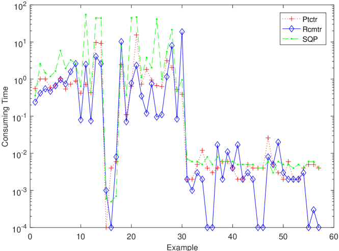
Figure 1: The computational time (s) of Ptctr,  Rcmtr and SQP for test problems.

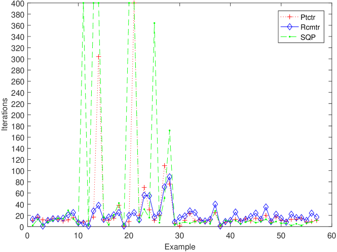
Figure 2: The number of iterations of Ptctr,  Rcmtr and SQP for test problems.

We test those $57$ problems with $n=2$ to $n\approx 1000$. The numerical results are arranged in Tables 1-2 for the convex problems, and Tables 3-4 for the non-convex problems. The computational time and the number of iterations of Rcmtr, Ptctr and SQP are illustrated in Figure 1 and Figure 2, respectively. From Table 1 and Table 2, we find that Rcmtr can solve those convex optimization problems with linear equality constraints well. However, there are 3 convex problems of 17 convex test problems can not be solved by Ptctr and SQP, respectively. ADMM can not work well for those 17 test convex problems.

From Table 3 and Table 4, we find that Rcmtr can solve those 40 non-convex linearly constrained optimization problems well except for a particularly difficult problem (Strectched V Function SB2013 ). For this problem, Ptctr and SQP can not solve it, too. Ptctr and SQP can not solve two non-convex problems and five non-convex problems of 40 non-convex problems, respectively. Furthermore, from Tables 2-4 and Figure 1, we find that the computational time of Rcmtr is significantly less than those of Ptctr and SQP for most of test problems, respectively. The computational time of Rcmtr is about 1/3 of that of SQP (fmincon.m).

From the numerical results, we find that Rcmtr works significantly better than the other three methods. One of the reasons is that Rcmtr uses the L-BFGS method (36) as the preconditioned technique to follow their trajectories in the well-posed phase. Consequently, Rcmtr only involves three pairs of the inner product of two vectors and one matrix-vector product ($p_{g_{k}}=Pg_{k}$) to obtain the trial step $s_{k}$ and involves about $(n-m)n$ flops at every iteration in the well-posed phase. However, Ptctr needs to solve a linear system of equations with an $n\times n$ symmetric positive definite coefficient matrix and involves about $\frac{1}{3}n^{3}$ flops (p. 169, GV2013 ) at every iteration. SQP needs to solve a linear system of equations with dimension $(m+n)$ when it solves a quadratic programming subproblem at every iteration (pp. 531-532, NW1999 ) and involves about $\frac{2}{3}(m+n)^{3}$ flops (p. 116, GV2013 ).

Table 1: Numerical results of Rcmtr and ADMM for convex problems.

Problems	Rcmtr		ADMM
	steps (time)	$f(x^{\star})$ (KKT)	steps (time)	$f(x^{\star})$ (KKT)
Exam. 1 Kim Problem 1 Kim2010 ; LLS2021 (n = 1000, m = n/2)	13 (0.24)	7.27e+03 (3.44e-07)	3 (0.04)	2.20e+04 (40.00) (failed)
Exam. 2 LLS Problem 1 LLS2021 (n = 1200, m = n/3)	17 (0.42)	1.44e+03 (9.37e-07)	21 (0.07)	2.73e+03 (4.00) (failed)
Exam. 3 Obsborne Problem 1 LLS2021 ; Osborne2016 (n = 1200, m = 2/3n)	1 (0.55)	7.15e+02 (1.27e-15)	60 (0.18)	8.48e+02 (2.80) (failed)
Exam. 4 Mak Problem LLS2021 ; MAK2019 (n = 1000, m = n/2)	11 (0.47)	97.96 (7.74e-07)	4 (0.05)	1.32e+02 (1.00) (failed)
Exam. 5 LLS Problem 2 LLS2021 (n = 1000, m = n/2)	14 (0.66)	82.43 (7.54e-08)	12 (0.04)	8.00e+03 (32.00) (failed)
Exam. 6 Osborne Problem 2 LLS2021 ; Osborne2016 (n = 1200, m = n/2)	14 (0.97)	5.14e+02 (8.75e-07)	60 (0.20)	7.86e+02 (2.80) (failed)
Exam. 7 Carlberg Problem Carlberg2009 ; LLS2021 (n = 1000, m = n/2)	15 (0.74)	1.19e+04 (1.66e-06)	3 (0.04)	1.40e+04 (32.00) (failed)
Exam. 8 Kim Problem 2 Kim2010 ; LLS2021 (n = 1000, m = n/2)	21 (1.59)	4.22e+04 (1.43e-06)	3 (0.33)	3.28e+05 (1.92e+03) (failed)
Exam. 9 Yamashita Problem LLS2021 ; Yamashita1980 (n = 1200, m = n/3)	25 (2.62)	0.50 (3.67e-07)	16 (0.06)	25.10 (0.50) (failed)
Exam. 10 Quartic With Noise Function AD2005 (n = 1000, m = n/2)	7 (0.08)	1.01e+02 (2.69e-07)	400 (0.40)	1.01e+02 (3.98) (failed)
Exam. 11 Rotated Hyper Ellopsoid Function SB2013 (n = 1000, m = n/2)	6 (2.50)	1.25e+05 (8.30e-06)	400 (1.04)	1.26e+05 (2.00e+05) (failed)
Exam. 12 Sphere Function SB2013 (n = 1000, m = n/2)	1 (0.08)	1.67e+02 (3.13e-15)	400 (0.27)	1.67e+02 (2.00) (failed)
Exam. 13 Sum Squares Function SB2013 (n = 1000, m = n/2)	28 (4.08)	4.08e+04 (1.58e-06)	400 (0.32)	4.16e+04 (9.98e+02) (failed)
Exam. 14 Trid Function SB2013 (n = 1000, m = n/2)	38 (2.61)	5.82e+02 (5.36e-07)	400 (0.36)	5.85e+02 (3.99) (failed)
Exam. 15 Booth Function SB2013 (n = 2, m = n/2)	13 (1.00e-03)	9.00 (1.98e-07)	18 (1.00e-03)	45.00 (30.00) (failed)
Exam. 16 Matyas Function SB2013 (n = 2, m = n/2)	17 (1.00e-04)	0.18 (4.44e-07)	18 (2.00e-03)	2.60 (5.20) (failed)
Exam. 17 Zakharov Function SB2013 (n = 10, m = n/2)	21 (8.00e-03)	7.31 (1.65e-07)	21 (1.00e-03)	4.33e+02 (1.87e+03) (failed)

Table 2: Numerical results of Ptctr, Rcmtr and SQP for convex problems.

Problems	Ptctr		Rcmtr		SQP
	steps (time)	$f(x^{\star})$ (KKT)	steps (time)	$f(x^{\star})$ (KKT)	steps (time)	$f(x^{\star})$ (KKT)
Exam. 1 Kim Problem 1 Kim2010 ; LLS2021 (n = 1000, m = n/2)	11 (0.56)	7.27e+03 (5.79e-08)	13 (0.24)	7.27e+03 (3.44e-07)	2 (0.36)	7.27e+03 (8.30e-13)
Exam. 2 LLS Problem 1 LLS2021 (n = 1200, m = n/3)	17 (1.01)	1.44e+03 (7.36e-07)	17 (0.42)	1.44e+03 (9.37e-07)	13 (2.59)	1.44e+03 (3.42e-07)
Exam. 3 Obsborne Problem 1 LLS2021 ; Osborne2016 (n = 1200, m = 2/3n)	12 (1.01)	7.15e+02 (2.30e-07)	1 (0.55)	7.15e+02 (1.27e-15)	3 (1.48)	7.14e+02 (2.22e-15)
Exam. 4 Mak Problem LLS2021 ; MAK2019 (n = 1000, m = n/2)	11 (0.59)	97.96 (3.50e-07)	11 (0.47)	97.96 (7.74e-07)	8 (1.18)	97.96 (1.34e-10)
Exam. 5 LLS Problem 2 LLS2021 (n = 1000, m = n/2)	14 (0.69)	82.43 (8.79e-08)	14 (0.66)	82.43 (7.54e-08)	11 (1.65)	82.43 (1.78e-09)
Exam. 6 Osborne Problem 2 LLS2021 ; Osborne2016 (n = 1200, m = n/2)	13 (1.04)	5.14e+02 (1.79e-07)	14 (0.97)	5.14e+02 (8.75e-07)	15 (5.86)	5.14e+02 (1.75e-06)
Exam. 7 Carlberg Problem Carlberg2009 ; LLS2021 (n = 1000, m = n/2)	10 (0.54)	1.19e+04 (1.23e-07)	15 (0.74)	1.19e+04 (1.66e-06)	14 (1.96)	1.19e+04 (1.13e-05)
Exam. 8 Kim Problem 2 Kim2010 ; LLS2021 (n = 1000, m = n/2)	12 (0.73)	4.22e+04 (6.14e-06)	21 (1.59)	4.22e+04 (1.43e-06)	29 (3.27)	4.22e+04 (3.05e-06)
Exam. 9 Yamashita Problem LLS2021 ; Yamashita1980 (n = 1200, m = n/3)	16 (0.89)	0.50 (4.39e-07)	25 (2.62)	0.50 (3.67e-07)	14 (2.64)	0.50 (1.01e-07)
Exam. 10 Quartic With Noise Function AD2005 (n = 1000, m = n/2)	9 (0.42)	1.01e+02 (3.14e-07)	7 (0.08)	1.01e+02 (2.69e-07)	4 (0.64)	1.01e+02 (1.25e-09)
Exam. 11 Rotated Hyper Ellopsoid Function SB2013 (n = 1000, m = n/2)	8 (0.72)	1.25e+05 (2.08e-04) (failed)	6 (2.50)	1.25e+05 (8.30e-06)	400 (55.18)	1.46e+05 (3.22e+02) (failed)
Exam. 12 Sphere Function SB2013 (n = 1000, m = n/2)	10 (0.43)	1.67e+02 (1.11e-07)	1 (7.50e-02)	1.67e+02 (3.13e-15)	3 (0.44)	1.67e+02 (7.67e-10)
Exam. 13 Sum Squares Function SB2013 (n = 1000, m = n/2)	17 (9.77)	4.08e+04 (1.85e-04) (failed)	28 (4.08)	4.08e+04 (1.58e-06)	400 (44.36)	4.10e+04 (1.01e+02) (failed)
Exam. 14 Trid Function SB2013 (n = 1000, m = n/2)	304 (9.18)	5.82e+02 (8.34e-04) (failed)	38 (2.61)	5.82e+02 (5.36e-07)	400 (44.05)	5.82e+02 (1.56e-04) (failed)
Exam. 15 Booth Function SB2013 (n = 2, m = n/2)	12 (1.00e-04)	9.00 (1.74e-07)	13 (1.00e-03)	9.00 (1.98e-07)	17 (6.00e-03)	9.00 (3.55e-15)
Exam. 16 Matyas FunctionSB2013 (n = 2, m = n/2)	11 (4.00e-03)	0.18 (1.87e-08)	17 (1.00e-04)	0.18 (4.44e-07)	3 (5.00e-03)	0.18 (1.67e-16)
Exam. 17 Zakharov FunctionSB2013 (n = 10, m = n/2)	15 (6.00e-03)	7.31 (2.93e-08)	21 (8.00e-03)	7.31 (1.65e-07)	21 (7.00e-03)	7.31 (8.50e-06)

Table 3: Numerical results of Ptctr, Rcmtr, SQP for large-scale nonconvex problems.

Problems	Ptctr		Rcmtr		SQP
	steps (time)	$f(x^{\star})$ (KKT)	steps (time)	$f(x^{\star})$ (KKT)	steps (time)	$f(x^{\star})$ (KKT)
Exam. 18 LLS Problem 3 LLS2021 (n = 1000, m = n/2)	38 (2.45)	1.96e+02 (1.17e-05)	25 (10.27)	-3.03e+03 (4.86e-07)	42 (7.70)	1.88e+02 (7.97e-06)
Exam. 19 Ackly Function SB2013 (n = 1000, m = n/2)	1 (0.11)	2.64 (1.87e-07)	1 (7.10e-02)	2.64 (7.50e-07)	2 (0.37)	2.42 (1.94e-07)
Exam. 20 Rosenbrock Function SB2013 (n = 1000, m = n/2)	9 (0.64)	9.26e+03 (9.03e-06)	20 (0.78)	9.26e+03 (2.15e-06)	400 (44.68)	9.26e+03 (5.00e-03) (failed)
Exam. 21 Dixon-Price Function SB2013 (n = 1000, m = n/2)	400 (15.54)	8.97e+04 (2.42e-02) (failed)	25 (2.35)	9.00e+04 (1.74e-09)	400 (46.97)	8.24e+06 (1.28e+05) (failed)
Exam. 22 Griewank Function SB2013 (n = 1000, m = n/2)	20 (0.73)	0.86 (4.81e-07)	12 (0.35)	0.86 (4.40e-08)	9 (1.12)	0.86 (1.07e-10)
Exam. 23 Levy Function SB2013 (n = 1000, m = n/2)	70 (1.83)	71.06 (2.36e-08)	56 (0.12)	71.06 (8.25e-07)	31 (3.82)	71.06 (1.11e-07)
Exam. 24 Molecular Energy Function ML2004 (n = 1000, m = n/2)	30 (0.94)	4.69e+02 (4.38e-07)	55 (0.75)	4.69e+02 (8.66e-07)	16 (2.04)	4.69e+02 (1.71e-06)
Exam. 25 Powell Function SB2013 (n = 1000, m = n/2)	11 (0.67)	4.26e+03 (1.77e-06)	17 (9.50e-02)	4.26e+03 (4.52e-07)	364 (41.34)	4.26e+03 (1.38e-04) (failed)
Exam. 26 Rastrigin Function SB2013 (n = 1000, m = n/2)	20 (0.63)	2.93e+03 (6.42e-07)	24 (0.11)	2.93e+03 (1.56e-06)	7 (1.00)	4.44e+03 (1.13e-06)
Exam. 27 Schwefel Function SB2013 (n = 1000, m = n/2)	109 (3.17)	4.19e+05 (3.74e-07)	71 (1.16)	4.19e+05 (4.16e-06)	51 (5.49)	4.02e+05 (2.31e-06)
Exam. 28 Styblinski Tang Function SB2013 (n = 1000, m = n/2)	76 (2.05)	-9.61e+03 (1.12e-05)	89 (8.02)	-9.61e+03 (4.57e-06)	172 (21.46)	-2.56e+04 (7.03e-04) (failed)
Exam. 29 Shubert Function SB2013 (n = 1000, m = n/2)	6 (0.53)	2.65e+03 (1.43e-06)	8 (8.40e-02)	2.65e+03 (8.92e-07)	3 (0.47)	2.65e+03 (1.42e-05)
Exam. 30 Strectched V Function SB2013 (n = 1000, m = n/2)	1 (0.39)	3.10e-03 (1.08e+05) (failed)	16 (18.86)	2.30e+02 (2.41e-03) (failed)	6 (0.95)	1.28 (34.15) (failed)

Table 4: Numerical results of Ptctr, Rcmtr, SQP for small-scale nonconvex problems.

Problems	Ptctr		Rcmtr		SQP
	steps (time)	$f(x^{\star})$ (KKT)	steps (time)	$f(x^{\star})$ (KKT)	steps (time)	$f(x^{\star})$ (KKT)
Exam. 31 Beale Function SB2013 (n = 2, m = n/2)	11 (2.00e-03)	3.35 (2.23e-08)	19 (2.00e-03)	3.35 (8.92e-07)	8 (7.00e-03)	3.35 (1.50e-06)
Exam. 32 Branin Function SB2013 (n = 2, m = n/2)	23 (2.00e-03)	15.90 (1.51e-08)	28 (1.00e-03)	15.90 (3.53e-07)	6 (6.00e-03)	34.37 (4.55e-06)
Exam. 33 Eason Function SB2013 (n = 2, m = n/2)	10 (5.00e-03)	-4.19e-06 (4.08e-06)	25 (3.00e-03)	-4.19e-06 (1.06e-07)	9 (6.00e-03)	-4.55e-06 (5.80e-07)
Exam. 34 Hosaki Function AD2005 (n = 2, m = n/2)	12 (1.20e-02)	-0.56 (4.21e-07)	11 (2.00e-03)	-0.56 (3.24e-08)	6 (5.00e-03)	-0.56 (9.77e-07)
Exam. 35 Levy Function N. 13 SB2013 (n = 2, m = n/2)	8 (4.00e-03)	0.63 (9.51e-07)	10 (1.00e-04)	0.63 (1.61e-07)	9 (8.00e-03)	0.98 (1.42e-05)
Exam. 36 McCormick Function SB2013 (n = 12, m = n/2)	12 (3.00e-03)	1.31 (1.05e-07)	13 (1.00e-04)	1.31 (8.42e-07)	5 (5.00e-03)	1.31 (2.64e-09)
Exam. 37 Perm Function $d,\ \beta$ SB2013 (n = 4, m = n/2)	25 (4.00e-03)	1.19e+03 (2.59e-06)	40 (1.70e-02)	1.19e+03 (3.85e-06)	28 (8.00e-03)	1.19e+03 (7.41e-05)
Exam. 38 Power Sum Function SB2013 (n = 4, m = n/2)	1 (6.00e-03)	1.52e+04 (2.59e-06)	1 (2.00e-03)	1.52e+04 (1.85e-13)	2 (6.00e-03)	1.52e+04 (1.14e-12)
Exam. 39 Price Function AD2005 (n = 2, m = n/2)	8 (6.00e-03)	7.06 (1.50e-07)	9 (1.10e-02)	7.06 (1.85e-07)	11 (6.00e-03)	7.06 (7.77e-06)
Exam. 40 Bohachevsky Function SB2013 (n = 2, m = n/2)	9 (4.00e-03)	2.36 (1.75e-07)	11 (4.00e-03)	2.36 (7.12e-07)	9 (6.00e-03)	1.15 (1.00e-08)
Exam. 41 Colville Function SB2013 (n = 4, m = n/2)	13 (2.00e-03)	21.14 (1.35e-07)	26 (1.70e-02)	21.14 (5.81e-07)	11 (5.00e-03)	5.19 (3.37e-05)
Exam. 42 Drop Wave Function SB2013 (n = 2, m = n/2)	10 (2.00e-03)	-0.79 (2.12e-07)	9 (2.00e-03)	-0.7858 (9.15e-07)	5 (5.00e-03)	-0.79 (3.73e-09)
Exam. 43 Schaffer Function SB2013 (n = 2, m = n/2)	14 (5.00e-03)	0.61 (7.18e-08)	13 (3.00e-03)	0.61 (1.04e-07)	8 (5.00e-03)	0.61 (1.62e-07)
Exam. 44 Six-Hump Camel Function SB2013 (n = 2, m = n/2)	10 (4.00e-03)	0.74 (1.73e-07)	18 (2.00e-03)	0.74 (4.09e-07)	11 (5.00e-03)	0.74 (2.00e-08)
Exam. 45 Three-Hump Camel Function SB2013 (n = 2, m = n/2)	15 (4.00e-03)	0.55 (3.91e-07)	24 (1.00e-04)	0.55 (4.82e-07)	7 (4.00e-03)	0.55 (1.46e-07)
Exam. 46 Trecanni Function AD2005 (n = 2, m = n/2)	11 (4.00e-03)	2.36 (2.78e-08)	13 (1.00e-04)	2.36 (4.91e-07)	9 (4.00e-03)	2.36 (4.19e-08)
Exam. 47 Box Bettes Exponential Quadratic Function AD2005 (n = 3, m = 2)	20 (2.60e-02)	1.42e-11 (9.96e-07)	35 (8.00e-03)	3.01e-13 (7.07e-07)	13 (6.00e-03)	3.26e-16 (2.57e-08)
Exam. 48 Chichinad Function AD2005 (n = 2, m = n/2)	8 (5.00e-03)	8.01 (9.15e-09)	9 (5.00e-03)	8.01 (4.47e-08)	6 (3.00e-03)	-20.06 (8.52e-07)
Exam. 49 Eggholder Function SB2013 (n = 2, m = n/2)	17 (3.00e-03)	-69.16 (4.17e-07)	22 (2.00e-02)	-69.60 (9.45e-07)	9 (6.00e-03)	-69.16 (5.77e-08)
Exam. 50 Exp2 Function AD2005 (n = 2, m = n/2)	11 (2.00e-03)	9.19 (1.53e-08)	15 (3.00e-03)	8.45 (6.63e-07)	6 (5.00e-03)	9.19 (6.60e-07)
Exam. 51 Hansen Function AD2005 (n = 2, m = n/2)	9 (6.00e-03)	-12.10 (3.98e-08)	8 (2.00e-03)	-12.10 (1.69e-07)	6 (5.00e-03)	-32.36 (5.21e-05)
Exam. 52 Hartmann 3-D Function SB2013 (n = 3, m = 2)	13 (2.00e-03)	-3.84 (1.36e-07)	22 (2.00e-03)	-3.84 (8.13e-07)	2 (4.00e-03)	-1.31e-30 (2.22e-16)
Exam. 53 Holder Table Function SB2013 (n = 2, m = n/2)	13 (2.00e-03)	-1.68 (1.65e-07)	16 (2.00e-03)	-1.68 (5.82e-07)	5 (5.00e-03)	-3.51e-02 (9.62e-07)
Exam. 54 Michalewicz Function SB2013 (n = 2, m = n/2)	15 (4.00e-03)	-1.00 (7.24e-08)	16 (3.00e-03)	-1.00 (6.12e-07)	2 (4.00e-03)	-7.18e-12 (1.20e-10)
Exam. 55 Schaffer Function N. 4 SB2013 (n = 4, m = n/2)	8 (5.00e-03)	0.30 (9.11e-07)	11 (1.00e-04)	0.30 (8.35e-07)	6 (6.00e-03)	0.29 (7.68e-07)
Exam. 56 Trefethen 4 Function AD2005 (n = 2, m = n/2)	9 (5.00e-03)	1.20 (7.61e-08)	24 (3.00e-04)	-1.36 (1.51e-07)	8 (6.00e-03)	-2.02 (7.45e-05)
Exam. 57 Zettl Function AD2005 (n = 2, m = n/2)	11 (4.00e-03)	0.14 (3.26e-08)	17 (1.00e-04)	0.14 (8.27e-07)	11 (4.00e-03)	0.14 (1.84e-09)

5 Conclusions

In this paper, we give the regularization continuation method with the trust-region updating strategy (Rcmtr) for linearly constrained optimization problems. Moreover, we reveals and utilizes the linear conservation law of the regularization method and the quasi-Newton method such that it does not need to compute the correction step other than the previous continuation method. The new continuation method uses the inverse of the regularization two-sided projection of the Lagrangian Hessian as the pre-conditioner to improve its robustness, which is other than the previous quasi-Newton methods. Numerical results show that Rcmtr is more robust and faster than the traditional optimization method such as SQP (the built-in subroutine fmincon.m of the MATLAB2020a environment MATLAB ), the recent continuation method such as Ptctr LLS2021 and the alternating direction method of multipliers (ADMM BPCE2011 ). Therefore, Rcmtr is worth exploring further, and we will extend it to the nonlinearly constrained optimization problem in the future.

References

(1)
E. P. Adorio and U. P. Diliman, MVF - Multivariate test functions
library in C for unconstrained global optimization,
http://www.geocities.ws/eadorio/mvf.pdf, 2005.
(2)
E. L. Allgower and K. Georg, Introduction to Numerical
Continuation Methods, SIAM, Philadelphia, PA, 2003.
(3)
U. M. Ascher and L. R. Petzold, Computer Methods for Ordinary
Differential Equations and Differential-Algebraic Equations, SIAM,
Philadelphia, PA, 1998.
(4)
J. M. Bioucas-Dias and M. A. T. Figueiredo, Alternating direction
algorithms for constrained sparse regression: Application to hyperspectral unmixing,
2010 2nd Workshop on Hyperspectral Image and Signal Processing: Evolution in Remote
Sensing, 2010, 1-4, http://doi.org/10.1109/WHISPERS.2010.5594963.
(5)
C. G. Broyden, The convergence of a class of double-rank minimization algorithms,
J Inst Math Appl 6 (1970), 76-90.
(6)
A. A. Brown and M. C. Bartholomew-Biggs, ODE versus SQP methods for
constrained optimization, J Optim Theory Appl 62 (1989), 371-386.
(7)
K. E. Brenan, S. L. Campbell and L. R. Petzold, Numerical solution of
initial-value problems in differential-algebraic equations, SIAM, Philadelphia,
PA, 1996.
(8)
J. C. Butcher and Z. Jackiewicz, Construction of high order diagonally implicit
multistage integration methods for ordinary differential equations, Appl Numer
Math 27 (1998), 1-12.
(9)
S. Boyd, N. Parikh, E. Chu, B. Peleato and J. Eckstein, Distributed optimization
and statistical learning via the alternating direction method of multipliers,
Found Trends Mach Learn 3 (2011), 1-122, software available
at https://web.stanford.edu/~boyd/papers/admm/.
(10)
R. Byrd, J. Nocedal and Y. X. Yuan, Global convergence of a class of
quasi-Newton methods on convex problems, SIAM J Numer Anal 24 (1987),
1171-1189.
(12)
F. Caballero, L. Merino, J. Ferruz and A. Ollero, Vision-based odometry
and SLAM for medium and high altitude flying UAVs, J Intell Robot Syst
54 (2009), 137-161.
(13)
T. S. Coffey, C. T. Kelley and D. E. Keyes, Pseudotransient
continuation and differential-algebraic equations, SIAM J Sci Comput
25 (2003), 553-569.
(14)
A. R. Conn, N. Gould and Ph. L. Toint, Trust-Region Methods,
SIAM, Philadelphia, USA, 2000.
(15)
M. T. Chu and M. M. Lin, Dynamical system characterization of the central path
and its variants- a vevisit, SIAM J Appl Dyn Syst 10 (2011), 887-905.
(16)
J. M. Fadili, J. L. Starck, Monotone operator splitting for optimization
problems in sparse recovery, IEEE ICIP, Nov 2009, Cairo, Egypt.,
1461-1464, http://doi.org/10.1109/ICIP.2009.5414555.
(17)
A. V. Fiacco and G. P. McCormick, Nonlinear programming: Sequential
Unconstrained Minimization Techniques, SIAM, 1990.
(18)
M. A. T. Figueiredo and J. M. Bioucas-Dias, Restoration of
Poissonian images using alternating direction optimization,
IEEE Trans Image Process 19 (2010), 3133-3145.
(19)
R. Fletcher, A new approach to variable metric algorithms, Comput J
13 (1970), 317-322.
(20)
R. Fletcher and M. J. D. Powell, A rapidly convergent descent method for
minimization, Comput J 6 (1963), 163-168.
(21)
P. A. Forero, A. Cano and G. B. Giannakis, Consensus-based distributed
support vector machines, J Mach Learn Res 11 (2010), 1663-1707.
(22)
B. S. Goh, Approximate greatest descent methods for optimization with
equality constraints, J Optim Theory Appl 148 (2011), 505-527.
(23)
D. Goldfarb, A family of variable metric updates derived by variational means,
Math Comput 24 (1970), 23-26.
(24)
G. H. Golub and C. F. Van Loan, Matrix Computations, 4th ed., The Johns
Hopkins University Press, Baltimore, Mayryland, 2013.
(25)
E. Hairer, C. Lubich and G. Wanner, Geometric Numerical Integration:
Structure-Preserving Algorithms for Ordinary Differential Equations, 2nd ed.,
Springer, Berlin, 2006.
(26)
P. C. Hansen, Regularization Tools: A MATLAB package for analysis and solution
of discrete ill-posed problems, Numer Algorithms 6 (1994), 1-35.
(27)
U. Helmke and J. B. Moore, Optimization and Dynamical Systems, 2nd ed.,
Springer-Verlag, London, 1996.
(28)
D. J. Higham, Trust region algorithms and timestep selection, SIAM J Numer
Anal 37 (1999), 194-210.
(29)
Z. Jackiewicz and S. Tracogna, A general class of two-step Runge-Kutta methods for
ordinary differential equations, SIAM J Numer Anal 32 (1995), 1390-1427.
(30)
C. T. Kelley, L.-Z. Liao, L. Qi, M. T. Chu, J. P. Reese and C.
Winton, Projected Pseudotransient Continuation, SIAM J Numer Anal
46 (2008), 3071-3083.
(32)
J. H. Lee, Y. M Jung, Y. X. Yuan and S. Yun, A subsapce SQP method for
equality constrained optimization, Comput Optim Appl 74 (2019),
177-194.
(33)
K. Levenberg, A method for the solution of certain problems in least squares,
Q Appl Math 2 (1944), 164-168.
(34)
L.-Z. Liao, H. D. Qi, and L. Q. Qi, Neurodynamical optimization,
J Glob Optim 28 (2004), 175-195.
(35)
X.-L. Luo, Singly diagonally implicit Runge-Kutta methods
combining line search techniques for unconstrained optimization,
J Comput Math 23 (2005), 153-164.
(36)
X.-L. Luo, L.-Z. Liao and H.-W. Tam, Convergence analysis of
the Levenberg-Marquardt method, Optim Methds Softw 22 (2007), 659-678.
(37)
S.-T. Liu and X.-L. Luo, A method based on Rayleigh quotient gradient
flow for extreme and interior eigenvalue problems,Linear Algebra Appl
432 (2010), 1851-1863.
(38)
X.-L. Luo, A dynamical method of DAEs for the smallest eigenvalue
problem, J Comput Sci 3 (2012), 113-119.
(39)
X.-L. Luo, J.-R. Lin and W.-L. Wu, A prediction-correction dynamic
method for large-scale generalized eigenvalue problems, Abstr Appl Anal (2013),
Article ID 845459, 1-8, http://dx.doi.org/10.1155/2013/845459.
(40)
X.-L. Luo, J.-H. Lv and G. Sun, Continuation methods with the trusty time-stepping
scheme for linearly constrained optimization with noisy data, Optim Eng (2021),
published online at http://doi.org/10.1007/s11081-020-09590-z, 1-35.
(41)
X.-L. Luo, H. Xiao and J.-H. Lv, Continuation Newton methods with the
residual trust-region time-stepping scheme for nonlinear equations, Numer
Algorithms (2021), published online at http://doi.org/10.1007/s11075-021-01112-x,
1-25.
(42)
X.-L. Luo and Y.-Y. Yao, Primal-dual path-following methods and the trust-region
updating strategy for linear programming with noisy data, J Comput Math (2021),
published online at http://doi.org/10.4208/jcm.2101-m2020-0173, 1-21.
(43)
X.-L. Luo, H. Xiao, J.-H. Lv and S. Zhang, Explicit pseudo-transient
continuation and the trust-region updating strategy for unconstrained optimization,
Appl Numer Math 165 (2021), 290-302.
(44)
X.-L. Luo and H. Xiao,Generalized continuation Newton methods and the
trust-region updating strategy for the underdetermined system, J Sci Comput,
88 (2021), published online at
http://doi.org/10.1007/s10915-021-01566-0, pp. 1-22, July 13, 2021.
(46)
Z. S. Lu, K. K. Pong and Y. Zhang, An alternating direction method for
finding Dantzig selectors, Comput Stat Data Anal 56 (2012),
4037-4046, https://doi.org/10.1016/j.csda.2012.04.019.
(47)
M. F. Mascarenhas, The BFGS method with exact line searches fails for
non-convex objective functions, Math Program 99 (2004), 49-61.
(50)
D. Marquardt, An algorithm for least-squares estimation of nonlinear parameters,
SIAM J Appl Math 11 (1963), 431-441.
(51)
N. Maculan and C. Lavor, A function to test methods applied
to global minimization of potential energy of molecules, Numer Algorithms,
35 (2004), 287-300.
(52)
M. Ng, P. Weiss and X.-M. Yuan, Solving constrained total-variation image
restoration and reconstruction problems via alternating direction methods,
SIAM J Sci Comput 32 (2010), 2710-2736, http://doi.org/10.1137/090774823.
(53)
J. Nocedal and S. J. Wright, Numerical Optimization,
Springer-Verlag, Berlin, 1999.
(55)
P.-Q. Pan, New ODE methods for equality constrained optimization (2):
algorithms, J Comput Math 10 (1992), 129-146.
(56)
M. J. D. Powell, Convergence properties of a class of minimization
algorithms, in: O.L. Mangasarian, R. R. Meyer and S. M. Robinson,
eds., Nonlinear Programming 2, Academic Press, New York, pp. 1-27, 1975.
(57)
J. Schropp, A dynamical systems approach to constrained minimization,
Numer Funct Anal Optim 21 (2000), 537-551.
(58)
J. Schropp, One and multistep discretizations of index 2
differential algebraic systems and their use in optimization,
J Comput Appl Math 150 (2003), 375-396.
(59)
L. F. Shampine, Linear conservation laws for ODEs, Comput Math Appl
35 (1998), 45-53.
(60)
L. F. Shampine, Conservation laws and the numerical solution of ODEs II,
Comput Math Appl 38 (1999), 61-72.
(61)
L. F. Shampine, I. Gladwell and S. Thompson, Solving ODEs with MATLAB,
Cambridge University Press, Cambridge, 2003.
(62)
D. F. Shanno, Conditioning of quasi-Newton methods for function minimization,
Math Comput 24 (1970), 647-656.
(63)
G. Steidl and T. Teuber, Removing multiplicative noise by Douglas-Rachford
splitting methods, J Math Imaging Vis 36 (2010), 168-184.
(64)
S. Surjanovic and D. Bingham, Virtual library of simulation
experiments: Test functions and datasets, retrieved from
http://www.sfu.ca/~ssurjano, January 2020.
(65)
W. Y. Sun and Y. X. Yuan, Optimization Theory and Methods: Nonlinear
Programming, Springer, New York, 2006.
(66)
K. Tanabe, A geometric method in nonlinear programming, J Optim Theory
Appl 30 (1980), 181-210.
(67)
A. N. Tikhonov and V. Y. Arsenin, Solutions of Ill-posed Problems,
John Wiley & Sons, New York, Toronto, London, 1977.
(68)
N. Ullah, J. Sabi’u and A. Shah, A derivative-free scaled memoryless BFGS
method for solving a system of monotone nonlinear equations, Numer
Linear Algebra Appl. 2021;e2374. https://doi.org/10.1002/nla.2374.
(69)
R. Vanderbei, K. Lin, H. Liu and L. Wang, Revisiting compressed sensing:
exploiting the efficiency of simplex and sparsification methods,
Math Prog Comp 8 (2016), 253–269,
http://doi.org/10.1007/s12532-016-0105-y.
(70)
R. B. Wilson, A Simplicial Method for Convex Programming, Ph.D. thesis,
Harvard University, 1963.
(71)
H. Yamashita, A differential equation approach to nonlinear programming,
Math Program 18 (1980), 155-168.
(72)
Y. Yuan, Recent advances in trust region algorithms, Math Program
151 (2015), 249-281.