Compressible test-field method and its application to shear dynamos

Abstract

In this study we present a compressible test-field method (CTFM) for computing $\alpha$ effect and turbulent magnetic diffusivity tensors, as well as those relevant for mean ponderomotive force and mass source, applied to the full MHD equations. We describe the theoretical background of the method, and compare it to the quasi-kinematic test-field method, and to the previously studied variant working in simplified MHD (SMHD). We present several test cases using velocity and magnetic fields of the Roberts geometry, and also compare with the imposed-field method. We show that, for moderate imposed field strengths, the nonlinear CTFM (nCTFM) gives results in agreement with the imposed-field method. Comparison of different flavors of the nCTFM in the shear dynamo case also agree up to equipartition field strengths. Some deviations between the CTFM and SMHD variants exist. As a relevant physical application, we study non-helically forced shear flows, which exhibit large-scale dynamo action, and present a re-analysis of low Reynolds number, moderate shear systems, where we previously neglected the pressure gradient in the momentum equation, and found no coherent shear-current effect. Another key difference is that in the earlier study we used magnetic forcing to mimic small-scale dynamo action, while here it is self-consistently driven by purely kinetic forcing. The kinematic CTFM with general validity forms the core of our analysis. We still find no coherent shear-current effect, but do recover strong large-scale dynamo action that, according to our analysis, is driven through the incoherent effects.

1 Introduction

Over the past few decades, both local and global numerical simulations of accretion discs have demonstrated that magnetic fields can be generated by a dynamo and drive turbulent accretion through what is believed to be the magneto-rotational instability (Brandenburg et al., 1995; Hawley et al., 1996; Hawley, 2000). Real discs are always stratified about the midplane, which can lead to kinetic helicity and thereby to an $\alpha$ affect. Whether or not this really explains what is seen in numerical simulations is unclear, because there are other, potentially more powerful alternatives. One of them is the shear-current (SC) effect. It is a mean-field dynamo effect that can, in principle, generate large-scale magnetic fields based on the off-diagonal components of the turbulent magnetic diffusivity tensor (Rogachevskii & Kleeorin, 2003, 2004). Whether or not this effect can also be responsible for the large-scale dynamo (LSD) seen in some non-helically forced shear flows continues to raise debate (see, e.g., the recent papers Squire & Bhattacharjee, 2016; Käpylä et al., 2020; Zhou & Blackman, 2021, with contradictory results for and against). Such a dynamo has been proposed to avoid the need for the more classical helicity-based $\alpha$ effect in situations where stratification and rotation are ineffective or absent, and hence neither kinetic helicity nor $\alpha$ effect can arise. One major cause of the aforementioned contradictions arises from the fact that, methodologically, a reliable quantitative measurement device capable of returning the turbulent transport coefficients for an MHD background turbulence due to a small-scale dynamo (SSD) in full MHD has not been available.

The imposed-field method was the first machinery developed in the 1990’s (Brandenburg et al., 1990) for the retrieval of $\alpha$ effect and turbulent pumping by imposing uniform magnetic fields in different directions, measuring the mean (a.k.a. turbulent) electromotive force (EMF), and solving for the unknown coefficients. Gradients of the mean field contribute to the mean EMF via the turbulent diffusivity tensor, hence it is important to guarantee that they remain weak in the evolving magnetic field. Therefore, the field has to be reset after suitable time intervals, and not taking this into account properly has led to some misinterpretations of the results (see the discussion in Ossendrijver et al., 2001; Käpylä et al., 2010, and the references therein). When properly used, this method continues to be a valuable tool, and is used also in this work to validate the test-field results in the simplest cases.

The next methodology was introduced by Brandenburg & Sokoloff (2002) as a method of moments: to tackle the large amount of unknown transport coefficients entering the mean EMF while there are only three equations relating it to the mean field, additional equations were constructed by forming a sufficient number of moments. Measuring them from the numerical models enables then to solve for the coefficients. This method can retrieve both the $\alpha$ and the turbulent resistivity tensors, but relies on the mean field, generated in the system, to be unsteady, typically oscillatory. This method has various incarnations in many astrophysical contexts (e.g. Squire & Bhattacharjee, 2015; Shi et al., 2016; Simard et al., 2016; Käpylä et al., 2018). Occasionally, however, it is employed in an improper way by pre-assuming some of the coefficients to be negligible; putting them deliberately to zero then renders the fitting meaningless in the worst case (e.g. Simard et al., 2013; Squire & Bhattacharjee, 2015; Shi et al., 2016).

The third alternative is the test-field method (TFM), introduced by Schrinner et al. (2005, 2007), where linearly independent test fields are subjected to the velocity taken from a simulation, including both its fluctuating and mean constituents. The test fields are passive, i.e., do not affect the course of the simulation itself (except possibly through the time step control). The equations for the corresponding fluctuating magnetic fields are solved, which then allows for retrieving the full set of tensor coefficients (Brandenburg et al., 2008b). If the simulation is purely hydrodynamic, this approach is kinematic, but if it is an MHD run, where the generated magnetic field does backreact on the flow, the method is called quasi-kinematic (QKTFM). For both variants, however, the same procedures apply. This method has proven immensely successful, and has been utilized within a broad spectrum of astrophysical stellar, planetary, and disk dynamo applications, including the shear dynamo problem (Brandenburg et al., 2008a). The QKTFM has been applied in Cartesian domains with and without shearing-periodic boundary conditions and horizontal ($xy$) averaging, as well as in spherical domains, with longitudinal averaging. The latter type of models (see e.g., Warnecke et al., 2018) has included rotation and stratification, and is hence not an optimal situation for clarifying whether or not the SC effect can be important. Also, it is not trivial to separate this effect from others contributing to the turbulent magnetic diffusivity tensor such as the Rädler effect with its antisymmetric contribution. When an SSD is excited in such setups, it is supposed to boost the SC effect (the scenario proposed by Squire & Bhattacharjee, 2016). The (Q)KTFM however, does not apply: SSD action generates a magnetic background turbulence, the magnetic part of which is not accounted for.

A core machinery towards a TFM, which can take into account the magnetic background turbulence, was presented by (Rheinhardt & Brandenburg, 2010), albeit relying on simplified MHD (SMHD), where pressure gradient and self-advection of the flow were dropped from the momentum equation. Another step further was taken in Käpylä et al. (2020), admitting self-advection, while yet ignoring the pressure gradient and hence variations of density. This study has been deemed inconclusive (see, e.g. Zhou & Blackman, 2021), as second-order correlation approximation (SOCA) calculations of Squire & Bhattacharjee (2016) were interpreted to indicate a decisive role of the pressure gradient in creating the magnetic SC effect. In contrast, we argued that the magnetic SC effect continues to exist in SMHD in the ideal limit, albeit with a sign not supportive for a mean-field dynamo. This paper aims at introducing a method meeting all requirements, namely the fully compressible test-field method (CTFM). We present test cases to prove its functionality, and then make a first attempt to apply it to the shear dynamo problem in the regime of moderate Reynolds number, magnetic Prandtl number, and shear, where we measure the turbulent transport coefficients and interpret them in the framework of mean-field dynamo theory.

We should clarify from the outset that our primary goal in the calculation of mean-field transport coefficients is at present not to utilize them in more economic mean-field models of astrophysical dynamos, but rather to provide some understanding of the turbulent processes found in the progressively more realistic simulations of such dynamos. In principle, our computations can also identify specific targets of what to look for in future studies. We further note that for the first steps to understand the SC effect with the CTFM, we use the simplest possible setup, excluding physically important effects such as rotation and stratification, thus studying this effect in isolation. This approach is chosen to gain physical insights about this effect, albeit not allowing us to assess its relevance in astrophysical objects.

2 Model and Methods

The full MHD (FMHD) system of equations, here with an isothermal equation of state, is more complex than that of SMHD used in earlier TFMs because of the occurrence of the pressure gradient. As a result, we need an additional evolution equation for the density, being the counterpart to the Poisson equation for the pressure in incompressible MHD. Also the viscous force is now more complex. Hence, we have

$${\cal D}{}^{A}\bm{A} = \bm{U}\times\bm{B}+\bm{F}_{\rm M}+\eta{\bm{\nabla}}^{2}\bm{A},$$ (1)

$$\!\!\!\!\!\rho({\cal D}{}^{U}\!+\bm{U}\!\cdot\!{\bm{\nabla}})\bm{U}+{\bm{\nabla}}P = \bm{J}\times\bm{B}+\rho\bm{F}_{\rm K}+{\bm{\nabla}}\!\cdot\!(2\nu\rho\boldsymbol{\mathsf{S}}),$$ (2)

$$({\cal D}{}+\bm{U}\cdot{\bm{\nabla}})\ln\rho = -{\bm{\nabla}}\cdot\bm{U},$$ (3)

where $\bm{J}={\bm{\nabla}}\times\bm{B}$ is the current density with the vacuum permeability set to unity. Furthermore,

$${\cal D}{}^{A}\bm{A} = {\cal D}{}\bm{A}+SA_{y}\hat{\mbox{\boldmath$x$}}{},$$ (4)

$${\cal D}{}^{U}\bm{U} = {\cal D}{}\bm{U}+SU_{x}\hat{\mbox{\boldmath$y$}}{}+2\bm{\Omega}\times\bm{U},$$ (5)

$${\cal D}{} = \partial_{t}+Sx\partial_{y}$$ (6)

are linear operators. Here, $\bm{\Omega}=\Omega\hat{\mbox{\boldmath$z$}}{}$ is the global angular velocity vector, ${\sf S}_{ij}=(U_{i,j}+U_{j,i})/2-\delta_{ij}{\bm{\nabla}}\cdot\bm{U}/3$ are the components of the traceless rate-of-strain tensor $\boldsymbol{\mathsf{S}}$, where commas denote partial differentiation, and $P$ is the pressure related to the density via $P=c_{\rm s}^{2}\rho$ with the isothermal sound speed $c_{\rm s}$. Terms containing $S$ are due to a linear background shear flow of the form $\bm{U}^{(S)}=Sx\hat{\mbox{\boldmath$y$}}{}$. Magnetic diffusivity $\eta$, kinematic viscosity $\nu$, and sound speed are assumed constant. For $c_{\rm s}^{2}\ln\rho$ (“pseudo enthalpy”) we shall employ the symbol $H$.

Throughout, we define mean quantities by horizontal averaging, i.e., averaging over $x$ and $y$, denoted by an overbar. So the means depend on $z$ and $t$ only. Fluctuations are denoted by lowercase symbols or primes, e.g., $\bm{a}=\bm{A}-{\overline{\bm{A}}}$, $(\bm{u}\times\bm{b})^{\prime}=\bm{u}\times\bm{b}-\overline{\bm{u}\times\bm{b}}$, and $\bm{f}_{\rm K,M}=\bm{F}_{\rm K,M}-\overline{\bm{F}}_{\rm K,M}$. The horizontal average obeys the Reynolds rules, given that $\bm{U}^{(S)}$ can effectively be treated as a mean flow. For peculiarities involved here, we refer to Käpylä et al. (2020), Sec. 2.3.1.

2.1 Compressible test-field method (CTFM)

The starting point for establishing any TFM are the evolution equations for the fluctuating quantities, here of magnetic vector potential, $\bm{a}$, velocity, $\bm{u}$, and pseudo-enthalpy, $h=c_{\rm s}^{2}(\ln\rho)^{\prime}$, which follow from Eqs. (1)–(3) as

$${\cal D}{}^{A}\bm{a} = \overline{\bm{U}}\times\bm{b}+\bm{u}\times{\overline{\bm{B}}}+(\bm{u}\times\bm{b})^{\prime}+\bm{f}_{\rm M}+\eta{\bm{\nabla}}^{2}\bm{a},$$ (7)

$${\cal D}{}^{U}\bm{u} = -{\bm{\nabla}}h+\rho_{\rm ref}^{-1}\left[\,{\overline{\bm{J}}}\times\bm{b}+\bm{j}\times{\overline{\bm{B}}}+(\bm{j}\times\bm{b})^{\prime}\right]$$

$$-\overline{\bm{U}}\cdot{\bm{\nabla}}\bm{u}-\bm{u}\cdot{\bm{\nabla}}\overline{\bm{U}}-(\bm{u}\cdot{\bm{\nabla}}\bm{u})^{\prime}+\bm{f}_{\rm K}$$

$$+\nu\!\left({\bm{\nabla}}^{2}\bm{u}+{\bm{\nabla}}{\bm{\nabla}}\cdot\bm{u}/3\right)$$

$$+2\nu\big{[}\overline{\mbox{\boldmath${\mathsf{S}}$}}{}\cdot{\bm{\nabla}}h+\mbox{$\boldsymbol{\mathsf{s}}$}{}\cdot{\bm{\nabla}}\overline{H}+(\mbox{$\boldsymbol{\mathsf{s}}$}{}\cdot{\bm{\nabla}}h)^{\prime}\big{]}/c_{\rm s}^{2}$$

$${\cal D}{}h = -\overline{\bm{U}}\cdot{\bm{\nabla}}h-\bm{u}\cdot{\bm{\nabla}}\overline{H}-(\bm{u}\cdot{\bm{\nabla}}h)^{\prime}-c_{\rm s}^{2}{\bm{\nabla}}\cdot\bm{u}.$$ (9)

In order to avoid the occurrence of triple correlations, we have, however, modified the momentum equation by replacing the density in the denominator of the Lorentz acceleration by a reference density $\rho_{\rm ref}$. It is set equal to the volume averaged density and is constant in time as mass is conserved. A possible refinement would consist in using a horizontal average instead, thus allowing $\rho_{\rm ref}$ to change in time and to depend on $z$.

2.1.1 The zero problem

In the QKTFM (see Sect. 2.2), the mean electromotive force $\overline{\mbox{\boldmath${\cal E}$}}{}=\overline{\bm{u}\times\bm{b}}$, is a functional of only $\bm{u}$, $\overline{\bm{U}}$, and ${\overline{\bm{B}}}$ (linear in ${\overline{\bm{B}}}$). However, in the more general case with a magnetic background turbulence, this is no longer so. To deal with this difficulty, RB10 added the evolution equations for the background turbulence $\left(\bm{u}^{(0)},\bm{b}^{(0)}\right)$ to the equations of the TFM. In the context of (isothermal) FMHD we add the evolution equations for $\left(\bm{u}^{(0)},\bm{b}^{(0)},h^{(0)}\right)$, which by definition apply for zero mean field — thus we name this system the “zero problem”. Let now all variables be split in parts independent of (superscript “$(0)$”) and vanishing with ${\overline{\bm{B}}}$ (superscript “$(B)$”), respectively, like $\bm{u}=\bm{u}^{(0)}+\bm{u}^{(B)}$ etc. Then

$${\cal D}{}^{A}\bm{a}^{(B)} = \overline{\bm{U}}\times\bm{b}^{(B)}+\bm{u}\times{\overline{\bm{B}}}+\left(\bm{u}^{(0)}\times\bm{b}^{(B)}+\bm{u}^{(B)}\times\bm{b}^{(0)}+\bm{u}^{(B)}\times\bm{b}^{(B)}\right)^{\prime}+\eta{\bm{\nabla}}^{2}\bm{a}^{(B)},$$ (10)

$${\cal D}{}^{U}\bm{u}^{(B)} = -{\bm{\nabla}}h^{(B)}+\rho_{\rm ref}^{-1}\left[{\overline{\bm{J}}}\times\bm{b}+\bm{j}\times{\overline{\bm{B}}}+\left(\bm{j}^{(0)}\times\bm{b}^{(B)}+\bm{j}^{(B)}\times\bm{b}^{(0)}+\bm{j}^{(B)}\times\bm{b}^{(B)}\right)^{\prime}\right]$$

$$-\overline{\bm{U}}\cdot{\bm{\nabla}}\bm{u}^{(B)}-\bm{u}^{(B)}\cdot{\bm{\nabla}}\overline{\bm{U}}-\left(\bm{u}^{(0)}\cdot{\bm{\nabla}}\bm{u}^{(B)}+\bm{u}^{(B)}\cdot{\bm{\nabla}}\bm{u}^{(0)}+\bm{u}^{(B)}\cdot{\bm{\nabla}}\bm{u}^{(B)}\right)^{\prime}$$

$$+\nu\!\left({\bm{\nabla}}^{2}\bm{u}^{(B)}+{\bm{\nabla}}{\bm{\nabla}}\cdot\bm{u}^{(B)}/3\right)+2\nu\left[\overline{\mbox{\boldmath${\mathsf{S}}$}}{}\cdot{\bm{\nabla}}h^{(B)}+\boldsymbol{{\mathsf{s}}}^{(\bm{{B}})}\cdot{\bm{\nabla}}\overline{H}+\left(\boldsymbol{{\mathsf{s}}}^{(\bm{{0}})}\cdot{\bm{\nabla}}h^{(B)}+\boldsymbol{{\mathsf{s}}}^{(\bm{{B}})}\cdot{\bm{\nabla}}h^{(0)}+\boldsymbol{{\mathsf{s}}}^{(\bm{{B}})}\cdot{\bm{\nabla}}h^{(B)}\right)^{\prime}\right]/c_{\rm s}^{2}$$

$${\cal D}{}h^{(B)} = -\overline{\bm{U}}\cdot{\bm{\nabla}}h^{(B)}-\bm{u}^{(B)}\cdot{\bm{\nabla}}\overline{H}-\left(\bm{u}^{(0)}\cdot{\bm{\nabla}}h^{(B)}+\bm{u}^{(B)}\cdot{\bm{\nabla}}h^{(0)}+\bm{u}^{(B)}\cdot{\bm{\nabla}}h^{(B)}\right)^{\prime}-c_{\rm s}^{2}{\bm{\nabla}}\cdot\bm{u}^{(B)},$$ (12)

and the “zero problem” is given by

$${\cal D}{}^{A}\bm{a}^{(0)} = \overline{\bm{U}}\times\bm{b}^{(0)}+\left(\bm{u}^{(0)}\times\bm{b}^{(0)}\right)^{\prime}+\bm{f}_{\rm M}+\eta{\bm{\nabla}}^{2}\bm{a}^{(0)},$$ (13)

$${\cal D}{}^{U}\bm{u}^{(0)} = -{\bm{\nabla}}h^{(0)}+\rho_{\rm ref}^{-1}\left(\bm{j}^{(0)}\times\bm{b}^{(0)}\right)^{\prime}$$

$$-\overline{\bm{U}}\cdot{\bm{\nabla}}\bm{u}^{(0)}-\bm{u}^{(0)}\cdot{\bm{\nabla}}\overline{\bm{U}}-\left(\bm{u}^{(0)}\cdot{\bm{\nabla}}\bm{u}^{(0)}\right)^{\prime}+\bm{f}_{\rm K}$$

$$+\nu\!\left({\bm{\nabla}}^{2}\bm{u}^{(0)}+{\bm{\nabla}}{\bm{\nabla}}\cdot\bm{u}^{(0)}/3\right)+2\nu\left[\overline{\mbox{\boldmath${\mathsf{S}}$}}{}\cdot{\bm{\nabla}}h^{(0)}+\boldsymbol{{\mathsf{s}}}^{(\bm{{0}})}\cdot{\bm{\nabla}}\overline{H}+\left(\boldsymbol{{\mathsf{s}}}^{(\bm{{0}})}\cdot{\bm{\nabla}}h^{(0)}\right)^{\prime}\right]/c_{\rm s}^{2}$$

$${\cal D}{}h^{(0)} = -\overline{\bm{U}}\cdot{\bm{\nabla}}h^{(0)}-\bm{u}^{(0)}\cdot{\bm{\nabla}}\overline{H}-\left(\bm{u}^{(0)}\cdot{\bm{\nabla}}h^{(0)}\right)^{\prime}-c_{\rm s}^{2}{\bm{\nabla}}\cdot\bm{u}^{(0)}.$$ (15)

Note that, while Equations (10) and (2.1.1) are visibly inhomogeneous via the terms $\bm{u}^{(0)}\times{\overline{\bm{B}}}$ and ${\overline{\bm{J}}}\times\bm{b}^{(0)}+\bm{j}^{(0)}\times{\overline{\bm{B}}}$ (both homogeneous in ${\overline{\bm{B}}}$), this also holds true for Equation (12) via ${\bm{\nabla}}\cdot\bm{u}^{(B)}$, which does not vanish for ${\overline{\bm{B}}}\neq\bm{0}$.

In general, $\overline{\mbox{\boldmath${\cal E}$}}{}=\overline{\bm{u}\times\bm{b}}$ can be split into a contribution $\overline{\mbox{\boldmath${\cal E}$}}{}^{(0)}=\overline{\bm{u}^{(0)}\times\bm{b}^{(0)}}$, which is independent of the mean field, and

$$\overline{\mbox{\boldmath${\cal E}$}}{}^{(B)}=\overline{\bm{u}^{(0)}\times\bm{b}^{(B)}}+\overline{\bm{u}^{(B)}\times\bm{b}^{(0)}}+\overline{\bm{u}^{(B)}\times\bm{b}^{(B)}},$$ (16)

where $\bm{u}^{(B)}$ and $\bm{b}^{(B)}$ denote the solutions of Eqs. (10) and (2.1.1). In the presence of an SSD, $\overline{\mbox{\boldmath${\cal E}$}}{}^{(0)}$ is commonly expected to vanish, hence we don’t consider it any further.

2.1.2 The kinematic limit

In the kinematic limit, the mean magnetic field evolving in the main run is too weak to cause any significant deviations of the fluctuating fields from the background turbulence, that is, $\bm{u}\rightarrow\bm{u}^{(0)}$, $\bm{b}\rightarrow\bm{b}^{(0)}$, and $h\rightarrow h^{(0)}$. Correspondingly, to obtain all unknowns as first-order quantities in ${\overline{\bm{B}}}$, terms like $\big{(}\bm{u}^{(B)}\times\bm{b}^{(B)}\big{)}^{\prime}$ in Equations (10)–(12) need to be dropped, and in $\bm{u}\times{\overline{\bm{B}}}$, $\bm{j}\times{\overline{\bm{B}}}$, ${\overline{\bm{J}}}\times\bm{b}$, the fluctuations $\bm{u},\bm{j},\bm{b}$ need to be replaced by their counterparts from the “zero problem”, $\bm{u}^{(0)},\bm{j}^{(0)},\bm{b}^{(0)}$. Thus, we obtain

$${\cal D}{}^{A}\bm{a}^{(B)} = \overline{\bm{U}}\times\bm{b}^{(B)}+\bm{u}^{(0)}\times{\overline{\bm{B}}}+\left(\bm{u}^{(0)}\times\bm{b}^{(B)}+\bm{u}^{(B)}\times\bm{b}^{(0)}\right)^{\prime}+\eta{\bm{\nabla}}^{2}\bm{a}^{(B)},$$ (17)

$${\cal D}{}^{U}\bm{u}^{(B)} = -{\bm{\nabla}}h^{(B)}+\rho_{\rm ref}^{-1}\left[{\overline{\bm{J}}}\times\bm{b}^{(0)}+\bm{j}^{(0)}\times{\overline{\bm{B}}}+\left(\bm{j}^{(0)}\times\bm{b}^{(B)}+\bm{j}^{(B)}\times\bm{b}^{(0)}\right)^{\prime}\right]$$

$$-\overline{\bm{U}}\cdot{\bm{\nabla}}\bm{u}^{(B)}-\bm{u}^{(B)}\cdot{\bm{\nabla}}\overline{\bm{U}}-\left(\bm{u}^{(0)}\cdot{\bm{\nabla}}\bm{u}^{(B)}+\bm{u}^{(B)}\cdot{\bm{\nabla}}\bm{u}^{(0)}\right)^{\prime}$$

$$+\nu\!\left({\bm{\nabla}}^{2}\bm{u}^{(B)}+{\bm{\nabla}}{\bm{\nabla}}\cdot\bm{u}^{(B)}/3\right)+2\nu\left[\overline{\mbox{\boldmath${\mathsf{S}}$}}{}\cdot{\bm{\nabla}}h^{(B)}+\boldsymbol{{\mathsf{s}}}^{(\bm{{B}})}\cdot{\bm{\nabla}}\overline{H}+\left(\boldsymbol{{\mathsf{s}}}^{(\bm{{0}})}\cdot{\bm{\nabla}}h^{(B)}+\boldsymbol{{\mathsf{s}}}^{(\bm{{B}})}\cdot{\bm{\nabla}}h^{(0)}\right)^{\prime}\right]/c_{\rm s}^{2}$$

$${\cal D}{}h^{(B)} = -\overline{\bm{U}}\cdot{\bm{\nabla}}h^{(B)}-\bm{u}^{(B)}\cdot{\bm{\nabla}}\overline{H}-\left(\bm{u}^{(0)}\cdot{\bm{\nabla}}h^{(B)}+\bm{u}^{(B)}\cdot{\bm{\nabla}}h^{(0)}\right)^{\prime}-c_{\rm s}^{2}{\bm{\nabla}}\cdot\bm{u}^{(B)},$$ (19)

This system is an inhomogeneous linear system for the variables $\bm{a}^{(B)},\bm{u}^{(B)},h^{(B)}$, with its inhomogeneities being in turn linear and homogeneous in the mean field ${\overline{\bm{B}}}$. Hence, disregarding the influence of initial conditions, there are solutions being linear in ${\overline{\bm{B}}}$ and vanishing for ${\overline{\bm{B}}}=\boldsymbol{0}$. This qualifies Equations (17)–(19) directly for being cast into a test-field procedure. As a caveat, we should mention that this system may have non-vanishing solutions for ${\overline{\bm{B}}}=\boldsymbol{0}$, namely unstable eigenmodes of its homogeneous part.

In the kinematic limit, the mean EMF $\overline{\mbox{\boldmath${\cal E}$}}{}^{(B)}$, the mean ponderomotive force $\overline{\mbox{\boldmath${\cal F}$}}{}^{(B)}$ and the “magnetically induced mass source” $\overline{\cal Q}^{(B)}$ have likewise to become linear in the fluctuations $\bm{b}^{(B)},\bm{u}^{(B)},h^{(B)}$, so we write

$$\overline{\mbox{\boldmath${\cal E}$}}{}^{(B)} =\overline{\bm{u}^{(0)}\times\bm{b}^{(B)}}+\overline{\bm{u}^{(B)}\times\bm{b}^{(0)}},$$ (20)

for the contribution to $$\overline{\mbox{\boldmath${\cal F}$}}{}^{(B)}$$ from the Lorentz force

$$\overline{\bm{j}^{(0)}\times\bm{b}^{(B)}}+\overline{\bm{j}^{(B)}\times\bm{b}^{(0)}},$$ (21)

(the factor $$1/\rho_{\rm ref}$$ again omitted here), for that resulting from self-advection

$$-\overline{\bm{u}^{(0)}\cdot{\bm{\nabla}}\bm{u}^{(B)}}-\overline{\bm{u}^{(B)}\!\cdot{\bm{\nabla}}\bm{u}^{(0)}}$$ (22)

and that resulting from the nonlinear viscous force part

$$\overline{\boldsymbol{{\mathsf{s}}}^{(\bm{{0}})}\cdot{\bm{\nabla}}h^{(B)}+\boldsymbol{{\mathsf{s}}}^{(\bm{{B}})}\cdot{\bm{\nabla}}h^{(0)}}.$$ (23)

Finally, from the advective term in the continuity equation, we obtain

$$\overline{\cal Q}^{(B)}= -\overline{\bm{u}^{(0)}\cdot{\bm{\nabla}}h^{(B)}}-\overline{\bm{u}^{(B)}\cdot{\bm{\nabla}}h^{(0)}}.$$ (24)

2.1.3 Test fields and parameterizations

We solve Eqs. (10)–(12) not by setting ${\overline{\bm{B}}}$ to the actual mean field resulting from the solutions of Eqs. (1)–(3), but by setting it to one out of four test fields $\bm{B}^{(i)}$, $i=1,\ldots,4$. Those are

$$\bm{B}^{(1)}=(\cos k_{B}z,0,0),\quad \bm{B}^{(2)}=(\sin k_{B}z,0,0),$$ (25)

$$\bm{B}^{(3)}=(0,\cos k_{B}z,0),\quad \bm{B}^{(4)}=(0,\sin k_{B}z,0),$$ (26)

where $k_{B}$ is the wavenumber of the test field, being a multiple of of the wavenumber corresponding to the vertical extent of the computational domain. From the solutions of Eqs. (10)–(12) we can construct, for each $\bm{B}^{(i)}$ (superscripts $(i)$ left out hereafter), the mean electromotive forces $\overline{\mbox{\boldmath${\cal E}$}}{}^{(B)}=\big{(}\,\overline{\bm{u}\times\bm{b}}\,\big{)}^{(B)}$, the mean ponderomotive forces, $\overline{\mbox{\boldmath${\cal F}$}}{}^{(B)}=\big{(}\,\overline{\bm{j}\times\bm{b}/\rho_{\rm ref}-\bm{u}\cdot{\bm{\nabla}}\bm{u}+2\nu\,\mbox{$\boldsymbol{\mathsf{s}}$}{}\cdot{\bm{\nabla}}h}\,\big{)}^{(B)}$, and the mean mass sources $\overline{\cal Q}^{(B)}=-\big{(}\,\overline{\bm{u}\cdot{\bm{\nabla}}h}\,\big{)}^{(B)}$ according to Equations (32)–(24), and express them in terms of the mean field by the ansatzes

$$\overline{\cal E}{}_{i}^{(B)} = \alpha_{ij}\overline{B}_{j}-\eta_{ij}\overline{J}_{j},$$ (27)

$$\overline{\cal F}_{i}^{(B)} = \phi_{ij}\overline{B}_{j}-\psi_{ij}\overline{J}_{j},$$ (28)

$$\overline{\cal Q}^{(B)} = \sigma_{i}\overline{B}_{i}-\tau_{i}\overline{J}_{i},$$ (29)

where $i,j$ adopt only the values $1,2$ as a consequence of $\overline{J}_{z}=0$ and setting (the anyway constant) $\overline{B}_{z}$ arbitrarily to zero. Hence, each of the four tensors, $\alpha_{ij}$, $\eta_{ij}$, $\phi_{ij}$, $\psi_{ij}$, has four components,and together with the vectors $\sigma_{i}$ and $\tau_{i}$, we have 20 unknowns. $\alpha_{ij}$, $\phi_{ij}$, and $\sigma_{i}$ are pseudo-quantities, $\eta_{ij}$, $\psi_{ij}$, and $\tau_{i}$ true ones. Note that often the $\alpha$ and $\eta$ tensors are defined as just the symmetric parts of our $\alpha_{ij}$ and $\eta_{ij}$ while their antisymmetric parts are cast into the vectorial coefficients of the $\gamma$ and $\delta$ effects. The coefficients $\boldsymbol{\alpha}$, $\boldsymbol{\beta}$, $\boldsymbol{\gamma}$, and $\boldsymbol{\delta}$ describe in turn the effects of turbulent generation, diffusion, pumping and the (non-generative, non-dissipative) so-called Rädler effect. In the presence of shear, the coefficient $\eta_{yx}$ plays a prominent role; see Sect. 3.2.5.

In spite of what could be expected from the Lorentz force, being quadratic in $\bm{B}$, the turbulent ponderomotive force Eq. (28) is with leading order linear in ${\overline{\bm{B}}}$. This is because of the effect of the magnetic background turbulence $\bm{b}^{(0)}$ via, in the kinematic limit, $\overline{\bm{j}^{(0)}\times\bm{b}^{(B)}+\bm{j}^{(B)}\times\bm{b}^{(0)}}$. A mean mass source $\overline{\cal Q}^{(B)}$ due to non-vanishing vectors $\boldsymbol{\sigma}$ or $\boldsymbol{\tau}$ requires anisotropy of the turbulence. It was not considered in this work, nor was $\overline{\mbox{\boldmath${\cal F}$}}{}^{(B)}$ due to non-vanishing $\boldsymbol{\phi}$ and $\boldsymbol{\psi}$.

2.1.4 The nonlinear case

In the QKTFM, only the velocity matters for the turbulent transport coefficients and can readily be identified with the one of the “main run”, i.e. the system (1)–(3) solved simultaneously with the test problems. Thus, the opportunity opens to deal with quenching, that is the effect of the evolving mean field in the main run onto the fluctuating velocity and thus the coefficients. A try to proceed analogously in the CTFM encounters a threefold difficulty: First, Equations (10)–(12) are in general nonlinear PDEs, thus conflicting with the requirement that the coefficients measured by a TFM have to be independent of the amplitude of the test field, which implies linearity. Second, even when dropping the terms quadratic and bilinear in $\bm{u}^{(B)},\bm{b}^{(B)},h^{(B)}$, these variables would show nonlinear dependences on the amplitude of ${\overline{\bm{B}}}$ by virtue of terms of the form $\bm{u}^{(B)}\times{\overline{\bm{B}}}$ etc. Third, there is no obvious channel through which the fluctuating quantities of the main run which carry the imprint of the evolving mean field of the LSD, would enter the system (10)–(12).

All three difficulties can be overcome by a trick, which, however, compromises mathematical rigor: by identifying $\bm{u},\bm{b},h$ partly with the corresponding quantities $\bm{u}^{(\rm mr)},\bm{b}^{(\rm mr)},h^{(\rm mr)}$ of the main run in such a way, that the system (10)–(12) becomes formally linear and its solutions linear functionals of ${\overline{\bm{B}}}$. Rigor is lost as in general $\bm{u}^{(\rm mr)}\neq\bm{u}^{(0)}+\bm{u}^{(B)}$ etc. While it is inevitable to replace $\bm{u}$ by $\bm{u}^{(\rm mr)}$ in $\bm{u}\times{\overline{\bm{B}}}$, $\bm{b}$ by $\bm{b}^{(\rm mr)}$ in ${\overline{\bm{J}}}\times\bm{b}$ and $\bm{j}$ by $\bm{j}^{(\rm mr)}$ in $\bm{j}\times{\overline{\bm{B}}}$, there are several choices to reform the bilinear and quadratic terms ${(\bm{u}\times\bm{b})^{\prime}}^{(B)}$, ${(\bm{j}\times\bm{b})^{\prime}}^{(B)}$, ${(\bm{u}\cdot{\bm{\nabla}}\bm{u})^{\prime}}^{(B)}$, ${(\mbox{$\boldsymbol{\mathsf{s}}$}{}\cdot{\bm{\nabla}}h)^{\prime}}^{(B)}$, and ${(\bm{u}\cdot{\bm{\nabla}}h)^{\prime}}^{(B)}$. For example, ${(\bm{u}\times\bm{b})^{\prime}}^{(B)}$ can be rewritten as

$$\big{(}\bm{u}^{(\rm mr)}\times\bm{b}^{(B)}\big{)}^{\prime}+\big{(}\bm{u}^{(B)}\times\bm{b}^{(0)}\big{)}^{\prime}\quad\text{or}$$ (30)

$$\big{(}\bm{u}^{(0)}\times\bm{b}^{(B)}\big{)}^{\prime}+\big{(}\bm{u}^{(B)}\times\bm{b}^{(\rm mr)}\big{)}^{\prime}\,.$$

Likewise, one writes the fluctuating Lorentz force as

$$\big{(}\bm{j}^{(\rm mr)}\times\bm{b}^{(B)}\big{)}^{\prime}+\big{(}\bm{j}^{(B)}\times\bm{b}^{(0)}\big{)}^{\prime}\quad\text{or}$$ (31)

$$\big{(}\bm{j}^{(0)}\times\bm{b}^{(B)}\big{)}^{\prime}+\big{(}\bm{j}^{(B)}\times\bm{b}^{(\rm mr)}\big{)}^{\prime},$$

(the factor $1/\rho_{\rm ref}$ omitted here). The fluctuating self-advection term and the fluctuating nonlinear viscous force part, as well as the fluctuating part of the advective term in the continuity equation are rewritten in an analogous way. All these versions are linear in quantities with superscript ${\overline{\bm{B}}}$. Identifying ${\overline{\bm{B}}}$ with any one out of a set of test fields, we call the systems (17)–(19) and (10)–(12) with any combination of the above rearrangements applied, the test problems and their solutions the test solutions. As we have five bilinear/quadratic terms, altogether 32 different versions (“flavors”) of the CTFM exist, out of which, however, we consider only the four, already employed in earlier works. Note that the different flavors have in general different stability properties. For most of the runs of this work, we chose to use the respective first versions of Equations (30) and (31) etc. This choice corresponds to what is called the ju flavor; see Table 1 of RB10. In some tests we also employ the second versions of Equations (30) and (31) (the bb flavor).

2.1.5 Construction of functionals linear in $\overline{\boldsymbol{B}}$

In the kinematic limit ${\overline{\bm{B}}}\rightarrow\bm{0}$, all flavors of the CTFM converge and have thus to yield identical results up to roundoff errors.

To guarantee that the mean EMF $\overline{\mbox{\boldmath${\cal E}$}}{}^{(B)}$, the mean ponderomotive force $\overline{\mbox{\boldmath${\cal F}$}}{}^{(B)}$, and the mean “magnetically induced mass source” $\overline{\cal Q}^{(B)}$ become also formally linear functionals of ${\overline{\bm{B}}}$ one proceeds analogously to the treatment of the fluctuating parts of the bilinear/quadratic terms, e.g.

$$\overline{\mbox{\boldmath${\cal E}$}}{}^{(B)} =\overline{\bm{u}^{(\rm mr)}\times\bm{b}^{(B)}}+\overline{\bm{u}^{(B)}\times\bm{b}^{(0)}}\quad\text{or}$$ (32)

$$=\overline{\bm{u}^{(0)}\times\bm{b}^{(B)}}+\overline{\bm{u}^{(B)}\times\bm{b}^{(\rm mr)}},$$

cf.  Eqs. (29) and (30) of RB10. Henceforth we drop the superscript ‘mr’ so that quantities without superscript always refer to the main run.

2.1.6 Remarks

1. The major advance afforded by the new method is to provide a tool, which is reliable when magnetic background turbulence is present and compressibility is fully taken into account, albeit restricted to isothermality. However, it deals with nonlinearity in the same way as the earlier methods for this class of problems.

2. An analogous, yet simpler TFM can be established for incompressible MHD, and the theoretical basis for that was laid out in Appendix A of RB10.

3. Higher than second-order correlations are already entering the transport coefficients in the kinematic limit (then of the fluctuations $\bm{b}^{(0)}$, $\bm{u}^{(0)}$, $h^{(0)}$) beyond SOCA, and it is one of the strengths of any TFM not to be restricted to a certain maximal correlation order.

4. Given the lack of mathematical rigor of the nonlinear version of the method, agreement of all or at least some of its different flavors may provide a heuristic argument for correctness.

5. The transport coefficients delivered by the nonlinear version are dependent on the mean field in the main run, but not on the amplitude of the test fields. Yet, for the general case of poor scale separation, the coefficients do depend on the scale of the test fields. Hence, for a meaningful application to the interpretation of the main run, it is important to guarantee that the dominant scale of the mean field observed in it agrees with that of the test fields. That granted, the coefficients can be employed to establish a mean-field model of the main run, the validity of which, however, is limited to just the observed mean field; see Tilgner & Brandenburg (2008) for an example illustrating such a limitation. Predicting correctly a zero growth rate from such a model for a main run with saturated mean field on an MHD background would provide a strong argument for the correctness of the nonlinear version; see Brandenburg et al. (2008b) for such a study regarding the QKTFM, We refer this to future work.

2.1.7 Mean-field equations

For completeness, we provide here the equations governing the mean quantities ${\overline{\bm{A}}}$, $\overline{\bm{U}}$ and $\overline{H}$

$$\partial_{t}{\overline{\bm{A}}}= -S\overline{A}_{y}\hat{\mbox{\boldmath$x$}}{}+\overline{\bm{U}}\times{\overline{\bm{B}}}+\eta{\bm{\nabla}}^{2}{\overline{\bm{A}}}+\overline{\mbox{\boldmath${\cal E}$}}{},$$ (33)

$$\partial_{t}\overline{\bm{U}}= -S\overline{U}_{x}\hat{\mbox{\boldmath$y$}}{}-{\bm{\nabla}}\overline{H}-\overline{\bm{U}}\cdot{\bm{\nabla}}\overline{\bm{U}}-2\bm{\Omega}\times\overline{\bm{U}}$$ (34)

$$+\nu({\bm{\nabla}}^{2}\overline{\bm{U}}+{\bm{\nabla}}{\bm{\nabla}}\cdot\overline{\bm{U}}/3)+2\nu\overline{\mbox{\boldmath${\mathsf{S}}$}}{}\cdot{\bm{\nabla}}\overline{H}/c_{\rm s}^{2}$$ (35)

$$+{\overline{\bm{J}}}\times{\overline{\bm{B}}}/\rho_{\rm ref}+\overline{\mbox{\boldmath${\cal F}$}}{},$$ (36)

$$\partial_{t}\overline{H}= -\overline{\bm{U}}\cdot{\bm{\nabla}}\overline{H}-c_{\rm s}^{2}{\bm{\nabla}}\cdot\overline{\bm{U}}+\overline{\cal Q}\,.$$ (37)

Note that in this most general form, all quantities comprise ‘$(0)$’ and ‘$(B)$’ constituents. Thus, also the vorticity dynamo is covered, which to model, however, one would need a parameterization of $\overline{\mbox{\boldmath${\cal F}$}}{}^{(0)}$ and $\overline{\cal Q}^{(0)}$ in terms of $\overline{\bm{U}}^{(0)}$. The CTFM cannot produce such.

2.2 Quasikinematic TFM

We state here for comparison the governing equation for the QKTFM (see also Schrinner et al., 2005, 2007), which is just Eq. (10) with $\bm{b}^{(0)}=\bm{0}$, while dropping Eq. (2.1.1) – Eq. (12). Hence Eq. (32) reduces simply to

$$\overline{\mbox{\boldmath${\cal E}$}}{}^{(B)}=\overline{\bm{u}\times\bm{b}^{(B)}}$$ (38)

and we find the contribution $\overline{\bm{u}^{(B)}\times\bm{b}^{(0)}}$ missing. Again, for further details see RB10.

2.3 Resetting

The test problems Eqs. (10)–(12), being linear, can have unlimitedly growing solutions, but usually the measured transport coefficients nevertheless show intervals, in which they are statistically stationary, in other words show “plateaus”. If these are absent altogether, we disregard such a measurement, or try to improve it by lowering the time step or increasing the resolution. We reset the test solutions after regular intervals (typically every 15–20 turnover times in this study); see Hubbard et al. (2009) for a discussion. Each resetting interval hence contains an initial transient, which we remove from the analysis. If the coefficients also show non-stationary behavior towards the end of the resetting interval, these parts are removed, too.

2.4 Comments on fluctuations and averages

The CTFM yields coefficients, which still depend on $z$ and $t$. We usually present them as quantities that are additionally averaged over these coordinates, but we emphasize that the fluctuations in $z$ and $t$ can be themselves an intrinsic component of another class of dynamos, for example the incoherent $\alpha$–shear dynamos (Vishniac & Brandenburg, 1997). The fact that the mean-field coefficients, and hence also the mean fields, fluctuate in those remaining coordinates is a common feature of mean-field theory in cases lacking strong separation between the spatio-temporal scales of mean and fluctuating quantities. Dealing correctly with limited scale separation requires to take nonlocal effects properly into account (Brandenburg et al., 2008c; Rheinhardt & Brandenburg, 2012; Brandenburg & Chatterjee, 2018), but this does not at all compromise the usefulness of mean-field theory. The CTFM is without any modifications capable of dealing with scale dependence w.r.t. $z$ via varying the wavenumber $k_{B}$, and in this paper we apply the kinematic CTFM to study scale dependence in the shear dynamo context. For temporal nonlocality, merely time-dependence (harmonic or exponential) has to be added to the specification of the test fields (25),(26).

2.5 Random forcing

We utilize the standard random forcing as implemented in the Pencil Code (Pencil Code Collaboration et al., 2021), which employs white-in-time harmonics. Their wavevectors are chosen from a thin shell in $\bm{k}$ space of radius $k_{\rm f}$ further requiring that they fit into the computational domain. We also exclude the case $k_{y}=0$ to avoid a mean field or flow to be directly sustained.

2.6 Suppression of the vorticity dynamo

The runs with shear alone ($\Omega=0$) are prone to a hydrodynamic instability, leading to the generation of mean flows and usually referred to as the vorticity dynamo (see, e.g. Elperin et al., 2003; Käpylä et al., 2009). As in Käpylä et al. (2020), we prefer to suppress these flows, to focus on studying the magnetic shear current effect in isolation. The procedure adopted there, namely subtracting $xy$ averaged mean flows, is not a sufficient measure here as not all the mean flows are captured. Hence, we turn to another method, namely suppressing the vorticity dynamo by adding a small amount of rotation to the system. For $\Omega$ and $S$ of opposite sign, which is the standard case in galactic and accretion disks, we would be limited to the range where $q\equiv-S/\Omega<2$, as at the upper limit the flow would become Rayleigh unstable. If we, however, choose the same sign, hence a negative $q$, we can avoid this limitation. Here, we investigate values of $q$ in the range $[-40,...,-10]$, and choose the maximum value that still suppresses the vorticity dynamo, but does not yet significantly affect the test field measurements; see Sect. 3.2.1.

2.7 Input and output quantities

The simulations are fully defined by choosing shear parameter $S$, rotation rate $\Omega$, the forcing amplitude and wavenumber, $k_{\rm f}$, and the diffusivities $\nu$ and $\eta$. For normalizations we use the length scale $k_{1}^{-1}$, with $k_{1}=2\pi/L$, where $L$ is the extent of the simulation domain in any direction, and the acoustic time scale $\tau_{s}=(c_{s}k_{1})^{-1}$. Rotation rate $\Omega$ and shear rate $S$ are normalized by the acoustic time scale as $\tilde{\Omega}=\Omega\tau_{s}$ and $\tilde{S}=S\tau_{s}$. The boundary conditions are periodic in $y$ and $z$, while shearing–periodic in $x$.

For the velocity field, we define a time-averaged root-mean-square (rms) value as $u_{\rm rms}=\big{\langle}\langle{\bm{u}}^{2}\rangle^{1/2}\big{\rangle}_{t}$, and a time-dependent variant $u_{{\rm rms}}(t)=\langle{\bm{u}}^{2}\rangle^{1/2}$. Simulation results are often shown as functions of the time in units of turnover time, $tu_{\rm rms}k_{\rm f}$. Similarly, we define rms values for the magnetic field $B_{\rm rms}=\big{\langle}\langle{\bm{B}}^{2}\rangle^{1/2}\big{\rangle}_{t}$, and $B_{{\rm rms}}(t)=\langle{\bm{B}}^{2}\rangle^{1/2}$, while $\overline{B}_{i,{\rm rms}}=\big{\langle}\overline{B}_{i}^{2}\big{\rangle}_{z}^{1/2}$ are the rms values of the mean field components. Here, $\langle.\rangle$ denotes volume averaging and $\langle.\rangle_{\xi}$ averaging over a coordinate $\xi$. The magnetic field is normalized by the equipartition field strength, $B_{\rm eq}=\big{\langle}\langle\rho\bm{u}^{2}\rangle^{1/2}\big{\rangle}_{t}$.

For diagnostics, we quantify the strength of the turbulence by the fluid and magnetic Reynolds numbers

$$\mbox{\rm Re}=\frac{u_{\rm rms}}{\nu k_{\rm f}},\ \ \ \mbox{\rm Re}_{\rm M}=\frac{u_{\rm rms}}{\eta k_{\rm f}}=\mbox{\rm Pr}_{\rm M}\,\mbox{\rm Re},$$ (39)

where

$$\mbox{\rm Pr}_{\rm M}=\frac{\nu}{\eta},$$ (40)

is the magnetic Prandtl number. The Lundquist number is given by

$$\mbox{\rm Lu}=\frac{B_{\rm rms}}{\eta k_{\rm f}\sqrt{\rho_{\rm ref}}}.$$ (41)

The strength of the imposed shear is measured by the dynamic shear number

$$\mbox{\rm Sh}_{\rm K}=\frac{S}{u_{\rm rms}k_{\rm f}}.$$ (42)

We normalize the turbulent magnetic diffusivity tensor by the molecular diffusivity $\eta$.

2.8 Interpretation of the dynamo instability

As in Käpylä et al. (2020), we compute three different dynamo numbers describing a 1D mean–field dynamo model, in which both the coherent SC effect and the incoherent ones due to $\alpha_{yy}$ and $\eta_{yx}$ fluctuations with zero mean are taken into account. The coherent shear current effect is characterized by

$$D_{\eta S}\equiv\frac{1}{\eta_{\rm T}^{2}}\left[\left(\frac{S}{k_{z}^{2}}+\eta_{xy}\right)\eta_{yx}+\epsilon\right],$$ (43)

where $\eta_{\rm T}=\eta+\eta_{\rm t}$, $\eta_{\rm t}=\left(\eta_{xx}+\eta_{yy}\right)\!/2$, $\epsilon=\left(\eta_{xx}-\eta_{yy}\right)\!/2$, and $k_{z}$ is the dynamo wavenumber. Our standard approach is to identify this wavenumber from the Fourier mode growing fastest during the exponential phase of an LSD and we denote it as $k_{z,{\rm kin}}$. The incoherent $\alpha$–shear-driven dynamo is described by

$$D_{\alpha S}=\frac{\alpha_{\rm rms}\left|S\right|}{\eta_{\rm T}^{2}k_{z}^{3}},$$ (44)

where we consider in $\alpha_{\rm rms}$ only the fluctuations of $\alpha_{yy}$. Finally, for a dynamo driven by the incoherent SC effect due to fluctuations of $\eta_{yx}$ and shear,

$$D_{\eta_{\rm rms}S}=\frac{\eta_{yx,\rm rms}\left|S\right|}{\eta_{\rm T}^{2}k_{z}^{2}}$$ (45)

is relevant. In Käpylä et al. (2020), we derived the marginal dynamo numbers for a grid of combinations of $(D_{\eta S},D_{\alpha S},D_{\eta_{\rm rms}S})$, and we refer the reader to these results. For orientation, we note that in the absence of the incoherent effects, $D_{\eta S}>1$ is required for dynamo action, but in the absence of the coherent and incoherent SC effects, $D_{\alpha S}>2.3$. The presence of the SC effects can increase $D_{\alpha S}$, but this influence is mild.

3 Results

3.1 Roberts flow and field

A simple and reliable way of validating the CTFM is to restrict oneself to two dimensions ($x$ and $y$) and compare with the imposed-field method, where $\alpha_{xx,yy}=\overline{\bm{u}\times\bm{b}}\cdot\bm{B}_{0}/B_{0x,0y}^{2}$ and $\bm{B}_{0}$ is a uniform field, imposed in either the $x$ or the $y$ direction. The two-dimensional case corresponds to $k_{z}=0$, so that no turbulent diffusion can act and only the $\alpha$ tensor is considered. For the flow (or field) geometry, we have chosen case I of Roberts (1972), which is a vector field of the form $(-\cos x\sin y,\sin x\cos y,\sqrt{2}\cos x\cos y)$ having the Beltrami property. A ponderomotive force is constructed such that without magnetic field exactly that geometry is obtained, in the background flow $\bm{u}^{(0)}$, that is, the distortion by the $\bm{u}^{(0)}\cdot{\bm{\nabla}}\bm{u}^{(0)}$ term is compensated and the pressure gradient vanishes as well as the nonlinear part of the viscous force. In the complementary case of magnetic forcing, an EMF with just the Roberts geometry is sufficient as due to its Beltrami property and the linearity of the induction equation the resulting Lorentz force is zero, no flow is driven, and $\bm{b}^{(0)}$ has exactly the Roberts geometry $\bm{b}_{\rm Rob}$. In Figures 1 and 2 we show the $\mbox{\rm Re}_{\rm M}$ dependence of $\alpha_{xx}=\alpha_{yy}\equiv\alpha$ for kinetic and magnetic forcing, respectively ($\alpha_{xy,yx}=0$). As in Rheinhardt & Brandenburg (2010), we have normalized $\alpha$ by $\alpha_{\rm 0K}=-u_{\rm rms}/2$ and $\alpha_{\rm 0M}=3b_{\rm rms}/4$, respectively.

In the kinetically forced case, we compare with the QKTFM and find perfect agreement, as expected. In the magnetically forced case, the QKTFM yields the wrong sign of $\alpha$, as was already found by Rheinhardt & Brandenburg (2010)

in SMHD, while the corresponding TFM was found to agree with the imposed-field method. Comparing their results with those of the CTFM, we find agreement up to some fixed offset for small values of Lu; see Figure 2.

Figure 1: $\mbox{\rm Re}_{\rm M}$ dependence $\alpha_{xx}=\alpha_{yy}\equiv\alpha$, agreeing with $\alpha_{\rm imp}$ for the forced Roberts flow.

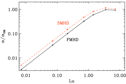
Figure 2: Lu dependence of $\alpha$ for forced magnetic background with Roberts geometry $\mbox{\rm Pr}_{\rm M}=1$, using FMHD with CTFM and (black). Red dashed: SMHD.

In Figure 3 we show the dependence of $\alpha_{xx}$ and $\alpha_{yy}$ on $B_{0}$ for the forced magnetic background with Roberts geometry, $\nu=\eta$ and forcing amplitudes between 0.01 and 100 in units where $\nu=\eta=k_{1}=1$. In these cases, flows are only driven by the Lorentz force. The velocity is generally small compared with $B_{0}/\sqrt{\rho_{\rm ref}}$: it can reach 23% when $B_{0}/\eta k_{1}\sqrt{\rho_{\rm ref}}=1$, but is smaller both for weaker and stronger fields. Note that this test case, in which the turbulent flow is solely induced by the interaction of the imposed field with the magnetic background turbulence $\bm{b}^{(0)}$, is quite different from the shear dynamo case studied in the later parts of the paper, as well as from astrophysical settings in general. The jb, bb, ju, and bu flavors always give the same results for the aligned component $\alpha_{xx}$, also agreeing with those from the imposed field method, but for strong imposed fields (in terms of $B_{0}/b^{(0)}_{\rm rms}$), the perpendicular component, $\alpha_{yy}$, disagrees significantly among the flavors; see the different lines in Figure 3. We note that the discrepancy in $\alpha_{yy}$ is not due to the added compressibility, but was present already in the simplified MHD case of Rheinhardt & Brandenburg (2010), but was not noticed there. As demonstrated in Appendix B, the correctness in $\alpha_{xx}$ is systematic and extends to arbitrary field strengths. Surprisingly, the slope of the quenching characteristic exhibits now power $-5$ while in Rheinhardt & Brandenburg (2010) and Karak et al. (2014) $-4$ had been observed. It is suggestive to attribute this difference to the inclusion of pressure gradient and self-advection.

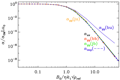
Figure 3: $B_{0}$ dependence of $\alpha$ for the flow-free magnetically forced background with Roberts geometry $\big{(}\bm{0},\bm{b}_{\rm Rob}\big{)}$ and $\mbox{\rm Pr}_{\rm M}=1$ from the CTFM. The results from the imposed-field method are shown by the blue dashed line and agree with all four flavors of the CTFM for $\alpha_{xx}$. The other colored solid lines refer to $\alpha_{yy}$ and departures are seen with the bu flavor. The ju flavor (orange) gives even negative values for $B_{0}/\bm{b}^{(0)}_{\rm rms}\gtrsim 7$, while the bb (red) and jb (green) flavors yield $\alpha_{yy}=\alpha_{xx}$.

3.2 Shear dynamos with SSD magnetic background turbulence

In this section we perform a continuation study of Käpylä et al. (2020), where the SMHD equations were used (governing so-called burgulence) with kinetic and magnetic forcing. Now we turn to full MHD, forced, however, only kinetically with a nonhelical form of the forcing. Hence, in all experiments, we set $\bm{f}_{\rm M}$ to zero. We measure the turbulent transport coefficients from volume averaged quantities, that are, furthermore, averaged over time, neglecting the transients and untrustworthy parts of the time series, as explained in Sect.2.3. The incoherent effects are measured following the same procedure, but rms values are used: $\alpha_{\rm rms}=\big{\langle}\langle{\alpha_{yy}}^{2}\rangle^{1/2}\big{\rangle}_{t}$ and $\eta_{\rm rms}=\big{\langle}\langle{\eta_{yx}}^{2}\rangle^{1/2}\big{\rangle}_{t}$. It should be noted that our values of $\alpha_{\rm rms}$ and $\eta_{\rm rms}$ underestimate the actual ones, which also include the $z$ dependent fluctuations.

In all the simulations performed in this section, we have used the ju variant of the CTFM. This choice is based on test runs with the full shear dynamo setup, see Appendix A, with varying magnetic Prandtl numbers ($\mbox{\rm Pr}_{\rm M}=5\ldots 20$) and $\tilde{S}=-0.2$. These tests revealed that the ju and bb flavors gave results in good agreement both in the kinematic and the nonlinear regime with good stability properties of the test solutions. The jb and bu flavors, however, showed poorer stability properties, hence runs employing them would have required extremely small time steps, rendering them unfeasible. These tests indicate that the nonlinear CTFM (nCTFM) may yield correct results in the case of the shear dynamo as long as the mean field is at most slightly above equipartition with the velocity fluctuations. However, this is no proof of its general applicability.

3.2.1 Vorticity dynamo

For certain values of $\mbox{\rm Pr}_{\rm M}$, namely for 5 and 10, while not for 1 and 20, we see the generation of strong mean flows. In Figure 4 we compare cases with and without rotation from purely hydrodynamical counterparts of our MHD runs. With such experiments we can verify the presence of the mean flows due to a vorticity dynamo and not due to the backreaction of the magnetic field. In the case of $\tilde{\Omega}=0$, hence shear alone (black line in panel (a), and panel (b)), we see the generation of a strong mean flow, which first grows exponentially with a dominating $k_{z}=k_{1}$ mode, and then saturates, exhibiting oscillatory behavior with complicated phase migration. In the MHD runs with TFM the mean flows perturb the system to the extent that the test solutions start to grow super-exponentially. The time step becomes prohibitively small, and no plateaus can be observed anymore in the transport coefficients. Hence, all these TFM measurements have been disregarded.

If a very small amount of rotation is added (panels (c) and (d)), the instability is suppressed, with $u_{{\rm rms}}(t)$ remaining statistically constant throughout the simulation (blue and orange lines in panel (a)). We see, however, that the vertical length scale of the flow is larger in the case of weaker (d) than in the case of stronger rotation (c). This indicates that the $q=-40$ case has still too weak rotation to fully suppress the vorticity dynamo, while $q=-20$ brings the vertical scales close to the forcing scale $k_{\rm f}=10k_{1}$. The presence of weak mean flows for $q=-40$ is also reflected in the slightly larger $u_{{\rm rms}}(t)$ (orange line slightly above the blue one in panel (a)).

We have run CTFM simulations without shear, but with a rotation rate corresponding to $q=-20$, and also with a ten times higher rotation rate; see Figure 5(a)–(d). One can observe that the crucial $\eta_{yx}$ is very similar in the cases with weak rotation, with shear included (orange lines) or excluded (black lines), while all the other $\boldsymbol{\eta}$ components are much more strongly affected. The diagonal components are clearly larger for $\tilde{S}=0$, and $\eta_{xy}$ reverts its sign from strongly positive (with shear) to very low values fluctuating about zero (without shear) From the run with ten times faster rotation (blue lines) we observe that with increasing rotation rate there is a tendency to revert the sign of $\eta_{yx}$ to positive and to increase its magnitude, while reverting $\eta_{xy}$ to negative values, but with weaker magnitude. We conclude that for $q=-20$, the rotation rate is still small enough to not affect the TFM measurements significantly. Hence, we select $q=-20$ as the fiducial parameter for our runs.

We use this setup for all Prandtl numbers above unity, to guarantee that no mean flows disturb the measurements. We note, however, that for $\mbox{\rm Pr}_{\rm M}=20$ the results are nearly identical with and without rotation, indicating that the vorticity dynamo is not active there. This is illustrated in Figure 5(e), where we show the measurements of the $\eta_{yx}$ component with and without rotation, yielding very similar results in the mid-ranges of the resetting intervals. The parameters, varied in the henceforth presented simulations, are the shear rate $\tilde{S}$, the magnetic Prandtl number $\mbox{\rm Pr}_{\rm M}$, and the forcing wavenumber $k_{\rm f}$.

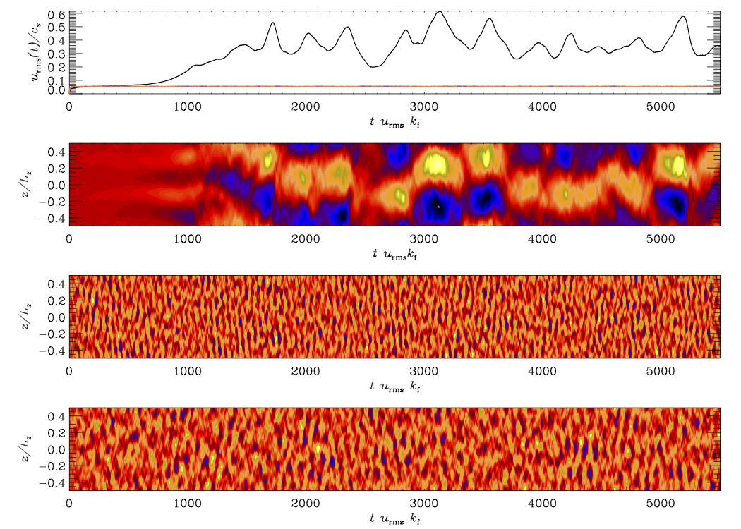
Figure 4: Comparison of the generated mean flows with $\tilde{S}=-0.2$, $\tilde{\Omega}=0$ (black line panel (a); $zt$ diagram in panel (b)), $\tilde{S}=-0.2$, $\tilde{\Omega}=-0.01$ ($q=-20$; blue line in panel (a); (c)), and $\tilde{S}=-0.2$, $\tilde{\Omega}=-0.005$ ($q=-40$; orange line in panel (a); (d)). The uppermost panel shows the time evolution of the volume-averaged rms velocity, $u_{{\rm rms}}(t)$. Colors in the $zt$ diagrams encode $\overline{U}_{y}/c_{\rm s}$ with extrema $\pm 0.7$, $\pm 0.014$, and $\pm 0.022$, in panels (b)–(d), respectively.

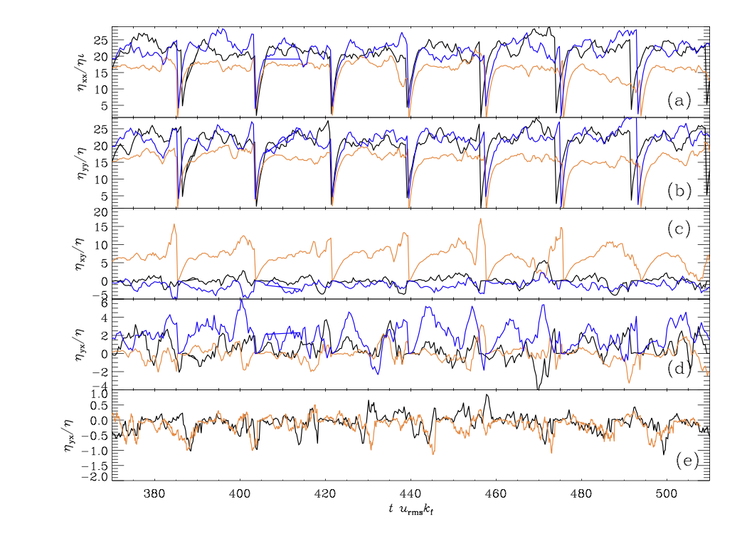
Figure 5: Panels (a)–(d): components of $\boldsymbol{\eta}$, measured with the CTFM and normalized to the microscopic diffusivity $\eta$. Black: $\tilde{S}=0$, $\tilde{\Omega}=-0.01$; blue: $\tilde{S}=0$, ten times stronger rotation ($\tilde{\Omega}=-0.1$); orange: $\tilde{S}=-0.2$, $\tilde{\Omega}=-0.01$ ($q=-20$), all for $\mbox{\rm Pr}_{\rm M}=10$. The time axes have been made to match at $t\,u_{\rm rms}k_{\rm f}=400$ hence orange and blue curves have been introduced with small offsets ($\Delta t\,u_{\rm rms}k_{\rm f}=6$ and 8, respectively). Panel (e): $\eta_{yx}$ from $\mbox{\rm Pr}_{\rm M}=20$ runs with no (black) and weak (orange) rotation ($\tilde{\Omega}=-0.01$, $q=-20$).

Table 1: Summary of the kinematic models with variable $\mbox{\rm Pr}_{\rm M}$, shear rate, and vertical wave number of the test fields.

Run	$\mbox{\rm Pr}_{\rm M}$	$\mbox{\rm Re}_{\rm M}$	$\mbox{\rm Sh}_{\rm K}$	Lu	$\eta_{xx}/\eta$	$\eta_{yy}/\eta$	$\eta_{yx}/\eta$aaa	$\eta_{xy}/\eta$aaa	$\alpha_{\rm rms}/\eta_{t}k_{\rm f}$	$\eta_{\rm rms}/\eta$
S005Pm1k1	1	43	-0.09	13	28.794$\pm$0.322	28.480$\pm$0.227	0.122$\pm$0.296	3.413$\pm$0.413	0.036$\pm$0.012	2.601$\pm$0.381
S005Pm1k2	1	44	-0.09	13	26.183$\pm$0.317	25.134$\pm$0.101	0.468$\pm$1.201	3.839$\pm$1.100	0.025$\pm$0.026	1.282$\pm$1.111
S005Pm1k3	1	43	-0.09	12	21.763$\pm$0.396	22.083$\pm$0.313	-1.707$\pm$1.786	1.786$\pm$0.556	0.035$\pm$0.026	2.241$\pm$2.879
S005Pm20k1	20	34	-0.15	16	11.826$\pm$0.095	12.100$\pm$0.048	0.004$\pm$0.091	1.127$\pm$0.094	0.039$\pm$0.020	0.282$\pm$0.158
S005Pm20k2	20	34	-0.15	16	11.754$\pm$0.097	11.982$\pm$0.051	0.024$\pm$0.080	1.112$\pm$0.101	0.039$\pm$0.021	0.264$\pm$0.182
S005Pm20k3	20	34	-0.15	16	11.667$\pm$0.366	11.749$\pm$0.486	-0.045$\pm$0.043	1.189$\pm$0.078	0.038$\pm$0.024	0.264$\pm$0.189
S01Pm1k1	1	47	-0.16	16	36.436$\pm$0.354	35.382$\pm$0.098	0.435$\pm$0.366	8.707$\pm$0.718	0.029$\pm$0.015	2.839$\pm$1.442
S01Pm1k2	1	48	-0.16	15	33.434$\pm$0.337	31.845$\pm$0.348	0.550$\pm$0.201	6.879$\pm$0.195	0.030$\pm$0.018	2.031$\pm$1.251
S01Pm1k3	1	47	-0.16	16	27.735$\pm$0.264	26.932$\pm$0.335	0.303$\pm$0.217	5.271$\pm$0.162	0.033$\pm$0.019	1.309$\pm$0.683
S01Pm20k1	20	32	-0.30	27	7.811$\pm$0.139	8.389$\pm$0.207	-0.068$\pm$0.066	0.908$\pm$0.166	0.040$\pm$0.018	0.298$\pm$0.283
S01Pm20k2	20	32	-0.30	28	7.678$\pm$0.283	8.151$\pm$0.231	-0.092$\pm$0.064	1.063$\pm$0.149	0.036$\pm$0.020	0.257$\pm$0.112
S01Pm20k3	20	32	-0.30	27	8.272$\pm$0.255	8.766$\pm$0.350	-0.002$\pm$0.033	1.000$\pm$ 0.116	0.033$\pm$0.018	0.227$\pm$0.147
S02Pm1k1	1	66	-0.23	25	70.218$\pm$6.340	65.830$\pm$6.636	0.717$\pm$0.298	32.987$\pm$3.260	0.020$\pm$0.009	4.164$\pm$1.529
S02Pm1k2	1	66	-0.23	25	56.417$\pm$3.857	54.361$\pm$3.352	-0.094$\pm$0.742	22.979$\pm$3.578	0.026$\pm$0.016	2.663$\pm$0.670
S02Pm1k3	1	63	-0.24	24	43.668$\pm$2.935	41.674$\pm$3.695	-0.132$\pm$0.326	14.530$\pm$1.093	0.032$\pm$0.023	1.478$\pm$0.634
S02Pm5k1	5	16	-0.48	17	4.149$\pm$1.205	4.317$\pm$1.542	0.063$\pm$0.071	5.192$\pm$0.215	0.043$\pm$0.017	0.515$\pm$0.143
S02Pm5k2	5	16	-0.48	17	4.765$\pm$0.776	4.576$\pm$0.919	0.019$\pm$0.070	4.993$\pm$0.208	0.036$\pm$0.017	0.370$\pm$0.175
S02Pm5k3	5	16	-0.48	16	5.444$\pm$0.515	5.045$\pm$0.578	0.043$\pm$0.037	3.180$\pm$0.381	0.031$\pm$0.013	0.259$\pm$0.083
S02Pm10k1	10	42	-0.47	45	12.729$\pm$0.989	12.197$\pm$1.002	0.059$\pm$0.109	5.918$\pm$0.179	0.030$\pm$0.011	0.787$\pm$0.475
S02Pm10k2	10	42	-0.47	44	13.203$\pm$0.467	12.637$\pm$0.611	0.139$\pm$0.053	6.440$\pm$0.306	0.027$\pm$0.011	0.542$\pm$0.239
S02Pm10k3	10	42	-0.47	44	13.416$\pm$0.481	12.514$\pm$0.879	0.154$\pm$0.039	5.009$\pm$0.320	0.027$\pm$0.009	0.468$\pm$0.165
S02Pm20k1	20	33	-0.60	45	5.438$\pm$0.278	4.808$\pm$0.138	0.042$\pm$0.103	3.282$\pm$0.738	0.046$\pm$0.019	0.296$\pm$0.061
S02Pm20k2	20	33	-0.60	45	5.503$\pm$0.152	4.900$\pm$0.141	0.064$\pm$0.084	4.462$\pm$0.416	0.045$\pm$0.023	0.269$\pm$0.083
S02Pm20k3 *	20	33	-0.60	44	6.099$\pm$0.140	5.372$\pm$0.232	0.041$\pm$0.013	1.569$\pm$0.784	0.046$\pm$0.013	0.326$\pm$0.084
S02Pm20k3 *	20	33	-0.60	39	6.832$\pm$0.077	6.707$\pm$0.392	-0.020$\pm$0.043	2.255$\pm$0.079	0.035$\pm$0.018	0.224$\pm$0.064
S03Pm20k1	20	35	-0.86	55	5.711$\pm$0.559	5.259$\pm$0.627	-0.043$\pm$0.053	8.692$\pm$0.458	0.039$\pm$0.022	0.240$\pm$0.129
S03Pm20k2	20	35	-0.86	56	5.898$\pm$0.230	5.242$\pm$0.133	0.076$\pm$0.072	7.846$\pm$0.820	0.038$\pm$0.014	0.202$\pm$0.153
S03Pm20k3	20	35	-0.86	56	6.274$\pm$0.255	5.359$\pm$0.161	0.114$\pm$0.052	5.511$\pm$0.480	0.039$\pm$0.022	0.241$\pm$0.129

Note. The run labels are constructed in the following manner: SXXPmYYkZ, where XX indicates the magnitude of the negative $\tilde{S}$, YY the used magnetic Prandtl number $\mbox{\rm Pr}_{\rm M}$, and Z the vertical wave number of the test fields, $k_{B}$. The sets with fixed shear and variable Prandtl number are listed between the two horizontal lines. The forcing wave number is $k_{\rm f}=5k_{1}$ for $\mbox{\rm Pr}_{\rm M}$=1 and $k_{\rm f}=10k_{1}$ for higher $\mbox{\rm Pr}_{\rm M}$. Runs with a star symbol have different SSD solutions.

Run	$\mbox{\rm Re}_{\rm M}$	$\mbox{\rm Sh}_{\rm K}$	Lu	$\eta_{xx}/\eta$	$\eta_{yy}/\eta$	$\eta_{yx}/\eta$aaa	$\eta_{xy}/\eta$aaa	$\alpha_{\rm rms}/\eta_{t}k_{\rm f}$	$\eta_{\rm rms}/\eta$
nS00Pm1	43	0	12	26.491$\pm$0.321	26.919$\pm$0.463	0.094$\pm$0.156	0.233$\pm$0.429	0.044$\pm$0.016	2.873$\pm$0.985
qS00Pm1	43	0	12	27.298$\pm$0.207	26.922$\pm$0.051	0.110$\pm$0.138	-0.159$\pm$0.422	0.045$\pm$0.016	3.353$\pm$1.423
kS005Pm1	43	-0.09	13	28.794$\pm$0.322	28.480$\pm$0.227	0.122$\pm$0.296	3.413$\pm$0.413	0.036$\pm$0.012	2.601$\pm$0.381
nS005Pm1	43	-0.09	13	28.516$\pm$0.549	28.158$\pm$0.502	-0.151$\pm$0.320	4.006$\pm$0.125	0.038$\pm$0.011	2.810$\pm$0.679
qS005Pm1	43	-0.09	13	29.107$\pm$0.377	28.621$\pm$0.517	-0.543$\pm$0.318	4.070$\pm$0.302	0.039$\pm$0.012	2.987$\pm$0.829
kS01Pm1*	47	-0.16	16	36.436$\pm$0.354	35.382$\pm$0.098	0.435$\pm$0.366	8.707$\pm$0.718	0.029$\pm$0.015	2.839$\pm$1.442
nS01Pm1*	43	-0.19	13	27.413$\pm$0.291	27.604$\pm$0.478	0.552$\pm$0.378	6.923$\pm$0.129	0.036$\pm$0.014	2.401$\pm$0.558
qS01Pm1	46	-0.17	18	38.173$\pm$0.653	36.291$\pm$0.830	-1.033$\pm$0.829	11.399$\pm$0.924	0.039$\pm$0.011	5.107$\pm$1.501
kS02Pm1 *	66	-0.23	25	70.218$\pm$6.340	65.830$\pm$6.636	0.717$\pm$0.298	32.987$\pm$3.260	0.020$\pm$0.009	4.164$\pm$1.529
nS02Pm1 *	62	-0.25	28	59.060$\pm$3.234	57.019$\pm$2.562	0.390$\pm$0.554	29.457$\pm$2.578	0.020$\pm$0.011	3.391$\pm$1.806
qS02Pm1	65	-0.24	28	70.091$\pm$0.825	70.265$\pm$0.564	-0.568$\pm$0.277	42.854$\pm$0.917	0.027$\pm$0.008	5.468$\pm$1.317

Table 2: Summary of the $\mbox{\rm Pr}_{\rm M}$=1 runs with varying shear rate.

Note. Runs marked with ‘q’, ‘k’ and ‘n’ have been analyzed with the quasi-kinematic TFM (QKTFM), the kinematic version of the CTFM (no main run), and the CTFM including the main run, respectively. Boldfaced: runs most compatible with Zhou & Blackman (2021). Runs marked with * indicate cases, where the magnetic background turbulence is not statistically similar.

Table 3: Dynamo numbers for the runs with $\mbox{\rm Pr}_{\rm M}$=1 and variable shear rate.

Run	$-\tilde{S}$a	$\!\!\!\!\!{k_{z,\rm kin}}$	$\!\!\!\!\!{k_{z,\rm sat}}$	$\!\!\!\!\!{k_{B}}$	$D_{\eta S}$	$D_{\eta_{\rm rms}S}\!\!\!\!$	$D_{\alpha S}$
		$\!\!\!\!\!{[k_{1}}]$	$\!\!\!\!\!{[k_{1}]}$	$\!\!\!\!\!{[k_{1}]}$
nS00Pm1	0	1	1	1	9$\times 10^{-5}$	0	0
qS00Pm1	0	1	1	1	2$\times 10^{-5}$	0	0
kS005Pm1	0.05	1	1	1	-0.0135	0.2961	0.7048
nS005Pm1	0.05	1	1	1	0.0169	0.3265	0.6812
qS005Pm1	0.05	1	1	1	0.0585	0.3350	0.6829
kS01Pm1	0.1	1	1	1	-0.0609	0.4168	0.8029
nS01Pm1	0.1	1	1	1	-0.1870	0.5908	1.1218
qS01Pm1	0.1	1	1	1	0.1339	0.6988	1.0811
kS02Pm1	0.2	1	1	1	-0.0542	0.3496	0.4357
nS02Pm1	0.2	1	1	1	-0.0076	0.0973	0.0600
qS02Pm1	0.2	1	1	1	0.0401	0.4317	0.5277

Note. The dynamo numbers are calculated based on the wavenumber $k_{z,\rm kin}$ of the fastest growing Fourier mode in the kinematic stage of the LSD. The other wavenumbers are those of the mode dominating in the saturation stage of the mean field, $k_{z,\rm sat}$, and those of the test fields, $k_{B}$. For the kinematic CTFM measurements (label ‘k’, no main run), $k_{z,\rm kin}$ and $k_{z,\rm sat}$ have been taken from the corresponding CTFM run with main run (label ‘n’).

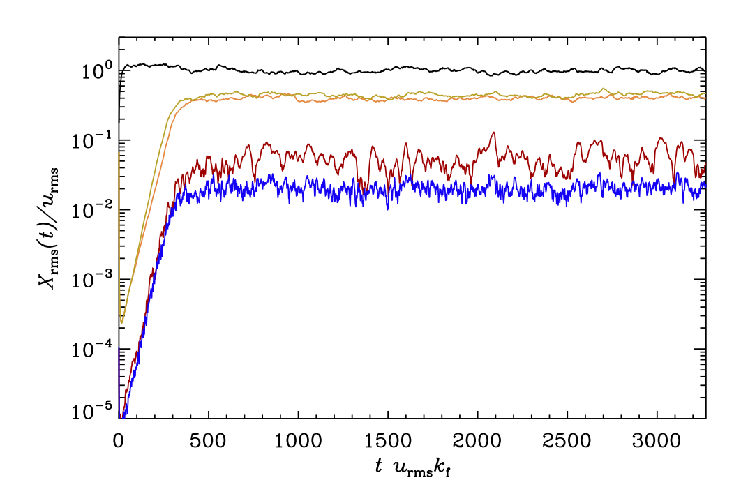
Figure 6: Volume-averaged rms values of the velocity ($u_{{\rm rms}}(t)$, black) and the total magnetic field from the main run ($B_{{\rm rms}}(t)$, yellow), magnetic zero solution ($b_{\rm rms}^{(0)}(t)$, orange), rms values of the mean azimuthal ($\overline{B}_{y,\rm rms}$, red) and radial ($\overline{B}_{x,\rm rms}$, blue) magnetic fields from Run nS02Pm1, all normalized to $u_{\rm rms}$.

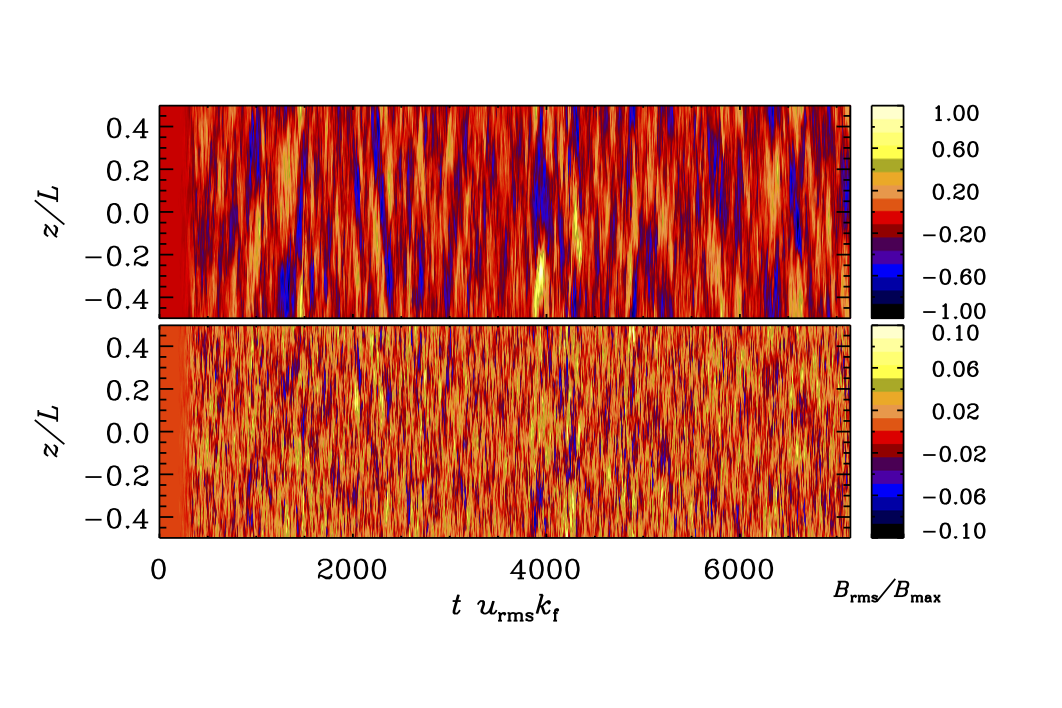
Figure 7: $zt$ diagrams of $\overline{B}_{y}$ (top) and $\overline{B}_{x}$ (bottom) from the main run of qS02Pm1. The main run of nS02Pm1 is identical up to some slight differences due to the difference of time steps.

3.2.2 Kinematic runs

We start by presenting the kinematic CTFM analysis of some shear dynamo models. We stress that this method is generally valid and indispensable in studying the possibility of large-scale dynamo instabilities with magnetic background turbulence $\bm{b}^{(0)}$, which is the main goal of this paper. We vary $\mbox{\rm Pr}_{\rm M}$ and $\mbox{\rm Sh}_{\rm K}$, and study the scale dependence of the turbulent transport coefficients by changing the vertical wavenumber of the test fields, $k_{B}$. We change $\mbox{\rm Pr}_{\rm M}$ by keeping the magnetic resistivity $\eta$ fixed. Hence, the larger $\mbox{\rm Pr}_{\rm M}$, the smaller is Re. The results are summarized in Table 1.

In practice, we ran first only the zero problems until saturation, and then forked new runs with the rest of the test problems turned on. The measurements would not be meaningful before saturation, but this strategy also accelerates the runs. Despite the low Reynolds numbers, the systems are already prone to chaotic behavior, and any small perturbation (such as the random seed of the forcing being initialized differently, or the time step changing slightly when $k_{B}$ is altered) can lead to different small-scale dynamo solutions (for an extreme example, compare the entries marked with a star in Table 1). Hence, for investigating the scale dependence of the coefficients it is desirable to choose runs that have as similar as possible SSD solutions. A general observation is that the stronger the SSD, that is, the stronger the magnetic background turbulence, the weaker are $\eta_{xx}$, $\eta_{yy}$, and $\eta_{xy}$, while $\eta_{yx}$ is always weak and consistent with zero within error bars.

We can also notice that the fluid Reynolds number Re is crucial for the magnitude of the $\boldsymbol{\eta}$ components and their fluctuations, all growing with Re, which is clearly visible when comparing sets with $\mbox{\rm Pr}_{\rm M}$=1 and 20 at the weakest shear. In these, the SSD is weak, and the main effect must come from the flow: For $\mbox{\rm Pr}_{\rm M}=1$, the diagonal components and $\eta_{xy}$ are more than twice, while $\eta_{yx}$ and $\eta_{\rm rms}$ an order of magnitude larger. The magnitude of $\alpha_{\rm rms}/\eta_{\rm t}k_{\rm f}$ remains roughly constant, but note that $\eta_{\rm t}=\left(\eta_{xx}+\eta_{yy}\right)\!/2$.

Continuing with analyzing the sets with weakest shear, $\tilde{S}=-0.05$, that is, $-0.15<\mbox{\rm Sh}_{\rm K}<-0.09$, in the high $\mbox{\rm Pr}_{\rm M}$ case, we find the diagonal $\boldsymbol{\eta}$ components to be roughly equal, i.e. isotropic within error bars. The low $\mbox{\rm Pr}_{\rm M}$ cases with $k_{B}/k_{1}=1$ show no anisotropy either, but this is not equally clear for the higher $k_{B}$ cases, which show weak anisotropy; this could be due to insufficient integration time though, as no significant anisotropy is expected in these weak shear runs without mean magnetic fields and stratification. The high $\mbox{\rm Pr}_{\rm M}$ runs show only weak scale dependence, insignificant within error bars, while the low $\mbox{\rm Pr}_{\rm M}$ runs show a clearly discernible one, such that the diagonal components are reduced when $k_{B}$ is increased. $\eta_{yx}$ is first positive, but turns to negative at the highest $k_{B}$; yet all values are consistent with zero within error bars. The fluctuating quantities show no marked scale dependence at neither Prandtl number.

At moderate shear ($\tilde{S}=-0.1$, resulting in $-0.30<\mbox{\rm Sh}_{\rm K}-0.16$), the diagonal components show a weak anisotropy with both Prandtl numbers investigated. However, for $\mbox{\rm Pr}_{\rm M}=1$, $\eta_{xx}$ is larger than $\eta_{yy}$, while the opposite is true for $\mbox{\rm Pr}_{\rm M}$=20. $\eta_{yx}$ is negative, but consistent with zero within error bars for $\mbox{\rm Pr}_{\rm M}$=20, while significantly positive for $\mbox{\rm Pr}_{\rm M}$=1, for all $k_{B}$. As per the scale dependence, the diagonal $\boldsymbol{\eta}$ components and $\eta_{xy}$ are decreasing with $k_{B}$ for $\mbox{\rm Pr}_{\rm M}=1$, while $\eta_{yx}$ is constant. $\eta_{\rm rms}$ is decreasing with $k_{B}$, too. The trends in the set with $\mbox{\rm Pr}_{\rm M}$=20 are just opposite for the diagonal components and $\eta_{xy}$: they increase with $k_{B}$. These differences must reflect the larger influence of shear on the flow and the stronger SSD generated in the case of $\mbox{\rm Pr}_{\rm M}$=20.

At higher shear ($\tilde{S}=-0.2$, resulting in $-0.60<\mbox{\rm Sh}_{\rm K}<-0.23$), the $\boldsymbol{\eta}$ anisotropy can be observed to get unified: with all the Prandtl numbers studied, $\eta_{xx}$ is systematically larger than $\eta_{yy}$ being statistically significant especially for $\mbox{\rm Pr}_{\rm M}=20$. The diagonal components exhibit only a weak scale dependence in all sets except $\mbox{\rm Pr}_{\rm M}=1$, where a clear decrease as a function of $k_{B}$ is seen. $\eta_{yx}$ has a clear tendency of being positive or consistent with zero. $\eta_{xy}$ is the component showing the most prominent scale dependence with all $\mbox{\rm Pr}_{\rm M}$ used: its magnitude decreases from $k_{B}/k_{1}=1$ to $k_{B}/k_{1}=3$ in all runs, although for $k_{B}/k_{1}=2$, one often finds an increased value in comparison to $k_{B}/k_{1}=1$. Also $\eta_{\rm rms}$ is decreasing as function of $k_{B}$, more prominently so the smaller $\mbox{\rm Pr}_{\rm M}$ is. We also note that with high shear and $k_{B}/k_{1}=1$, $\eta_{xx}$ shows high-frequency oscillations, which vanish at $k_{B}/k_{1}=3$.

Finally, we have run one set with $\tilde{S}=-0.3$, $\mbox{\rm Sh}_{\rm K}\approx-0.86$, and $\mbox{\rm Pr}_{\rm M}$=20. This set has the strongest SSD, but in comparison to the second largest shear rate, $\tilde{S}=-0.2$, the transport coefficients are no longer quenched strongly by it. Otherwise the anisotropy and scale dependence of the measured coefficients is very similar.

To summarize, the main findings in this section are: the SSD quenches the $\boldsymbol{\eta}$ components up to a certain point, while more vigorous kinetic turbulence, quantified by increasing Re, enhances their magnitude. Scale dependence is evident only in runs with high enough Re. Strong shear leads to anisotropy, with $\eta_{xx}>\eta_{yy}$. Kinematic calculations show no evidence for negative values of $\eta_{yx}$ within the studied parameter regime.

3.2.3 Models with Prandtl number of unity

We proceed by discussing runs with $\mbox{\rm Pr}_{\rm M}$ of unity and forcing wavenumber $k_{\rm f}/k_{1}=5$, but the main run with the potential of LSD now included. This choice is motivated by a recent study by Zhou & Blackman (2021), who highlighted weak-shear cases at low to moderate Reynolds numbers and $\mbox{\rm Pr}_{\rm M}=1$ to give rise to a negative $\eta_{yx}$, when measured with the QKTFM. Without further analysis, such a result could be easily interpreted to be (i) contradictory to all previously published numerical results that have not reported negative $\eta_{yx}$ values in incompressible, anelastic, or SMHD, and (ii) favorable for SC effect dynamos.

As in Sect. 3.2.2, we start the measurements only after saturation of the zero problems and proceed until the saturation of the evolving mean fields. Runs of this kind are reported in our tables below with names starting with ‘n’ (nonlinear). The runs starting with ’k’ refer to the corresponding kinematic runs presented in the previous section. We also perform QKTFM measurements for each run (run names starting with ‘q’). In the ‘n’ and ‘q’ cases, we compute the turbulent transport coefficients after the saturation of both types of dynamos (if present).

We begin by presenting results from two runs without shear and rotation employing the CTFM and QKTFM, respectively, and integrated over six thousand turnover times; see the first entries in Table 2. For these setups, a SSD is present, resulting in initial exponential growth of the magnetic field, which then saturates at around 400 turnover times. After that, the magnetic energy stays close to its average saturation value of $\mbox{\rm Lu}\approx 0.25\,\mbox{\rm Re}_{\rm M}$. We see that both methods give consistent results: the diagonal elements are isotropic, i.e., roughly of the same magnitude within error bars, and the off-diagonal elements are consistent with zero. These runs were integrated twice as long as any other run, hence their error bars reflect the minimal level to be achieved with realistic computation times. The agreement of the CTFM and QKTFM is not self-evident: Given the weakness of the SSD, we interpret it as an indication of strong dominance of the contribution $\overline{\bm{u}^{(0)}\times\bm{b}^{(B)}}$ to the mean EMF over $\overline{\bm{u}^{(B)}\times\bm{b}^{(0)}}$; see Sect. 2.2.

By adding shear, we find that the SSD is enhanced in terms of its saturation strength, as indicated by the increasing Lundquist number (Lu) in Table 2. The growth rate also increases somewhat as function of the shear rate; for a typical case see Figure 7 with the largest shear number in this set. For the shear numbers covered, the rms strength of the total magnetic field reaches $\mbox{\rm Lu}\approx 0.42\mbox{\rm Re}_{\rm M}$ at the highest shear. In all cases, the magnetic fields of the zero problem and the main run are of similar strength; correspondingly, the mean fields reach maximally a few percent of the equipartition strength at the highest shear rate. None of the constituents of the magnetic field show significant growth after the SSD has saturated; see Figure 6. Obviously, shear and turbulence have only the capability of generating short-lived large-scale patches in $\overline{B}_{y}$ (see Figure 7), persisting only over a few tens to maximally a couple of hundred turnover times. The timescale of persistence is even shorter in $\overline{B}_{x}$ (maximally a few tens). The wavenumber of these patches is $k_{z}/k_{1}=1$, which is used both as the vertical wavenumber of the test fields in all the measurements, and to compute the dynamo numbers for these runs; see Table 3.

Differences in $\eta_{yx}$ between CTFM and QKTFM start to emerge when shear is increased. As was reported in Sect. 3.2.2, the kinematic CTFM (kCTFM) gives consistently positive values for all values of $\tilde{S}$, although for the weakest shear, $\tilde{S}=-0.05$, the error bars are too large to be certain of the positive sign. Results in close agreement are found beyond kinematics. This is expected as no clear LSD is operational and thus the two versions of the CTFM have to agree. The QKTFM, however, yields negative $\eta_{yx}$ within error bars with all shear numbers investigated. Hence, we can reproduce the results of Zhou & Blackman (2021) of negative $\eta_{yx}$ with the QKTFM, but the results of the CTFM do not lend support to them.

As per the other $\boldsymbol{\eta}$ components, we note that the QKTFM yields larger diagonal components in comparison to the CTFM with main run, especially in the cases with high shear. Both methods give positive values of $\eta_{xy}$, but the values retrieved with the QKTFM are larger than those with CTFM.

We note that in one case, namely with $\tilde{S}=-0.1$, the background turbulence, both in terms of the flow and magnetic field zero solutions $\bm{u}^{(0)}$ and $\bm{b}^{(0)}$, is statistically different between the kinematic and nCTFM runs. We re-iterate that such differences can emerge even in mildly turbulent flows, e.g., due to differences in the time step. Simultaneously, we observe a difference in the measured transport coefficients, such that the diagonal components are larger by about 25% in the kinematic run. Given the weakness of the mean field, we attribute these marked differences to the difference in the background turbulence. In Section 3.2.2, we saw that SSD can diminish the transport coefficients, while a higher level of kinetic turbulence enhances them. In the present case, both effects are present, given the larger $\mbox{\rm Re}_{\rm M}$ and Lu in the kinematic run. This result provides evidence for the enhancing effect by more vigorous kinetic turbulence being stronger than the suppressing effect by the SSD in this shear regime. In the case $\tilde{S}=-0.2$, differences in $\mbox{\rm Re}_{\rm M}$ and Lu can again be observed, again indicative of the background turbulence being different between the kinematic and the nonlinear runs. However, these differences are smaller than for $\tilde{S}=-0.1$, which explains the weaker impact on the coefficients ($\approx$ 15%), but weak mean-field effects cannot be ruled out either.

We also compute the dynamo numbers, following the procedure described earlier, and report them in Table 3. We note that in the shearless case, $D_{\eta S}$ is ideally zero, but not in practice due to limited accuracy of the measurements. With all the shear rates investigated, the dynamo number remain subcritical both with respect to the coherent SC effect and the incoherent ones (for a complete analysis, see Käpylä et al., 2020). This is in perfect agreement with the observation of the mean fields to remain weak with hardly any growth, except for a slight increase in $\overline{B}_{y}$. This is most likely the reason why in the earlier study of Brandenburg et al. (2008a) employing the QKTFM, which concentrated on analyzing the regime with generation of strong large-scale fields, no attention was paid to this parameter regime. We also regard it to be insignificant for the investigation of dynamos in shear flows.

Table 4: Summary of the models with variable $\mbox{\rm Pr}_{\rm M}$ and fixed shear rate.

Run	$\mbox{\rm Pr}_{\rm M}$	$\mbox{\rm Re}_{\rm M}$	$\mbox{\rm Sh}_{\rm K}$	Lu	$\eta_{xx}/\eta$	$\eta_{yy}/\eta$	$\eta_{yx}/\eta$aaa	$\eta_{xy}/\eta$aaa	$\alpha_{\rm rms}/\eta_{t}k_{\rm f}$	$\eta_{\rm rms}/\eta$
kS02Pm5	5	16	-0.48	17	4.765$\pm$0.776	4.576$\pm$0.919	0.019$\pm$0.070	4.993$\pm$0.208	0.036$\pm$0.017	0.370$\pm$0.175
nS02Pm5*	5	16	-0.50	22	4.235$\pm$0.181	4.210$\pm$0.220	0.173$\pm$0.016	0.634$\pm$0.136	0.028$\pm$0.012	0.194$\pm$0.087
qS02Pm5*	5	16	-0.49	18	5.910$\pm$1.429	6.034$\pm$1.388	0.273$\pm$0.125	1.994$\pm$1.447	0.025$\pm$0.009	0.381$\pm$0.315
kS02Pm10	10	42	-0.47	44	13.203$\pm$0.467	12.637$\pm$0.611	0.139$\pm$0.053	6.440$\pm$0.306	0.027$\pm$0.011	0.542$\pm$0.239
nS02Pm10	10	42	-0.47	48	14.832$\pm$1.066	14.923$\pm$1.042	0.501$\pm$0.035	3.710$\pm$1.178	0.026$\pm$0.011	0.659$\pm$0.246
qS02Pm10	10	42	-0.47	49	13.276$\pm$1.528	13.541$\pm$1.641	0.400$\pm$0.077	2.160$\pm$1.844	0.030$\pm$0.011	0.631$\pm$0.376
kS02Pm20	20	33	-0.60	44	6.099$\pm$0.140	5.372$\pm$0.232	0.041$\pm$0.013	1.569$\pm$0.784	0.046$\pm$0.013	0.326$\pm$0.084
nS02Pm20	20	33	-0.60	47	7.356$\pm$0.807	5.608$\pm$0.486	0.000$\pm$0.042	0.874$\pm$0.326	0.041$\pm$0.020	0.202$\pm$0.128
qS02Pm20	20	33	-0.61	47	5.696$\pm$0.462	6.008$\pm$0.528	0.033$\pm$0.021	- 1.017$\pm$0.533	0.045$\pm$0.011	0.228$\pm$0.094

Note. Conventions as in Table 2, except for the star indicating different levels of mean fields present in the models, while the background turbulence is roughly similar. As per the scale of the test fields, in the kinematic CTFM runs we use $k_{B}$ corresponding to the one seen in the main run during the growth phase of the magnetic field, while in the nCTFM ones, $k_{B}/k_{1}=1$ is used in all cases.

Table 5: Dynamo numbers for the models with variable $\mbox{\rm Pr}_{\rm M}$ and fixed shear rate.

Run	$\mbox{\rm Pr}_{\rm M}$	$\!\!\!\!\!{k_{z,\rm kin}}$	$\!\!\!\!\!{k_{z,\rm sat}}$	$\!\!\!\!\!{k_{B}}$	$D_{\eta S}$	$D_{\eta_{\rm rms}S}\!\!\!\!$	$D_{\alpha S}$
		$\!\!\!\!\!{[k_{1}]}$	$\!\!\!\!\!{[k_{1}]}$	$\!\!\!\!\!{[k_{1}]}$
kS02Pm5	5	2	1	2	-0.1137	2.3003	4.2421
nS02Pm5	5	2	1	1	-1.2616	1.4233	2.9659
qS02Pm5	5	2	1	1	-1.1108	1.5666	2.4237
kS02Pm10	10	2	1	2	-0.3556	1.4004	3.4350
nS02Pm10	10	2	1	1	-0.9868	1.3086	2.9487
qS02Pm10	10	2	1	1	-0.7421	1.5195	3.5596
kS02Pm20	20	3	1	3	-0.1981	1.5581	3.1317
nS02Pm20	20	3	1	1	0.0124	0.8021	2.6719
qS02Pm20	20	3	1	1	-0.1564	1.0812	3.2568

Note. Conventions as in Table 3.

3.2.4 Varying Prandtl number and moderate shear

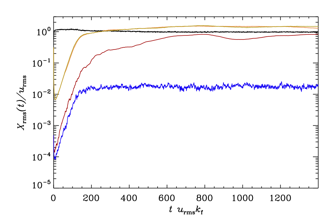
Figure 9: As Figure 6, but for Run nS02Pm20.

Next we map out a part of the parameter space where the generation of significant large-scale magnetic fields occurs. One such regime can be found when $k_{\rm f}/k_{1}=10$ and $\mbox{\rm Pr}_{\rm M}$ is increased, while keeping the shear number $\mbox{\rm Sh}_{\rm K}$ at moderate values. The results are summarized in Table 4. For runs with $5\leq\mbox{\rm Pr}_{\rm M}\leq 20$, we find mean magnetic field configurations closely matching those of (Brandenburg et al., 2008a; Squire & Bhattacharjee, 2015); see Figure 8. In contrast to the weak, incoherent, and short-lived patches seen in Figure 7, the mean azimuthal field grows to near equipartition; see further Figure 9. The $k_{z}/k_{1}=1$ mode emerging in the nonlinear stage exhibits phase coherence nearly throughout the whole 5000 turnover times of the run. Likewise, $\overline{B}_{x}$ shows faint hints of the same pattern, but with a sign opposite to $\overline{B}_{y}$.

The properties of the obtained SSDs and LSDs are as follows: the mean azimuthal field grows always to near equipartition as can be seen from Figure 10. The dynamo growth rates depend on $\mbox{\rm Re}_{\rm M}$, hence the SSD grows slowest for $\mbox{\rm Pr}_{\rm M}=5$, while for $\mbox{\rm Pr}_{\rm M}=10$ and $20$ nearly equally fast, yet with a higher growth rate. For $\mbox{\rm Pr}_{\rm M}=5$, the SSD saturates below equipartition, but very close to it for the higher Prandtl numbers. After saturation of the SSD, mainly $\overline{B}_{y}$ continues to grow. Again, the highest $\mbox{\rm Pr}_{\rm M}$ and $\mbox{\rm Re}_{\rm M}$ cases show the fastest growth, which is, however, distinctly slower than that of the SSD. For $\mbox{\rm Pr}_{\rm M}=5$, the LSD grows the slowest, and, because its SSD’s saturation strength was lower, growth is seen also in $\overline{B}_{x}$. Its growth rate, however, is different from that of $\overline{B}_{y}$, which is somewhat atypical of “standard” dynamos and could be taken indicative of eigenmodes that consist of only one component; see Rheinhardt et al. (2014); Brandenburg & Chen (2020) for examples. However, for an LSD based on the coherent effects alone this can be ruled out here. Eventually, the $\overline{B}_{x}$ components grow equally strong in all cases, while the saturation strength of $\overline{B}_{y}$ is the highest for the highest $\mbox{\rm Pr}_{\rm M}$, but this component undergoes semi-regular oscillations in all the runs. The total magnetic field saturation strength is also increasing with $\mbox{\rm Pr}_{\rm M}$, see the Lundquist numbers in Table 4. Our data also reveals that the saturation values of both $\big{\langle}{\bm{b}^{(0)}}^{2}\big{\rangle}$ and $\big{\langle}{\overline{\bm{B}}}^{2}\big{\rangle}$ grow with $\mbox{\rm Pr}_{\rm M}$. This indicates that a possible reduction of $\big{\langle}\bm{b}^{2}\big{\rangle}$ in comparison to $\big{\langle}{\bm{b}^{(0)}}^{2}\big{\rangle}$, caused by the mean field (quenching), is overcompensated by $\big{\langle}{\overline{\bm{B}}}^{2}\big{\rangle}$ as the total magnetic energy is $\sim\big{\langle}\big{(}\bm{b}+{\overline{\bm{B}}}\big{)}^{2}\big{\rangle}=\big{\langle}{\big{(}\bm{b}^{(0)}+\bm{b}^{(B)}\big{)}}^{2}\big{\rangle}+\big{\langle}{\overline{\bm{B}}}^{2}\big{\rangle}$.

It is very difficult to disentangle the wavenumber of the preferentially growing Fourier mode of the LSD, as the SSD ‘contaminates’ the growth rates: all modes exhibit exponential growth with the same growth rate as long as LSD and SSD grow simultaneously (for a more detailed analysis of a similar system; see Väisälä et al., 2021), and separating the growth rates of these two instabilities is impossible. Hence, we have to rely on the following means of separation: We perform a dedicated set of runs, where we first suppress the mean magnetic field at each time step, while letting the SSD grow until saturation. After that we continue the simulations, but with the mean fields allowed to grow from very small seeds. Now only the eigenmodes of the LSD grow, so we can determine the fastest growing of them and extract its wavenumber $k_{z,{\rm kin}}$. For $\mbox{\rm Pr}_{\rm M}=5$ and 10 we obtain $k_{z}/k_{1}=2$, while $k_{z,{\rm kin}}/k_{1}=3$ for $\mbox{\rm Pr}_{\rm M}=20$. As is evident from Figure 8, in the saturated stage, the mode of wavenumber unity takes over, thus $k_{z,{\rm sat}}/k_{1}=1$. This happens in all LSD–active simulations, as can be seen from Table 5. In this section, we use the former (growth phase) wavenumber in the kinematic CTFM measurements and the latter (nonlinear phase) one in the nonlinear counterparts.

From Table 4, we observe that with none of the employed TFMs the measured $\eta_{yx}$ is negative. Hence, it is unlikely that these dynamos are driven by the coherent magnetic SC effect. We observe that for the highest $\mbox{\rm Pr}_{\rm M}$ investigated, the diagonal components of $\boldsymbol{\eta}$ get significantly anisotropic when measured with the CTFM, such that $\eta_{xx}$ is exceeding $\eta_{yy}$. Since this anisotropy is also recovered with the kinematic version, it cannot solely be due to the mean magnetic field, but must also reflect the growing influence of the shear, given that $\mbox{\rm Sh}_{\rm K}$ is growing with $\mbox{\rm Pr}_{\rm M}$. Contrariwise, we note that the QKTFM does not reveal this anisotropy at all. Moreover, for the highest $\mbox{\rm Pr}_{\rm M}$, the two methods tend to return $\eta_{xy}$ with different sign – still positive for CTFM, but negative for QKTFM. QKTFM also shows opposite anisotropy – $\eta_{yy}$ exceeding $\eta_{xx}$ – albeit insignificant within error bars.

Although the background turbulence of the kinematic and the nonlinear (’n’ and ’q’) runs in this set is satisfactorily similar, the strength of the mean field may differ within the latter ones, depending on, e.g., how long the runs have been integrated, or whether the mean-field was suppressed before the saturation of the SSD or not. Hence, in Table 4, we indicate the runs, where the mean field strength is clearly different with a star, see the $\mbox{\rm Pr}_{\rm M}$=5 set. Here, the kCTFM and nCTFM calculations yield very similar magnitudes of the diagonal $\boldsymbol{\eta}$ components, but QKTFM somewhat larger ones, albeit with large error bars. In the case of $\mbox{\rm Pr}_{\rm M}=10$ and 20, the diagonal $\boldsymbol{\eta}$ components from the nonlinear runs exceed their kinematic counterparts. The fluctuating coefficients are nearly always suppressed in the nonlinear runs.

We can also observe that with the highest $\mbox{\rm Pr}_{\rm M}$, $\eta_{yx}$ is approaching zero with all of the methods used while having been much larger and positive with lower $\mbox{\rm Pr}_{\rm M}$. This could be indicative of a tendency of $\eta_{yx}$ to change sign as $\mbox{\rm Pr}_{\rm M}$ is increased further. We tried to investigate this regime with the CTFM, but observed the test solutions to get unstable, with super-exponential, likely unphysical growth. Accordingly, the measurements become unreliable. Preliminary results from the QKTFM, indeed indicate a sign change of $\eta_{yx}$ to negative, but without the possibility of properly utilizing the CTFM, we leave this to be investigated in forthcoming work.

The kinematic dynamo numbers listed in Table 5, clearly predict positive growth rates for all $\mbox{\rm Pr}_{\rm M}$, as evidenced by the 1D mean-field dynamo model. The nCTFM gives predictions close to marginality, slightly subcritical for $\mbox{\rm Pr}_{\rm M}=5$ and 10, and clearly critical for $\mbox{\rm Pr}_{\rm M}=20$. Those returned by the QKTFM do not predict dynamo action for $\mbox{\rm Pr}_{\rm M}=5$, but for larger $\mbox{\rm Pr}_{\rm M}$, they are clearly supercritical, hence more consistent with the kinematic CTFM kCTFM measurements with $k_{B}$ matching the vertical LSD wavenumber. In all cases in this set, the incoherent effects are sufficient to explain dynamo action, with often slight, but far from fatal inhibition by the coherent effect. We note that for $\mbox{\rm Pr}_{\rm M}=20$, the nCTFM yields positive dynamo numbers $D_{\eta S}$ for the coherent SC effect, but these are clearly below the critical one; moreover, the corresponding $\eta_{yx}$ values turn out to be insignificant within error bars.

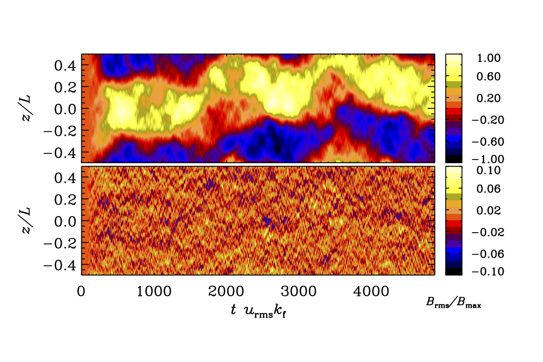
Figure 8: $zt$ diagrams of $\overline{B}_{y}$ (top) and $\overline{B}_{x}$ (bottom) from from the main run of qS02Pm20. The main run of nS02Pm20 is identical up to some slight differences due to the difference of time steps.

Figure 10: Volume-averaged rms values of the total magnetic field from the main run ($B_{{\rm rms}}(t)$, solid), rms values of the mean azimuthal ($\overline{B}_{y,\rm rms}$, dashed), and radial ($\overline{B}_{x,\rm rms}$, dotted) fields from three different runs. Black: qS02Pm5, orange: qS02Pm20, blue: qS02Pm10.

3.2.5 Dependence on the shear rate

Here, we investigate the shear rate dependence of the transport coefficients and the LSD at $\mbox{\rm Pr}_{\rm M}=20$. We perform additional sets of runs with shear rates $\tilde{S}=-0.05,-0.1$, and $-0.3$. As per the efficiency of the LSD, we notice that the strongest mean azimuthal field $\overline{B}_{y}$ in terms of equipartition is obtained with $\tilde{S}=-0.2$. For that value, roughly 70% of the magnetic energy is in the mean field. For $\tilde{S}=-0.1$ the corresponding fraction is 30%, and 55% for $\tilde{S}=-0.3$. Topology and coherence of the mean fields in the nonlinear stage do not change as a function of shear rate: in all runs, we see the dominance of a coherent $k_{z,\rm sat}/k_{1}=1$ mode. The modes growing in the kinematic stage have $k_{z,\rm kin}/k_{1}=2$ for the two lowest shear rates, and $k_{z,\rm kin}/k_{1}=3$ for the two higher ones. By comparing the kCTFM runs with those including the main run, we can also observe that shear enhances the SSD: in the case of the highest shear rate, the values of Lu are larger than in any other set with, at times, even superequipartition $\bm{b}^{(0)}$ for the two highest shear rates. The presence of a more vigorous SSD, however, does not seem to boost the LSD indefinitely with increasing shear, as the fraction of the energy in the mean field is lower in the $\tilde{S}=-0.3$ case than in the $\tilde{S}=-0.2$ one. .

The correctness of the nCTFM with Lu as high as for the highest shear rate, $\tilde{S}=-0.3$, is no longer granted. Hence, for this shear rate, we report measurements with the QKTFM and kCTFM; for all other shear rates we judge the method valid, and report full sets of results. The diagonal components of $\boldsymbol{\eta}$ do not manifest marked anisotropy until $|\tilde{S}|\geq 0.2$, corresponding to $|\mbox{\rm Sh}_{\rm K}|\gtrsim 0.5$. Then, the CTFM indicates $\eta_{xx}>\eta_{yy}$ within error bars, while the QKTFM rather tends to $\eta_{yy}>\eta_{xx}$, yet to be considered insignificant in view of the error bars. QKTFM shows a sign change of $\eta_{xy}$, when $|\tilde{S}|\geq 0.1$, while the CTFM yields positive values. The kinematic variant shows increasing values of $\eta_{xy}$ as function of shear rate, while the nonlinear variant indicates rather decreasing ones. The most marked difference of the methods is seen for $\eta_{yx}$: the kCTFM yields negative, but insignificant values for weak shear, but then significant positive values for strong shear. The nonlinear version, in contrast, shows large positive values with weak shear, and a much reduced value at the highest shear that this method is applicable for. The QKTFM is in rough agreement with the trends of the nCTFM.

The retrieved dynamo numbers (Table 7) indicate slightly subcritical incoherent dynamos for the lowest shear rate, but clearly supercritical incoherent dynamos for all other shear rates. The prediction for the coherent SC-effect dynamo is unfavorable, except for $\tilde{S}=-0.1$, where a positive, yet still subcritical $D_{\eta S}$ is obtained with the kCTFM.

Table 6: Summary of the runs with varying shear rate and $\mbox{\rm Pr}_{\rm M}=20$.

Run	$-S$	$\mbox{\rm Re}_{\rm M}$	$\mbox{\rm Sh}_{\rm K}$	Lu	$\eta_{xx}/\eta$	$\eta_{yy}/\eta$	$\eta_{yx}/\eta$aaa	$\eta_{xy}/\eta$aaa	$\alpha_{\rm rms}/\eta_{t}k_{\rm f}$	$\eta_{\rm rms}/\eta$
kS005Pm20	0.05	34	-0.15	16	11.754$\pm$0.097	11.982$\pm$0.051	0.024$\pm$0.080	1.112$\pm$0.101	0.039$\pm$0.021	0.264$\pm$0.182
nS005Pm20	0.05	34	-0.15	18	12.036$\pm$0.655	12.191$\pm$0.630	0.133$\pm$0.061	1.297$\pm$0.241	0.043$\pm$0.013	0.547$\pm$ 0.278
qS005Pm20	0.05	33	-0.15	20	11.116$\pm$2.280	11.398$\pm$2.113	0.135$\pm$0.089	1.013$\pm$0.677	0.046$\pm$0.020	0.552$\pm$0.354
kS01Pm20	0.1	32	-0.30	28	7.678$\pm$0.283	8.151$\pm$0.231	-0.092$\pm$0.064	1.063$\pm$0.149	0.036$\pm$0.020	0.257$\pm$0.112
nS01Pm20	0.1	33	-0.30	28	9.152$\pm$1.560	9.506$\pm$1.551	0.203$\pm$0.121	1.236$\pm$0.878	0.040$\pm$0.019	0.345$\pm$0.233
qS01Pm20	0.1	32	-0.31	35	6.696$\pm$0.309	7.097$\pm$0.308	0.041$\pm$0.011	-0.426$\pm$0.115	0.050$\pm$0.013	0.297$\pm$0.087
kS02Pm20	0.2	33	-0.60	44	6.099$\pm$0.140	5.372$\pm$0.232	0.041$\pm$0.013	1.569$\pm$0.784	0.046$\pm$0.013	0.326$\pm$0.084
nS02Pm20	0.2	33	-0.60	47	7.356$\pm$0.807	5.608$\pm$0.486	0.000$\pm$0.042	0.874$\pm$0.326	0.041$\pm$0.020	0.202$\pm$0.128
qS02Pm20	0.2	33	-0.61	47	5.696$\pm$0.462	6.008$\pm$0.528	0.033$\pm$0.021	-1.017$\pm$0.533	0.045$\pm$0.011	0.228$\pm$0.094
kS03Pm20	0.3	35	-0.86	56	6.274$\pm$0.255	5.359$\pm$0.161	0.114$\pm$0.052	5.511$\pm$0.480	0.039$\pm$0.022	0.241$\pm$0.129
qS03Pm20	0.3	34	-0.87	60	5.813$\pm$0.311	5.933$\pm$0.333	0.055$\pm$0.022	-0.693$\pm$0.695	0.039$\pm$0.009	0.188$\pm$0.062

Note. Conventions as in Table 2.

Table 7: Dynamo numbers for the models with varying shear rate and $\mbox{\rm Pr}_{\rm M}$=20.

Run	$-S$	$\!\!\!\!\!{k_{z,\rm kin}}$	$\!\!\!\!\!{k_{z,\rm sat}}$	$\!\!\!\!\!{k_{B}}$	$D_{\eta S}$	$D_{\eta_{\rm rms}S}\!\!\!\!$	$D_{\alpha S}$
		$\!\!\!\!\!{[k_{1}}]$	$\!\!\!\!\!{[k_{1}]}$	$\!\!\!\!\!{[k_{1}]}$
kS005Pm20	0.05	2	1	2	-0.0236	0.1952	2.1389
nS005Pm20	0.05	2	1	1	-0.0957	0.3979	2.0790
qS005Pm20	0.05	2	1	1	-0.1110	0.4594	2.4033
kS01Pm20	0.1	2	1	2	0.2891	0.8237	4.5000
nS01Pm20	0.1	2	1	1	-0.4746	0.8095	4.3888
qS01Pm20	0.1	2	1	1	-0.1653	1.1906	6.2656
kS02Pm20	20	3	1	3	-0.1981	1.5581	3.1317
nS02Pm20	20	3	1	1	0.0124	0.8021	2.6719
qS02Pm20	20	3	1	1	-0.1564	1.0812	3.2568
kS03Pm20	0.3	3	1	3	-0.7848	1.4347	2.6384
qS03Pm20	0.3	3	1	1	-0.3848	1.3288	3.4519

Note. Conventions as in Table 3.

4 Conclusions

This work presents the compressible test-field method (CTFM) applicable to full MHD with magnetic background turbulence. We present an extensive set of tests using 2D velocity and magnetic fields of Roberts geometry, for which it has long been known that the quasi-kinematic test-field method (QKTFM) completely fails (giving even the wrong sign of $\alpha$) when a (force-free) magnetic background is forced (Rheinhardt & Brandenburg, 2010). We find agreement in $\boldsymbol{\alpha}$ between the CTFM and the imposed-field method, when the ratio of the (saturated) rms values of the mean field and the magnetic background turbulence, $\overline{B}_{\rm rms}/b^{(0)}_{\rm rms}$ is smaller than $\approx 7$.

Tests with the shear dynamo setup reveal agreement of two different nonlinear flavors of the CTFM up to Lundquist numbers of ${\overline{\bm{B}}}$ of at least 25 while $\overline{B}_{\rm rms}/b^{(0)}_{\rm rms}$ is not exceeding $\approx 0.8$. We also compare with the SMHD approach of our earlier study (Käpylä et al., 2020), neglecting the pressure gradient, and find some mild discrepancies due to the former omission of this term.

We proceed by applying the CTFM to the case of shear dynamos, where our previous study was limited to SMHD with magnetic forcing, and was hence deemed inconclusive. In this work, we use full MHD subject to kinetic non-helical forcing only and moderate $\mbox{\rm Re}_{\rm M}$, yet resulting in vigorous small-scale dynamo (SSD) action. We mostly concentrate on analyzing the kinematic CTFM results due to their general validity, while also presenting results of nonlinear CTFM (nCTFM) within its validity range, and QKTFM ones for comparison. We largely confirm the results of the earlier study, namely, the finding of large-scale dynamos (LSD) excited by the incoherent $\alpha$–shear effect, in the parameter regime of moderate shear numbers ($\mbox{\rm Sh}_{\rm K}\approx-0.3\ldots-0.9$) and magnetic Prandtl numbers $\mbox{\rm Pr}_{\rm M}=5\ldots 20$. With $\mbox{\rm Pr}_{\rm M}=1$, where Zhou & Blackman (2021) measured negative $\eta_{yx}$ (favorable for the coherent SC-effect dynamo) with the QKTFM, we find uninterestingly weak LSD, and the CTFM does not confirm the QKTFM measurements.

Parameter regimes studied in this work are limited to moderate $\mbox{\rm Pr}_{\rm M}$ and $\mbox{\rm Sh}_{\rm K}$. What prevented us from extending our analysis beyond these limits is the aforementioned enhanced instability of the test solutions either in the presence of strong mean flows or very strong magnetic fluctuations. Further studies in this regime might be enabled by using higher resolution and even smaller time steps, greatly increasing the computational challenge, though. Another avenue for future research would be to assess the importance of the density in the Lorentz force, where we have replaced it by a constant reference value. It is conceivable that density variability becomes important at high Mach numbers, which is a regime that has not yet received much attention; but see Rogachevskii et al. (2018) for specific predictions.

Appendix A Shear dynamo test experiments

Given the results from the Roberts flow experiments, where the nCTFM failed to reproduce some of the $\boldsymbol{\alpha}$ coefficients for imposed fields yielding Lundquist numbers above 10, it is important to verify whether the nonlinear method is valid in shear dynamo cases as the generated mean fields at high shear and $\mbox{\rm Pr}_{\rm M}$ reach a strong field regime. In case of the Roberts flow, we had a generally valid method, namely the imposed field one, to compare the CTFM results with, but for determining $\boldsymbol{\eta}$ from a shear dynamo such an alternative does not exist. Hence, we must rely on the comparison of the different flavors of the CTFM, which may provide indication for correctness, but no definite proof. We have re-run many of our shear dynamo runs with the ’bb’ flavor, and show in Figure 11 a comparison with the ju flavor in the nonlinear regime of a typical case with a strong mean field. We plot the time series of the $\boldsymbol{\eta}$ components for seven resetting intervals of the test problems. The diagonal components from both methods agree very well, as can be seen from the top row of Figure 11. The agreement of the off-diagonal components (lower row) is somewhat poorer, but still acceptable. The $\eta_{yx}$ component from the bb flavor shows a slight systematic offset to more positive values, but as this component is small and its time average nearly always consistent with zero within error bars, we conclude that this difference is not significant. The agreement for $\eta_{xy}$ is again rather good.

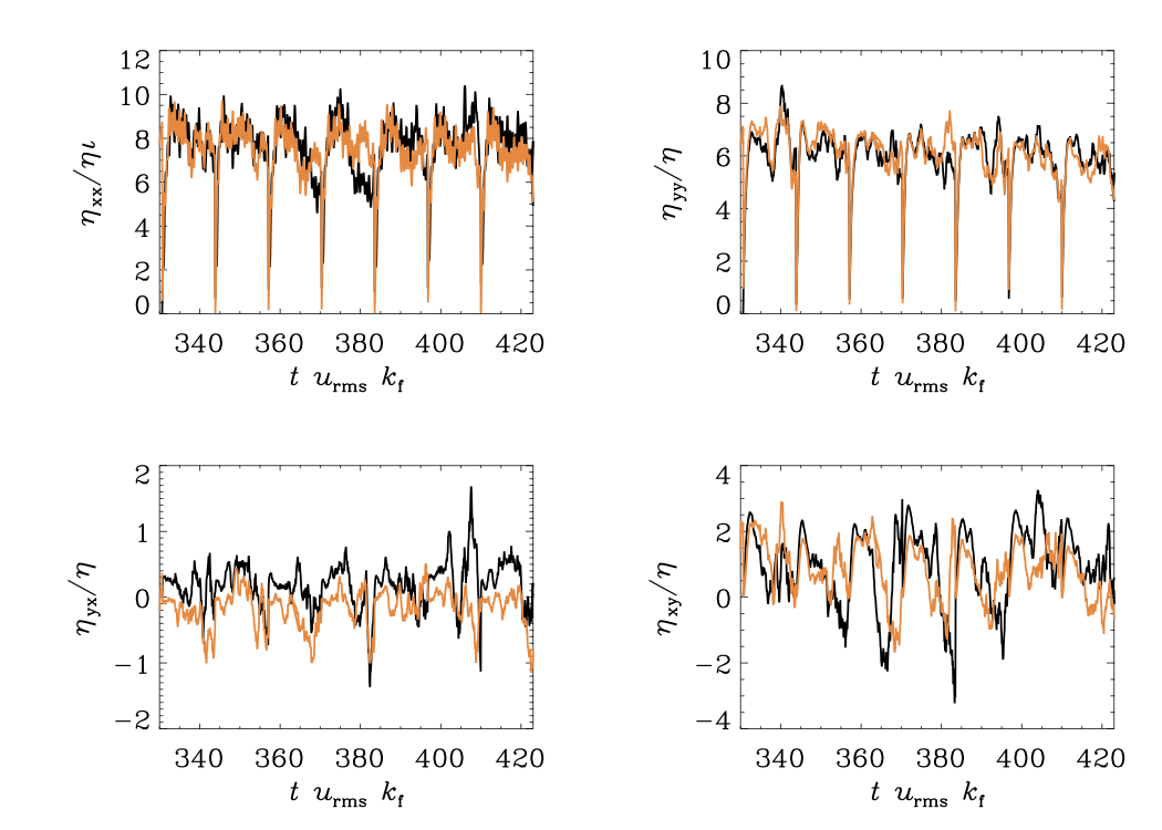
Figure 11: Comparison of the ju (orange lines) and bb (black lines) flavors in the nonlinear stage for $\mbox{\rm Pr}_{\rm M}$=20 and $\tilde{S}$=-0.2 with $\mbox{\rm Lu}\approx$45 based on the total field strength, and $\approx$25 based on the mean-field strength, while $\overline{B}_{\rm rms}/b^{(0)}_{\rm rms}=0.78$

Appendix B Occasional correctness of the nonlinear method

Consider the equations for $\bm{a}^{(B)}$, $\bm{u}^{(B)}$ and $h^{(B)}$ of the main run with imposed uniform field $\bm{B}_{0}$

$${\cal D}{}^{A}\bm{a}^{(B)} = \overline{\bm{U}}\times\bm{b}^{(B)}+\bm{u}\times\bm{B}_{0}+\left(\bm{u}\times\bm{b}^{(B)}+\bm{u}^{(B)}\times\bm{b}^{(0)}\right)^{\prime}+\eta{\bm{\nabla}}^{2}\bm{a}^{(B)},$$ (B1)

$${\cal D}{}^{U}\bm{u}^{(B)} = -{\bm{\nabla}}h^{(B)}+\rho_{\rm ref}^{-1}\left[\bm{j}\times\bm{B}_{0}+\left(\bm{j}\times\bm{b}^{(B)}+\bm{j}^{(B)}\times\bm{b}^{(0)}\right)^{\prime}\right]$$

$$-\overline{\bm{U}}\cdot{\bm{\nabla}}\bm{u}^{(B)}-\bm{u}^{(B)}\cdot{\bm{\nabla}}\overline{\bm{U}}-\left(\bm{u}\cdot{\bm{\nabla}}\bm{u}^{(B)}+\bm{u}^{(B)}\cdot{\bm{\nabla}}\bm{u}^{(0)}\right)^{\prime}$$

$$+\nu\!\left({\bm{\nabla}}^{2}\bm{u}^{(B)}+{\bm{\nabla}}{\bm{\nabla}}\cdot\bm{u}^{(B)}/3\right)+2\nu\left[\overline{\mbox{\boldmath${\mathsf{S}}$}}{}\cdot{\bm{\nabla}}h^{(B)}+\boldsymbol{{\mathsf{s}}}^{(\bm{{B}})}\cdot{\bm{\nabla}}\overline{H}+\left({\sf s}\cdot{\bm{\nabla}}h^{(B)}+\boldsymbol{{\mathsf{s}}}^{(\bm{{B}})}\cdot{\bm{\nabla}}h^{(0)}\right)^{\prime}\right]/c_{\rm s}^{2}$$

$${\cal D}{}h^{(B)} = -\overline{\bm{U}}\cdot{\bm{\nabla}}h^{(B)}-\bm{u}^{(B)}\cdot{\bm{\nabla}}\overline{H}-\left(\bm{u}\cdot{\bm{\nabla}}h^{(B)}+\bm{u}^{(B)}\cdot{\bm{\nabla}}h^{(0)}\right)^{\prime}-c_{\rm s}^{2}{\bm{\nabla}}\cdot\bm{u}^{(B)},$$ (B3)

where the nonlinear terms are here written in the same way as described in Sect. 2.1.4 for the ju flavor of the test problems. Accordingly, the mean EMF is expressed as $\overline{\mbox{\boldmath${\cal E}$}}{}^{(B)}=\overline{\bm{u}\times\bm{b}^{(B)}+\bm{u}^{(B)}\times\bm{b}^{(0)}}$. Note, though, that here these writings represent equivalent rearrangements. Now let us multiply the equations with a constant factor $g$ and redefine the variables as $\bm{a}^{(B)}\coloneqq g\bm{a}^{(B)}$, ${\bm{u}^{(B)}}\coloneqq g\bm{u}^{(B)}$, ${h^{(B)}}\coloneqq gh^{(B)}$, and $\overline{\mbox{\boldmath${\cal E}$}}{}^{(B)}\coloneqq g\overline{\mbox{\boldmath${\cal E}$}}{}^{(B)}$. Of course, for $g\neq 1$, no longer $\bm{a}=\bm{a}^{(0)}+\bm{a}^{(B)}$ etc. holds. We see that the system is now equivalent to that of flavor ju of the test problems with the test field $\bm{B}^{\rm T}$ set equal to the uniform field $g\bm{B}_{0}$ (that is, $\bm{B}^{\rm T}=\bm{B}^{(1)}$ or $\bm{B}^{(3)}$ with $k_{B}=0$ in Equations (25) and (26) ). Inverting the relation $\overline{\cal E}_{i}^{(B)}=\alpha_{ij}B^{(T)}_{j}$ employing $\overline{\mbox{\boldmath${\cal E}$}}{}^{(B)}$ derived from the test solution must hence yield the same result as inverting $\overline{\cal E}_{i}^{(B)}=\alpha_{ij}B_{0,j}$ with $\overline{\mbox{\boldmath${\cal E}$}}{}^{(B)}$ derived from the main run (that is, employing the imposed field method). For any other flavor, the same reasoning can be put forth, so they have to yield identical results. If $\bm{B}_{0}$ is, say, in $x$ direction, the CTFM with $k_{B}=0$ yields thus the correct $\alpha_{ix}$ for arbitrary strengths of the imposed field and hence the nonlinearity. However, $\alpha_{iy}$ cannot correctly be determined as only one of the test fields can be set proportional to $\bm{B}_{0}$.

References

- Brandenburg (2018) Brandenburg, A. 2018, Pencil Code, v2018.12.16, Zenodo, doi: 10.5281/zenodo.2315093
- Brandenburg & Chatterjee (2018) Brandenburg, A., & Chatterjee, P. 2018, Astron. Nachr., 339, 118, doi: 10.1002/asna.201813472
- Brandenburg & Chen (2020) Brandenburg, A., & Chen, L. 2020, J. Plasma Phys., 86, 905860110, doi: 10.1017/S0022377820000082
- Brandenburg et al. (1995) Brandenburg, A., Nordlund, A., Stein, R. F., & Torkelsson, U. 1995, ApJ, 446, 741, doi: 10.1086/175831
- Brandenburg et al. (2008a) Brandenburg, A., Rädler, K. H., Rheinhardt, M., & Käpylä, P. J. 2008a, ApJ, 676, 740, doi: 10.1086/527373
- Brandenburg et al. (2008b) Brandenburg, A., Rädler, K.-H., Rheinhardt, M., & Subramanian, K. 2008b, ApJL, 687, L49, doi: 10.1086/593146
- Brandenburg et al. (2008c) Brandenburg, A., Rädler, K.-H., & Schrinner, M. 2008c, A&A, 482, 739, doi: 10.1051/0004-6361:200809365
- Brandenburg & Sokoloff (2002) Brandenburg, A., & Sokoloff, D. 2002, Geophys. Astrophys. Fluid Dynam., 96, 319, doi: 10.1080/03091920290032974
- Brandenburg et al. (1990) Brandenburg, A., Tuominen, I., Nordlund, A., Pulkkinen, P., & Stein, R. F. 1990, A&A, 232, 277
- Elperin et al. (2003) Elperin, T., Kleeorin, N., & Rogachevskii, I. 2003, PhRvE, 68, 016311, doi: 10.1103/PhysRevE.68.016311
- Hawley (2000) Hawley, J. F. 2000, ApJ, 528, 462, doi: 10.1086/308180
- Hawley et al. (1996) Hawley, J. F., Gammie, C. F., & Balbus, S. A. 1996, ApJ, 464, 690, doi: 10.1086/177356
- Hubbard et al. (2009) Hubbard, A., Del Sordo, F., Käpylä, P. J., & Brandenburg, A. 2009, MNRAS, 398, 1891, doi: 10.1111/j.1365-2966.2009.15108.x
- Käpylä et al. (2018) Käpylä, M. J., Gent, F. A., Väisälä, M. S., & Sarson, G. R. 2018, A&A, 611, A15, doi: 10.1051/0004-6361/201731228
- Käpylä et al. (2020) Käpylä, M. J., Vizoso, J. Á., Rheinhardt, M., Brandenburg, A., & Singh, N. K. 2020, The Astrophysical Journal, 905, 179
- Käpylä et al. (2010) Käpylä, P. J., Korpi, M. J., & Brandenburg, A. 2010, MNRAS, 402, 1458, doi: 10.1111/j.1365-2966.2009.16004.x
- Käpylä et al. (2009) Käpylä, P. J., Mitra, D., & Brandenburg, A. 2009, PhRvE, 79, 016302, doi: 10.1103/PhysRevE.79.016302
- Karak et al. (2014) Karak, B. B., Rheinhardt, M., Brandenburg, A., Käpylä, P. J., & Käpylä, M. J. 2014, ApJ, 795, 16, doi: 10.1088/0004-637X/795/1/16
- Ossendrijver et al. (2001) Ossendrijver, M., Stix, M., & Brandenburg, A. 2001, A&A, 376, 713, doi: 10.1051/0004-6361:20011041
- Pencil Code Collaboration et al. (2021) Pencil Code Collaboration, Brandenburg, A., Johansen, A., et al. 2021, J. Open Source Softw., 6, 2807, doi: 10.21105/joss.02807
- Rheinhardt & Brandenburg (2010) Rheinhardt, M., & Brandenburg, A. 2010, A&A, 520, A28, doi: 10.1051/0004-6361/201014700
- Rheinhardt & Brandenburg (2012) —. 2012, Astron. Nachr., 333, 71, doi: 10.1002/asna.201111625
- Rheinhardt et al. (2014) Rheinhardt, M., Devlen, E., Rädler, K.-H., & Brandenburg, A. 2014, MNRAS, 441, 116, doi: 10.1093/mnras/stu438
- Roberts (1972) Roberts, G. O. 1972, Philosophical Transactions of the Royal Society of London Series A, 271, 411, doi: 10.1098/rsta.1972.0015
- Rogachevskii & Kleeorin (2003) Rogachevskii, I., & Kleeorin, N. 2003, PhRvE, 68, 036301, doi: 10.1103/PhysRevE.68.036301
- Rogachevskii & Kleeorin (2004) —. 2004, PhRvE, 70, 046310, doi: 10.1103/PhysRevE.70.046310
- Rogachevskii et al. (2018) Rogachevskii, I., Kleeorin, N., & Brandenburg, A. 2018, Journal of Plasma Physics, 84, 735840502, doi: 10.1017/S0022377818000983
- Schrinner et al. (2005) Schrinner, M., Rädler, K.-H., Schmitt, D., Rheinhardt, M., & Christensen, U. 2005, Astron. Nachr., 326, 245, doi: 10.1002/asna.200410384
- Schrinner et al. (2007) Schrinner, M., Rädler, K.-H., Schmitt, D., Rheinhardt, M., & Christensen, U. R. 2007, Geophys. Astrophys. Fluid Dynam., 101, 81, doi: 10.1080/03091920701345707
- Shi et al. (2016) Shi, J.-M., Stone, J. M., & Huang, C. X. 2016, MNRAS, 456, 2273, doi: 10.1093/mnras/stv2815
- Simard et al. (2013) Simard, C., Charbonneau, P., & Bouchat, A. 2013, ApJ, 768, 16, doi: 10.1088/0004-637X/768/1/16
- Simard et al. (2016) Simard, C., Charbonneau, P., & Dubé, C. 2016, Advances in Space Research, 58, 1522, doi: 10.1016/j.asr.2016.03.041
- Squire & Bhattacharjee (2015) Squire, J., & Bhattacharjee, A. 2015, ApJ, 813, 52, doi: 10.1088/0004-637X/813/1/52
- Squire & Bhattacharjee (2016) —. 2016, J. Plasma Phys., 82, 535820201, doi: 10.1017/S0022377816000258
- Tilgner & Brandenburg (2008) Tilgner, A., & Brandenburg, A. 2008, MNRAS, 391, 1477, doi: 10.1111/j.1365-2966.2008.14006.x
- Väisälä et al. (2021) Väisälä, M. S., Pekkilä, J., Käpylä, M. J., et al. 2021, ApJ, 907, 83, doi: 10.3847/1538-4357/abceca
- Vishniac & Brandenburg (1997) Vishniac, E. T., & Brandenburg, A. 1997, ApJ, 475, 263, doi: 10.1086/303504
- Warnecke et al. (2018) Warnecke, J., Rheinhardt, M., Tuomisto, S., et al. 2018, A&A, 609, A51, doi: 10.1051/0004-6361/201628136
- Zhou & Blackman (2021) Zhou, H., & Blackman, E. G. 2021, MNRAS, 507, 5732, doi: 10.1093/mnras/stab2469