LGESQL: Line Graph Enhanced Text-to-SQL Model with Mixed Local and Non-Local Relations

Abstract

This work aims to tackle the challenging heterogeneous graph encoding problem in the text-to-SQL task. Previous methods are typically node-centric and merely utilize different weight matrices to parameterize edge types, which 1) ignore the rich semantics embedded in the topological structure of edges, and 2) fail to distinguish local and non-local relations for each node. To this end, we propose a Line Graph Enhanced Text-to-SQL (LGESQL) model to mine the underlying relational features without constructing meta-paths. By virtue of the line graph, messages propagate more efficiently through not only connections between nodes, but also the topology of directed edges. Furthermore, both local and non-local relations are integrated distinctively during the graph iteration. We also design an auxiliary task called graph pruning to improve the discriminative capability of the encoder. Our framework achieves state-of-the-art results ($62.8\%$ with Glove, $72.0\%$ with Electra) on the cross-domain text-to-SQL benchmark Spider at the time of writing.

1 Introduction

The text-to-SQL task Zhong et al. (2017); Xu et al. (2017) aims to convert a natural language question into a SQL query, given the corresponding database schema. It has been widely studied in both academic and industrial communities to build natural language interfaces to databases (NLIDB, Androutsopoulos et al., 1995).

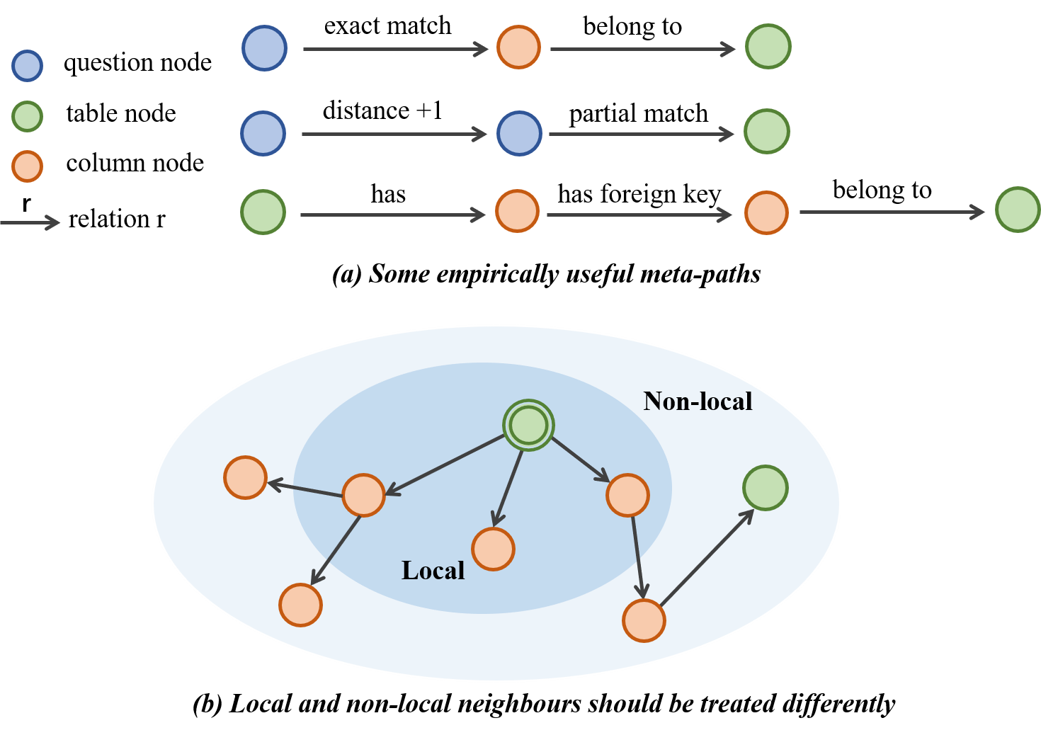
Figure 1: Two limitations if edge features are retrieved from a fixed-size embedding matrix: (a) fail to discover useful meta-paths, and (b) unable to differentiate local and non-local neighbors.

One daunting problem is how to jointly encode the question words and database schema items (including tables and columns), as well as various relations among these heterogeneous inputs. Typically, previous literature utilizes a node-centric graph neural network (GNN, Scarselli et al., 2008) to aggregate information from neighboring nodes. GNNSQL Bogin et al. (2019a) adopts a relational graph convolution network (RGCN, Schlichtkrull et al., 2018) to take into account different edge types between schema items, such as T-Has-C relationship , primary key and foreign key constraints. However, these edge features are directly retrieved from a fixed-size parameter matrix and may suffer from the drawback: unaware of contextualized information, especially the structural topology of edges. Meta-path is defined as a composite relation linking two objects, which can be used to capture multi-hop semantics. For example, in Figure 1(a), relation Q-ExactMatch-C and C-BelongsTo-T can form a 2-hop meta-path indicating that some table $t$ has one column exactly mentioned in the question.

Although RATSQL Wang et al. (2020a) introduces some useful meta-paths such as C-SameTable-C, it treats all relations, either $1$-hop or multi-hop, in the same manner (relative position embedding, Shaw et al., 2018) in a complete graph. Without distinguishing local and non-local neighbors, see Figure 1(b), each node will attend to all the other nodes equally, which may lead to the notorious over-smoothing problem Chen et al. (2020a). Besides, meta-paths are currently constructed by domain experts or explored by breadth-first search Kong et al. (2012). Unfortunately, the number of possible meta-paths increases exponentially with the path length, and selecting the most important subset among them is an NP-complete problem Lao and Cohen (2010).

To address the above limitations, we propose a Line Graph Enhanced Text-to-SQL model (LGESQL), which explicitly considers the topological structure of edges. According to the definition of a line graph Gross and Yellen (2005), we firstly construct an edge-centric graph from the original node-centric graph. These two graphs capture the structural topology of nodes and edges, respectively. Iteratively, each node in either graph gathers information from its neighborhood and incorporates edge features from the dual graph to update its representation. As for the node-centric graph, we combine both local and non-local edge features into the computation. Local edge features denote $1$-hop relations and are dynamically provided by node embeddings in the line graph, while non-local edge features are directly extracted from a parameter matrix. This distinction encourages the model to pay more attention to local edge features while maintaining information from multi-hop neighbors. Additionally, we propose an auxiliary task called graph pruning. It introduces an inductive bias that the heterogeneous graph encoder of text-to-SQL should be intelligent to extract the golden schema items related to the question from the entire database schema graph.

Experimental results on benchmark Spider Yu et al. (2018b) demonstrate that our LGESQL model promotes the exact set match accuracy to $62.8\%$ (with GloVe, Pennington et al. 2014) and $72.0\%$ (with pretrained language model Electra, Clark et al. 2020). Our main contributions are summarized as follows:

• We propose to model the $1$-hop edge features with a line graph in text-to-SQL. Both non-local and local features are integrated during the iteration process of node embeddings.

• We design an auxiliary task called graph pruning, which aims to determine whether each node in the database schema graph is relevant to the given question.

• Empirical results on dataset Spider demonstrate that our model is effective, and we achieve state-of-the-art performances both without and with pre-trained language models.

2 Preliminaries

Problem definition

Given a natural language question $Q=(q_{1},q_{2},\cdots,q_{|Q|})$ with length $|Q|$ and the corresponding database schema $S=T\cup C$, the target is to generate a SQL query $y$. The database schema $S$ contains multiple tables $T=\{t_{1},t_{2},\cdots\}$ and columns $C=\{c_{1}^{t_{1}},c_{2}^{t_{1}},\cdots,c_{1}^{t_{2}},c_{2}^{t_{2}},\cdots\}$. Each table $t_{i}$ is described by its name and is further composed of several words $(t_{i1},t_{i2},\cdots)$. Similarly, we use word phrase $(c_{j1}^{t_{i}},c_{j2}^{t_{i}},\cdots)$ to represent column $c_{j}^{t_{i}}\in t_{i}$. Besides, each column $c_{j}^{t_{i}}$ also has a type field $c_{j0}^{t_{i}}$ to constrain its cell values (e.g. Text and Number).

The entire input node-centric heterogeneous graph $G^{n}=(V^{n},R^{n})$ consists of all three types of nodes mentioned above, that is $V^{n}=Q\cup T\cup C$ with the number of nodes $|V^{n}|=|Q|+|T|+|C|$, where $|T|$ and $|C|$ are the number of tables and columns respectively.

Meta-path

As shown in Figure 1(a), a meta-path represents a path $\tau_{1}\overset{r_{1}}{\rightarrow}\tau_{2}\overset{r_{2}}{\rightarrow}\cdots\overset{r_{l}}{\rightarrow}\tau_{l+1}$, where the target vertex type of previous relation $r_{i-1}$ equals to the source vertex type $\tau_{i}$ of the current relation $r_{i}$. It describes a composite relation $r=r_{1}\circ r_{2}\cdots\circ r_{l}$ between nodes with type $\tau_{1}$ and $\tau_{l+1}$. In this work, $\tau_{i}\in\{\textsc{Question,Table,Column}\}$. Throughout our discussion, we use the term local to denote relations with path length $1$, while non-local relations refer to meta-paths longer than $1$. The relational adjacency matrix $R^{n}$ contains both local and non-local relations, see Appendix A for enumeration.

Line Graph

Each vertex $v_{i}^{e},i=1,2,\cdots,|V^{e}|$ in the line graph $G^{e}=(V^{e},R^{e})$ can be uniquely mapped to a directed edge $r_{st}^{n}\in R^{n}$, or $v_{s}^{n}\rightarrow v_{t}^{n}$, in the original node-centric graph $G^{n}=(V^{n},R^{n})$. Function $f$ maps the source and target node index tuple $(s,t)$ into the “edge” index $i=f(s,t)$ in $G^{e}$. The reverse mapping is $f^{\textrm{-}1}$. In the line graph $G^{e}$, a directed edge $r^{e}_{ij}\in R^{e}$ exists from node $v^{e}_{i}$ to $v^{e}_{j}$, iff the target node of edge $r^{n}_{f^{\textrm{-}1}(i)}$ and the source node of edge $r^{n}_{f^{\textrm{-}1}(j)}$ in $G^{n}$ are exactly the same node. Actually, $r^{e}_{ij}$ captures the information flow in meta-path $r^{n}_{f^{\textrm{-}1}(i)}\circ r^{n}_{f^{\textrm{-}1}(j)}$. We prevent back-tracking cases where two reverse edges will not be connected in $G^{e}$, illustrated in Figure 2.

We only utilize local relations in $R^{n}$ as the node set $V^{e}$ to avoid creating too many nodes in the line graph $G^{e}$. Symmetrically, each edge in $R^{e}$ can be uniquely identified by the node in $V^{n}$. For example, in the upper right part of Figure 2, the edge between nodes “e1” and “e2” in the line graph can be represented by the middle node with double solid borderlines in the original graph.

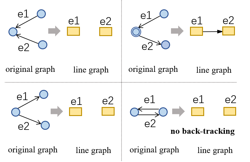
Figure 2: Construction of a line graph. For clarity, we simplify the notation of edges.

3 Method

After constructing the line graph, we utilize the classic encoder-decoder architecture Sutskever et al. (2014); Bahdanau et al. (2015) as the backbone of our model. LGESQL consists of three parts: a graph input module, a line graph enhanced hidden module, and a graph output module (see Figure 3 for an overview). The first two modules aim to map the input heterogeneous graph $G^{n}$ into node embeddings $\mathbf{X}\in\mathbb{R}^{|V^{n}|\times d}$, where $d$ is the graph hidden size. The graph output module retrieves and transforms $\mathbf{X}$ into the target SQL query $y$.

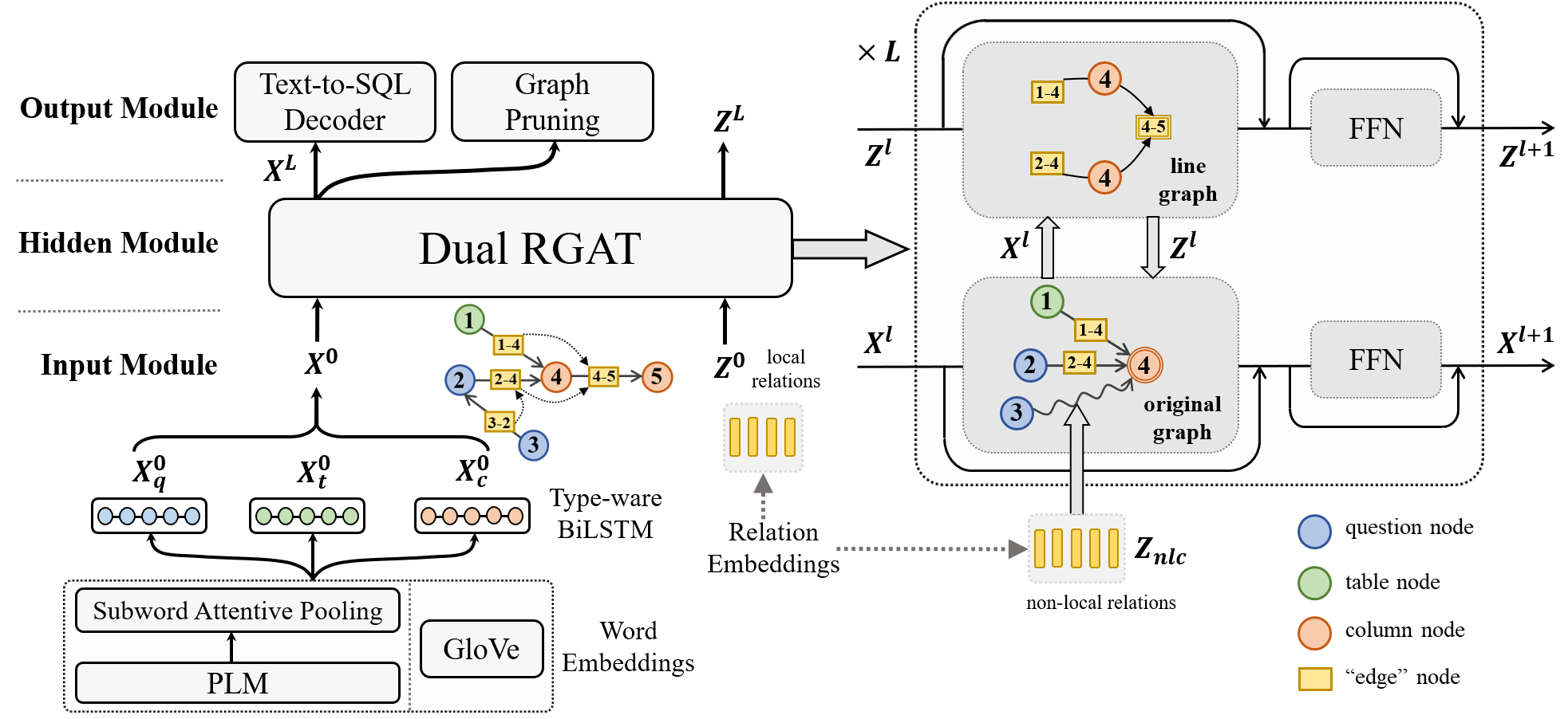
Figure 3: The overall model architecture. We use bidirectional edges in practice but only draw unidirectional edges for better understanding. In the Dual RGAT module, we take the node with index $4$ and the edge with label $4\textrm{-}5$ as the main focuses.

3.1 Graph Input Module

This module aims to provide the initial embeddings for both nodes and edges. Initial local edge features $\mathbf{Z}^{0}\in\mathbb{R}^{|V^{e}|\times d}$ and non-local edge features $\mathbf{Z}_{nlc}\in\mathbb{R}^{(|R^{n}|-|V^{e}|)\times d}$ are directly retrieved from a parameter matrix. For nodes, we can obtain their representations from either word vectors Glove Pennington et al. (2014) or a pre-trained language model (PLM) such as Bert Devlin et al. (2019).

GloVe

Each word $q_{i}$ in the question $Q$ or schema item $t_{i}\in T$ or $c_{j}^{t_{i}}\in C$ can be initialized by looking up the embedding dictionary without considering the context. Then, these vectors are passed into three type-ware bidirectional LSTMs (BiLSTM, Hochreiter and Schmidhuber, 1997) respectively to attain contextual information. We concatenate the forward and backward hidden states for each question word $q_{i}$ as the graph input $\mathbf{x}^{0}_{q_{i}}$. As for table $t_{i}$, after feeding $(t_{i0},t_{i1},t_{i2},\cdots)$ into the BiLSTM (special type $t_{i0}=``table",\forall i$), we concatenate the last hidden states in both directions as the graph input $\mathbf{x}^{0}_{t_{i}}$ (similarly for column $c_{j}^{t_{i}}$). These node representations are stacked together to form the initial node embeddings matrix $\mathbf{X}^{0}\in\mathbb{R}^{|V^{n}|\times d}$.

PLM

Firstly, we flatten all question words and schema items into a sequence, where columns belong to the same table are clustered together : [CLS]$q_{1}q_{2}\cdots q_{|Q|}$[SEP]$t_{10}t_{1}c_{10}^{t_{1}}c_{1}^{t_{1}}c_{20}^{t_{1}}c_{2}^{t_{1}}\cdots$ $t_{20}t_{2}c_{10}^{t_{2}}c_{1}^{t_{2}}c_{20}^{t_{2}}c_{2}^{t_{2}}\cdots$[SEP]. The type information $t_{i0}$ or $c_{j0}^{t_{i}}$ is inserted before each schema item. Since each word $w$ is tokenized into sub-words, we append a subword attentive pooling layer after PLM to obtain word-level representations. Concretely, given the output sequence of subword features $\mathbf{w}^{s}_{1},\mathbf{w}^{s}_{2},\cdots,\mathbf{w}^{s}_{|w|}$ for each subword $w^{s}_{i}$ in $w$, the word-level representation $\mathbf{w}$ is 

$$a_{i}= \text{softmax}_{i}\ \text{tanh}(\mathbf{w}^{s}_{i}\mathbf{W}_{s})\mathbf{v}_{s}^{\mathrm{T}},$$

$$\mathbf{w}= \sum_{i}a_{i}\mathbf{w}^{s}_{i},$$

where $\mathbf{v}_{s}$ and $\mathbf{W}_{s}$ are trainable parameters. After obtaining the word vectors, we also feed them into three BiLSTMs according to the node types and get the graph inputs $\mathbf{X}^{0}$ for all nodes.

3.2 Line Graph Enhanced Hidden Module

It contains a stack of $L$ dual relational graph attention network (Dual RGAT) layers. In each layer $l$, two RGATs Wang et al. (2020b) capture the structure of the original graph and line graph, respectively. Node embeddings in one graph play the role of edge features in another graph. For example, the edge features used in graph $G^{n}$ are provided by the node embeddings in graph $G^{e}$.

We use $\mathbf{X}^{l}\in\mathbb{R}^{|V^{n}|\times d}$ to denote the input node embedding matrix of graph $G^{n}$ in the $l$-th layer, $l\in\{0,1,\cdots,L-1\}$. As for each specific node $v^{n}_{i}\in V^{n}$, we use $\mathbf{x}^{l}_{i}$. Similarly, matrix $\mathbf{Z}^{l}\in\mathbb{R}^{|V^{e}|\times d}$ and vector $\mathbf{z}^{l}_{i}$ are used to denote node embeddings in the line graph. Following RATSQL Wang et al. (2020a), we use multi-head scaled dot-product Vaswani et al. (2017) to calculate the attention weights. For brevity, we formulate the entire computation in one layer as two basic modules:

$$\mathbf{X}^{l+1}= \text{RGAT}^{n}(\mathbf{X}^{l},[\mathbf{Z}^{l};\mathbf{Z}_{nlc}],G^{n}),$$

$$\mathbf{Z}^{l+1}= \text{RGAT}^{e}(\mathbf{Z}^{l},\mathbf{X}^{l},G^{e}),$$

where $\mathbf{Z}_{nlc}$ is the aforementioned non-local edge features in the original graph $G^{n}$.

3.2.1 RGAT for the Original Graph

Given the node-centric graph $G^{n}$, the output representation $\mathbf{x}^{l+1}_{i}$ of the $l$-th layer is computed by

$$\tilde{\alpha}_{ji}^{h}= (\mathbf{x}^{l}_{i}\mathbf{W}^{h}_{q})(\mathbf{x}^{l}_{j}\mathbf{W}^{h}_{k}+[\psi(r_{ji}^{n})]^{H}_{h})^{\mathrm{T}},$$

$$\alpha_{ji}^{h}= \text{softmax}_{j}(\tilde{\alpha}_{ji}^{h}/\sqrt{d/H}),$$

$$\tilde{\mathbf{x}}^{l}_{i}= \bigparallel_{h=1}^{H}\sum_{v_{j}^{n}\in\mathcal{N}^{n}_{i}}\alpha_{ji}^{h}(\mathbf{x}^{l}_{j}\mathbf{W}^{h}_{v}+[\psi(r_{ji}^{n})]^{H}_{h}),$$

$$\tilde{\mathbf{x}}^{l+1}_{i}= \text{LayerNorm}(\mathbf{x}^{l}_{i}+\tilde{\mathbf{x}}^{l}_{i}\mathbf{W}_{o}),$$

$$\mathbf{x}^{l+1}_{i}= \text{LayerNorm}(\tilde{\mathbf{x}}^{l+1}_{i}+\text{FFN}(\tilde{\mathbf{x}}^{l+1}_{i})),$$

where $\parallel$ represents vector concatenation, matrices $\mathbf{W}_{q}^{h},\mathbf{W}_{k}^{h},\mathbf{W}_{v}^{h}\in\mathbb{R}^{d\times d/H},\mathbf{W}_{o}\in\mathbb{R}^{d\times d}$ are trainable parameters, $H$ is the number of heads and $\text{FFN}(\cdot)$ denotes a feedforward neural network. $\mathcal{N}^{n}_{i}$ represents the receptive field of node $v^{n}_{i}$ and function $\psi(r_{ji}^{n})$ returns a $d$-dim feature vector of relation $r_{ji}^{n}$. Operator $[\cdot]_{h}^{H}$ first evenly splits the vector into $H$ parts and returns the $h$-th partition. Since there are two genres of relations (local and non-local), we design two schemes to integrate them:

Mixed Static and Dynamic Embeddings

If $r_{ji}^{n}$ is a local relation, $\psi(r_{ji}^{n})$ returns the node embedding $\mathbf{z}^{l}_{f(j,i)}$ from the line graph. Otherwise, $\psi(r_{ji}^{n})$ directly retrieves the vector from the non-local embedding matrix $\mathbf{Z}_{nlc}$, see Figure 4. The neighborhood function $\mathcal{N}^{n}_{i}$ for node $v^{n}_{i}$ returns the entire node set $V^{n}$ and is shared across different heads.

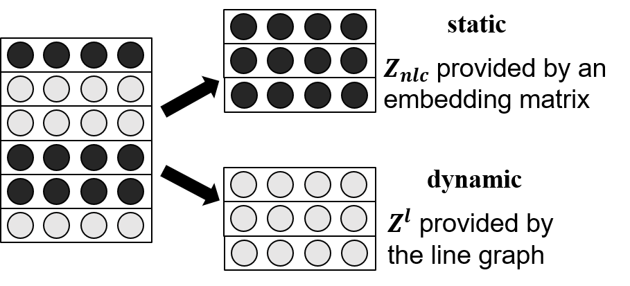
Figure 4: Mixed static and dynamic embeddings.

Multi-head Multi-view Concatenation

An alternative is to split the muli-head attention module into two parts. In half of the heads, the neighborhood function $\mathcal{N}^{n}_{i}$ of node $v^{n}_{i}$ only contains nodes that are reachable within $1$-hop. In this case, $\psi(r_{ji}^{n})$ returns the layer-wise updated feature $\mathbf{z}^{l}_{f(j,i)}$ from $\mathbf{Z}^{l}$. In the other heads, each node has access to both local and non-local neighbors, and $\psi(\cdot)$ always returns static entries in the embedding matrix $\mathbf{Z}_{nlc}\cup\mathbf{Z}^{0}$, see Figure 5 for illustration.

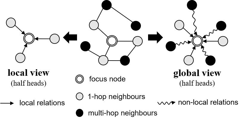
Figure 5: Multi-head multi-view concatenation.

In either scheme, the RGAT module treats local and non-local relations differently and relatively manipulates the local edge features more carefully.

3.2.2 RGAT for the Line Graph

Symmetrically, given edge-centric graph $G^{e}$, the updated node representation $\mathbf{z}^{l+1}_{i}$ from $\mathbf{z}^{l}_{i}$ is calculated similarly with little modifications:

$$\tilde{\beta}_{ji}^{h}= (\mathbf{z}^{l}_{i}\mathbf{U}^{h}_{q}+[\phi(r_{ji}^{e})]^{H}_{h})(\mathbf{z}^{l}_{j}\mathbf{U}^{h}_{k})^{\mathrm{T}},$$

$$\beta_{ji}^{h}= \text{softmax}_{j}(\tilde{\beta}_{ji}^{h}/\sqrt{d/H}),$$

$$\tilde{\mathbf{z}}^{l}_{i}= \bigparallel_{h=1}^{H}\sum_{v_{j}^{e}\in\mathcal{N}^{e}_{i}}\beta_{ji}^{h}(\mathbf{z}^{l}_{j}\mathbf{U}^{h}_{v}+[\phi(r_{ji}^{e})]^{H}_{h}),$$

$$\tilde{\mathbf{z}}^{l+1}_{i}= \text{LayerNorm}(\mathbf{z}^{l}_{i}+\tilde{\mathbf{z}}^{l}_{i}\mathbf{U}_{o}),$$

$$\mathbf{z}^{l+1}_{i}= \text{LayerNorm}(\tilde{\mathbf{z}}^{l+1}_{i}+\text{FFN}(\tilde{\mathbf{z}}^{l+1}_{i})).$$

Here $\phi(r_{ji}^{e})$ returns the feature vector of relation $r_{ji}^{e}$ in $G^{e}$. Since we only consider local relations in the line graph, $\mathcal{N}^{e}_{i}$ only includes $1$-hop neighbous and $\phi(r_{ji}^{e})$ equals to the source node embedding in $\mathbf{X}^{l}$ of edge $v_{i}^{e}$. Attention that the relational feature is added on the “query” side instead of the “key” side when computing attention logits $\tilde{\beta}_{ji}^{h}$ cause it is irrelevant to the incoming edges. For example, in Figure 3, the connecting nodes of two edge pairs $(1\textrm{-}4,4\textrm{-}5)$ and $(2\textrm{-}4,4\textrm{-}5)$ are the same node with index $4$. $\mathbf{U}_{q}^{h},\mathbf{U}_{k}^{h},\mathbf{U}_{v}^{h}\in\mathbb{R}^{d\times d/H},\mathbf{U}_{o}\in\mathbb{R}^{d\times d}$ are trainable parameters.

The output matrices of the final layer $L$ are the desired outputs of the encoder: $\mathbf{X}=\mathbf{X}^{L},\mathbf{Z}=\mathbf{Z}^{L}$.

3.3 Graph Output Module

This module includes two tasks: one decoder for the main focus text-to-SQL and the other one to perform an auxiliary task called graph pruning. We use the subscript to denote the collection of node embeddings with a specific type, e.g., $\mathbf{X}_{q}$ is the matrix of all question node embeddings.

3.3.1 Text-to-SQL Decoder

We adopt the grammar-based syntactic neural decoder Yin and Neubig (2017) to generate the abstract syntax tree (AST) of the target query $y$ in depth-first-search order. The output at each decoding timestep is either 1) an ApplyRule action that expands the current non-terminal node in the partially generated AST, or 2) SelectTable or SelectColumn action that chooses one schema item $\mathbf{x}_{s_{i}}$ from the encoded memory $\mathbf{X}_{s}=\mathbf{X}_{t}\cup\mathbf{X}_{c}$. Mathematically, $P(y|\mathbf{X})=\prod_{j}P(a_{j}|a_{<j},\mathbf{X})$, where $a_{j}$ is the action at the $j$-th timestep. For more implementation details, see Appendix B.

3.3.2 Graph Pruning

We hypothesize that a powerful encoder should distinguish irrelevant schema items from golden schema items used in the target query. In Figure 6, the question-oriented schema sub-graph (above the shadow region) can be easily extracted. The intent $c2$ and the constraint $c5$ are usually explicitly mentioned in the question, identified by dot-product attention mechanism or schema linking. The linking nodes such as $t1,c3,c4,t2$ can be inferred by the $1$-hop connections of the schema graph to form a connected component. To introduce this inductive bias, we design an auxiliary task that aims to classify each schema node $s_{i}\in S=T\cup C$ based on its relevance with the question and the sparse structure of the schema graph.

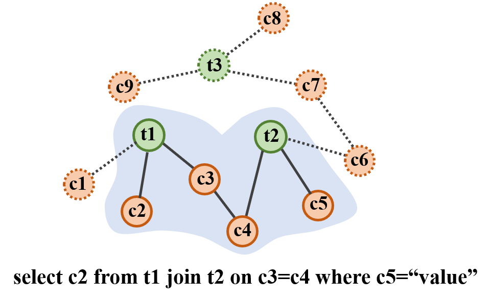
Figure 6: A delexicalized example of graph pruning. Circles with dashed borderlines are irrelevant schema items, thus labeled with $0$.

Firstly, we compute the context vector $\tilde{\mathbf{x}}_{s_{i}}$ from the question node embeddings $\mathbf{X}_{q}$ for each schema node $s_{i}$ via multi-head attention.

$$\gamma^{h}_{ji}= \text{softmax}_{j}\frac{(\mathbf{x}_{s_{i}}\mathbf{W}_{sq}^{h})(\mathbf{x}_{q_{j}}\mathbf{W}_{sk}^{h})^{\mathrm{T}}}{\sqrt{d/H}},$$

$$\tilde{\mathbf{x}}_{s_{i}}= (\bigparallel_{h=1}^{H}\sum_{j}\gamma^{h}_{ji}\mathbf{x}_{q_{j}}\mathbf{W}^{h}_{sv})\mathbf{W}_{so},$$

where $\mathbf{W}_{sq}^{h},\mathbf{W}_{sk}^{h},\mathbf{W}^{h}_{sv}\in\mathbb{R}^{d\times d/H}$ and $\mathbf{W}_{so}\in\mathbb{R}^{d\times d}$ are network parameters. Then, a biaffine Dozat and Manning (2017) binary classifier is used to determine whether the compressed context vector $\tilde{\mathbf{x}}_{s_{i}}$ and the schema node embedding $\mathbf{x}_{s_{i}}$ are correlated.

$$\text{Biaffine}(\mathbf{x}_{1},\mathbf{x}_{2})= \mathbf{x}_{1}\mathbf{U}_{s}\mathbf{x}_{2}^{\mathrm{T}}+[\mathbf{x}_{1};\mathbf{x}_{2}]\mathbf{W}_{s}+b_{s},$$

$$P^{\text{gp}}(y_{s_{i}}|\mathbf{x}_{s_{i}},\mathbf{X}_{q})= \sigma(\text{Biaffine}(\mathbf{x}_{s_{i}},\tilde{\mathbf{x}}_{s_{i}})).$$

The ground truth label $y_{s_{i}}^{g}$ of a schema item is $1$ iff $s_{i}$ appears in the target SQL query. The training object can be formulated as

$$\mathcal{L}_{gp}=-\sum_{s_{i}}[y_{s_{i}}^{g}\log P^{gp}(y_{s_{i}}|\mathbf{x}_{s_{i}},\mathbf{X}_{q})\\ +(1-y_{s_{i}}^{g})\log(1-P^{gp}(y_{s_{i}}|\mathbf{x}_{s_{i}},\mathbf{X}_{q}))].$$

This auxiliary task is combined with the main text-to-SQL task in a multitasking way. Similar ideas Bogin et al. (2019b); Yu et al. (2020) and other association schemes are discussed in Appendix C.

4 Experiments

In this section, we evaluate our LGESQL model in different settings. Codes are public available .

4.1 Experiment Setup

Dataset

Spider Yu et al. (2018b) is a large-scale cross-domain zero-shot text-to-SQL benchmark . It contains $8659$ training examples across $146$ databases in total, and covers several domains from other datasets such as Restaurants Popescu et al. (2003), GeoQuery Zelle and Mooney (1996), Scholar Iyer et al. (2017), Academic Li and Jagadish (2014), Yelp and IMDB Yaghmazadeh et al. (2017) datasets. The detailed statistics are shown in Table 1. We follow the common practice to report the exact set match accuracy on the validation and test dataset. The test dataset contains $2147$ samples with $40$ unseen databases but is not public available. We submit our model to the organizer of the challenge for evaluation.

	Train	Dev
# of samples	$8659$	$1034$
# of databases	$146$	$20$
Avg # of question nodes	$13.4$	$13.8$
Avg # of table nodes	$6.6$	$4.5$
Avg # of column nodes	$33.1$	$25.8$
Avg # of nodes	$53.1$	$44.1$
Avg # of actions	$16.3$	$15.4$

Table 1: Statistics for dataset Spider. The action sequence is created with our designed grammar.

Implementations

We preprocess the questions, table names, and column names with toolkit Stanza Qi et al. (2020) for tokenization and lemmatization. Our model is implemented with Pytorch Paszke et al. (2019), and the original and line graphs are constructed with library DGL Wang et al. (2019a). Within the encoder, we use GloVe Pennington et al. (2014) word embeddings with dimension $300$ or pretrained language models (PLMs), Bert Devlin et al. (2019) or Electra (Clark et al., 2020), to leverage contextual information. With GloVe, embeddings of the most frequent $50$ words in the training set are fixed during training while the remaining will be fine-tuned. The schema linking strategy is borrowed from RATSQL Wang et al. (2020a), which is also our baseline system. During evaluation, we adopt beam search decoding with beam size $5$.

Hyper-parameters

In the encoder, the GNN hidden size $d$ is set to $256$ for GloVe and $512$ for PLMs. The number of GNN layers $L$ is $8$. In the decoder, the dimension of hidden state, action embedding and node type embedding are set to $512$, $128$ and $128$ respectively. The recurrent dropout rate Gal and Ghahramani (2016) is $0.2$ for decoder LSTM. The number of heads in multi-head attention is $8$ and the dropout rate of features is set to $0.2$ in both the encoder and decoder. Throughout the experiments, we use AdamW Loshchilov and Hutter (2019) optimizer with linear warmup scheduler. The warmup ratio of total training steps is $0.1$. For GloVe, the learning rate is $5e\textrm{-}4$ and the weight decay coefficient is $1e\textrm{-}4$; For PLMs, we use smaller leaning rate $2e\textrm{-}5$ (base) or $1e\textrm{-}5$ (large), and larger weight decay rate $0.1$. The optimization of the PLM encoder is carried out more carefully with layer-wise learning rate decay coefficient $0.8$. Batch size is $20$ and the maximum gradient norm is $5$. The number of training epochs is $100$ for Glove, and $200$ for PLMs respectively.

4.2 Main Results

Model	Dev	Test
Without PLM
GNN Bogin et al. (2019a)	40.7	39.4
Global-GNN Bogin et al. (2019b)	52.7	47.4
EditSQL Zhang et al. (2019b)	36.4	32.9
IRNet Guo et al. (2019)	53.2	46.7
RATSQL Wang et al. (2020a)	62.7	57.2
LGESQL	67.6	62.8
With PLM: Bert
IRNet Guo et al. (2019)	53.2	46.7
GAZP Zhong et al. (2020)	59.1	53.3
EditSQL Zhang et al. (2019b)	57.6	53.4
BRIDGE Lin et al. (2020)	70.0	65.0
BRIDGE + Ensemble	71.1	67.5
RATSQL Wang et al. (2020a)	69.7	65.6
LGESQL	74.1	68.3
With Task Adaptive PLM
ShadowGNN Chen et al. (2021)	72.3	66.1
RATSQL+Strug Deng et al. (2021)	72.6	68.4
RATSQL+Grappa Yu et al. (2020)	73.4	69.6
SmBoP Rubin and Berant (2021)	74.7	69.5
RATSQL+Gap Shi et al. (2020)	71.8	69.7
DT-Fixup SQL-SP Xu et al. (2021)	75.0	70.9
LGESQL+Electra	75.1	72.0

Table 2: Comparison to previous methods.

The main results of the test set are provided in Table 2. Our proposed line graph enhanced text-to-SQL (LGESQL) model achieves state-of-the-art results in all configurations at the time of writing. With word vectors GloVe, the performance increases from $57.2\%$ to $62.8\%$, $5.6\%$ absolute improvements. With PLM bert-large-wwm, LGESQL also surpasses all previous methods, including the ensemble model, and attains $68.3\%$ accuracy. Recently, more advanced approaches all leverage the benefits of larger PLMs, more task adaptive data (text-table pairs), and tailored pre-training tasks. For example, Gap Shi et al. (2020) designs some task adaptive self-supervised tasks such as column prediction and column recovery to better address the downstream joint encoding problem. We utilize electra-large for its compatibility with our model and achieves $72.0\%$ accuracy.

Taking one step further, we compare more fine-grained performances of our model to the baseline system RATSQL Wang et al. (2020a) classified by the level of difficulty in Table 3. We observe that LGESQL surpasses RATSQL across all subdivisions in both the validation and test datasets regardless of the application of a PLM, especially at the Medium and Extra Hard levels. This validates the superiority of our model by exploiting the structural relations among edges in the line graph.

Split	Easy	Medium	Hard	Extra	All
RATSQL
Dev	80.4	63.9	55.7	40.6	62.7
Test	74.8	60.7	53.6	31.5	57.2
LGESQL
Dev	86.3	69.5	61.5	41.0	67.6
Test	80.9	68.1	54.0	37.5	62.8
RATSQL+PLM: bert-large-wwm
Dev	86.4	73.6	62.1	42.9	69.7
Test	83.0	71.3	58.3	38.4	65.6
LGESQL+PLM: bert-large-wwm
Dev	91.5	76.7	66.7	48.8	74.1
Test	84.5	74.7	60.9	41.5	68.3

Table 3: A detailed comparison to the reported results in the original paper RATSQL Wang et al. (2020a) according to the level of difficulty.

4.3 Ablation Studies

In this section, we investigate the contribution of each design choice. We report the average accuracy on the validation dataset with $5$ random seeds.

4.3.1 Different Components of LGESQL

Technique	Dev Acc
Without Line Graph: RGATSQL
w/ SE	66.2
w/ MMC	66.2
w/o NLC	63.3
w/o GP	65.5
With Line Graph: LGESQL
w/ MSDE	67.3
w/ MMC	67.4
w/o NLC	65.3
w/o GP	66.2

Table 4: Ablation study of different modules. SE: static embeddings; MMC: multi-head multi-view concatenation; MSDE: mixed static and dynamic embeddings; NLC: non-local relations; GP: graph pruning.

RGATSQL is our baseline system where the line graph is not utilized. It can be viewed as a variant of RATSQL with our tailored grammar-based decoder. From Table 4, we can discover that: 1) if non-local relations or meta-paths are removed (w/o NLC), the performance will decrease roughly by $2$ points in LGESQL, while $3$ points drop in RGATSQL. However, our LGESQL with merely local relations is still competitive. It consolidates our motivation that by exploiting the structure among edges, the line graph can capturing long-range relations to some extent. 2) graph pruning task contributes more in LGESQL ($+1.2\%$) than RGATSQL ($+0.7\%$) on account of the fact that local relations are more critical to structural inference. 3) Two strategies of combining local and non-local relations introduced in § 3.2.1 (w/ MSDE or MMC) are both beneficial to the eventual performances of LGESQL ($2.0\%$ and $2.1\%$ gains, respectively). It corroborates the assumption that local and non-local relations should be treated with distinction. However, the performance remains unchanged in RGATSQL, when merging a different view of the graph (w/ MMC) into multi-head attention. This may be caused by the over-smoothing problem of a complete graph.

4.3.2 Pre-trained Language Models

PLM	RGATSQL	LGESQL
bert-base	70.5	71.4
electra-base	72.8	73.4
bert-large	72.3	73.5
grappa-large	73.1	74.0
electra-large	74.8	75.1

Table 5: Ablation study of different PLMs.

In this part, we analyze the effects of different pre-trained language models in Table 5. From the overall results, we can see that: 1) by involving the line graph into computation, LGESQL outperforms the baseline model RGATSQL with different PLMs, further demonstrating the effectiveness of explicitly modeling edge features. 2) large series PLMs consistently perform better than base models on account of their model capacity and generalization capability to unseen domains. 3) Task adaptive PLMs especially Electra are superior to vanilla Bert irrespective of the upper GNN architecture. We hypothesize the reason is that Electra is pre-trained with a tailored binary classification task, which aims to individually distinguish whether each input word is substituted given the context. Essentially, this self-supervised task is similar to our proposed graph pruning task, which focuses on enhancing the discriminative capability of the encoder.

4.4 Case Studies

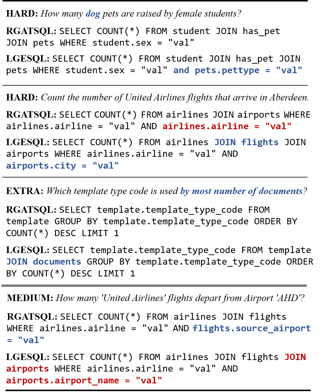
Figure 7: Case study: the first three cases are positive samples while the last one is negative. The input question is represented by its level of difficulty. FROM conditions are omitted here for brevity and cell values in the SQL queries are replaced with placeholders “val”.

In Figure 7, we compare the SQL queries generated by our LGESQL model with those created by the baseline model RGATSQL. We notice that LGESQL performs better than the baseline system, especially on examples that involve the JOIN operation of multiple tables. For instance, in the second case where the connection of three tables are included, RGATSQL fails to identify the existence of table flights. Thus, it is unable to predict the WHERE condition about the destination city and does repeat work. In the third case, our LGESQL still successfully constructs a connected schema sub-graph by linking table “template” to “documents”. Sadly, the RGATSQL model neglects the occurrence of “documents” again. However, in the last case, our LGESQL is stupid to introduce an unnecessary table “airports”. It ignores the situation that table “flights” has one column “source_airport” which already satisfies the requirement.

5 Related Work

Encoding Problem for Text-to-SQL

To tackle the joint encoding problem of the question and database schema, Xu et al. (2017) proposes “column attention” strategy to gather information from columns for each question word. TypeSQL Yu et al. (2018a) incorporates prior knowledge of column types and schema linking as additional input features. Bogin et al. (2019a) and Chen et al. (2021) deal with the graph structure of database schema via GNN. EditSQL Zhang et al. (2019b) considers “co-attention” between question words and database schema nodes similar to the common practice in text matching Chen et al. (2017). BRIDGE Lin et al. (2020) further leverages the database content to augment the column representation. The most advanced method RATSQL Wang et al. (2020a), utilizes a complete relational graph attention neural network to handle various pre-defined relations. In this work, we further consider both local and non-local, dynamic and static edge features among different types of nodes with a line graph.

Heterogeneous Graph Neural Network

Apart from the structural topology, a heterogeneous graph Shi et al. (2016) also contains multiple types of nodes and edges. To address the heterogeneity of node attributes, Zhang et al. (2019a) designs a type-based content encoder and Fu et al. (2020) utilizes a type-specific linear transformation. For edges, relational graph convolution network (RGCN, Schlichtkrull et al., 2018) and relational graph attention network (RGAT, Wang et al., 2020b) have been proposed to parameterize different relations. HAN Wang et al. (2019b) converts the original heterogeneous graph into multiple homogeneous graphs and applies a hierarchical attention mechanism to the meta-path-based sub-graphs. Similar ideas have been adopted in dialogue state tracking Chen et al. (2020b, 2019a), dialogue policy learning Chen et al. (2018) and text matching Chen et al. (2020c); Lyu et al. (2021) to handle heterogeneous inputs. In another branch, Chen et al. (2019b), Zhu et al. (2019) and Zhao et al. (2020) construct the line graph of the original graph and explicitly model the computation over edge features. In this work, we borrow the idea of a line graph and update both node and edge features via iteration over dual graphs.

6 Conclusion

In this work, we utilize the line graph to update the edge features in the heterogeneous graph for the text-to-SQL task. Through the iteration over the structural connections in the line graph, local edges can incorporate multi-hop relational features and capture significant meta-paths. By further integrating non-local relations, the encoder can learn from multiple views and attend to remote nodes with shortcuts. In the future, we will investigate more useful meta-paths and explore more effective methods to deal with different meta-path-based neighbors.

Appendix A Local and Non-Local Relations

Source $x$	Target $y$	Relation	Description
Q	Q	Distance+1	$y$ is the next word of $x$.
C	C	ForeignKey	$y$ is the foreign key of $x$.
T	C	Has	The column $y$ belongs to the table $x$.
		PrimaryKey	The column $y$ is the primary key of the table $x$.
Q	T	NoMatch	No overlapping between $x$ and $y$.
		PartialMatch	$x$ is part of $y$, but the entire question does not contain $y$.
		ExactMatch	$x$ is part of $y$, and $y$ is a span of the entire question.
Q	C	NoMatch	No overlapping between $x$ and $y$.
		PartialMatch	$x$ is part of $y$, but the entire question does not contain $y$.
		ExactMatch	$x$ is part of $y$, and $y$ is a span of the entire question.
		ValueMatch	$x$ is part of the candidate cell values of column $y$.

Table 6: The checklist of all local relations used in our experiments. All relations above are asymmetric. For brevity, we only show one direction, and the opposite can be easily inferred. Q/T/C stands for Question/Table/Column node respectively.

In this work, meta-paths with length $1$ are local relations, and other meta-paths are non-local relations. Specifically, Table 6 provides the list of all local relations according to the types of source and target nodes. Notice that we preserve the NoMatch relation because there is no overlapping between the entire question and any schema item in some cases. This relaxation will dramatically increase the number of edges in the line graph. To resolve it, we remove edges in the line graph that the source and target nodes both represent relation types of Match series. In other words, we prevent information propagating between these bipartite connections during the iteration of the line graph.

The checklist in Table 6 is only a subset of all relations defined in RATSQL Wang et al. (2020a). For the remaining relations, we treat them as non-local relations for a fair comparison to the baseline system RATSQL.

Appendix B Details of Text-to-SQL Decoder

B.1 ASDL Grammar

Figure 8: The ASDL grammar for SQL in our implementation.

The complete grammar used to translate the SQL into a series of actions is provided in Figure 8. Here are some criteria when we design the abstract syntax description language (ASDL, Wang et al., 1997) for the target SQL queries:

1. Keep the length of the action sequence short to prevent the long-term forgetting problem in the auto-regressive decoder. To achieve this goal, we remove the optional operator “?” defined in Wang et al. (1997) and extend the number of constructors by enumeration. For example, we expand all solutions of type sql_unit according to the existence of different clauses.

2. Hierarchically, group and re-use the same type in a top-down manner for parameter sharing. For example, we use the same type col_unit when choosing columns in different clauses and create the type val_unit such that both the SELECT clause and CONDITION clauses can refer to it.

3. When generating a list of items of the same type, instead of emitting a special action Reduce as the symbol of termination Yin and Neubig (2017), we enumerate all possible number of occurrences in the training set (see the constructors for type select and from in Figure 8). Then, we generate each item based on this quantitative limitation. Preliminary experimental results prove that thinking in advance is better than a lazy decision.

Our grammar can cover $98.7\%$ and $98.2\%$ cases in the training and validation dataset, respectively.

B.2 Decoder Architecture

Given the encoded memory $\mathbf{X}=[\mathbf{X}_{q};\mathbf{X}_{t};\mathbf{X}_{c}]\in\mathbb{R}^{|V^{n}|\times d}$, where $|V^{n}|=|Q|+|T|+|C|$, the goal of a text-to-SQL decoder is to produce a sequence of actions which can construct the corresponding AST of the target SQL query. In our experiments, we utilize a single layer ordered neurons LSTM (ON-LSTM, Shen et al., 2019) as the auto-regressive decoder. Firstly, we initialize the decoder state $\mathbf{h}_{0}$ via attentive pooling over the memory $\mathbf{X}$.

$$a_{i}= \text{softmax}_{i}\ \text{tanh}(\mathbf{x}_{i}\mathbf{W}_{0})\mathbf{v}_{0}^{\mathrm{T}},$$

$$\tilde{\mathbf{h}}_{0}= \sum_{i}a_{i}\mathbf{x}_{i},$$

$$\mathbf{h}_{0}= \text{tanh}(\tilde{\mathbf{h}}_{0}\mathbf{W}_{1}),$$

where $\mathbf{v}_{0}$ is a trainable row vector and $\mathbf{W}_{0},\mathbf{W}_{1}$ are parameter matrices. Then, in the structured ON-LSTM decoder, the hidden states at each timestep $j$ is updated as

$$\mathbf{m}_{j},\mathbf{h}_{j}=\text{ON-LSTM}([\mathbf{a}_{j-1};\mathbf{a}_{p_{j}}; \mathbf{h}_{p_{j}};\mathbf{n}_{j}],$$

$$\mathbf{m}_{j-1},\mathbf{h}_{j-1}),$$

where $\mathbf{m}_{j}$ is the cell state of the $j$-th timestep, $\mathbf{a}_{j-1}$ is the embedding of the previous action, $\mathbf{a}_{p_{j}}$ is the embedding of parent action, $\mathbf{h}_{p_{t}}$ is the embedding of parent hidden state, and $\mathbf{n}_{j}$ denotes the type embedding of the current frontier node . Given the current decoder state $\mathbf{h}_{j}$, we adopt multi-head attention ($8$ heads) mechanism to calculate the context vector $\tilde{\mathbf{h}}_{j}$ over $\mathbf{X}$. This context vector is concatenated with $\mathbf{h}_{j}$ and passed into a 2-layer MLP with tanh activation unit to obtain the attention vector $\mathbf{h}_{j}^{att}$. The dimension of $\mathbf{h}_{j}^{att}$ is $512$.

For ApplyRule action, the probability distribution is computed by a softmax classification layer:

$$P(a_{j}=\textsc{ApplyRule}[R]|a_{<j},\mathbf{X})=\\ \text{softmax}_{R}(\mathbf{h}^{att}_{j}\mathbf{W}_{\text{R}}).$$

For SelectTable action, we directly copy the table $t_{i}$ from the encoded memory $\mathbf{X}_{t}$.

$$\zeta_{ji}^{h}= \text{softmax}_{i}(\mathbf{h}^{att}_{j}\mathbf{W}^{h}_{tq})(\mathbf{x}_{t_{i}}\mathbf{W}^{h}_{tk})^{\mathrm{T}},$$

$$P(a_{j}= \textsc{SelectTable}[t_{i}]|a_{<j},\mathbf{X})=\frac{1}{H}\sum_{h=1}^{H}\zeta^{h}_{ji}.$$

To be consistent, we also apply the multi-head attention mechanism here with $H=8$ heads. The calculation of SelectColumn action is similar with different network parameters.

Appendix C Graph Pruning

Similar ideas have been proposed by Bogin et al. (2019b) and Yu et al. (2020). Our proposed task differs from their methods in two aspects:

Prediction target

Yu et al. (2020) devises several syntactic roles for schema items and performs multi-class classification instead of binary discrimination. Based on our assumption, the encoder is responsible for the discrimination capability while the decoder organizes different schema items and components into a complete semantic frame. Thus, we simplify the training target into binary labels.

Combination method

Bogin et al. (2019b) utilizes another RGCN to calculate the relevance score for each schema item in Global-GNNSQL. This score is incorporated into the encoder RGCN as a soft input coefficient. Different from this cascaded method, graph pruning is employed in a multitasking manner. We have tried different approaches to combine this auxiliary module with the primary text-to-SQL model in our preliminary experiments, such as:

1) Similar to Bogin et al. (2019b), we utilize a separate graph encoder to conduct graph pruning firstly, and use another refined graph encoder (the same architecture, e.g., RGAT) to jointly encode the pruned schema graph and the question. These two encoders can share network parameters of only the embeddings or more upper GNN layers. If they share all $8$ layers, the entire encoder will degenerate from the pipelined mode into our multitasking fashion. Empirical results in Table 7 demonstrate that when these two encoders share more layers, the performance of the text-to-SQL model is better.

mode	# layers shared	dev acc
pipeline	0	60.74
$\Downarrow$	4	61.63
multitasking	8	62.53

Table 7: Variation of performances when gradually increasing the number of layers shared between the pruning and the main encoders.

2) We can constrain the text-to-SQL decoder to only attend and retrieve schema items from the pruned encoded memory when calculating attention vectors and select columns or tables. In other words, the graph pruning module and the text-to-SQL decoder are connected in a cascaded way. Through pilot experiments, we observe the flagrant training-inference inconsistency problem. The text-to-SQL decoder is trained upon the golden schema items, but it depends on the predicted options from the graph pruning module during evaluation. Even if we endeavor various sampling-based methods (such as random sampling, sampling from current module predictions, or sampling from neighboring nodes of the golden schema graph) to inject some noise during training, the performance is merely competitive to that with multitasking. Therefore, based on Occam’s Razor Theorem, we only treat graph pruning as an auxiliary output module.

References

- Androutsopoulos et al. (1995) Ion Androutsopoulos, Graeme D Ritchie, and Peter Thanisch. 1995. Natural language interfaces to databases-an introduction. arXiv preprint cmp-lg/9503016.
- Bahdanau et al. (2015) Dzmitry Bahdanau, Kyunghyun Cho, and Yoshua Bengio. 2015. Neural machine translation by jointly learning to align and translate. In 3rd International Conference on Learning Representations, ICLR 2015, San Diego, CA, USA, May 7-9, 2015, Conference Track Proceedings.
- Bogin et al. (2019a) Ben Bogin, Jonathan Berant, and Matt Gardner. 2019a. Representing schema structure with graph neural networks for text-to-SQL parsing. In Proceedings of the 57th Annual Meeting of the Association for Computational Linguistics, pages 4560–4565, Florence, Italy. Association for Computational Linguistics.
- Bogin et al. (2019b) Ben Bogin, Matt Gardner, and Jonathan Berant. 2019b. Global reasoning over database structures for text-to-SQL parsing. In Proceedings of the 2019 Conference on Empirical Methods in Natural Language Processing and the 9th International Joint Conference on Natural Language Processing (EMNLP-IJCNLP), pages 3659–3664, Hong Kong, China. Association for Computational Linguistics.
- Chen et al. (2020a) Deli Chen, Yankai Lin, Wei Li, Peng Li, Jie Zhou, and Xu Sun. 2020a. Measuring and relieving the over-smoothing problem for graph neural networks from the topological view. In Proceedings of the AAAI Conference on Artificial Intelligence, volume 34, pages 3438–3445.
- Chen et al. (2019a) Lu Chen, Zhi Chen, Bowen Tan, Sishan Long, Milica Gasic, and Kai Yu. 2019a. Agentgraph: Towards universal dialogue management with structured deep reinforcement learning. CoRR, abs/1905.11259.
- Chen et al. (2020b) Lu Chen, Boer Lv, Chi Wang, Su Zhu, Bowen Tan, and Kai Yu. 2020b. Schema-guided multi-domain dialogue state tracking with graph attention neural networks. In Proceedings of the AAAI Conference on Artificial Intelligence, volume 34, pages 7521–7528.
- Chen et al. (2018) Lu Chen, Bowen Tan, Sishan Long, and Kai Yu. 2018. Structured dialogue policy with graph neural networks. In Proceedings of the 27th International Conference on Computational Linguistics (COLING), pages 1257––1268.
- Chen et al. (2020c) Lu Chen, Yanbin Zhao, Boer Lyu, Lesheng Jin, Zhi Chen, Su Zhu, and Kai Yu. 2020c. Neural graph matching networks for Chinese short text matching. In Proceedings of the 58th Annual Meeting of the Association for Computational Linguistics, pages 6152–6158, Online. Association for Computational Linguistics.
- Chen et al. (2017) Qian Chen, Xiaodan Zhu, Zhen-Hua Ling, Si Wei, Hui Jiang, and Diana Inkpen. 2017. Enhanced LSTM for natural language inference. In Proceedings of the 55th Annual Meeting of the Association for Computational Linguistics (Volume 1: Long Papers), pages 1657–1668, Vancouver, Canada. Association for Computational Linguistics.
- Chen et al. (2019b) Zhengdao Chen, Lisha Li, and Joan Bruna. 2019b. Supervised community detection with line graph neural networks. In 7th International Conference on Learning Representations, ICLR 2019, New Orleans, LA, USA, May 6-9, 2019. OpenReview.net.
- Chen et al. (2021) Zhi Chen, Lu Chen, Yanbin Zhao, Ruisheng Cao, Zihan Xu, Su Zhu, and Kai Yu. 2021. ShadowGNN: Graph projection neural network for text-to-SQL parser. In Proceedings of the 2021 Conference of the North American Chapter of the Association for Computational Linguistics: Human Language Technologies, pages 5567–5577, Online. Association for Computational Linguistics.
- Clark et al. (2020) Kevin Clark, Minh-Thang Luong, Quoc V. Le, and Christopher D. Manning. 2020. ELECTRA: pre-training text encoders as discriminators rather than generators. In 8th International Conference on Learning Representations, ICLR 2020, Addis Ababa, Ethiopia, April 26-30, 2020. OpenReview.net.
- Deng et al. (2021) Xiang Deng, Ahmed Hassan Awadallah, Christopher Meek, Oleksandr Polozov, Huan Sun, and Matthew Richardson. 2021. Structure-grounded pretraining for text-to-SQL. In Proceedings of the 2021 Conference of the North American Chapter of the Association for Computational Linguistics: Human Language Technologies, pages 1337–1350, Online. Association for Computational Linguistics.
- Devlin et al. (2019) Jacob Devlin, Ming-Wei Chang, Kenton Lee, and Kristina Toutanova. 2019. BERT: Pre-training of deep bidirectional transformers for language understanding. In Proceedings of the 2019 Conference of the North American Chapter of the Association for Computational Linguistics: Human Language Technologies, Volume 1 (Long and Short Papers), pages 4171–4186, Minneapolis, Minnesota. Association for Computational Linguistics.
- Dozat and Manning (2017) Timothy Dozat and Christopher D. Manning. 2017. Deep biaffine attention for neural dependency parsing. In 5th International Conference on Learning Representations, ICLR 2017, Toulon, France, April 24-26, 2017, Conference Track Proceedings. OpenReview.net.
- Fu et al. (2020) Xinyu Fu, Jiani Zhang, Ziqiao Meng, and Irwin King. 2020. Magnn: metapath aggregated graph neural network for heterogeneous graph embedding. In Proceedings of The Web Conference 2020, pages 2331–2341.
- Gal and Ghahramani (2016) Yarin Gal and Zoubin Ghahramani. 2016. A theoretically grounded application of dropout in recurrent neural networks. In Advances in Neural Information Processing Systems 29: Annual Conference on Neural Information Processing Systems 2016, December 5-10, 2016, Barcelona, Spain, pages 1019–1027.
- Gross and Yellen (2005) Jonathan L Gross and Jay Yellen. 2005. Graph theory and its applications. CRC press.
- Guo et al. (2019) Jiaqi Guo, Zecheng Zhan, Yan Gao, Yan Xiao, Jian-Guang Lou, Ting Liu, and Dongmei Zhang. 2019. Towards complex text-to-SQL in cross-domain database with intermediate representation. In Proceedings of the 57th Annual Meeting of the Association for Computational Linguistics, pages 4524–4535, Florence, Italy. Association for Computational Linguistics.
- Hochreiter and Schmidhuber (1997) Sepp Hochreiter and Jürgen Schmidhuber. 1997. Long short-term memory. Neural computation, 9(8):1735–1780.
- Iyer et al. (2017) Srinivasan Iyer, Ioannis Konstas, Alvin Cheung, Jayant Krishnamurthy, and Luke Zettlemoyer. 2017. Learning a neural semantic parser from user feedback. In Proceedings of the 55th Annual Meeting of the Association for Computational Linguistics (Volume 1: Long Papers), pages 963–973, Vancouver, Canada. Association for Computational Linguistics.
- Kong et al. (2012) Xiangnan Kong, Philip S Yu, Ying Ding, and David J Wild. 2012. Meta path-based collective classification in heterogeneous information networks. In Proceedings of the 21st ACM international conference on Information and knowledge management, pages 1567–1571.
- Lao and Cohen (2010) Ni Lao and William W Cohen. 2010. Relational retrieval using a combination of path-constrained random walks. Machine learning, 81(1):53–67.
- Li and Jagadish (2014) Fei Li and HV Jagadish. 2014. Constructing an interactive natural language interface for relational databases. Proceedings of the VLDB Endowment, 8:73–84.
- Lin et al. (2020) Xi Victoria Lin, Richard Socher, and Caiming Xiong. 2020. Bridging textual and tabular data for cross-domain text-to-SQL semantic parsing. In Findings of the Association for Computational Linguistics: EMNLP 2020, pages 4870–4888, Online. Association for Computational Linguistics.
- Loshchilov and Hutter (2019) Ilya Loshchilov and Frank Hutter. 2019. Decoupled weight decay regularization. In 7th International Conference on Learning Representations, ICLR 2019, New Orleans, LA, USA, May 6-9, 2019. OpenReview.net.
- Lyu et al. (2021) Boer Lyu, Lu Chen, Su Zhu, and Kai Yu. 2021. Let: Linguistic knowledge enhanced graph transformer for chinese short text matching.
- Paszke et al. (2019) Adam Paszke, Sam Gross, Francisco Massa, Adam Lerer, James Bradbury, Gregory Chanan, Trevor Killeen, Zeming Lin, Natalia Gimelshein, Luca Antiga, Alban Desmaison, Andreas Köpf, Edward Yang, Zachary DeVito, Martin Raison, Alykhan Tejani, Sasank Chilamkurthy, Benoit Steiner, Lu Fang, Junjie Bai, and Soumith Chintala. 2019. Pytorch: An imperative style, high-performance deep learning library. In Advances in Neural Information Processing Systems 32: Annual Conference on Neural Information Processing Systems 2019, NeurIPS 2019, December 8-14, 2019, Vancouver, BC, Canada, pages 8024–8035.
- Pennington et al. (2014) Jeffrey Pennington, Richard Socher, and Christopher Manning. 2014. GloVe: Global vectors for word representation. In Proceedings of the 2014 Conference on Empirical Methods in Natural Language Processing (EMNLP), pages 1532–1543, Doha, Qatar. Association for Computational Linguistics.
- Popescu et al. (2003) Ana-Maria Popescu, Oren Etzioni, and Henry Kautz. 2003. Towards a theory of natural language interfaces to databases. In Proceedings of the 8th international conference on Intelligent user interfaces, pages 149–157.
- Qi et al. (2020) Peng Qi, Yuhao Zhang, Yuhui Zhang, Jason Bolton, and Christopher D. Manning. 2020. Stanza: A python natural language processing toolkit for many human languages. In Proceedings of the 58th Annual Meeting of the Association for Computational Linguistics: System Demonstrations, pages 101–108, Online. Association for Computational Linguistics.
- Rubin and Berant (2021) Ohad Rubin and Jonathan Berant. 2021. SmBoP: Semi-autoregressive bottom-up semantic parsing. In Proceedings of the 2021 Conference of the North American Chapter of the Association for Computational Linguistics: Human Language Technologies, pages 311–324, Online. Association for Computational Linguistics.
- Scarselli et al. (2008) Franco Scarselli, Marco Gori, Ah Chung Tsoi, Markus Hagenbuchner, and Gabriele Monfardini. 2008. The graph neural network model. IEEE transactions on neural networks, 20(1):61–80.
- Schlichtkrull et al. (2018) Michael Schlichtkrull, Thomas N Kipf, Peter Bloem, Rianne Van Den Berg, Ivan Titov, and Max Welling. 2018. Modeling relational data with graph convolutional networks. In European semantic web conference, pages 593–607. Springer.
- Shaw et al. (2018) Peter Shaw, Jakob Uszkoreit, and Ashish Vaswani. 2018. Self-attention with relative position representations. In Proceedings of the 2018 Conference of the North American Chapter of the Association for Computational Linguistics: Human Language Technologies, Volume 2 (Short Papers), pages 464–468, New Orleans, Louisiana. Association for Computational Linguistics.
- Shen et al. (2019) Yikang Shen, Shawn Tan, Alessandro Sordoni, and Aaron C. Courville. 2019. Ordered neurons: Integrating tree structures into recurrent neural networks. In 7th International Conference on Learning Representations, ICLR 2019, New Orleans, LA, USA, May 6-9, 2019. OpenReview.net.
- Shi et al. (2016) Chuan Shi, Yitong Li, Jiawei Zhang, Yizhou Sun, and S Yu Philip. 2016. A survey of heterogeneous information network analysis. IEEE Transactions on Knowledge and Data Engineering, 29(1):17–37.
- Shi et al. (2020) Peng Shi, Patrick Ng, Zhiguo Wang, Henghui Zhu, Alexander Hanbo Li, Jun Wang, Cícero Nogueira dos Santos, and Bing Xiang. 2020. Learning contextual representations for semantic parsing with generation-augmented pre-training. CoRR, abs/2012.10309.
- Suhr et al. (2020) Alane Suhr, Ming-Wei Chang, Peter Shaw, and Kenton Lee. 2020. Exploring unexplored generalization challenges for cross-database semantic parsing. In Proceedings of the 58th Annual Meeting of the Association for Computational Linguistics, pages 8372–8388, Online. Association for Computational Linguistics.
- Sutskever et al. (2014) Ilya Sutskever, Oriol Vinyals, and Quoc V. Le. 2014. Sequence to sequence learning with neural networks. In Advances in Neural Information Processing Systems 27: Annual Conference on Neural Information Processing Systems 2014, December 8-13 2014, Montreal, Quebec, Canada, pages 3104–3112.
- Vaswani et al. (2017) Ashish Vaswani, Noam Shazeer, Niki Parmar, Jakob Uszkoreit, Llion Jones, Aidan N Gomez, Lukasz Kaiser, and Illia Polosukhin. 2017. Attention is all you need. arXiv preprint arXiv:1706.03762.
- Wang et al. (2020a) Bailin Wang, Richard Shin, Xiaodong Liu, Oleksandr Polozov, and Matthew Richardson. 2020a. RAT-SQL: Relation-aware schema encoding and linking for text-to-SQL parsers. In Proceedings of the 58th Annual Meeting of the Association for Computational Linguistics, pages 7567–7578, Online. Association for Computational Linguistics.
- Wang et al. (1997) Daniel C Wang, Andrew W Appel, Jeffrey L Korn, and Christopher S Serra. 1997. The zephyr abstract syntax description language. In DSL, volume 97, pages 17–17.
- Wang et al. (2020b) Kai Wang, Weizhou Shen, Yunyi Yang, Xiaojun Quan, and Rui Wang. 2020b. Relational graph attention network for aspect-based sentiment analysis. In Proceedings of the 58th Annual Meeting of the Association for Computational Linguistics, pages 3229–3238, Online. Association for Computational Linguistics.
- Wang et al. (2019a) Minjie Wang, Da Zheng, Zihao Ye, Quan Gan, Mufei Li, Xiang Song, Jinjing Zhou, Chao Ma, Lingfan Yu, Yu Gai, Tianjun Xiao, Tong He, George Karypis, Jinyang Li, and Zheng Zhang. 2019a. Deep graph library: A graph-centric, highly-performant package for graph neural networks. arXiv preprint arXiv:1909.01315.
- Wang et al. (2019b) Xiao Wang, Houye Ji, Chuan Shi, Bai Wang, Yanfang Ye, Peng Cui, and Philip S Yu. 2019b. Heterogeneous graph attention network. In The World Wide Web Conference, pages 2022–2032.
- Xu et al. (2021) Peng Xu, Dhruv Kumar, Wei Yang, Wenjie Zi, Keyi Tang, Chenyang Huang, Jackie Chi Kit Cheung, Simon J. D. Prince, and Yanshuai Cao. 2021. Optimizing deeper transformers on small datasets.
- Xu et al. (2017) Xiaojun Xu, Chang Liu, and Dawn Song. 2017. Sqlnet: Generating structured queries from natural language without reinforcement learning. arXiv preprint arXiv:1711.04436.
- Yaghmazadeh et al. (2017) Navid Yaghmazadeh, Yuepeng Wang, Isil Dillig, and Thomas Dillig. 2017. Sqlizer: query synthesis from natural language. Proceedings of the ACM on Programming Languages, 1:1–26.
- Yin and Neubig (2017) Pengcheng Yin and Graham Neubig. 2017. A syntactic neural model for general-purpose code generation. In Proceedings of the 55th Annual Meeting of the Association for Computational Linguistics (Volume 1: Long Papers), pages 440–450, Vancouver, Canada. Association for Computational Linguistics.
- Yu et al. (2018a) Tao Yu, Zifan Li, Zilin Zhang, Rui Zhang, and Dragomir Radev. 2018a. TypeSQL: Knowledge-based type-aware neural text-to-SQL generation. In Proceedings of the 2018 Conference of the North American Chapter of the Association for Computational Linguistics: Human Language Technologies, Volume 2 (Short Papers), pages 588–594, New Orleans, Louisiana. Association for Computational Linguistics.
- Yu et al. (2020) Tao Yu, Chien-Sheng Wu, Xi Victoria Lin, Bailin Wang, Yi Chern Tan, Xinyi Yang, Dragomir R. Radev, Richard Socher, and Caiming Xiong. 2020. Grappa: Grammar-augmented pre-training for table semantic parsing. CoRR, abs/2009.13845.
- Yu et al. (2018b) Tao Yu, Rui Zhang, Kai Yang, Michihiro Yasunaga, Dongxu Wang, Zifan Li, James Ma, Irene Li, Qingning Yao, Shanelle Roman, Zilin Zhang, and Dragomir Radev. 2018b. Spider: A large-scale human-labeled dataset for complex and cross-domain semantic parsing and text-to-SQL task. In Proceedings of the 2018 Conference on Empirical Methods in Natural Language Processing, pages 3911–3921, Brussels, Belgium. Association for Computational Linguistics.
- Zelle and Mooney (1996) John M Zelle and Raymond J Mooney. 1996. Learning to parse database queries using inductive logic programming. In Proceedings of the national conference on artificial intelligence, pages 1050–1055.
- Zhang et al. (2019a) Chuxu Zhang, Dongjin Song, Chao Huang, Ananthram Swami, and Nitesh V Chawla. 2019a. Heterogeneous graph neural network. In Proceedings of the 25th ACM SIGKDD International Conference on Knowledge Discovery & Data Mining, pages 793–803.
- Zhang et al. (2019b) Rui Zhang, Tao Yu, Heyang Er, Sungrok Shim, Eric Xue, Xi Victoria Lin, Tianze Shi, Caiming Xiong, Richard Socher, and Dragomir Radev. 2019b. Editing-based SQL query generation for cross-domain context-dependent questions. In Proceedings of the 2019 Conference on Empirical Methods in Natural Language Processing and the 9th International Joint Conference on Natural Language Processing (EMNLP-IJCNLP), pages 5338–5349, Hong Kong, China. Association for Computational Linguistics.
- Zhao et al. (2020) Yanbin Zhao, Lu Chen, Zhi Chen, Ruisheng Cao, Su Zhu, and Kai Yu. 2020. Line graph enhanced AMR-to-text generation with mix-order graph attention networks. In Proceedings of the 58th Annual Meeting of the Association for Computational Linguistics, pages 732–741, Online. Association for Computational Linguistics.
- Zhong et al. (2020) Victor Zhong, Mike Lewis, Sida I. Wang, and Luke Zettlemoyer. 2020. Grounded adaptation for zero-shot executable semantic parsing. In Proceedings of the 2020 Conference on Empirical Methods in Natural Language Processing (EMNLP), pages 6869–6882, Online. Association for Computational Linguistics.
- Zhong et al. (2017) Victor Zhong, Caiming Xiong, and Richard Socher. 2017. Seq2sql: Generating structured queries from natural language using reinforcement learning. arXiv preprint arXiv:1709.00103.
- Zhu et al. (2019) Shichao Zhu, Chuan Zhou, Shirui Pan, Xingquan Zhu, and Bin Wang. 2019. Relation structure-aware heterogeneous graph neural network. In 2019 IEEE International Conference on Data Mining (ICDM), pages 1534–1539.