Is Sparse Attention more Interpretable?

Abstract

Sparse attention has been claimed to increase model interpretability under the assumption that it highlights influential inputs. Yet the attention distribution is typically over representations internal to the model rather than the inputs themselves, suggesting this assumption may not have merit. We build on the recent work exploring the interpretability of attention; we design a set of experiments to help us understand how sparsity affects our ability to use attention as an explainability tool. On three text classification tasks, we verify that only a weak relationship between inputs and co-indexed intermediate representations exists—under sparse attention and otherwise. Further, we do not find any plausible mappings from sparse attention distributions to a sparse set of influential inputs through other avenues. Rather, we observe in this setting that inducing sparsity may make it less plausible that attention can be used as a tool for understanding model behavior.

1 Introduction

Interpretability research in natural language processing (NLP) is becoming increasingly important as complex models are applied to more and more downstream decision making tasks. In light of this, many researchers have turned to the attention mechanism, which has not only led to impressive performance improvements in neural models, but has also been claimed to offer insights into how models make decisions. Specifically, a number of works imply or directly state that one may inspect the attention distribution to determine the amount of influence each input token has in a model’s decision-making process (Xie et al., 2017; Mullenbach et al., 2018; Niculae et al., 2018, inter alia).

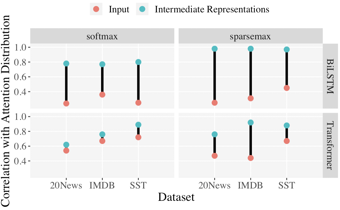
Figure 1: Correlation between the attention distribution and gradient-based FI measures. We see a notably stronger correlation between attention and FI of intermediate representation than of inputs across all models.

Many lines of work have gone on to exploit this assumption when building their own “interpretable” models or analysis tools Yang et al. (2016); Tu et al. (2016); De-Arteaga et al. (2019); one subset has even tried to make models with attention more interpretable by inducing sparsity—a common attribute of interpretable models Lipton (2018); Rudin (2019)—in attention weights, with the motivation that this allows model decisions to be mapped to a limited number of items Martins and Astudillo (2016); Malaviya et al. (2018); Zhang et al. (2019). Yet, there lacks concrete reasoning or evidence that sparse attention weights leads to more interpretable models: customarily, attention is not directly over the model’s inputs, but rather over some representation internal to the model, e.g. the hidden states of a recurrent network or contextual embeddings of a Transformer (see Fig. 1). Importantly, these internal representations do not solely encode information from the input token they are co-indexed with Salehinejad et al. (2017); Brunner et al. (2020), but rather from a range of inputs. This presents the question: if internal representations themselves may not be interpretable, can we actually deduce anything from “interpretable” attention weights?

We build on the recent line of work challenging the validity of attention-as-explanation methods (Jain and Wallace, 2019; Serrano and Smith, 2019; Grimsley et al., 2020, inter alia) and specifically examine how sparsity affects their observations. To this end, we introduce a novel entropy-based metric to measure the dispersion of inputs’ influence, rather than just their magnitudes. Through experiments on three text classification tasks, utilizing both LSTM and Transformer-based models, we observe how sparse attention affects the results of Jain and Wallace (2019) and Wiegreffe and Pinter (2019), additionally exploring whether it allows us to identify a core set of inputs that are important to models’ decisions. We find we are unable to identify such a set when using sparse attention; rather, it appears that encouraging sparsity may simultaneously encourage a higher degree of contextualization in intermediate representations. We further observe a decrease in the correlation between the attention distribution and input feature importance measures, which exacerbates issues found by prior works. The primary conclusion of our work is that we should not believe sparse attention enhances model interpretability until we have concrete reasons to believe so; in this preliminary analysis, we do not find any such evidence.

2 Attention-based Neural Networks

We consider inputs $\mathbf{x}=x_{1}\cdots x_{n}\in\mathcal{V}^{n}$ of length $n$ where the tokens from taken from an alphabet $\mathcal{V}$. We denote the embedding of $\mathbf{x}$, e.g., its one hot encoding or (more commonly) a linear transformation of its one-hot encoding with an embedding matrix $E\in\mathbb{R}^{d\times|\mathcal{V}|}$, as $X^{(e)}\in\mathbb{R}^{d\times n}$. Our embedded input $X^{(e)}$ is then fed to an encoder, which produces $n$ intermediate representations $I=[\mathbf{h}_{1};\dots;\mathbf{h}_{n}]\in\mathbb{R}^{m\times n}$, where $\mathbf{h}_{i}\in\mathbb{R}^{m}$ and $m$ is a hyperparameter of the encoder. This transformation is quite architecture dependent.

An alignment function $A(\cdot,\cdot)$ maps a query $\mathbf{q}$ and a key $K$ to weights $\mathbf{a}^{(t)}$ for a decoding time step $t$; we subsequently drop $t$ for simplicity.author=ryan,color=violet!40,size=,fancyline,caption=,]I added this because $t$ magically disappeared. Is that okay? In colloquial terms, $A$ chooses which values of $K$ should receive the most attention based on $\mathbf{q}$, which is then represented in the vector $\mathbf{a}^{(t)}\in\mathbb{R}^{n}$. For the NLP tasks we consider, we have $K=I=[\mathbf{h}_{1};\dots;\mathbf{h}_{n}]$, the encoder outputs. A query $\mathbf{q}$ may be, e.g., a representation of the question in question answering.

The weights $\mathbf{a}$ are projected to sum to 1, which results in the attention distribution ${\boldsymbol{\alpha}}$. Mathematically, this is done via a projection onto the probability simplex using a projection function $\phi$, e.g., softmax or sparsemax. We then compute the context vector as $\mathbf{c}=\sum_{i=1}^{n}\alpha_{i}\,\mathbf{h}_{i}$. This context vector is fed to a decoder, whose structure is again architecture dependent, which generates a (possibly unnormalized) probability distribution over the set of labels ${\cal Y}$, where ${\cal Y}$ is defined by the task.

Attention.

We experiment with two methods of constructing an attention distribution: (1) additive attention, proposed by Bahdanau et al. (2015): $A(K,\mathbf{q})_{i}=\mathbf{v}^{\top}\tanh(W_{1}K_{i}+W_{2}\mathbf{q})$ and (2) the scaled dot product alignment function, as in the Transformer network: $A(K,\mathbf{q})=\frac{K^{\top}\mathbf{q}}{\sqrt{m}}$ where $\mathbf{v}\in\mathbb{R}^{l}$ and $W_{1},W_{2}\in\mathbb{R}^{l\times m}$ are weight matrices. Note that the original (without attention) neural encoder–decoder architecture, as in Sutskever et al. (2014), can be recovered with alignment function $A(\cdot,\cdot)=[0,\dots,0,1]$, i.e., only the last of the $n$ intermediate representations is given to the decoder.

Projection Functions.

A projection function $\phi$ takes the output of the alignment function and maps it to a valid probability distribution: $\phi:\mathbb{R}^{n}\rightarrow\Delta^{n-1}$. The standard projection function is softmax:

$$\phi_{\mathrm{soft}}(\mathbf{z}) =\frac{\exp(\mathbf{z})}{\sum_{i\in[n]}\exp(z_{i})}$$ (1)

$$=\operatorname*{argmin}_{\mathbf{p}\in\Delta^{n-1}}\left(\sum_{i\in[n]}p_{i}\log p_{i}-\mathbf{p}^{\top}\mathbf{z}\right)$$

However, softmax leads to non-sparse solutions as an entry $\phi_{\mathrm{soft}}(\mathbf{z})_{i}$ can only be $0$ if $x_{i}\!=\!-\infty$. Alternatively, Martins and Astudillo (2016) introduce sparsemax, which can output sparse distributions:

$$\phi_{\mathrm{sparse}}(\mathbf{z})=\operatorname*{argmin}_{\mathbf{p}\in\Delta^{n-1}}\left\lVert\mathbf{p}-\mathbf{z}\right\rVert^{2}_{2}$$ (2)

In words, sparsemax directly maps $\mathbf{z}$ onto the probability simplex, which often leads to solutions on the boundary, i.e. where at least one entry of $\mathbf{p}$ is $0$. The formulation of sparsemax in Eq. 2 does not give us an explicit medium for controlling the degree of sparsity. The $\alpha$-entmax Peters et al. (2019) and sparsegen Laha et al. (2018) transformations fill this gap; we employ the latter:

$$\phi_{\mathrm{sparseg}}(\mathbf{z})=\operatorname*{argmin}_{\mathbf{p}\in\Delta^{n-1}}\left\lVert\mathbf{p}-g(\mathbf{z})\right\rVert^{2}_{2}-\lambda\left\lVert\mathbf{p}\right\rVert^{2}_{2}$$ (3)

where the degree of sparsity can be tuned via the hyperparameter $\lambda\in(-\infty,1)$. Note that a larger $\lambda$ encourages more sparsity in the minimizing solution.

3 Model Interpretability

Model interpretability and explainability have been framed in different ways Gehrmann et al. (2019)—as model understanding tasks, where (spurious) features learned by a model are identified, or as decision understanding tasks, where explanations for particular instances are produced. We consider the latter in this paper. Such tasks can be framed as generative, where models generate free text explanations Camburu et al. (2018); Kotonya and Toni (2020); Atanasova et al. (2020b), or as post-hoc interpretability methods, where salient portions of the input are highlighted Lipton (2018); DeYoung et al. (2020); Atanasova et al. (2020a).

As there does not exist a clearly superior choice for framing decision understanding for NLP tasks Miller (2019); Carton et al. (2020); Jacovi and Goldberg (2020), we follow a substantial body of prior work in considering the post-hoc definition of interpretability based on local methods proposed by Lipton (2018). This definition is naturally operationalized through feature importance metrics and meta models Jacovi and Goldberg (2020). Further, we acknowledge the specific requirement that an interpretable model obeys some set of structural constraints of the domain in which it is used, such as monotonicity or physical constraints Rudin (2019). For NLP tasks such as sentiment analysis or topic classification, such constraints may logically include the utilization of only a few key words in the input when making a decision, in which case, knowing the magnitude of the influence each input token has on a model’s prediction through, e.g., feature importance metrics, may suffice to verify the model obeys such constraints. While this collective definition is limited Doshi-Velez and Kim (2017); Guidotti et al. (2018); Rudin (2019), we posit that if attention cannot provide model interpretability at this level, then it would likewise not be able to under more rigorous constraints.

3.1 Measures of Feature Importance

Gradient-Based.

Gradient-based measures of feature importance (F1; Baehrens et al., 2010; Simonyan et al., 2014; Poerner et al., 2018) use the gradient of a function’s output w.r.t. a feature to measure the importance of that feature. In the case of an attentional neural network for binary classification $f(\cdot)$, we can take the gradient of $f$ w.r.t. the variable $\mathbf{x}$ and evaluate at a specific input $\mathbf{x}^{\prime}$ to gain a sense of how much influence each $x_{i}^{\prime}$ had on the outcome $\hat{y}=f(\mathbf{x}^{\prime})$. These measures are not restricted to the relationship between inputs $x_{i}$ and the outcome $f(\mathbf{x})$; they can also be adapted to measure for effects from and to intermediate representations $\mathbf{h}_{p}$. Formally, our measures are as follows:

$$\mathbf{g}_{\hat{y}}(x_{i}) =\frac{\left\lVert\frac{\partial f}{\partial X^{(e)}_{i}}\right\rVert_{2}}{\sum_{k=1}^{n}\left\lVert\frac{\partial f}{\partial X^{(e)}_{k}}\right\rVert_{2}}$$ (4)

$$\mathbf{g}_{\mathbf{h}_{p}}(x_{i}) =\frac{\left\lVert\frac{\partial||\mathbf{h}_{p}||_{2}}{\partial X^{(e)}_{i}}\right\rVert_{2}}{\sum_{k=1}^{n}\left\lVert\frac{\partial||\mathbf{h}_{p}||_{2}}{\partial X^{(e)}_{k}}\right\rVert_{2}}$$ (5)

where $\mathbf{g}_{\hat{y}}(x_{i})\in[0,1]$ and $\mathbf{g}_{x_{i}}(\mathbf{h}_{p})\in[0,1]$ represents the gradient-based FI of token $x_{i}$ on $\hat{y}$ and intermediate representation $\mathbf{h}_{p}$, respectively. Gradient-based methods are often used in explainability techniques, as they have exhibited higher correlation with human judgement than others Atanasova et al. (2020a). Note that we take gradients w.r.t. the embedding of token $x_{i}$ and that in the latter metric, we measure the influence of $x_{i}$ on the magnitude of $\mathbf{h}_{p}$—a decision we discuss in App. A.

Erasure-based.

As a secondary FI metric, we observe how model predictions change when a specific input token is removed (i.e., Leave-One-Out; LOO). For token $x_{i}$, this can be calculated as:

$$D_{\hat{y}}(x_{i})=\frac{|\hat{y}-\hat{y}_{-i}|}{\sum_{k=1}^{n}|\hat{y}-\hat{y}_{-k}|}$$ (6)

author=ryan,color=violet!40,size=,fancyline,caption=,]Is this denominator right?author=clara,color=orange,size=,fancyline,caption=,]I believe so but someone else should check now :/ where $\hat{y}_{-i}$ is the prediction of a model with input $x_{i}$ removed. The formula can also be used for intermediate representations; we denote this as $D_{\hat{y}}(\mathbf{h}_{i})$.

4 Experiments

Setup.

We run experiments across several model architectures, attention mechanisms, and datasets in order to understand the effects of induced attentional sparsity on model interpretability. We use three binary classification datasets: ImDB and SST (sentiment analysis) and 20News (topic classification). We use the dataset versions provided by Jain and Wallace (2019), exactly following their pre-processing steps. We show a subset of representative results here, with additional results in App. C. Further details, including model architecture descriptions, dataset statistics and baselines accuracies may be found in App. B.

Inputs and Intermediate Representations are not Interchangeable.

We first explore how strongly-related inputs are to their co-indexed intermediate representations. A strong relationship on its own may validate the use of sparse attention, as the ability to identify a subset of influential intermediate representations would then directly translate to a set of influential inputs. Previous works show that the “contribution” of a token $x_{i}$ to its intermediate representation $\mathbf{h}_{i}$ is often quite low for various model architectures Salehinejad et al. (2017); Ming et al. (2017); Brunner et al. (2020); Tutek and Snajder (2020). In the context of attention, we find this property to be evinced by the adversarial experiments of Wiegreffe and Pinter (2019) (§4) and Jain and Wallace (2019) (§4), which we verify in App. C. They construct adversarial attention distributions by optimizing for divergence from a baseline model’s attention distribution by: (1) adopting all of the baseline model’s parameters and directly optimizing for divergence and (2) training an entirely new model and optimizing for divergence as part of the training process. The former method leads to a large drop in performance (accuracy) while the latter does not. If we believe the model must encode the same information to achieve similar accuracy, this discrepancy implies that in the latter method, the model likely “redistributes” information across encoder outputs (i.e., intermediate representations $\mathbf{h}_{p}$), which would suggest token-level information is not tied to a particular $\mathbf{h}_{p}$.

IMDb 20-News SST $\tilde{\mathrm{H}}(\mathbf{g}_{\mathbf{h}_{i}}(\mathbf{x}))$ $\tilde{\mathrm{H}}(\mathbf{g}_{\mathbf{h}_{i}}(\mathbf{x}))$ $\tilde{\mathrm{H}}(\mathbf{g}_{\mathbf{h}_{i}}(\mathbf{x}))$ BiLSTM (Softmax) 0.71 ​ ​$\pm$ 0.09 0.75 ​ ​$\pm$ 0.12 0.93 ​ ​$\pm$ 0.05 BiLSTM (Sparsemax) 0.72 ​ ​$\pm$ 0.10 0.68 ​ ​$\pm$ 0.12 0.91 ​ ​$\pm$ 0.07 Transformer (Softmax) 0.76 ​ ​$\pm$ 0.08 0.48 ​ ​$\pm$ 0.06 0.73 ​ ​$\pm$ 0.09 Transformer (Sparsemax) 0.72 ​ ​$\pm$ 0.09 0.46 ​ ​$\pm$ 0.06 0.63 ​ ​$\pm$ 0.08

Table 1: Mean entropy of gradient-based FI of input to intermediate representations. Green numbers are std. deviations. Projection functions are parenthesized.

As further verification of high degrees of contextualization in attentional models, we report a novel quantification, offering insights into whether individual intermediate representations can be linked primarily to any single input—i.e., perhaps not the co-indexed input; we measure the normalized entropy of the gradient-based FI of inputs to intermediate representations $\tilde{\mathrm{H}}(\mathbf{g}_{\mathbf{h}_{p}}(\mathbf{x}))\in[0,1]$author=ryan,color=violet!40,size=,fancyline,caption=,]I think this is also not true. Entropy goes up to $\log n$author=clara,color=orange,size=,fancyline,caption=,]yes but we’re using ’normalized’ entropy here. I think its ok since we specify in the sentence before and the footnote to gain a sense of how dispersed influence for intermediate representation is across inputs. A value of $1$ would indicate all inputs are equally influential; a value of $0$ would indicate solely a single input has influence on an intermediate representation. Results in Table 1 show consistently high entropy in the distribution of the influence of inputs $x_{i}$ on an intermediate representation $\mathbf{h}_{p}$ across all datasets, model architectures, and projection functions, which suggests the relationship between intermediate representations and inputs is far from one-to-one in these tasks.

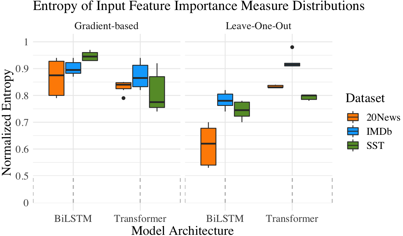
Figure 2: Entropy of gradient-based $\mathbf{g}_{\hat{y}}(\mathbf{x})$ and LOO $D_{\hat{y}}(\mathbf{x})$ FI distributions. Results are from models with full spectrum of projection functions.

Sparse Attention $\neq$ Sparse Input Feature Importance.

Our prior results demonstrated that—even when using sparse attention—we cannot identify a subset of influential inputs directly through intermediate representations; we explore whether a subset can still be identified through FI metrics. In the case where the normalized FI distribution highlights only a few key items, the distribution will, by definition, have low entropy. Thus, we explore whether sparse attention leads to lower entropy input FI distributions in comparison to standard attention. We find no such trend; Fig. 2 shows that across all models and settings, the entropy of the FI distribution is quite high. Further, we see a consistent negative correlation between this entropy and the sparsity parameter of the sparsegen projection (Table 2), implying that entropy of feature importance increases as we raise the degree of sparsity in ${\boldsymbol{\alpha}}$.

IMDb 20-News SST BiLSTM (tanh) -0.935 -0.675 -0.866 Transformer (dot) -0.830 -0.409 -0.810

Table 2: Correlation between sparsegen parameter² $\lambda$ and entropy of gradient-based input FI $\tilde{\mathrm{H}}(\mathbf{g}_{\hat{y}}(\mathbf{x}))$.

Correlation between Attention and Feature Importance.

Finally, we follow the experimental setup of Jain and Wallace (2019), who postulate that if the attention distribution indicates which inputs influence model behavior, then one may reasonably expect attention to correlate with FI measures of the input. While they find only a weak correlation, we explore how inducing sparsity in the attention distribution affects this result. Surprisingly, Fig. 3 shows a downward trend in this correlation as the sparsity parameter $\lambda$ of the sparsegen projection function is increased. As argued by Wiegreffe and Pinter (2019), a lack of this correlation does not indicate attention cannot be used as explanation; FI measures are not ground-truth indicators of critical inputs. However, the inverse relationship between input FI and attention is rather surprising. If anything, we may surmise sparsity in ${\boldsymbol{\alpha}}$ leads to less faithful explanations from ${\boldsymbol{\alpha}}$.

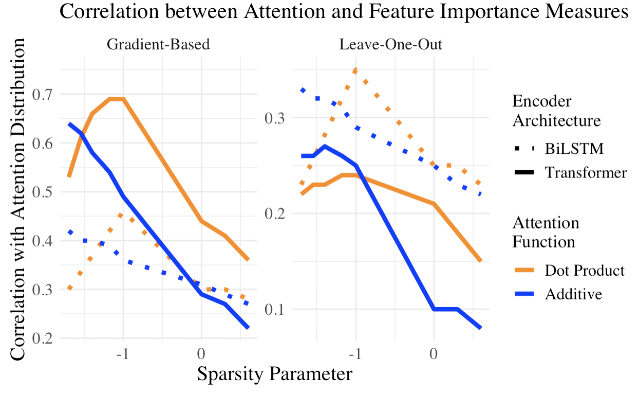
Figure 3: Correlation between the attention distribution and input FI measures as a function of the sparsity penalty $\lambda$ used in the projection function $\phi_{\mathrm{sparseg}}$. $x$-axis is log-scaled for $\lambda<0$ since $\lambda\in(-\infty,1)$. Results are from the IMDb dataset.

From these results, we posit that promoting sparsity in attention distribution may simply lead to the dispersion of information to different intermediate representations, a behavior similar to that seen when constraining attention for divergence from another distribution, i.e., in the adversarial experiments of Wiegreffe and Pinter (2019) compared to those of Jain and Wallace (2019).

5 Related Work

The use of attention as an indication of inputs’ influence on model decisions may at first seem natural; yet a large body of work has recently challenged this practice. Perhaps the first to do so was Jain and Wallace (2019), which revealed both a lack of correlation between the attention distribution and well established feature importance metrics and of unique optimal attention weights. Serrano and Smith (2019) contemporaneously found similar results. Subsequently, other studies arrived at similar results: for example, Grimsley et al. (2020) found evidence that causal explanations are not attainable from attention layers over text data; Pruthi et al. (2020) showed that attention masks can be trained to give deceptive explanations. We view this work as another such investigation, exploring attention’s innate interpretability on a different axis.

This work also fits into the context of a larger body of interpretability research in NLP, which has challenged the informal use of terms such as faithfulness, plausibility, and explainability (Lipton, 2018; Arrieta et al., 2020; Jacovi and Goldberg, 2021, inter alia) and tried to quantify the reliability of current definitions Atanasova et al. (2020a). While we consider these works in our experimental design—e.g., in our choice of FI metrics—we recognize that further experiments are needed to verify our findings: for example, similar experiments could be performed using the DeYoung et al. (2020) benchmark for evaluation; other FI metrics, such as selective attention Treviso and Martins (2020) should additionally be considered.author=ryan,color=violet!40,size=,fancyline,caption=,]Are you missing a period?

6 Conclusion

Prior work has cited interpretability as a driving factor for promoting sparsity in attention distributions. We explore how induced sparsity affects the ability to use attention as a tool for explaining model decisions. In our experiments on text classification tasks, we see that while sparse attention distributions may allow us to pinpoint influential intermediate representations, we are unable to find any plausible mapping from sparse attention to a small, critical set of influential inputs. Rather, we find evidence that inducing sparsity may make it even less plausible to use the attention distribution to interpret model behavior. We conclude that we need further reason to believe sparse attention increases model interpretability as our results do not support such claims.

Ethical Considerations

Machine learning models are being deployed in an increasing number of sensitive situations. In these settings, it is critical that models are interpretable, so that we can avoid e.g., inadvertent racial or gender bias. Giving a false sense of interpretability can allow models with undesirable (i.e., unethical or unstable) behavior to fly under the radar. We view this work as another critique of interpretability claims and hope our results will encourage the more careful consideration of interpretability assumptions when using machine learning models in practice.

Appendix A Feature Importance Metrics

author=clara,color=orange,size=,fancyline,caption=,]add in comment on norm here Notably, both inputs and intermediate representations are not single variables. Intermediate representations are $m$-dimensional vectors and inputs $\mathbf{x}$ are embedded as $X^{(e)}$, meaning each word $x_{i}$ is represented by a $d$-dimensional vector. Therefore, the gradient of $f$ w.r.t. individual inputs or intermediate representations will likewise be a $d$- (or $m$-) dimensional vector. To come up with a scalar estimate of feature importance, we take the $L_{2}$-norm of the evaluated gradient. Subsequently, we normalize over all $x_{i}$ (or $\mathbf{h}_{i})$ to calculate relative feature importance of individual $x_{i}$ (or $\mathbf{h}_{i})$. The discussed transformation can be mathematically formalized by Eq. 5 and 4. For intermediate representations, this computation measures the influence on the magnitude of $\mathbf{h}_{p}$ rather than on $\mathbf{h}_{p}$ itself. However, we also experimented with measuring the influence directly on each facet of $\mathbf{h}_{p}$, taking the magnitude of this vector. We found empirically that the two measures returned nearly identical results while measuring influence on magnitude was significantly more computationally efficient.

Appendix B Experimental Setup

We use exact datasets provided by and based our experimental framework on that of Jain and Wallace (2019), which can be found at https://github.com/successar/AttentionExplanation. For both comparison and reproducibility, we exactly follow their preprocessing steps, which are described in their paper. Source code, model statistics, and links to datasets can be found at the above link. In the experiments we use a Bidirectional LSTM encoder or a Transformer encoder which has 2 layers with 1 attention head. All hidden dimensions are set to $128$. The models and the training procedure have been implemented by using the PyTorch library Paszke et al. (2019). For training we use the Adam optimizer Kingma and Ba (2015) with the amsgrad Reddi et al. (2018) option enabled. Some important hyperparameters are listed in Table 4; minor tuning was performed in order to reach comparable performance with respect to Jain and Wallace (2019) and Wiegreffe and Pinter (2019). An important note regarding this table is that the listed learning rate and weight decay correspond to all model parameters except the ones specifically for the attention mechanism. The latter we train without a weight decay and with either the same or $10$x larger learning rate.

Train size Test size Accuracy (T) Accuracy (B) IMDb 25000 4356 0.89 0.90 20News 1426 334 0.91 0.91 SST 6355 1725 0.79 0.82

Table 3: Dataset statistics and baseline accuracy scores on test sets for Transformer with dot product attention (T) and BiLSTM with additive attention (B). All datasets are in english.

Batch Size Learning Rate Weight Decay LSTM 32 $1\times 10^{-4}$ $1\times 10^{-5}$ Transformer 32 $1\times 10^{-5}$ $1\times 10^{-5}$

Table 4: Hyperparameters used for training the models with LSTM and Transformer encoder respectively.

Appendix C Additional Results

C.1 Adversarial Experiments

IMDb SST 20News JSD Acc. JSD Acc. JSD Acc. BiLSTM (adv. frozen) 0.67 0.76 ​ ​- ​.14 0.62 0.76 ​ ​- ​.06 0.67 0.78 ​ ​- ​.13 BiLSTM (adv. unfrozen) 0.67 0.90 ​ ​- ​.00 0.61 0.82 ​ ​- ​.00 0.67 0.91 ​ ​- ​.00 Transformer (adv. frozen) 0.62 0.71 ​ ​- ​.18 0.57 0.76 ​ ​- ​.03 0.62 0.87 ​ ​- ​.03 Transformer (adv. unfrozen) 0.64 0.87 ​ ​- ​.02 0.57 0.78 ​ ​- ​.01 0.62 0.92 ​ ​$+$​ .01

Table 5: JSD (between original and adversarial attention distributions) and model accuracy on test sets. Colored numbers are differences from baseline. While Wiegreffe and Pinter (2019) present TVD, we present JSD as it is the metric being optimized over. Note that JSD is a lower-bound on TVD and should roughly show the same trends.

We construct adversarial attention distributions by optimizing for the divergence of the distribution from a baseline model’s attention distribution using two methods: (1) by transferring all model parameters of a pre-trained base model and optimizing for divergence (frozen) and (2) training an entirely new model and optimizing for divergence (unfrozen). We use Jensen-Shannon divergence (JSD) to measure the difference between the adversarial and baseline distributions. Table 5 shows that although we can attain high JSD under both methods, the former leads to a large drop in performance. If we believe the model must encode the same information to achieve similar accuracy, the difference in accuracies of the two methods implies that in the first method, the model likely redistributes information across encoder outputs.

C.2 Correlation between Attention Distribution and Inputs/Intermediate Representations

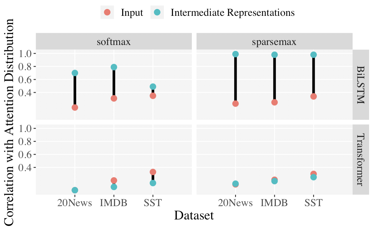
Figure 4: Correlation between the attention distribution and Leave-One_Out FI measures. We see a stronger correlation between attention and intermediate representation FI than input FI across all models.

We provide the full results of our experiments on correlation of the input and intermediate representations with the attention distribution in Table 6.

IMDb 20-News SST $\mathbf{g}_{\hat{y}}(\mathbf{x})$ $D_{\hat{y}}(\mathbf{x})$ $\mathbf{g}_{\hat{y}}(\mathbf{x})$ $D_{\hat{y}}(\mathbf{x})$ $\mathbf{g}_{\hat{y}}(\mathbf{x})$ $D_{\hat{y}}(\mathbf{x})$ BiLSTM Softmax 0.36 ​ ​$\pm$ 0.12 0.31 ​ ​$\pm$ 0.08 0.24 ​ ​$\pm$ 0.24 0.17 ​ ​$\pm$ 0.17 0.25 ​ ​$\pm$ 0.28 0.35 ​ ​$\pm$ 0.18 BiLSTM Sparsemax 0.31 ​ ​$\pm$ 0.08 0.25 ​ ​$\pm$ 0.06 0.25 ​ ​$\pm$ 0.13 0.23 ​ ​$\pm$ 0.09 0.45 ​ ​$\pm$ 0.13 0.34 ​ ​$\pm$ 0.15 Transformer Softmax 0.67 ​ ​$\pm$ 0.08 0.20 ​ ​$\pm$ 0.10 0.54 ​ ​$\pm$ 0.11 0.05 ​ ​$\pm$ 0.10 0.72 ​ ​$\pm$ 0.11 0.33 ​ ​$\pm$ 0.20 Transformer Sparsemax 0.44 ​ ​$\pm$ 0.08 0.21 ​ ​$\pm$ 0.09 0.47 ​ ​$\pm$ 0.10 0.14 ​ ​$\pm$ 0.15 0.67 ​ ​$\pm$ 0.12 0.30 ​ ​$\pm$ 0.23 $\mathbf{g}_{\hat{y}}(I)$ $D_{\hat{y}}(I)$ $\mathbf{g}_{\hat{y}}(I)$ $D_{\hat{y}}(I)$ $\mathbf{g}_{\hat{y}}(I)$ $D_{\hat{y}}(I)$ BiLSTM Softmax 0.77 ​ ​$\pm$ 0.05 0.79 ​ ​$\pm$ 0.05 0.78 ​ ​$\pm$ 0.15 0.70 ​ ​$\pm$ 0.19 0.80 ​ ​$\pm$ 0.13 0.49 ​ ​$\pm$ 0.17 BiLSTM Sparsemax 0.98 ​ ​$\pm$ 0.02 0.98 ​ ​$\pm$ 0.02 0.98 ​ ​$\pm$ 0.06 0.99 ​ ​$\pm$ 0.01 0.97 ​ ​$\pm$ 0.06 0.98 ​ ​$\pm$ 0.04 Transformer Softmax 0.76 ​ ​$\pm$ 0.04 0.1 ​ ​$\pm$ 0.07 0.62 ​ ​$\pm$ 0.13 0.05 ​ ​$\pm$ 0.11 0.89 ​ ​$\pm$ 0.07 0.16 ​ ​$\pm$ 0.18 Transformer Sparsemax 0.92 ​ ​$\pm$ 0.05 0.19 ​ ​$\pm$ 0.09 0.76 ​ ​$\pm$ 0.15 0.15 ​ ​$\pm$ 0.16 0.88 ​ ​$\pm$ 0.11 0.25 ​ ​$\pm$ 0.23

Table 6: Mean Kendall’s $\tau$ correlation of attention with gradient-based $\mathbf{g}_{\hat{y}}$ and LOO-based $D_{\hat{y}}$ feature importance of the input tokens $\mathbf{x}$ and intermediate representations $I$. Green numbers are standard deviations.

References

- Arrieta et al. (2020) Alejandro Barredo Arrieta, Natalia Díaz-Rodríguez, Javier Del Ser, Adrien Bennetot, Siham Tabik, Alberto Barbado, Salvador García, Sergio Gil-López, Daniel Molina, Richard Benjamins, Raja Chatila, and Francisco Herrera. 2020. Explainable Artificial Intelligence (XAI): Concepts, Taxonomies, Opportunities and Challenges toward Responsible AI. Information Fusion, 58.
- Atanasova et al. (2020a) Pepa Atanasova, Jakob Grue Simonsen, Christina Lioma, and Isabelle Augenstein. 2020a. A diagnostic study of explainability techniques for text classification. In Proceedings of the 2020 Conference on Empirical Methods in Natural Language Processing (EMNLP), pages 3256–3274, Association for Computational Linguistics.
- Atanasova et al. (2020b) Pepa Atanasova, Jakob Grue Simonsen, Christina Lioma, and Isabelle Augenstein. 2020b. Generating fact checking explanations. In Proceedings of the 58th Annual Meeting of the Association for Computational Linguistics, pages 7352–7364, Association for Computational Linguistics.
- Baehrens et al. (2010) David Baehrens, Timon Schroeter, Stefan Harmeling, Motoaki Kawanabe, Katja Hansen, and Klaus-Robert Müller. 2010. How to explain individual classification decisions. Journal of Machine Learning Research, 11:1803–1831.
- Bahdanau et al. (2015) Dzmitry Bahdanau, Kyunghyun Cho, and Yoshua Bengio. 2015. Neural machine translation by jointly learning to align and translate. In 3rd International Conference on Learning Representations.
- Brunner et al. (2020) Gino Brunner, Yang Liu, Damián Pascual, Oliver Richter, Massimiliano Ciaramita, and Roger Wattenhofer. 2020. On identifiability in Transformers. In 8th International Conference on Learning Representations.
- Camburu et al. (2018) Oana-Maria Camburu, Tim Rocktäschel, Thomas Lukasiewicz, and Phil Blunsom. 2018. e-SNLI: Natural Language Inference with Natural Language Explanations. In Advances in Neural Information Processing Systems 31, pages 9539–9549. Curran Associates, Inc.
- Carton et al. (2020) Samuel Carton, Anirudh Rathore, and Chenhao Tan. 2020. Evaluating and characterizing human rationales. In Proceedings of the 2020 Conference on Empirical Methods in Natural Language Processing (EMNLP), pages 9294–9307, Association for Computational Linguistics.
- De-Arteaga et al. (2019) Maria De-Arteaga, Alexey Romanov, Hanna Wallach, Jennifer Chayes, Christian Borgs, Alexandra Chouldechova, Sahin Geyik, Krishnaram Kenthapadi, and Adam Tauman Kalai. 2019. Bias in bios: A case study of semantic representation bias in a high-stakes setting. In Proceedings of the Conference on Fairness, Accountability, and Transparency, page 120–128, Association for Computing Machinery.
- DeYoung et al. (2020) Jay DeYoung, Sarthak Jain, Nazneen Fatema Rajani, Eric Lehman, Caiming Xiong, Richard Socher, and Byron C. Wallace. 2020. ERASER: A benchmark to evaluate rationalized NLP models. In Proceedings of the 58th Annual Meeting of the Association for Computational Linguistics, pages 4443–4458, Association for Computational Linguistics.
- Doshi-Velez and Kim (2017) Finale Doshi-Velez and Been Kim. 2017. Towards a rigorous science of interpretable machine learning. CoRR, abs/1702.08608.
- Gehrmann et al. (2019) Sebastian Gehrmann, Hendrik Strobelt, Robert Krueger, Hanspeter Pfister, and Alexander M Rush. 2019. Visual interaction with deep learning models through collaborative semantic inference. IEEE Transactions on Visualization and Computer Graphics, 26(1):884–894.
- Grimsley et al. (2020) Christopher Grimsley, Elijah Mayfield, and Julia R.S. Bursten. 2020. Why attention is not explanation: Surgical intervention and causal reasoning about neural models. In Proceedings of the 12th Language Resources and Evaluation Conference, pages 1780–1790, European Language Resources Association.
- Guidotti et al. (2018) Riccardo Guidotti, Anna Monreale, Salvatore Ruggieri, Franco Turini, Fosca Giannotti, and Dino Pedreschi. 2018. A survey of methods for explaining black box models. ACM Computing Surveys, 51(5).
- Jacovi and Goldberg (2020) Alon Jacovi and Yoav Goldberg. 2020. Towards faithfully interpretable NLP systems: How should we define and evaluate faithfulness? In Proceedings of the 58th Annual Meeting of the Association for Computational Linguistics, pages 4198–4205, Association for Computational Linguistics.
- Jacovi and Goldberg (2021) Alon Jacovi and Yoav Goldberg. 2021. Aligning Faithful Interpretations with their Social Attribution. Transactions of the Association for Computational Linguistics, 9:294–310.
- Jain and Wallace (2019) Sarthak Jain and Byron C. Wallace. 2019. Attention is not Explanation. In Proceedings of the 2019 Conference of the North American Chapter of the Association for Computational Linguistics: Human Language Technologies, Volume 1 (Long and Short Papers), pages 3543–3556, Association for Computational Linguistics.
- Kingma and Ba (2015) Diederik P. Kingma and Jimmy Ba. 2015. Adam: A method for stochastic optimization. In 3rd International Conference on Learning Representations.
- Knight (1966) William R. Knight. 1966. A computer method for calculating Kendall’s tau with ungrouped data. Journal of the American Statistical Association, 61(314):436–439.
- Kotonya and Toni (2020) Neema Kotonya and Francesca Toni. 2020. Explainable automated fact-checking: A survey. In Proceedings of the 28th International Conference on Computational Linguistics, pages 5430–5443, International Committee on Computational Linguistics.
- Laha et al. (2018) Anirban Laha, Saneem Ahmed Chemmengath, Priyanka Agrawal, Mitesh Khapra, Karthik Sankaranarayanan, and Harish G Ramaswamy. 2018. On controllable sparse alternatives to softmax. In Advances in Neural Information Processing Systems 31, pages 6422–6432. Curran Associates, Inc.
- Lipton (2018) Zachary C. Lipton. 2018. The mythos of model interpretability. Queue, 16(3):31–57.
- Malaviya et al. (2018) Chaitanya Malaviya, Pedro Ferreira, and André F. T. Martins. 2018. Sparse and constrained attention for neural machine translation. In Proceedings of the 56th Annual Meeting of the Association for Computational Linguistics (Volume 2: Short Papers), pages 370–376, Association for Computational Linguistics.
- Martins and Astudillo (2016) Andre Martins and Ramon Astudillo. 2016. From softmax to sparsemax: A sparse model of attention and multi-label classification. In Proceedings of The 33rd International Conference on Machine Learning, volume 48 of Proceedings of Machine Learning Research, pages 1614–1623.
- Miller (2019) Tim Miller. 2019. Explanation in artificial intelligence: Insights from the social sciences. Artificial Intelligence, 267:1–38.
- Ming et al. (2017) Y. Ming, S. Cao, R. Zhang, Z. Li, Y. Chen, Y. Song, and H. Qu. 2017. Understanding hidden memories of recurrent neural networks. In 2017 IEEE Conference on Visual Analytics Science and Technology, pages 13–24.
- Mullenbach et al. (2018) James Mullenbach, Sarah Wiegreffe, Jon Duke, Jimeng Sun, and Jacob Eisenstein. 2018. Explainable prediction of medical codes from clinical text. In Proceedings of the 2018 Conference of the North American Chapter of the Association for Computational Linguistics: Human Language Technologies, Volume 1 (Long Papers), pages 1101–1111, Association for Computational Linguistics.
- Niculae et al. (2018) Vlad Niculae, André Martins, Mathieu Blondel, and Claire Cardie. 2018. SparseMAP: Differentiable sparse structured inference. In Proceedings of the 35th International Conference on Machine Learning, volume 80, pages 3799–3808.
- Paszke et al. (2019) Adam Paszke, Sam Gross, Francisco Massa, Adam Lerer, James Bradbury, Gregory Chanan, Trevor Killeen, Zeming Lin, Natalia Gimelshein, Luca Antiga, Alban Desmaison, Andreas Kopf, Edward Yang, Zachary DeVito, Martin Raison, Alykhan Tejani, Sasank Chilamkurthy, Benoit Steiner, Lu Fang, Junjie Bai, and Soumith Chintala. 2019. Pytorch: An imperative style, high-performance deep learning library. In Advances in Neural Information Processing Systems 32, pages 8024–8035. Curran Associates, Inc.
- Peters et al. (2019) Ben Peters, Vlad Niculae, and André F. T. Martins. 2019. Sparse sequence-to-sequence models. In Proceedings of the 57th Annual Meeting of the Association for Computational Linguistics, pages 1504–1519, Association for Computational Linguistics.
- Poerner et al. (2018) Nina Poerner, Hinrich Schütze, and Benjamin Roth. 2018. Evaluating neural network explanation methods using hybrid documents and morphosyntactic agreement. In Proceedings of the 56th Annual Meeting of the Association for Computational Linguistics (Volume 1: Long Papers), pages 340–350, Association for Computational Linguistics.
- Pruthi et al. (2020) Danish Pruthi, Mansi Gupta, Bhuwan Dhingra, Graham Neubig, and Zachary C. Lipton. 2020. Learning to deceive with attention-based explanations. In Proceedings of the 58th Annual Meeting of the Association for Computational Linguistics, pages 4782–4793, Association for Computational Linguistics.
- Reddi et al. (2018) Sashank J. Reddi, Satyen Kale, and Sanjiv Kumar. 2018. On the convergence of Adam and beyond. In 6th International Conference on Learning Representations.
- Rudin (2019) Cynthia Rudin. 2019. Stop explaining black box machine learning models for high stakes decisions and use interpretable models instead. Nature Machine Intelligence, 1(5):206–215.
- Salehinejad et al. (2017) Hojjat Salehinejad, Sharan Sankar, Joseph Barfett, Errol Colak, and Shahrokh Valaee. 2017. Recent advances in recurrent neural networks. CoRR, abs/1801.01078.
- Serrano and Smith (2019) Sofia Serrano and Noah A. Smith. 2019. Is attention interpretable? In Proceedings of the 57th Annual Meeting of the Association for Computational Linguistics, pages 2931–2951, Association for Computational Linguistics.
- Simonyan et al. (2014) Karen Simonyan, Andrea Vedaldi, and Andrew Zisserman. 2014. Deep inside convolutional networks: Visualising image classification models and saliency maps. In 2nd International Conference on Learning Representations.
- Sutskever et al. (2014) Ilya Sutskever, Oriol Vinyals, and Quoc V. Le. 2014. Sequence to sequence learning with neural networks. In Advances in Neural Information Processing Systems 27, pages 3104–3112. Curran Associates, Inc.
- Treviso and Martins (2020) Marcos Treviso and André F. T. Martins. 2020. The explanation game: Towards prediction explainability through sparse communication. In Proceedings of the Third BlackboxNLP Workshop on Analyzing and Interpreting Neural Networks for NLP, pages 107–118, Association for Computational Linguistics.
- Tu et al. (2016) Zhaopeng Tu, Zhengdong Lu, Yang Liu, Xiaohua Liu, and Hang Li. 2016. Modeling coverage for neural machine translation. In Proceedings of the 54th Annual Meeting of the Association for Computational Linguistics (Volume 1: Long Papers), pages 76–85, Association for Computational Linguistics.
- Tutek and Snajder (2020) Martin Tutek and Jan Snajder. 2020. Staying true to your word: (how) can attention become explanation? In Proceedings of the 5th Workshop on Representation Learning for NLP, pages 131–142, Association for Computational Linguistics.
- Wiegreffe and Pinter (2019) Sarah Wiegreffe and Yuval Pinter. 2019. Attention is not not explanation. In Proceedings of the 2019 Conference on Empirical Methods in Natural Language Processing and the 9th International Joint Conference on Natural Language Processing (EMNLP-IJCNLP), pages 11–20, Association for Computational Linguistics.
- Xie et al. (2017) Qizhe Xie, Xuezhe Ma, Zihang Dai, and Eduard Hovy. 2017. An interpretable knowledge transfer model for knowledge base completion. In Proceedings of the 55th Annual Meeting of the Association for Computational Linguistics (Volume 1: Long Papers), pages 950–962, Association for Computational Linguistics.
- Yang et al. (2016) Zichao Yang, Diyi Yang, Chris Dyer, Xiaodong He, Alex Smola, and Eduard Hovy. 2016. Hierarchical attention networks for document classification. In Proceedings of the 2016 Conference of the North American Chapter of the Association for Computational Linguistics: Human Language Technologies, pages 1480–1489, Association for Computational Linguistics.
- Zhang et al. (2019) J. Zhang, Y. Zhao, H. Li, and C. Zong. 2019. Attention with sparsity regularization for neural machine translation and summarization. IEEE/ACM Transactions on Audio, Speech, and Language Processing, 27(3):507–518.