Plasma Properties, Switchback Patches and Low $\alpha$-Particle Abundance in Slow Alfvénic Coronal Hole Wind at 0.13 au

Abstract

The Parker Solar Probe (PSP) mission presents a unique opportunity to study the near-Sun solar wind closer than any previous spacecraft. During its fourth and fifth solar encounters, PSP had the same orbital trajectory, meaning that solar wind was measured at the same latitudes and radial distances. We identify two streams measured at the same heliocentric distance ($\sim$0.13au) and latitude ($\sim$-3.5^∘) across these encounters to reduce spatial evolution effects. By comparing the plasma of each stream, we confirm that they are not dominated by variable transient events, despite PSP’s proximity to the heliospheric current sheet. Both streams are consistent with a previous slow Alfvénic solar wind study once radial effects are considered, and appear to originate at the Southern polar coronal hole boundary. We also show that the switchback properties are not distinctly different between these two streams. Low $\alpha$-particle abundance ($\sim$ 0.6 %) is observed in the encounter 5 stream, suggesting that some physical mechanism must act on coronal hole boundary wind to cause $\alpha$-particle depletion. Possible explanations for our observations are discussed, but it remains unclear whether the depletion occurs during the release or the acceleration of the wind. Using a flux tube argument, we note that an $\alpha$-particle abundance of $\sim$ 0.6 % in this low velocity wind could correspond to an abundance of $\sim$ 0.9 % at 1 au. Finally, as the two streams roughly correspond to the spatial extent of a switchback patch, we suggest that patches are distinct features of coronal hole wind.

1 Introduction

The solar wind, which is usually categorised as either fast ($>600$km/s) or slow ($<400$km/s) based on its bulk velocity, comprises ions and electrons that stream out into interplanetary space. Protons are by far the most dominant ion species, but the plasma also contains populations of doubly-ionised helium ($\alpha$-particles) and heavier ions. It is widely accepted that the source of the fast solar wind is coronal holes (Krieger et al., 1973; Nolte et al., 1976; Sheeley et al., 1976; Neugebauer et al., 1998), but the origin of the more variable slow solar wind (Bame et al., 1977) is still unclear. Slow solar wind could come from coronal hole boundaries at solar minimum (Wang & Sheeley, 1994; Neugebauer et al., 1998), and from small coronal holes (Wang & Sheeley, 1994; Neugebauer et al., 1998) and/or active regions at solar maximum (Neugebauer et al., 2002; Harra et al., 2008).

Part of the issue with identifying the sources of the slow wind arises because of this binary classification based purely on bulk velocity. Many studies have therefore tried to improve upon the current solar wind categorisation (e.g. Xu & Borovsky, 2015; Camporeale et al., 2017; Li et al., 2020). Recent work by D’Amicis & Bruno (2015) suggests that there are at least two modes of slow solar wind: an Alfvénic population and a non-Alfvénic population. The Alfvénic slow wind has similar properties to the fast wind (D’Amicis et al., 2019; Perrone et al., 2020; Stansby et al., 2020b), which indicates that it may also originate in coronal holes or at their boundaries (D’Amicis & Bruno, 2015). The non-Alfvénic slow wind is associated with highly variable mass fluxes (Stansby et al., 2019a), which is consistent with wind from active regions (D’Amicis & Bruno, 2015) or transients related to coronal streamers (Einaudi et al., 1999; D’Amicis & Bruno, 2015; Stansby et al., 2019a). However, more studies are needed to fully characterise different solar wind streams as the sources and formation mechanisms of slow wind are still actively debated (Abbo et al., 2016). The recent launch of the Parker Solar Probe (PSP; Fox et al. (2016)) mission provides a novel data set for these studies.

To date, PSP has remained at low latitudes during solar minimum and predominantly observed slow solar wind. PSP has routinely measured switchbacks - rotations of the magnetic field away from its background orientation - in this slow wind (Bale et al., 2019; Kasper et al., 2019), but switchbacks have also been previously observed in fast solar wind by Helios (Horbury et al., 2018) and Ulysses (Neugebauer & Goldstein, 2013). Switchbacks appear to occur in groups or ‘patches’ which are separated by more radial ‘quiet’ intervals close to the Sun (Horbury et al., 2020). While many studies have looked at the properties of switchbacks including their shape and size (Laker et al., 2020), their temperature (Woolley et al., 2020; Woodham et al., 2020) and their occurrence rate and duration (Dudok de Wit et al., 2020), the mechanisms that cause switchbacks are still actively debated. It has been suggested that magnetic field switchbacks could be related to solar wind origins. For example, switchbacks may be caused by interchange reconnection (Zank et al., 2020), mini-filament eruption (Sterling & Moore, 2020) or Alfvén-wave turbulence (Squire et al., 2020; Shoda et al., 2021), meaning that studies of these events could help to disentangle the physical processes governing the solar wind release.

The $\alpha$-particle (or helium) abundance ($A_{\alpha}$) - the ratio of $\alpha$-particle to proton number density - is another feature that is highly influenced by solar source regions. On average, the $\alpha$-particle abundance in the solar wind is between 3% and 6% (Ogilvie & Wilkerson, 1969; Robbins et al., 1970; Neugebauer, 1981; Alterman et al., 2021), but can increase to over 15% during solar flares (Hirshberg et al., 1972a). At solar minimum, the $\alpha$-particle abundance is higher (Hirshberg et al., 1972b; Kasper et al., 2007, 2012) and more stable (Bame et al., 1977; Feldman et al., 1978) in the fast solar wind ($A_{\alpha}\sim$ 4-5%) than in the slow wind ($A_{\alpha}\sim$ 1-2%). However, this velocity dependence does not persist during solar maximum, where the slow and fast wind have comparable $\alpha$-particle abundances of $\sim$ 4-5% (Kasper et al., 2007, 2012). Recent work by Huang et al. (2020) shows that highly Alfvénic slow solar wind contains both helium poor ($A_{\alpha}\sim$ 1.5 %) and helium rich ($A_{\alpha}\sim$ 4.5 %) populations, suggesting multiple solar sources for this type of wind. They also show that some slow solar wind plasma properties are similar regardless of Alfvénicity, which could indicate commonality in the source regions of all slow solar wind.

A crucial step to understanding the sources and release of solar wind plasma involves identifying the properties of different solar wind types closer to the Sun. Here we take advantage of the fact that PSP had the same orbital trajectory during encounters 4 and 5 to identify two streams of slow Alfvénic coronal hole wind measured at the same latitude and radius during solar minimum. We compare the proton and $\alpha$-particle parameters before presenting the conditions of this slow Alfvénic wind closer than any previous study. In Section 3.3.1, we analyse switchback statistics for each interval. We present $\alpha$-particle data for one stream, showing that the $\alpha$-particle abundance is very low and justifying why such low abundance is not seen at 1 au. These results are then discussed in relation to solar wind sources in Section 4.2.

2 Data

The data used here were measured by PSP (Fox et al., 2016) during its fourth and fifth encounters. The magnetic field data were measured by the flux-gate magnetometer (MAG) from the FIELDS instrument suite (Bale et al., 2016).

We use proton core parameters (i.e. velocity, parallel temperature, perpendicular temperature and density) derived from the ion distribution functions measured by the SPAN-I instrument (Kasper et al., 2016). We fit a two population bi-Maxwellian to the 3D proton distribution functions as detailed in Finley et al. (2020) (For alternatives see e.g. Stansby et al., 2018; Woodham et al., 2020). In the presence of Alfvénic fluctuations, the proton core and beam populations rotate in velocity space (Matteini et al., 2014, 2015a) and can move out of the instrument’s limited field of view (Woodham et al., 2020), making measurements of these populations unreliable under certain plasma conditions. For the intervals studied here we focus only on the proton core as this is more steadily within the field of view than the proton beam. The $\alpha$-particles, which are approximately stationary in velocity space under Alfvénic fluctuations (Matteini et al., 2015a), were fit using a bi-Maxwellian after removing proton contamination from the $\alpha$-particle channel as in Finley et al. (2020). The encounter 4 $\alpha$-particle data have been disregarded here because unusually low counts in the instrument resulted in less reliable fits.

We use strahl electron parallel temperature ($T_{strahl,\parallel}$) as an estimate for the coronal electron temperature at the source (Berčič et al., 2020). To obtain this parameter we fit the electron velocity distribution functions (VDFs) measured by SPAN-E instrument (Kasper et al., 2016; Whittlesey et al., 2020). We perform the fits in the magnetic field aligned, plasma rest frame, which is defined with the magnetic field vector from MAG and the velocity moment derived from the SPAN-I proton distribution functions. We model the parallel cut through the strahl distribution function with a non-drifting 1D Maxwellian, from which we obtain $T_{strahl,\parallel}$. According to the collisionless exospheric models (Jockers, 1970; Lemaire & Scherer, 1970, 1971; Maksimovic et al., 1997) this temperature does not change during the solar wind expansion and can therefore give a good estimate of the electron temperature in the solar corona. The fitting method includes an additional step to correct for the portion of the SPAN-E field-of-view blocked by the PSP’s heat shield, which is further described in Sec. 3.1 of Berčič et al. (2020).

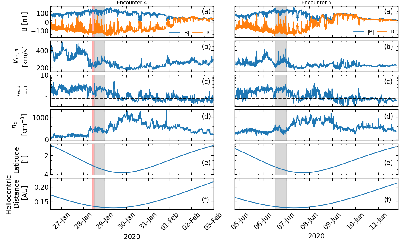
Figure 1: Time series of PSP’s encounter 4 (left) and encounter 5 (right). The panels show: (a) magnitude and radial component of the magnetic field, (b) proton core radial velocity, (c) proton core temperature anisotropy, (d) total proton number density, (e) latitude and (f) heliocentric distance. The grey shaded regions show the two streams analysed in this study. The red shaded region shows the ‘quiet’ interval used for comparison in this study. The dashed black line in panel (c) shows where the temperature anisotropy is unity.

3 Results

3.1 Identification of Two Streams

In order to reduce spatial effects, we manually choose two streams across PSP’s fourth and fifth encounters such that the solar wind was measured at the same latitude and radius in each. Fig. 1 shows time series data from encounters 4 (left) and 5 (right), with the two intervals used in this study shaded grey (referred to now on as the E4 and E5 streams, respectively). Panel (a) shows the magnitude and the radial component of the magnetic field, which appears to be modulated into ‘patches’ of switchbacks separated by ‘quiet’ solar wind (Bale et al., 2019; Horbury et al., 2020). This ‘quiet’ solar wind (referred to as quiet intervals or periods henceforth) has been shown to contain large proton beams and significant wave activity (Verniero et al., 2020). The red shaded region is a ‘quiet’ period and is used as a comparison interval to the two streams identified. Due to the high Alfvénicity of the solar wind close to the Sun, the proton core radial velocity, which is $\sim$ 300 km/s in the two streams, also appears in patches (panel b). Panels (c) and (d) show the proton core anisotropy and the proton density, respectively. During PSP’s outbound journey for each encounter, the density is enhanced and the anisotropy reduced compared to the same radius on the inbound journey. This is because of the proximity of PSP to the heliospheric current sheet (HCS) and the heliospheric plasma sheet (HPS), where slower and more dense wind is found. Panels (e) and (f) show that both streams were measured at $\sim$-3.5^∘ latitude and $\sim$0.13 au, just before perihelion.

3.2 Comparison of the Streams

3.2.1 Plasma Properties

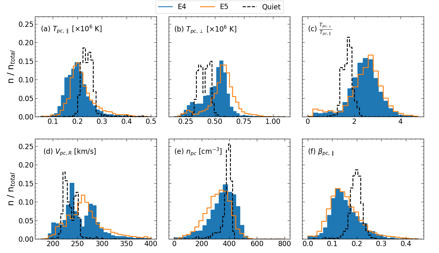
Figure 2: Histograms of proton core parameters during the E4 (blue), E5 (orange) and quiet (black) streams. The panels show: (a) parallel temperature, (b) perpendicular temperature, (c) temperature anisotropy, (d) radial velocity, (e) number density and (f) plasma $\beta_{\parallel}$.

Fig. 2 shows distributions of proton core parameters for the two streams identified in Section 3.1. The panels show: (a) parallel temperature, (b) perpendicular temperature, (c) temperature anisotropy, (d) radial velocity, (e) number density and (f) plasma $\beta_{\parallel}$. The neighbouring interval of ‘quiet’ wind (see red shaded interval in Fig. 1) measured at a similar radius, latitude and time is also shown here.

Overall, the proton core distributions in the E4 and E5 streams are remarkably similar to each other for solar wind measured 5 months apart. The perpendicular temperature distributions show the largest difference with the E5 stream $\sim 13\%$ hotter on average than the E4 stream. This is most likely caused by the solar wind temperature-velocity relationship (Burlaga & Ogilvie, 1970; Lopez & Freeman, 1986), as the E5 stream is, on average, $\sim 5\%$ faster than the E4 stream. This velocity difference could also explain the slightly lower density in the E5 stream as faster wind is less dense than slower wind (Verscharen et al., 2019). In contrast, the parallel temperature distributions are very similar and peak at $\sim 0.2\times 10^{6}$K. This could indicate that parallel temperature is less strongly dependent on velocity than the perpendicular temperature, as previously predicted for fast solar wind at 35$R_{S}$ (Perrone et al., 2019). Finally, the temperature anisotropy and $\beta_{pc,\parallel}$ distributions show no significant differences and peak at $\sim 2.5$ and $\sim 0.1$ for both streams. Some of the quiet interval parameters deviate significantly from the E4 and E5 streams. For example, the perpendicular temperature is considerably lower and the parallel temperature is higher, leading to a smaller anisotropy. The ‘quiet’ period radial velocity and density distributions are similar to, but more strongly peaked than, the corresponding E4 and E5 stream distributions. $\beta_{pc,\parallel}$ in the ‘quiet’ interval is almost twice as large as in the E4 and E5 streams.

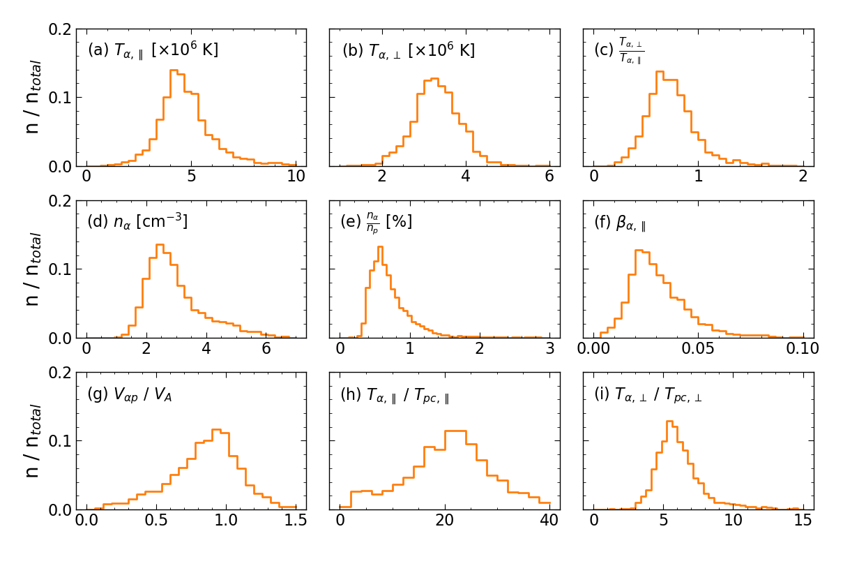
Figure 3: Histograms of $\alpha$-particle parameters during the E5 stream. The panels show: (a) parallel temperature, (b) perpendicular temperature, (c) temperature anisotropy, (d) number density, (e) $\alpha$-particle abundance, (f) plasma $\beta_{\parallel}$, (g) normalised $\alpha$-proton drift, (h) $\alpha$-proton parallel temperature ratio and (i) $\alpha$-proton perpendicular temperature ratio.

Fig. 3 shows distributions of the E5 stream $\alpha$-particle parameters. Panels (a) and (b) show that the $\alpha$-particles have parallel and perpendicular temperatures of $\sim$ 4.5$\times$10⁶K and $\sim$ 3.5$\times$10⁶K, respectively. The $\alpha$-particles are considerably hotter than the protons here. The $\alpha$-to-proton temperature ratios are $\sim$ 20-25 and $\sim$ 6 for parallel and perpendicular, respectively (panels (h) and (i)). Such a large parallel ratio may seem nonphysical, but it is a consequence of protons and $\alpha$-particles having opposite anisotropy. Panel (c) shows that the $\alpha$-particles, in contrast to the protons, have a temperature anisotropy less than one. The density of $\alpha$-particles is $\sim$ 3cm^-3 (panel d), which gives a remarkably low abundance (panel e). This is discussed in detail in Section 4.2. Panel (f) shows $\beta_{\alpha,\parallel}$ is $\sim$ 0.025, an order of magnitude less than protons. Panel (g) shows that the $\alpha$-particles, like in coronal hole fast wind, drift at a large fraction of the Alfvén speed ahead of the proton core population.

3.3 Type of Solar Wind and Source Region

As our comparisons suggest that the solar wind in the E4 and E5 streams is quantitatively similar, we conclude that this wind is unlikely to be caused by transient events which tend to be much more variable. We therefore try to establish the solar source of these solar wind streams.

Power spectra of the magnetic field fluctuations for each stream show power laws of -3/2 in the inertial range (not shown here). This is consistent with the scaling of non-HPS solar wind previously shown by Chen et al. (2021) using a similar encounter 4 stream. The -3/2 power law is also consistent with solar wind from the small equatorial coronal hole in encounter 1 (Bale et al., 2019; Chen et al., 2020). Conversely, the wind measured during the outbound sections of the encounters has an inertial range power law of -5/3 (Chen et al., 2021). The wind during this time was slower and more dense, consistent with predominantly HPS wind. We conclude that the chosen streams, measured on the inbound section of each encounter, are non-HPS solar wind from a coronal hole.

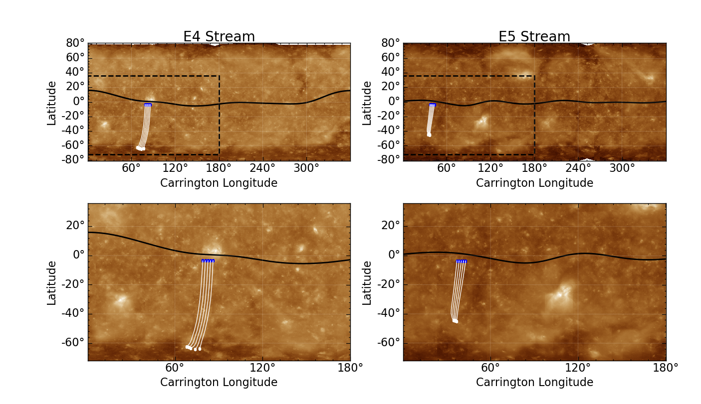
Figure 5: Potential field source surface mapping for the encounter 4 (left) and encounter 5 (right) streams. The top row shows the whole Sun and the bottom row shows a close up of the area of interest for each stream (indicated by the black dashed box in the top row). The white lines show the mapping of the magnetic field lines from the solar surface (white points) to the source surface (blue points). The solid black line shows the heliospheric current sheet. Both streams map to the edge of the Southern polar coronal hole.

Further evidence to support our conclusion is obtained by estimating the solar source region. The two solar wind streams are ballistically mapped to the source surface before a potential field source surface (PFSS) model (Altschuler & Newkirk, 1969; Schatten et al., 1969) is applied, using the pfsspy library (Stansby et al., 2020a), to determine solar origins of the wind (For other studies that use PFSS mapping see e.g. Badman et al., 2020; Laker et al., 2021; O’Kane et al., 2021). Both streams originate at the boundaries of the Southern polar coronal hole, separated by $\sim$30^∘ in longitude, according to the model (See Fig. 5 in Appendix. A). While this mapping is consistent with the in situ measured polarity, PSP is located very close to the HCS in both streams and so additional evidence to support the mapping and rule out streamer belt contributions is desirable. Considering this mapping with the high $\alpha$-proton drift (See Fig. 3) - a property of fast solar wind (Berger et al., 2011; Alterman et al., 2018) which is often linked to coronal hole source regions - further suggests that this slow wind originates from the boundaries of the Southern polar coronal hole.

Finally, Fig. 4 shows the strahl electron parallel temperature for each stream. As the strahl electrons propagate out of the corona with very little interaction with thermal distributions, this can be used as a proxy for the source temperature (Berčič et al., 2020). For the two streams, the strahl parallel temperature exhibits statistically similar distributions that peak around 1.1 $\times$10⁶K, suggesting that the two streams originated in regions with similar local plasma temperatures. By combining the above results with the low velocity of the wind, we suggest that the two streams contain slow Alfvénic coronal hole boundary wind from similar temperature source regions.

Table 1 shows a comparison of the slow Alfvénic wind at 0.13 au and at 0.35 au (Stansby et al., 2020b). The largest difference between the two studies is seen in the radial velocity, with the wind at 0.13 au being $\sim$ 100 km/s slower. There is also a larger proton anisotropy at 0.13 au, which is due to the radial evolution of temperature with distance from the Sun. The normalised $\alpha$-proton drift is larger closer to the Sun, while the proton flux and $\alpha$-particle anisotropy are similar at the two radial distances. The $\alpha$-proton temperature ratios are not markedly different in the two studies. These results are discussed further in Section 4.

Quantity	This Study	Stansby et al. (2020b)
Radius [au]	0.13	0.35
$V_{pc,R}$ [km/s]	$\sim$250 - 270	$\sim$380
$n_{p}V_{pc,R}r^{2}$ [$10^{35}s^{-1}sr^{-1}$]	$\sim$0.5	$\sim$0.6
Proton Anisotropy	$\sim$2-3	$\sim$1-2
$\alpha$-proton $T_{\perp}$ ratio	$\sim$6	$\sim$4
$\alpha$-proton $T_{\parallel}$ ratio	$\sim$20-25	$\sim$20
Normalised $\alpha$-proton Drift	$\sim$0.9	$\sim$0.5
$\alpha$ Anisotropy	$\sim$0.5-0.6	$\sim$0.6-0.7

Table 1: Peak distribution values of slow Alfvénic wind parameters from this study and Stansby et al. (2020b).

3.3.1 Switchbacks

Table 2 summarises the statistical properties of the switchbacks in each stream (the quiet interval has not been included as, by definition, quiet intervals have very few switchbacks). Switchbacks were identified using 4 Hz magnetic field data. A switchback was defined as when the magnetic field cone angle - the angle between the magnetic field vector and the radial direction - deflected by more than 20^∘ from the 5 hour background average. Any switchbacks with a duration of less than 1s (4 data points) were discarded. It should be noted that there is currently no consensus for consistently identifying switchbacks, and so methods differ between studies.

Overall, the switchback statistics between the two streams are very similar. In particular, the number of switchbacks in the E4 stream (817) and in the E5 stream (851) are not markedly different. Approximately 16% of each stream is part of a switchback and the waiting times - the time between one switchback ending and the next starting - follow power laws with -1.44$\pm$ 0.04 and -1.51$\pm$ 0.10 dependencies for the E4 and E5 streams, respectively. These are consistent with the power laws found in Dudok de Wit et al. (2020). The tendency for larger deflection switchbacks to have longer durations (Horbury et al., 2020) is also clear in both streams, with correlation coefficients between average deflection and duration of 0.58 (E4 stream) and 0.69 (E5 stream).

The threshold of 20^∘ was arbitrarily chosen as there is no definite way of identifying switchbacks. Increasing this threshold reduces the number of switchbacks and the proportion of the stream that comprises switchbacks, but it does not significantly affect the correlation between average deflection angle and duration. The waiting time power laws appear to vary between -1.3 for higher thresholds (i.e. 40^∘) and -1.6 for lower thresholds (i.e. 5^∘).

Quantity	E4 Stream	E5 Stream
# of SBs	817	851
SB % of Stream	16.4	15.6
Deflection-Duration Correlation	0.58	0.69
Waiting Time Power Law	-1.44 $\pm$ 0.04	-1.51 $\pm$ 0.10

Table 2: Switchback (SB) statistics from the E4 and E5 streams.

4 Discussion

In Section 3.3, we concluded that the E4 and E5 streams contained slow Alfvénic coronal hole wind. We can therefore discuss the results in this context.

4.1 Plasma Properties

Fig. 1 and 2 show that the solar wind radial velocity of each stream is less than 300 km/s and therefore much lower than the typical speed of wind measured at 1 au. In fact, solar wind with velocities $\leq$ 300 km/s is rarely seen at 1 au. This could be a consequence of stream interactions, which increase the velocity of slower wind and decrease that of faster wind (Gosling et al., 1978; Breen et al., 2002). While the two streams have low velocities, they appear to be a different type of solar wind to the very slow solar wind presented in Sanchez-Diaz et al. (2016).

Fig. 1 shows that the proton core anisotropy of the slow Alfvénic wind at 0.13 au is larger than at 0.35au (See Table 1). This is consistent with $T_{pc,\perp}$ decreasing faster with increasing radius than $T_{pc,\parallel}$, as previously shown for fast solar wind (Marsch et al., 1982b; Hellinger et al., 2011). This also suggests that the protons are preferentially heated in the perpendicular direction closer to the Sun by a mechanism such as stochastic heating (Chandran, 2010; Bourouaine & Chandran, 2013), ion-cyclotron resonance (Li et al., 1999), or dissipation of turbulence (Smith et al., 2001; Verdini et al., 2010). The $\alpha$-particle temperature anisotropy, however, is comparable at 0.13 au and 0.35 au (See Table 1), suggesting that it does not evolve significantly between these two distances. As $\alpha$-particles have been shown to drive similar plasma instabilities to protons (Maruca et al., 2012), such as the firehose instability (Matteini et al., 2015b), it is possible that the evolution of $\alpha$-particles has already taken place by 0.13 au and hence they remain bounded by instability thresholds. The $\alpha$-particle anisotropy is in the opposite sense to protons (i.e. $T_{\alpha,\perp}<T_{\alpha,\parallel}$), which is consistent with previous fast wind studies (Marsch et al., 1982a; Stansby et al., 2019b). This could be due to the earlier evolution of $\alpha$-particles or a signature that different heating mechanisms act on different ion species. In contrast, there is a clear reduction in the $\alpha$-proton drift between the two studies, which could be related to instabilities (Matteini et al., 2012; Hellinger & Trávníček, 2013) or expansion (Verscharen et al., 2015), and the redistribution of this drifting kinetic energy could act to maintain an $\alpha$-particle anisotropy close to unity.

4.2 Low $\alpha$-particle Abundance

An interesting result presented in Section 3.2.1 is the very low $\alpha$-particle abundance ($\sim$0.6%) found during the E5 stream. This is much lower than the average abundance seen at 1 au, which can be partly explained by a simple flux tube argument as presented by Kasper et al. (2007). By considering the motion of protons and $\alpha$-particles in a one-dimensional flux tube, Kasper et al. (2007) showed that the $\alpha$-particle abundance would increase as the relative drift between protons and $\alpha$-particles decreases. As $\alpha$-particles drift at a large fraction of the Alfvén speed ahead of the proton core in the slow Alfvénic solar wind (See Fig. 3), and the Alfvén speed drops with radial distance, the $\alpha$-particle abundance increases with radial distance. Using typical values for the solar wind and Alfvén speed, we find that an $\alpha$-particle abundance of $\sim$ 0.6% at 0.13 au would lead to an abundance of $\sim$ 0.9% at 1 au, which is comparable to previous observations (Alterman et al., 2021). However, this value of $\alpha$-particle abundance is still small when compared to faster coronal hole wind, and therefore other mechanisms are needed to explain the range of $\alpha$-particle abundances seen in the solar wind.

Ideas of $\alpha$-particle variability are closely linked to solar wind release and heating mechanisms. There are two competing theories surrounding the source of the solar wind and what controls its properties. The first theory suggests that plasma confined to closed loops in the corona is released by interchange reconnection with open field lines (Fisk et al., 1999; Fisk & Schwadron, 2001). It is the properties of the closed loop plasma that determine the final properties of the wind in this scenario (Fisk et al., 1999). For example, it has been shown that the solar wind speed squared is inversely proportional to the loop temperature (Fisk, 2003; Gloeckler et al., 2003) and that hotter loops are typically larger (Feldman et al., 1999). Rakowski & Laming (2012) showed that in larger loops the First Ionisation Potential (FIP) effect (Laming, 2004) causes more helium depletion than in shorter loops, and argued that gravitational settling (Byhring, 2011) is too slow to cause the variability seen. Combining these results suggests that slow solar wind originates from reconnection between open field and large, hot loops with depleted amounts of $\alpha$-particles.

The second theory suggests that plasma flows outwards on open field lines and requires no interchange reconnection to determine the properties of the wind. Instead, the solar wind properties are determined by the amount of expansion that flux tubes of solar wind undergo. For example, Cranmer et al. (2007) showed using coronal heating models that varying only the magnetic field could reproduce realistic solar wind values and correlations. Geiss et al. (1970) suggested that a minimum proton flux is required to accelerate helium into the solar wind via dynamical friction, and if the proton flux is too low, then the proportion of helium can be depleted. However, Stansby et al. (2020b) showed there was no obvious dependence of $\alpha$-particle abundance on proton flux between fast and slow wind streams, concluding that other mechanisms must also be responsible.

From our study it is not clear which of these theories is most consistent with PSP observations, but recent work by Fu et al. (2018) suggests that these two mechanisms can work in parallel, with the open field line mechanism being more important within coronal holes. A more complicated framework for solar wind release and acceleration has been proposed by Viall & Borovsky (2020) to address observed cases that are not easily resolved by these theories. This framework includes both interchange reconnection and open field lines as mechanisms for the solar wind to leave the corona, but assumes that each source can, under different conditions, be governed by multiple release and acceleration processes. However, further work using a combination of in-situ and remote sensing data is needed to bridge the gap between in situ measurements and these theories.

Finally, we can use the simple flux tube argument to make a prediction of the $\alpha$-particle abundance at smaller heliocentric distances. As the Alfvén speed continues to increase closer to the Sun, there will be a point in the slow wind, the Alfvén critical point, where $v_{SW}\approx V_{A}$. Here we expect the $\alpha$-particle abundance to decrease by a further 25% in slow solar wind streams similar to those presented in this study. This means that slow solar wind with an $\alpha$-particle abundance $<$ 0.5 % could be measured in PSP’s future orbits.

4.3 Switchbacks and Patches

The switchback statistics shown in Section 3.3.1 suggest that the source regions produce switchbacks at a similar rate and in a similar quantity, even though they are separated by about 30^∘ in longitude and the data were measured $\sim$5 months apart. This result indicates that the process leading to the formation of switchbacks does not display significant longitudinal or temporal variation, and that switchbacks, regardless of where they are measured in the near-Sun solar wind, have very similar properties. However, further work is needed to confirm if and how switchback statistics vary between different sources and distances.

The time series of the two streams we identified correspond approximately to the spatial extent of a patch of switchbacks (Bale et al., 2019; Horbury et al., 2020). As such, we suggest that the patches are distinct features of coronal hole wind. The quiet intervals could be spatial structure related to e.g. funnels (Tu et al., 2005) that PSP passes through, or transient events, such as streamer belt blobs (Lavraud et al., 2020), that advect past the spacecraft and obscure the coronal hole wind from being measured. If the electron strahl temperature is a good measure of the source temperature, then Fig. 4 suggests that the quiet wind originates in regions with a similar temperature to the patch wind. This may indicate that quiet intervals also contain solar wind from coronal holes, however, a more in-depth treatment of patches and quiet periods is needed to determine this.

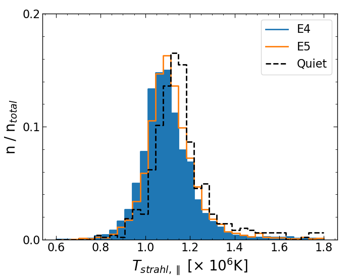
Figure 4: Distributions of the electron strahl temperatures during the E4 (blue), E5 (orange) and quiet (black) streams.

5 Conclusion

We have presented a comparison of two streams of slow Alfvénic wind measured at the same latitude and heliocentric distance by Parker Solar Probe (PSP) during its fourth and fifth solar encounters. From the statistically similar distributions of proton parameters (i.e. parallel and perpendicular temperatures, radial velocity, temperature anisotropy, density and $\beta_{\parallel}$) and electron strahl parallel temperature, we concluded that both wind streams had similar origins and were not associated with transient events.

We determined the source of this wind to be the boundary of the Southern polar coronal hole from PFSS modelling. The inertial range scaling of the power spectra and the high $\alpha$-proton drift velocities were consistent with coronal hole wind, and therefore were consistent with the solar source obtained from PFSS modelling. We explained with a flux tube argument from Kasper et al. (2007) that the low $\alpha$-particle abundance seen at 0.13 au could reasonably increase by a factor of $\sim 1.5$ to $\sim$ 0.9% at 1 au. This is consistent with previously measured $\alpha$-particle abundances in slow wind at 1 au (Alterman et al., 2021). The flux tube argument however, is not sufficient to explain the variability in $\alpha$-particle abundance seen in the solar wind at all heliocentric distances and more advanced models are needed.

We suggested that because the switchback statistics did not significantly change between the two streams measured 5 months and $\sim$ 30^∘ in surface longitude apart, the process leading to switchback formation does not display distinct temporal or spatial variation over these scales. Finally, as the two streams selected roughly corresponded to the spatial extent of switchback patches, we suggested that these patches are distinct features of coronal hole wind. The quiet periods that occur between patches could be related to spatial modulation in the solar source region or local transient events associated with the streamer belt. We proposed that, due to the similarity in the electron strahl temperature of the patches and the quiet period, that quiet periods could also be associated with coronal hole regions.

Future work could address how the $\alpha$-particle properties are linked to the solar source regions and characterise the ‘quiet’ intervals and patches. These studies will benefit from the decreasing PSP orbital distance and the constellation of spacecraft, including Solar Orbiter (Müller et al., 2013) and Bepi Colombo, now taking in-situ measurements in the heliosphere.

Streams

Stream	Start Time	End Time
E4 Stream	28 Jan 2020 12:07	28 Jan 2020 23:56
E5 Stream	06 Jun 2020 12:23	07 Jun 2020 00:21
Quiet Stream	28 Jan 2020 10:00	28 Jan 2020 12:00

Table 3: Start and end times for the E4, E5 and quiet streams.

Data Availability

The data used in this research is publicly available at: https://cdaweb.gsfc.nasa.gov/index.html/

Appendix A Potential Field Source Surface Mapping

References

- Abbo et al. (2016) Abbo L., et al., 2016, Space Sci. Rev., 201, 55
- Alterman et al. (2018) Alterman B. L., Kasper J. C., Stevens M. L., Koval A., 2018, ApJ, 864, 112
- Alterman et al. (2021) Alterman B. L., Kasper J. C., Leamon R. J., McIntosh S. W., 2021, Sol. Phys., 296, 67
- Altschuler & Newkirk (1969) Altschuler M. D., Newkirk G., 1969, Sol. Phys., 9, 131
- Badman et al. (2020) Badman S. T., et al., 2020, ApJS, 246, 23
- Bale et al. (2016) Bale S. D., et al., 2016, Space Sci. Rev., 204, 49
- Bale et al. (2019) Bale S. D., et al., 2019, Nature, 576, 237
- Bame et al. (1977) Bame S. J., Asbridge J. R., Feldman W. C., Gosling J. T., 1977, J. Geophys. Res., 82, 1487
- Berger et al. (2011) Berger L., Wimmer-Schweingruber R. F., Gloeckler G., 2011, Phys. Rev. Lett., 106, 151103
- Berčič et al. (2020) Berčič L., et al., 2020, ApJ, 892, 88
- Bourouaine & Chandran (2013) Bourouaine S., Chandran B. D. G., 2013, ApJ, 774, 96
- Breen et al. (2002) Breen A. R., Riley P., Lazarus A. J., Canals A., Fallows R. A., Linker J., Mikic Z., 2002, Annales Geophysicae, 20, 1291
- Burlaga & Ogilvie (1970) Burlaga L. F., Ogilvie K. W., 1970, ApJ, 159, 659
- Byhring (2011) Byhring H. S., 2011, ApJ, 738, 172
- Camporeale et al. (2017) Camporeale E., Carè A., Borovsky J. E., 2017, Journal of Geophysical Research (Space Physics), 122, 10,910
- Chandran (2010) Chandran B. D. G., 2010, ApJ, 720, 548
- Chen et al. (2020) Chen C. H. K., et al., 2020, ApJS, 246, 53
- Chen et al. (2021) Chen C. H. K., et al., 2021, A&A, (in press)
- Cranmer et al. (2007) Cranmer S. R., van Ballegooijen A. A., Edgar R. J., 2007, ApJS, 171, 520
- D’Amicis & Bruno (2015) D’Amicis R., Bruno R., 2015, ApJ, 805, 84
- D’Amicis et al. (2019) D’Amicis R., Matteini L., Bruno R., 2019, MNRAS, 483, 4665
- Dudok de Wit et al. (2020) Dudok de Wit T., et al., 2020, ApJS, 246, 39
- Einaudi et al. (1999) Einaudi G., Boncinelli P., Dahlburg R. B., Karpen J. T., 1999, J. Geophys. Res., 104, 521
- Feldman et al. (1978) Feldman W. C., Asbridge J. R., Bame S. J., Gosling J. T., 1978, J. Geophys. Res., 83, 2177
- Feldman et al. (1999) Feldman U., Widing K. G., Warren H. P., 1999, ApJ, 522, 1133
- Finley et al. (2020) Finley A. J., et al., 2020, A&A, (in press)
- Fisk (2003) Fisk L. A., 2003, Journal of Geophysical Research (Space Physics), 108, 1157
- Fisk & Schwadron (2001) Fisk L. A., Schwadron N. A., 2001, ApJ, 560, 425
- Fisk et al. (1999) Fisk L. A., Schwadron N. A., Zurbuchen T. H., 1999, J. Geophys. Res., 104, 19765
- Fox et al. (2016) Fox N. J., et al., 2016, Space Sci. Rev., 204, 7
- Fu et al. (2018) Fu H., Madjarska M. S., Li B., Xia L., Huang Z., 2018, MNRAS, 478, 1884
- Geiss et al. (1970) Geiss J., Hirt P., Leutwyler H., 1970, Sol. Phys., 12, 458
- Gloeckler et al. (2003) Gloeckler G., Zurbuchen T. H., Geiss J., 2003, Journal of Geophysical Research (Space Physics), 108, 1158
- Gosling et al. (1978) Gosling J. T., Asbridge J. R., Bame S. J., Feldman W. C., 1978, J. Geophys. Res., 83, 1401
- Harra et al. (2008) Harra L. K., Sakao T., Mandrini C. H., Hara H., Imada S., Young P. R., van Driel-Gesztelyi L., Baker D., 2008, ApJ, 676, L147
- Hellinger & Trávníček (2013) Hellinger P., Trávníček P. M., 2013, Journal of Geophysical Research (Space Physics), 118, 5421
- Hellinger et al. (2011) Hellinger P., Matteini L., Štverák Š., Trávníček P. M., Marsch E., 2011, Journal of Geophysical Research (Space Physics), 116, A09105
- Hirshberg et al. (1972a) Hirshberg J., Bame S. J., Robbins D. E., 1972a, Sol. Phys., 23, 467
- Hirshberg et al. (1972b) Hirshberg J., Asbridge J. R., Robbins D. E., 1972b, J. Geophys. Res., 77, 3583
- Horbury et al. (2018) Horbury T. S., Matteini L., Stansby D., 2018, MNRAS, 478, 1980
- Horbury et al. (2020) Horbury T. S., et al., 2020, ApJS, 246, 45
- Huang et al. (2020) Huang J., et al., 2020, arXiv e-prints, p. arXiv:2005.12372
- Jockers (1970) Jockers K., 1970, A&A, 6, 219
- Kasper et al. (2007) Kasper J. C., Stevens M. L., Lazarus A. J., Steinberg J. T., Ogilvie K. W., 2007, ApJ, 660, 901
- Kasper et al. (2012) Kasper J. C., Stevens M. L., Korreck K. E., Maruca B. A., Kiefer K. K., Schwadron N. A., Lepri S. T., 2012, ApJ, 745, 162
- Kasper et al. (2016) Kasper J. C., et al., 2016, Space Sci. Rev., 204, 131
- Kasper et al. (2019) Kasper J. C., et al., 2019, Nature, 576, 228
- Krieger et al. (1973) Krieger A. S., Timothy A. F., Roelof E. C., 1973, Sol. Phys., 29, 505
- Laker et al. (2020) Laker R., et al., 2020, A&A, (in press)
- Laker et al. (2021) Laker R., et al., 2021, arXiv e-prints, p. arXiv:2103.00230
- Laming (2004) Laming J. M., 2004, ApJ, 614, 1063
- Lavraud et al. (2020) Lavraud B., et al., 2020, ApJ, 894, L19
- Lemaire & Scherer (1970) Lemaire J., Scherer M., 1970, Planet. Space Sci., 18, 103
- Lemaire & Scherer (1971) Lemaire J., Scherer M., 1971, J. Geophys. Res., 76, 7479
- Li et al. (1999) Li X., Habbal S. R., Hollweg J. V., Esser R., 1999, J. Geophys. Res., 104, 2521
- Li et al. (2020) Li H., Wang C., Tu C., Xu F., 2020, Earth and Space Science, 7, e00997
- Lopez & Freeman (1986) Lopez R. E., Freeman J. W., 1986, J. Geophys. Res., 91, 1701
- Maksimovic et al. (1997) Maksimovic M., Pierrard V., Lemaire J. F., 1997, A&A, 324, 725
- Marsch et al. (1982a) Marsch E., Rosenbauer H., Schwenn R., Muehlhaeuser K. H., Neubauer F. M., 1982a, J. Geophys. Res., 87, 35
- Marsch et al. (1982b) Marsch E., Schwenn R., Rosenbauer H., Muehlhaeuser K. H., Pilipp W., Neubauer F. M., 1982b, J. Geophys. Res., 87, 52
- Maruca et al. (2012) Maruca B. A., Kasper J. C., Gary S. P., 2012, ApJ, 748, 137
- Matteini et al. (2012) Matteini L., Hellinger P., Landi S., Trávníček P. M., Velli M., 2012, Space Sci. Rev., 172, 373
- Matteini et al. (2014) Matteini L., Horbury T. S., Neugebauer M., Goldstein B. E., 2014, Geophys. Res. Lett., 41, 259
- Matteini et al. (2015a) Matteini L., Horbury T. S., Pantellini F., Velli M., Schwartz S. J., 2015a, ApJ, 802, 11
- Matteini et al. (2015b) Matteini L., Hellinger P., Schwartz S. J., Landi S., 2015b, ApJ, 812, 13
- Müller et al. (2013) Müller D., Marsden R. G., St. Cyr O. C., Gilbert H. R., 2013, Sol. Phys., 285, 25
- Neugebauer (1981) Neugebauer M., 1981, Fundamentals Cosmic Phys., 7, 131
- Neugebauer & Goldstein (2013) Neugebauer M., Goldstein B. E., 2013, in Zank G. P., et al., eds, American Institute of Physics Conference Series Vol. 1539, Solar Wind 13. pp 46–49, doi:10.1063/1.4810986
- Neugebauer et al. (1998) Neugebauer M., et al., 1998, J. Geophys. Res., 103, 14587
- Neugebauer et al. (2002) Neugebauer M., Liewer P. C., Smith E. J., Skoug R. M., Zurbuchen T. H., 2002, Journal of Geophysical Research (Space Physics), 107, 1488
- Nolte et al. (1976) Nolte J. T., et al., 1976, Sol. Phys., 46, 303
- O’Kane et al. (2021) O’Kane J., et al., 2021, A&A, (in press)
- Ogilvie & Wilkerson (1969) Ogilvie K. W., Wilkerson T. D., 1969, Sol. Phys., 8, 435
- Perrone et al. (2019) Perrone D., Stansby D., Horbury T. S., Matteini L., 2019, MNRAS, 488, 2380
- Perrone et al. (2020) Perrone D., D’Amicis R., De Marco R., Matteini L., Stansby D., Bruno R., Horbury T. S., 2020, A&A, 633, A166
- Rakowski & Laming (2012) Rakowski C. E., Laming J. M., 2012, ApJ, 754, 65
- Robbins et al. (1970) Robbins D. E., Hundhausen A. J., Bame S. J., 1970, J. Geophys. Res., 75, 1178
- Sanchez-Diaz et al. (2016) Sanchez-Diaz E., Rouillard A. P., Lavraud B., Segura K., Tao C., Pinto R., Sheeley N. R., Plotnikov I., 2016, Journal of Geophysical Research (Space Physics), 121, 2830
- Schatten et al. (1969) Schatten K. H., Wilcox J. M., Ness N. F., 1969, Sol. Phys., 6, 442
- Sheeley et al. (1976) Sheeley N. R. J., Harvey J. W., Feldman W. C., 1976, Sol. Phys., 49, 271
- Shoda et al. (2021) Shoda M., Chandran B. D. G., Cranmer S. R., 2021, arXiv e-prints, p. arXiv:2101.09529
- Smith et al. (2001) Smith C. W., Matthaeus W. H., Zank G. P., Ness N. F., Oughton S., Richardson J. D., 2001, J. Geophys. Res., 106, 8253
- Squire et al. (2020) Squire J., Chandran B. D. G., Meyrand R., 2020, ApJ, 891, L2
- Stansby et al. (2018) Stansby D., Salem C., Matteini L., Horbury T., 2018, Sol. Phys., 293, 155
- Stansby et al. (2019a) Stansby D., Horbury T. S., Matteini L., 2019a, MNRAS, 482, 1706
- Stansby et al. (2019b) Stansby D., Perrone D., Matteini L., Horbury T. S., Salem C. S., 2019b, A&A, 623, L2
- Stansby et al. (2020a) Stansby D., Yeates A., Badman S. T., 2020a, Journal of Open Source Software, 5, 2732
- Stansby et al. (2020b) Stansby D., Matteini L., Horbury T. S., Perrone D., D’Amicis R., Berčič L., 2020b, MNRAS, 492, 39
- Sterling & Moore (2020) Sterling A. C., Moore R. L., 2020, ApJ, 896, L18
- Tu et al. (2005) Tu C.-Y., Zhou C., Marsch E., Xia L.-D., Zhao L., Wang J.-X., Wilhelm K., 2005, Science, 308, 519
- Verdini et al. (2010) Verdini A., Velli M., Matthaeus W. H., Oughton S., Dmitruk P., 2010, ApJ, 708, L116
- Verniero et al. (2020) Verniero J. L., et al., 2020, ApJS, 248, 5
- Verscharen et al. (2015) Verscharen D., Chandran B. D. G., Bourouaine S., Hollweg J. V., 2015, ApJ, 806, 157
- Verscharen et al. (2019) Verscharen D., Klein K. G., Maruca B. A., 2019, Living Reviews in Solar Physics, 16, 5
- Viall & Borovsky (2020) Viall N. M., Borovsky J. E., 2020, Journal of Geophysical Research (Space Physics), 125, e26005
- Wang & Sheeley (1994) Wang Y. M., Sheeley N. R. J., 1994, J. Geophys. Res., 99, 6597
- Whittlesey et al. (2020) Whittlesey P. L., et al., 2020, ApJS, 246, 74
- Woodham et al. (2020) Woodham L. D., et al., 2020, A&A, (in press)
- Woolley et al. (2020) Woolley T., et al., 2020, MNRAS, 498, 5524
- Xu & Borovsky (2015) Xu F., Borovsky J. E., 2015, Journal of Geophysical Research (Space Physics), 120, 70
- Zank et al. (2020) Zank G. P., Nakanotani M., Zhao L. L., Adhikari L., Kasper J., 2020, ApJ, 903, 1