Progress on the calibration of surface brightness–color relations for early- and late-type stars

Abstract

Context. Surface brightness-color relations (SBCRs) are widely used for estimating angular diameters and deriving stellar properties. They are critical to derive extragalactic distances of early-type and late-type eclipsing binaries or, potentially, for extracting planetary parameters of late-type stars hosting planets. Various SBCRs have been implemented so far, but strong discrepancies in terms of precision and accuracy still exist in the literature.

Aims. We aim to develop a precise SBCR for early-type B and A stars using selection criteria, based on stellar characteristics, and combined with homogeneous interferometric angular diameter measurements. We also improve SBCRs for late-type stars, in particular in the Gaia photometric band.

Methods. We observed 18 early-type stars with the VEGA interferometric instrument, installed on the CHARA array. We then applied additional criteria on the photometric measurements, together with stellar characteristics diagnostics in order to build the SBCRs.

Results. We calibrated a SBCR for subgiant and dwarf early-type stars. The RMS of the relation is $\sigma_{F_{V_{0}}}=0.0051\,$mag, leading to an average precision of 2.3% on the estimation of angular diameters, with 3.1% for $V-K<-0.2\,$mag and 1.8% for $V-K>-0.2\,$mag. We found that the conversion between Johnson-$K$ and 2MASS-$K_{s}$ photometries is a key issue for early-type stars. Following this result, we have revisited our previous SBCRs for late-type stars by calibrating them with either converted Johnson-$K$ or 2MASS-$K_{s}$ photometries. We also improve the calibration of these SBCRs based on the Gaia photometry. The expected precision on the angular diameter using our SBCRs for late-type stars ranges from 1.0% to 2.7%.

Conclusions. By reaching a precision of 2.3% on the estimation of angular diameters for early-type stars, significant progress has been made to determine extragalactic distances, such as M31 and M33 galaxies, using early-type eclipsing binaries.

1 Introduction

Determining the expansion of the Universe, that is the Hubble constant ($H_{0}$) to better than 2%, is required in order to understand the nature of dark energy. However, the two most accurate methods for that, the cosmic microwave background (Planck Collaboration et al., 2020; Riess et al., 2019) and the distance ladder, are inconsistent today, which is referred to as the ”tension” (Wong et al., 2020). One of the keys to resolve this tension is based on the calibration of the Leavitt period-luminosity (PL) law of Cepheids (Leavitt & Pickering, 1912). Cepheids are indeed the backbone of the extragalactic distance ladder because their pulsation periods, which are easily determined observationally, directly correlate with their luminosities. Another method consists in using eclipsing binaries to constrain extragalactic distances.

Recently, a new estimate of the distance to the Large Magellanic Cloud (LMC), based on 20 late-type eclipsing binaries, has been obtained by the Araucaria team (Pietrzyński et al., 2019). Their precision of 1% is mostly due to the precision of the surface brightness-color relation (SBCR), calibrated on 41 nearby red clump giant stars using infrared interferometry (Gallenne et al., 2018). The same was done to derive the distance of the Small Magellanic Cloud (SMC) with a precision of better than 2% (Graczyk et al., 2020). Deriving the distance from eclipsing binaries is simple: the radius of both components is estimated from the combination of photometry and spectroscopy, and angular diameters are estimated from the magnitude and color of stars through a SBCR. The combination of radii and angular diameters provides the distance. The influence of interstellar attenuation in neighboring galaxies has been studied using several techniques so far (Bonanos et al., 2006; Pietrzyński et al., 2019; Graczyk et al., 2020), and it is still under investigation.

The situation concerning the early-type eclipsing binaries is more complex because the calibration of the SBCR requires high angular resolution measurements, and early-type stars are particularly active (Martins et al., 2015; Gordon et al., 2018). Challouf et al. (2014) improved, by a factor of 2, the precision on SBCR of early-type stars from about 15% to 7%, corresponding to the most accurate SBCR developed so far for early-type stars. However, this precision is still not sufficient to derive the distance of extragalactic early-type eclipsing binaries with a precision of a few percent. It is also worthwhile to mention that the distances to M31 and M33 are currently based on models of early-type eclipsing binaries, but not SBCRs (Bonanos et al., 2006; Vilardell et al., 2010). Another interesting approach is to analyze O- and B-type detached eclipsing binaries in the LMC, for which the distance is known, and to derive the surface brightness (Taormina et al., 2019). In this paper, we aim to calibrate the SBCR for early-type stars precisely, following the strategy of Paper I.

Moreover, with the work done on the infrared photometry of early-type stars, it is now possible to improve the SBCRs for late-type stars shown in Salsi et al. (2020) (Paper I hereafter). It turns out that some refinements are necessary concerning the infrared photometric systems that are used. Finally we have also reconsidered the calculation of the extinction in the Gaia band for proposing a new improvement of the SBCRs in this work.

Sect. 2, 3, 4 are devoted to the strategy and data selection, the VEGA observations, and the SBCR calibration of early-type stars, respectively. A subsequent discussion is provided in Sect. 5. The revision of SBCR for late-type stars is presented in Sect. 6, while some general conclusions are given in Sect. 7.

2 Strategy and data selection

2.1 Criteria on stellar characteristics

In Paper I, we have shown that any stellar activity or characteristics (multiplicity, binarity, variability, etc.) may impact the calibration of SBCRs. We therefore implemented a set of criteria to select a correct sample of early-type stars.

We restricted the calibration of our SBCR to $V$ and $K$ photometries, as it is the set of color which provides the lowest dispersion (Kervella et al., 2004). We started the selection from the SIMBAD Astronomical Database. We first selected early-type stars, thus O, B, and A stars with $V-K<1\,$mag. We then considered only subgiants and dwarfs. From Challouf et al. (2015), we know that the projected rotational velocity affects the surface brightness of the star. They show that a rotational velocity lower than 85% of the critical velocity has an impact of at most $\sigma_{F_{V}}=$ 0.003 mag on the RMS of the SBCR. Alternatively, if one cannot access the critical velocity of the star, they demonstrate that considering stars with projected rotational velocity $V_{\mathrm{rot}}\sin i$ lower than $100$ km/s also results in a dispersion of 0.003 mag. Therefore, to reach a precision of $\sim$2% on the angular diameter estimate, we made the choice to consider only stars with $V_{\mathrm{rot}}\sin i$ lower than 75 km/s.

We excluded all known binary stars in our sample. The SEDs of all the stars were checked with the VO Sed Analyzer (VOSA) software.

We have shown in Paper I that a variability above 0.1 mag could significantly affect the SBCR. Following this strategy, we searched for information about the variability of the stars in Samus’ et al. (2017). We then rejected variable stars with a variability above 0.1 mag. We quantitatively study this point later in Sect. 5.1.

We finally searched for stars with expected angular diameters between 0.3 and 0.8 milli-second of arc (mas). This is optimal for the VEGA instrument (Mourard et al., 2009, 2011), installed at the CHARA array in Mount Wilson, USA (ten Brummelaar et al., 2005). We finally end up with a total of 18 stars to be observed in the northern hemisphere. No O-type stars were selected due to a roughly equal combination of variability and multiplicity criteria.

2.2 Photometric selection and interstellar attenuation

As demonstrated in Paper I, precise photometries are of course mandatory for the calibration of SBCR. The Kharchenko & Roeser (2009) catalog offers precise visible magnitudes and gathers measurements from several other catalogs (Hipparcos-Tycho catalogs, Carlsberg Meridian Catalog, and the Positions and Proper Motions catalog). All the visible magnitudes are given in the Johnson-$V$ filter. With such a catalog, the precision on the $V$ magnitude of our stars ranges from 0.002 mag to 0.008 mag.

Finding precise infrared $K$ photometry is more complex. Indeed, we faced some issues with the 2MASS catalog (Cutri et al., 2003), where seven out of the 18 stars in our sample are affected by imprecise infrared measurements (i.e., an uncertainty higher than 0.1 mag). This problem has already been identified in Paper I and is due to saturation issues. We identified accurate measurements in Ducati (2002) for these seven stars.

The precision on the $K/K_{s}$ photometry in our sample ranges from 0.1% to 2.7%. However, the drawback of this approach is that the selected photometric values are inhomogeneous in terms of the filter pass band. We could convert Johnson-$K$ photometries into 2MASS using transformation equations, as we propose later in Sect. 6 for late-type stars, but this leads to other issues, in particular for early-type stars, that are discussed in Sect. 5.2.

For the reddening correction, we used the Stilism online tool (Lallement et al., 2014; Capitanio et al., 2017) to compute the color excess $E(B-V)$, considering early Gaia DR3 parallaxes (Gaia Collaboration et al., 2021, 2018). The interest of this tool is the tridimensional maps of the local interstellar matter (ISM) it offers, based on measurements of starlight absorption by dust or gaseous species. The interstellar attenuation $A_{V}$ in the visible band is defined as follows

$$A_{V}=R_{V}\times E(B-V),$$ (1)

where $R_{V}$ is the total-to-selective extinction ratio in the visible band, for which we set $R_{V}=3.1$, and we used $A_{K}=0.114\times A_{V}$ (Cardelli et al., 1989).

3 VEGA/CHARA interferometric measurements

Table 1: Reference stars used for VEGA observations listed with their spectral type, their $V$ magnitude, and their uniform-disk angular diameter in the $R$ band. Sect. 3 describes the parameters of the calibrators.

Target	Reference	Sp. Type	$V$	$\theta_{\mathrm{UD}}$[R]
	stars		[mag]	[mas]
HD11415	HD10221	A0V	5.59	$0.224_{\pm 0.013}$
	HD12301	A0I	5.61	$0.403_{\pm 0.013}$
	HD6210	F6V	5.83	$0.489_{\pm 0.039}$
HD114330	HD107070	A5IV/V	5.90	$0.289_{\pm 0.021}$
	HD112846	A3III	5.79	$0.294_{\pm 0.009}$
	HD116831	A8V	5.97	$0.279_{\pm 0.019}$
HD145389	HD140728	A0V	5.48	$0.232_{\pm 0.015}$
	HD143584	F0IV	6.03	$0.327_{\pm 0.023}$
	HD144206	B9III	4.71	$0.314_{\pm 0.019}$
HD145570	HD143459	A0V	5.53	$0.272_{\pm 0.019}$
	HD145607	A2IV	5.42	$0.307_{\pm 0.023}$
HD148112	HD144874	A7V	5.64	$0.340_{\pm 0.024}$
	HD152614	B8V	4.38	$0.333_{\pm 0.024}$
HD149438	HD146624	A1V	4.78	$0.339_{\pm 0.023}$
	HD148605	B3V	4.79	$0.213_{\pm 0.015}$
HD152107	HD143584	F0IV	6.03	$0.327_{\pm 0.023}$
	HD144206	B9III	4.71	$0.314_{\pm 0.019}$
	HD149303	A2V	5.68	$0.286_{\pm 0.020}$
	HD155860	A5III	6.13	$0.231_{\pm 0.017}$
HD192640	HD191610	B2.5V	4.93	$0.210_{\pm 0.018}$
	HD193369	A2V	5.58	$0.263_{\pm 0.016}$
HD195810	HD193472	A5	5.94	$0.319_{\pm 0.023}$
	HD196544	A1IV	5.42	$0.270_{\pm 0.008}$
	HD196740	B5IV	5.05	$0.210_{\pm 0.012}$
HD27819	HD25202	F4V	5.87	$0.376_{\pm 0.026}$
	HD28226	Am	5.71	$0.345_{\pm 0.025}$
HD27962	HD27459	F0IV/V	5.24	$0.409_{\pm 0.029}$
	HD28226	Am	5.71	$0.345_{\pm 0.025}$
HD3360	HD1976	B5IV	5.58	$0.200_{\pm 0.006}$
	HD2054	B9IV	5.72	$0.207_{\pm 0.006}$
	HD3240	B7III	5.08	$0.238_{\pm 0.015}$
	HD6676	B8V	5.77	$0.207_{\pm 0.014}$
HD33959	HD34452	A0	5.37	$0.214_{\pm 0.006}$
	HD34578	A5II	5.03	$0.597_{\pm 0.055}$
	HD35239	B9III	5.93	$0.227_{\pm 0.016}$
	HD35520	A1p	5.91	$0.301_{\pm 0.008}$
HD35468	HD34203	A0V	5.52	$0.251_{\pm 0.016}$
	HD34658	F3III/IV	5.32	$0.498_{\pm 0.038}$
	HD37490	B3V	4.59	$0.229_{\pm 0.023}$
	HD38899	B9IV	4.88	$0.298_{\pm 0.019}$
HD58142	HD47100	B8III	5.33	$0.236_{\pm 0.014}$
	HD56963	F2V	5.74	$0.405_{\pm 0.030}$
	HD60652	A5m	5.91	$0.283_{\pm 0.019}$
	HD70313	A3V	5.54	$0.300_{\pm 0.020}$
HD886	HD1439	A0IV	5.88	$0.207_{\pm 0.013}$
	HD560	B9V	5.53	$0.219_{\pm 0.013}$
HD89021	HD85795	A3III	5.27	$0.297_{\pm 0.021}$
	HD90470	A3V	6.01	$0.264_{\pm 0.007}$
	HD90840	A4V	5.78	$0.276_{\pm 0.018}$
	HD91312	A7IV	4.72	$0.554_{\pm 0.036}$
	HD94334	A1V	4.66	$0.368_{\pm 0.011}$
HD97633	HD92825	A3V	5.07	$0.346_{\pm 0.022}$
	HD93702	A2V	5.31	$0.301_{\pm 0.022}$
	HD95608	A1V	4.40	$0.453_{\pm 0.036}$

Table 2: VEGA angular diameter measurements for the 18 early-type stars (see Sect. 3 for a detailed description of the method used to derive the angular diameter of stars).

Name	Sp.Type	$V$	$A_{V}$	$(V-K)_{0}$	$K$-ref	$u_{\mathrm{R}}$	$\theta_{\mathrm{LD}_{\pm\sigma_{\theta_{\mathrm{LD}}}}}$	$\chi^{2}_{r}$
		[mag]	[mag]	[mag]			[mas]
HD11415	B2V	3.35	0.050	$-0.484_{\pm 0.012}$	Ducati (2002)	0.281	$0.471_{\pm 0.007}$	1.097
HD114330	A1IV	4.38	0.012	$-0.022_{\pm 0.04}$	Cutri et al. (2003)	0.413	$0.443_{\pm 0.023}$	1.107
HD145389	B9V	4.23*	0.028	$-0.115_{\pm 0.017}$	Cutri et al. (2003)	0.358	$0.452_{\pm 0.007}$	0.089
HD145570	A1V	4.93	0.003	$0.297_{\pm 0.02}$	Cutri et al. (2003)	0.512	$0.431_{\pm 0.008}$	0.114
HD148112	A2V	4.57*	0.016	$0.036_{\pm 0.022}$	Ducati (2002)	0.410	$0.423_{\pm 0.010}$	0.089
HD149438	B0V	2.82	0.214	$-0.939_{\pm 0.032}$	Ducati (2002)	0.235	$0.338_{\pm 0.011}$	0.528
HD152107	A1V	4.82*	0.022	$0.229_{\pm 0.022}$	Cutri et al. (2003)	0.434	$0.432_{\pm 0.009}$	0.134
HD192640	A2V	4.95*	0.009	$0.520_{\pm 0.02}$	Cutri et al. (2003)	0.447	$0.489_{\pm 0.011}$	0.244
HD195810	B6IV	4.03*	0.053	$-0.398_{\pm 0.038}$	Cutri et al. (2003)	0.319	$0.394_{\pm 0.003}$	0.038
HD27819	A2V	4.80	0.003	$0.347_{\pm 0.014}$	Ducati (2002)	0.468	$0.489_{\pm 0.007}$	1.592
HD27962	A2IV	4.30*	0.003	$0.199_{\pm 0.033}$	Cutri et al. (2003)	0.350	$0.538_{\pm 0.013}$	0.587
HD3360	B2IV	3.67*	0.090	$-0.618_{\pm 0.038}$	Cutri et al. (2003)	0.278	$0.350_{\pm 0.004}$	0.299
HD33959	A9V	5.00*	0.006	$0.610_{\pm 0.026}$	Cutri et al. (2003)	0.476	$0.515_{\pm 0.004}$	0.472
HD35468	B2V	1.64*	0.003	$-0.686_{\pm 0.038}$	Ducati (2002)	0.267	$0.785_{\pm 0.007}$	1.162
HD58142	A0.5V	4.61	0.006	$0.033_{\pm 0.018}$	Cutri et al. (2003)	0.410	$0.419_{\pm 0.008}$	0.303
HD886	B2IV	2.83*	0.034	$-0.756_{\pm 0.032}$	Ducati (2002)	0.277	$0.435_{\pm 0.004}$	0.478
HD89021	A1IV	3.43	0.006	$0.045_{\pm 0.094}$	Ducati (2002)	0.453	$0.757_{\pm 0.007}$	0.389
HD97633	A2IV	3.32	0.003	$0.017_{\pm 0.094}$	Cutri et al. (2003)	0.431	$0.769_{\pm 0.010}$	1.443

We observed the sample of 18 early-type stars from 23 February 2019 to 16 December 2020. The calibrated oifits files are available on OIdB. The data were processed using the standard VEGA pipeline (Mourard et al., 2009) and the squared visibilities were calibrated using reference stars selected with the SearchCal tool (Bonneau et al., 2006). The list of the calibrators is included in Table 1. The uniform-disk angular diameter in the $R$ band $\theta_{\mathrm{UD}}$[R] is taken from the JMMC Stellar Diameters Catalogue version 2 (Bourges et al., 2017, JSDC2), but we consider the uncertainties from the JDSC version 1 (Lafrasse et al., 2010), which is more conservative. The observing log is given in Table LABEL:observing_table. The systematic uncertainties stem from the uncertainties on the calibrator diameters, given in Table 1, and they are negligible with respect to the statistical ones.

We used the JMMC LitPro tool (Tallon-Bosc et al., 2008) to fit a model of a linear limb-darkened disk on the calibrated squared visibilities. This model has the following two parameters: the limb-darkened angular diameter and the limb-darkening coefficient, $u_{R}$. Considering the precision of the VEGA measurements and the range of spatial frequencies that have been covered, we cannot adjust the coefficient of the limb darkening. The $u_{R}$ coefficient for each star is fixed and taken from the Claret & Bloemen (2011) catalog. We searched for the effective temperature $T_{\mathrm{eff}}$, the gravity $\log g$, and the metallicity $Z$ of the star and we took the closest value of each parameter available in the catalog in order to determine $u_{R}$. Claret’s grids have a step of 250 K in temperature, thus the largest error we can make on the temperature is 125 K without any interpolation. This error on the temperature leads to an average error of 0.05% on the angular diameter, which is well below our typical errors.

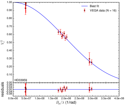
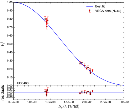
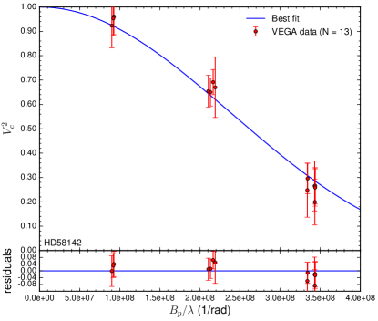
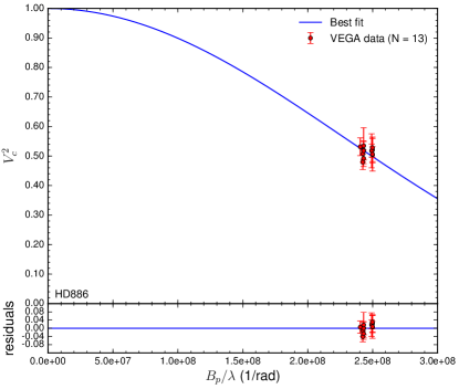
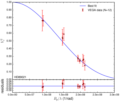
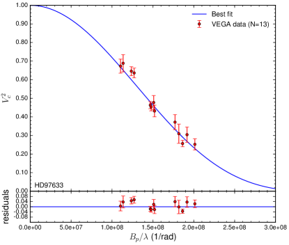
Figure 6: Squared visibility versus spatial frequency for all stars in our sample with their corresponding statistical uncertainties (red dots). The solid blue lines indicate the best uniform-disk model obtained from the LITpro fitting software. See Sect. 3 for a detailed description of the fitting strategy.

This parameter is fixed in the fitting process of the LITpro tool. The coefficient $u_{R}$ is given in Table 2 together with the derived limb-darkened angular diameter. The corresponding visibility curves are presented in Fig. 6. The precision on the angular diameter that we obtain ranges from 0.78% to 5.10%, with a median value of 1.8%.

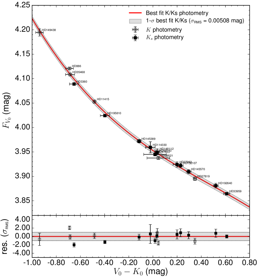
Figure 1: $F_{V_{0}}$ derived in this work as a function of $(V-K)_{0}$. Empty squares are data with a $K$ Johnson photometry, while filled squares are those with a $K_{s}$ photometry. The third-order SBCR for early-type dwarfs is shown by the red solid line. The gray area denotes the RMS of the relation. The bottom panel presents the residual in units of the RMS of the relation. See Sect. 4 for a description of the fitting strategy.

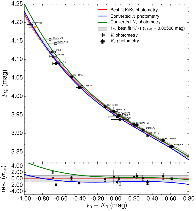
Figure 2: Comparison between our SBCR with mixed Johnson-2MASS photometries (red solid line), SBCR with converted 2MASS $K_{s}$ photometry (green solid line), and Johnson-$K$ photometry (blue solid line) for early-type stars. Light-gray dots are eclipsing binaries from Taormina et al. (2019). The orange dot shows the data for HD149438 using the Hipparcos parallax. See Sect. 5.2 for detailed information on the converted SBCRs.

4 Calibration of the SBCR for early-type stars

The surface brightness $S_{\lambda}$ of a star is correlated to its limb-darkened angular diameter $\theta_{\mathrm{LD}}$ and its apparent magnitude corrected from the extinction $m_{\lambda_{0}}$ by the following formula (Wesselink, 1969)

$$S_{\lambda}=m_{\lambda_{0}}+5\log\theta_{\mathrm{LD}}.$$ (2)

Wesselink (1969) used this definition to highlight the correlation between the surface brightness and the color of the star by the relation below:

$$S_{\lambda_{1}}=\sum_{n=0}^{N}C_{n}(m_{\lambda_{1}}-m_{\lambda_{2}})_{0}^{n},$$ (3)

which defines the so-called SBCR. Later, Barnes & Evans (1976) developed another definition of the SBCR, which we denote as $F_{\lambda}$. To be consistent with the strategy of Paper I, we consider the Barnes & Evans (1976) definition in the rest of our study, namely

$$F_{\lambda_{1}}=4.2196-0.1\times\left\{\sum_{n=0}^{N}C_{n}(m_{\lambda_{1}}-m_{\lambda_{2}})_{0}^{n}\right\}.$$ (4)

The 18-star sample covers a range of $V-K$ color from -1 to +0.6 mag. We computed the surface brightness of the 18 stars following Eq. 4. Our fitting strategy uses the orthogonal distance regression (ODR), which considers both $F_{V}$ and $V-K$ errors. A more detailed description can be found in Appendix A of Paper I. The final SBCR for early-type stars combining Johnson and 2MASS photometries ($K$/$K_{s}$ SBCR hereafter) is then shown in Fig. 1. The coefficients of our SBCR are shown in the first row of Table 3, together with their uncertainties. We discuss the possibility of converting all the photometric measurements into the same system in Sect. 5.2. We restricted our SBCR to the third order.

Table 3: Parameters of $K/K_{s}$ and converted SBCRs for early-type stars (see Sect. 5.2 for a description of the conversions).

	$N_{c}$ /$N$	$C_{0}$	$C_{1}$	$C_{2}$	$C_{3}$	$\sigma_{\mathrm{RMS}}$	Expected $\frac{\sigma{\theta_{\mathrm{LD}}}}{\theta_{\mathrm{LD}}}$
						[mag]	[%]
$K/K_{s}$		$2.6675_{\pm 0.0149}$	$1.6556_{\pm 0.0571}$	$-0.6084_{\pm 0.0667}$	$0.4350_{\pm 0.1530}$	0.00508	2.34
$K$	11/18	$2.7162_{\pm 0.0196}$	$1.6267_{\pm 0.0773}$	$-0.6191_{\pm 0.1011}$	$0.5733_{\pm 0.2276}$	0.00770	3.55
$K_{s}$	7/18	$2.6434_{\pm 0.0199}$	$1.6845_{\pm 0.0792}$	$-0.6947_{\pm 0.0924}$	$0.5734_{\pm 0.2276}$	0.00770	3.55

Using Eq. 2 with visible $V$ magnitudes, we have:

$$\theta_{\mathrm{LD}}=10^{8.4392-0.2V_{0}-2F_{V_{0}}}.$$ (5)

Applying the partial derivative method on Eq. 5 gives

$$\frac{\sigma_{\theta_{\mathrm{LD}_{\mathrm{rms}}}}}{\theta_{\mathrm{LD}}}=2\ln(10)\sigma_{F_{V_{0}}}.$$ (6)

The average RMS of the relation is found to be $\sigma_{F_{V_{0}}}=0.00508\,$mag. This corresponds to a relative precision on the angular diameter of 2.3%, according to Eq. 6. However, the lack of measurements in the blue part (i.e., $V-K<-0.2\,$mag) has to be taken into account. We split the $V-K$ validity domain into two ranges, namely $-0.8\,$mag $<V-K<-0.2\,$mag and $-0.2\,$mag $<V-K<0.6\,$mag, and we computed the RMS of the SBCR on both ranges. For $V-K<-0.2\,$mag, we expect a precision of 3.1% on the angular diameter. On the other hand, the expected precision is 1.8% for $V-K>-0.2\,$mag.

5 Discussion

5.1 Impact of the variability on the SBCR

As in Paper I, we aimed to quantify the impact of the variability on the SBCR. In our sample of early-type stars, ten out of 18 stars are flagged as variables. Their variability ranges from $\pm 0.01\,$mag to $\pm 0.06\,$mag according to Samus’ et al. (2017), with a median value at 0.04 mag. We computed a SBCR considering an offset on the $V$ magnitude of the ten variable stars corresponding to their maximum amplitude. The resulting SBCR is consistent at a level of less than 1$\sigma$ with the current SBCR all over the $V-K$ validity domain. We conclude that a variability under 0.06 mag does not have any consequence on our result. Keeping these variable stars in the sample is therefore acceptable.

5.2 The $K$-band photometry of early-type stars

The Johnson-$K$ and 2MASS-$K_{s}$ photometries of our sample are not equally distributed in terms of V-K colors (see Fig. 1), which prevents one from calibrating a purely homogeneous SBCR, which is either based on $K$ or $K_{s}$, respectively. We therefore made the choice of combining $K$ and $K_{s}$ data to calibrate the SBCR. The precision we expect on the angular diameter using this relation is 2.3%, but we do not exclude a bias due to the fact that we mixed different infrared photometric bands. However, using the conversion relations $K$ to $K_{s}$ or the reverse also implies some difficulties. Indeed, the typical transformation equations (Bessell & Brett, 1988; Carpenter, 2001) are indirectly deduced from the 2MASS-CIT and 2MASS-SAAO equations of Bessell & Brett (1988) and Carpenter (2001). Moreover, the CIT equation of Bessell & Brett (1988) is based on the observation of only 21 stars, and the bluer spectral type of the sample is B7. Regarding our sample, this corresponds to a V-K color of $-0.3\,$mag. Nevertheless, the resulting converted SBCRs are shown as blue and green solid lines in Fig. 2 for Johnson-$K$ and 2MASS-$K_{s}$ photometries respectively. The coefficients are shown in Table 3. The converted Johnson-$K$ SBCR is consistent with the inhomogeneous SBCR at less than $1\sigma$ over all the $V-K$ validity domain. Concerning the uniform 2MASS relation, such a conversion does not influence the calibration of the SBCR at more than 1$\sigma$ for V-K ¿ -0.4  mag. The inconsistency, however, reaches more than 4$\sigma$ for the bluest part of the relation. The expected precision on the angular diameter using a SBCR based on a uniform set of photometry is of 3.6%.

In conclusion, if one wants to derive the angular diameter of a star with $K$ photometry, we suggest using the $K$/$K_{s}$ or $K$ SBCRs in Table 3, with a good level of confidence, the $K$/$K_{s}$ relation being the most precise. If instead one has $K_{s}$ photometry for his or her star, using the SBCR based on $K_{s}$ is more consistent, but a bias due to the conversion from $K$ to $K_{s}$ in the calibration process of the SBCR is not excluded, as already discussed. Future investigations are needed to evaluate the consistency of such photometric conversion relations on the early-type stars’ color range.

5.3 Comparison with the literature

HD35468 was already observed by Challouf et al. (2014) and they obtained an angular diameter of 0.715 $\pm$ 0.005 mas, whereas our measurement is 0.786 $\pm$ 0.007 mas. Challouf et al. (2014) took the uniform-disk angular diameter of their calibrators in the JSDC (Lafrasse et al., 2010), while we used the second version of the catalog (Bourges et al., 2017). We processed the measurements of Challouf et al. (2014) using the JSDC2 angular diameters measurements for the three calibrators of Challouf et al. (2014), and with the same strategy described in this work. We found an angular diameter of 0.807 $\pm$ 0.026 mas, which is consistent with our value at a level of 1$\sigma$. This clearly shows some bias in the initial data reduction of Challouf et al. (2014) due to differences between JSDC and JSDC2 angular diameters.

In addition to HD35468, two other stars in Table 2 have been observed previously at CHARA. For HD97633, Maestro et al. (2013) measured an angular diameter of 0.740 $\pm$ 0.024 mas using PAVO, which is consistent with our result. The PAVO measurements of both Maestro et al. (2013) and Gordon et al. (2019) led to a smaller value for the angular diameter for HD3360 (0.311 $\pm$ 0.010 mas and 0.280 $\pm$ 0.018 mas, respectively). The diameter measurements in both papers are based on only two observations, so they could be more susceptible to systematic errors. Also, Casagrande et al. (2014) and White et al. (2018) found increased discrepancies as the angular diameters approached the resolution limits, which is the case here with such a value for the angular diameter for HD3360.

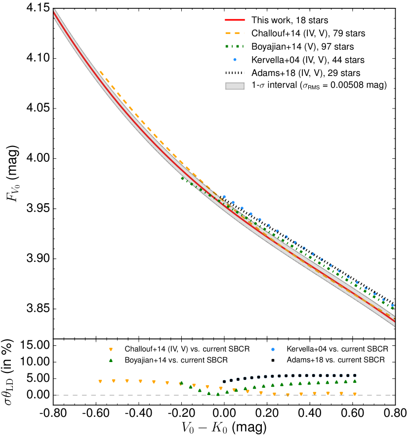
Figure 3: Top panel: Comparison between our SBCR for early-type stars and relations of Challouf et al. (2014), Boyajian et al. (2014), Kervella et al. (2004), and Adams et al. (2018). Bottom panel: Differences in angular diameter estimates between our SBCR and the other relations. See Sect. 5.3 for more details on the comparison.

We also compared our extinction values with those of Challouf et al. (2014). We computed the extinction of our 18 stars by combining the $Q$-method from Johnson & Morgan (1953) and the intrinsic colors method by Wegner (2014). We found consistent results with Stilism, except for one star, namely HD149438. This star has a smaller Gaia parallax value than Hipparcos, but the values of the extinction are consistent ($A_{v}=0.21\,$mag for Gaia versus $A_{V}=0.15\,$mag for Hipparcos). The uncertainty of the Gaia parallax is larger than the one of Hipparcos. We suggest this star could be oversaturated in Gaia photometry broadbands. In Fig. 2, we included the data for HD149438 using the Hipparcos parallax (orange dot). The choice of the parallax does not affect the SBCR at more than 1$\sigma$. For consistency, we decided to keep the Gaia parallax value for HD149438 in this work.

In Fig. 3, we included a comparison between our SBCR for early-type stars and the relations of Boyajian et al. (2014), Kervella et al. (2004), Challouf et al. (2014), and Adams et al. (2018). The bottom panel shows the normalized difference we expect in terms of the angular diameter between our SBCR and these relations on the $-0.6<V-K<$ 0.6 mag color range. The first two references have been largely used so far, and their $V-K$ color domain of validity cover a large part of the early-type range. Conversely to our SBCR, these relations are fully linear. We expect a difference on the angular diameter of more than 5% for $V-K>0\,$mag using the relations of Kervella et al. (2004) and Adams et al. (2018). We find an agreement of less than 4% on the angular diameter with the linear relation of Boyajian et al. (2014) for $V-K>-0.2\,$mag. This comparison demonstrates that a linear SBCR for early-type stars is no longer valid for $V-K<-0.2\,$mag. Comparing our new relation with the dwarfs relation of Challouf et al. (2014) leads to a good agreement of less than 5% on -0.6 $<V-K<0.6\,$mag. The agreement is even more evident for $V-K>0\,$mag, with a difference of at most 2% on the angular diameter estimate.

Among the eight stars measured by Challouf et al. (2014), six of them do not fulfill the stellar characteristics criteria, which can also explain this gap. The inconsistency we see for $V-K<-0.2\,$mag can also be explained by the consideration of photometric uncertainties. Indeed, Challouf et al. (2014) have assumed respective errors of 0.015 mag and 0.03 mag on the $V$ and $K$ photometries of their sample, while, via this work, we see that the infrared $K$ photometry plays a major role in the calibration of a SBCR. The uncertainty on the $K$ photometry often exceeds 0.03 mag in our sample, considering an arbitrary error could therefore induce an underestimation of the photometric uncertainty and finally a bias in the calibration of the relation.

Taormina et al. (2019, 2020) analyzed two early-type eclipsing binaries in the LMC with the aim to obtain precise and accurate stellar parameters of each early-type stars, which were then used to derive the surface brightness. They compare the measurements of their first binary system BLMC-01 of class IV or V, with the all-classes relation of Challouf et al. (2014) and they find good agreement. However, their measurements are inconsistent with our inhomogeneous $K/K_{s}$ SBCR (see light-gray dots on Fig. 2) at more than 5.5$\sigma$. The disagreement is lower but still significant when considering the SBCR converted into $K_{s}$ system. Such inconsistencies require more investigation.

6 Updating late-type stars SBCRs and linking to early-type stars

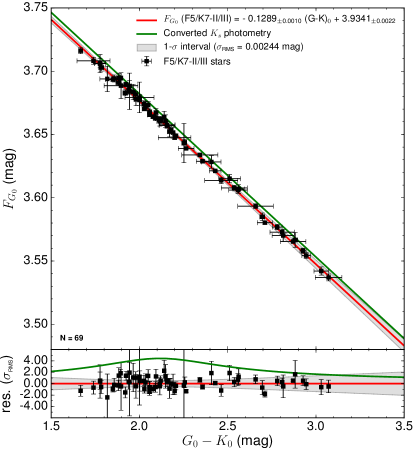
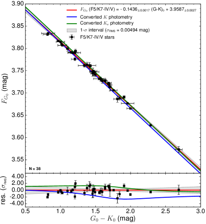
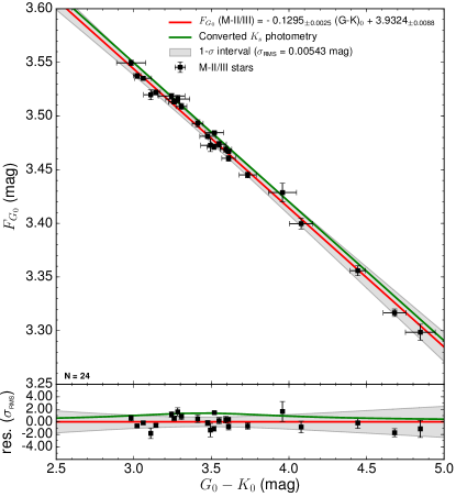
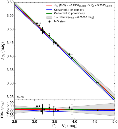
Figure 4: Converted SBCRs for late-type stars using Gaia photometry, plotted above the data (black squares). Relations with converted Johnson $K$-photometries are shown as a blue solid line, while 2MASS $K_{s}$ ones are in a green solid line. See Sect. 6.1 for more information.

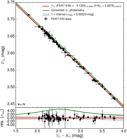
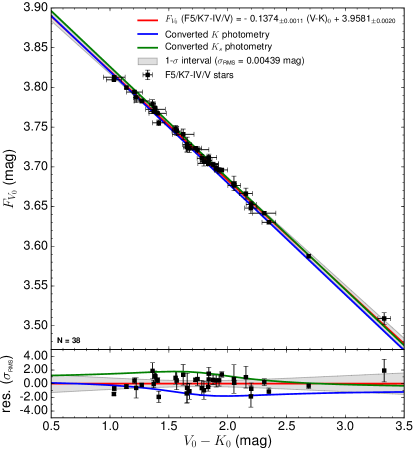
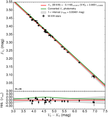
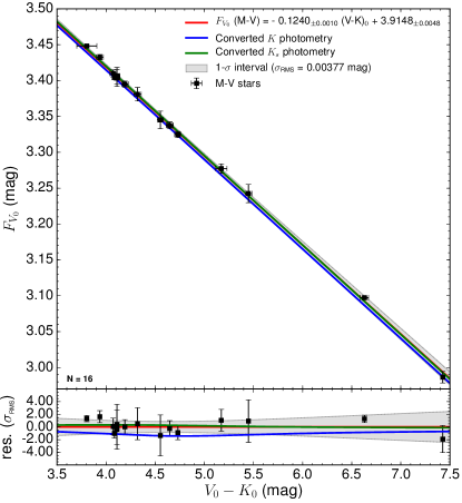
Figure 5: SBCRs for late-type stars using a converted photometric set for each sample, plotted above the data (black squares). Relations with converted Johnson $K$-photometries are shown as a blue solid line, while 2MASS $K_{s}$ ones are in a green solid line. See Sect. 6.1 for more information.

6.1 Update on late-type SBCRs

In Paper I, we implemented SBCRs using Gaia photometry. We noticed an error in the extinction calculation for the $G$-band. Indeed, Eq. 11 from Paper 1 should have been rewritten in the following way (Danielski et al., 2018):

$$A_{G}=A_{V}\times(a_{1}+a_{2}(G-K)_{0}+a_{3}(G-K)_{0}^{2}+a_{4}(G-K)_{0}^{3}\\ +a_{5}A_{V}+a_{6}A_{V}^{2}+a_{7}(G-K)_{0}A_{V}),$$ (7)

with $a_{1}=0.935556283,a_{2}=-0.090722012,a_{3}=0.014422056,a_{4}=-0.002659072,a_{5}=-0.030029634,a_{6}=0.000607315,$ and $a_{7}=0.002713748$. The converted SBCRs using the Gaia photometry are shown in Fig. 4, together with their parameters in Table 10. The expected precision on the angular diameter ranges from 1.1% to 2.5%.

We also propose to improve the calibration of our SBCRs for late-type stars obtained in papier I by using transformation equations to build a uniform infrared photometry set. We used Eq. A1 from Carpenter (2001), namely $K_{s}=K-0.044\,$mag, to transform our photometric sets. The resulting SBCRs are shown in Fig. 5 for each sample (i.e., F5/K7-II/III, F5/K7-IV/V, M-II/III, and M-V stars). Their parameters are included in Table 5. The angular diameter precision ranges from 1.0% to 2.7%.

Table 4: Parameters of the new converted SBCRs for late-type stars calibrated with Gaia photometry.

		$N_{c}$ /$N$	SBCR $F_{G_{0}}$ vs. $(G-K)_{0}$	$(G-K)$ range	$\sigma_{\mathrm{RMS}}$	Expected $\frac{\sigma{\theta_{\mathrm{LD}}}}{\theta_{\mathrm{LD}}}$
				[mag]	[mag]	[%]
F5/K7-II/III	Paper I		$F_{G_{0}}=-0.1289_{\pm 0.0010}(G-K)_{0}+3.9341_{\pm 0.0022}$	[1.6; 3.1]	0.00244	1.12
	$K$	0/69	$F_{G_{0}}=-0.1289_{\pm 0.0010}(G-K)_{0}+3.9341_{\pm 0.0022}$	[1.6; 3.1]	0.00244	1.12
	$K_{s}$	69/69	$F_{G_{0}}=-0.1289_{\pm 0.0010}(G-K_{s})_{0}+3.9398_{\pm 0.0022}$	[1.7; 3.2]	0.00244	1.12
F5/K7-IV/V	Paper I		$F_{G_{0}}=-0.1436_{\pm 0.0017}(G-K)_{0}+3.9587_{\pm 0.0027}$	[0.8; 2.7]	0.00494	2.27
	$K$	16/38	$F_{G_{0}}=-0.1472_{\pm 0.0015}(G-K)_{0}+3.9604_{\pm 0.0025}$	[0.8; 2.7]	0.00494	2.27
	$K_{s}$	22/38	$F_{G_{0}}=-0.1472_{\pm 0.0015}(G-K_{s})_{0}+3.9669_{\pm 0.0024}$	[0.8; 2.8]	0.00494	2.27
M-II/III	Paper I		$F_{G_{0}}=-0.1295_{\pm 0.0025}(G-K)_{0}+3.9324_{\pm 0.0088}$	[2.9; 4.9]	0.00543	2.50
	$K$	0/24	$F_{G_{0}}=-0.1295_{\pm 0.0025}(G-K)_{0}+3.9324_{\pm 0.0088}$	[2.9; 4.9]	0.00543	2.50
	$K_{s}$	24/24	$F_{G_{0}}=-0.1295_{\pm 0.0025}(G-K_{s})_{0}+3.9381_{\pm 0.0089}$	[3.0; 4.9]	0.00543	2.50
M-IV/V	Paper I		$F_{G_{0}}=-0.1388_{\pm 0.0028}(G-K)_{0}+3.9393_{\pm 0.0093}$	[3.0; 4.6]	0.00382	1.76
	$K$	13/15	$F_{G_{0}}=-0.1416_{\pm 0.0021}(G-K)_{0}+3.9444_{\pm 0.0069}$	[3.0; 4.6]	0.00407	1.87
	$K_{s}$	2/15	$F_{G_{0}}=-0.1416_{\pm 0.0021}(G-K_{s})_{0}+3.9506_{\pm 0.0069}$	[3.0; 4.6]	0.00407	1.87

Table 5: Parameters of the SBCRs for late-type stars described in Paper I, but converted into the same photometric system (see Sect. 6.1).

		$N_{c}$ /$N$	SBCR $F_{V_{0}}$ vs. $(V-K)_{0}$	$(V-K)$ range	$\sigma_{\mathrm{RMS}}$	Expected $\frac{\sigma{\theta_{\mathrm{LD}}}}{\theta_{\mathrm{LD}}}$
				[mag]	[mag]	[%]
F5/K7-II/III	$K$	0/70	$F_{V_{0}}=-0.1220_{\pm 0.0006}(V-K)_{0}+3.9278_{\pm 0.0016}$	[1.8; 3.8]	0.00223	1.03
	$K_{s}$	70/70	$F_{V_{0}}=-0.1220_{\pm 0.0006}(V-K_{s})_{0}+3.9332_{\pm 0.0016}$	[1.8; 3.9]	0.00223	1.03
F5/K7-IV/V	$K$	16/38	$F_{V_{0}}=-0.1404_{\pm 0.0014}(V-K)_{0}+3.9603_{\pm 0.0025}$	[1.0; 3.4]	0.00575	2.65
	$K_{s}$	22/38	$F_{V_{0}}=-0.1404_{\pm 0.0014}(V-K_{s})_{0}+3.9665_{\pm 0.0025}$	[1.0; 3.4]	0.00575	2.65
M-II/III	$K$	0/29	$F_{V_{0}}=-0.1165_{\pm 0.0012}(V-K)_{0}+3.9051_{\pm 0.0055}$	[3.7; 7.0]	0.00461	2.12
	$K_{s}$	29/29	$F_{V_{0}}=-0.1165_{\pm 0.0012}(V-K_{s})_{0}+3.9102_{\pm 0.0055}$	[3.7; 7.0]	0.00461	2.12
M-IV/V	$K$	14/16	$F_{V_{0}}=-0.1247_{\pm 0.0009}(V-K)_{0}+3.9133_{\pm 0.0044}$	[3.8; 7.4]	0.00404	1.86
	$K_{s}$	2/16	$F_{V_{0}}=-0.1247_{\pm 0.0009}(V-K_{s})_{0}+3.9188_{\pm 0.0044}$	[3.8; 7.4]	0.00404	1.86

6.2 Connecting late-type to early-type SBCRs

Our F5/K7-IV/V SBCR covers a color range from $V-K=1\,$mag to $V-K=2.7\,$mag, while our SBCR for early-type dwarf stars is valid up to $V-K=0.6\,$mag. There is therefore a gap in the validity domain of our relations between $V-K=0.6\,$mag and $V-K=1\,$mag. One way to solve this problem would be to merge both samples and deduce a unique SBCR. The methodology used to develop both SBCRs differs regarding the interferometric measurements we have selected to calibrate the relations. The SBCR for early-tpe stars is a homogeneous relation calibrated using measurements from a single instrument, namely VEGA. On the other hand, SBCRs for late-type stars were implemented with measurements taken from different instruments. Also, we have shown in Paper I that SBCRs depend on the spectral type of stars, where we raised strong discrepancies between M stars and F5/K7 stars. We thus made the choice not to calibrate a single SBCR for early- and late-type stars to avoid any systematics due to a mix of spectral types, and also due to a mix of uniform and inhomogeneous sets of interferometric measurements. By extending our F5/K7-IV/V SBCR as calibrated in Paper I (based on $K$ and $K_{s}$ photometry) until $V-K=0.6\,$mag, we find a difference of $2\sigma$ between both early-type (using $K$/$K_{s}$) and late-type relations. They are however consistent in the error bars at 1$\sigma$. The same result is found when comparing consistently uniform $K$ and $K_{s}$ SBCRs, respectively. We expect the CHARA/SPICA instrument to solve this gap by providing more F0 to F5 measurements.

7 Conclusions and perspectives

We carefully selected 18 early-type stars according to selection criteria in order to measure their angular diameter with the VEGA combiner at the CHARA Array interferometer. The mean precision we obtain on our angular diameter measurements is 2%. Using our SBCR leads to an expected statistical precision of 2.3% on the derived angular diameter, but the user should take care of photometric conversion issues discussed in Sect 5.2.

This work supports the results shown by Paper I. Indeed, to reach such statistical precision, we demonstrated the necessity of implementing selection criteria in order to calibrate the SBCRs. We also showed the need of including the $V-K$ uncertainties in the fitting process. In Paper I, we showed that SBCRs for late-type stars depend on the class of stars. In this work, and as a first step, we considered only dwarfs and subgiants stars. We also improved SBCRs for late-type stars presented in Paper I by converting the photometric data into the same system, and also by correcting the calculation of the extinction in the Gaia band.

The lack of a large set of homogeneous angular diameter interferometric measurements remains a major problem in the implementation of SBCRs. With the future SPICA instrument (Mourard et al., 2018) that will be installed at the CHARA array, we expect to derive the angular diameter of 800 stars all over the HR diagram, with a 1% precision level. CHARA/SPICA will also study rotation, multiplicity, wind, and environment by performing images in the visible domain. That should therefore reinforce our knowledge of SBCRs for early-type stars and in particular help to better understand the impact of stellar activity.

Appendix A VEGA visibility curves

Appendix B Observing log

Table 6: VEGA observing log of the 18 early-type stars. The columns list the date, the hour angle HA, the mean, the minimum, and the maximum wavelengths over which the squared visibility is calculated, the projected baseline length $B_{p}$, its orientation Arg, and the signal-to-noise ratio (S/N). The last column provides the calibrated squared visibility $V_{\mathrm{cal}}^{2}$ together with the statistic and the systematic errors. The data are available on the Jean-Marie Mariotti Center OiDB service (available at http://oidb.jmmc.fr). The interferometric observations are desribed in Sect. 3.

Star	Date	Peak	HA	$\lambda$	$\lambda_{\mathrm{min}}$	$\lambda_{\mathrm{max}}$	$B_{p}$	Arg	S/N	$V^{2}_{\mathrm{cal}_{\pm\mathrm{stat}\pm\mathrm{syst}}}$
	[yyyy.mm.dd]		[h]	[nm]	[nm]	[nm]	[m]	[deg]
HD11415	2019.10.07	1	3.39	710	700	720	65.87	-165.17	15.33	0.922 ±0.114±0.003
	2019.10.07	1	3.40	730	720	740	65.87	-165.27	20.17	0.898 ±0.045±0.004
	2019.10.07	1	3.79	730	720	740	65.87	-170.48	12.92	0.925 ±0.072±0.005
	2019.10.07	1	4.14	730	720	740	65.86	-175.28	18.26	0.932 ±0.051±0.004
	2019.10.07	1	4.53	730	720	740	65.86	179.49	11.13	0.939 ±0.084±0.004
	2020.07.18	1	-3.41	730	720	740	219.83	-51.60	5.60	0.353 ±0.063±0.007
	2020.07.18	1	-2.50	730	720	740	229.86	-65.39	5.26	0.286 ±0.054±0.005
	2020.07.19	1	-6.57	730	720	740	241.34	34.36	7.29	0.197 ±0.027±0.017
	2020.07.19	1	-5.50	730	720	740	244.59	21.34	5.29	0.180 ±0.034±0.015
	2020.07.19	1	-4.98	730	720	740	245.45	14.99	3.33	0.225 ±0.067±0.019
	2020.07.20	1	-1.90	730	720	740	142.75	-89.44	11.57	0.613 ±0.053±0.015
HD114330	2019.02.23	1	0.94	730	720	740	182.53	12.90	4.48	0.442 ±0.099±0.025
	2019.02.23	1	2.18	710	700	720	177.66	-2.94	6.54	0.535 ±0.082±0.032
	2019.02.23	1	2.21	730	720	740	177.73	-3.34	7.09	0.566 ±0.080±0.024
	2019.02.23	1	2.68	710	700	720	180.08	-9.39	7.49	0.545 ±0.073±0.033
	2019.02.23	1	2.70	730	720	740	180.21	-9.61	6.96	0.522 ±0.075±0.022
	2020.03.04	1	-0.41	705	695	715	62.90	-114.85	17.61	0.853 ±0.048±0.005
	2020.03.04	1	-0.41	725	715	735	62.90	-114.85	14.76	0.809 ±0.055±0.002
	2020.03.04	1	-0.08	705	695	715	61.16	-115.11	11.59	0.829 ±0.061±0.002
	2020.03.04	1	-0.08	725	715	735	61.16	-115.11	9.20	0.863 ±0.077±0.002
	2020.03.07	1	-1.26	725	715	735	65.54	-114.99	10.20	0.858 ±0.084±0.005
	2020.03.07	1	-0.42	705	695	715	62.96	-114.84	17.71	0.903 ±0.051±0.011
	2020.03.07	1	-0.42	725	715	735	62.96	-114.84	9.01	0.848 ±0.094±0.002
HD145389	2019.05.02	1	2.22	730	720	740	151.21	-141.88	6.65	0.586 ±0.088±0.008
	2019.05.02	1	2.69	710	700	720	149.07	-147.98	9.56	0.614 ±0.094±0.008
	2019.05.02	1	2.68	730	720	740	149.11	-147.84	11.63	0.642 ±0.055±0.010
	2019.05.02	1	2.98	710	700	720	147.74	-151.96	12.80	0.590 ±0.046±0.009
	2019.05.02	1	3.00	730	720	740	147.66	-152.22	7.14	0.605 ±0.085±0.009
	2020.03.04	1	-1.86	725	715	735	61.42	-105.17	11.66	0.914 ±0.078±0.002
HD145570	2019.06.14	1	-0.78	710	700	720	154.56	-110.12	9.34	0.631 ±0.069±0.013
	2019.06.17	1	-1.96	710	700	720	154.79	-113.22	11.50	0.619 ±0.054±0.010
	2019.06.17	2	-1.94	710	700	720	83.50	87.05	5.14	0.807 ±0.157±0.006
	2019.06.17	1	-1.62	710	700	720	156.03	-112.12	6.60	0.598 ±0.091±0.010
	2019.06.17	2	-1.53	710	700	720	90.32	88.32	13.09	0.871 ±0.067±0.004
	2019.06.17	1	-1.22	710	700	720	156.14	-111.08	9.13	0.592 ±0.065±0.009
	2019.06.17	2	-1.21	710	700	720	94.85	89.21	8.81	0.784 ±0.089±0.004
	2019.06.17	2	-0.86	710	700	720	99.11	90.15	5.86	0.858 ±0.147±0.006
HD148112	2019.06.15	1	-1.77	730	720	740	151.68	-108.73	8.61	0.662 ±0.105±0.033
	2019.06.15	1	-1.20	730	720	740	155.38	-110.31	9.89	0.612 ±0.062±0.026
	2019.06.15	1	-0.68	730	720	740	156.24	-112.09	9.80	0.647 ±0.066±0.032
	2019.08.16	1	4.37	710	700	720	33.77	145.58	12.78	1.002 ±0.078±0.002
	2019.08.16	1	4.39	730	720	740	33.76	145.54	14.82	0.995 ±0.067±0.002
HD149438	2019.06.17	1	-0.12	710	700	720	144.32	-102.73	13.50	0.758 ±0.047±0.010
	2019.06.17	1	0.27	710	700	720	138.51	-100.46	16.78	0.791 ±0.047±0.010
	2019.06.17	1	0.28	730	720	740	138.35	-100.40	10.72	0.799 ±0.075±0.013
	2019.06.17	1	1.52	710	700	720	112.40	-92.91	15.05	0.875 ±0.049±0.011
	2019.06.17	1	1.52	730	720	740	112.27	-92.88	8.79	0.816 ±0.093±0.014
	2020.03.05	1	-0.04	705	695	715	131.76	36.02	12.03	0.737 ±0.082±0.011
HD152107	2019.06.15	1	0.91	710	700	720	155.89	-126.31	8.65	0.627 ±0.073±0.013
	2019.06.15	1	0.89	730	720	740	155.91	-126.155	8.33	0.614 ±0.074±0.010
	2019.06.15	1	1.53	710	700	720	154.36	-133.49	8.40	0.633 ±0.075±0.010
	2019.06.15	1	1.52	730	720	740	154.39	-133.41	11.92	0.610 ±0.051±0.009
	2020.03.04	1	-1.09	705	695	715	63.97	-112.32	9.26	0.935 ±0.101±0.002
	2020.03.04	1	-1.09	725	715	735	63.96	-112.30	4.81	0.873 ±0.182±0.002
	2020.03.04	1	-0.56	705	695	715	65.10	-117.60	12.67	0.905 ±0.071±0.003
	2020.03.04	1	-0.56	725	715	735	65.09	-117.54	9.07	0.856 ±0.094±0.002
HD192640	2019.07.06	1	0.79	710	700	720	176.39	-27.36	5.96	0.413 ±0.094±0.005
	2019.07.06	1	0.79	730	720	740	176.39	-27.38	6.88	0.427 ±0.062±0.005
	2019.07.06	1	1.17	730	720	740	175.53	-30.27	8.47	0.438 ±0.052±0.005
	2019.08.15	1	2.47	730	720	740	33.15	151.85	13.76	0.933 ±0.052±0.001
	2019.08.15	2	2.47	730	720	740	201.98	-37.34	5.97	0.383 ±0.064±0.006
	2019.08.16	1	1.75	710	700	720	33.59	156.70	17.96	1.002 ±0.044±0.001
	2019.08.16	1	1.74	730	720	740	33.60	156.77	11.38	0.972 ±0.085±0.001
	2019.08.16	1	2.36	710	700	720	33.23	152.55	23.78	0.979 ±0.041±0.001
	2019.08.16	1	2.33	730	720	740	33.25	152.72	19.09	0.952 ±0.050±0.001
HD195810	2019.07.06	1	1.67	710	700	720	174.90	-33.63	12.65	0.571 ±0.073±0.010
	2019.07.06	1	1.66	730	720	740	174.86	-33.57	7.17	0.625 ±0.087±0.011
	2019.07.06	1	2.09	710	700	720	176.42	-35.59	11.32	0.566 ±0.050±0.011
	2019.07.06	1	2.08	730	720	740	176.40	-35.56	7.55	0.580 ±0.077±0.010
	2019.07.06	1	2.43	710	700	720	177.17	-36.93	9.82	0.585 ±0.060±0.013
	2019.07.06	1	2.43	730	720	740	177.17	-36.93	8.89	0.589 ±0.066±0.011
	2019.08.17	1	2.99	710	700	720	33.92	149.87	23.50	0.986 ±0.042±0.001
	2019.08.17	1	3.00	730	720	740	33.92	149.82	19.92	0.990 ±0.050±0.001
HD27819	2019.10.07	1	-2.12	730	720	740	63.50	-112.26	17.10	0.851 ±0.050±0.008
	2019.10.07	1	-1.70	730	720	740	64.91	-113.64	10.64	0.871 ±0.082±0.007
	2019.10.07	1	-1.29	730	720	740	65.67	-115.17	11.30	0.915 ±0.081±0.008
	2019.10.09	1	-0.89	710	700	720	242.78	25.72	8.39	0.212 ±0.025±0.031
	2019.10.09	1	-0.88	730	720	740	242.71	25.63	6.94	0.196 ±0.028±0.028
	2019.10.09	1	-0.50	710	700	720	240.55	22.80	6.89	0.238 ±0.035±0.033
	2019.10.09	1	-0.51	730	720	740	240.58	22.84	12.26	0.206 ±0.017±0.028
	2019.10.09	1	-0.08	710	700	720	238.10	19.40	8.07	0.226 ±0.026±0.028
	2019.10.09	1	0.39	710	700	720	235.49	15.25	8.39	0.176 ±0.020±0.022
	2019.10.09	1	0.38	730	720	740	235.52	15.31	11.87	0.184 ±0.015±0.024
HD27962	2019.10.07	1	-0.90	710	700	720	65.87	-116.84	8.26	0.817 ±0.099±0.010
	2019.10.07	1	-0.92	730	720	740	65.87	-116.77	12.64	0.885 ±0.070±0.009
	2019.10.07	1	-0.45	710	700	720	65.52	-119.09	14.64	0.864 ±0.059±0.009
	2019.10.07	1	-0.45	730	720	740	65.51	-119.11	9.38	0.866 ±0.092±0.007
	2019.10.07	1	0.10	710	700	720	64.24	-122.33	16.21	0.962 ±0.059±0.010
	2019.10.10	1	-1.67	710	700	720	165.56	-6.20	1.81	0.432 ±0.040±0.019
	2019.10.10	1	-1.67	720	700	740	165.56	-6.17	5.53	0.314 ±0.057±0.019
	2020.12.16	1	-1.51	710	700	720	93.93	105.62	8.24	0.700 ±0.085±0.023
	2020.12.16	1	-0.88	710	700	720	100.92	101.70	9.30	0.747 ±0.080±0.017
	2020.12.16	1	-0.89	730	720	740	100.89	101.72	14.54	0.739 ±0.051±0.021
	2020.12.16	1	-0.22	710	700	720	105.76	98.17	9.23	0.686 ±0.074±0.016
	2020.12.16	1	-0.23	730	720	740	105.74	98.19	18.87	0.690 ±0.037±0.020
	2020.12.16	1	0.50	710	700	720	107.88	94.72	14.49	0.716 ±0.049±0.020
HD3360	2019.08.15	1	-0.68	710	700	720	32.08	175.73	11.37	0.939 ±0.083±0.001
	2019.08.15	2	-0.71	710	700	720	201.90	-13.57	6.21	0.591 ±0.091±0.007
	2019.08.15	1	-0.70	730	720	740	32.09	175.85	19.57	0.952 ±0.049±0.001
	2019.08.16	1	-1.26	730	720	740	32.11	-179.09	13.46	1.018 ±0.076±0.001
	2019.08.16	2	-1.26	730	720	740	202.87	-8.25	9.36	0.624 ±0.067±0.011
	2020.08.26	1	-2.75	705	695	715	133.59	-83.32	15.32	0.806 ±0.053±0.005
	2020.08.26	1	-1.96	705	695	715	142.47	-93.06	18.79	0.742 ±0.039±0.010
	2020.08.26	1	-1.96	725	715	735	142.47	-93.06	24.95	0.771 ±0.031±0.010
	2020.08.26	1	-1.40	705	695	715	147.43	-99.61	25.44	0.765 ±0.030±0.015
	2020.08.26	1	-1.40	725	715	735	147.43	-99.61	24.16	0.741 ±0.031±0.013
	2020.08.26	1	-1.00	725	715	735	150.34	-104.32	22.90	0.760 ±0.033±0.014
	2020.08.26	1	0.13	705	695	715	155.25	-117.31	12.55	0.687 ±0.055±0.012
	2020.08.36	1	0.13	725	715	735	155.25	-117.31	22.27	0.695 ±0.031±0.009
	2020.08.29	1	-1.94	710	700	720	171.79	-3.35	7.91	0.629 ±0.080±0.015
	2020.08.30	1	-0.87	710	700	720	151.08	-105.72	7.99	0.697 ±0.087±0.011
	2020.08.30	1	-0.26	710	700	720	154.04	-112.78	23.36	0.709 ±0.030±0.015
	2020.08.30	1	-0.26	730	720	740	154.04	-112.78	20.52	0.718 ±0.035±0.012
	2020.08.30	1	0.18	730	720	740	155.36	-117.88	20.73	0.732 ±0.035±0.010
HD33959	2019.08.17	1	-3.64	710	700	720	34.00	-159.96	11.11	0.980 ±0.088±0.001
	2019.08.17	1	-3.65	730	720	740	34.00	-159.95	13.75	0.996 ±0.072±0.001
	2019.08.17	1	-3.26	710	700	720	34.05	-162.80	14.53	0.989 ±0.068±0.001
	2019.08.17	2	-3.24	710	700	720	210.32	10.48	8.18	0.255 ±0.031±0.004
	2019.08.17	1	-3.27	730	720	740	34.05	-162.76	14.37	1.007 ±0.070±0.001
	2019.08.17	2	-3.24	730	720	740	210.31	10.42	16.78	0.256 ±0.015±0.004
	2019.08.17	1	-2.81	710	700	720	34.07	-166.35	10.39	0.963 ±0.093±0.001
	2019.08.17	1	-2.83	730	720	740	34.07	-166.15	11.85	0.925 ±0.078±0.001
	2019.08.17	2	-2.82	730	720	740	210.06	6.55	3.78	0.297 ±0.079±0.005
	2020.08.26	1	-3.41	705	695	715	120.39	-91.44	22.24	0.629 ±0.028±0.056
	2020.08.26	1	-2.97	705	695	715	129.56	-94.82	21.21	0.575 ±0.027±0.084
	2020.08.26	1	-2.97	725	715	735	129.56	-94.82	18.09	0.630 ±0.035±0.072
	2020.08.26	1	-2.61	705	695	715	135.92	-97.39	25.38	0.613 ±0.024±0.071
	2020.08.26	1	-2.61	725	715	735	135.92	-97.39	16.74	0.591 ±0.035±0.005
	2020.08.26	1	-2.18	705	695	715	142.58	-100.48	21.21	0.568 ±0.027±0.083
	2020.08.26	1	-2.18	725	715	735	142.58	-100.48	19.17	0.554 ±0.029±0.068
HD35468	2019.10.05	1	-1.20	710	700	720	65.85	-115.71	18.80	0.786 ±0.042±0.004
	2019.10.05	1	-1.19	730	720	740	65.85	-115.72	21.47	0.712 ±0.033±0.003
	2019.10.05	1	-0.73	730	720	740	65.27	-116.74	18.46	0.768 ±0.042±0.003
	2019.10.05	1	0.08	730	720	740	62.49	-119.41	25.37	0.801 ±0.032±0.003
	2020.08.30	1	-3.28	710	700	720	131.90	-111.05	13.14	0.278 ±0.021±0.017
	2020.08.30	1	-3.29	730	720	740	131.81	-111.06	13.84	0.272 ±0.020±0.017
	2020.08.30	1	-2.77	710	700	720	141.22	-110.42	10.25	0.209 ±0.020±0.020
	2020.08.30	1	-2.77	730	720	740	141.28	-110.41	8.12	0.243 ±0.030±0.004
	2020.08.30	1	-2.33	710	700	720	147.69	-110.21	10.09	0.189 ±0.019±0.018
	2020.08.30	1	-2.32	730	720	740	147.80	-110.21	8.17	0.220 ±0.027±0.004
	2020.08.30	1	-1.88	710	700	720	152.37	-110.29	11.20	0.182 ±0.016±0.017
	2020.08.30	1	-1.88	730	720	740	152.37	-110.29	15.35	0.154 ±0.010±0.003
HD58142	2019.02.23	1	1.07	710	700	720	243.55	8.38	2.58	0.265 ±0.103±0.006
	2019.02.23	1	1.66	710	700	720	244.00	2.83	3.37	0.259 ±0.077±0.008
	2019.02.23	1	1.66	730	720	740	244.00	2.77	4.75	0.296 ±0.062±0.011
	2019.02.23	1	2.14	710	700	720	244.03	-1.76	3.56	0.266 ±0.075±0.009
	2019.02.23	1	2.63	710	700	720	243.76	-6.49	2.12	0.199 ±0.094±0.007
	2019.02.23	1	2.62	730	720	740	243.77	-6.34	3.50	0.248 ±0.111±0.012
	2020.03.07	1	1.83	705	695	715	65.319	-144.30	12.88	0.961 ±0.075±0.008
	2020.03.07	2	1.83	705	695	715	154.43	-137.53	5.42	0.670 ±0.124±0.037
	2020.03.07	1	1.83	725	715	735	65.322	-144.25	10.16	0.923 ±0.091±0.004
	2020.03.07	2	1.83	725	715	735	154.43	-137.53	11.41	0.650 ±0.057±0.037
	2020.03.07	1	2.43	705	695	715	64.76	-151.88	13.43	0.953 ±0.071±0.008
	2020.03.07	2	2.43	705	695	715	152.58	-145.25	13.37	0.691 ±0.052±0.037
	2020.03.07	2	2.43	725	715	735	152.58	-145.25	10.00	0.654 ±0.065±0.044
HD886	2019.08.20	1	1.42	730	720	740	175.54	-31.95	17.64	0.531 ±0.030±0.005
	2019.08.20	1	1.95	710	700	720	176.97	-34.74	8.98	0.518 ±0.058±0.005
	2019.08.20	1	1.95	730	720	740	176.97	-34.74	18.83	0.480 ±0.025±0.004
	2019.08.20	1	2.49	710	700	720	177.44	-37.09	9.13	0.504 ±0.055±0.005
	2019.08.20	1	2.49	730	720	740	177.44	-37.09	16.47	0.518 ±0.031±0.005
	2019.08.21	1	2.48	710	700	720	177.44	-37.05	11.85	0.521 ±0.044±0.005
	2019.08.21	1	2.48	730	720	740	177.44	-37.05	8.78	0.535 ±0.061±0.005
	2019.08.22	1	1.97	710	700	720	177.02	-34.86	23.36	0.519 ±0.022±0.005
	2019.08.22	1	1.97	730	720	740	177.02	-34.86	17.84	0.508 ±0.028±0.005
	2019.08.22	1	2.28	710	700	720	177.39	-36.26	20.02	0.506 ±0.025±0.005
	2019.08.22	1	2.28	730	720	740	177.39	-36.24	17.81	0.492 ±0.028±0.004
	2019.08.22	1	2.63	710	700	720	177.37	-37.62	16.20	0.528 ±0.033±0.005
	2019.08.22	1	2.63	730	720	740	177.37	-37.62	16.68	0.520 ±0.031±0.005
HD89021	2019.02.26	1	1.99	710	700	720	64.05	-145.57	8.43	0.760 ±0.069±0.007
	2019.02.26	2	2.00	710	700	720	151.20	-138.74	7.89	0.182 ±0.060±0.007
	2019.02.26	1	2.00	730	720	740	64.04	-145.63	5.66	0.763 ±0.135±0.006
	2019.02.26	2	2.00	730	720	740	151.20	-138.74	3.17	0.249 ±0.079±0.010
	2019.02.26	2	2.50	710	700	720	148.56	-145.21	7.36	0.262 ±0.050±0.007
	2020.06.15	1	4.88	710	700	720	140.52	179.97	8.83	0.240 ±0.027±0.002
	2020.06.15	1	4.89	730	720	740	140.52	179.75	7.65	0.280 ±0.037±0.003
	2020.06.15	1	5.35	710	700	720	140.91	172.67	8.54	0.250 ±0.017±0.002
	2020.06.15	1	5.34	730	720	740	140.90	172.78	7.76	0.269 ±0.035±0.002
	2020.12.19	1	-0.15	710	700	720	107.28	101.47	7.04	0.588 ±0.083±0.045
	2020.12.20	1	-0.14	730	720	740	107.31	101.33	5.28	0.546 ±0.104±0.020
	2020.12.21	1	0.80	730	720	740	107.62	91.73	7.59	0.530 ±0.070±0.021
HD97633	2019.05.03	1	1.13	710	700	720	142.96	-122.06	8.38	0.252 ±0.030±0.007
	2019.05.03	1	1.59	710	700	720	136.12	-125.81	8.83	0.304 ±0.041±0.009
	2019.05.03	1	1.60	730	720	740	136.02	-125.87	14.95	0.257 ±0.017±0.006
	2019.05.03	1	2.01	710	700	720	129.31	-129.75	8.94	0.309 ±0.052±0.013
	2019.05.03	1	2.01	730	720	740	129.25	-129.78	9.18	0.372 ±0.040±0.013
	2020.12.16	1	-2.35	710	700	720	80.64	110.16	14.83	0.688 ±0.046±0.031
	2020.12.16	1	-2.35	730	720	740	80.59	110.18	17.82	0.673 ±0.038±0.029
	2020.12.16	1	-1.74	710	700	720	90.23	105.65	24.23	0.636 ±0.026±0.029
	2020.12.16	1	-1.74	730	720	740	90.23	105.65	26.70	0.646 ±0.024±0.028
	2020.12.16	1	0.14	710	700	720	107.21	96.11	12.62	0.477 ±0.038±0.022
	2020.12.16	1	0.14	730	720	740	107.21	96.11	23.73	0.463 ±0.020±0.020
	2020.12.16	1	0.61	710	700	720	107.92	94.19	13.77	0.432 ±0.031±0.019
	2020.12.16	1	0.62	730	720	740	107.91	94.18	21.60	0.454 ±0.021±0.019

Table 6: Continued.