Testing Group Fairness via Optimal Transport Projections

Abstract

We present a statistical testing framework to detect if a given machine learning classifier fails to satisfy a wide range of group fairness notions. The proposed test is a flexible, interpretable, and statistically rigorous tool for auditing whether exhibited biases are intrinsic to the algorithm or due to the randomness in the data. The statistical challenges, which may arise from multiple impact criteria that define group fairness and which are discontinuous on model parameters, are conveniently tackled by projecting the empirical measure onto the set of group-fair probability models using optimal transport. This statistic is efficiently computed using linear programming and its asymptotic distribution is explicitly obtained. The proposed framework can also be used to test for testing composite fairness hypotheses and fairness with multiple sensitive attributes. The optimal transport testing formulation improves interpretability by characterizing the minimal covariate perturbations that eliminate the bias observed in the audit.

1 Introduction

Algorithmic decisions are commonly conceived to have the potential of being more objective than a human’s decisions, since they are generated by logical instructions and the rules of algebra. However, recent studies indicate that this may not be the case. For example, an algorithm which helps the US criminal justice system to predict recidivism rates has been shown to falsely give a higher risk for African-Americans than white Americans (Chouldechova, 2017; MultiMedia LLC, 2016). Similar biases are exhibited against female candidates in a hiring-help system developed by Amazon AI (Dastin, 2018) and an ad-targeting algorithm used by Google (Datta et al., 2015).

A natural first explanation for the reported algorithmic biases is that the data used to train the algorithms may already be corrupted by human biases (Buolamwini & Gebru, 2018; Manrai et al., 2016). Deeper inquests have revealed insights on how common learning procedures intrinsically perpetuate the biases and potentially introduce fresh ones. The usual practice of training by minimizing empirical risk, while geared towards yielding predictions that are best when averaged over the entire population, often under-represents minority subgroups in the datasets. Moreover, even though certain sensitive attributes are forbidden by law to be used in the algorithm, the strong correlations between the sensitive attributes and other features potentially lead to biases in predictions. As reported in the studies in (Grgic-Hlaca et al., 2016; Garg et al., 2019; Barocas & Selbst, 2016; Black et al., 2020; Kleinberg et al., 2018; Lipton et al., 2018), merely masking the sensitive attributes does not address the problem.

The aforementioned biases and their impacts have sparked substantial interests in the pursuit of algorithmic fairness (Berk et al., 2018; Chouldechova & Roth, 2020; Corbett-Davies et al., 2017; Mehrabi et al., 2019). Testing whether a given machine learning algorithm is fair emerges as a question of first-order importance. In turn, designing this test for a wide range of group fairness notions (discussed in the sequel) is the main task of this paper.

Our proposed statistical hypothesis testing framework (testing framework for short) allows the auditors to systematically determine whether the biases exhibited in the audit procedure, if any, are intrinsic to the algorithm or due to the randomness in data. Moreover, our framework can be implemented as a black-box, without knowing the exact structure of the classification algorithm used.

For settings where sensitive attributes are not explicitly used as input to classification, fairness is measured on impact either at a group level or at an individual level (Barocas & Selbst, 2016). Group fairness notions seek to measure the differences in impacts across different groups and constitute the prominent means of assessing discrimination associated with group memberships. Individual fairness, on the other hand, seeks to assess if similar users are treated similarly (Dwork et al., 2012; John et al., 2020; Xue et al., 2020). Common examples of group fairness notions include disparate impact (Zafar et al., 2017), demographic parity (statistical parity) (Calders & Verwer, 2010), equality of opportunity (Hardt et al., 2016), equalized odds (Hardt et al., 2016), etc. The specific choice is usually driven by the philosophical, sociological or legal constraints binding the application considered.

Our testing framework applies to a generic notion of group fairness which encompasses all of the above specific group fairness notions as examples. This unifying approach can also be used in contexts requiring the use of different fairness notions simultaneously and settings with multiple groups.

Since a single fairness criterion among two groups can be reduced to testing the equality in two sample conditional means, one may consider employing a Welch’s $t$-test or a permutation test. Further, a suitable adjustment of the randomness in sample sizes, as in  DiCiccio et al. (2020); Tramer et al. (2017) can be applied. Some other existing methods such as Besse et al. (2018) also only apply to one-dimensional criterion. Extensions to multiple impact criteria are not immediate, as is the equalized odds case criterion (Hardt et al., 2016), or in the presence of multiple groups. Algorithmic approaches, such as in (Saleiro et al., 2018), lack the control of the type-I (false positive error). In contrast, the framework proposed here is applicable under general multiple impact criteria and controls the type-I error exactly.

The statistical challenges, which may arise from the presence of multiple impact criteria, are conveniently handled in our framework by utilizing the machinery of optimal transport projections. This involves computing the test statistic by projecting, or in other words, optimally transporting the empirical measure to the set of probability models which satisfy the group fairness notion (or notions) considered. This gives a measure of plausibility of the classifier in satisfying the fairness criterion under the data-generating distribution and the fairness hypothesis is duly rejected if the test statistic exceeds a suitable threshold determined by the significance level. This threshold is determined from the limiting distribution of the test statistic obtained as one of the main results of this paper.

Performing statistical inference with a projection criterion is prevalent in statistics: Owen (2001) serves as a comprehensive reference for projections, or profile functions, that are computed based on likelihood ratio metrics or the Kullback-Liebler divergence. Blanchet et al. (2019) and Cisneros-Velarde et al. (2020) study statistical inference with optimal transport projections. Recently, optimal transport divergences (Villani, 2008) become an attractive tool in many recent machine learning studies, including missing data imputation, geodesic PCA, point embeddings, and repairing data with Wasserstein barycenters for training fair classifiers  (Silvia et al., 2020; Gordaliza et al., 2019; Zehlike et al., 2020).

Taskesen et al. (2021) uses optimal transport projections to test a smooth relaxation of the equal opportunity criterion called probabilistic fairness; see Pleiss et al. (2017). This relaxation is required in Taskesen et al. (2021) to overcome the discontinuities in the classification boundaries which create technical complications when computing the optimal transport projections. Further, the resulting test statistic involves a non-convex optimization problem which is difficult to compute. In contrast, our work resolves the technical challenges arising from the discontinuities in classification boundaries. Moreover, our test statistic is the optimal value of a linear program, whose optimal solution offers interpretability by characterizing the minimal covariate perturbations that eliminate the bias observed in the audit. We emphasize that addressing boundary discontinuities is not simply a technical improvement. As we discuss in Section 3.3, our results show different qualitative behaviors both in the scaling and the interpretation of the optimal transport projection in terms of group fairness using optimal transport projections. In addition to enabling exact, computationally tractable, and interpretable fairness assessment for general deterministic classifiers, the technical analysis serves as a stepping stone for statistical inference in estimation tasks such as quantile regression which involve discontinuous estimating equations.

The main contributions are summarized as follows:

(1) We develop a statistical hypothesis test for assessing group fairness as per a generic notion that includes commonly used fairness criteria as special cases. The test is computationally tractable and interpretable. Besides being applicable to settings involving multiple groups, our framework is also applicable to any classifier algorithms, including but not limited to the logistic regression, SVMs, kernel methods, and nearest neighbors.

(2) We develop an extension of the statistical test for the testing problem with composite null hypothesis, addressed here as $\epsilon$-fairness.

(3) The framework facilitates the exact use of fairness criterion, thus obviating the need to invoke relaxations in the absence of smoothness in the impact criteria defining group fairness. The resulting qualitative difference, in terms of the rate of convergence for resulting optimal transport projections, is previously unreported and could be of interest from the technical standpoint of analysing profile functions with discontinuous score functions.

The remainder of the paper is structured as follows. In Section 2, we introduce a generic notion of group fairness and discuss the theory of optimal transport. Section 3 details the proposed statistical test for the simple fairness null hypothesis. Section 4 extends our approach to composite hypotheses. Section 5 discusses computational methods associated with the test. Numerical experiments presented in Section 6 serve to demonstrate the efficacy of the test. All technical proofs are relegated to Appendix A.

Notations. We use $\|\cdot\|_{*}$ to denote the dual norm of $\|\cdot\|$. We denote $(x)^{-}=\min\left\{x,0\right\}$ and $(x)^{+}=\max\{x,0\}$. We use $\Rightarrow$, $\overset{p}{\longrightarrow}$ and $\overset{a.s.}{\longrightarrow}$ to denote convergence in distribution, in probability and convergence almost surely, respectively. The support of the distribution of $X$ is represented by $\text{supp}(X)$. We use $[n]$ to denote the set $\{1,2,\ldots,n\}$ and $\mathbb{R}_{+}^{m}$ to denote the positive orthant $\{x\in\mathbb{R}_{+}^{m}:x\geq 0\}$. $\delta_{(x,a,y)}$ denotes a Dirac measure on a fixed point $(x,a,y)$.

2 Problem Setup and Preliminaries

Throughout this paper we consider the classification settings in which the deterministic classifier $\mathcal{C}:\mathcal{X}\rightarrow\mathcal{Y}$ maps the input features from $\mathcal{X}\subset\mathbb{R}^{d}$ to output labels in the set $\mathcal{Y}=\{0,1\}$. Evaluation of fairness is considered with respect to a sensitive attribute $A$ taking values in a finite set $\mathcal{A}.$ For simplicity, we consider $\mathcal{A}=\{0,1\}$ where $A=1$ can be taken to identify the reference group. The statistical test developed in this paper and the main results are applicable more generally to settings involving a non-binary sensitive attribute (or) multiple sensitive attributes. Most notions of group fairness are stated in terms of the joint distribution $\mathbb{Q}$ of $(X,A,Y),$ where $X$ is the vector of input features, $A$ is the sensitive attribute, and $Y$ is the class label of a random sample from the population.

2.1 Notions of Group Fairness

A general reference to fairness notions can be found in Makhlouf et al. (2020, Table 14). The statistical notion of group fairness that we consider, encapsulated in Definition 1 below, is stated flexibly to include commonly used notions such as equal opportunity (Hardt et al., 2016), predictive equality (Corbett-Davies et al., 2017), equalized odds (Hardt et al., 2016), and statistical parity (Dwork et al., 2012), etc., as special cases. This flexibility is achieved by stating the definition in terms of a tuple $(U,\phi),$ where $U$ is an $\mathbb{R}^{s}$-valued random vector completely dependent on $(A,Y)$ and $\phi:\mathbb{R}^{s}\times\mathbb{R}^{s}\to\mathbb{R}^{m}$ is a function chosen to discern the differences in performance of the classifier across groups. We address $(U,\phi)$ as the discerning tuple.

Definition 1 (Generic notion of group fairness).

A classifier $\mathcal{C}:\mathcal{X}\to\{0,1\}$ is fair with respect to the discerning tuple $(U,\phi)$ under a probability distribution $\mathbb{Q}$ if

$$\mathbb{E}_{\mathbb{Q}}[\mathcal{C}(X)\phi(U,\mathbb{E}_{\mathbb{Q}}[U])]=0.$$ (1)

Note that $\mathcal{C}(X)=\mathbb{I}\{\mathcal{C}(X)=1\}$, and thus equation (1) can be seen as $\mathbb{E}_{\mathbb{Q}}[\mathbb{I}\{\mathcal{C}(X)=1\}\phi(U,\mathbb{E}_{\mathbb{Q}}[U])]=0.$ At the first glance, equation (1) seems asymmetric as it only considers the positive prediction label $\mathcal{C}(X)=1$. However, it is easy to check that $\mathbb{E}_{\mathbb{Q}}[\phi(U,\mathbb{E}_{\mathbb{Q}}[U])]=0$ in all the group fairness notions in Examples 1 - 6. By taking the difference, we get the symmetric guarantee that $\mathbb{E}_{\mathbb{Q}}[\mathbb{I}\{\mathcal{C}(X)=0\}\phi(U,\mathbb{E}_{\mathbb{Q}}[U])]=0$.

Various useful notions of fairness can be obtained by varying the choice of $(U,\phi)$ as illustrated in Examples 1 - 6 below. We take $\mathcal{A}=\{0,1\}$ in Examples 1 - 4.

Example 1 (Equal opportunity (Hardt et al., 2016)).

A classifier $\mathcal{C}:\mathcal{X}\to\{0,1\}$ satisfies the equal opportunity criterion relative to a distribution $\mathbb{Q}$ if

$$\mathbb{Q}\left(\mathcal{C}(X)=1|A=1,Y=1\right)$$

$$\quad-\mathbb{Q}\left(\mathcal{C}(X)=1|A=0,Y=1\right)=0.$$

This criterion coincides with condition (1) with the choice $U=(\mathbb{I}_{(1,1)}(A,Y);\mathbb{I}_{(0,1)}(A,Y))$, where $\mathbb{I}_{(a,y)}(A,Y)$ denotes the indicator $\mathbb{I}(A=a,Y=y)$, and

$$\phi:(U,\mathbb{E}_{\mathbb{Q}}[U])\mapsto\frac{U_{1}}{\mathbb{E}_{\mathbb{Q}}[U_{1}]}-\frac{U_{2}}{\mathbb{E}_{\mathbb{Q}}[U_{2}]}.$$ (2)

Example 2 (Predictive equality (Corbett-Davies et al., 2017)).

A classifier $\mathcal{C}:\mathcal{X}\to\{0,1\}$ satisfies the predictive equality criterion relative to a distribution $\mathbb{Q}$ if

$$\mathbb{Q}\left(\mathcal{C}(X)=1|A=0,Y=0\right)$$

$$\quad-\mathbb{Q}\left(\mathcal{C}(X)=1|A=1,Y=0\right)=0.$$

This criterion coincides with condition (1) with the choice $U=[\mathbb{I}_{(1,0)}(A,Y);\mathbb{I}_{(0,0)}(A,Y)]$ and $\phi$ takes the same form as the function (2).

Example 3 (Equalized odds (Hardt et al., 2016)).

A classifier $\mathcal{C}:\mathcal{X}\to\{0,1\}$ satisfies the equalized odds criterion relative to a distribution $\mathbb{Q}$ if it satisfies both equal opportunity and predictive equality criteria. This criterion coincides with condition (1) with $U=[\mathbb{I}_{(1,1)}(A,Y);\mathbb{I}_{(0,1)}(A,Y);\mathbb{I}_{(1,0)}(A,Y);\mathbb{I}_{(0,0)}(A,Y)]$ and

$$\phi:(U,\mathbb{E}_{\mathbb{Q}}[U])\mapsto\Big{[}\frac{U_{1}}{\mathbb{E}_{\mathbb{Q}}[U_{1}]}-\frac{U_{2}}{\mathbb{E}_{\mathbb{Q}}[U_{2}]};\frac{U_{3}}{\mathbb{E}_{\mathbb{Q}}[U_{3}]}-\frac{U_{4}}{\mathbb{E}_{\mathbb{Q}}[U_{4}]}\Big{]}.$$

Example 4 (Statistical parity (Dwork et al., 2012)).

A classifier $\mathcal{C}:\mathcal{X}\to\{0,1\}$ satisfies the statistical parity criterion relative to a distribution $\mathbb{Q}$ if

$$\mathbb{Q}\left(\mathcal{C}(X)=1|A=1\right)-\mathbb{Q}\left(\mathcal{C}(X)=1|A=0\right)=0.$$

This criterion coincides with condition (1) with the choice $U=[\mathbb{I}_{1}(A);\mathbb{I}_{0}(A)]$ and $\phi$ takes the same form as the function (2).

If the sensitive attribute takes multiple values or there are multiple sensitive attributes, we can still define the associated fairness notions, which correspond to different choices of $(U,\phi)$.

Example 5 (Equal opportunity with a non-binary sensitive attribute).

Let $\mathcal{A}=\{0,1,2,\ldots,k\}$. A classifier $\mathcal{C}:\mathcal{X}\to\{0,1\}$ satisfies the equal opportunity criterion relative to a probability measure $\mathbb{Q}$ if

$$\mathbb{Q}\left(\mathcal{C}(X)=1|A=t,Y=1\right)$$

$$\quad-\mathbb{Q}\left(\mathcal{C}(X)=1|A=0,Y=1\right)=0\quad\forall t\in\mathcal{A}\backslash\{0\}.$$

This criterion coincides with condition (1) with the choice $U=(\mathbb{I}_{(0,1)}(A,Y);\mathbb{I}_{(1,1)}(A,Y);\ldots\mathbb{I}_{(k,1)}(A,Y))$ and $\phi=(\phi_{1},\phi_{2},\ldots,\phi_{t})$ with

$$\phi_{t}:(U,\mathbb{E}_{\mathbb{Q}}[U])\mapsto\frac{U_{t}}{\mathbb{E}_{\mathbb{Q}}[U_{t}]}-\frac{U_{1}}{\mathbb{E}_{\mathbb{Q}}[U_{1}]}\quad\forall t\in\mathcal{A}\backslash\{0\}.$$

Example 6 (Equal opportunity with multiple sensitive attributes).

Suppose we have $K$ sensitive attributes, $A_{1},A_{2},\ldots,A_{K}$, all taking values in a superset $\mathcal{A}$. A classifier $\mathcal{C}:\mathcal{X}\to\{0,1\}$ satisfies the equal opportunity criterion relative to a probability measure $\mathbb{Q}$ if

$$\mathbb{Q}\left(\mathcal{C}(X)=1|A_{t}=1,Y=1\right)$$

$$\quad-\mathbb{Q}\left(\mathcal{C}(X)=1|A_{t}=0,Y=1\right)=0\quad\forall t\in[K].$$

This criterion coincides with condition (1) with the choice

$$U_{t}=\mathbb{I}_{(1,1)}(A_{t},Y)\text{ and }U_{t+K}=\mathbb{I}_{(0,1)}(A_{t},Y)\quad\forall t\in[K]$$

and $\phi=(\phi_{1},\phi_{2},\ldots,\phi_{t})$ with

$$\phi_{t}:(U,\mathbb{E}_{\mathbb{Q}}[U])\mapsto\frac{U_{t}}{\mathbb{E}_{\mathbb{Q}}[U_{t}]}-\frac{U_{t+K}}{\mathbb{E}_{\mathbb{Q}}[U_{t+K}]}\quad\forall t\in[K].$$

2.2 Optimal Transport and the Wasserstein Distance

We next introduce the notion of optimal transport costs, of which Wasserstein distances is a special case. Let $P(\mathcal{Z})$ denote the set of all probability distributions on $\mathcal{Z}\triangleq\mathcal{X}\times\mathcal{A}\times\mathcal{Y}.$

Definition 2 (Optimal transport costs, Wasserstein distances).

Given a lower semicontinuous function $c:\mathcal{Z}\times\mathcal{Z}\rightarrow[0,\infty],$ the optimal transportation cost $W_{c}(\mathbb{Q}_{1},\mathbb{Q}_{2})$ between any two distributions $\mathbb{Q}_{1},\mathbb{Q}_{2}\in P(\mathcal{Z})$ is given by,

$$W_{c}(\mathbb{Q}_{1},\mathbb{Q}_{2})=\min_{\pi\in\Pi(\mathbb{Q}_{1},\mathbb{Q}_{2})}\mathbb{E}_{\pi}\left[{c}\left(Z,Z^{\prime}\right)\right],$$

where $\Pi(\mathbb{Q}_{1},\mathbb{Q}_{2})$ is the set of all joint distributions of $(Z,Z^{\prime})$ such that the law of $Z=(X,A,Y)$ is $\mathbb{Q}_{1}$ and that of $Z^{\prime}=(X^{\prime},A^{\prime},Y^{\prime})$ is $\mathbb{Q}_{2}.$

If $c(\cdot,\cdot)$ is a metric on $\mathcal{Z}$, then $W_{c}(\cdot)$ is the type-1 Wasserstein distance; see Villani (2008, Chapter 6). The quantity $W_{c}(\mathbb{Q}_{1},\mathbb{Q}_{2})$ can be interpreted as the least transportation cost incurred in transporting mass from $\mathbb{Q}_{1}$ to $\mathbb{Q}_{2},$ when the cost of transporting unit mass from location $z\in\mathcal{Z}$ to location $z^{\prime}\in\mathcal{Z}$ is given by $c(z,z^{\prime})$.

Throughout the paper, we assume that the function $c$ is decomposable as

$$c\left((x,a,y),(x^{\prime},a^{\prime},y^{\prime})\right)$$

$$\quad=\bar{c}(x,x^{\prime})+\infty\cdot|a-a^{\prime}|+\infty\cdot|y-y^{\prime}|,$$

for some $\bar{c}:\mathcal{X}\times\mathcal{X}\rightarrow[0,\infty]$ satisfying (i) $\bar{c}(x,x^{\prime})=0$ if and only if $x=x^{\prime}$ and (ii) $\bar{c}(x,x^{\prime})=\bar{c}(x^{\prime},x)$ for all $x,x^{\prime}\in\mathcal{X}$. In the above expression, we interpret $\infty\times 0=0$. Examples of $\bar{c}(\cdot,\cdot)$ that are useful in our context include

$$\bar{c}(x,x^{\prime})=\|x-x^{\prime}\|,$$ (3a)

and also

$$\bar{c}(x,x^{\prime})=k(x,x)-2k(x,x^{\prime})+k(x^{\prime},x^{\prime}),$$ (3b)

where $k:\mathcal{X}\times\mathcal{X}\rightarrow\mathbb{R}$ is a suitable reproducing kernel. Another useful example of $\bar{c}(\cdot)$ is specified in terms of the discrete metric suitable for use in the presence of discrete categorical features: Suppose that the feature vector $X=(X_{D},X_{C}),$ with $X_{D}$ denoting the set of discrete features taking values in a countable set $\mathbb{D}\subset\mathbb{R}^{d_{1}}$ and $X_{C}$ denoting the set of continuous features taking values in $\mathbb{R}^{d_{2}}.$ We have $d_{1}+d_{2}=d.$ In this instance, it is feasible to restrict the transportation to elements in $\mathbb{D}\times\mathbb{R}^{d_{2}}$ by considering

$$\bar{c}\left((x_{D},x_{C}),(x_{D}^{\prime},x_{C}^{\prime})\right)$$

$$\quad=\|x_{C}-x_{C}^{\prime}\|+\delta\mathbb{I}\{\{x_{D},x^{\prime}_{D}\}\subset\mathbb{D},x_{D}\neq x^{\prime}_{D}\}$$

$$\quad+\infty\cdot\mathbb{I}\{\{x_{D},x^{\prime}_{D}\}\nsubseteq\mathbb{D},x_{D}\neq x^{\prime}_{D}\},$$ (4)

for some $\delta>0$. Further, we allow the cost function to be dependent on the sensitive attribute. Following the same line, Hui et al. (2021) recently demonstrates a test power gain by tuning properly a sensitive-attribute-dependent transportation cost function.

3 Test For Simple Null Hypothesis via Optimal Transport

Recall that $P(\mathcal{Z})$ denotes the set of all probability distributions on $\mathcal{Z}\triangleq\mathcal{X}\times\mathcal{A}\times\mathcal{Y}.$ Let

$$\mathcal{F}=\left\{\mathbb{Q}\in P(\mathcal{Z}):\mathbb{E}_{\mathbb{Q}}[\mathcal{C}(X)\phi(U,\mathbb{E}_{\mathbb{Q}}[U])]=0\right\}$$

be the collection of distributions under which the classifier $\mathcal{C}(\cdot)$ is fair, as deemed by Definition 1. Given $N$ independent samples $\{x_{i},a_{i},y_{i}\}_{i=1}^{N}$ from a distribution $\mathbb{P}$ of $(X,A,Y),$ we are interested in the statistical test with the hypotheses

$$\mathcal{H}_{0}:\mathbb{P}\in\mathcal{F}\quad\text{against}\quad\mathcal{H}_{1}:\mathbb{P}\not\in\mathcal{F}.$$

With the null hypothesis $\mathcal{H}_{0}$ being that the classifier $\mathcal{C}(\cdot)$ is fair, our statistical test will detect the failure of $\mathcal{C}(\cdot)$ in meeting the fairness criterion (in Definition 1) under the data generating distribution. To develop a suitable test statistic, let $\hat{\mathbb{P}}^{N}=N^{-1}\sum_{i=1}^{N}\delta_{\left(x_{i},a_{i},y_{i}\right)}$ denote the empirical measure of the samples obtained from a distribution $\mathbb{P}\in P(\mathcal{Z})$. We define the projection of $\hat{\mathbb{P}}^{N}$ onto $\mathcal{F}$ as

$$\mathcal{P}(\hat{\mathbb{P}}^{N}) \triangleq\inf\limits_{\mathbb{Q}\in\mathcal{F}}~{}W_{c}(\mathbb{Q},\hat{\mathbb{P}}^{N})$$

$$=\left\{\begin{array}[]{cl}\inf&W_{c}(\mathbb{Q},\hat{\mathbb{P}}^{N})\\ \mathrm{s.t.}&\mathbb{E}_{\mathbb{Q}}[\mathcal{C}(X)\phi(U,\mathbb{E}_{\mathbb{Q}}[U])]=0.\end{array}\right.$$ (7)

We adopt the statistical hypothesis framework: for a prespecified significance level $\alpha$,

reject $\mathcal{H}_{0}$ if $s_{{}_{N}}>\eta_{1-\alpha}$,

where $s_{{}_{N}}$ is a test statistic that depends on the projection distance $\mathcal{P}(\hat{\mathbb{P}}^{N})$, and $\eta_{1-\alpha}$ is the $(1-\alpha)\times 100\%$ quantile of a limiting distribution.

3.1 Linear Programming Formulation for Projection

Our aim here is to reformulate the infinite dimensional projection formulation (7) as a finite dimensional linear program. For this purpose, let us define $d:\mathcal{X}\rightarrow[0,\infty]$ as

$$d(x)\triangleq\inf\left\{\bar{c}(x,x^{\prime}):x^{\prime}\in\mathcal{X},\ \mathcal{C}(x^{\prime})=1-\mathcal{C}(x)\right\},$$ (8)

which gives a measure of distance to the region with classifier label different from that at $x,$ and $d(x)=0$ means that $x$ on the decision boundary. The value $d(x)$ is readily computed for commonly used classifiers such as linear classifiers (as shown in the proof of Lemma 1 below in the supplement) and kernelized classifiers. In the case of a classifier defined in terms of kernels, say as in,

$$\mathcal{C}(x)=\mathbb{I}\left(\sum_{i=1}^{n}\alpha_{i}k(x_{i},x)+b\geq 0\right),$$

one may use the transportation cost (3b) and $d(x)$ admits a closed-form expression

$$d(x)=\left(\sum_{i=1}^{n}\alpha_{i}k(x_{i},x)+b\right)^{2}/(\alpha^{\top}\mathbb{K}\alpha),$$

where $\mathbb{K}$ is an $n\times n$ matrix with entries $\mathbb{K}_{i,j}=k(x_{i},x_{j}).$

Proposition 1 (Primal reformulation).

The projection distance $\mathcal{P}(\hat{\mathbb{P}}^{N})$ is equal to the optimal value of a linear program. More specifically, we have

$$\mathcal{P}(\hat{\mathbb{P}}^{N})=\left\{\begin{array}[]{cl}\min_{p}&\displaystyle\frac{1}{N}\sum_{i\in[N]}p_{i}d(x_{i})\\ \mathrm{s.t.}&p\in[0,1]^{N},\\ &\displaystyle\sum_{i\in[N]}[1-2\mathcal{C}(x_{i})]\phi(u_{i},\mathbb{E}_{\hat{\mathbb{P}}^{N}}[U])p_{i}\\ &\quad=-\displaystyle\sum_{i\in[N]}\mathcal{C}(x_{i})\phi(u_{i},\mathbb{E}_{\hat{\mathbb{P}}^{N}}[U]).\end{array}\right.$$ (9)

Naturally, one may study the above linear program by considering its dual formulation. Define the following function

$$\mathcal{D}(\hat{\mathbb{P}}^{N})\triangleq$$

$$\max_{\gamma\in\mathbb{R}^{m}}\left\{\begin{array}[]{l}\frac{1}{N}\sum_{i\in[N]}\gamma^{\top}\phi(u_{i},\mathbb{E}_{\hat{\mathbb{P}}^{N}}[U])\mathcal{C}(x_{i})+\\ \left(d(x_{i})+\left[1-2\mathcal{C}(x_{i})\right]\gamma^{\top}\phi(u_{i},\mathbb{E}_{\hat{\mathbb{P}}^{N}}[U])\right)^{-}\end{array}\right\},$$

where recall the notation that $(x)^{-}=\min\{x,0\}.$ Strong duality of linear programming asserts that $\mathcal{P}(\hat{\mathbb{P}}^{N})$ and $\mathcal{D}(\hat{\mathbb{P}}^{N})$ are dual to each other.

Proposition 2 (Strong duality).

Strong duality holds, i.e., $\mathcal{P}(\hat{\mathbb{P}}^{N})=\mathcal{D}(\hat{\mathbb{P}}^{N})$.

3.2 Asymptotic Behavior of the Projection Distance

The goal of this subsection is to study the limiting behavior of the projection distance $\mathcal{P}(\hat{\mathbb{P}}^{N})$ as the sample size $N$ increases. Proposition 2 implies that it is sufficient to examine the asymptotic behavior of $\mathcal{D}(\hat{\mathbb{P}}^{N})$. To present the regularity assumptions under which the limiting behavior can be unravelled, we set $\mu=\mathbb{E}_{\mathbb{P}}[U]$ and define $\Phi$ as

$$\Phi:\mathcal{X}\rightarrow\mathbb{R},\quad\Phi(X)=(2\mathcal{C}(X)-1)d(X).$$

Assumption 1 (Continuous density and derivatives).

There exists $\eta>0$ such that the below conditions are satisfied:

1. The probability distribution of $\Phi(X)$ has a positive continuous density $f(\cdot)$ in the interval $(-v,v),$ i.e., $\mathbb{P}(\Phi(X)\in[-v,u))=\int_{-v}^{u}f(\nu)\mathrm{d}\nu$ for $u\in(-v,v).$

2. For every $u\in\text{supp}(U),$ the function $\phi(u,z)$ has a continuous derivative (Jacobian matrix) $\phi_{z}(u,z)$ in the neighborhood $z$ satisfying $\|z-\mu\|_{2}<v.$ In addition, $\Sigma_{1}\triangleq\mathbb{E}_{\mathbb{P}}[\phi(U,\mu)\phi(U,\mu)^{\top}|\,d(X)=0]\succ 0.$

Assumption 2 (Continuous conditional probability).

For the case where $\text{supp}(U)$ is a finite set, the conditional probability $\mathbb{P}(U=u\,|\,\Phi(X)=t)$ is continuous around $t=0$ for every $u\in\text{supp}(U).$

We are now ready to state the main result of this section concerning the asymptotic behavior of the projection distance.

Theorem 1 (Limit theorem for $\mathcal{D}(\hat{\mathbb{P}}^{N})$).

Suppose that $\left\{X_{1},U_{1}\right\},...,\{X_{n},U_{n}\}$ are independently obtained from the distribution $\mathbb{P}$ and that Assumptions 1 and 2 are satisfied. Then under the null hypothesis $\mathcal{H}_{0}$,

$$N\times\mathcal{D}(\hat{\mathbb{P}}^{N})\Rightarrow\max_{\gamma\in\mathbb{R}^{m}}\left\{\gamma^{\top}V-\frac{1}{2}\gamma^{\top}S\gamma\right\}=\frac{1}{2}V^{\top}S^{-1}V,$$

where $S=f(0)\Sigma_{1}$, $V\sim\mathcal{N}(0,\Sigma)$, $\Sigma$ is the covariance matrix of $\phi(U,\mu)\mathcal{C}(X)+\mathbb{E}_{\mathbb{P}}\left[\phi_{z}(U,\mu)\mathcal{C}(X)\right]U$, and $\Rightarrow$ denotes the convergence in distribution.

The finite cardinality of the outcome space of $U$ in Assumption 2 is not restrictive: Theorem 1 still holds under infinite cardinality under an equivalent assumption. Details can be found in Appendix A. For the fairness notions in Examples 1 - 4, we report in Corollary 1 below the specific closed-form limit distributions obtained from Theorem 1.

Corollary 1.

Suppose that $\phi(U,\mu)=\frac{U_{1}}{\mu_{1}}-\frac{U_{2}}{\mu_{2}}$ with $U_{1},U_{2}$ satisfying $U_{1}U_{2}=0$ (with probability 1), as in Examples 1, 2, and 4. Then we have the limiting distribution,

$$V^{\top}S^{-1}V/2$$

$$= \frac{\sigma^{2}\chi^{2}(1)}{2f(0)\left({\mu_{2}^{2}\mathbb{E}_{\mathbb{P}}[U_{1}|d(X)=0]}+\mu_{1}^{2}{\mathbb{E}_{\mathbb{P}}[U_{2}|d(X)=0]}\right)},$$

where $\chi^{2}(1)$ is a chi-squared distribution with one degree of freedom and

$$\sigma^{2}= \mathrm{var}\left\{\mathcal{C}(X)\left(\mu_{2}U_{1}-\mu_{1}U_{2}\right)\right.$$

$$+ \left.U_{2}\mathbb{E}_{\mathbb{P}}\left[U_{1}\mathcal{C}(X)\right]-U_{1}\mathbb{E}_{\mathbb{P}}\left[U_{2}\mathcal{C}(X)\right]\right\}.$$

For Example 3, we have

$$V^{\top}S^{-1}V/2$$

$$= \frac{\sigma_{1}^{2}\chi_{1}(1)^{2}}{2f(0)\left({\mu_{2}^{2}\mathbb{E}_{\mathbb{P}}[U_{1}|d(X)=0]}+\mu_{1}^{2}{\mathbb{E}_{\mathbb{P}}[U_{2}|d(X)=0]}\right)}$$

$$+ \frac{\sigma_{2}^{2}\chi_{2}(1)^{2}}{2f(0)\left({\mu_{4}^{2}\mathbb{E}_{\mathbb{P}}[U_{3}|d(X)=0]}+\mu_{3}^{2}{\mathbb{E}_{\mathbb{P}}[U_{4}|d(X)=0]}\right)}.$$

where $\chi_{1}^{2}(1)$ and $\chi_{2}^{2}(1)$ are two independent chi-squared distributions with one degree of freedom and

$$\sigma_{1}^{2}= \mathrm{var}\left\{\mathcal{C}(X)\left(\mu_{2}U_{1}-\mu_{1}U_{2}\right)\right.$$

$$+ \left.U_{2}\mathbb{E}_{\mathbb{P}}\left[U_{1}\mathcal{C}(X)\right]-U_{1}\mathbb{E}_{\mathbb{P}}\left[U_{2}\mathcal{C}(X)\right]\right\},$$

$$\sigma_{2}^{2}= \mathrm{var}\left\{\mathcal{C}(X)\left(\mu_{4}U_{3}-\mu_{3}U_{4}\right)\right.$$

$$+ \left.U_{4}\mathbb{E}_{\mathbb{P}}\left[U_{3}\mathcal{C}(X)\right]-U_{3}\mathbb{E}_{\mathbb{P}}\left[U_{4}\mathcal{C}(X)\right]\right\}.$$

Assumption 1a) is satisfied for a broad class of classification models interesting in practice. Lemma 1 below identifies that Assumption 1a) is satisfied even if there are some discrete features.

Lemma 1.

Suppose that $X=(X_{D},X_{C})$, where $X_{D}$ takes values in a finite subset $\mathbb{D}\subset\mathbb{R}^{d_{1}},d=d_{1}+d_{2}$ and $X_{C}$ is an $\mathbb{R}^{d_{2}}$-valued random vector whose conditional distribution $X_{C}\,|\,X_{D}=x$ has a positive density in $\mathbb{R}^{d_{2}}$ for every $x\in\mathbb{D}$. Let the cost function $\bar{c}(\cdot)$ be given by (3a) or (4). Further, if the classifier is written as $\mathcal{C}(X)=\mathbb{I}\{\ell(\theta^{\top}X)\geq\tau\}$ where $\ell(\cdot)$ is a continuous and increasing function with $\lim_{x\rightarrow+\infty}\ell(x)>\tau>\lim_{x\rightarrow-\infty}\ell(x)$ and $\theta=(\theta_{D},\theta_{C})$ with $\theta_{C}\neq 0,$ we have that Assumption 1.a) is satisfied.

With $\mathcal{P}(\hat{\mathbb{P}}^{N})=\mathcal{D}(\hat{\mathbb{P}}^{N})$ as in Proposition 2, Theorem 1 reveals that one can use $s_{{}_{N}}\triangleq N\times\mathcal{P}(\hat{\mathbb{P}}^{N})$ as a test statistic to reject $\mathcal{H}_{0}.$ In particular, for a prespecified significance level $\alpha\in(0,1),$ let $\eta_{1-\alpha}$ denote the $(1-\alpha)\times 100\%$ quantile of the generalized chi-squared distribution given by the law of $V^{\top}S^{-1}V/2.$ Specific computation and estimation procedures required to compute the statistic $s_{{}_{N}}$ and the quantile $\eta_{1-\alpha}$ are discussed in Section 5.

3.3 The Structure of the Wasserstein Projection

In this subsection, we characterize the projection measure $\mathbb{Q}$ and provide a heuristic justification for the convergence rate of Theorem 1. Note that the proof of Proposition 1 also leads to an $\varepsilon$-optimizer sequence for (7).

Proposition 3 ($\varepsilon$-optimizer).

Suppose $d(x_{i})<+\infty$ for every $i\in[N]$. Let ${x}^{\varepsilon}_{i}$ be an $\varepsilon$-optimizer obtained by solving (8) with $x=x_{i},$ for $i\in[N].$ Let $\{p_{i}^{\star}\}_{i=1}^{N}$ be an optimal solution of the problem (9). Then, the measure

$$\mathbb{Q}^{\varepsilon}\triangleq\frac{1}{N}\sum_{i=1}^{N}(1-p_{i}^{\star})\delta_{\left(x_{i},a_{i},y_{i}\right)}+p_{i}^{\star}\delta_{\left({x}^{\varepsilon}_{i},a_{i},y_{i}\right)}$$

is an $\varepsilon$-optimizer of the problem (7).

Proposition 3 indicates in the optimal transportation plan, the transporter moves mass from $x_{i}$ to $x_{i}^{\varepsilon}$ when $p_{i}^{\star}\neq 0$. Since the optimal solution of a linear programming problem occurs at corner points, most of $p_{i}^{\star}$ should be either zero or one. Further, the proof of Theorem 1 shows that the number of non-zero values in $\{p_{i}^{\star}\}_{i=1}^{N}$ is of the order $O_{p}(N^{1/2})$ and for each non-zero $p_{i}^{\star}$, the moving distance $d(x_{i})$ is of the order $O_{p}(N^{-1/2})$ under the null hypothesis. Therefore, $\mathcal{D}(\hat{\mathbb{P}}^{N})$ is of the order $O_{p}(N^{-1})$. This statistical phenomenon is due to the discontinuity of the estimating function $\mathcal{C}(X)\phi(U,\mathbb{E}_{\mathbb{Q}}[U]$) in $X$, where the transporter is able to move a small amount of probability mass, but the move results in a significant change of the value for the estimating function around the discontinuity region. The $O_{p}(N^{-1})$ convergence rate is in contrast to the rate in Blanchet et al. (2019), Taskesen et al. (2021) and Cisneros-Velarde et al. (2020), where the estimating function is assumed to be continuous. For the continuous estimating function, it is optimal to move every point $O_{p}(N^{-1/2})$ distances, which results in a $O_{p}(N^{-1/2})$ convergence rate. Therefore, let us emphasize again the key qualitative difference between our contributions and those of Taskesen et al. (2021). A statistical noise gives the empirical appearance of unfairness in two ways: (A) small statistical fluctuations around all data points; (B) a small sub-population with large outcome fluctuations around the decision boundary. Taskesen et al. (2021) studied scenario (A) and our paper studies scenario (B).

4 Test For Composite Null Hypothesis via Optimal Transport

In settings where the notion of exact group fairness becomes restrictive or unattainable, it becomes attractive to test whether the deviation from fairness, if any, from a given group’s viewpoint is not more than a prespecified small extent. The question of verifying $\epsilon$-fairness, from an one-sided perspective, can be similarly formulated as follows. Following Section 3, we define

$$\mathcal{F}_{\epsilon}=\left\{\mathbb{Q}:\mathbb{E}_{\mathbb{Q}}[\mathcal{C}(X)\phi(U,\mathbb{E}_{\mathbb{Q}}[U])]\leq\epsilon\right\},$$

where $\epsilon\in\mathbb{R}^{m}_{+}$ is a tolerance level prespecified by the fairness auditor. We are interested in the statistical test with the hypotheses

$$\mathcal{H}_{0}:\mathbb{P}\in\mathcal{F}_{\epsilon}\quad\text{against}\quad\mathcal{H}_{1}:\mathbb{P}\not\in\mathcal{F}_{\epsilon}.$$ (10)

A suitable statistical test for this formulation will serve the purpose of detecting failure of $\mathcal{C}(\cdot)$ in meeting the one-sided fairness condition within an $\epsilon$ tolerance. Similar to Problem 7, we define the projection of $\hat{\mathbb{P}}^{N}$ onto $\mathcal{F}_{\epsilon}$ as

$$\mathcal{P}_{\epsilon}(\hat{\mathbb{P}}^{N}) \triangleq\left\{\begin{array}[]{cl}\inf&W_{c}(\mathbb{Q},\hat{\mathbb{P}}^{N})\\ \mathrm{s.t.}&\mathbb{E}_{\mathbb{Q}}[\mathcal{C}(X)\phi(U,\mathbb{E}_{\mathbb{Q}}[U])]\leq\epsilon.\end{array}\right.$$

4.1 Linear Programming Formulation for Projection

Proposition 4 (Primal reformulation).

The projection distance $\mathcal{P}_{\epsilon}(\hat{\mathbb{P}}^{N})$ is equal to the optimal value of a linear program. More specifically, we have

$$\mathcal{P}_{\epsilon}(\hat{\mathbb{P}}^{N})$$ (11)

$$=\left\{\begin{array}[]{cl}\min_{p}&\displaystyle\frac{1}{N}\sum_{i\in[N]}p_{i}d(x_{i})\\ \mathrm{s.t.}&p\in[0,1]^{N}\\ &\displaystyle\sum_{i\in[N]}(1-2\mathcal{C}(x_{i}))\phi(u_{i},\mathbb{E}_{\hat{\mathbb{P}}^{N}}[U])p_{i}\\ &\qquad+\displaystyle\sum_{i\in[N]}\mathcal{C}(x_{i})\phi(u_{i},\mathbb{E}_{\hat{\mathbb{P}}^{N}}[U])\leq N\epsilon.\end{array}\right.$$

As in Section 3, $\mathcal{P}_{\epsilon}(\hat{\mathbb{P}}^{N})$ is amenable to be studied via the respective dual function,

$$\mathcal{D}_{\epsilon}(\hat{\mathbb{P}}^{N})\triangleq$$

$$\max_{\gamma\in\mathbb{R}_{+}^{m}}~{}-\gamma^{\top}\epsilon+\frac{1}{N}\sum_{i\in[N]}\Big{\{}\gamma^{\top}\phi(u_{i},\mathbb{E}_{\hat{\mathbb{P}}^{N}}[U])\mathcal{C}(x_{i})$$

$$\qquad+\left(d(x_{i})+\left(1-2\mathcal{C}(x_{i})\right)\gamma^{\top}\phi(u_{i},\mathbb{E}_{\hat{\mathbb{P}}^{N}}[U])\right)^{-}\Big{\}}.$$

Proposition 5 (Strong duality).

Strong duality holds, i.e., $\mathcal{P}_{\epsilon}(\hat{\mathbb{P}}^{N})=\mathcal{D}_{\epsilon}(\hat{\mathbb{P}}^{N})$.

4.2 Asymptotic Behavior of the Projection Distance

We next study the limit of $\mathcal{D}_{\epsilon}(\hat{\mathbb{P}}^{N})$ as the sample size $N$ tends to infinity. In order to state the theorem, let us introduce notation for asymptotic stochastic ordering. We say that a sequence of random elements $\{A_{n}\}_{n\geq 1}$ satisfies $A_{n}\lesssim_{D}B$ if for every continuous and bounded non-decreasing function $g$,

$$\limsup_{n\rightarrow\infty}\mathbb{E}\left[g(A_{n})\right]\leq\mathbb{E}\left[g(B)\right].$$

Theorem 2.

Suppose that $\left\{X_{1},U_{1}\right\},...,\{X_{n},U_{n}\}$ are independently obtained from the distribution $\mathbb{P}$ and that Assumptions 1 and 2 are satisfied. Then under the null hypothesis $\mathcal{H}_{0}$,

$$N\times\mathcal{D}_{\epsilon}(\mathbb{\hat{P}}^{N})\lesssim_{D}\max_{\gamma\in\mathbb{R}_{+}^{m}}\left\{\gamma^{\top}V-\frac{1}{2}\gamma^{\top}S\gamma\right\},$$ (15)

where $S=f(0)\Sigma_{1},$ $V\sim\mathcal{N}(0,\Sigma),$ and $\Sigma$ is the covariance of $\phi(U,\mu)\mathcal{C}(X)+\mathbb{E}_{\mathbb{P}}\left[\phi_{z}(U,\mu)\mathcal{C}(X)\right]U.$ In particular, if $\phi(U,\mu)$ is one-dimensional ($m=1$), we have

$$\max_{\gamma\in\mathbb{R}_{+}^{m}}\left\{\gamma^{\top}V-\frac{1}{2}\gamma^{\top}S\gamma\right\}=\frac{1}{2}S^{-1}V^{2}\mathbb{I}\{V\geq 0\}.$$

With $\mathcal{P}_{\epsilon}(\hat{\mathbb{P}}^{N})=\mathcal{D}_{\epsilon}(\hat{\mathbb{P}}^{N})$ as in Proposition 5, Theorem 2 reveals that one can use $s_{{}_{N}}(\epsilon)\triangleq N\times\mathcal{P}_{\epsilon}(\hat{\mathbb{P}}^{N})$ as a test statistic to reject $\mathcal{H}_{0}$ and $\eta_{1-\alpha}$, defined by the $(1-\alpha)\times 100\%$ quantile of the right hand side bounding variable in (15), as a threshold. We then follow the same hypothesis testing procedure defined in Section 3. Since Theorem 2 only provides a stochastic upper-bound, we actually use a conservative quantile and the type I error is less than or equal to the desired significance level $\alpha$ asymptotically.

5 Computation and Estimation Procedures

5.1 Computations of the Test Statistic

Based on Proposition 1, we propose a sorting-based algorithm for computing $\mathcal{P}(\hat{\mathbb{P}}^{N})$ for one-dimensional $\phi(\cdot)$ (that is, $m=1$). The steps involve transporting points which are close to the decision boundary and have significant contributions towards improving fairness if prediction labels are flipped. The exact steps are described in Algorithm 1. Note that the algorithm requires only information on $\{\mathcal{C}(x_{i}),d(x_{i}):i\in[N]\}$, instead of the whole functional structure of the classifier $\mathcal{C}$.

Algorithm 1 Computing $\mathcal{P}(\hat{\mathbb{P}}^{N})$ for one-dimensional $\phi(\cdot)$

1:  Input: Data $\{d(x_{i}),\mathcal{C}(x_{i}),\phi(u_{i},\mathbb{E}_{\hat{\mathbb{P}}^{N}}[U])\}_{i=1}^{N}$.

2:  Output: the optimal value $\mathcal{P}(\hat{\mathbb{P}}^{N})$.

3:  Let $s\leftarrow-\sum_{i\in[N]}\mathcal{C}(x_{i})\phi(u_{i},\mathbb{E}_{\hat{\mathbb{P}}^{N}}[U])$;

4:  For $i\in[N]$, compute

$$t_{i}\leftarrow d(x_{i})^{-1}(1-2\mathcal{C}(x_{i}))\phi(u_{i},\mathbb{E}_{\hat{\mathbb{P}}^{N}}[U]){\mathrm{s}gn}(s);$$

5:  Sort $t_{1},\ldots,t_{N}$ in descending order, where $t_{(i)}$ denotes the $i$-th largest one and let $d_{(i)}$ be the corresponding distance;

6:  Initialize $V=0$ and let $s\leftarrow|s|$;

7:  for $i\leftarrow 1$ to $T$  do

8:     if $t_{(i)}d_{(i)}<s$ then

9:        $s\leftarrow s-t_{(i)}d_{(i)}$ and $V\leftarrow V+d_{(i)}$;

10:     else

11:        $V\leftarrow V+t_{(i)}^{-1}s$ and break;

12:     end if

13:  end for

14:  Output $\mathcal{P}(\hat{\mathbb{P}}^{N})\leftarrow V/N$.

With the output $\mathcal{P}(\hat{\mathbb{P}}^{N})$ returned by Algorithm 1, computation of the test statistic $s_{{}_{N}}=N\times\mathcal{P}(\hat{\mathbb{P}}^{N})$ is immediate. To obtain $\mathcal{P}_{\epsilon}(\hat{\mathbb{P}}^{N})$ similarly, one may modify Line 3 in Algorithm 1 as in

$$s\leftarrow-\left(\sum_{i\in[N]}\mathcal{C}(x_{i})\phi(u_{i},\mathbb{E}_{\hat{\mathbb{P}}^{N}}[U])-N\epsilon\right)^{+}.$$

With ${\mathrm{s}gn}(0)=0$ assigning $t_{i}=0$ for all $i\in[N]$ in Step 4, we take $0/0=0$ in Line 11 in Algorithm 1 in order to obtain $\mathcal{P}_{\epsilon}(\hat{\mathbb{P}}^{N}).$ It is easy to see that the time complexity of Algorithm 1 is the same of the time complexity of the sorting algorithm, which is generally $O(N\log N)$. For instances where $m>1$, one may solve either problem (9) or problem (11) with a standard linear program solver to obtain the respective values $\mathcal{P}(\hat{\mathbb{P}}^{N})$ or $\mathcal{P}_{\epsilon}(\hat{\mathbb{P}}^{N})$, which is also solvable in polynomial time. Therefore, our hypothesis test is more computationally efficient than the test proposed in Taskesen et al. (2021), which requires solving a non-convex optimization problem.

5.2 Computations of the Quantile of the Limiting Distributions

We use the conditional density estimator and the Nadaraya-Watson estimator (Tsybakov, 2008, Section 1) to estimate $f(0)$ and $\Sigma_{1}$, i.e.,

$$\hat{f}(0)=\frac{1}{Nh}\sum_{i\in[N]}K\left(\frac{\Phi(x_{i})}{h}\right),\text{ and }$$

$$\hat{\Sigma}_{1}=\frac{\displaystyle\sum_{i\in[N]}K\left(\frac{\Phi(x_{i})}{h}\right)\phi\left(u_{i},\mathbb{E}_{\hat{\mathbb{P}}^{N}}[U]\right)\phi\left(u_{i},\mathbb{E}_{\hat{\mathbb{P}}^{N}}[U]\right)^{\top}}{\displaystyle\sum_{i\in[N]}K\left(\frac{\Phi(x_{i})}{h}\right)},$$

where $h>0$ is the bandwidth parameter, and $K(\cdot)$ is a kernel function that is symmetric and integrates to one. By combining the above two estimates, an empirical estimate for $S$, denoted by $\hat{S}$ is computed via,

$$\frac{1}{Nh}\displaystyle\sum_{i\in[N]}K\left(\frac{\Phi(x_{i})}{h}\right)\phi\left(u_{i},\mathbb{E}_{\hat{\mathbb{P}}^{N}}[U]\right)\phi\left(u_{i},\mathbb{E}_{\hat{\mathbb{P}}^{N}}[U]\right)^{\top}.$$

Under some mild conditions, by choosing $h=O(N^{-1/5})$, we have $\|S-\hat{S}\|=O(N^{-2/5})$; see, for example, Härdle (1990, Theorem 4.2.1) and Tsybakov (2008, Proposition 1.7). By combining the empirical covariance estimator for $\Sigma$, we obtain a quantile estimate $\hat{\eta}_{1-\alpha}$.

6 Numerical Experiments

Our experiments use the following three datasets: Arrhythmia (Dua & Graff, 2017), COMPAS (MultiMedia LLC, 2016) and Drug (Fehrman et al., 2017). The details of the datasets are provided in Appendix B.2.

In the first experiment, we test the fairness of the Tikhonov-regularized logistic and SVM classifiers by the equal opportunity criterion. We randomly split 70%-30% of the data as a train-test set. Figure 1 reports the test statistics, fairness rejection threshold, and the accuracy of the classifier. Figure 1(a) shows the result of regularized logistics classifier in COMPAS dataset, while Figure 1(b) shows the result of SVM classifier in the Drug dataset. We observe that a strong regularization only reduces the test statistics very mildly, and the Wasserstein projection tests suggest we reject the fair null hypothesis even when the regularization power is sufficiently large, which presents a different phenomenon from the probabilistic fairness test results shown in Taskesen et al. (2021). We here provide a heuristic explanation for this difference. Consider a logistic classifier $\mathcal{C}(x)=\mathbb{I}\{1/(1+\exp(-\theta^{\top}x))\geq 0.5\}$. Since regularization usually induces shrinkage, the regularized classifier could be approximated by $\mathcal{C}_{\varepsilon}(x)=\mathbb{I}\{1/(1+\exp(-\varepsilon\theta^{\top}x))\geq 0.5\}$, and large regularization power corresponds to small $\varepsilon$. Note that $\mathcal{C}_{\varepsilon}(x)=\mathcal{C}(x)$ no matter how small $\varepsilon>0$ is. However, for the probabilistic notion, $\mathcal{C}_{\varepsilon}$ will output approximately equal probabilities for both labels, which tends to be probabilistic fair when $\varepsilon$ is very small. The experiment thus demonstrates probabilistic fairness does not imply the exact fairness in general.

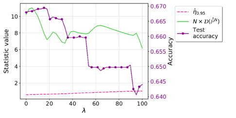
(a) Regularized logistics classifier in COMPAS

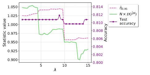
(b) SVM classifier in Drug dataset

Figure 1: Test statistics and accuracy of regularized classifiers on test data with a rejection threshold. The green line is the test statistics; the pink dashed line is the rejection threshold at the significance level $\alpha=0.05$; the purple line is the test accuracy; $\lambda$ denotes the regularization parameter, where larger $\lambda$ means stronger regularization power.

In the second experiment, we compare a fair algorithm proposed in Donini et al. (2018) with a naive SVM classifier (parametrized by the ridge regularization $\lambda$) in three datasets: Arrhythmia, COMPAS and Drug. We randomly split 70%-30% of the data as a train-test set and we replicate this procedure 1,000 times. We will test the fairness in terms of the equal opportunity and equalized odds criteria, and for the equal opportunity criteria, we will further show results using Welch’s test (Welch’s test is not applicable for multi-dimensional equalized odds criteria). Tables 1 and 2 show a rejection percentage of the naive SVM and the method in Donini et al. (2018) at the significance level $\alpha=0.05$ in those 1,000 replications using our test according to the equal opportunity and equalized odds criteria, respectively. Table 3 shows the test results using Welch’s test according to the equal opportunity criterion. Our test results demonstrate that the method in Donini et al. (2018) has a significantly lower rejection rate, which means it is substantially more fair than the naive method.

Table 1: Rejection percentage of the Naive SVM and the method in Donini et al. (2018) at the significance level $\alpha=0.05$ according to the equal opportunity criterion using our test.

	Arrhythmia	COMPAS	Drug
Naive SVM	68.4%	100%	30.1%
Donini et al. (2018)	11.6%	16.6%	21.6%

Table 2: Rejection percentage of the Naive SVM and the method in Donini et al. (2018) at the significance level $\alpha=0.05$ according to the equalized odds criterion using our test.

	Arrhythmia	COMPAS	Drug
Naive SVM	75.1%	100%	30.5%
Donini et al. (2018)	13.7%	21.7%	17.2%

Table 3: Rejection percentage of the Naive SVM and the method in Donini et al. (2018) at the significance level $\alpha=0.05$ according to the equal opportunity criterion using Welch’s test.

	Arrhythmia	COMPAS	Drug
Naive SVM	76.1%	100%	35.5%
Donini et al. (2018)	14.0%	16.1%	23.0%

More experiments are conducted in Appendix B.1 to empirically validate the convergence result in Theorem 1 and our proposed hypothesis test method.

Appendix A Proofs

We prove Theorems 1 and 2 under a more general assumption below.

Assumption 2^′ (Continuous conditional measure).

For the case where $\text{supp}(U)$ is potentially an infinite set, the cost function $c$ is decomposable as

$$c\left((x,u),(x^{\prime},u^{\prime})\right)=\bar{c}(x,x^{\prime})+\infty\cdot\|u-u^{\prime}\|,$$

and the following conditions are satisfied:

1. the moments $\mathbb{E}_{\mathbb{P}}\|U\|_{2}^{2}$, $\mathbb{E}_{\mathbb{P}}\|\phi(U,\mu)\|_{2}^{2}$ and $\mathbb{E}_{\mathbb{P}}\|\phi_{z}(U,\mu)\|_{2}$ are finite.

2. for $z$ such that $\|z-\mu\|_{2}<v,$ the derivative $\phi_{z}(\cdot)$ satisfies,

   $$\left\|\phi_{z}(u,z)-\phi_{z}(u,\mu)\right\|_{2}\leq M(u)\left\|z-\mu\right\|_{2},$$ (A.1)

   where $\mathbb{E}_{\mathbb{P}}[M(U)]<+\infty.$

3. The (regular) conditional probability measure $\nu_{t}$ of $\phi(U,\mu)|\Phi(X)=t$ converges in terms of the type $1$-Wasserstein distance as $t\rightarrow 0$: i.e., there exist a set $B\subset\mathbb{R}$ with $\mathbb{P}(\Phi(X)\in B)=1$ and $\varepsilon_{0}>0$ such that

   $$\lim_{t\rightarrow 0}W_{1}\left(\nu_{t},\nu_{0}\right)\mathbf{1}\{t\in B\}=0$$

   and $\sup_{t\in B}\mathbb{E}_{\mathbb{P}}[\|\phi(U,\mu)\|_{2}^{2+\epsilon_{0}}|\Phi(X)\mathcal{=}t]$ is finite, where type 1-Wasserstein distance $W_{1}(\cdot,\cdot)$ is $W_{c}(\cdot,\cdot)$ with the cost function being a metric.

Remark 1.

If $\text{supp}(U)$ is a finite set, and $U$ is completely dependent on $(X,Y)$, the simpler Assumption 2 is equivalent to Assumption 2^′.

Appendix A.1 Proofs of Section 3

Proof of Proposition 1.

Since the cost to move $U$ is $+\infty$, we have $\mathbb{E}_{\mathbb{Q}}[U]=\mathbb{E}_{\hat{\mathbb{P}}^{N}}[U]$. Then, consider any probability measure $\mathbb{Q}$ such that

$$\mathbb{E}_{\mathbb{Q}}[\mathcal{C}(X)\phi(U,\mathbb{E}_{\hat{\mathbb{P}}^{N}}[U])]=0,$$

and let $\pi$ be the optimal coupling between $\hat{\mathbb{P}}^{N}$ and $\mathbb{Q}$. Because $\hat{\mathbb{P}}^{N}$ is the empirical measure, the coupling $\pi$ can be written as $\pi=\frac{1}{N}\sum_{i\in[N]}\pi_{i}\otimes\delta_{(x_{i},u_{i})}$. For any value $\varepsilon>0$, construct now the measure

$$\mathbb{Q}^{\varepsilon}=\frac{1}{N}\sum_{i\in[N]}(1-p_{i})\delta_{(x_{i},u_{i})}+p_{i}\delta_{(x_{i}^{\varepsilon},u_{i})},$$ (A.2)

where the mass $p_{i}$ is set to

$$p_{i}=\int_{\mathbb{X}_{1-\mathcal{C}(x_{i})}}\pi_{i}(\mathrm{d}x)=\pi_{i}(\mathbb{X}_{1-\mathcal{C}(x_{i})})\in[0,1]\qquad\forall i\in[N]$$

and ${x}^{\varepsilon}_{i}$ is an $\varepsilon$-optimizer of the problem $\inf_{x^{\prime}\in\mathbb{X}_{1-\mathcal{C}(x)}}c(x_{i},x^{\prime})$. Then, it is easy to see that

$$\mathbb{E}_{\mathbb{Q}^{\varepsilon}}[\mathcal{C}(X)\phi(U,\mathbb{E}_{\hat{\mathbb{P}}^{N}}[U])]=\mathbb{E}_{\mathbb{Q}}[\mathcal{C}(X)\phi(U,\mathbb{E}_{\hat{\mathbb{P}}^{N}}[U])]=0$$

and that

$$\mathbb{E}_{\mathbb{Q}^{\varepsilon}}[\mathcal{C}(X)\phi(U,\mathbb{E}_{\hat{\mathbb{P}}^{N}}[U])]$$

$$=\frac{1}{N}\left(\displaystyle\sum_{i\in[N]}(1-p_{i})\mathcal{C}(x_{i})\phi(u_{i},\mathbb{E}_{\hat{\mathbb{P}}^{N}}[U])+p_{i}(1-\mathcal{C}(x_{i}))\phi(u_{i},\mathbb{E}_{\hat{\mathbb{P}}^{N}}[U])\right)$$

$$=\frac{1}{N}\left(\displaystyle\sum_{i\in[N]}(1-2\mathcal{C}(x_{i}))\phi(u_{i},\mathbb{E}_{\hat{\mathbb{P}}^{N}}[U])p_{i}+\sum_{i\in[N]}\mathcal{C}(x_{i})\phi(u_{i},\mathbb{E}_{\hat{\mathbb{P}}^{N}}[U])\right).$$

Since $d(x_{i})\leq\|x_{i}^{\varepsilon}-x_{i}\|\leq\|x-x_{i}\|+\varepsilon$ for any $x\in\mathbb{X}_{1-\mathcal{C}(x_{i})}$, this implies that $\frac{1}{N}\sum_{i\in[N]}p_{i}d(x_{i})\leq W(\mathbb{Q},\hat{\mathbb{P}}^{N})+\varepsilon$. Since $\varepsilon$ can be chosen arbitrarily, this implies that

$$\mathcal{P}(\hat{\mathbb{P}}^{N})\geq\left\{\begin{array}[]{cl}\min&\displaystyle\frac{1}{N}\sum_{i\in[N]}p_{i}d(x_{i})\\ \mathrm{s.t.}&p\in[0,1]^{N}\\ &\displaystyle\sum_{i\in[N]}(1-2\mathcal{C}(x_{i}))\phi(u_{i},\mathbb{E}_{\hat{\mathbb{P}}^{N}}[U])p_{i}=-\sum_{i\in[N]}\mathcal{C}(x_{i})\phi(u_{i},\mathbb{E}_{\hat{\mathbb{P}}^{N}}[U]).\end{array}\right.$$ (A.3)

On the other hand, for any $\{p_{i}\}_{i=1}^{N}$ satisfying the constraints in the linear programming (A.3), we can construct the measure $\mathbb{Q}^{\varepsilon}$ according to (A.2). Since $\mathbb{Q}^{\varepsilon}$ is a feasible solution of the primal problem (7), we have the other direction of the inequality.    

Proof of Proposition 2.

Case 1: $d(x_{i})<+\infty$ for $i\in[N]$. The primal problem has a feasible solution ($p_{i}=0$ if $\mathcal{C}(X)=0$; $p_{i}=1$, otherwise) and is bounded, thus it has an optimal solution and the strong duality holds. By the strong duality, we have

$$\mathcal{P}(\hat{\mathbb{P}}^{N})=\left\{\begin{array}[]{cl}\max&\displaystyle\frac{1}{N}\left\{\sum_{i\in[N]}\alpha^{i}+\gamma^{\top}\mathcal{C}(x_{i})\phi(u_{i},\mathbb{E}_{\hat{\mathbb{P}}^{N}}[U])\right\}\\ \mathrm{s.t.}&\alpha_{i}\leq 0\quad\forall i\in[N]\\ &\displaystyle\alpha_{i}-\left(1-2\mathcal{C}(x_{i})\right)\gamma^{\top}\phi(u_{i},\mathbb{E}_{\hat{\mathbb{P}}^{N}}[U])\leq d(x_{i})\quad\forall i\in[N].\end{array}\right.$$ (A.4)

Then, we have

$$\alpha_{i}=\left(d(x_{i})+\left(1-2\mathcal{C}(x_{i})\right)\gamma^{\top}\phi(u_{i},\mathbb{E}_{\hat{\mathbb{P}}^{N}}[U])\right)^{-},$$

which gives the desired results.

Case 2: $\exists i\in[N]$ such that $d(x_{i})=+\infty$. The primal problem is equivalent to

$$\mathcal{P}(\hat{\mathbb{P}}^{N})=\left\{\begin{array}[]{cl}\min&\displaystyle\frac{1}{N}\sum_{i\in[N]}p_{i}d(x_{i}),\\ \mathrm{s.t.}&p\in[0,1]^{N},\\ &p_{i}=0\text{ for }d(x_{i})=+\infty\\ &\displaystyle\sum_{i\in[N]}(1-2\mathcal{C}(x_{i}))\phi(u_{i},\mathbb{E}_{\hat{\mathbb{P}}^{N}}[U])p_{i}=-\displaystyle\sum_{i\in[N]}\mathcal{C}(x_{i})\phi(u_{i},\mathbb{E}_{\hat{\mathbb{P}}^{N}}[U]),\end{array}\right.$$ (A.5)

with the convention that if the problem is infeasible, the optimal value of the minimization problem is $+\infty$. We have the dual problem

$$\begin{array}[]{cl}\max&\displaystyle\frac{1}{N}\left\{\sum_{d(x_{i})<+\infty}\alpha^{i}+\gamma^{\top}\mathcal{C}(x_{i})\phi(u_{i},\mathbb{E}_{\hat{\mathbb{P}}^{N}}[U])\right\}\\ \mathrm{s.t.}&\alpha_{i}\leq 0\quad\text{ for }d(x_{i})<+\infty\\ &\displaystyle\alpha_{i}-\left(1-2\mathcal{C}(x_{i})\right)\gamma^{\top}\phi(u_{i},\mathbb{E}_{\hat{\mathbb{P}}^{N}}[U])\leq d(x_{i})\quad\text{ for }d(x_{i})<+\infty.\end{array}$$ (A.6)

Since the problem (A.6) is also feasible, if it is bounded, then the strong duality holds. If the problem (A.6) is unbounded, the primal problem (A.5) is infeasible, which means the primal and the dual both have optimal value $+\infty$. Finally, because

$$\left(d(x_{i})+\left(1-2\mathcal{C}(x_{i})\right)\gamma^{\top}\phi(u_{i},\mathbb{E}_{\hat{\mathbb{P}}^{N}}[U])\right)^{-}=0\text{ for }d(x_{i})=+\infty,$$

we have the optimal value of problem (A.6) equals to $\mathcal{D}(\hat{\mathbb{P}}^{N})$.    

Proof of Lemma 1.

Since $X_{C}\big{|}X_{D}=x$ has positive density in $\mathbb{R}^{d_{2}}$ for every $x\in\mathbb{D}$, we have $\theta_{C}^{\top}X_{C}\big{|}X_{D}=x$ has positive density in $\mathbb{R}$ for every $x\in\mathbb{D}$. Therefore, $\theta^{\top}X$ has a density

$$f_{\theta^{\top}X}(x)=\sum_{v\in\mathbb{D}}p_{v}f_{\theta_{C}^{\top}X_{C}\big{|}v}(x-\theta_{D}^{\top}v)>0,$$

where $p_{v}=\mathbb{P}\left(X_{D}=v\right)$ and $f_{\theta_{C}^{\top}X_{C}\big{|}v}(\cdot)$ denotes the conditional density of $\theta_{C}^{\top}X_{C}\big{|}X_{D}=x$.

Further, let $w=\ell^{-1}(\tau)$. For the cost function $\bar{c}(\cdot)$ given by (3a), we have by Hölder inequality

$$d(x)=\inf_{\theta^{\top}x^{\prime}=w}\|x-x^{\prime}\|=\|\theta\|^{-1}_{*}|\theta^{\top}x-w|.$$

Therefore, $\mathbb{P}_{\Phi}$ has a continuous density $f(\cdot)=\|\theta\|_{*}f_{\theta^{\top}X}(\|\theta\|_{*}\times\cdot+w)$ with $f(0)>0$.

For the cost function $\bar{c}(\cdot)$ given by (4), when $d(x)<\delta$, we have

$$d(x)=\inf_{\theta^{\top}x^{\prime}=w}\bar{c}(x,x^{\prime})=\inf_{x_{D}=x_{D}^{\prime},\theta_{C}^{\top}x^{\prime}=w-\theta_{D}^{\top}x_{D}}\bar{c}(x,x^{\prime})=\inf_{\theta_{C}^{\top}x^{\prime}=w-\theta_{D}^{\top}x_{D}}\|x_{C}-x_{C}^{\prime}\|=\|\theta_{C}\|^{-1}_{*}|\theta^{\top}x-w|.$$

The last equality is again due to Hölder inequality. Therefore, $\mathbb{P}_{\Phi}$ has a continuous density $f(\cdot)=\|\theta_{C}\|_{*}f_{\theta^{\top}X}(\|\theta_{C}\|_{*}\times\cdot+w)$ with $f(0)>0$, which completes the proof.    

Lemmas A2 and A3 are useful for the proof of Theorem 1, whose proofs are presented in Appendix A.3.

Lemma A2.

Suppose Assumption 2^′ is enforced. Then, we have

$$\sqrt{N}\left(\mathbb{E}_{\mathbb{\hat{P}}^{N}}\left[\phi\left(U,\mathbb{E}_{\mathbb{\hat{P}}^{N}}[U]\right)\mathcal{C}(X)\right]-\mathbb{E}_{\mathbb{P}}\left[\phi(U,\mu)\mathcal{C}(X)\right]\right)\Rightarrow\mathcal{N}(0,\mathrm{cov}\left(\mathbb{E}_{\mathbb{P}}\left[\phi_{z}(U,\mu)\mathcal{C}(X)\right]U+\phi(U,\mu)\mathcal{C}(X)\right)).$$

Lemma A3.

Suppose Assumption 1 and 2^′ are enforced. Then, we have

$$\sqrt{N}\mathbb{E}_{\mathbb{\hat{P}}^{N}}\left[\left(-\gamma^{\top}\phi\left(U,\mathbb{E}_{\mathbb{\hat{P}}^{N}}[U]\right)+\sqrt{N}d(X)\right)^{-}\mathcal{C}(X)\right]\overset{p}{\longrightarrow}-\frac{1}{2}f(0)\mathbb{E}_{\mathbb{P}}\left[\left.\left(\gamma^{\top}\phi\left(U,\mu\right)\right)^{2}\mathbb{I}\{\gamma^{\top}\phi\left(U,\mu\right)\geq 0\}\right|d(X\mathcal{)}=0\right],$$

uniformly over $\left\|\gamma\right\|_{2}\leq B.$

We are now ready to prove Theorem 1.

Proof of Theorem 1.

Recall that

$$\mathcal{D}(\mathbb{\hat{P}}^{N}) = \max_{\gamma\in\mathbb{R}^{m}}\frac{1}{N}\left\{\sum_{i\in[N]}\left(d(x_{i})+\left(1-2\mathcal{C}(x_{i})\right)\gamma^{\top}\phi(u_{i},\mathbb{E}_{\hat{\mathbb{P}}^{N}}[U])\right)^{-}+\gamma^{\top}\mathcal{C}(x_{i})\phi(u_{i},\mathbb{E}_{\hat{\mathbb{P}}^{N}}[U])\right\}$$

$$= \max_{\gamma\in\mathbb{R}^{m}}\left\{\frac{1}{N}\sum_{i\in[N]}\gamma^{\top}\mathcal{C}(x_{i})\phi(u_{i},\mathbb{E}_{\hat{\mathbb{P}}^{N}}[U])\right.+$$

$$\left.\frac{1}{N}\sum_{i\in[N]}\left(d(x_{i})-\gamma^{\top}\phi(u_{i},\mathbb{E}_{\hat{\mathbb{P}}^{N}}[U])\right)^{-}\mathcal{C}(x_{i})+\left(d(x_{i})+\gamma^{\top}\phi(u_{i},\mathbb{E}_{\hat{\mathbb{P}}^{N}}[U])\right)^{-}(1-\mathcal{C}(x_{i}))\right\}.$$

We first rescale $\gamma\leftarrow\gamma\sqrt{N}$ and thus

$$N\mathcal{D}(\mathbb{\hat{P}}^{N})$$

$$= \sqrt{N}\max_{\gamma\in\mathbb{R}^{m}}\left\{\gamma^{\top}\mathbb{E}_{\mathbb{\hat{P}}^{N}}\left[\phi\left(U,\mathbb{E}_{\mathbb{\hat{P}}^{N}}[U]\right)\mathcal{C}(X)\right]\right.+$$

$$\left.\mathbb{E}_{\mathbb{\hat{P}}^{N}}\left[\left(\sqrt{N}d(X)-\gamma^{\top}\phi(U,\mathbb{E}_{\hat{\mathbb{P}}^{N}}[U])\right)^{-}\mathcal{C}(X)+\left(\sqrt{N}d(X)+\gamma^{\top}\phi(U,\mathbb{E}_{\hat{\mathbb{P}}^{N}}[U])\right)^{-}(1-\mathcal{C}(X))\right]\right\}.$$

To ease the notation, we denote $\lambda_{i}=\phi\left(u_{i},\mathbb{E}_{\mathbb{\hat{P}}^{N}}[U]\right)$. By Lemma A3, we have

$$\frac{1}{\sqrt{N}}\sum_{i=1}^{N}\left(-\gamma^{\top}\lambda_{i}+N^{1/2}d(x_{i})\right)^{-}\mathcal{(}1-\mathcal{C}(x_{i}))$$

$$\overset{p}{\longrightarrow} -\frac{1}{2}f(0)\mathbb{E}_{\mathbb{P}}\left[\left.\left(\gamma^{\top}\phi\left(U,\mu\right)\right)^{2}\mathbb{I}\{\gamma^{\top}\phi\left(U,\mu\right)\geq 0\}\right|d(X\mathcal{)}=0\right]$$

$$= -\frac{1}{2}f(0)\mathbb{E}_{\mathbb{P}}\left[\left.\left(\gamma^{\top}\phi\left(U,\mu\right)\right)^{2}\mathbb{I}\{\gamma^{\top}\phi\left(U,\mu\right)\geq 0\}\right|d(X)=0\right],$$

and similarly, we have

$$\frac{1}{\sqrt{N}}\sum_{i=1}^{N}\left(\gamma^{\top}\lambda_{i}+N^{1/2}d(x_{i})\right)^{-}(1-\mathcal{C}(x_{i}))\overset{p}{\longrightarrow}-\frac{1}{2}f(0)\mathbb{E}_{\mathbb{P}}\left[\left.\left(\gamma^{\top}\phi\left(U,\mu\right)\right)^{2}\mathbb{I}\{\gamma^{\top}\phi\left(U,\mu\right)<0\}\right|d(X)=0\right].$$

Therefore, we have

$$\sqrt{N}\mathbb{E}_{\mathbb{\hat{P}}^{N}}\left[\left(\sqrt{N}d(X)-\gamma^{\top}\phi(U,\mathbb{E}_{\hat{\mathbb{P}}^{N}}[U])\right)^{-}\mathcal{C}(X)+\left(\sqrt{N}d(X)+\gamma^{\top}\phi(U,\mathbb{E}_{\hat{\mathbb{P}}^{N}}[U])\right)^{-}(1-\mathcal{C}(X))\right]$$

$$\overset{p}{\longrightarrow}-\frac{1}{2}f(0)\mathbb{E}_{\mathbb{P}}\left[\left.\left(\gamma^{\top}\phi\left(U,\mu\right)\right)^{2}\right|d(X)=0\right].$$

We denote

$$V_{N} = \sqrt{N}\mathbb{E}_{\mathbb{\hat{P}}^{N}}\left[\phi\left(U,\mathbb{E}_{\mathbb{\hat{P}}^{N}}[U]\right)\mathcal{C}(X)\right],\text{ and}$$

$$M_{N}(\gamma) = \frac{1}{\sqrt{N}}\sum_{i=1}^{N}\left[\left(-\gamma^{\top}\lambda_{i}+N^{1/2}d(x_{i})\right)^{-}\mathcal{C}(X)\}+\left(\gamma^{\top}\lambda_{i}+N^{1/2}d(x_{i})\right)^{-}(1-\mathcal{C}(X))\right]\text{ .}$$

To proceed, we rely on the following lemma.

Lemma A4.

Suppose Assumption 1 is enforced. Then, for every $\varepsilon>0,$ there exists $N_{0}>0$ and $b\in(0,\infty)$ such that for all $N\geq$ $N_{0}$,

$$\mathbb{P}\left(\sup_{\left\|\gamma\right\|_{2}>b}\left\{\gamma^{\top}V_{N}+M_{N}(\gamma)\right\}>0\right)\leq\varepsilon.$$

The proof of Lemma A4 is furnished in Appendix A.3. Notice that $\mathcal{D}(\hat{\mathbb{P}}^{N})\geq 0$ (choosing $\gamma=0),$ Lemma A4 implies that when $N\geq N_{0}$,

$$\mathbb{P}\left\{N\mathcal{D}(\hat{\mathbb{P}}^{N})=\sup_{\left\|\gamma\right\|_{2}\leq b}\left\{\gamma^{\top}V_{N}+M_{N}(\gamma)\right\}\right\}\geq 1-\varepsilon.$$

By Lemmas A2 and A3, we have

$$\sup_{\left\|\gamma\right\|_{2}\leq b}\left\{\gamma^{\top}V_{N}+M_{N}(\gamma)\right\} \Rightarrow \sup_{\left\|\gamma\right\|_{2}\leq b}\left\{\gamma^{\top}V-\frac{1}{2}f(0)\mathbb{E}\left[\left.\left(\gamma^{\top}\phi\left(U,\mu\right)\right)^{2}\right|d(X)=0\right]\right\}$$

$$= \sup_{\left\|\gamma\right\|_{2}\leq b}\left\{\gamma^{\top}V-\frac{1}{2}\gamma^{\top}S\gamma\right\},$$

where

$$S=f(0)\mathbb{E}_{\mathbb{P}}\left[\left.\phi\left(U,\mu\right)\phi\left(U,\mu\right)^{\top}\right|d(X)=0\right],$$

and $V$ is normally distributed with mean zero and covariance matrix

$$\mathrm{cov}\left(\mathbb{E}_{\mathbb{P}}\left[\phi_{z}(U,\mu)\mathcal{C}(X)\right]U+\phi(U,\mu)\mathcal{C}(X)\right).$$

By the arbitrariness of $\varepsilon,$ we have the desired result:

$$N\times\mathcal{D}(\hat{\mathbb{P}}^{N})\Rightarrow\sup_{\gamma}\left\{\gamma^{\top}V-\frac{1}{2}\gamma^{\top}S\gamma\right\}.$$

This completes the proof.    

Appendix A.2 Proofs of Section 4

The proofs of Propositions 4 and 5 are not presented because they follow the same lines as the proofs of Propositions 1 and 2.

Proof of Theorem 2.

Let ${\epsilon}^{\ast}=\mathbb{E}_{\mathbb{P}}\left[\mathcal{C}(X)\phi\left(U,\mathbb{E}_{\mathbb{P}}[U]\right)\right]$. By following the similar arguments with the proof of Theorem 1, we have

$$N\mathcal{D}_{\epsilon}(\mathbb{\hat{P}}^{N})$$

$$= N\sup_{\gamma\in\mathbb{R}_{+}^{m}}\left\{-\gamma^{\top}\epsilon+\frac{1}{N}\left\{\sum_{i\in[N]}(1-2\mathcal{C}(x_{i}))\phi(u_{i},\mathbb{E}_{\hat{\mathbb{P}}^{N}}[U])+\sum_{i\in[N]}\mathcal{C}(x_{i})\phi(u_{i},\mathbb{E}_{\hat{\mathbb{P}}^{N}}[U])\right\}\right\}$$

$$= \sqrt{N}\sup_{\gamma\in\mathbb{R}_{+}^{m}}\left\{\gamma^{\top}\left(\mathbb{E}_{\mathbb{\hat{P}}^{N}}\left[\phi\left(U,\mathbb{E}_{\mathbb{\hat{P}}^{N}}[U]\right)\mathcal{C}(X)\}-\epsilon\right]\right)\right.+$$

$$\left.\mathbb{E}_{\mathbb{\hat{P}}^{N}}\left[\left(-\gamma^{\top}\phi(U,\mathbb{E}_{\hat{\mathbb{P}}^{N}}[U])+\sqrt{N}d(X)\right)^{-}\mathcal{C}(X)+\left(\gamma^{\top}\phi(U,\mathbb{E}_{\hat{\mathbb{P}}^{N}}[U])+\sqrt{N}d(X)\right)^{-}\left(1-\mathcal{C}(X)\right)\right]\right\}$$

$$= \sup_{\gamma\in\mathbb{R}_{+}^{m}}\left\{\gamma^{\top}V_{N}+\sqrt{N}\gamma^{\top}\left(\epsilon^{\ast}-\epsilon\right)+M_{N}(\gamma)\right\}.$$

Similarly, we still have

$$\gamma^{\top}V_{N}+M_{N}(\gamma)\Rightarrow\gamma^{\top}V-\frac{1}{2}\gamma^{\top}S\gamma,$$

uniformly over $\left\{\gamma:\gamma\in\mathbb{R}^{m}_{+},\left\|\gamma\right\|_{2}\leq B\right\}$. Therefore, we must enforce $\gamma^{\top}\left(\epsilon^{\ast}-\epsilon\right)=0$ here. Then, we have

$$N\mathcal{D}_{\epsilon}(\mathbb{\hat{P}}^{N})\Rightarrow\max_{\gamma\in\mathbb{R}^{m}_{+},\gamma^{\top}\left(\epsilon^{\ast}-\epsilon\right)=0}\left\{\gamma^{\top}V-\frac{1}{2}\gamma^{\top}S\gamma\right\}\preceq\max_{\gamma\in\mathbb{R}_{+}^{m}}\left\{\gamma^{\top}V-\frac{1}{2}\gamma^{\top}S\gamma\right\}.$$

This completes the proof.    

Appendix A.3 Proofs of Technical Results

Proof of Lemma A2.

By adding and subtracting the term $\mathbb{E}_{\mathbb{\hat{P}}^{N}}\left[\phi(U,\mu)\mathcal{C}(X)\right]$, we find

$$\begin{array}[]{rl}&\mathbb{E}_{\mathbb{\hat{P}}^{N}}\left[\phi(U,\mathbb{E}_{\mathbb{\hat{P}}^{N}}[U])\mathcal{C}(X)\right]-\mathbb{E}_{\mathbb{P}}\left[\phi(U,\mu)\mathcal{C}(X)\right]\\ =&\mathbb{E}_{\mathbb{\hat{P}}^{N}}\left[\phi(U,\mathbb{E}_{\mathbb{\hat{P}}^{N}}[U])\mathcal{C}(X)-\phi(U,\mu)\mathcal{C}(X)\right]+\mathbb{E}_{\mathbb{\hat{P}}^{N}}\left[\phi(U,\mu)\mathcal{C}(X)\right]-\mathbb{E}_{\mathbb{P}}\left[\phi(U,\mu)\mathcal{C}(X)\right]\end{array}$$ (A.7)

Under Assumption 2^′ and the fundamental theorem of calculus, the first term in the right-hand side of (A.7) becomes

$$\mathbb{E}_{\mathbb{\hat{P}}^{N}}\left[\phi(U,\mathbb{E}_{\mathbb{\hat{P}}^{N}}[U])\mathcal{C}(X)-\phi(U,\mu)\mathcal{C}(X)\right]=\mathbb{E}_{\mathbb{\hat{P}}^{N}}\left[\int_{0}^{1}\phi_{z}\left(U,\mu+t\left(\mathbb{E}_{\mathbb{\hat{P}}^{N}}[U]-\mu\right)\right)\left(\mathbb{E}_{\mathbb{\hat{P}}^{N}}[U]-\mu\right)\mathcal{C}(X)\mathrm{d}t\right].$$

Thanks to Assumption 2^′, we have that

$$\left\|\mathbb{E}_{\mathbb{\hat{P}}^{N}}\left[\int_{0}^{1}\phi_{z}\left(U,\mu+t\left(\mathbb{E}_{\mathbb{\hat{P}}^{N}}[U]-\mu\right)\right)\left(\mathbb{E}_{\mathbb{\hat{P}}^{N}}[U]-\mu\right)\mathcal{C}(X)\mathrm{d}t\right]\right.$$

$$\left.\qquad-\mathbb{E}_{\mathbb{\hat{P}}^{N}}\left[\int_{0}^{1}\phi_{z}\left(U,\mu\right)\left(\mathbb{E}_{\mathbb{\hat{P}}^{N}}[\psi(U)]-\mu\right)\mathcal{C}(X)\mathrm{d}t\right]\right\|_{2}$$

$$\leq \frac{1}{2}\mathbb{E}_{\mathbb{\hat{P}}^{N}}\left[M(U)\right]\left\|\mathbb{E}_{\mathbb{\hat{P}}^{N}}[U]-\mu\right\|_{2}^{2},$$

whenever $\left\|\mathbb{E}_{\hat{\mathbb{P}}^{N}}[U]-\mu\right\|_{2}<\varepsilon_{\mu}$. Then, notice that we have

$$\lim_{N\rightarrow\infty}\frac{1}{2}\sqrt{N}\mathbb{E}_{\mathbb{\hat{P}}^{N}}\left[M(U)\right]\left\|\mathbb{E}_{\mathbb{\hat{P}}^{N}}[\psi(U)]-\mu\right\|_{2}^{2}=0\text{ almost surely,}$$ (A.8)

and

$$\mathbb{E}_{\mathbb{\hat{P}}^{N}}\left[\int_{0}^{1}\phi_{z}\left(U,\mu\right)\left(\mathbb{E}_{\mathbb{\hat{P}}^{N}}[U]-\mu\right)\mathcal{C}(X)\mathrm{d}t\right] = \mathbb{E}_{\mathbb{\hat{P}}^{N}}\left[\phi_{z}\left(U,\mu\right)\mathcal{C}(X)\right]\left(\mathbb{E}_{\mathbb{\hat{P}}^{N}}[U]-\mu\right)\}$$

$$= \left(\mathbb{E}_{\mathbb{P}}\left[\phi_{z}\left(U,\mu\right)\mathcal{C}(X)\right]+o_{p}\left(1\right)\right)\left(\mathbb{E}_{\mathbb{\hat{P}}^{N}}[\psi(U)]-\mu\right).$$

By multiplying $\sqrt{N}$ to both sides of equation (A.7), we have

$$\sqrt{N}\left(\mathbb{E}_{\mathbb{\hat{P}}^{N}}\left[\phi\left(U,\mathbb{E}_{\mathbb{\hat{P}}^{N}}[U]\right)\mathcal{C}(X)\right]-\mathbb{E}_{\mathbb{P}}\left[\phi(U,\mu)\mathcal{C}(X)\right]\right)$$

$$= \sqrt{N}\left(\mathbb{E}_{\mathbb{P}}\left[\phi_{z}\left(U,\mu\right)\mathcal{C}(X)\right]+o_{p}\left(1\right)\right)\left(\mathbb{E}_{\mathbb{\hat{P}}^{N}}[U]-\mu\right)+\mathbb{E}_{\mathbb{\hat{P}}^{N}}\left[\phi(U,\mu)\mathcal{C}(X)\right]-\mathbb{E}_{\mathbb{P}}\left[\phi(U,\mu)\mathcal{C}(X)\right]+o_{p}(1)$$

$$= \sqrt{N}\mathbb{E}_{\mathbb{\hat{P}}^{N}}\Big{[}\mathbb{E}_{\mathbb{P}}\big{[}\phi_{z}\left(U,\mu\right)\mathcal{C}(X)\big{]}\left(U-\mu\right)+\phi(U,\mu)\mathcal{C}(X)-\mathbb{E}_{\mathbb{P}}\big{[}\phi(U,\mu)\mathcal{C}(X)\big{]}\Big{]}+o_{p}(1)$$

$$\Rightarrow \mathcal{N}(0,\Sigma),$$

where $\Sigma$ is the covariance matrix of $\mathbb{E}_{\mathbb{P}}\left[\phi_{z}(U,\mu)\mathcal{C}(X)\right]U+\phi(U,\mu)\mathcal{C}(X)$, namely

$$\Sigma=\mathrm{cov}\left(\mathbb{E}_{\mathbb{P}}\left[\phi_{z}(U,\mu)\mathcal{C}(X)\right]U+\phi(U,\mu)\mathcal{C}(X)\right).$$

This completes the proof.    

Proof of Lemma A3.

Step 1: we first show

$$\sqrt{N}\mathbb{E}_{\mathbb{\hat{P}}^{N}}\left[\left(-\gamma^{\top}\phi\left(U,\mathbb{E}_{\mathbb{\hat{P}}^{N}}[U]\right)+\sqrt{N}d(X)\right)^{-}\mathcal{C}(X)\right]-\sqrt{N}\mathbb{E}_{\mathbb{\hat{P}}^{N}}\left[\left(-\gamma^{\top}\phi\left(U,\mu\right)+\sqrt{N}d(X)\right)^{-}\mathcal{C}(X)\right]\overset{p}{\longrightarrow}0,$$

uniformly over $\left\|\gamma\right\|_{2}\leq B.$ When $\left\|\mathbb{E}_{\mathbb{\hat{P}}^{N}}[U]-\mu\right\|_{2}<\varepsilon_{\mu},$ we have

$$\sqrt{N}\mathbb{E}_{\mathbb{\hat{P}}^{N}}\left[\left(-\gamma^{\top}\phi\left(U,\mathbb{E}_{\mathbb{\hat{P}}^{N}}[U]\right)+\sqrt{N}d(X)\right)^{-}\mathcal{C}(X)\right]-\sqrt{N}\mathbb{E}_{\mathbb{\hat{P}}^{N}}\left[\left(-\gamma^{\top}\phi\left(U,\mu\right)+\sqrt{N}d(X)\right)^{-}\mathcal{C}(X)\right]$$

$$\leq N^{-1/2}\left\|\gamma\right\|_{2}\sum_{i=1}^{N}\left[\left\|\phi\left(u_{i},\mathbb{E}_{\mathbb{\hat{P}}^{N}}[\psi(U)]\right)-\phi\left(u_{i},\mu\right)\right\|_{2}\mathbb{I\{}\mathcal{E}_{i}\}\right],$$

where the events $\mathcal{E}_{i}$ are defined by

$$\mathcal{E}_{i}=\mathbb{\{}\left\|\gamma\right\|_{2}\left(\left\|\phi\left(u_{i},\mu\right)\right\|_{2}+\left(\left\|\phi_{z}\left(u_{i},\mu\right)\right\|_{2}+M(u_{i})\varepsilon_{\mu}\right)\varepsilon_{\mu}\right){\geq}\sqrt{N}d(x_{i})\}.$$

By a similar derivation with the proof of Lemma A2, we have

$$N^{-1/2}\left\|\gamma\right\|_{2}\sum_{i=1}^{N}\left[\left\|\phi\left(u_{i},\mathbb{E}_{\mathbb{\hat{P}}^{N}}[U]\right)-\phi\left(u_{i},\mu\right)\right\|_{2}^{-}\mathbb{I\{}\mathcal{E}_{i}\}\right]$$

$$= \frac{\left\|\gamma\right\|_{2}}{\sqrt{N}}\sum_{i=1}^{N}\left[\int_{0}^{1}\left(\phi_{z}\left(u_{i},\mu+t\left(\mathbb{E}_{\mathbb{\hat{P}}^{N}}[U]-\mu\right)\right)\left(\mathbb{E}_{\mathbb{\hat{P}}^{N}}[U]-\mu\right)\mathrm{d}t\right)\mathbb{I\{}\mathcal{E}_{i}\}\right]$$

$$\leq \left\|\gamma\right\|_{2}\sqrt{N}\left(\mathbb{E}_{\mathbb{\hat{P}}^{N}}[U]-\mu\right)\mathbb{E}_{\mathbb{\hat{P}}^{N}}\left[\phi_{z}\left(U,\mu\right)\mathbb{I}\{\mathcal{E}_{i}\}\right]+\frac{1}{2}\left\|\gamma\right\|_{2}\sqrt{N}\mathbb{E}_{\mathbb{\hat{P}}^{N}}[M(U)]\left\|\mathbb{E}_{\mathbb{\hat{P}}^{N}}[U]-\mu\right\|_{2}^{2}.$$

Since $\mathbb{I}\{\mathcal{E}_{i}\}\rightarrow 0$ almost surely and $\mathbb{E}_{\mathbb{P}}[\phi_{z}(U,\mu)]<+\infty,$ we have

$$\left\|\gamma\right\|_{2}\sqrt{N}\left(\mathbb{E}_{\mathbb{\hat{P}}^{N}}[U]-\mu\right)\mathbb{E}_{\mathbb{\hat{P}}^{N}}\left[\phi_{z}\left(U,\mu\right)\mathbb{I}\{\mathcal{E}_{i}\}\right]\overset{p}{\longrightarrow}0,$$

uniformly over $\left\|\gamma\right\|_{2}\leq B.$ By combining

$$\frac{1}{2}\left\|\gamma\right\|_{2}\sqrt{N}\mathbb{E}_{\mathbb{\hat{P}}^{N}}[M(U)]\left\|\mathbb{E}_{\mathbb{\hat{P}}^{N}}[U]-\mu\right\|_{2}^{2}\rightarrow 0\text{ almost surely,}$$

uniformly over $\left\|\gamma\right\|_{2}\leq B,$ we finish step 1.

Step 2: We claim that

$$\sqrt{N}\mathbb{E}_{\mathbb{P}}\left[\left(-\gamma^{\top}\phi\left(U,\mu\right)+\sqrt{N}d(X)\right)^{-}\mathcal{C}(X)\right]\longrightarrow-\frac{1}{2}f(0)\mathbb{E}\left[\left.\left(\gamma^{\top}\phi\left(U,\mu\right)\right)^{2}\mathbb{I}\{\gamma^{\top}\phi\left(U,\mu\right)\geq 0\}\right|d(X)=0\right].$$

Notice that for any $c>0$, we have

$$\sqrt{N}\mathbb{E}_{\mathbb{P}}\left[\left(-\gamma^{\top}\phi\left(U,\mu\right)+\sqrt{N}d(X)\right)^{-}\mathcal{C}(X)\right]$$ (A.10)

$$= \sqrt{N}\int_{0}^{+\infty}\mathbb{E}_{\mathbb{P}}\left[\left.\left(-\gamma^{\top}\phi\left(U,\mu\right)+\sqrt{N}d(X)\right)^{-}\right|d(X)\left(2\mathcal{C}(X)-1\right)=t\right]\mathrm{d}\mathbb{P}_{\Phi}(t).$$

$$= \sqrt{N}\int_{0}^{c/\sqrt{N}}\mathbb{E}_{\mathbb{P}}\left[\left.\left(-\gamma^{\top}\phi\left(U,\mu\right)+\sqrt{N}d(X)\right)^{-}\right|\Phi(X)=t\right]\mathrm{d}\mathbb{P}_{\Phi}(t)$$

$$+\sqrt{N}\int_{c/\sqrt{N}}^{+\infty}\mathbb{E}_{\mathbb{P}}\left[\left.\left(-\gamma^{\top}\phi\left(U,\mu\right)+\sqrt{N}d(X)\right)^{-}\right|\Phi(X)=t\right]\mathrm{d}\mathbb{P}_{\Phi}(t)$$

We first analyze the first term in (A.10). By Assumption 1.a), when $N$ is sufficient large such that $c/\sqrt{N}<v$, we have

$$\sqrt{N}\int_{0}^{c/\sqrt{N}}\mathbb{E}_{\mathbb{P}}\left[\left.\left(-\gamma^{\top}\phi\left(U,\mu\right)+\sqrt{N}d(X)\right)^{-}\right|\Phi(X)=t\right]\mathrm{d}\mathbb{P}_{\Phi}(t)$$

$$= \sqrt{N}\int_{0}^{c/\sqrt{N}}\mathbb{E}_{\mathbb{P}}\left[\left.\left(-\gamma^{\top}\phi\left(U,\mu\right)+\sqrt{N}d(X)\right)^{-}\right|\Phi(X)=t\right]f(t)\mathrm{d}t.$$

By changing of the variable $s=\sqrt{N}t$ , we have

$$\sqrt{N}\int_{0}^{c/\sqrt{N}}\mathbb{E}_{\mathbb{P}}\left[\left.\left(-\gamma^{\top}\phi\left(U,\mu\right)+\sqrt{N}d_{\mathbb{B}}(X)\right)^{-}\right|\Phi(X)=t\right]f(t)\mathrm{d}t$$

$$= \int_{0}^{c}\mathbb{E}_{\mathbb{P}}\left[\left.\left(-\gamma^{\top}\phi\left(U,\mu\right)+s\right)^{-}\right|\Phi(X)=N^{-1/2}s\right]f(N^{-1/2}s)\mathrm{d}s$$

By Assumption 1.c), we have for any $\varepsilon>0,$ any $0<c<+\infty,$ there exists $N_{0},$ such that for $N>N_{0}$ and $s\leq c$,

$$\left|\mathbb{E}_{\mathbb{P}}\left[\left.\left(-\gamma^{\top}\phi\left(U,\mu\right)+s\right)^{-}\right|\Phi(X)=N^{-1/2}s\right]-\mathbb{E}_{\mathbb{P}}\left[\left.\left(-\gamma^{\top}\phi\left(U,\mu\right)+s\right)^{-}\right|\Phi(X)=0\right]\right|$$

$$\leq \left\|\gamma\right\|_{\ast}\left\|\mathbb{E}_{\mathbb{P}}\left[\left.\phi\left(U,\mu\right)\right|\Phi(X)=N^{-1/2}s\right]-\mathbb{E}_{\mathbb{P}}\left[\left.\phi\left(U,\mu\right)\right|\Phi(X)=0\right]\right\|$$

$$\leq \left\|\gamma\right\|_{\ast}W_{1}\left(\left.\phi\left(U,\mu\right)\right|\Phi(X)=N^{-1/2}s,\left.\phi\left(U,\mu\right)\right|\Phi(X)=0\right)\leq\varepsilon.$$

Therefore, by taking $\varepsilon\downarrow 0,$ we have

$$\left|\int_{0}^{c}\mathbb{E}_{\mathbb{P}}\left[\left.\left(-\gamma^{\top}\phi\left(U,\mu\right)+s\right)^{-}\mathbb{I\{}h\left({X}\right){\geq}\tau\}\right|\Phi(X)=N^{-1/2}s\right]f(N^{-1/2}s)\mathrm{d}s\right.$$

$$\left.-\int_{0}^{c}\mathbb{E}_{\mathbb{P}}\left[\left.\left(-\gamma^{\top}\phi\left(U,\mu\right)+s\right)^{-}\mathbb{I\{}h\left({X}\right){\geq}\tau\}\right|\Phi(X)=0\right]f(N^{-1/2}s)\mathrm{d}s\right|\overset{p}{\longrightarrow}0.$$

Then, the basic algebra and the mean value theorem for integrals give us

$$\int_{0}^{c}\mathbb{E}_{\mathbb{P}}\left[\left.\left(-\gamma^{\top}\phi\left(U,\mu\right)+s\right)^{-}\right|\Phi(X)=0\right]f(N^{-1/2}s)\mathrm{d}s$$

$$= \int_{0}^{c}\mathbb{E}_{\mathbb{P}}\left[\left.\left(-\gamma^{\top}\phi\left(U,\mu\right)+s\right)^{-}\right|d(X)=0\right]f(N^{-1/2}s)\mathrm{d}s$$

$$= f(\xi)\mathbb{E}_{\mathbb{P}}\left[\int_{0}^{c}\left(\left.\left(-\gamma^{\top}\phi\left(U,\mu\right)+s\right)^{-}\right|d(X)=0\right)\mathrm{d}s\right]$$

$$= f(\xi)\mathbb{E}_{\mathbb{P}}\left[\int_{0}^{\min(c,\gamma^{\top}\phi\left(U,\mu\right)|\Phi(X)=0)}\left(\left.\left(-\gamma^{\top}\phi\left(U,\mu\right)+s\right)\mathbb{I}\{\gamma^{\top}\phi\left(U,\mu\right)\geq 0\}\right|d(X)=0\right)\mathrm{d}s\right]$$

$$\rightarrow -\frac{1}{2}f(0)\mathbb{E}_{\mathbb{P}}\left[\min\{c,\gamma^{\top}\phi\left(U,\mu\right)\}\left(\gamma^{\top}\phi\left(U,\mu\right)+\left(\gamma^{\top}\phi\left(U,\mu\right)-c\right)^{+}\right)\mathbb{I}\{\gamma^{\top}\phi\left(U,\mu\right)\geq 0\}\big{|}d(X)=0\right],$$ (A.11)

where $\xi\in[0,N^{-1/2}c]$ and $(x)^{+}=\max\{x,0\}$.

We then deal with the second term in (A.10). Let

$$M_{\gamma}=\operatorname*{ess\,sup}_{t\geq 0}\mathbb{E}_{\mathbb{P}}\left[\left|\gamma^{\top}\phi\left(U,\mu\right)\right|^{2+\epsilon_{0}}|\Phi(X)\mathcal{=}t\right].$$

For any $c\geq 0,$ we have

$$\sqrt{N}\int_{c/\sqrt{N}}^{+\infty}\mathbb{E}_{\mathbb{P}}\left[\left.\left(-\gamma^{\top}\phi\left(U,\mu\right)+\sqrt{N}t\right)^{-}\right|\Phi(X)=t\right]\mathrm{d}\mathbb{P}_{\Phi}(t)$$

$$\geq -\sqrt{N}\int_{c/\sqrt{N}}^{+\infty}\mathbb{E}_{\mathbb{P}}\left[\gamma^{\top}\phi\left(U,\mu\right)\mathbb{I}\{\left.\gamma^{\top}\phi\left(U,\mu\right)\geq\sqrt{N}t\right|\Phi(X)=t\right]\mathrm{d}\mathbb{P}_{\Phi}(t)$$

$$\geq -\sqrt{N}\int_{c/\sqrt{N}}^{+\infty}\left(\frac{1}{\sqrt{N}t}\right)^{1+\epsilon_{0}}\mathbb{E}_{\mathbb{P}}\left[\left(\gamma^{\top}\phi\left(U,\mu\right)\right)^{2+\epsilon_{0}}\mathbb{I}\{\left.\gamma^{\top}\phi\left(U,\mu\right)\geq\sqrt{N}t\right|\Phi(X)=t\right]\mathrm{d}\mathbb{P}_{\Phi}(t)$$

$$\geq -\left(\sqrt{N}\right)^{-\epsilon_{0}}\int_{c/\sqrt{N}}^{+\infty}\frac{1}{t^{1+\epsilon_{0}}}\mathbb{E}_{\mathbb{P}}[\left|\gamma^{\top}\phi\left(U,\mu\right)\right|^{2+\epsilon_{0}}|\Phi(X)=t]\mathrm{d}\mathbb{P}_{\Phi}(t)$$

$$\geq -\left(\sqrt{N}\right)^{-\epsilon_{0}}M_{\gamma}\int_{c/\sqrt{N}}^{+\infty}\frac{1}{t^{1+\epsilon_{0}}}\mathrm{d}\mathbb{P}_{\Phi}(t).$$

We pick $\varepsilon>0$ such that $\mathbb{P}_{\Phi}\left(\cdot\right)$ has density in $[0,\varepsilon].$ Then, we have

$$\left(\sqrt{N}\right)^{-\epsilon_{0}}M_{\gamma}\int_{c/\sqrt{N}}^{+\infty}\frac{1}{t^{1+\epsilon_{0}}}f(t)\mathrm{d}t$$

$$= M_{\gamma}\left(\sqrt{N}\right)^{-\epsilon_{0}}\left(\int_{\varepsilon}^{+\infty}\frac{1}{t^{1+\epsilon_{0}}}f(t)\mathrm{d}\mathbb{P}_{\Phi}(t)+\int_{c/\sqrt{N}}^{\varepsilon}\frac{1}{t^{1+\epsilon_{0}}}f(t)\mathrm{d}t\right)$$

$$\leq M_{\gamma}\left(\left(\sqrt{N}\right)^{-\epsilon_{0}}\frac{1}{\varepsilon^{1+\epsilon_{0}}}+\frac{1}{\epsilon_{0}}\left(\sqrt{N}\right)^{-\epsilon_{0}}\left(\sqrt{N}/c\right)^{\epsilon_{0}}f(\xi)\right)$$

$$= M_{\gamma}\left(\left(\sqrt{N}\right)^{-\epsilon_{0}}\frac{1}{\varepsilon^{1+\epsilon_{0}}}+\frac{1}{c^{\epsilon_{0}}\epsilon_{0}}f(\xi)\right),$$

where $\xi\in(c/\sqrt{N},\varepsilon).\$ By taking $\varepsilon\downarrow 0,$ we have

$$\liminf_{N\rightarrow+\infty}\sqrt{N}\int_{c/\sqrt{N}}^{+\infty}\mathbb{E}_{\mathbb{P}}\left[\left.\left(-\gamma^{\top}\phi\left(U,\mu\right)+\sqrt{N}t\right)^{-}\right|\Phi(X)=t\right]\mathrm{d}\mathbb{P}_{\Phi}(t)\geq-\frac{M_{\gamma}f(0)}{c^{\epsilon_{0}}\epsilon_{0}}.$$

Finally, by taking $c\uparrow+\infty,$ we conclude step 2.

Step 3: We then apply weak law of triangular arrays Durrett (2019, Theorem 2.2.11). We need to check

$$N\times\left[\mathbb{P}\left(-\left(-\gamma^{\top}\phi\left(U,\mathbb{\mu}\right)+\sqrt{N}d(X)\right)\mathcal{C}(X)>\sqrt{N}\right)\right]\rightarrow 0,\text{ and}$$ (A.12a)

$$\mathbb{E}\left[\left(\left(-\gamma^{\top}\phi\left(U,\mu\right)+\sqrt{N}d(X)\right)^{-}\right)^{2}\mathcal{C}(X)\right]\rightarrow 0.$$ (A.12b)

For condition (A.12a), we have

$$N\mathbb{P}\left(-\left(-\gamma^{\top}\phi\left(U,\mu\right)+\sqrt{N}d(x_{i})\right)^{-}\mathcal{C}(X)>\sqrt{N}\right)$$

$$\leq N\mathbb{P}\left(\gamma^{\top}\phi\left(U,\mu\right)\geq\sqrt{N}\right)$$

$$\leq \frac{\mathbb{E}\left[\left(\gamma^{\top}\phi\left(U,\mathbb{\mu}\right)\right)^{2+\epsilon_{0}}\right]}{\left(\sqrt{N}\right)^{\epsilon_{0}}}\leq\frac{M_{\gamma}}{\left(\sqrt{N}\right)^{\epsilon_{0}}}\rightarrow 0.$$

For condition (A.12b), we have

$$\mathbb{E}\left[\left(\left(-\gamma^{\top}\phi\left(U,\mu\right)+\sqrt{N}d(X)\right)^{-}\right)^{2}\mathcal{C}(X)\right]$$

$$\leq \mathbb{E}\left[\left(\gamma^{\top}\phi\left(U,\mu\right)\right)^{2}\mathbb{I\{}\gamma^{\top}\phi\left(U,\mu\right){\geq}\sqrt{N}d(X)\}\right]$$

$$= \int_{0}^{+\infty}\mathbb{E}_{\mathbb{P}}\left[\left(\gamma^{\top}\phi\left(U,\mu\right)\right)^{2}\left.\mathbb{I}\left\{\gamma^{\top}\phi\left(U,\mu\right)\geq\sqrt{N}t\right\}\right|\Phi(X)=t\right]\mathrm{d}\mathbb{P}_{\Phi}(t).$$

We pick $\varepsilon>0$ such that $\mathbb{P}_{\Phi}\left(\cdot\right)$ has density in $[0,\varepsilon].$ Then, we have

$$\int_{0}^{+\infty}\mathbb{E}_{\mathbb{P}}\left[\left(\gamma^{\top}\phi\left(U,\mu\right)\right)^{2}\left.\mathbb{I}\left\{\gamma^{\top}\phi\left(U,\mu\right)\geq\sqrt{N}t\right\}\right|\Phi(X)=t\right]\mathrm{d}\mathbb{P}_{\Phi}(t)$$ (A.14)

$$= \int_{0}^{\varepsilon}\mathbb{E}_{\mathbb{P}}\left[\left(\gamma^{\top}\phi\left(U,\mu\right)\right)^{2}\left.\mathbb{I}\left\{\gamma^{\top}\phi\left(U,\mu\right)\geq\sqrt{N}t\right\}\right|\Phi(X)=t\right]f(t)\mathrm{d}t$$

$$+\int_{\varepsilon}^{+\infty}\mathbb{E}_{\mathbb{P}}\left[\left(\gamma^{\top}\phi\left(U,\mu\right)\right)^{2}\left.\mathbb{I}\left\{\gamma^{\top}\phi\left(U,\mu\right)\geq\sqrt{N}t\right\}\right|\Phi(X)=t\right]\mathrm{d}\mathbb{P}_{\Phi}(t).$$

For the first term (A.14), we have

$$\int_{0}^{\varepsilon}\mathbb{E}_{\mathbb{P}}\left[\left(\gamma^{\top}\phi\left(U,\mu\right)\right)^{2}\mathbb{I}\{\left.\gamma^{\top}\phi\left(U,\mu\right)\geq\sqrt{N}t\right|\Phi(X)=t\right]f(t)\mathrm{d}t\leq M_{\gamma}^{2/\left(2+\epsilon_{0}\right)}\varepsilon f(\xi),$$

where $\xi\in[0,\varepsilon].$ For the second term (A.14) we have

$$\int_{\varepsilon}^{+\infty}\mathbb{E}_{\mathbb{P}}\left[\left(\gamma^{\top}\phi\left(U,\mu\right)\right)^{2}\mathbb{I}\{\left.\gamma^{\top}\phi\left(U,\mu\right)\geq\sqrt{N}t\right|\Phi(X)=t\right]\mathrm{d}\mathbb{P}_{\Phi}(t)$$

$$\leq \int_{\varepsilon}^{+\infty}\frac{\mathbb{E}_{\mathbb{P}}\left[\left(\gamma^{\top}\phi\left(U,\mu\right)\right)^{2+\epsilon_{0}}\Phi(X)=t\right]}{\left(\sqrt{N}t\right)^{\epsilon_{0}}}\mathrm{d}\mathbb{P}_{\Phi}(t)$$

$$\leq \frac{M_{0}}{\left(\sqrt{N}\varepsilon\right)^{\epsilon_{0}}}\rightarrow 0.$$

By taking $\varepsilon\downarrow 0,$ we have

$$\int_{0}^{+\infty}\mathbb{E}_{\mathbb{P}}\left[\left(\gamma^{\top}\phi\left(U,\mu\right)\right)^{2}\mathbb{I}\{\left.\gamma^{\top}\phi\left(U,\mu\right)\geq\sqrt{N}t\right|\Phi(X)=t\right]\mathrm{d}\mathbb{P}_{\Phi}(t)\rightarrow 0.$$

We then apply Durrett (2019, Theorem 2.2.11) to obtain the weak law for each $\gamma.$

Step 4: We establish the Lipschitz continuity of

$$\sqrt{N}\mathbb{E}_{\mathbb{P}}\left[\left(-\gamma^{\top}\phi\left(U,\mathbb{\mu}\right)+\sqrt{N}d(X)\right)^{-}\mathcal{C}(X)\right]$$

for $\left\|\gamma\right\|_{2}\leq B,$ which ensures the tightness. For any $\gamma_{1},\gamma_{2}$ satisfying $\left\|\gamma_{1}\right\|_{2}\leq B$ and $\left\|\gamma_{2}\right\|_{2}\leq B,$ we have

$$\sqrt{N}\left|\mathbb{E}_{\mathbb{P}}\left[\left(-\gamma_{1}^{\top}\phi\left(U,\mu\right)+\sqrt{N}d(X)\right)^{-}\mathcal{C}(X)\right]\right.$$

$$- \left.\mathbb{E}_{\mathbb{P}}\left[\left(-\gamma_{2}^{\top}\phi\left(U,\mu\right)+\sqrt{N}d(X)\right)^{-}\mathcal{C}(X)\}\right]\right|$$

$$\leq \sqrt{N}\left\|\gamma_{1}-\gamma_{2}\right\|_{2}\left\|\phi\left(U,\mu\right)\right\|_{2}\mathcal{C}(X)\mathbb{I}\left\{B\left\|\phi\left(U,\mathbb{\mu}\right)\right\|_{2}\geq\sqrt{N}d(X)\right\}.$$

By following similar lines with steps 2 and 3, we have

$$\sqrt{N}\mathbb{E}_{\mathbb{\hat{P}}^{N}}\left[\left\|\phi\left(U,\mu\right)\right\|_{2}\mathcal{C}(X)\mathbb{I}\left\{B\left\|\phi\left(U,\mu\right)\right\|_{2}\geq\sqrt{N}d(X)\right\}\right]\overset{p}{\longrightarrow}f(0)\mathbb{E}_{\mathbb{P}}\left[\left.\left\|\phi\left(U,\mu\right)\right\|_{2}^{2}\right|d(X\mathcal{)}=0\right].$$

Then, by Billingsley (2013, Theorem 7.5), we have the desired uniform convergence result.    

Proof of Lemma A4.

Due to $\mathbb{E}\left[\left.\phi\left(U,\mu\right)\phi\left(U,\mu\right)^{\top}\right|d(X)=0\right]\succ 0$, there exists $\delta>0$ and $c_{0}\in(0,+\infty)$ such that

$$\inf_{\left\|\gamma\right\|_{2}=1}\mathbb{E}\left[\min\left\{c_{0},\gamma^{\top}\phi\left(U,\mu\right)\right\}\left|\gamma^{\top}\phi\left(U,\mu\right)\right|\right]>\delta.$$

for all $\left\|\gamma\right\|_{2}=1.$ And

$$\inf_{\left\|\gamma\right\|_{2}=1}\mathbb{E}\left|\gamma^{\top}\phi\left(U,\mu\right)\right|>0,$$

since the unit circle is compact. Let $\delta=\inf_{\left\|\gamma\right\|_{2}=1}\mathbb{E}\left|\gamma^{\top}\phi\left(U,\mathbb{\mu}\right)\right|.$ For any $\varepsilon>0,$ there exists $N_{1}>0$ and $b^{\prime}<+\infty,$ such that

$$\mathbb{P}(\left\|V_{N}\right\|_{2}\geq b^{\prime})<\varepsilon/2,$$

for any $N>N_{0}.$ Recalling Lemma A3 and equation (A.11), there exists $N_{0}>N_{1}$ such that

$$\mathbb{P}\left(\exists\gamma:\left\|\gamma\right\|_{2}=b\text{ such that }M_{N}(\gamma)\geq-\frac{1}{4}\mathbb{E}\left[\min\left\{bc_{0},\left|\gamma^{\top}\phi\left(U,\mu\right)\right|\right\}\left|\gamma^{\top}\phi\left(U,\mu\right)\right|\right]\right)<\varepsilon/2$$

for any $N>N_{0}$. Then, we have

$$\inf_{\left\|\gamma\right\|_{2}=b}\mathbb{E}\left[\min\left\{bc_{0},\left|\gamma^{\top}\phi\left(U,\mu\right)\right|\right\}\left|\gamma^{\top}\phi\left(U,\mu\right)\right|\right]$$

$$\geq b^{2}\inf_{\left\|\gamma\right\|_{2}=1}\mathbb{E}\left[\min\left\{c_{0},\left|\gamma^{\top}\phi\left(U,\mu\right)\right|\right\}\left|\gamma^{\top}\phi\left(U,\mu\right)\right|\right]>b^{2}\delta.$$

Let $b=4b^{\prime}/\delta.$ We have

$$\mathbb{P}\left(\sup_{\left\|\gamma\right\|_{2}=b\text{ }}M_{N}(\gamma)\geq-bb^{\prime}\right)<\varepsilon/2.$$ (A.15)

Notice that for any $\left\|\gamma\right\|_{2}>b,$

$$M_{N}(\gamma)\leq\frac{\left\|\gamma\right\|_{2}}{b}M_{N}\left(\frac{b}{\left\|\gamma\right\|_{2}}\gamma\right)\leq\frac{\left\|\gamma\right\|_{2}}{b}\sup_{\left\|\gamma\right\|_{2}=b\text{ }}M_{N}(\gamma).$$ (A.16)

By combining inequalities (A.15) and (A.16), we have

$$\mathbb{P}\left(\exists\gamma:\left\|\gamma\right\|_{2}>b,\text{ such that }M_{N}(\gamma)\geq-\left\|\gamma\right\|_{2}b^{\prime}\right)<\varepsilon/2.$$

Therefore,

$$\mathbb{P}\left(\sup_{\left\|\gamma\right\|_{2}>b}\left\{\gamma^{\top}V_{N}+M_{N}(\gamma)\right\}>0\right)$$

$$\leq \mathbb{P}\left(\sup_{\left\|\gamma\right\|_{2}>b}\left\{\left\|\gamma\right\|_{2}\left\|V_{N}\right\|_{2}+M_{N}(\gamma)\right\}>0\right)$$

$$\leq \mathbb{P}(\left\|V_{N}\right\|_{2}\geq b^{\prime})+\mathbb{P}\left(\exists\gamma:\left\|\gamma\right\|_{2}>b,\text{ such that }M_{N}(\gamma)\geq-\left\|\gamma\right\|_{2}b^{\prime}\right)$$

$$\leq \varepsilon.$$

This completes the proof.    

Appendix B Additional Details for Numerical Experiments

Appendix B.1 Validation of the Hypothesis Test

In this section, we empirically validate the convergence result in Theorem 1 and our proposed hypothesis test method. we use a simple logistic classifier in the form

$$\mathcal{C}(x)=\mathbb{I}\left\{\frac{1}{1+\exp\left(-\theta^{\top}x\right)}\geq\tau\right\}.$$

Then, the decision boundary is $\left\{x:\theta^{\top}x=-\log\left(\frac{1}{\tau}-1\right)\right\}.$ We denote $w=-\log\left(\frac{1}{\tau}-1\right).$ Then, we borrowed the example in Taskesen et al. (2021). Let

$$p_{11}=0.4,p_{01}=0.1,p_{10}=0.4,p_{00}=0.1.$$

Moreover, conditioning on $(A,Y)$, the feature $X$ follows a Gaussian distribution of the form

$$X|A=1,Y=1\sim \mathcal{N}([6,0],[3.5,0;0,5]),$$

$$X|A=0,Y=1\sim \mathcal{N}([-2,0],[5,0;0,5]),$$

$$X|A=1,Y=0\sim \mathcal{N}([6,0],[3.5,0;0,5]),$$

$$X|A=0,Y=0\sim \mathcal{N}([-4,0],[5,0;0,5]).$$

The true distribution $\mathbb{P}$ is thus a mixture of Gaussian. A simple algebraic calculation indicates that a logistic classifier with $\theta=(0,1)^{\top}$ and $\tau=0.5$ is fair with respect to the equal opportunity criterion in Example 1. Let $\varphi(\cdot)$ denotes the density of the standard normal distribution and we denote $\mu_{ay}$ and $\Sigma_{ay}$ to be the conditional mean and variable defined above, respectively. For any $\theta,$ the density of $\theta^{\top}X$ becomes

$$\sum_{a,y\in\left\{0,1\right\}^{2}}\left(\theta^{\top}\Sigma_{ay}\theta\right)^{-1/2}p_{ay}\varphi\left(\left(\theta^{\top}\Sigma_{ay}\theta\right)^{-1/2}\left(\theta^{\top}x-\theta^{\top}\mu_{ay}\right)\right).$$

And thus the density of $\Phi\left(\cdot\right)$ becomes

$$f\left(z\right)=\left\|\theta\right\|_{\ast}\sum_{a,y\in\left\{0,1\right\}^{2}}\left(\theta^{\top}\Sigma_{ay}\theta\right)^{-1/2}p_{ay}\varphi\left(\left(\theta^{\top}\Sigma_{ay}\theta\right)^{-1/2}\left((z\left\|\theta\right\|_{\ast}+w)-\theta^{\top}\mu_{ay}\right)\right).$$

By Bayes’ formula, we have

$$p_{ay|d(X)=0}=f\left(0\right)^{-1}\left(\theta^{\top}\Sigma_{ay}\theta\right)^{-1/2}\left\|\theta\right\|_{\ast}p_{ay}\varphi\left(\left(\theta^{\top}\Sigma_{ay}\theta\right)^{-1/2}\left(w-\theta^{\top}\mu_{ay}\right)\right)$$

for $a\in\left\{0,1\right\}$ and $y\in\left\{0,1\right\}$, where $p_{ay|d(X)=0}=\mathbb{E}[\mathbb{I}_{(a,y)}(A,Y)|d(X)=0]$. In the first experiments, we generate $N\in\{30,100,500\}$ i.i.d. samples from $\mathbb{P}$ and then calculate $N\times\mathcal{D}(\hat{\mathbb{P}}^{N})$. We replicate this process for 2,000 times and compare the empirical distribution of $N\times\mathcal{D}(\hat{\mathbb{P}}^{N})$ with the limiting distribution defined in Theorem 1. Figure 2 shows that finite-sample empirical estimates are closed to the theoretical limiting distributions even when $N$ is as small as $30$.

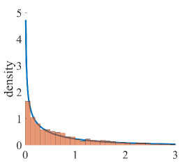
(a) $N=30$

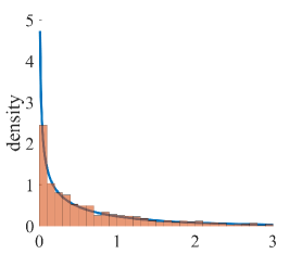
(b) $N=100$

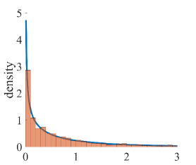
(c) $N=500$

Figure 2: Empirical distribution $N\times\mathcal{D}(\hat{\mathbb{P}}^{N})$ over 2,000 replications (histogram) versus the limiting Chi-square distribution (blue curve) with different sample sizes $N$.

In the second experiments, we show that our proposed Wasserstein projection hypothesis test has the desired coverage property. We generate $N\in\{30,100,500,1000,2000\}$ i.i.d. samples from $\mathbb{P}$ and compute the estimate $\hat{S}$ defined in Section 5.2 and the empirical covariance using the sample data. For the kernel estimator $\hat{S}$, we use the standard Gaussian kernel and choose the bandwidth $h=N^{-1/5}$, where the results listed below are not sensitive to the constant. We repeat the procedure for 2,000 replications and report the rejection probability at different significant values of $\alpha\in\{0.1,0.05,0.01\}$ in Table 4. We can observe that when $N>100$, the rejection probability is closed to the desired level $\alpha$.

Table 4: Comparison of the null rejection probabilities of probabilistic equal opportunity tests with different significance levels $\alpha$ and test sample sizes $N$.

$\alpha$	0.10	0.05	0.01
$N=30$	0.2875	0.2255	0.1415
$N=100$	0.0945	0.0540	0.0250
$N=500$	0.0895	0.0450	0.0085
$N=1000$	0.0900	0.0430	0.0065
$N=2000$	0.0870	0.0460	0.0080

Appendix B.2 The Description of Datasets

Followings show brief descriptions of datasets: Arrhythmia, COMPAS and Drug (Fehrman et al., 2017) provided in Section 6.

• Arrhythmia is from UCI repository, where the aim of this data set is to distinguish between the presence and absence of cardiac arrhythmia and classify it in one of the 16 groups. The dataset consists of 452 samples and we use the first 12 features among which the gender is the sensitive feature. For our purpose, we construct binary labels between ‘class 01’ (‘normal’) and all other classes (different classes of arrhythmia and unclassified ones).

• COMPAS (Correctional Offender Management Profiling for Alternative Sanctions) is a commerical tool used by judges, probation and parole officers to estimate a criminal defendant’s likelihood to re-offend algorithmically. The COMPAS dataset contains the criminal records within 2 years after the decision. We use race (African-American and Caucasian, which accounts for 5278 samples) as the sensitive attribute.

• Drug (Fehrman et al., 2017) contains answers of 1885 participants on their use of 17 legal and illegal drugs. We concern the cannabis usage as a binary problem, where the label is ‘Never used’ VS ‘Others’ (‘used’). There are 12 features including age, gender, education, country, ethnicity, NEO-FFI-R measurements, impulsiveness measured by BIS-11 and sensation seeing measured by ImpSS. Among those, we choose ethnicity (black vs others) as the sensitive attribute.

References

• Barocas & Selbst (2016) Barocas, S. and Selbst, A. D. Big data’s disparate impact. California Law Review, 104:671–732, 2016.
• Berk et al. (2018) Berk, R., Heidari, H., Jabbari, S., Kearns, M., and Roth, A. Fairness in criminal justice risk assessments: The state of the art. Sociological Methods & Research, pp.  0049124118782533, 2018.
• Besse et al. (2018) Besse, P., del Barrio, E., Gordaliza, P., and Loubes, J.-M. Confidence intervals for testing disparate impact in fair learning. arXiv preprint arXiv:1807.06362, 2018.
• Billingsley (2013) Billingsley, P. Convergence of Probability Measures. John Wiley & Sons, 2013.
• Black et al. (2020) Black, E., Yeom, S., and Fredrikson, M. Fliptest: fairness testing via optimal transport. In Proceedings of the 2020 Conference on Fairness, Accountability, and Transparency, pp.  111–121, 2020.
• Blanchet et al. (2019) Blanchet, J., Kang, Y., and Murthy, K. Robust Wasserstein profile inference and applications to machine learning. Journal of Applied Probability, 56(3):830–857, 2019.
• Buolamwini & Gebru (2018) Buolamwini, J. and Gebru, T. Gender shades: Intersectional accuracy disparities in commercial gender classification. In Conference on Fairness, Accountability and Transparency, pp.  77–91, 2018.
• Calders & Verwer (2010) Calders, T. and Verwer, S. Three naive Bayes approaches for discrimination-free classification. Data Mining and Knowledge Discovery, 21(2):277–292, 2010.
• Chouldechova (2017) Chouldechova, A. Fair prediction with disparate impact: A study of bias in recidivism prediction instruments. Big Data, 5(2):153–163, 2017.
• Chouldechova & Roth (2020) Chouldechova, A. and Roth, A. A snapshot of the frontiers of fairness in machine learning. Communications of the ACM, 63(5):82–89, 2020.
• Cisneros-Velarde et al. (2020) Cisneros-Velarde, P., Petersen, A., and Oh, S.-Y. Distributionally robust formulation and model selection for the graphical lasso. In International Conference on Artificial Intelligence and Statistics, pp.  756–765. PMLR, 2020.
• Corbett-Davies et al. (2017) Corbett-Davies, S., Pierson, E., Feller, A., Goel, S., and Huq, A. Algorithmic decision making and the cost of fairness. In Proceedings of the 23rd ACM SIGKDD International Conference on Knowledge Discovery and Data Mining, pp.  797–806, 2017.
• Dastin (2018) Dastin, J. Amazon scraps secret AI recruiting tool that showed bias against women. San Fransico, CA: Reuters. Retrieved on October, 9:2018, 2018.
• Datta et al. (2015) Datta, A., Tschantz, M. C., and Datta, A. Automated experiments on ad privacy settings: A tale of opacity, choice, and discrimination. Proceedings on Privacy Enhancing Technologies, 2015(1):92–112, 2015.
• DiCiccio et al. (2020) DiCiccio, C., Vasudevan, S., Basu, K., Kenthapadi, K., and Agarwal, D. Evaluating fairness using permutation tests. In Proceedings of the 26th ACM SIGKDD International Conference on Knowledge Discovery & Data Mining, pp.  1467–1477, 2020.
• Donini et al. (2018) Donini, M., Oneto, L., Ben-David, S., Shawe-Taylor, J. S., and Pontil, M. Empirical risk minimization under fairness constraints. In Advances in Neural Information Processing Systems, pp. 2791–2801, 2018.
• Dua & Graff (2017) Dua, D. and Graff, C. UCI machine learning repository, 2017. URL http://archive.ics.uci.edu/ml.
• Durrett (2019) Durrett, R. Probability: Theory and Examples. Cambridge University Press, 2019.
• Dwork et al. (2012) Dwork, C., Hardt, M., Pitassi, T., Reingold, O., and Zemel, R. Fairness through awareness. In Proceedings of the 3rd Innovations in Theoretical Computer Science Conference, pp.  214–226, 2012.
• Fehrman et al. (2017) Fehrman, E., Muhammad, A. K., Mirkes, E. M., Egan, V., and Gorban, A. N. The five factor model of personality and evaluation of drug consumption risk. In Data Science, pp.  231–242. Springer, 2017.
• Garg et al. (2019) Garg, S., Perot, V., Limtiaco, N., Taly, A., Chi, E. H., and Beutel, A. Counterfactual fairness in text classification through robustness. In Proceedings of the 2019 AAAI/ACM Conference on AI, Ethics, and Society, pp.  219–226, 2019.
• Gordaliza et al. (2019) Gordaliza, P., Barrio, E. D., Fabrice, G., and Loubes, J.-M. Obtaining fairness using optimal transport theory. In Proceedings of the 36th International Conference on Machine Learning, pp.  2357–2365, 2019.
• Grgic-Hlaca et al. (2016) Grgic-Hlaca, N., Zafar, M. B., Gummadi, K. P., and Weller, A. The case for process fairness in learning: Feature selection for fair decision making. In NIPS Symposium on Machine Learning and the Law, volume 1, pp.  2, 2016.
• Härdle (1990) Härdle, W. Applied Nonparametric Regression. Cambridge University Press, 1990.
• Hardt et al. (2016) Hardt, M., Price, E., Price, E., and Srebro, N. Equality of opportunity in supervised learning. In Advances in Neural Information Processing Systems 29, pp. 3315–3323, 2016.
• Hui et al. (2021) Hui, Y., Xie, J., Blanchet, J., and Glynn, P. Empirical optimal transport projections with non-symmetric costs. preprint, 2021.
• John et al. (2020) John, P. G., Vijaykeerthy, D., and Saha, D. Verifying individual fairness in machine learning models. In Conference on Uncertainty in Artificial Intelligence, pp. 749–758. PMLR, 2020.
• Kleinberg et al. (2018) Kleinberg, J., Ludwig, J., Mullainathan, S., and Rambachan, A. Algorithmic fairness. In AEA Papers and Proceedings, volume 108, pp.  22–27, 2018.
• Lipton et al. (2018) Lipton, Z., McAuley, J., and Chouldechova, A. Does mitigating ML’s impact disparity require treatment disparity? In Advances in Neural Information Processing Systems, pp. 8125–8135, 2018.
• Makhlouf et al. (2020) Makhlouf, K., Zhioua, S., and Palamidessi, C. On the applicability of ML fairness notions. arXiv preprint arXiv:2006.16745, 2020.
• Manrai et al. (2016) Manrai, A. K., Funke, B. H., Rehm, H. L., Olesen, M. S., Maron, B. A., Szolovits, P., Margulies, D. M., Loscalzo, J., and Kohane, I. S. Genetic misdiagnoses and the potential for health disparities. New England Journal of Medicine, 375(7):655–665, 2016.
• Mehrabi et al. (2019) Mehrabi, N., Morstatter, F., Saxena, N., Lerman, K., and Galstyan, A. A survey on bias and fairness in machine learning. arXiv preprint arXiv:1908.09635, 2019.
• MultiMedia LLC (2016) MultiMedia LLC. Machine Bias, 2016. Available at https://www.propublica.org/article/machine-bias-risk-assessments-in-criminal-sentencing.
• Owen (2001) Owen, A. B. Empirical Likelihood. CRC Press, 2001.
• Pleiss et al. (2017) Pleiss, G., Raghavan, M., Wu, F., Kleinberg, J., and Weinberger, K. Q. On fairness and calibration. In Advances in Neural Information Processing Systems, pp. 5680–5689, 2017.
• Saleiro et al. (2018) Saleiro, P., Kuester, B., Hinkson, L., London, J., Stevens, A., Anisfeld, A., Rodolfa, K. T., and Ghani, R. Aequitas: A bias and fairness audit toolkit. arXiv preprint arXiv:1811.05577, 2018.
• Silvia et al. (2020) Silvia, C., Ray, J., Tom, S., Aldo, P., Heinrich, J., and John, A. A general approach to fairness with optimal transport. In Proceedings of the AAAI Conference on Artificial Intelligence, volume 34, pp.  3633–3640, 2020.
• Taskesen et al. (2021) Taskesen, B., Blanchet, J., Kuhn, D., and Nguyen, V. A. A statistical test of probabilistic fairness. Accepted to ACM Conference on Fairness, Accountability, and Transparency, 2021.
• Tramer et al. (2017) Tramer, F., Atlidakis, V., Geambasu, R., Hsu, D., Hubaux, J.-P., Humbert, M., Juels, A., and Lin, H. Fairtest: Discovering unwarranted associations in data-driven applications. In 2017 IEEE European Symposium on Security and Privacy (EuroS&P), pp.  401–416. IEEE, 2017.
• Tsybakov (2008) Tsybakov, A. B. Introduction to Nonparametric Estimation. Springer, 2008.
• Villani (2008) Villani, C. Optimal Transport: Old and New, volume 338. Springer, 2008.
• Xue et al. (2020) Xue, S., Yurochkin, M., and Sun, Y. Auditing ML models for individual bias and unfairness. In International Conference on Artificial Intelligence and Statistics, pp.  4552–4562. PMLR, 2020.
• Zafar et al. (2017) Zafar, M. B., Valera, I., Gomez Rodriguez, M., and Gummadi, K. P. Fairness beyond disparate treatment & disparate impact: Learning classification without disparate mistreatment. In Proceedings of the 26th International Conference on World Wide Web, pp.  1171–1180, 2017.
• Zehlike et al. (2020) Zehlike, M., Hacker, P., and Wiedemann, E. Matching code and law: achieving algorithmic fairness with optimal transport. Data Mining and Knowledge Discovery, 34(1):163–200, 2020.