Hilbert’s spacefilling curve described by automatic, regular, and synchronized sequences

Abstract

We describe Hilbert’s spacefilling curve in several different ways: as an automatic sequence of directions, as a regular and synchronized sequence of coordinates of lattice points encountered, and as an automatic bitmap image.

1 Introduction

In 1891 David Hilbert famously described the construction of a continuous curve that fills the unit square [13]. So many papers on this topic have been published since then (for example, see [9, 10, 16, 8]) that it seems difficult to say anything new about it. Nevertheless, we’ll try. We will describe the curve in three different ways: as a $4$-automatic sequence, as a $4$-regular sequence, and as a $(4,2,2)$-synchronized sequence. An interesting feature of our approach is that in each case, we “guess” the correct representation, and then use the theorem-prover Walnut to prove our guess is correct [15].

Instead of filling the unit square, we will treat a version that visits every non-negative pair of integers, starting from the origin $(0,0)$. At each stage we take the figure constructed so far, make four copies, flip each copy appropriately (Figure 1), and join them together, as illustrated in Figure 2.

Let us agree to write $\tt U$ for up, $\tt D$ for down, $\tt R$ for right, and $\tt L$ for left. Thus $A_{n}$, the $n$’th generation of the curve, can be written as a string over the alphabet $\{{\tt U,D,R,L}\}$, and it is easy to see that in fact $|A_{n}|=4^{n}-1$. Note that the moves inserted to connect the pieces depend on the parity: to go from $A_{n}$ to $A_{n+1}$ when $n$ is odd, we successively insert $\tt RUL$ to connect the pieces, but when $n$ is even, we successively insert $\tt URD$.

The first four generations of the curve are encoded as follows:

$$A_{0} =\epsilon$$

$$A_{1} ={\tt URD}$$

$$A_{2} ={\tt URDRRULURULLDLU}$$

$$A_{3} ={\tt URDRRULURULLDLUURULUURDRURDDLDRRRULUURDRURDDLDRDDLULLDRDLDRRURD}$$

Notice that $A_{n}$ is a prefix of $A_{n+1}$ for all $n\geq 0$. So we can let

$${\bf HC}=(h_{n})_{n\geq 0}={\tt URDRRULURULLD}\cdots$$

be the unique infinite string of which $A_{1},A_{2},A_{3},\ldots$ are all prefixes.

Furthermore $A_{n}$ is a path from $(0,0)$ to $(2^{n}-1,0)$ if $n$ is odd, and a path from $(0,0)$ to $(0,2^{n}-1)$ if $n$ is even.

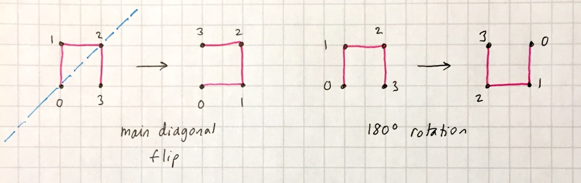
Figure 1: How one generation follows from the previous.

2 By recurrence

We now wish to write a recurrence for the $A_{n}$. We define the codings $t_{D},t_{H}$ as follows: $t_{D}$ is a flip about the main diagonal, and hence $t_{D}({\tt UDRL})=\tt RLUD$, while $t_{H}$ is a $180^{\circ}$ rotation, that is, $t_{H}({\tt UDRL})=\tt DULR$.

This gives us a formula to compute $A_{n}$, namely

$$A_{0} =\epsilon$$

$$A_{2n+1} =A_{2n}\,{\tt U}\,t_{D}(A_{2n})\,{\tt R}\,t_{D}(A_{2n})\,{\tt D}\,t_{H}(A_{2n})$$ (1)

$$A_{2n+2} =A_{2n+1}\,{\tt R}\,t_{D}(A_{2n+1})\,{\tt U}\,t_{D}(A_{2n+1})\,{\tt L}\,t_{H}(A_{2n+1})$$

for $n\geq 0$.

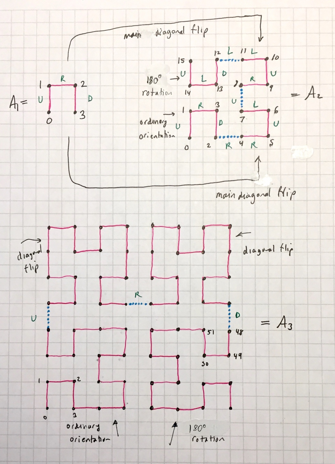
Figure 2: The first three generations of the Hilbert curve.

3 As image of fixed point of morphism or automatic sequence

We use the notation $\Sigma_{k}=\{0,1,\ldots,k-1\}$, and $(n)_{k}$ denotes the canonical base-$k$ representation of $n$, starting with the most significant digit.

Recall that a sequence $(a_{n})_{n\geq 0}$ is $k$-automatic if its $k$-kernel

$$\{(a_{k^{e}n+i})_{n\geq 0}\,:\,e\geq 0,0\leq i<k^{e}\}$$

is of finite cardinality [3, §6.6]. Alternatively, $(a_{n})_{n\geq 0}$ is $k$-automatic if there is a deterministic finite automaton with output (DFAO) that reads $(n)_{k}$ as input and reaches a state with output $a_{n}$.

The fact that the length of the $i$’th generation $A_{i}$ is so close to $4^{i}$ strongly suggests that $H$ might be $4$-automatic.

To try to determine the DFAO, we can use a “guessing procedure” based on the Myhill-Nerode theorem [17, §3.9] to find a good candidate, and then use a theorem-prover to prove that our guess is correct. We repeat this strategy throughout the paper.

We find an $8$-state DFAO $(Q,\Sigma,\Gamma,\delta,q_{0},\tau)$ as follows:

• $Q=\{0,1,\ldots,7\}$;

• $\Sigma=\Sigma_{4}$;

• $\Gamma=\{{\tt U,R,D,L}\}$;

• $q_{0}=0$;

• $\delta(q,i)$ and $\tau$ are defined as in Table 1.

  	0	1	2	3	$\tau(q)$
  0	0	1	2	3	U
  1	1	0	4	5	R
  2	1	0	4	6	D
  3	7	6	5	0	R
  4	0	1	2	7	L
  5	6	7	3	1	U
  6	6	7	3	2	L
  7	7	6	5	4	D

  Table 1: DFAO for the sequence $\bf HC$.

In Walnut this DFAO can be represented by the name HC. Because Walnut currently does not allow letters as output, we use the recoding of the output given by the correspondence ${\tt U}\leftrightarrow{\tt 0}$, ${\tt R}\leftrightarrow{\tt 1}$, ${\tt D}\leftrightarrow{\tt 2}$, ${\tt L}\leftrightarrow{\tt 3}$.

We can verify that this automaton is correct by using Walnut. From Eq. (1), it suffices to check that for all $n\geq 0$ we have

$${\bf HC}[0] ={\tt U}$$ (2)

$${\bf HC}[4^{n}..2\cdot 4^{n}-1] =t_{D}({\bf HC}[0..4^{n}-1])$$ (3)

$${\bf HC}[2\cdot 4^{n}..3\cdot 4^{n}-2] =t_{D}({\bf HC}[0..4^{n}-2])$$ (4)

$${\bf HC}[3\cdot 4^{n}-1] =\begin{cases}{\tt L},&\text{if $n$ odd;}\\ {\tt D},&\text{if $n$ even;}\end{cases}$$ (5)

$${\bf HC}[3\cdot 4^{n}..4^{n+1}-2] =t_{H}({\bf HC}[0..4^{n}-2])$$ (6)

$${\bf HC}[4^{n}-1] =\begin{cases}{\tt R},&\text{if $n$ odd;}\\ {\tt U},&\text{if $n$ even.}\end{cases}$$ (7)

which we can do with Walnut as follows:

reg power4 msd_4 "0*10*":
reg evenpower4 msd_4 "0*1(00)*":
reg oddpower4 msd_4 "0*10(00)*":
eval test2 "?msd_4 HC[0]=@0":
eval test3 "?msd_4 Ax,t ($power4(x) & t<x) =>
     ((HC[t]=@0 <=> HC[x+t]=@1) & (HC[t]=@1 <=> HC[x+t]=@0)
     &(HC[t]=@2 <=> HC[x+t]=@3) & (HC[t]=@3 <=> HC[x+t]=@2))":
eval test4 "?msd_4 Ax,t ($power4(x) & t+1<x) =>
     ((HC[t]=@0 <=> HC[2*x+t]=@1) & (HC[t]=@1 <=> HC[2*x+t]=@0)
     &(HC[t]=@2 <=> HC[2*x+t]=@3) & (HC[t]=@3 <=> HC[2*x+t]=@2))":
eval test5 "?msd_4 Ax ($oddpower4(x) => HC[3*x-1]=@3) &
     ($evenpower4(x) => HC[3*x-1]=@2)":
eval test6 "?msd_4 Ax,t ($power4(x) & t+1<x) =>
     ((HC[t]=@0 <=> HC[3*x+t]=@2) & (HC[t]=@1 <=> HC[3*x+t]=@3)
     &(HC[t]=@2 <=> HC[3*x+t]=@0) & (HC[t]=@3 <=> HC[3*x+t]=@1))":
eval test7 "?msd_4 Ax ($oddpower4(x) => HC[x-1]=@1) &
     ($evenpower4(x) => HC[x-1]=@0)":

and everything returns true.

4 As system of coordinates and a $4$-regular sequence

Recall that a $k$-regular sequence is a generalization of automatic sequence. Being $k$-regular means there is a finite subset $S$ of the $k$-kernel such that each element of the $k$-kernel can be written as a linear combination of elements of $S$ [1, 2].

Suppose we start at $(x_{0},y_{0}):=(0,0)$ and perform unit steps according to the letters specified by $\bf HC$. Thus we have

$$(x_{n+1},y_{n+1})=(x_{n},y_{n})+\begin{cases}(1,0),&\text{ if ${\bf HC}[n]={\tt R}$};\\ (-1,0),&\text{ if ${\bf HC}[n]={\tt L}$};\\ (0,1),&\text{ if ${\bf HC}[n]={\tt U}$};\\ (0,-1),&\text{ if ${\bf HC}[n]={\tt D}$};\end{cases}$$

This gives us a sequence of ordered pairs specifying the $x$-$y$ coordinates of the $n$’th point along the curve. Table 2 gives the few values of $((x_{n},y_{n}))_{n\geq 0}$. The sequence $(x_{n})_{n\geq 0}$ is sequence A059252 and $(y_{n})_{n\geq 0}$ is A059253 in [19].

$n$	0	1	2	3	4	5	6	7	8	9	10	11	12	13	14	15
$x_{n}$	0	0	1	1	2	3	3	2	2	3	3	2	1	1	0	0
$y_{n}$	0	1	1	0	0	0	1	1	2	2	3	3	3	2	2	3

Table 2: First few values of $(x_{n},y_{n})$ for the Hilbert curve.

In this section we show that $(x_{n},y_{n})_{n\geq 0}$, the sequence of coordinates traversed by the Hilbert curve, is $4$-regular. Actually, this follows immediately from [1, Theorem 3.1], but applying this theorem is somewhat messy.

Recall that a linear representation for a $k$-regular sequence $(a_{n})_{n\geq 0}$ consists of a row vector $v$, a matrix-valued morphism $\gamma$, and a column vector $w$ such that $a_{n}=v\gamma((n)_{k})w$ for all $n\geq 0$. The dimension of $w$ is called the rank of the linear representation; see [6].

A “guessing procedure” for $k$-regular sequences suggests that the $4$-kernel of $(x_{n})_{n\geq 0}$ is contained in the linear span of the $5$ subsequences

$$\{(x_{n})_{n\geq 0},\ (x_{4n})_{n\geq 0},\ (x_{4n+1})_{n\geq 0},\ (x_{4n+2})_{n\geq 0},\ (x_{16n})_{n\geq 0}\},$$

and the same for $(y_{n})_{n\geq 0}$. We can then “guess” a number of candidate relations for elements of the $4$-kernel for both $x_{n}$ and $y_{n}$. Assuming the guessed relations are correct, by standard techniques, we can deduce a rank-$5$ base-$4$ linear representation for $((x_{n},y_{n}))_{n\geq 0}$, namely:

$$(x_{n},y_{n})=v\gamma((n)_{4})w,$$

where $(n)_{4}$ is the base-$4$ representation of $n$ and

$$v=\left[\begin{array}[]{ccccc}0&0&0&1&0\\ 0&0&1&1&0\end{array}\right];\quad\gamma(0)=\left[\begin{array}[]{ccccc}0&0&0&0&-4\\ 1&0&-1&-1&4\\ 0&0&1&0&0\\ 0&0&0&1&0\\ 0&1&1&1&1\\ \end{array}\right];\quad\gamma(1)=\left[\begin{array}[]{ccccc}0&0&0&0&-4\\ 0&0&0&-1&0\\ 1&-2&-3&-2&4\\ 0&2&3&3&0\\ 0&1&1&1&1\end{array}\right];$$

$$\gamma(2)=\left[\begin{array}[]{ccccc}0&0&0&0&-4\\ 0&-2&-2&-3&0\\ 0&0&-1&0&0\\ 1&2&3&3&4\\ 0&1&1&1&1\end{array}\right];\quad\gamma(3)=\left[\begin{array}[]{ccccc}0&0&0&0&-4\\ 1&-3&-2&-2&1\\ -1&2&1&2&-4\\ 1&1&1&0&7\\ 0&1&1&1&1\end{array}\right];\quad w=\left[\begin{array}[]{ccccc}1\\ 0\\ 0\\ 0\\ 0\\ \end{array}\right].$$

We now prove that this is indeed a linear representation for $((x_{n},y_{n}))_{n\geq 0}$, in a somewhat roundabout way.

Recall that a finite-state transducer $T$ maps input strings to output strings. The output associated with an input are the string or strings arising from the concatenation of the outputs of all transitions, provided processing the string ends in a final state of $T$. We allow a transducer to be nondeterministic. A transducer is functional if every input results in at most one output [17, §3.5]. We need a lemma.

Lemma 1.

Let $(f(n))_{n\geq 0}$ be a $k$-regular sequence, and let $\Sigma_{k}=\{0,1,\ldots,k-1\}$. Let $T=(Q,\Sigma_{k},\Sigma_{k},\delta,q_{0},F,\rho)$ be a nondeterministic functional finite-state transducer with transitions on single letters only, but allowing arbitrary words as outputs on each transition. More precisely,

• $Q=\{q_{0},\ldots,q_{r-1}\}$;

• $\delta:Q\times\Sigma_{k}\rightarrow Q$ is the transition function; and

• $\rho:Q\times\Sigma_{k}\rightarrow\Sigma_{k}^{*}$ is the output function;

• $F$ is a set of final states.

Let the domain of $\delta$ and $\rho$ be extended to $\Sigma_{k}^{*}$ in the obvious way. Define $g(n)=f(T((n)_{k})))$. Then $(g(n))_{n\geq 0}$ is also a $k$-regular sequence.

Proof.

Let $(v,\mu,w)$ be a rank-$s$ linear representation for $f$. We create a linear representation $(v^{\prime},\mu^{\prime},w^{\prime})$ for $g$.

The idea is that $\mu^{\prime}(a)$, $0\leq a<k$, is an $n\times n$ matrix, where $n=rs$. It is easiest to think of $\mu^{\prime}(a)$ as an $r\times r$ matrix, where each entry is itself an $s\times s$ matrix. In this interpretation, $(\mu^{\prime}(a))_{i,j}=\mu(\rho(q_{i},a))$ if $\delta(q_{i},a)=q_{j}$.

An easy induction now shows that if $\delta(q_{i},x)=q_{j}$ and $\rho(q_{i},x)=y$, then $(\mu^{\prime}(x))_{i,j}=\mu(y)$. If we now let $v^{\prime}$ be the vector $[v\quad 0\quad\cdots\quad 0]$ and $w^{\prime}$ be the column vector with $w$’s in the positions of the final states and $0$’s otherwise, then it follows that $v^{\prime}\mu^{\prime}(x)w^{\prime}=v\mu(T(x))w$. This gives a linear representation for $(g(n))_{n\geq 0}$. ∎

In particular, there is a simple finite-state transducer that, when applied to the base-$k$ representation of $n$ gives the representation of $n+1$. For $k=4$ this transducer is depicted in Figure 3 below:

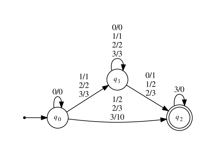
Figure 3: A transducer mapping $(n)_{4}$ to $(n+1)_{4}$

So from the guessed linear representation for $(x_{n})_{n\geq 0}$ we easily deduce a linear representation for $(x_{n+1})_{n\geq 0}$. It is of rank $15$.

Now from these two linear representations, we can use an obvious “tensor product”-style construction to get the linear representation for the first difference sequence $(x_{n+1}-x_{n})_{n\geq 0}$. This produces a linear representation of rank $20$. We can do the same thing with $(y_{n})_{n\geq 0}$.

Now we can use the Berstel-Reutenauer minimization algorithm [6, §3.3] for linear representations to get an equivalent minimized linear representation $(v^{\prime},\gamma^{\prime},w^{\prime})$ for $((x_{n+1}-x_{n},y_{n+1}-y_{n}))_{n\geq 0}$. Here is what it looks like:

$$v^{\prime}=\left[\begin{array}[]{ccc}1&0&0\\ 0&1&0\end{array}\right];\quad\gamma^{\prime}(0)=\left[\begin{array}[]{ccc}1&0&0\\ 0&1&0\\ 0&1&0\end{array}\right];\quad\gamma^{\prime}(1)=\left[\begin{array}[]{ccccc}0&1&0\\ 1&0&0\\ 1&0&0\end{array}\right];$$

$$\gamma^{\prime}(2)=\left[\begin{array}[]{ccc}0&0&1\\ 1&-1&1\\ 1&-1&1\end{array}\right];\quad\gamma^{\prime}(3)=\left[\begin{array}[]{ccc}-1&1&-1\\ 0&0&-1\\ 0&-1&0\end{array}\right];\quad w^{\prime}=\left[\begin{array}[]{ccc}0\\ 1\\ 0\\ \end{array}\right].$$

Now we use the “semigroup trick” (see [12, pp. 951,954]) to find an automaton for the first difference sequence $((x_{n+1}-x_{n},y_{n+1}-y_{n}))_{n\geq 0}$ and prove that the resulting automaton has only finitely many states. And no surprise—it is the same automaton we started with, the one in Section 3. This shows that our guessed linear representation for $((x_{n},y_{n}))_{n\geq 0}$ was indeed correct.

The advantage to the representation as a $4$-regular sequence is that we can compute $(x_{n},y_{n})$ in time linear in the number of bits of $n$: we express $n$ in base 4, and then multiply the appropriate vectors and $O(\log_{4}n)$ matrices.

5 As a synchronized function

Finally, perhaps the most interesting representation of the Hilbert curve is that $n$ and $(x_{n},y_{n})$ are synchronized, but only if we represent $n$, $x_{n}$, and $y_{n}$ in the right way. The right way is to represent $n$ in base $4$, but represent $x_{n}$ and $y_{n}$ in base $2$! In other words, the triple $(n,x_{n},y_{n})$ is $(4,2,2)$-synchronized [11].

Here our guessing procedure guesses a 10-state automaton ${\tt HS}=(Q,\Sigma,\delta,q_{0},F)$, given below. Here

• $Q=\{0,1,\ldots,9\}$;

• $\Sigma=\Sigma_{4}\times\Sigma_{2}\times\Sigma_{2}$;

• $q_{0}=0$;

• $F=\{0,2,3,5,6,7\}$;

and $\delta$ is represented in Table 3. (All transitions not listed go to a dead state that is not accepting, which just loops to itself on each input.)

• verify that indeed $\tt HS$ represents a synchronized function:

  • for each $n$ there is a pair $(x,y)$ such that ${\tt HS}[n][x][y]$ is true

  • for each $n$ there is only one pair $(x,y)$ such that ${\tt HS}[n][x][y]$ is true

• verify that ${\tt HS}[0][0][0]=0$;

• verify that if ${\tt HS}[n][x][y]$ and ${\tt HS}[n+1][x^{\prime}][y^{\prime}]$ both hold, then $(x^{\prime}-x,y^{\prime}-x)$ corresponds to the appropriate move ${\tt U,D,R,L}$ computed by the automaton in Section 3.

eval fn1 "An Ex,y HS[?msd_4 n][x][y]=@1":
# f(n) takes an ordered pair value for each n

eval fn2 "An,x,y,xp,yp (HS[?msd_4 n][x][y]=@1 & HS[?msd_4 n][xp][yp]=@1) => (x=xp & y=yp)":
# f(n) takes only one value for each n

eval check_up "An (HC[?msd_4 n]=@0 <=> Ex,xp,y,yp HS[?msd_4 n][x][y]=@1 &
    HS[?msd_4 n+1][xp][yp]=@1 & xp=x & yp=y+1)":

eval check_right "An (HC[?msd_4 n]=@1 <=> Ex,xp,y,yp HS[?msd_4 n][x][y]=@1 &
    HS[?msd_4 n+1][xp][yp]=@1 & xp=x+1 & yp=y)":

eval check_down "An (HC[?msd_4 n]=@2 <=> Ex,xp,y,yp HS[?msd_4 n][x][y]=@1 &
    HS[?msd_4 n+1][xp][yp]=@1 & xp=x & yp+1=y)":

eval check_left "An (HC[?msd_4 n]=@3 <=> Ex,xp,y,yp HS[?msd_4 n][x][y]=@1 &
    HS[?msd_4 n+1][xp][yp]=@1 & xp+1=x & yp=y)":

and Walnut returns true.

Finally, we can use Walnut to verify that every pair of natural numbers $(x,y)$ is hit by one and exactly one $n$, so our curve is indeed space-filling:

eval allhit "Ax,y En HS[?msd_4 n][x][y]=@1":
eval hitonce "An,np,x,y (HS[?msd_4 n][x][y]=@1 & HS[?msd_4 np][x][y]=@1)
     => (?msd_4 n=?msd_4 np)":

and Walnut returns true for both.

$q$	$t=[i,j,k]$	$\delta(q,t)$	$q$	$t=[i,j,k]$	$\delta(q,t)$
0	$[0,0,0]$	0	5	$[0,0,0]$	5
0	$[1,0,1]$	3	5	$[1,0,1]$	9
0	$[1,1,0]$	1	5	$[1,1,0]$	6
0	$[2,1,1]$	5	5	$[2,1,1]$	0
0	$[3,0,1]$	4	5	$[3,0,1]$	7
0	$[3,1,0]$	2	5	$[3,1,0]$	8
1	$[0,0,0]$	3	6	$[0,0,0]$	9
1	$[1,1,0]$	6	6	$[1,1,0]$	1
1	$[2,1,1]$	6	6	$[2,1,1]$	1
1	$[3,0,1]$	7	6	$[3,0,1]$	4
2	$[0,1,1]$	4	7	$[0,1,1]$	8
2	$[1,0,1]$	8	7	$[1,1,0]$	4
2	$[2,0,0]$	8	7	$[2,0,0]$	4
2	$[3,1,0]$	9	7	$[3,0,1]$	1
3	$[0,0,0]$	1	8	$[0,1,1]$	7
3	$[1,0,1]$	9	8	$[1,0,1]$	2
3	$[2,1,1]$	9	8	$[2,0,0]$	2
3	$[3,1,0]$	8	8	$[3,1,0]$	3
4	$[0,1,1]$	2	9	$[0,0,0]$	6
4	$[1,1,0]$	7	9	$[1,0,1]$	3
4	$[2,0,0]$	7	9	$[2,1,1]$	3
4	$[3,0,1]$	6	9	$[3,1,0]$	2

Table 3: The synchronized automaton for coordinates of Hilbert’s curve.

From the synchronized automaton, given $(n)_{4}=a_{1}a_{2}\cdots a_{t}$, the base-$4$ representation of $n$, we can easily determine $(x_{n},y_{n})$, by intersecting the automaton with an automaton accepting those strings of the form $[a_{1},*,*][a_{2},*,*]\cdots[a_{t},*,*]$, where $*$ denotes either $0$ or $1$. In the resulting automaton, only one path is accepting, and it can easily be found in $O(t)$ time through breadth-first or depth-first search.

But the reverse is also true: given the base-$2$ representations of $(x,y)$, we can easily determine the $n$ for which $(x_{n},y_{n})=(x,y)$, using the same idea.

6 As an automatic bitmap image

With the aid of the synchronized representation for HS, we can easily produce a bitmap image of each generation of the Hilbert curve, as previously done in [18, Fig. 6].

To do so, we “expand” the curve, inserting rows and column that are blank, except for when they connect two consecutive points of the curve. The following Walnut code produces a DFA $hp describing a bitmap image of the Hilbert curve.

def even "Em n=2*m":
def odd "Em n=2*m+1":
def hp "($even(x) & $even(y)) |
($even(x) & $odd(y) &
(En (HS[?msd_4 n][x/2][(y-1)/2]=@1 & HS[?msd_4 n+1][x/2][(y+1)/2]=@1)
|(HS[?msd_4 n][x/2][(y+1)/2]=@1 & HS[?msd_4 n+1][x/2][(y-1)/2]=@1)) |
($odd(x) & $even(y) &
(En (HS[?msd_4 n][(x-1)/2][y/2]=@1 & HS[?msd_4 n+1][(x+1)/2][y/2]=@1)
|(HS[?msd_4 n][(x+1)/2][y/2]=@1 & HS[?msd_4 n+1][(x-1)/2][y/2]=@1))":

For example, for generation $7$ we get the image in Figure 4.

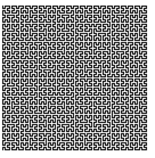
Figure 4: Generation $7$ of the Hilbert curve.

References

- [1] J.-P. Allouche and J. O. Shallit. The ring of -regular sequences. Theoret. Comput. Sci. 98 (1992), 163–197.
- [2] J.-P. Allouche and J. O. Shallit. The ring of -regular sequences, II. Theoret. Comput. Sci. 307 (2003), 3–29.
- [3] J.-P. Allouche and J. Shallit. Automatic Sequences: Theory, Applications, Generalizations. Cambridge University Press, 2003.
- [4] J. Arndt. Matters Computational—Ideas, Algorithms, Source Code. Springer, 2011.
- [5] M. Beeler, R. W. Gosper, and R. Schroeppel. Hakmem. MIT Artificial Intelligence Laboratory, Report AIM 239, February 1972. Available at https://w3.pppl.gov/~hammett/work/2009/AIM-239-ocr.pdf.
- [6] J. Berstel and C. Reutenauer. Noncommutative Rational Series with Applications, Vol. 137 of Encyclopedia of Mathematics and Its Applications. Cambridge University Press, 2010.
- [7] T. Bially. Space-filling curves: their generation and their application to bandwidth reduction. IEEE Trans. Info. Theory IT-15 (1969), 658–664.
- [8] G. Breinholt and C. Schierz. Algorithm 781: Generating Hilbert’s space-filling curve by recursion. ACM Trans. Math. Software 24 (1998), 184–189.
- [9] A. R. Butz. Convergence with Hilbert’s space filling curve. J. Comput. System Sci. 3 (1969), 128–146.
- [10] A. R. Butz. Alternative algorithm for Hilbert’s space-filling curve. IEEE Trans. Comput. 20 (1971), 424–426.
- [11] A. Carpi and C. Maggi. On synchronized sequences and their separators. RAIRO Inform. Théor. App. 35 (2001), 513–524.
- [12] C. F. Du, H. Mousavi, L. Schaeffer, and J. Shallit. Decision algorithms for Fibonacci-automatic words III: enumeration and abelian properties. Int. J. Found. Comput. Sci. 27 (2016) 943–963.
- [13] D. Hilbert. Über die stetige Abbildung einer Linie auf ein Flächenstück. Math. Annalen 38 (1891), 459–460.
- [14] H. V. Jagadish. Analysis of the Hilbert curve for representing two-dimensional space. Info. Process. Letters 62 (1997), 17–22.
- [15] H. Mousavi. Automatic theorem proving in Walnut, 2016. Preprint available at http://arxiv.org/abs/1603.06017.
- [16] H. Sagan. Space-Filling Curves. Springer, 1994.
- [17] J. Shallit. A Second Course in Formal Languages and Automata Theory. Cambridge University Press, 2009.
- [18] J. O. Shallit and J. Stolfi. Two methods for generating fractals. Computers & Graphics 13 (1989), 185–191.
- [19] N. J. A. Sloane et al. The On-Line Encyclopedia of Integer Sequences, 2021. Available at https://oeis.org.