Minimax and Neyman–Pearson Meta-Learning for Outlier Languages

Abstract

Model-agnostic meta-learning (MAML) has been recently put forth as a strategy to learn resource-poor languages in a sample-efficient fashion. Nevertheless, the properties of these languages are often not well represented by those available during training. Hence, we argue that the i.i.d. assumption ingrained in MAML makes it ill-suited for cross-lingual NLP. In fact, under a decision-theoretic framework, MAML can be interpreted as minimising the expected risk across training languages (with a uniform prior), which is known as Bayes criterion. To increase its robustness to outlier languages, we create two variants of MAML based on alternative criteria: Minimax MAML reduces the maximum risk across languages, while Neyman–Pearson MAML constrains the risk in each language to a maximum threshold. Both criteria constitute fully differentiable two-player games. In light of this, we propose a new adaptive optimiser solving for a local approximation to their Nash equilibrium. We evaluate both model variants on two popular NLP tasks, part-of-speech tagging and question answering. We report gains for their average and minimum performance across low-resource languages in zero- and few-shot settings, compared to joint multi-source transfer and vanilla MAML. The code for our experiments is available at https://github.com/rahular/robust-maml.

1 Introduction

Knowledge transfer is ubiquitous in machine learning because of the general scarcity of annotated data (Pratt, 1993; Caruana, 1997; Ruder, 2019, inter alia). A prominent example thereof is transfer from resource-rich languages to resource-poor languages (Wu and Dredze, 2019; Ponti et al., 2019b; Ruder et al., 2019). Recently, Model-Agnostic Meta-Learning (MAML; Finn et al., 2017) has come to the fore as a promising paradigm: it explicitly trains neural models that adapt to new languages quickly by extrapolating from just a few annotated data points Gu et al. (2018); Nooralahzadeh et al. (2020); Wu et al. (2020); Li et al. (2020).

MAML usually rests on the simplifying assumption that the source ‘tasks’ and the target ‘tasks’ are independent and identically distributed (henceforth, i.i.d.). However, in practice most scenarios of cross-lingual transfer violate this assumption: training languages documented in mainstream datasets do not reflect the cross-lingual variation, as they belong to a clique of few families, geographical areas, and typological features Bender (2009); Joshi et al. (2020). Therefore, the majority of the world’s languages lies outside of such a clique. As training and evaluation languages differ in their joint distribution, they are not exchangeable (Ponti, 2021; Orbanz, 2012, ch. 6). Therefore, there is no formal guarantee that MAML generalises to the very languages whose need for transfer is most critical.

In this work, we interpret meta-learning within a decision-theoretic framework (Bickel and Doksum, 2015). MAML, we show, minimises the expected risk across languages found in the training distribution. Hence, it follows a so-called Bayes criterion. What if, instead, we formulated alternative criteria geared towards outlier languages? The first criterion we propose, Minimax MAML, is designed to be robust to worst-case-scenario out-of-distribution transfer: it minimises the maximum risk by learning an adversarial language distribution. The second criterion, Neyman–Pearson MAML, upper-bounds the risk for an arbitrary subset of languages via Lagrange multipliers, such that it does not exceed a predetermined threshold.

Crucially, both of these alternative criteria constitute competitive games between two players: one minimising the loss with respect to the neural parameters, the other maximising it with respect to the language distribution (Minimax MAML) or Lagrange multipliers (Neyman–Pearson MAML). Since an absolute Nash equilibrium may not exist for non-convex functions (Jin et al., 2020), such as neural networks, a common solution is to approximate local equilibria instead (Schäfer and Anandkumar, 2019). Therefore, we build on previously proposed optimisers (Balduzzi et al., 2018; Letcher et al., 2019; Gemp and Mahadevan, 2018) where players follow non-trivial strategies that take into account the opponent’s predicted moves. In particular, we enhance them with first-order momentum and adaptive learning rate and apply them on our newly proposed criteria.

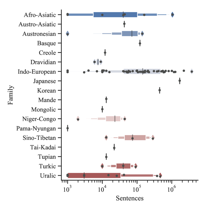
Figure 1: Annotated examples per family in the Universal Dependencies treebanks. Dots indicate individual languages, whereas boxes and whiskers mark quartiles.

We run experiments on Universal Dependencies (Zeman et al., 2020) for part-of-speech (POS) tagging and TyDiQA (Clark et al., 2020) for question answering (QA). We perform knowledge transfer to 14 and 8 target languages, respectively, which belong to under-represented and often endangered families (such as Tupian from Southern America and Pama–Nyugan from Australia). We report modest but consistent gains for the average performance across languages in few-shot and zero-shot learning settings and mixed results for the minimum performance. In particular, Minimax and Neyman–Pearson MAML often surpass vanilla MAML and multi-source transfer baselines, which are currently considered state-of-the-art in these tasks (Wu and Dredze, 2019; Ponti et al., 2021; Clark et al., 2020).

2 Skewed Language Distributions

Cross-lingual learning aims at transferring knowledge from resource-rich languages to resource-poor languages, to compensate for their deficiency of annotated data (Tiedemann, 2015; Ruder et al., 2019; Ponti et al., 2019a). The set of target languages ideally encompasses most of the world’s languages. However, the source languages available for training are often concentrated around few families, geographic areas, and typological features Cotterell and Eisner (2017); Gerz et al. (2018b, a); Ponti et al. (2020); Clark et al. (2020). As a consequence of this discrepancy, a language drawn at random might have no related languages available for training. Even when this is not the case, they might provide a scarce amount of examples for supervision.

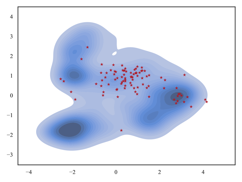
Figure 2: Density of WALS typological features of the world’s languages reduced to 2 dimensions via PCA. Red dots are languages covered by UD. Darkness corresponds to more probable regions.

To illustrate this point, consider Universal Dependencies (UD; Zeman et al., 2020), hitherto the most comprehensive collection of manually curated multilingual data. First, out of 245 families attested in the world according to Glottolog (Hammarström et al., 2016), UD covers only 18. In fact, some families are chronically over-represented (e.g. Indo-European and Uralic) and others are neglected (e.g. Pama-Nyugan and Uto-Aztecan). Second, as shown in Figure 1, the allocation of labelled examples across families is imbalanced (e.g. note the low counts for Niger–Congo or Dravidian languages). Third, one can measure how representative the linguistic traits of training languages are in comparison to those encountered around the globe. In Figure 2, we represent UD languages as dots in the space of possible typological features in WALS (Dryer and Haspelmath, 2013). These are plotted against the density of the distribution based on all languages in existence. Crucially, it emerges that UD languages mostly lie in a low-density region. Therefore, they hardly reflect the variety of possible combinations of typological features.

In general, this demonstrates that the distribution of training languages in existing NLP datasets is heavily skewed compared to the real-world distribution. Indeed, this very argument holds true a fortiori in smaller, less diverse datasets. While this fact is undisputed in the literature, its consequences for modelling, which we expound in the next section, are often under-estimated.

3 Robust MAML

Model-Agnostic Meta Learning (MAML; Finn et al., 2017) has recently emerged as an effective approach to cross-lingual transfer (Gu et al., 2018; Nooralahzadeh et al., 2020; Wu et al., 2020; Li et al., 2020). MAML seeks a good initialisation point for neural weights in order to adapt them to new languages with only a few examples. To this end, for each language $\mathcal{T}_{i}$ a neural model $f_{\boldsymbol{\vartheta}}$ is updated according to the loss on a batch of examples $\mathcal{L}_{\mathcal{T}_{i}}(f_{\boldsymbol{\vartheta}},\mathcal{D}_{train})$. This inner loop is iterated for k steps. Afterwards, the loss incurred by the model on a held-out batch $\mathcal{D}_{val}$ is compounded with those of the other languages as part of an outer loop, as shown in Equation 1:

$$\begin{split}{\boldsymbol{\vartheta}}^{\star}=\min_{\boldsymbol{\vartheta}}\sum_{\mathcal{T}_{i}}\mathcal{L}_{\mathcal{T}_{i}}(f_{{\boldsymbol{\varphi}}_{i}},\mathcal{D}_{val})\,p(\mathcal{T}_{i})\\ \text{where}\quad{\boldsymbol{\varphi}}_{i}={\boldsymbol{\vartheta}}-\eta\nabla_{\boldsymbol{\vartheta}}\mathcal{L}_{\mathcal{T}_{i}}(f_{\boldsymbol{\vartheta}},\mathcal{D}_{train})\end{split}$$ (1)

where $\eta\in\mathbb{R}_{>0}$ is the learning rate. Language probabilities are often taken to follow a discrete uniform distribution $p(\mathcal{T}_{i})=\frac{1}{|\mathcal{T}|}$. In this case, Equation 1 becomes a simple average.

MAML can also be interpreted as point estimate inference in a hierarchical Bayesian graphical model (see Figure 4 in the Appendix). In this case, the adapted parameters ${\boldsymbol{\varphi}}_{i}$ are equivalent to an intermediate language-specific variable acting as a bridge between the language-agnostic parameters ${\boldsymbol{\vartheta}}$ and the data (Grant et al., 2018; Finn et al., 2018; Yoon et al., 2018). This allows us to reason about the conditions under which a model is expected to generalise to new languages. Crucially, generalisation rests on the assumption of independence and identical distribution among the examples (including both train and evaluation), which is known as exchangeability (Zabell, 2005). However, as seen in Section 2, most of the world’s languages are outliers with respect to the training language distribution. Therefore, there is no solid guarantee that meta-learning may fulfil its purpose, i.e. generalise to held-out languages.

3.1 Decision-Theoretic Perspective

To remedy the mismatch between assumptions and realistic conditions, in this work we propose objectives which can serve as alternatives to Equation 1 of vanilla MAML. These are rooted in an interpretation of MAML within a decision-theoretic perspective (Bickel and Doksum, 2015, ch. 1.3), which we outline in what follows. The quantity of interest we aim at learning is the neural parameters ${\boldsymbol{\vartheta}}$. Therefore, the action space for a classification task assigning labels $y\in\mathcal{Y}$ to inputs $\mathbf{x}\in\mathcal{X}$ is $\mathcal{A}=\{f_{\boldsymbol{\vartheta}}:\mathcal{X}\rightarrow\mathcal{Y}\}$. The risk function is in turn a function $\mathcal{R}:\mathcal{F}\times\mathcal{A}\rightarrow\mathbb{R}^{+}$, which is the loss incurred by taking an action in $\mathcal{A}$ (making a prediction with a specific configuration of neural parameters) when the ‘state of nature’, the true function, is $f\in\mathcal{F}$. In the case of MAML, this is represented by the language-specific inner loop loss $\mathcal{L}_{\mathcal{T}_{i}}(\cdot)$ in Equation 1.

The decision for the optimal action given the sample space, the function $\delta:\mathcal{X}\times\mathcal{Y}\rightarrow\mathcal{A}$, is usually determined via gradient descent optimisation for a neural network. The optimal action, however, may vary depending on the language, which results in multiple possible ‘states of nature’. Usually, there is no procedure $\delta$ whose loss is inferior to all others, such that:

$$\nexists\delta\;\mathcal{L}(\mathcal{T}_{i},\delta)<\mathcal{L}(\mathcal{T}_{i},\delta^{\prime})\;\forall\mathcal{T}_{i}\in\mathcal{T},\delta\neq\delta^{\prime}$$ (2)

Therefore, decision functions have to be compared based on a global criterion rather than in a pair-wise fashion between languages. As previously anticipated, Equation 1 minimizes the expected risk across languages, for an arbitrary choice of prior $p(\mathcal{T})$. In decision theory, a decision $\delta^{\star}$ with this property is called Bayes criterion.

3.2 Alternative Criteria

There exist alternative criteria to the Bayes criterion that are more justified in a setting that entails transfer between non-i.i.d. domains. Rather than minimising the Bayes risk, in this work, we propose to adjust MAML to either minimise the maximum risk (minimax criterion) or to enforce constraints on the risk for a subset of languages (Neyman–Pearson criterion). This is likely to yield more robust predictions for languages that are outliers to the training distribution. As demonstrated in Section 2, this definition encompasses most of the world’s languages.

3.2.1 Minimax Criterion

Rather than the expected risk, the criterion could depend instead on the worst case scenario, i.e. the language for which the risk is maximum. This requires to select such a language with max. As an alternative to reinforcement learning (Zhang et al., 2020), to keep our model fully differentiable, we relax the operator by treating the choice of language as a categorical distribution $\mathcal{T}_{i}\sim\text{Cat}(\cdot\mid{\boldsymbol{\tau}})$. The parameters ${\boldsymbol{\tau}}\in[0,1]^{|\mathcal{T}|},\sum_{i}\tau_{i}=1$ consist of language probabilities and are learned in an adversarial fashion:

$$\min_{{\boldsymbol{\vartheta}}}\max_{\mathcal{T}_{i}\sim\text{Cat}(\cdot\mid{\boldsymbol{\tau}})}\mathcal{L}_{\mathcal{T}_{i}}(f_{{\boldsymbol{\vartheta}}-\eta\nabla_{\boldsymbol{\vartheta}}\mathcal{L}_{\mathcal{T}_{i}}(f_{\boldsymbol{\vartheta}},\mathcal{D}_{train})},\mathcal{D}_{val})$$ (3)

Equation 3 can be interpreted as a two-player game between us (the scientists) and nature. We pick an action ${\boldsymbol{\vartheta}}$. Then nature picks a language $\mathcal{T}_{i}\in p(\mathcal{T})$ for which the risk is maximum given our chosen action. Therefore, our goal becomes to minimise such risk.

3.2.2 Neyman–Pearson Criterion

As an alternative, we might consider minimising the expected risk, but subject to a guarantee that the risk does not exceed a certain threshold for a subset of languages. In practice, we may want to enforce a set of inequality constrains, so that we minimise Equation 1 subject to $\{\mathcal{L}_{\mathcal{T}_{i}}\leq r\;\forall\mathcal{T}_{i}\in\mathcal{C}\}$, where $r\in\mathbb{R}_{+}$ is a hyper-parameter. In general, $\mathcal{C}\subseteq\mathcal{T}$ can be any subset of the training languages; in practice, here we take $\mathcal{C}=\mathcal{T}$. Constrained optimisation is usually implemented through Lagrange multipliers, where we add as many new terms to the objective as we have constraints (Bishop, 2006, ch. 7):

$$\min_{{\boldsymbol{\vartheta}}}\max_{{\boldsymbol{\lambda}}} \sum_{\mathcal{T}_{i}}\frac{1}{|\mathcal{T}|}\mathcal{L}_{\mathcal{T}_{i}}+\sum_{\mathcal{T}_{i}}\lambda_{i}(\mathcal{L}_{\mathcal{T}_{i}}-r)$$

$$=\min_{{\boldsymbol{\vartheta}}}\max_{{\boldsymbol{\lambda}}} \sum_{\mathcal{T}_{i}}\left(\frac{1}{|\mathcal{T}|}+\lambda_{i}\right)\mathcal{L}_{\mathcal{T}_{i}}-\lambda_{i}r$$ (4)

where ${\boldsymbol{\lambda}}$ is a vector of non-negative Lagrange multipliers $\{\lambda_{i}\geq 0\quad\forall\lambda_{i}\in{\boldsymbol{\lambda}}\}$ to be learned together with the parameters ${\boldsymbol{\vartheta}}$, but adversarially.

Intuitively, if the risk for the estimated parameters ${\boldsymbol{\vartheta}}$ lies in the permissible range, the constraints should become inactive $\{\lambda_{i}=0\quad\forall\lambda_{i}\in{\boldsymbol{\lambda}}\}$, i.e. each Lagrange multiplier should go towards 0. Otherwise, the solution should be affected by the constraints, which should keep ${\boldsymbol{\vartheta}}$ from trespassing the boundary $\{\mathcal{L}({\boldsymbol{\vartheta}})_{\mathcal{T}_{i}}=r\quad\forall\mathcal{T}_{i}\in\mathcal{T}\}$. In gradient-based optimisation, this unfolds as follows: the gradient of each $\lambda_{i}$ depends uniquely on $(\mathcal{L}_{\mathcal{T}_{i}}-r)$. Due to being maximised, the value of each $\lambda_{i}$ increases when the corresponding risk is above the threshold, and shrinks otherwise. Incidentally, note that the Lagrangian multipliers at the critical point ${\boldsymbol{\vartheta}}^{\star}$ are equal to the negative rate of change of $r$, as $\frac{\partial\mathcal{R}({\boldsymbol{\vartheta}}^{\star})}{\partial r}=-{\boldsymbol{\lambda}}$. In other words, upon convergence $\lambda_{i}$ expresses how much we can decrease the risk in $\mathcal{T}_{i}$ as we increase the threshold.

Constrained Parameters

The additional variables ${\boldsymbol{\tau}}$ and ${\boldsymbol{\lambda}}$, contrary to the neural parameters, are constrained in the values they can take. In neural networks, there are two widespread approaches to coerce variables within a certain range, viz. reparametrisation and gradient projection (Beck and Teboulle, 2003). For simplicity’s sake, we opt for the former, which just requires us to learn unconstrained variables and scale them with the appropriate functions. Thus, we redefine the above-mentioned variables as ${\boldsymbol{\tau}}\triangleq\textrm{softmax}({\boldsymbol{\tau}}_{u})$ and ${\boldsymbol{\lambda}}\triangleq\textrm{softplus}({\boldsymbol{\lambda}}_{u})$.

4 Optimisation in 2-Player Games

Based on the formulation of Minimax MAML and Neyman–Pearson MAML in Section 3.2, both are evidently instances of two-player games. On one hand, the first agent minimises the risk with respect to ${\boldsymbol{\vartheta}}$; on the other, the second agent maximises the risk with respect to ${\boldsymbol{\tau}}$ (for minimax) or ${\boldsymbol{\lambda}}$ (for Neyman–Pearson). In other words, both optimise the same (empirical risk) function in Equation 3 or Section 3.2.2, respectively, but with opposite signs. However, the first term of Section 3.2.2 does not depend on ${\boldsymbol{\lambda}}$. Therefore, Minimax MAML is a zero-sum game, but not Neyman–Pearson MAML.

If the risk function were convex, the solution would be well-defined as the Nash equilibrium. But this is not the case for a non-linear function such as a deep neural network. Therefore, we resort to an approximate solution through optimisation. The simplest approach in this scenario is Gradient Descent Ascent (GDA), where the set of parameters of both players are optimised simultaneously through gradient descent for the first player and gradient ascent for the second player. With a slight abuse of notation, let us define $\mathcal{R}\triangleq\mathcal{R}({\boldsymbol{\vartheta}}_{t},{\boldsymbol{\alpha}}_{t})$, where ${\boldsymbol{\alpha}}_{t}$ stands for the adversarial parameters (${\boldsymbol{\tau}}_{t}$ for Minimax and ${\boldsymbol{\lambda}}_{t}$ for Neyman–Pearson) at time $t$. Then the update rule is:

$${\boldsymbol{\vartheta}}_{t+1} ={\boldsymbol{\vartheta}}_{t}-\eta\nabla_{\boldsymbol{\vartheta}}\mathcal{R}$$ (5)

$${\boldsymbol{\alpha}}_{t+1} ={\boldsymbol{\alpha}}_{t}+\eta\nabla_{\boldsymbol{\alpha}}\mathcal{R}$$ (6)

for a learning rate $\eta\in\mathbb{R}$. Equations 5 and 6 are equivalent to allowing each player to ignore the other’s move and act as if it will remain stationary. This naïve assumption often leads to divergence or sub-par solutions during optimisation (Schäfer and Anandkumar, 2019).

4.1 Symplectic Gradient Adjustment

To overcome the limitations of GDA, several independent works (Balduzzi et al., 2018; Letcher et al., 2019; Gemp and Mahadevan, 2018) proposed to correct Equations 5 and 6 with an additional term. This consists of a matrix-vector product between the mixed second-order derivatives ($\mathrm{D}_{{\boldsymbol{\vartheta}}{\boldsymbol{\alpha}}}^{2}\mathcal{R}$ and $\mathrm{D}_{{\boldsymbol{\alpha}}{\boldsymbol{\vartheta}}}^{2}\mathcal{R}$, respectively) and the gradient of the risk with respect to the adversarial parameters ($\nabla_{\boldsymbol{\alpha}}\mathcal{R}$ and $\nabla_{\boldsymbol{\vartheta}}\mathcal{R}$, respectively). The resulting optimisation algorithm, Symplectic Gradient Adjustment (SGA), updates parameters as follows:

$${\boldsymbol{\vartheta}}_{t+1} ={\boldsymbol{\vartheta}}_{t}-\eta\nabla_{\boldsymbol{\vartheta}}\mathcal{R}-\eta^{2}\mathrm{D}_{{\boldsymbol{\vartheta}}{\boldsymbol{\alpha}}}^{2}\mathcal{R}\;\nabla_{\boldsymbol{\alpha}}\mathcal{R}$$ (7)

$${\boldsymbol{\alpha}}_{t+1} ={\boldsymbol{\alpha}}_{t}+\eta\nabla_{\boldsymbol{\alpha}}\mathcal{R}-\eta^{2}\mathrm{D}_{{\boldsymbol{\alpha}}{\boldsymbol{\vartheta}}}^{2}\mathcal{R}\;\nabla_{\boldsymbol{\vartheta}}\mathcal{R}$$ (8)

Intuitively, the mixed second-order derivative represents the interaction between the players, and the adversarial gradient represents the opponent’s move if they follow the simple GDA strategy. Schäfer and Anandkumar (2019) cogently demonstrate how Equations 7 and 8 correspond to an approximation of the Nash equilibrium of a local bi-linear approximation (with quadratic regulariser) of the underlying game dynamics.

In practice, estimating the above-mentioned products is tedious because of their space and time complexity. Therefore, we resort to an approximation known as Hessian-vector product (Pearlmutter, 1994). For the third term of Equation 7:

$$\mathrm{D}^{2}_{{\boldsymbol{\vartheta}}{\boldsymbol{\alpha}}}\mathcal{R}({\boldsymbol{\vartheta}},{\boldsymbol{\alpha}})\nabla_{\boldsymbol{\alpha}}\mathcal{R}({\boldsymbol{\vartheta}},{\boldsymbol{\alpha}})$$

$$= \frac{\partial}{\partial h}\nabla_{\boldsymbol{\vartheta}}\mathcal{R}({\boldsymbol{\vartheta}},{\boldsymbol{\alpha}}+h\nabla_{\boldsymbol{\alpha}}\mathcal{R}({\boldsymbol{\vartheta}},{\boldsymbol{\alpha}}))\biggr{\rvert}_{h=0}$$ (9)

And similarly for the matrix product term in Equation 8, by swapping ${\boldsymbol{\vartheta}}$ and ${\boldsymbol{\alpha}}$ in Section 4.1.

4.2 Adaptive Learning Rate and Momentum

While SGA may provide a more appropriate optimisation framework for competitive games, it still lacks several defining features of optimisers that accelerate convergence, such as first-order momentum and adaptive learning rate (second-order momentum). Therefore, we modify the update rule in Equations 7 and 8 to include both of these. Our starting point is Adam (Kingma and Ba, 2015). The changes we apply are the following (also illustrated in Algorithm 1):

Algorithm 1 Adaptive Symplectic Gradient Adjustment (ASGA)

0:  $\eta\in\mathbb{R}_{+}$: Learning rate

0:  $\beta_{1},\beta_{2}\in[0,1)$: Decay rates

0:  ${\boldsymbol{\vartheta}}_{0},{\boldsymbol{\alpha}}_{0}$: Initial parameter values

0:  $\mathcal{R}\triangleq\mathcal{R}({\boldsymbol{\vartheta}}_{t-1},{\boldsymbol{\alpha}}_{t-1}):\mathbb{R}^{|{\boldsymbol{\vartheta}}|+|{\boldsymbol{\alpha}}|}\rightarrow\mathbb{R}$

1:  ${\boldsymbol{m}}_{0}\leftarrow{\boldsymbol{0}}$ Initialise first moments

2:  ${\boldsymbol{v}}_{0}\leftarrow{\boldsymbol{0}}$ Initialise second moments

3:  $t\leftarrow 0$ Initialise time step

4:  while ${\boldsymbol{\vartheta}}_{t},{\boldsymbol{\alpha}}_{t}$ not converged 

5:     $t\leftarrow t+1$

6:     ${\boldsymbol{g}}_{{\boldsymbol{\vartheta}},t}\leftarrow\nabla_{\boldsymbol{\vartheta}}\mathcal{R}{\color[rgb]{0.68359375,0.109375,0.15625}+\eta D_{{\boldsymbol{\vartheta}}{\boldsymbol{\alpha}}}\mathcal{R}\;\nabla_{\boldsymbol{\alpha}}\mathcal{R}}$

7:     ${\color[rgb]{0.12890625,0.2734375,0.546875}{\boldsymbol{g}}_{{\boldsymbol{\alpha}},t}\leftarrow\nabla_{\boldsymbol{\alpha}}\mathcal{R}}{\color[rgb]{0.68359375,0.109375,0.15625}-\eta D_{{\boldsymbol{\alpha}}{\boldsymbol{\vartheta}}}\mathcal{R}\;\nabla_{\boldsymbol{\vartheta}}\mathcal{R}}$

8:     ${\color[rgb]{0.12890625,0.2734375,0.546875}{\boldsymbol{g}}_{t}\leftarrow{\boldsymbol{g}}_{{\boldsymbol{\vartheta}},t}\oplus{\boldsymbol{g}}_{{\boldsymbol{\alpha}},t}}$

9:     ${\boldsymbol{m}}_{t}\leftarrow{\beta_{1}\,{\boldsymbol{m}}_{t-1}+(1-\beta_{1})\,{\boldsymbol{g}}_{t}}$

10:     ${\boldsymbol{v}}_{t}\leftarrow\beta_{2}\,{\boldsymbol{v}}_{t-1}+(1-\beta_{2})\,{\boldsymbol{g}}_{t}^{2}$

11:     ${\boldsymbol{\hat{m}}}_{t}\leftarrow{\boldsymbol{m}}_{t}\,/\,(1-\beta_{1}^{t})$

12:     ${\boldsymbol{\hat{v}}}_{t}\leftarrow{{\boldsymbol{v}}_{t}\,/\,(1-\beta_{2}^{t})}$

13:     ${\boldsymbol{\vartheta}}_{t}\leftarrow{\boldsymbol{\vartheta}}_{t-1}-\eta\cdot{\boldsymbol{\hat{m}}}_{{\boldsymbol{\vartheta}},t}\,/\,(\sqrt{{\boldsymbol{\hat{v}}}_{{\boldsymbol{\vartheta}},t}}+\epsilon)$

14:     ${\color[rgb]{0.12890625,0.2734375,0.546875}{\boldsymbol{\alpha}}_{t}\leftarrow{\boldsymbol{\alpha}}_{t-1}+\eta\cdot{\boldsymbol{\hat{m}}}_{{\boldsymbol{\alpha}},t}\,/\,(\sqrt{{\boldsymbol{\hat{v}}}_{{\boldsymbol{\alpha}},t}}+\epsilon)}$

15:  return  ${\boldsymbol{\vartheta}}_{t},{\boldsymbol{\alpha}}_{t}$

1. The current difference (lines 6–7) is adjusted with the terms introduced in Equations 7 and 8 by Schäfer and Anandkumar (2019).

2. The exponentially decayed, unbiased estimates of the expectations over mean and standard deviation are computed similarly to Adam. However, note that, in line 14, the update of the adversarial parameters corresponds to an ascent (rather than a descent).

This results in a novel optimiser, Adaptive Symplectic Gradient Adjustment (ASGA). We employ ASGA in our experiments to optimise the objectives of Minimax MAML and Neyman–Pearson MAML, as it enables a fair comparison with Adam-optimised Bayes MAML.

5 Experiments

We now outline the main experiments of our work on multilingual NLP. We evaluate our methods on part-of-speech (POS) tagging, a sequence labelling tasks, and question answering (QA), a natural language understanding task.

We focus on POS given its ample coverage of languages and its frequent use as a benchmark for resource-poor NLP (Das and Petrov, 2011; Ponti et al., 2021). In fact, cross-lingual transfer in sequence labelling tasks was demonstrated to be the most challenging, as knowledge of linguistic structure is more language-dependent than semantics (Hu et al., 2020). However, we also include QA to illustrate the generality of our methods for cross-lingual NLP. In this task, given the gold passage and a question, the system has to predict the beginning and end positions of a single contiguous span containing the answer.

Data. POS data are sourced from the Universal Dependencies (UD) treebanks Zeman et al. (2020) and QA data from the ‘gold passage’ variant of TyDiQA (Clark et al., 2020). We retain the original training, development, and evaluation sets of UD. In TyDiQA, we use the original development set for evaluation. For meta-learning, $\mathcal{D}_{train}$ and $\mathcal{D}_{val}$ examples are both obtained from disjoint parts of the training set.

We aim to create a partition of languages between training and evaluation that corresponds to the most realistic scenario in deploying NLP technology on resource-poor languages spoken around the world. Therefore, we reserve for evaluation all language isolates and languages with at most 2 family members in each dataset. We use all the remaining languages in the dataset for training. Therefore, for POS, the evaluation set spans 16 treebanks (14 languages, 11 families) and the training set 99 treebanks; QA comprises 9 languages (7 families). We hold out 4 of them in turn for evaluation (except English) and use the rest for training. We provide the full list of languages in Appendix A.

Training. In all tasks, we train a neural network consisting of two stacked modules: an encoder and a classifier. The encoder is a 12-layer, 768-hidden unit, 12-head Transformer initialised with multilingual BERT Base (mBERT), which was pre-trained on cased text from 104 languages. The classifier is a single affine layer for TyDiQA and a 2-layer Perceptron (with 1024 hidden units) for POS tagging. The combined parameters of the encoder and classifier correspond to ${\boldsymbol{\vartheta}}$ from Section 3.

These are meta-learned via Meta-SGD (Li et al., 2017), a first-order MAML variant where each parameter is assigned a separate inner-loop learning rate $\eta$. Moreover, each $\eta$ is trained end-to-end based on the outer-loop loss (such as Equation 1 for the Bayes criterion). Similar to Bansal et al. (2020), to avoid an explosion in the number of parameters, we assign a per-layer learning rate (rather than per-parameter). To avoid overfitting, we employ both dropout (with a probability of $0.2$) and early stopping (with a patience of $10$). For the Neyman-Pearson formulation, we set $r=0.1$ as a threshold for all language-specific losses. The parameters ${\boldsymbol{\tau}}$ and ${\boldsymbol{\lambda}}$ were initialized uniformly as $\frac{1}{|\mathcal{T}|}$. Complete details of the hyper-parameters for all settings are given in Appendix B.

Methods. To assess the effectiveness of the proposed criteria and optimisers, we compare them with two competitive baselines, while maintaining the same underlying neural architecture: (i) J: a joint multi-source transfer method where a model is trained on the concatenation of the datasets for all languages; (ii) B: the original MAML (Finn et al., 2017) with Bayes criterion and uniform prior. Our choice of baselines is justified by the fact that these methods (or variations thereof) are currently state of the art for the tasks of POS and QA, as well as other innumerable NLP applications (Wu and Dredze, 2019; Nooralahzadeh et al., 2020; Ponti et al., 2021). In addition, we evaluate the following combinations: (iii) MM: MAML with a minimax criterion, optimised with GDA; (iv) NP: MAML with a Neyman–Pearson (constrained) criterion, optimised with GDA; (v) MM+: MAML with a minimax criterion, optimised with ASGA; and (vi) NP+: MAML with a Neyman–Pearson criterion, optimised with ASGA.

Evaluation. For each evaluation language in a given task, we randomly sample $k\in\{0,5,10,20\}$ examples from the evaluation data as the support set (for adaptation) and the rest of the examples as the query set (for testing). When $k>0$, we repeat the evaluation 100 times and report the following average metrics: (i) F₁ score for POS tagging, and (ii) exact-match (EM) and F₁ scores for QA. Due to lack of space, we only report the average mean and standard deviation across languages for each model described above.

6 Results and Discussion

k $\triangleright$	0	5	10	20
F1 Score
J	51.01	62.96$\pm$2.5	66.00$\pm$1.9	68.66$\pm$1.7
B	51.50	63.87$\pm$2.8	67.03$\pm$2.1	69.46$\pm$1.8
MM	51.82	63.67$\pm$2.7	66.88$\pm$2.0	69.55$\pm$1.8
NP	51.68	63.84$\pm$2.9	67.13$\pm$2.1	69.65$\pm$1.9
MM+	52.46	64.71$\pm$2.9	67.89$\pm$2.3	70.25$\pm$2.0
NP+	53.05	64.26$\pm$2.6	67.57$\pm$2.1	69.98$\pm$1.9

Table 1: F₁ scores for POS tagging in UD across different k-shots. We report the mean and standard deviation across 16 treebanks.

k $\triangleright$	0	5	10	20
Exact Match
J	46.76	49.53$\pm$3.7	51.54$\pm$2.9	53.51$\pm$2.4
B	46.60	48.41$\pm$3.4	50.24$\pm$2.9	52.02$\pm$2.6
MM	48.33	50.08$\pm$3.4	51.68$\pm$2.9	53.49$\pm$2.4
NP	46.71	49.24$\pm$3.3	50.95$\pm$2.9	52.76$\pm$2.4
MM+	46.87	47.74$\pm$3.8	49.42$\pm$3.4	51.40$\pm$2.5
NP+	48.02	48.77$\pm$3.9	50.75$\pm$3.1	52.66$\pm$2.6
F1 Score
J	61.66	63.75$\pm$3.3	65.39$\pm$2.3	67.01$\pm$1.9
B	62.51	63.29$\pm$3.2	64.87$\pm$2.5	66.31$\pm$2.1
MM	63.06	64.37$\pm$3.1	65.83$\pm$2.6	67.45$\pm$2.1
NP	61.89	63.84$\pm$2.9	65.23$\pm$2.6	66.88$\pm$1.9
MM+	62.10	62.63$\pm$3.2	64.11$\pm$2.9	65.89$\pm$2.1
NP+	62.75	62.98$\pm$3.6	64.77$\pm$2.9	66.57$\pm$2.2

Table 2: Results for QA in TyDiQA across different k-shots. We report the mean and standard deviation across 8 languages of the exact match score (above) and the F₁ score (below).

We report the results for POS tagging in Table 1 and for QA in Table 2. These include mean and standard deviation across languages. Note that, in this case, the standard deviation is by no means an interval for statistical significance, but rather reflects the heterogeneity among the evaluation languages. In what follows, we address a series of questions in the light of these figures.

Baselines. MAML and joint multi-source transfer are both strong contenders as state-of-the-art methods for cross-lingual transfer, but which one is better? By comparing J and B rows, no definite response emerges in our experiments. While MAML outperforms its competitor in POS tagging, it lags behind in QA. We speculate that the larger pool of training languages available in POS tagging (22 times more than QA) endows meta-learning with better generalisation capabilities. Both methods, however, surpass single-source transfer from English SQuAD (Rajpurkar et al., 2016) in the zero-shot setting by a large margin: Clark et al. (2020) report 56.4 F₁ score in average for TyDiQA, which is 6.66 points below our best model.

Criteria. The minimax and Neyman-Pearson criteria both improve over the Bayes criterion baseline, although the latter more sporadically. Compared to the B rows, MM+ achieves gains for every k in POS tagging, with $0.94$ points of margin at $k=0$ and $0.79$ at $k=20$. The same holds for MM in QA, with margins that span from $1.73$ at $k=0$ to $1.47$ at $k=20$ in the Exact Match metric, and from $0.55$ at $k=0$ to $1.14$ at $k=20$ in F₁ score. Therefore, Minimax MAML is remarkably consistent in outperforming the baselines, although the gains are sometimes significant, sometimes only marginal. This is also reflected in language-specific performances, available in Table 5 and Table 6 in the Appendix. For POS tagging, the F₁ scores of only 2 languages (Indonesian and Naija) moderately decrease, whereas the rest of the 14 languages show improvements.

Incidentally, it may be worth noting that we did not perform any large-scale search over hyper-parameters like ${\boldsymbol{\tau}}$ and ${\boldsymbol{\lambda}}$ initialisations, the threshold $r$, or differential learning rates for maximised and minimised parameters. Therefore, these early results are amenable to improve even further in the future. This lends credence to our proposition that minimax and Neyman–Pearson criteria are more suited for out-of-distribution transfer to outlier languages.

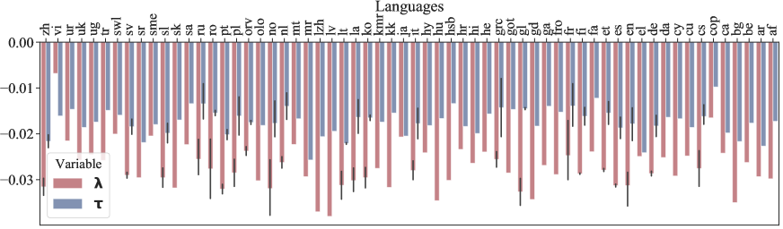
Figure 3: Unconstrained values of ${\boldsymbol{\tau}}_{u}$ and ${\boldsymbol{\lambda}}_{u}$ upon convergence in MM+ and NP+ models for POS tagging.

k $\triangleright$	0	5	10	20
F1 Score
J	14.34	33.32	37.52	40.83
B	24.11	35.03	40.38	44.92
MM	20.41	37.61	43.00	45.83
NP	26.81	39.23	42.70	45.25
MM+	16.42	37.41	43.57	45.21
NP+	22.55	39.95	45.41	48.12

Table 3: The minimum F₁ scores of our models across languages, for POS tagging.

k $\triangleright$	0	5	10	20
Exact Match
J	42.33	45.97	47.22	49.47
B	42.75	44.58	46.44	48.24
MM	41.01	45.33	47.59	49.21
NP	40.39	44.89	46.40	48.80
MM+	41.01	41.87	45.32	47.11
NP+	37.44	42.92	46.30	48.88
F1 Score
J	52.43	59.27	59.88	62.11
B	51.10	59.60	60.64	62.10
MM	53.10	59.21	61.86	63.43
NP	52.83	59.31	60.03	61.84
MM+	51.93	57.91	59.86	61.52
NP+	53.96	57.21	61.74	63.55

Table 4: The minimum Exact Match and F₁ scores of our models across languages, for QA.

Optimiser. The results for the proposed optimiser ASGA (Algorithm 1) are favourable in comparison to Gradient Descent Ascent via Adam (Kingma and Ba, 2015) for POS tagging; on the other hand, the opposite trend is observed for QA. Therefore, future investigations are required to shed further light on modifications such as the Symplectic Gradient Adjustment. A tentative explanation of such discrepancy could be the disproportionate number of training languages available in either task.

To get insights into the game dynamics of the adversarial criteria, we plot the unconstrained values for ${\boldsymbol{\tau}}_{u}$ and ${\boldsymbol{\lambda}}_{u}$ upon convergence in Figure 3. Interestingly, both variables appear to follow the same profile of peaks and troughs; therefore, as expected, languages chosen adversarially in MM have also higher Laplace multipliers in NP. To this group belong for instance languages with rare scripts (e.g. Coptic) or with no relatives in the training languages (e.g. Vietnamese). As a final note, we remark that the proposed criteria and optimiser are in principle more general than NLP and could facilitate transfer in other fields. While this thread of research transcends the scope of our work, we illustrate an example for regression in Appendix C.

Minimum Scores across Languages. In addition to the average cross-lingual performance, we also report the minimum cross-lingual performance for POS tagging in Table 3 and for QA in Table 4. This corresponds to the lowest score achieved across all evaluation languages. For POS tagging, we observe that NP and NP+ outperform J and B by 7-12 and 2-5 F1 points, respectively. This reveals that worst-case and constrained risk minimisation drastically uplifts the scores for the most disadvantaged language. Nevertheless, the opposite trend is observed for QA: MM(+) and NP(+) do not alter the minimum score with respect to the F₁ metric, and even degrade it with respect to the exact-match metric. Again, we conjecture that these mixed findings may depend on the different amount and distribution of the training languages in the corresponding datasets: UD offers greater language coverage than TyDiQA, which gives better guidance.

7 Related Work

MAML is a cutting-edge method for cross-lingual transfer in several NLP tasks (Gu et al., 2018; Nooralahzadeh et al., 2020; Wu et al., 2020; Li et al., 2020, inter alia). However, in all these experiments, the model is adopted in its standard formulation, minimising the expected risk. Therefore, its performance is prone to suffer in outlier languages. Moreover, the assumptions underlying our proposed variants are different from other instances of robust optimisation in NLP Globerson and Roweis (2006); Oren et al. (2019). In particular, the target language distributions are not explicitly treated as subspaces or covariate shifts of source languages. In separate fields such as vision, previous attempts at worst-case-aware meta-learning include Collins et al. (2020), who use a Euclidean version of the robust stochastic mirror-prox algorithm, and Wang et al. (2020), who rely on reinforcement learning. Our formulation is both fully differentiable and broader, as the decision-theoretic interpretation admits alternative criteria for MAML. What is more, to our knowledge we are the first to successfully augment MAML with minimax criteria in cross-lingual NLP and with Neyman–Pearson criteria in general.

8 Conclusions

To perform cross-lingual transfer to low-resource languages, under a decision-theoretic interpretation Model-Agnostic Meta-Learning (MAML) minimises the expected risk across training languages. Generalisation then relies on the evaluation languages being identically distributed. However, this assumption is incongruous for cross-lingual transfer in realistic scenarios. Therefore, we propose more appropriate training objectives that are robust to out-of-distribution transfer: Minimax MAML, where worst-case risk is minimised by learning an adversarial distribution over languages; and Neyman–Pearson MAML, where constraints are imposed on language-specific losses, so that they remain below a certain threshold. From a game-theoretic perspective, both of these variants consist of 2-player competitive games. Therefore, we also explore adaptive optimisers that take into account the underlying game dynamics. The experimental results on zero-shot and few-shot learning for part-of-speech tagging and question answering, whose datasets span tens of typologically diverse languages, confirm that in several settings the proposed criteria are superior to both vanilla MAML and transfer from multiple source languages.

Figure 4: Bayesian graphical model of MAML, where the variable ${\boldsymbol{\varphi}}_{i}$ is parameterised as ${\boldsymbol{\vartheta}}-\eta\nabla_{\boldsymbol{\vartheta}}\mathcal{L}_{\mathcal{T}_{i}}(f_{\boldsymbol{\vartheta}},\mathcal{D}_{train})$.

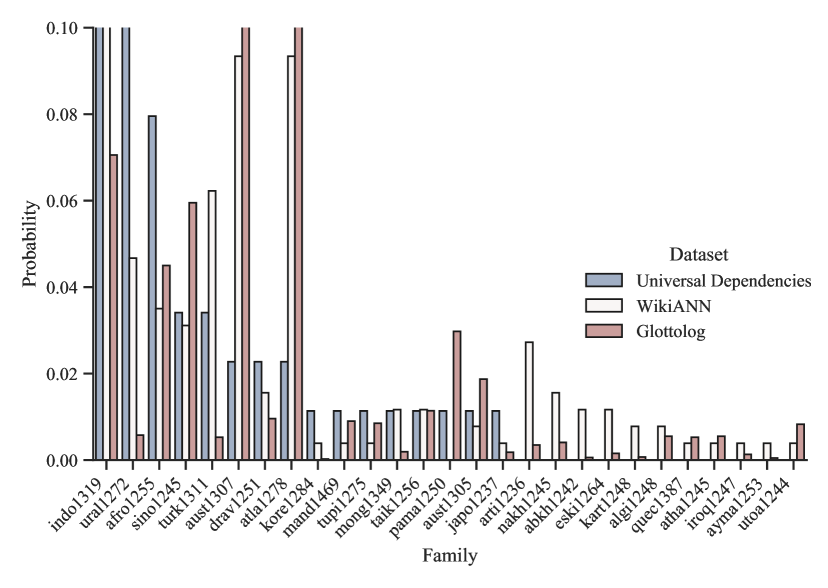
Figure 5: Empirical distribution of languages across families in 2 datasets (WikiANN and UD) and in the world, according to Glottolog. The families shown are a subset {(WikiANN $\cup$ Universal Dependencies) $\cap$ Glottolog}. The y-axis is truncated for the sake of clarity.

Appendix A Language Partitions

The languages from the following families in UD are held out for evaluation (16 treebanks, 14 languages in total): Northwest Caucasian (Abaza), Mande (Bambara), Mongolic (Buryat), Basque, Tupian (Mbya Guarani), Creole (Naija), Tai–Kadai (Thai), Pama–Nyungan (Warlpiri), Austronesian (Indonesian, Tagalog), Dravidian (Tamil, Telugu), Niger-Congo (Wolof, Yoruba). As all 8 languages in TiDiQA belong to families with at most 2 members in the dataset, we randomly create two partitions: in the former, Finnish, Korean, Bengali, and Arabic are used for evaluation, and the others for training; in the latter, Russian, Indonesian, Telugu, and Swahili are used for evaluation, and the others for training.

Appendix B Hyperparameter Setting

POS Tagging.

For POS tagging: (i) the batch size was $32$, (ii) the maximum sequence length was $128$, (iii) the number of epochs was $20$, with a patience limit of $10$, (iv) both outer and inner learning rates were $5\times 10^{-5}$, (v) the number of episodes per iteration was $32$, (vi) the number of inner loops per outer update was $4$, (vii) the number of shots ($k$) during training was $30$, and (viii) the hidden layer dropout probability for the classifier was $0.2$.

QA.

(i) the batch size and $k$ were reduced to $12$ due to memory constraints, (ii) the maximum context length was $336$, and the document stride was $128$, (iii) the maximum question length was $64$, (iv) the inner and outer learning rates were $3\times 10^{-5}$.

For all J baselines, we used a uniform language sampler, since proportional sampling performed worse. As an optimiser, we chose Adam with a learning rate of $5\times 10^{-5}$, a weight decay of $0.1$; we clipped the gradient to a maximum norm of $5.0$. For all MAML models, we performed 4 updates in the inner loop, both during training and fast adaptation (few-shot learning). We ran our experiments on a 48GB NVIDIA Quadro RTX 8000 GPU with Turing micro-architecture. Each run took approximately 2 hours for training and 3 hours for few-shot learning and evaluation.

Dataset	k	J	B	MM	NP	MM+	NP+
abq_atb	0	14.34	24.11	20.41	26.81	16.42	22.55
	5	33.32$\pm$5.58	35.03$\pm$5.85	37.61$\pm$4.57	39.23$\pm$5.41	37.41$\pm$7.3	39.95$\pm$5.93
	10	37.52$\pm$2.28	40.38$\pm$5.75	43$\pm$3.63	42.7$\pm$5.3	43.57$\pm$7.31	46.56$\pm$4.91
	20	40.83$\pm$6.53	44.92$\pm$7.08	45.83$\pm$5.59	45.25$\pm$7.26	45.21$\pm$9.4	48.12$\pm$7.19
bm_crb	0	29.56	30.85	29.2	28.57	30.44	30.22
	5	45.6$\pm$3.47	50.83$\pm$3.33	46.04$\pm$3.95	45.14$\pm$3.73	48.2$\pm$3.74	48.32$\pm$3.63
	10	49.75$\pm$1.23	54.4$\pm$2.73	50.35$\pm$2.7	50.01$\pm$2.74	51.65$\pm$2.87	51.28$\pm$3.4
	20	54.03$\pm$1.52	57.53$\pm$1.68	53.12$\pm$2.16	53.39$\pm$1.85	54.38$\pm$1.85	53.89$\pm$2.08
bxr_bdt	0	48.85	51.71	50.41	50.49	54.21	51.94
	5	51.29$\pm$1.67	51.81$\pm$2.18	51.57$\pm$2.21	51.62$\pm$2.17	53.09$\pm$2.08	51.83$\pm$2.31
	10	53.64$\pm$0.96	54.95$\pm$1.68	54.18$\pm$1.53	54.25$\pm$1.63	55.47$\pm$1.8	55.17$\pm$1.43
	20	56.18$\pm$1.13	57.23$\pm$1.17	56.48$\pm$1.49	56.97$\pm$1.2	58.19$\pm$1.38	57.29$\pm$1.12
eu_bdt	0	70.2	71.76	73.22	72.57	73.54	73.29
	5	74.7$\pm$1.39	75.74$\pm$1.69	75.42$\pm$1.59	75.77$\pm$1.94	76.58$\pm$1.64	76.52$\pm$1.64
	10	76.51$\pm$2.38	78.1$\pm$1.25	77.52$\pm$1.01	78.08$\pm$1.21	78.73$\pm$1.36	78.19$\pm$1.38
	20	78.52$\pm$0.67	80.09$\pm$0.87	79.47$\pm$0.84	80.01$\pm$0.76	80.69$\pm$0.91	80.24$\pm$0.78
gun_thomas	0	32.06	35.72	33.91	31.97	33.87	33.84
	5	40.65$\pm$2.27	42.62$\pm$3.05	43.28$\pm$2.64	42.32$\pm$2.45	43.12$\pm$2.63	42.46$\pm$2.37
	10	44.06$\pm$0.99	45.65$\pm$2.33	45.92$\pm$2.59	45.23$\pm$2.31	46.98$\pm$2.49	45.41$\pm$2.25
	20	46.46$\pm$2.07	47.96$\pm$2.11	50.34$\pm$2.3	48.15$\pm$2.09	50.67$\pm$2.15	48.44$\pm$1.74
id_gsd	0	77.24	77.97	77.68	74.79	77.85	76.15
	5	82.2$\pm$1.22	83.47$\pm$1.22	82.72$\pm$1.47	82.35$\pm$1.68	83$\pm$1.5	82.47$\pm$1.57
	10	83.63$\pm$0.93	84.69$\pm$0.91	84.28$\pm$1.17	84.06$\pm$1.09	84.4$\pm$1.03	84.69$\pm$0.96
	20	84.75$\pm$0.61	85.75$\pm$0.59	85.82$\pm$0.58	85.35$\pm$0.68	85.94$\pm$0.66	85.86$\pm$0.69
id_pud	0	68.46	69.41	69.27	68.67	69.41	68.72
	5	73.07$\pm$1.39	73.96$\pm$1.5	73.5$\pm$1.48	74.17$\pm$1.43	74.52$\pm$1.46	73.82$\pm$1.56
	10	74.91$\pm$1.33	75.7$\pm$1.19	75.5$\pm$1.08	75.87$\pm$1.15	76.42$\pm$0.8	75.85$\pm$0.94
	20	76.17$\pm$0.57	77.18$\pm$0.72	77.06$\pm$0.49	77.28$\pm$0.68	77.75$\pm$0.57	77.39$\pm$0.71
pcm_nsc	0	61.97	40.78	45.77	40.76	41.21	56.83
	5	78.17$\pm$1.58	77.87$\pm$1.27	77.42$\pm$1.67	76.48$\pm$1.74	77.33$\pm$1.55	77.71$\pm$1.78
	10	80.06$\pm$1.24	79.28$\pm$1.25	78.96$\pm$1.1	78.41$\pm$1.1	78.71$\pm$0.94	80.03$\pm$1.37
	20	81.61$\pm$0.85	80.6$\pm$0.81	80.17$\pm$0.8	79.97$\pm$1	80.13$\pm$0.72	81.99$\pm$0.99
ta_ttb	0	55.65	56.31	58.12	58.47	60.18	55.93
	5	72.29$\pm$2.03	72.39$\pm$2.21	71.37$\pm$1.7	72.28$\pm$2.46	72.34$\pm$2.13	70.19$\pm$2.3
	10	74.73$\pm$2.27	75.36$\pm$1.47	73.7$\pm$1.36	75.51$\pm$1.54	75.11$\pm$1.47	73.69$\pm$1.73
	20	76.23$\pm$1.19	77.56$\pm$1.38	75.75$\pm$1.39	77.83$\pm$1.33	77.44$\pm$1.3	76.29$\pm$1.49
te_mtg	0	75.21	75.87	77.49	75.43	76.28	76.29
	5	76.45$\pm$2.57	73.9$\pm$3.87	75.32$\pm$2.9	74.74$\pm$3.63	74.97$\pm$2.87	74.37$\pm$3.46
	10	78.68$\pm$1.74	77.16$\pm$2.55	78.26$\pm$2.09	77.55$\pm$2.29	77.57$\pm$2.12	76.94$\pm$2.83
	20	80.13$\pm$1.97	79.66$\pm$1.64	79.99$\pm$2.15	80$\pm$2.22	80.09$\pm$1.98	80.08$\pm$1.99
th_pud	0	42.51	42.71	43.76	43.3	46.81	43.07
	5	58.05$\pm$2.53	59.83$\pm$2.35	60.02$\pm$2.62	61.18$\pm$2.74	61.12$\pm$2.95	60.15$\pm$2.05
	10	61.71$\pm$2.17	63.57$\pm$1.72	63.85$\pm$1.9	65.14$\pm$1.67	65.4$\pm$1.87	63.34$\pm$1.75
	20	65.05$\pm$1.28	66.39$\pm$1.38	66.62$\pm$1.08	67.99$\pm$1.41	68.72$\pm$1.28	66.27$\pm$1.36
tl_trg	0	76.9	77.43	77.59	85.12	82.27	80.62
	5	83.01$\pm$3.52	82.95$\pm$3.66	84.09$\pm$4.75	84.5$\pm$4.14	84.4$\pm$4.01	84.01$\pm$4.64
	10	85.78$\pm$1.66	85.4$\pm$2.06	86.86$\pm$2.3	87.27$\pm$2.62	87.23$\pm$2.87	87.42$\pm$2.12
	20	87.27$\pm$2.04	87.48$\pm$2.32	88.69$\pm$1.96	89.1$\pm$2.34	89.2$\pm$1.85	89.24$\pm$1.86
tl_ugnayan	0	60.37	64.38	63.58	63.01	64.41	64.76
	5	74.8$\pm$1.86	76.35$\pm$2.27	75.73$\pm$2.01	75.2$\pm$2.37	78.13$\pm$2.01	76.91$\pm$2.44
	10	77.02$\pm$3.68	79.31$\pm$1.48	78.35$\pm$1.64	78.93$\pm$1.3	80.69$\pm$1.71	79.28$\pm$1.62
	20	78.91$\pm$1.44	82$\pm$1.07	80.86$\pm$1.04	81.14$\pm$1.32	82.66$\pm$1	81.71$\pm$1.31
wbp_ufal	0	26.64	24.55	28.62	27.21	27.96	30.18
	5	58$\pm$4.23	56.83$\pm$4.94	57.07$\pm$4.67	58.52$\pm$4.98	59.13$\pm$4.86	59.68$\pm$6.1
	10	64.72$\pm$1.72	63.34$\pm$4.41	64.51$\pm$3.43	65.94$\pm$3.88	65.2$\pm$4.03	66.32$\pm$3.63
	20	71.84$\pm$3.39	66.67$\pm$3.67	70.45$\pm$3.46	70.6$\pm$3.29	67.98$\pm$3.77	70.75$\pm$3.55
wo_wtb	0	34.79	33.05	34.72	34.11	34.09	35.27
	5	46.12$\pm$2.41	45.47$\pm$2.7	45.86$\pm$2.36	46.69$\pm$2.23	47.49$\pm$2.66	46.49$\pm$2.3
	10	50.01$\pm$2.03	48.49$\pm$1.69	49.13$\pm$2.18	49.69$\pm$1.79	50.97$\pm$2.1	49.67$\pm$2.1
	20	53.32$\pm$1.19	51.27$\pm$1.39	52.73$\pm$1.65	52.79$\pm$1.15	53.97$\pm$1.45	52.58$\pm$1.55
yo_ytb	0	41.46	47.34	45.31	45.59	50.45	49.1
	5	59.59$\pm$3.02	62.93$\pm$2.71	61.66$\pm$2.54	61.26$\pm$2.8	64.5$\pm$2.51	63.3$\pm$3.09
	10	63.34$\pm$	66.71$\pm$1.63	65.68$\pm$2	65.39$\pm$2.17	68.18$\pm$1.63	67.31$\pm$1.5
	20	67.23$\pm$1.06	69.14$\pm$1.19	69.45$\pm$1.01	68.56$\pm$1.43	70.9$\pm$1.1	69.58$\pm$1.25

Table 5: POS tagging results on all evaluation languages.

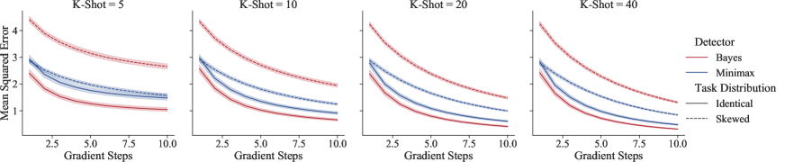
Figure 6: Mean Squared Error of MAML across gradient steps (from 1 to 10) of different criteria (B and MM) under identical and skewed task distributions. Each frame represents a separate run of fast adaptation with different amounts of target examples available ($k$-shot).

author=RA,color=yellow!20,size=,fancyline,caption=,]Neyman-Pearson curves missing in Figure 3.

Appendix C Additional Experiments & Results

Additional Results.

Table 5 contains POS tagging F₁ scores of all languages, for all models, in both zero and few-shot settings. Table 6 shows the exact match and F₁ scores for QA.

Sinusoidal Regression.

After delving into real-world, large-scale NLP applications, we additionally illustrate the effect of the alternative criteria on other ML domains. We run a proof-of-concept experiment on a toy task where we can fully control the distribution of the training and evaluation data, viz. regression of a sinusoidal function.

For this task, we follow the same experimental setting and hyper-parameters of Finn et al. (2017): combinations of amplitudes $a\in[0.1,5]$ and phases $p\in[0,\pi]$ determine a set of tasks characterised by the function $y=\sin(x-p)\cdot a$. The inputs are sampled at random from the interval $x\in[-5,5]$.

While both train and evaluation tasks in the original version were sampled uniformly from identical ranges, we also construct an alternative setting with skewed distributions sampled from disjoint ranges: during training, $a\in[2.5,5]$ and $p\in[\frac{\pi}{2},\pi]$; during evaluation, $a\in[0.1,2.5]$ and $p\in[0,\frac{\pi}{2}]$.

For Minimax MAML, we aim at learning the distribution over tasks adversarially. In particular, we consider two separate discrete categorical distributions for amplitudes $\mathrm{softmax}({\boldsymbol{\tau}}_{u}^{(a)})$ and phases $\mathrm{softmax}({\boldsymbol{\tau}}_{u}^{(p)})$ over their respective ranges discretised into 1,000 atoms. Hence, the probability of a task with the $i$-th amplitude value and the $j$-th phase value is simply $\tau_{i}^{(a)}\times\tau_{j}^{(p)}$.

The results for sinusoidal regression are shown in Figure 6. Vanilla MAML (Bayes criterion) consistently outperforms the minimax criterion when the task distribution is identical; on the other hand, the reverse occurs when the task distribution is skewed. MM performs much better in this case, with the gap in performance increasing as the shots $k$ decrease. This verifies our hypothesis that the minimax criterion should benefit out-of-distribution regression tasks.

Dataset	k	J	B	MM	NP	MM+	NP+
Exact Match
Arabic	0	48.97	49.29	51.47	51.36	49.4	48.64
	5	52.2$\pm$3.92	50.19$\pm$3.52	53.38$\pm$3.52	51.48$\pm$3.2	49.27$\pm$3.89	51.27$\pm$4.75
	10	54.51$\pm$2.47	52.81$\pm$2.93	54.96$\pm$2.93	53.67$\pm$2.16	52.05$\pm$3.27	53.67$\pm$3.43
	20	56$\pm$1.85	54.64$\pm$1.86	56.59$\pm$1.56	55.43$\pm$1.86	54.45$\pm$1.94	55.78$\pm$2.13
Bengali	0	45.13	46.02	51.33	44.25	45.13	51.33
	5	46.32$\pm$3.48	45.3$\pm$3.11	50.76$\pm$3.03	47.22$\pm$3.3	45$\pm$2.98	49.45$\pm$3.17
	10	47.22$\pm$3.15	46.44$\pm$3.08	50.83$\pm$2.94	49.39$\pm$3.84	45.98$\pm$3.7	50.01$\pm$3.22
	20	49.47$\pm$3.54	48.24$\pm$4.15	52.37$\pm$3.57	50.21$\pm$3.62	47.68$\pm$3.31	51.24$\pm$3.03
Finnish	0	42.33	43.61	47.95	49.36	47.83	46.42
	5	46.5$\pm$4.96	45.75$\pm$3.21	47.69$\pm$3.48	48.75$\pm$3.21	45.66$\pm$3.53	47.57$\pm$4.21
	10	48.56$\pm$2.65	47.25$\pm$2.81	49.43$\pm$2.78	50.28$\pm$3.1	46.85$\pm$2.77	48.55$\pm$3.1
	20	49.81$\pm$2.09	48.82$\pm$2.77	50.43$\pm$2.34	52.22$\pm$3.01	48.18$\pm$2.48	50.89$\pm$2.49
Korean	0	50	50.72	53.62	48.55	51.45	53.62
	5	51.37$\pm$2.52	49.5$\pm$2.76	51.87$\pm$2.11	49.52$\pm$2.48	49.57$\pm$2.35	52.17$\pm$2
	10	52.63$\pm$2.41	50.63$\pm$2.46	52.29$\pm$1.85	50.1$\pm$2.29	50.29$\pm$2.51	53$\pm$1.93
	20	54.07$\pm$2.11	51.88$\pm$2.15	53.55$\pm$1.91	51.87$\pm$2.03	51.71$\pm$2.13	53.67$\pm$2.16
Indonesian	0	56.46	51.86	54.87	56.28	52.74	56.28
	5	57.99$\pm$2.94	55.49$\pm$3.18	56.04$\pm$2.99	57.61$\pm$2.7	55.53$\pm$3.82	55.39$\pm$2.67
	10	59.4$\pm$2.49	57.11$\pm$2.81	58.54$\pm$2.49	58.59$\pm$1.96	57.08$\pm$2.84	56.86$\pm$1.95
	20	60.99$\pm$2.09	58.99$\pm$2.51	60.76$\pm$2.21	59.9$\pm$1.69	59.11$\pm$2.07	57.95$\pm$1.94
Russian	0	44.21	43.23	41.01	40.39	41.01	37.44
	5	49.45$\pm$4.36	47.41$\pm$3.92	46.66$\pm$4.01	46.83$\pm$4.34	46.2$\pm$4.61	44.09$\pm$5.38
	10	51.84$\pm$3.04	49.66$\pm$2.83	48.72$\pm$3.56	48.81$\pm$3.79	47.97$\pm$4.43	47.66$\pm$4.05
	20	53.6$\pm$2.45	50.72$\pm$2.55	51.05$\pm$2.8	51.5$\pm$2.75	50.47$\pm$2.45	50.25$\pm$2.96
Swahili	0	43.49	45.29	41.88	41.48	45.69	45.29
	5	46.47$\pm$5.11	49.07$\pm$4.31	48.9$\pm$4.88	47.6$\pm$4.21	48.8$\pm$4.28	47.32$\pm$4.3
	10	50.06$\pm$4.13	51.37$\pm$3.45	51.1$\pm$3.83	50.37$\pm$3.72	49.79$\pm$3.59	49.96$\pm$3.88
	20	54.02$\pm$3.06	53.82$\pm$2.63	53.94$\pm$2.54	52.16$\pm$2.89	52.51$\pm$3.47	52.65$\pm$3.26
Telugu	0	43.5	42.75	44.54	42	41.7	45.14
	5	45.97$\pm$2.85	44.58$\pm$3.44	45.33$\pm$3.91	44.89$\pm$3.44	41.87$\pm$5.35	42.92$\pm$5.36
	10	48.11$\pm$3.4	46.64$\pm$3.1	47.59$\pm$2.95	46.4$\pm$2.69	45.32$\pm$4.23	46.3$\pm$3.51
	20	50.1$\pm$2.55	49.08$\pm$2.42	49.21$\pm$2.77	48.8$\pm$1.97	47.11$\pm$2.71	48.88$\pm$2.91
F1 score
Arabic	0	65.57	67.38	66.59	67.44	64.98	65.45
	5	68.4$\pm$3.82	67.09$\pm$3.51	69.66$\pm$3.45	67.59$\pm$3.26	65.92$\pm$3.93	67.76$\pm$4.86
	10	70.56$\pm$2.47	69.55$\pm$2.88	71.35$\pm$2.83	69.82$\pm$2.15	68.82$\pm$3.64	70.28$\pm$3.63
	20	72.14$\pm$1.78	71.14$\pm$1.87	73.21$\pm$1.46	71.55$\pm$1.88	71.5$\pm$1.99	72.26$\pm$2.31
Bengali	0	57.24	62.57	66.29	59.64	60.28	62.86
	5	59.27$\pm$2.79	60.04$\pm$2.97	64.65$\pm$2.84	61.71$\pm$3.1	59.46$\pm$2.72	61.85$\pm$2.65
	10	59.88$\pm$2.7	60.64$\pm$2.86	64.88$\pm$2.71	63.52$\pm$3.38	60.03$\pm$3.28	62.33$\pm$2.89
	20	62.11$\pm$3.15	62.1$\pm$3.51	65.93$\pm$3.07	64.31$\pm$2.95	61.72$\pm$2.96	63.86$\pm$2.72
Finnish	0	61.85	63.57	61.72	63.79	62.12	61.64
	5	61.48$\pm$3.47	61.76$\pm$2.63	61.66$\pm$2.84	62.66$\pm$2.8	60.49$\pm$2.42	61.57$\pm$3.94
	10	62.98$\pm$1.53	62.48$\pm$2.03	63.26$\pm$2.31	64.14$\pm$2.7	61.58$\pm$2.15	62.58$\pm$2.91
	20	63.81$\pm$1.57	63.66$\pm$2.07	64.65$\pm$2.2	65.64$\pm$2.84	63$\pm$2.24	64.9$\pm$2.27
Korean	0	60.26	62.71	62.4	58.68	61.2	64.35
	5	61.31$\pm$2.47	60.82$\pm$2.47	61.67$\pm$2.17	59.31$\pm$2.34	59.27$\pm$2.33	62.13$\pm$2.01
	10	62.52$\pm$2.26	62.02$\pm$2.1	61.86$\pm$2.05	60.03$\pm$2.15	59.86$\pm$2.51	62.92$\pm$1.91
	20	64.04$\pm$2.01	63.08$\pm$1.87	63.43$\pm$1.89	61.84$\pm$1.97	61.52$\pm$1.89	63.55$\pm$1.95
Indonesian	0	69.96	65.99	70.05	70.82	68.02	70.19
	5	71.4$\pm$2.81	69.22$\pm$3.28	70.61$\pm$2.74	71.18$\pm$2.17	69.95$\pm$3.4	69.37$\pm$2.58
	10	72.69$\pm$2.27	70.79$\pm$2.78	72.79$\pm$2.53	72.23$\pm$1.77	71.33$\pm$2.46	70.93$\pm$1.96
	20	74.11$\pm$1.79	72.49$\pm$2.57	74.65$\pm$2.11	73.52$\pm$1.45	73.11$\pm$1.8	71.96$\pm$1.94
Russian	0	65.93	64.15	64.47	63.2	64.13	61.08
	5	66.96$\pm$1.52	65.11$\pm$1.5	65.03$\pm$1.39	65.13$\pm$1.33	64.58$\pm$1.45	62.17$\pm$1.61
	10	67.86$\pm$1.15	66.21$\pm$1.28	65.84$\pm$1.65	65.89$\pm$1.33	65.53$\pm$1.46	63.63$\pm$1.67
	20	68.7$\pm$1.01	66.85$\pm$1.38	66.94$\pm$1.45	67.1$\pm$1.38	66.4$\pm$1.19	65.01$\pm$1.82
Swahili	0	60.01	62.63	59.84	58.74	64.13	62.48
	5	60.21$\pm$4.38	62.7$\pm$3.37	62.48$\pm$3.72	61.9$\pm$3.41	63.43$\pm$3.38	61.81$\pm$4.06
	10	62.62$\pm$2.66	64.36$\pm$2.31	63.79$\pm$3.19	63.6$\pm$3.02	63.77$\pm$2.88	63.78$\pm$3.06
	20	65.18$\pm$2.09	65.89$\pm$2	66.27$\pm$1.99	65.48$\pm$1.7	66.21$\pm$2.19	66.12$\pm$2.11
Telugu	0	52.43	51.1	53.1	52.83	51.93	53.96
	5	60.99$\pm$5.15	59.6$\pm$6.05	59.21$\pm$6.17	61.27$\pm$5.05	57.91$\pm$6.64	57.21$\pm$7.33
	10	63.99$\pm$3.92	62.92$\pm$4.19	62.85$\pm$3.62	62.63$\pm$4.98	61.92$\pm$5.1	61.74$\pm$5.18
	20	65.96$\pm$2.37	65.29$\pm$2.15	64.53$\pm$3.06	65.63$\pm$1.61	63.67$\pm$2.58	64.9$\pm$3.26

Table 6: QA results on all evaluation languages.

References

- Arnold et al. (2020) Sébastien M. R. Arnold, Praateek Mahajan, Debajyoti Datta, Ian Bunner, and Konstantinos Saitas Zarkias. 2020. learn2learn: A library for meta-learning research. arXiv preprint arXiv:2008.12284.
- Balduzzi et al. (2018) David Balduzzi, Sebastien Racaniere, James Martens, Jakob Foerster, Karl Tuyls, and Thore Graepel. 2018. The mechanics of n-player differentiable games. In Proceedings of the 35th International Conference on Machine Learning, pages 354–363, Stockholm, Sweden.
- Bansal et al. (2020) Trapit Bansal, Rishikesh Jha, and Andrew McCallum. 2020. Learning to few-shot learn across diverse natural language classification tasks. In Proceedings of the 28th International Conference on Computational Linguistics, pages 5108–5123, online.
- Beck and Teboulle (2003) Amir Beck and Marc Teboulle. 2003. Mirror descent and nonlinear projected subgradient methods for convex optimization. Operations Research Letters, 31(3):167–175.
- Bender (2009) Emily M. Bender. 2009. Linguistically naïve != language independent: Why NLP needs linguistic typology. In Proceedings of the EACL 2009 Workshop on the Interaction between Linguistics and Computational Linguistics: Virtuous, Vicious or Vacuous?, pages 26–32, Athens, Greece.
- Bickel and Doksum (2015) Peter J. Bickel and Kjell A. Doksum. 2015. Mathematical statistics: Basic ideas and selected topics, volume I. CRC Press.
- Bishop (2006) Christopher M. Bishop. 2006. Pattern recognition and machine learning. Springer.
- Caruana (1997) Rich Caruana. 1997. Multitask learning. Machine learning, 28(1):41–75.
- Clark et al. (2020) Jonathan H. Clark, Eunsol Choi, Michael Collins, Dan Garrette, Tom Kwiatkowski, Vitaly Nikolaev, and Jennimaria Palomaki. 2020. TyDi QA: A benchmark for information-seeking question answering in typologically diverse languages. Transactions of the Association for Computational Linguistics, 8:454–470.
- Collins et al. (2020) Liam Collins, Aryan Mokhtari, and Sanjay Shakkottai. 2020. Task-robust model-agnostic meta-learning. In Advances in Neural Information Processing Systems, volume 33, online.
- Cotterell and Eisner (2017) Ryan Cotterell and Jason Eisner. 2017. Probabilistic typology: Deep generative models of vowel inventories. In Proceedings of the 55th Annual Meeting of the Association for Computational Linguistics (Volume 1: Long Papers), pages 1182–1192, Vancouver, Canada.
- Das and Petrov (2011) Dipanjan Das and Slav Petrov. 2011. Unsupervised part-of-speech tagging with bilingual graph-based projections. In Proceedings of the 49th Annual Meeting of the Association for Computational Linguistics: Human Language Technologies, pages 600–609, Portland, Oregon, USA.
- Dryer and Haspelmath (2013) Matthew S. Dryer and Martin Haspelmath, editors. 2013. WALS Online. Max Planck Institute for Evolutionary Anthropology, Leipzig.
- Finn et al. (2017) Chelsea Finn, Pieter Abbeel, and Sergey Levine. 2017. Model-agnostic meta-learning for fast adaptation of deep networks. In Proceedings of the 34th International Conference on Machine Learning, pages 1126–1135, Sydney, Australia.
- Finn et al. (2018) Chelsea Finn, Kelvin Xu, and Sergey Levine. 2018. Probabilistic model-agnostic meta-learning. In Advances in Neural Information Processing Systems, volume 31, pages 9516–9527, Montreal, Canada.
- Gemp and Mahadevan (2018) Ian Gemp and Sridhar Mahadevan. 2018. Global convergence to the equilibrium of GANs using variational inequalities. arXiv preprint arXiv:1808.01531.
- Gerz et al. (2018a) Daniela Gerz, Ivan Vulić, Edoardo Ponti, Jason Naradowsky, Roi Reichart, and Anna Korhonen. 2018a. Language modeling for morphologically rich languages: Character-aware modeling for word-level prediction. Transactions of the Association for Computational Linguistics, 6:451–465.
- Gerz et al. (2018b) Daniela Gerz, Ivan Vulić, Edoardo Maria Ponti, Roi Reichart, and Anna Korhonen. 2018b. On the relation between linguistic typology and (limitations of) multilingual language modeling. In Proceedings of the 2018 Conference on Empirical Methods in Natural Language Processing, pages 316–327, Brussels, Belgium.
- Globerson and Roweis (2006) Amir Globerson and Sam Roweis. 2006. Nightmare at test time: Robust learning by feature deletion. In Proceedings of the 23rd International Conference on Machine Learning, page 353–360, New York, New York, USA.
- Grant et al. (2018) Erin Grant, Chelsea Finn, Sergey Levine, Trevor Darrell, and Thomas Griffiths. 2018. Recasting gradient-based meta-learning as hierarchical Bayes. In International Conference on Learning Representations, Vancouver, Canada.
- Gu et al. (2018) Jiatao Gu, Yong Wang, Yun Chen, Victor O. K. Li, and Kyunghyun Cho. 2018. Meta-learning for low-resource neural machine translation. In Proceedings of the 2018 Conference on Empirical Methods in Natural Language Processing, pages 3622–3631, Brussels, Belgium.
- Hammarström et al. (2016) Harald Hammarström, Robert Forkel, Martin Haspelmath, and Sebastian Bank, editors. 2016. Glottolog 2.7. Max Planck Institute for the Science of Human History, Jena.
- Hu et al. (2020) Junjie Hu, Sebastian Ruder, Aditya Siddhant, Graham Neubig, Orhan Firat, and Melvin Johnson. 2020. XTREME: A massively multilingual multi-task benchmark for evaluating cross-lingual generalisation. In Proceedings of the 37th International Conference on Machine Learning, pages 4411–4421, online.
- Jin et al. (2020) Chi Jin, Praneeth Netrapalli, and Michael Jordan. 2020. What is local optimality in nonconvex–nonconcave minimax optimization? In Proceedings of the 37th International Conference on Machine Learning, pages 4880–4889, online.
- Joshi et al. (2020) Pratik Joshi, Sebastin Santy, Amar Budhiraja, Kalika Bali, and Monojit Choudhury. 2020. The state and fate of linguistic diversity and inclusion in the NLP world. In Proceedings of the 58th Annual Meeting of the Association for Computational Linguistics, pages 6282–6293, online.
- Kingma and Ba (2015) Diederik P. Kingma and Jimmy Ba. 2015. Adam: A method for stochastic optimization. In International Conference on Learning Representations, San Diego, California, USA.
- Letcher et al. (2019) Alistair Letcher, David Balduzzi, Sébastien Racaniere, James Martens, Jakob N Foerster, Karl Tuyls, and Thore Graepel. 2019. Differentiable game mechanics. Journal of Machine Learning Research, 20:84–1.
- Li et al. (2020) Zheng Li, Mukul Kumar, William Headden, Bing Yin, Ying Wei, Yu Zhang, and Qiang Yang. 2020. Learn to cross-lingual transfer with meta graph learning across heterogeneous languages. In Proceedings of the 2020 Conference on Empirical Methods in Natural Language Processing (EMNLP), pages 2290–2301, online.
- Li et al. (2017) Zhenguo Li, Fengwei Zhou, Fei Chen, and Hang Li. 2017. Meta-SGD: Learning to learn quickly for few-shot learning. arXiv preprint arXiv:1707.09835.
- Nooralahzadeh et al. (2020) Farhad Nooralahzadeh, Giannis Bekoulis, Johannes Bjerva, and Isabelle Augenstein. 2020. Zero-shot cross-lingual transfer with meta learning. In Proceedings of the 2020 Conference on Empirical Methods in Natural Language Processing (EMNLP), pages 4547–4562, online.
- Orbanz (2012) Peter Orbanz. 2012. Lecture notes on Bayesian nonparametrics. Journal of Mathematical Psychology, 56:1–12.
- Oren et al. (2019) Yonatan Oren, Shiori Sagawa, Tatsunori Hashimoto, and Percy Liang. 2019. Distributionally robust language modeling. In Proceedings of the 2019 Conference on Empirical Methods in Natural Language Processing and the 9th International Joint Conference on Natural Language Processing (EMNLP-IJCNLP), pages 4227–4237, Hong Kong, China.
- Pearlmutter (1994) Barak A. Pearlmutter. 1994. Fast exact multiplication by the Hessian. Neural computation, 6(1):147–160.
- Ponti (2021) Edoardo Ponti. 2021. Inductive Bias and Modular Design for Sample-Efficient Neural Language Learning. Ph.D. thesis, University of Cambridge.
- Ponti et al. (2021) Edoardo M. Ponti, Ivan Vulić, Ryan Cotterell, Marinela Parovic, Roi Reichart, and Anna Korhonen. 2021. Parameter space factorization for zero-shot learning across tasks and languages. Transactions of the Association for Computational Linguistics, 9:410–428.
- Ponti et al. (2020) Edoardo Maria Ponti, Goran Glavaš, Olga Majewska, Qianchu Liu, Ivan Vulić, and Anna Korhonen. 2020. XCOPA: A multilingual dataset for causal commonsense reasoning. In Proceedings of the 2020 Conference on Empirical Methods in Natural Language Processing (EMNLP), pages 2362–2376, online.
- Ponti et al. (2019a) Edoardo Maria Ponti, Helen O’Horan, Yevgeni Berzak, Ivan Vulić, Roi Reichart, Thierry Poibeau, Ekaterina Shutova, and Anna Korhonen. 2019a. Modeling language variation and universals: A survey on typological linguistics for natural language processing. Computational Linguistics, 45(3):559–601.
- Ponti et al. (2019b) Edoardo Maria Ponti, Ivan Vulić, Ryan Cotterell, Roi Reichart, and Anna Korhonen. 2019b. Towards zero-shot language modeling. In Proceedings of the 2019 Conference on Empirical Methods in Natural Language Processing and the 9th International Joint Conference on Natural Language Processing (EMNLP-IJCNLP), pages 2900–2910, Hong Kong, China.
- Pratt (1993) Lorien Y Pratt. 1993. Discriminability-based transfer between neural networks. In Advances in neural information processing systems, volume 5, pages 204–204.
- Rajpurkar et al. (2016) Pranav Rajpurkar, Jian Zhang, Konstantin Lopyrev, and Percy Liang. 2016. SQuAD: 100,000+ questions for machine comprehension of text. In Proceedings of the 2016 Conference on Empirical Methods in Natural Language Processing, pages 2383–2392, Austin, Texas.
- Ruder (2019) Sebastian Ruder. 2019. Neural transfer learning for natural language processing. Ph.D. thesis, NUI Galway.
- Ruder et al. (2019) Sebastian Ruder, Ivan Vulić, and Anders Søgaard. 2019. A survey of cross-lingual embedding models. Journal of Artificial Intelligence Research, 65:569–631.
- Schäfer and Anandkumar (2019) Florian Schäfer and Anima Anandkumar. 2019. Competitive gradient descent. In Advances in Neural Information Processing Systems, volume 32, pages 7625–7635, Vancouver, Canada.
- Tiedemann (2015) Jörg Tiedemann. 2015. Cross-lingual dependency parsing with Universal Dependencies and predicted PoS labels. In Proceedings of the Third International Conference on Dependency Linguistics (Depling 2015), pages 340–349, Uppsala, Sweden.
- Wang et al. (2020) Xinyi Wang, Yulia Tsvetkov, and Graham Neubig. 2020. Balancing training for multilingual neural machine translation. In Proceedings of the 58th Annual Meeting of the Association for Computational Linguistics, pages 8526–8537, online.
- Wu et al. (2020) Qianhui Wu, Zijia Lin, Guoxin Wang, Hui Chen, Börje F. Karlsson, Biqing Huang, and Chin-Yew Lin. 2020. Enhanced meta-learning for cross-lingual named entity recognition with minimal resources. In Proceedings of the AAAI Conference on Artificial Intelligence, pages 9274–9281.
- Wu and Dredze (2019) Shijie Wu and Mark Dredze. 2019. Beto, Bentz, Becas: The surprising cross-lingual effectiveness of BERT. In Proceedings of the 2019 Conference on Empirical Methods in Natural Language Processing and the 9th International Joint Conference on Natural Language Processing (EMNLP-IJCNLP), pages 833–844, Hong Kong, China.
- Yoon et al. (2018) Jaesik Yoon, Taesup Kim, Ousmane Dia, Sungwoong Kim, Yoshua Bengio, and Sungjin Ahn. 2018. Bayesian model-agnostic meta-learning. In Advances in Neural Information Processing Systems, volume 31, pages 7332–7342.
- Zabell (2005) Sandy L. Zabell. 2005. Symmetry and its discontents: essays on the history of inductive probability. Cambridge University Press.
- Zeman et al. (2020) Daniel Zeman, Joakim Nivre, Mitchell Abrams, Elia Ackermann, Noëmi Aepli, Željko Agić, Lars Ahrenberg, Chika Kennedy Ajede, Gabrielė Aleksandravičiūtė, Lene Antonsen, Katya Aplonova, Angelina Aquino, Maria Jesus Aranzabe, Gashaw Arutie, Masayuki Asahara, Luma Ateyah, Furkan Atmaca, Mohammed Attia, Aitziber Atutxa, Liesbeth Augustinus, Elena Badmaeva, Miguel Ballesteros, Esha Banerjee, Sebastian Bank, Verginica Barbu Mititelu, Victoria Basmov, Colin Batchelor, John Bauer, Kepa Bengoetxea, Yevgeni Berzak, Irshad Ahmad Bhat, Riyaz Ahmad Bhat, Erica Biagetti, Eckhard Bick, Agnė Bielinskienė, Rogier Blokland, Victoria Bobicev, Loïc Boizou, Emanuel Borges Völker, Carl Börstell, Cristina Bosco, Gosse Bouma, Sam Bowman, Adriane Boyd, Kristina Brokaitė, Aljoscha Burchardt, Marie Candito, Bernard Caron, Gauthier Caron, Tatiana Cavalcanti, Gülşen Cebiroğlu Eryiğit, Flavio Massimiliano Cecchini, Giuseppe G. A. Celano, Slavomír Čéplö, Savas Cetin, Fabricio Chalub, Ethan Chi, Jinho Choi, Yongseok Cho, Jayeol Chun, Alessandra T. Cignarella, Silvie Cinková, Aurélie Collomb, Çağrı Çöltekin, Miriam Connor, Marine Courtin, Elizabeth Davidson, Marie-Catherine de Marneffe, Valeria de Paiva, Elvis de Souza, Arantza Diaz de Ilarraza, Carly Dickerson, Bamba Dione, Peter Dirix, Kaja Dobrovoljc, Timothy Dozat, Kira Droganova, Puneet Dwivedi, Hanne Eckhoff, Marhaba Eli, Ali Elkahky, Binyam Ephrem, Olga Erina, Tomaž Erjavec, Aline Etienne, Wograine Evelyn, Richárd Farkas, Hector Fernandez Alcalde, Jennifer Foster, Cláudia Freitas, Kazunori Fujita, Katarína Gajdošová, Daniel Galbraith, Marcos Garcia, Moa Gärdenfors, Sebastian Garza, Kim Gerdes, Filip Ginter, Iakes Goenaga, Koldo Gojenola, Memduh Gökırmak, Yoav Goldberg, Xavier Gómez Guinovart, Berta González Saavedra, Bernadeta Griciūtė, Matias Grioni, Loïc Grobol, Normunds Grūzītis, Bruno Guillaume, Céline Guillot-Barbance, Tunga Güngör, Nizar Habash, Jan Hajič, Jan Hajič jr., Mika Hämäläinen, Linh Hà Mỹ, Na-Rae Han, Kim Harris, Dag Haug, Johannes Heinecke, Oliver Hellwig, Felix Hennig, Barbora Hladká, Jaroslava Hlaváčová, Florinel Hociung, Petter Hohle, Jena Hwang, Takumi Ikeda, Radu Ion, Elena Irimia, Ọlájídé Ishola, Tomáš Jelínek, Anders Johannsen, Hildur Jónsdóttir, Fredrik Jørgensen, Markus Juutinen, Hüner Kaşıkara, Andre Kaasen, Nadezhda Kabaeva, Sylvain Kahane, Hiroshi Kanayama, Jenna Kanerva, Boris Katz, Tolga Kayadelen, Jessica Kenney, Václava Kettnerová, Jesse Kirchner, Elena Klementieva, Arne Köhn, Abdullatif Köksal, Kamil Kopacewicz, Timo Korkiakangas, Natalia Kotsyba, Jolanta Kovalevskaitė, Simon Krek, Sookyoung Kwak, Veronika Laippala, Lorenzo Lambertino, Lucia Lam, Tatiana Lando, Septina Dian Larasati, Alexei Lavrentiev, John Lee, Phương Lê Hồng, Alessandro Lenci, Saran Lertpradit, Herman Leung, Maria Levina, Cheuk Ying Li, Josie Li, Keying Li, KyungTae Lim, Yuan Li, Nikola Ljubešić, Olga Loginova, Olga Lyashevskaya, Teresa Lynn, Vivien Macketanz, Aibek Makazhanov, Michael Mandl, Christopher Manning, Ruli Manurung, Cătălina Mărănduc, David Mareček, Katrin Marheinecke, Héctor Martínez Alonso, André Martins, Jan Mašek, Hiroshi Matsuda, Yuji Matsumoto, Ryan McDonald, Sarah McGuinness, Gustavo Mendonça, Niko Miekka, Margarita Misirpashayeva, Anna Missilä, Cătălin Mititelu, Maria Mitrofan, Yusuke Miyao, Simonetta Montemagni, Amir More, Laura Moreno Romero, Keiko Sophie Mori, Tomohiko Morioka, Shinsuke Mori, Shigeki Moro, Bjartur Mortensen, Bohdan Moskalevskyi, Kadri Muischnek, Robert Munro, Yugo Murawaki, Kaili Müürisep, Pinkey Nainwani, Juan Ignacio Navarro Horñiacek, Anna Nedoluzhko, Gunta Nešpore-Bērzkalne, Lương Nguyễn Thị, Huyền Nguyễn Thị Minh, Yoshihiro Nikaido, Vitaly Nikolaev, Rattima Nitisaroj, Hanna Nurmi, Stina Ojala, Atul Kr. Ojha, Adédayọ‘ Olúòkun, Mai Omura, Emeka Onwuegbuzia, Petya Osenova, Robert Östling, Lilja Øvrelid, Şaziye Betül Özateş, Arzucan Özgür, Balkız Öztürk Başaran, Niko Partanen, Elena Pascual, Marco Passarotti, Agnieszka Patejuk, Guilherme Paulino-Passos, Angelika Peljak-Łapińska, Siyao Peng, Cenel-Augusto Perez, Guy Perrier, Daria Petrova, Slav Petrov, Jason Phelan, Jussi Piitulainen, Tommi A Pirinen, Emily Pitler, Barbara Plank, Thierry Poibeau, Larisa Ponomareva, Martin Popel, Lauma Pretkalniņa, Sophie Prévost, Prokopis Prokopidis, Adam Przepiórkowski, Tiina Puolakainen, Sampo Pyysalo, Peng Qi, Andriela Rääbis, Alexandre Rademaker, Loganathan Ramasamy, Taraka Rama, Carlos Ramisch, Vinit Ravishankar, Livy Real, Petru Rebeja, Siva Reddy, Georg Rehm, Ivan Riabov, Michael Rießler, Erika Rimkutė, Larissa Rinaldi, Laura Rituma, Luisa Rocha, Mykhailo Romanenko, Rudolf Rosa, Valentin Ro\textcommabelowsca, Davide Rovati, Olga Rudina, Jack Rueter, Shoval Sadde, Benoît Sagot, Shadi Saleh, Alessio Salomoni, Tanja Samardžić, Stephanie Samson, Manuela Sanguinetti, Dage Särg, Baiba Saulīte, Yanin Sawanakunanon, Salvatore Scarlata, Nathan Schneider, Sebastian Schuster, Djamé Seddah, Wolfgang Seeker, Mojgan Seraji, Mo Shen, Atsuko Shimada, Hiroyuki Shirasu, Muh Shohibussirri, Dmitry Sichinava, Aline Silveira, Natalia Silveira, Maria Simi, Radu Simionescu, Katalin Simkó, Mária Šimková, Kiril Simov, Maria Skachedubova, Aaron Smith, Isabela Soares-Bastos, Carolyn Spadine, Antonio Stella, Milan Straka, Jana Strnadová, Alane Suhr, Umut Sulubacak, Shingo Suzuki, Zsolt Szántó, Dima Taji, Yuta Takahashi, Fabio Tamburini, Takaaki Tanaka, Samson Tella, Isabelle Tellier, Guillaume Thomas, Liisi Torga, Marsida Toska, Trond Trosterud, Anna Trukhina, Reut Tsarfaty, Utku Türk, Francis Tyers, Sumire Uematsu, Roman Untilov, Zdeňka Urešová, Larraitz Uria, Hans Uszkoreit, Andrius Utka, Sowmya Vajjala, Daniel van Niekerk, Gertjan van Noord, Viktor Varga, Eric Villemonte de la Clergerie, Veronika Vincze, Aya Wakasa, Lars Wallin, Abigail Walsh, Jing Xian Wang, Jonathan North Washington, Maximilan Wendt, Paul Widmer, Seyi Williams, Mats Wirén, Christian Wittern, Tsegay Woldemariam, Tak-sum Wong, Alina Wróblewska, Mary Yako, Kayo Yamashita, Naoki Yamazaki, Chunxiao Yan, Koichi Yasuoka, Marat M. Yavrumyan, Zhuoran Yu, Zdeněk Žabokrtský, Amir Zeldes, Hanzhi Zhu, and Anna Zhuravleva. 2020. Universal dependencies 2.6. LINDAT/CLARIAH-CZ digital library at the Institute of Formal and Applied Linguistics (ÚFAL), Faculty of Mathematics and Physics, Charles University.
- Zhang et al. (2020) Sheng Zhang, Xin Zhang, Weiming Zhang, and Anders Søgaard. 2020. Worst-case-aware curriculum learning for zero and few shot transfer. arXiv preprint arXiv:2009.11138.