The Generalized Mean Densest Subgraph Problem
Abstract.
Finding dense subgraphs of a large graph is a standard problem in graph mining that has been studied extensively both for its theoretical richness and its many practical applications. In this paper we introduce a new family of dense subgraph objectives, parameterized by a single parameter , based on computing generalized means of degree sequences of a subgraph. Our objective captures both the standard densest subgraph problem and the maximum -core as special cases, and provides a way to interpolate between and extrapolate beyond these two objectives when searching for other notions of dense subgraphs. In terms of algorithmic contributions, we first show that our objective can be minimized in polynomial time for all using repeated submodular minimization. A major contribution of our work is analyzing the performance of different types of peeling algorithms for dense subgraphs both in theory and practice. We prove that the standard peeling algorithm can perform arbitrarily poorly on our generalized objective, but we then design a more sophisticated peeling method which for has an approximation guarantee that is always at least and converges to 1 as . In practice, we show that this algorithm obtains extremely good approximations to the optimal solution, scales to large graphs, and highlights a range of different meaningful notions of density on graphs coming from numerous domains. Furthermore, it is typically able to approximate the densest subgraph problem better than the standard peeling algorithm, by better accounting for how the removal of one node affects other nodes in its neighborhood.
1. Introduction
Detecting densely connected sets of nodes in a graph is a basic graph mining primitive (Gionis and Tsourakakis, 2015; Lee et al., 2010). The problem is related to graph clustering, but differs in that it only consider the internal edge structure of a subgraph, and not the number of external edges connecting it to the rest of the graph. Algorithms and hardness results for dense subgraph discovery have been studied extensively in theory (Charikar, 2000; Lee et al., 2010; Andersen and Chellapilla, 2009) and applied in a wide array of applications, including discovering DNA motifs (Fratkin et al., 2006), finding functional modules in gene co-expression networks (Hu et al., 2005) and communities in social networks (Sozio and Gionis, 2010), identifying trending topics in social media (Angel et al., 2012), classifying brain networks (Lanciano et al., 2020), and various other data mining tasks (Sarıyüce and Pinar, 2018; Tsourakakis, 2015; Shin et al., 2018; Zhang et al., 2017).
The typical approach for detecting dense subgraphs is to set up and solve (or at least approximate) a combinatorial optimization problem that encodes some measure of density for each node set in a graph. One simple measure of density is the number of edges in a subgraph divided by the number of pairs of nodes. This density measure plays an important role in certain clustering objectives (Veldt et al., 2018), but by itself it is not meaningful to optimize, since a single edge maximizes this ratio. If, however, one seeks a maximum sized subgraph such that this type of density is equal to one or bounded below by a constant, this corresponds to the maximum clique and maximum quasiclique problem respectively, which are both NP-hard (Pattillo et al., 2013; Karp, 1972). There also exists a wealth of different dense subgraph optimization problems that are nontrivial yet polynomial time solvable. The most common is the densest subgraph problem, which seeks a subgraph maximizing the ratio between the number of induced edges and the number of nodes. Another common but seemingly quite different notion of density is to find a -core of a graph (Seidman, 1983), which is a maximal connected subgraph in which all induced node degrees are at least . The maximum value of for which the -core of a graph is non-empty is called the degeneracy of the graph. Throughout the text, we will use the term maxcore to refer to the -core of a graph when is the degeneracy.
Given the wide variety of existing applications for dense subgraph discovery, it is no surprise that a plethora of different combinatorial objective functions have been considered in practice beyond the objectives mentioned above (Tsourakakis et al., 2013; Tsourakakis, 2015; Sariyuce et al., 2015; Sariyüce et al., 2018; Faragó, 2008; Qin et al., 2015; Tsourakakis et al., 2019; Feige et al., 2001; Lee et al., 2010; Gionis and Tsourakakis, 2015). However, as a result, it can be challenging to navigate the vast landscape of existing methods and evaluate tradeoffs between them in practice. In many cases, it is useful to uncover a range of different types of dense subgraphs in the same graph, but here again there is a challenge of knowing in which dimension or specific notion of density one would like to see variation.
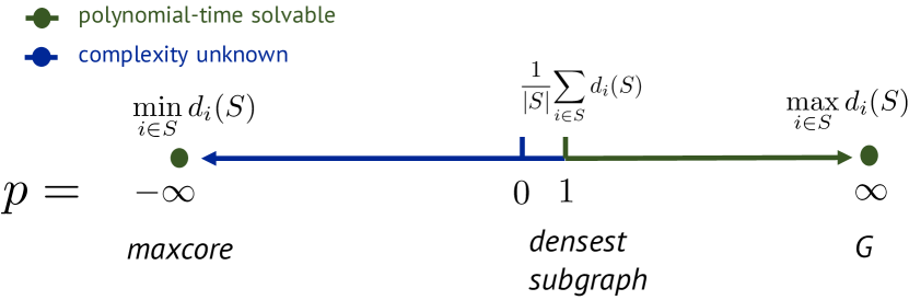
In light of these challenges, we define a simple, single-parameter family of objective functions for dense subgraph discovery. Our framework lets us (i) evaluate the tradeoffs between existing methods and (ii) uncover a hierarchy of dense subgraphs in the same graph, specifically in terms of the degree distribution of nodes in an induced subgraph. The family of objectives is motivated by a simple observation: the maxcore of a graph is the subgraph of maximum smallest induced degree, while the standard densest subgraph is the one of maximum average induced degree. Given that both of these are well-known and oft-used, it is natural to ask what other functions of induced node degrees are meaningful to optimize.
To answer this, we introduce the generalized mean densest subgraph problem, which is parameterized by a single parameter . We show that the maxcore and standard densest subgraph problems are obtained as special cases when and , respectively. Another existing notion of dense subgraphs that places a higher emphasis on large degrees is recovered when (Faragó, 2008). And the limiting case of is solved by simply returning the entire graph. Other values of lead to objectives that have not been considered previously, but correspond to natural alternative objectives for dense subgraph discovery. For example, in the case of , our problem is equivalent to finding a subgraph that maximizes the average logarithm of degree. Figure 1 summarizes the objective function landscape captured by our framework.
In addition to unifying a number of previous approaches, our framework is accompanied by several novel theoretical guarantees and algorithmic techniques for finding dense subgraphs. We first prove that our objective is polynomial-time solvable when , giving an algorithm based on repeated submodular minimization. We then present a variety of theoretical and empirical results on peeling algorithms for dense subgraph discovery in the context of our objective. These algorithms are approximation algorithms but are much faster than submodular minimization. They rely on repeatedly removing a single vertex at a time in order to shrink a graph down into a denser subgraph. The standard approach for peeling iteratively removes the node of smallest degree (Asahiro et al., 2000). Surprisingly, we prove that despite seeming like a natural approach, this well-known standard peeling algorithm, which optimally solves the objective (Matula and Beck, 1983) and provides a -approximation for the objective (Charikar, 2000; Khuller and Saha, 2009), can yield arbitrarily bad results when . However, we then design a more sophisticated but still fast peeling algorithm that is guaranteed to return a approximation for any . Although we prove that this bound is asymptotically tight, this approximation guarantee is always at least , and converges to as . When , both the method and its guarantee reduce to that of the standard peeling algorithm.
In order to greedily optimize the version of our objective, our method must take into account not only how removing a node affects its own degree (i.e., it disappears), but also how this affects the node’s neighbors in the graph and their contribution to the generalized objective. This gives our method a certain level of “foresight” when removing nodes, that is not present in the strategy of the standard peeling algorithm. In light of this observation, our framework contains both theoretical and empirical examples where our new peeling method can outperform the standard peeling algorithm in finding dense subgraphs. For example, on many real-world graphs, we find that running our method with a value of slightly larger than 1 will typically produce sets with a better average degree than standard peeling, even though our method is technically greedily optimizing a different objective.
We apply our methods on a range of different sized graphs from various domains, including social networks, road networks, citation networks, and web networks. We show that for small graphs with up to 1000 nodes, we can optimally find -mean densest subgraphs using submodular minimization, and that on these graphs our approximation algorithm does a much better job approximating the optimal sets than its theory guarantees. Our greedy peeling algorithm is also fast and scales to large datasets, and is able to uncover different meaningful notions of dense subgraphs in practice as we change our parameter .
In summary, we present the following contributions.
-
•
We introduce the generalized mean densest subgraph problem and show that the well-studied maxcore and densest subgraph problems are special cases.
-
•
We give a polynomial-time algorithm for optimally solving the objective for any , by showing that the decision version of the problem can be solved via submodular minimization. Existing linear-time algorithms solve the case, which reduces to maxcore.
-
•
We provide a faster greedy approximation algorithm that returns a approximation for . We show a class of graphs for which this approximation is tight. As , this approximation converges to 1. We also prove that for any , the greedy algorithm for the standard densest subgraph problem returns arbitrarily bad approximations on certain graph classes.
-
•
We use our framework and methods to identify a range of different types of dense subgraphs and compare the performance of different peeling algorithms, on graphs coming from a wide variety of domains.
2. Technical Preliminaries
Let be an undirected and unweighted graph. For , let denote the neighborhood of node , and be its degree. For a set , let denote the set of edges joining nodes in and be the degree of in the subgraph induced by . If , then .
Dense Subgraph Problems
The densest subgraph problem seeks a set of nodes that maximizes the ratio between the number of edges and nodes in the subgraph induced by :
| (1) |
The numerator of this objective is equal to half the sum of induced node degrees in , and therefore this problem is equivalent to finding the maximum average degree subgraph:
| (2) |
This problem is known to have a polynomial-time solution (Goldberg, 1984; Gallo et al., 1989), as well as a fast greedy peeling algorithm that is guaranteed to return a -approximation (Khuller and Saha, 2009; Charikar, 2000).
Another well-studied dense subgraph problem is to find the -core of a graph for a positive integer (Dorogovtsev et al., 2006; Carmi et al., 2007; Shin et al., 2016; Malliaros et al., 2020). The -core of a graph is a maximal connected subgraph in which all nodes have degree at least . The maximum value of for which the -core of a graph is non-empty is called the degeneracy of the graph. If is the degeneracy of , we will refer to the -core of as the maxcore. Finding the maxcore is equivalent to finding the subset that maximizes the minimum induced degree:
| (3) |
For any value of , the -core of a graph can be found in linear time via a greedy peeling algorithm that repeatedly removes nodes with degree less than (Matula and Beck, 1983).
Generalized Means
For a vector of positive real numbers , the generalized mean (power mean or -mean) with exponent of x is defined to be
| (4) |
For , the mean can be defined by taking limits, so that , , and (the case is often called the geometric mean).
Submodularity and the power function
We review a few useful preliminaries on submodular functions and properties of the power function for that will be useful for our algorithmic results. For a discrete set , a function is submodular if for any subsets it satisfies
| (5) |
If the above inequality is reversed, is referred to as a supermodular function, and if we replace it with equality, the function is called modular. We have the following two simple observations about properties of the power function, which follow from the fact that is concave when , and convex when .
Observation 1.
The function for is submodular when and supermodular when .
Observation 2.
Let and . Then
3. The -Mean Densest Subgraph
We now introduce a new single-parameter family of dense subgraph objectives based on generalized means of degree sequences. Abusing notation slightly, we define the -density of to be
| (6) |
The generalized mean densest subgraph problem is then to find a set of node that maximizes . We also refer to this as the -mean densest subgraph problem to make the parameter explicit. It is worthwhile to note that this objective increases monotonically with , ranging from the minimum degree of when to the maximum degree of when .
3.1. Equivalence Results and Special Cases
The definition of generalized mean, and the characterizations of the densest subgraph and max-core problem given in (2) and (3), immediately imply the following equivalence results.
Lemma 3.1.
The standard densest subgraph problem (2) is equivalent to the -mean densest subgraph problem. The maxcore objective is equivalent to the -mean densest subgraph problem.
Although studied less extensively, an equivalent variant of the -mean densest subgraph has also been previously considered (Faragó, 2008) as a way to find dense subgraphs that place a higher emphasis on the largest degrees. Our new objective therefore unifies existing dense subgraph problems, and suggests a natural way to interpolate them as well as find new meaningful notions of dense subgraphs.
For finite , maximizing is equivalent to maximizing . In other words, the -mean densest subgraph problem seeks a subgraph with the highest average th-power degree:
| (7) |
For , objective (7) is no longer meaningful, but from the standard definition of -mean we know that is simply the maximum degree of the induced subgraph. This makes intuitive sense given that objective (7) places higher and higher emphasis on large degrees as . The objective is trivially solved by taking the entire graph , though this will not necessarily be optimal for large but finite values of .
When , the generalized mean coincides with the geometric mean, which for our dense subgraph framework means that
| (8) |
As long as does not include zero degree nodes, maximizing this quantity is equivalent to maximizing , which amounts to finding the subgraph with maximum average log-degree:
| (9) |
While natural, this objective has not been previously considered for dense subgraph problems.
Finally, for finite , maximizing is equivalent to maximizing , which equals
| (10) |
In other words, while the objective maximizes the average degree, the objective seeks the to maximize one over the average inverse degree (corresponding to the harmonic mean of the degrees). For other the goal is to maximize one over the average th power of the degrees.
3.2. Comparison with Existing Objectives
Before moving on we compare and contrast our -mean objective against similar generalizations of the densest subgraph problem. See Section 6 for more related work.
The -clique densest subgraph. Tsourakakis (Tsourakakis, 2015) previously introduced the -clique densest subgraph problem (-DS), which seeks a set of nodes that minimizes the ratio between the number of -cliques and the number of nodes in . The standard densest subgraph problem is recovered when . The author showed that this objective can be maximized in polynomial time for any fixed value of , and also gave a -approximate peeling algorithm by generalizing the standard greedy peeling algorithm (Charikar, 2000; Asahiro et al., 2000). In practice, even when , maximizing this objective can produce subgraphs that are much closer to being near cliques than the standard densest subgraph solution.
F-density. An even more general objective called F-density was introduced by Faragó (Faragó, 2008). Given a family of graphs F, this objective seeks a set that maximizes the ratio between the number of instances of F-graphs in , and . The -DS problem is recovered when F includes only the clique on nodes. Interestingly, Faragó (Faragó, 2008) showed that when , where is the path graph on nodes, then the F-density is the following ratio:
| (11) |
The maximizers of this objective are the same as those for the -mean densest subgraph problem in our framework, although there are differences in terms of approximation guarantees of algorithms.
Discounted average degree and f-densest subgraph. The above objectives generalize the standard densest subgraph problem by changing the numerator of the objective. Generalizing in a different direction, Kawase and Miyauchi (Kawase and Miyauchi, 2018) introduced the -densest subgraph problem, which seeks a set maximizing for a convex or concave function . This includes the special case for , which generalizes the earlier notion of discounted average degree considered by Yanagisawa and Hara (Yanagisawa and Hara, 2018). When is concave, maximizing the objective will always produce output sets that are larger than or equal to optimizers for the densest subgraph problem. Convex produces outputs sets that are always smaller than or equal to densest subgraph solutions (Kawase and Miyauchi, 2018).
Comparison with -mean densest subgraph. The -mean densest subgraph problem is similar to the above objectives in that they are all parameterized generalizations of the densest subgraph problem. However, each generalizes the objective in a different direction. The -clique densest subgraph problem parameterizes preferences for obtaining clique-like subgraphs, while F-density more generally controls the search for dense subgraphs that are rich in terms of specified subgraph patterns (graphlets). The discounted average degree and -densest subgraph objectives reward set sizes differently, while keeping the same emphasis on counting edges in the induced subgraph. Meanwhile, our objective encapsulates different preferences in terms of induced node degrees. Many subcases amount to maximizing averages of different functions on node degrees. Importantly, the max-core problem is not captured as a special case of F-density, -DS, or the -densest subgraph.
Our objective and the -densest subgraph problem are tangentially similar in that they both can involve the power function in some way. However, a major difference is that the latter objective shares the same numerator (the induced edge count ) as the standard densest subgraph, which is not the case for our problem. This leads to substantial differences in terms of the computational complexity and the output sets that maximize these objectives. For example, the -densest subgraph with is NP-hard when and is guaranteed produce smaller output sets than the standard densest subgraph in this case, and is also known to have trivial constant-sized optimal solutions when (Kawase and Miyauchi, 2018). In contrast, is in fact the easier regime for our problem and will often, but not always, produce larger output sets. Finally, we note that the relationship between F-density and -mean density does not appear to generalize to other values of , even if we restrict to positive integer values of . In particular, by checking a few small examples, it is easy to confirm that the -mean density objective is not equivalent to F-density when .
4. Algorithms
We now present new algorithms for the -mean densest subgraph problem. We show that the objective can be solved in polynomial time for any via submodular minimization. For the same parameter regime, we show that the standard greedy peeling algorithm (Asahiro et al., 2000; Charikar, 2000; Khuller and Saha, 2009) can return arbitrarily bad results, but a more sophisticated generalization yields a approximation, which is also tight. Algorithms for appear more challenging—both our submodular minimization technique and greedy approximation do not hold in this case. Improved algorithms or hardness results for this regime are a compelling avenue for future research.
4.1. An Optimal Algorithm for
For finite , , so for simplicity we focus on the latter objective. In the next section we will use the fact that a -approximate solution for provides a approximate solution for .
Given a fixed , the decision version of our problem asks whether there exists some such that , or equivalently . We can obtain a yes or no answer to this question by solving the following optimization problem
When , it is well known that this can be solved by solving a minimum - cut problem (Goldberg, 1984), which is itself a special case of submodular minimization (equivalently, supermodular function maximization). The following result guarantees that we can still get a polynomial time algorithm for the -mean densest subgraph when by using general submodular minimization.
Lemma 4.1.
If and , the function is supermodular.
Proof.
The function is modular, so it suffices to show that the function is supermodular whenever . For a node and an arbitrary set , if then define . This allows us to write as a summation over all nodes in without loss of generality:
We would like to show that for arbitrary sets and , we have
which is true if we can show that for every and ,
| (12) |
To prove (12), let be the set of edges adjacent to , and note that all of the terms in inequality (12) represent the number of edges in a certain subset of . Specifically, define
Consider the sets obtained by unions and intersections of and :
These sets are related to sets of edges that contribute to degree counts for node :
Recall from Observation 1 that if is a discrete set, then the function for is supermodular whenever . Therefore, for these sets of edges,
So the desired inequality is shown. ∎
Using submodular minimization algorithms as a black box (Orlin, 2009), we can perform binary search on to find the maximum value of such that , which is equivalent to saying . The number of binary search steps necessary to exactly optimize can be easily bounded by a polynomial in . The number of different values that the numerator can take on is trivially bounded above by , as this is the number of distinct ways to bipartition the graph. The denominator can take on values. We can use and as bounds for our binary search, and even for an extremely pessimistic case, binary search steps would be necessary, though typically it will be far less in practice. We conclude the following result.
Theorem 4.2.
For any graph and , the -mean densest subgraph can be found in polynomial time.
This result is intended to serve mainly as a theoretical result confirming the polynomial-time solvability of the problem for . We next turn to more practical greedy approximation algorithms.
4.2. Failure of the Standard Peeling Algorithm
The standard peeling algorithm for both the maxcore and densest subgraph problem is to start with the entire graph and repeatedly remove the minimum degree node until no more nodes remain. We will refer to this algorithm generically as SimplePeel. This algorithm produces a set of subgraphs , one of which is guaranteed to solve the maxcore problem (Matula and Beck, 1983), and another of which is guaranteed to provide at least a -approximation to the standard densest subgraph problem (Charikar, 2000). Trivially, this method also yields and optimal solution for , since the entire graph solves the -mean objective.
Given the success of this procedure for , it is natural to wonder whether it can be used to obtain optimal or near optimal solutions for other values of . Focusing on the case, we know that if for a subset , then it is also true that , again suggesting that this strategy might be effective. However, surprisingly, we are able to show that the simple peeling algorithm can perform arbitrarily poorly for any . To show this, we consider the performance of the algorithm on the same class of graphs that has been used to show that the -approximation for the standard peeling algorithm is tight for the 1-mean objective (Khuller and Saha, 2009).
Lemma 4.3.
Let and be fixed constants. There exists a graph such that applying SimplePeel on will yield an approximation worse than for the th power degree objective.
Proof.
The proof is by construction. Let be a complete bipartite graph with nodes on one side and nodes on the other, and be a disjoint union of cliques of size . We treat as a fixed constant and as a value that will grow without bound. Define graph to be the union of and . We have , and
As , is the best -mean densest subgraph, with behaving as . However, SimplePeel will start by removing all of the nodes in , since on one side of the bipartite graph, all nodes have degree , whereas all nodes have degree . At the outset of the algorithm, we start with all of and note that
We see that as , this provides only a approximation to . As SimplePeel removes nodes from , the approximation gets worse, until we are left with a subgraph with maximum average th power degree of . Since was an arbitrary constant, we can choose . Then, for large enough we will have
Therefore, the approximation is worse than . ∎
The above result means that for any and fixed, there exists a graph with an optimal -mean densest subgraph , such that the simple greedy method will return a set satisfying
Since is fixed and is arbitrarily small, this means the simple greedy method can do arbitrarily badly when trying to approximate the -mean densest subgraph problem.
4.3. Generalized Peeling Algorithm when
The failure of SimplePeel can be explained by noting that when , removing a minimum degree node from a subgraph does not in fact greedily improve -density. Consider a node set and its average th power degree function . Removing any will change the denominator of in exactly the same way. Therefore, to greedily improve the objective by removing a single node, we should choose the node that leads to the minimum decrease in the numerator . Importantly, it is not necessarily the case that is the best node to remove. This would account only for the fact that the numerator decreases by , but ignores the fact that removing will also affect the degree of all other nodes that neighbor in . For example, if has a small degree but neighbors a high degree node , then when , removing node and decreasing ’s degree could substantially impact the -density objective. For a graph , node set , and arbitrary node , the following function reports the exact decrease in the numerator of resulting from removing :
| (13) |
In other words, note that is the numerator before removing , and after removing it we have a new numerator
Observe that when , , which explains why it suffices to remove the minimum degree node in order to greedily optimize the variant of the objective. Based on these observations, we define a generalized peeling algorithm, which we call GenPeel-, or simply GenPeel when is clear from context, based on iteratively removing nodes that minimize (13). Pseudocode is given in Algorithm 1. We prove the following result.
Theorem 4.4.
Let be a graph, , and be the -mean densest subgraph of . Then GenPeel- returns a subgraph satisfying , i.e., .
Proof.
Define , which implies that . Since is optimal, removing a node will produce a set with -density at most , and therefore, we have
Observe that for any set and we have . This holds because is larger than when we grow the subgraph, and also because the function also monotonically grows as gets bigger, as long as .
Let denote the set maintained by the greedy algorithm right before the first node is removed by peeling. Since is the first node to be removed by the peeling algorithm, we know that and . Because , we know is smaller than the average value of across nodes in , so
The last step follows from the bound in Observation 2. For every , the value show up exactly times in the double summation in the second term—once for every such that neighbors in . Therefore:
∎
In the appendix, we provide an in-depth graph construction to show that this approximation guarantee is asymptotically tight for all values of . Nevertheless, for , the quantity decreases monotonically and has a limit of one, meaning that the -density problem in fact becomes easier to approximate as we increase . In fact, the -approximation for the standard densest subgraph problem is the worst approximation that this method obtains for any . The fact that the approximation factor converges to 1 also intuitively matches the fact that when , the optimal solution is trivial to obtain by keeping all of .
Key differences between peeling algorithms. Before moving on, it is worth noting two key differences about removing nodes based on degree (SimplePeel) and removing nodes based on (GenPeel). The first is purely practical: it is faster to keep track of node degrees than to keep track of changes to for each node when peeling. Removing a node will change the degrees of nodes within a one-hop neighborhood, but will change values for every node within a two-hop neighborhood of . This additional detail complicates the runtime analysis and implementation of GenPeel. For , a naive runtime bound of can still be obtained by first realizing that as long as degrees are known, the value of can be computed in time, and so all values can be computed in time. There are rounds overall, and in each round it takes time to find the minimizer of , plus time to update degrees after a node is removed, plus time to update values in preparation for the next round.
Although this runtime bound is much worse than the linear time guarantee for the best implementation of SimplePeel, it is quite pessimistic, and in practice we can still scale up GenPeel to large datasets in practice. Furthermore, although GenPeel is slower, this difference in strategy is not without its advantages. The -approximation for SimplePeel is tight on certain graph classes made up of disjoint cliques and complete bipartite graphs (Khuller and Saha, 2009). This is also the same class of graphs we used to show that the method does arbitrarily badly when . SimplePeel fails to find the best subgraph on these instances because it considers the degree of a node without sufficiently considering the effect on its neighborhood. Meanwhile, GenPeel finds the optimal solution on these graph classes for all . In our next section, we will demonstrate empirically that running GenPeel with actually outperforms SimplePeel in optimizing the objective.
5. Experiments
We now consider how our methods enable us to find a range of different meaningful notions of dense subgraphs in practice. We begin by showing that GenPeel does an excellent job of approximating the optimal -mean densest subgraph problem, scales to large datasets, and detects subgraphs with a range of different meaningful notions of density. Using GenPeel- with can even be used to solve the objective (standard densest subgraph) better than SimplePeel (which is equivalent to GenPeel-) in many cases, even though SimplePeel greedily optimizes the objective but GenPeel- with does not. All of our experiments were performed on a laptop with 8GB of RAM and 2.2 GHz Intel Core i7 processor. We use public datasets from the SNAP repository (Leskovec and Krevl, 2014) and the SuiteSparse Matrix collection (Davis and Hu, 2011). We implement GenPeel and SimplePeel in Julia, both using a simple min-heap data structure for removing nodes, which works well in practice. We implement our optimal submodular minimization approach in MATLAB, in order to use existing submodular optimization software (Krause, 2010). All algorithm implementations and code for our experiments are available at https://github.com/nveldt/GenMeanDSG.
5.1. GenPeel Approximation Performance
| Astro | CM05 | BrKite | Enron | roadCA | roadTX | webG | webBS | Amaz | YTube | ||
| 17,903 | 36,458 | 58,228 | 36,692 | 1,971,281 | 1,393,383 | 916,428 | 685,230 | 334,863 | 1,134,890 | ||
| Metric | 196,972 | 171,734 | 21,4078 | 183,831 | 2,766,607 | 1,921,660 | 4,322,051 | 6,649,470 | 925,872 | 2,987,624 | |
| Size | maxcore | 57 | 30 | 154 | 275 | 4568 | 1579 | 48 | 392 | 497 | 845 |
| 165 | 30 | 200 | 469 | 4568 | 1579 | 229 | 392 | 497 | 1616 | ||
| 1151 | 563 | 219 | 548 | 11 | 3721 | 240 | 392 | 34 | 1863 | ||
| 1317 | 565 | 220 | 556 | 6 | 26 | 240 | 392 | 3848 | 1900 | ||
| 1564 | 742 | 242 | 713 | 12 | 91 | 243 | 5352 | 118 | 3085 | ||
| 1491 | 938 | 273 | 1036 | 185 | 13 | 4429 | 34944 | 550 | 29639 | ||
| Edge | maxcore | 1.0 | 1.0 | 0.502 | 0.256 | 0.001 | 0.002 | 0.994 | 0.529 | 0.014 | 0.102 |
| Density | 0.348 | 1.0 | 0.407 | 0.159 | 0.001 | 0.002 | 0.235 | 0.529 | 0.014 | 0.056 | |
| 0.052 | 0.056 | 0.372 | 0.137 | 0.345 | 0.001 | 0.227 | 0.529 | 0.23 | 0.049 | ||
| 0.045 | 0.056 | 0.37 | 0.135 | 0.733 | 0.166 | 0.227 | 0.529 | 0.002 | 0.048 | ||
| 0.039 | 0.043 | 0.335 | 0.104 | 0.333 | 0.044 | 0.225 | 0.031 | 0.082 | 0.029 | ||
| 0.041 | 0.032 | 0.29 | 0.068 | 0.02 | 0.295 | 0.005 | 0.001 | 0.005 | 0.001 | ||
| Avg | maxcore | 56.0 | 29.0 | 76.87 | 70.06 | 3.32 | 3.34 | 46.71 | 206.81 | 6.77 | 86.07 |
| Degree | 57.02 | 29.0 | 80.91 | 74.38 | 3.32 | 3.34 | 53.58 | 206.81 | 6.77 | 90.76 | |
| 59.28 | 31.57 | 81.11 | 74.68 | 3.45 | 3.49 | 54.36 | 206.81 | 7.59 | 91.16 | ||
| 59.25 | 31.58 | 81.12 | 74.69 | 3.67 | 4.15 | 54.36 | 206.81 | 8.7 | 91.18 | ||
| 60.74 | 31.61 | 80.8 | 73.96 | 3.67 | 4.0 | 54.47 | 166.93 | 9.56 | 88.86 | ||
| 60.92 | 30.32 | 78.99 | 70.35 | 3.62 | 3.54 | 20.39 | 44.04 | 2.65 | 19.88 | ||
| Avg | maxcore | 3136.0 | 841.0 | 6335.5 | 5685.5 | 11.3 | 11.7 | 2182.4 | 43840.3 | 47.4 | 9227.8 |
| Squared | 3297.6 | 841.0 | 7372.9 | 7002.2 | 11.3 | 11.7 | 2930.9 | 43840.3 | 47.4 | 11486.8 | |
| Degree | 4154.3 | 1265.8 | 7614.1 | 7301.6 | 12.2 | 12.7 | 3031.9 | 43840.3 | 59.2 | 12146.5 | |
| 4226.3 | 1269.0 | 7624.9 | 7336.1 | 13.7 | 19.2 | 3031.9 | 43840.3 | 189.3 | 12220.1 | ||
| 4691.7 | 1356.1 | 7776.6 | 7691.7 | 13.7 | 17.3 | 3051.2 | 157225.3 | 372.9 | 14359.8 | ||
| 5106.6 | 1384.1 | 7882.1 | 7918.9 | 13.9 | 18.6 | 9730.9 | 455975.9 | 552.3 | 33262.3 | ||
| Max | maxcore | 56 | 29 | 153 | 216 | 7 | 12 | 47 | 391 | 13 | 447 |
| Degree | 108 | 29 | 196 | 302 | 7 | 12 | 82 | 391 | 13 | 844 | |
| 241 | 161 | 214 | 333 | 4 | 12 | 84 | 391 | 10 | 954 | ||
| 281 | 163 | 215 | 338 | 4 | 8 | 84 | 391 | 161 | 978 | ||
| 333 | 200 | 233 | 399 | 4 | 8 | 86 | 5351 | 106 | 1428 | ||
| 392 | 257 | 260 | 513 | 9 | 12 | 2329 | 34943 | 549 | 28754 | ||
| Runtime | maxcore | 0.03 | 0.03 | 0.06 | 0.04 | 1.37 | 0.96 | 2.4 | 11.27 | 0.45 | 2.51 |
| 0.29 | 0.19 | 0.38 | 0.46 | 4.8 | 3.41 | 51.28 | 608.5 | 2.01 | 58.87 | ||
| 0.03 | 0.03 | 0.06 | 0.04 | 1.37 | 0.96 | 2.4 | 11.27 | 0.45 | 2.51 | ||
| 0.25 | 0.18 | 0.35 | 0.4 | 4.4 | 3.0 | 41.92 | 490.91 | 1.62 | 39.21 | ||
| 0.26 | 0.17 | 0.32 | 0.37 | 4.29 | 3.14 | 39.64 | 324.67 | 1.67 | 30.26 | ||
| 0.25 | 0.17 | 0.32 | 0.35 | 4.12 | 3.07 | 19.13 | 295.73 | 1.69 | 26.17 |
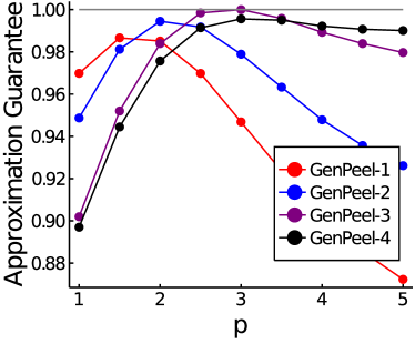
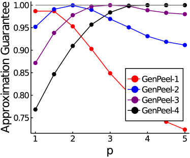
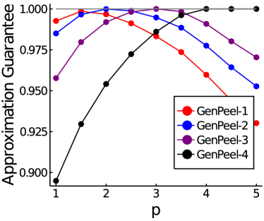
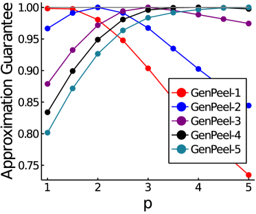
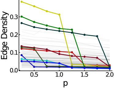
In practice, GenPeel can find a dense subgraph that approximates the optimal solution much better than its worst case guarantee. Furthermore, both the optimal -mean densest subgraphs for different , and the sets found by GenPeel using different , are meaningfully distinct from each other and highlight different notions of density in real-world graphs. To demonstrate this, we find a set of optimal solutions to our objective for values in . We solve our objective exactly on graphs with up to 1000 nodes to within a small tolerance with a MATLAB implementation that uses existing submodular minimization software as a black box (Krause, 2010). We then run GenPeel for each . This produces 5 dense subgraphs, and we evaluate how each one approximates the optimal solution for all .
As expected, GenPeel- provides the best approximation for all near . Rounded curves in Figure 2 show that each run of GenPeel optimizes a different regime of our problem. For three datasets, the solutions are identical, both at optimality and for the sets returned by GenPeel. Otherwise, we see a clear distinction between the output curves for each run of the algorithm, indicating that we are finding different types of dense subgraphs.
5.2. Peeling Algorithms for Dense Subgraphs
Out next set of experiments places the standard greedy peeling algorithm for densest subgraph () and the peeling algorithm for finding maxcore () within a broader context of parametric peeling algorithms for dense subgraph discovery. By comparing these outputs against GenPeel for different values near 1, we can observe how each method emphasizes and favors different notions of density in the graph. We can also see how running GenPeel for values near but not equal to one provides an accuracy vs. runtime tradeoff when it comes to finding sets that satisfy the traditional notion of density.
We run GenPeel for . Although our method provides no formal guarantees when , it nevertheless greedily optimizes the -mean density objective and produces meaningfully different subgraphs. When , our implementation defaults to running the faster SimplePeel algorithm, and also outputs the maxcore solution, as this is obtained by simple peeling with a different stopping point. We focus on the regime in order to better understand how different desirable measures of density vary as we explore above and below the standard densest subgraph regime (). Additionally, restricting to means we are interpolating between objectives that have previously been studied (Matula and Beck, 1983; Charikar, 2000; Faragó, 2008), and avoids placing too high of an emphasis on just finding a small number of very high degree nodes.
Table 1 displays runtimes and subgraph statistics for each peeling result on a range of familiar benchmark graphs from a variety of different domains. This includes two citation networks (ca-Astro, condmat2005), two road networks (road-CA, road-TX), two web graphs (web-Google, web-BerkStan), an email network (Enron), two social networks (BrightKite, YouTube), and a retail graph (Amazon). We report the edge density (number of edges divided by number of pairs of nodes), the size of the set returned, and the average degree (i.e., the objective). There are clear trends in the output of each method: as decreases, the subgraphs tend to be smaller and have a higher edge density. As increases from 0.5 to 2, the average squared degree and the maximum degree increase significantly. What is perhaps most significant is that running GenPeel- with tends to produce better sets than SimplePeel in terms of the standard densest subgraph objective. We conjecture that this is because GenPeel makes more strategic node removal decisions based not only on a node’s degree, but also on the degree of its neighbor. This comes at the expense of a slower runtime, but we still find that our method is fast and scales up to very large graphs.
5.3. Dense Subgraphs in Social Networks
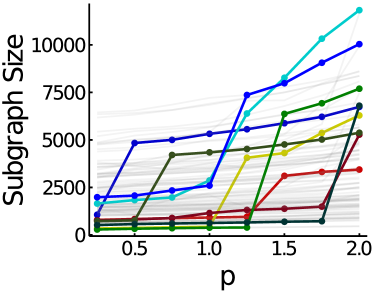
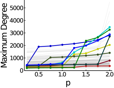
Finally, we use GenPeel to detect different types of dense subgraphs in social networks. We run our method for , on all graphs from the Facebook100 dataset (Traud et al., 2012). Each graph is a snapshot of the Facebook network at a US university. The graphs have 700–42k nodes. For each of the 100 graphs, we plot curves indicating how the average degree, size, maximum degree, and edge density changes as increases (Figure 4). In this parameter regime, the average degree of subgraphs returned hardly varies (Figure 4a). Increasing tends to produce subgraphs that are larger and have a higher maximum degree (Figures 4b and 4c), while decreasing produces smaller sets with higher edge density (Figure 4d). We again find that running GenPeel with can often find sets with higher average degree. This happens on six Facebook graphs when (Figure 4a). We separately ran GenPeel with on all graphs, and found that it returned sets with higher average degree than SimplePeel on 42 out of the 100 graphs.
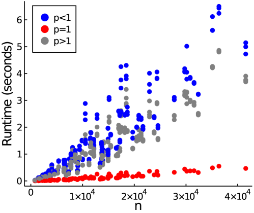
Figure 3 is a scatter plot of points (,) where is the number of nodes in a Facebook graph and the the time in seconds for our algorithm. When , the method is much faster as it only considers node degree when greedily removing nodes. For the case, runtime are still very fast and still scale roughly linearly, though with a steeper slope. For and , the same exact procedure is applied. The case nevertheless tends to take slightly longer, perhaps simply because greedy node removal in this regime can lead to more drastic changes in the function that the algorithm must update at each iteration. Still, on even the largest graphs, GenPeel takes just a few seconds.

6. Related Work
In order to situate our research within a broader context, we briefly review other related work on dense subgraph discovery. The standard densest subgraph problem is known to be polynomial time solvable via reduction to a maximum - flow problem (Gallo et al., 1989; Goldberg, 1984). When the goal is to find the densest subgraph on nodes, the problem becomes NP-hard (Feige et al., 2001). A number of methods for finding dense subgraphs focus specifically on greedy peeling algorithms. The standard peeling algorithm for dense subgraph discovery was first proposed by Ashahiro et al. (Asahiro et al., 2000) as a means to approximate the latter task, but was later shown by Charikar (Charikar, 2000) to provide a -approximation to the unrestricted objective. This approximation was later adapted by Khuller and Saha (Khuller and Saha, 2009) to provide an approximation in the case of directed graphs, a variant that can also be solved in polynomial time. A number of generalizations of the objective have recently been considered, including the -clique densest subgraph (Tsourakakis, 2015), the F-density objective (Faragó, 2008), the -densest subgraph (Kawase and Miyauchi, 2018), and generalizations involving signed graphs (Tsourakakis et al., 2019), bipartite graphs (Sarıyüce and Pinar, 2018), and fairness constraints (Anagnostopoulos et al., 2020). Outside of direct variations on the densest subgraph problem that we generalized, other formalisms for similar dense subgraphs include nucleus decompositions (Sariyuce et al., 2015), quasi-cliques (Tsourakakis et al., 2013), trusses (Cohen, 2008), braces (Ugander et al., 2012), DN-graphs (Wang et al., 2010), plexes (Seidman and Foster, 1978), and clubs and clans (Mokken et al., 1979). For additional related work, we refer to the survey by Lee et al. (Lee et al., 2010) and a tutorial from Gionis and Tsourakakis (Gionis and Tsourakakis, 2015).
7. Conclusion and Discussion
Our -mean densest subgraph objective unifies the standard densest subgraph and maxcore problems, and provides a general framework for capturing different notions of density in the same graph. We have presented several new algorithmic guarantees, including an optimal polynomial time solution based on submodular minimization, and a fast approximation algorithm based on a more sophisticated variant of the standard peeling method. The most compelling direction for future work is to develop computational complexity results and algorithms for . Experimental results using the greedy approximation for indicate that this regime favors smaller clusters with a higher edge density, which is a particularly attractive property in dense subgraph discovery. A question that remains open even for is whether a single peeling algorithm or alternative ordering method on the nodes can be used to define a nested set of dense subgraphs that can well approximate our objective for a wide range of values, simply by adding or subtracting additional nodes from the ordering as changes. In many of our experiments, the greedy method return subgraphs that were often nested or at least nearly nested. This therefore seems like a promising avenue for future theoretical results, or at least new practical techniques that provide a range of dense subgraphs without re-running an algorithm for each value of .
Acknowledgements.
This research was supported by NSF Award DMS-1830274, ARO Award W911NF19-1-0057, ARO MURI, JPMorgan Chase & Co, a Vannevar Bush Faculty Fellowship, and a Simons Investigator grant.References
- (1)
- Anagnostopoulos et al. (2020) Aris Anagnostopoulos, Luca Becchetti, Adriano Fazzone, Cristina Menghini, and Chris Schwiegelshohn. 2020. Spectral Relaxations and Fair Densest Subgraphs. In CIKM.
- Andersen and Chellapilla (2009) Reid Andersen and Kumar Chellapilla. 2009. Finding dense subgraphs with size bounds. In WAW.
- Angel et al. (2012) Albert Angel, Nick Koudas, Nikos Sarkas, and Divesh Srivastava. 2012. Dense Subgraph Maintenance under Streaming Edge Weight Updates for Real-time Story Identification. VLDB (2012).
- Asahiro et al. (2000) Yuichi Asahiro, Kazuo Iwama, Hisao Tamaki, and Takeshi Tokuyama. 2000. Greedily Finding a Dense Subgraph. J Algorithm (2000).
- Carmi et al. (2007) Shai Carmi, Shlomo Havlin, Scott Kirkpatrick, Yuval Shavitt, and Eran Shir. 2007. A model of Internet topology using k-shell decomposition. PNAS U.S.A (2007).
- Charikar (2000) Moses Charikar. 2000. Greedy approximation algorithms for finding dense components in a graph. In APPROX.
- Cohen (2008) Jonathan Cohen. 2008. Trusses: Cohesive subgraphs for social network analysis. Technical Report. National Security Agency.
- Davis and Hu (2011) Timothy A. Davis and Yifan Hu. 2011. The University of Florida Sparse Matrix Collection. ACM Trans. Math. Softw. (2011).
- Dorogovtsev et al. (2006) Sergey N Dorogovtsev, Alexander V Goltsev, and Jose Ferreira F Mendes. 2006. K-core organization of complex networks. Phys. Rev. Lett (2006).
- Faragó (2008) András Faragó. 2008. A general tractable density concept for graphs. Mathematics in Computer Science 1, 4 (2008), 689–699.
- Feige et al. (2001) Uriel Feige, David Peleg, and Guy Kortsarz. 2001. The dense k-subgraph problem. Algorithmica 29, 3 (2001), 410–421.
- Fratkin et al. (2006) Eugene Fratkin, Brian T Naughton, Douglas L Brutlag, and Serafim Batzoglou. 2006. MotifCut: regulatory motifs finding with maximum density subgraphs. Bioinformatics 22, 14 (2006), e150–e157.
- Gallo et al. (1989) Giorgio Gallo, Michael D Grigoriadis, and Robert E Tarjan. 1989. A fast parametric maximum flow algorithm and applications. SIAM J. Comput. 18, 1 (1989), 30–55.
- Gionis and Tsourakakis (2015) Aristides Gionis and Charalampos E Tsourakakis. 2015. Dense subgraph discovery: KDD 2015 tutorial. In KDD.
- Goldberg (1984) Andrew V Goldberg. 1984. Finding a maximum density subgraph. Technical Report. University of California, Berkeley.
- Hu et al. (2005) Haiyan Hu, Xifeng Yan, Yu Huang, Jiawei Han, and Xianghong Jasmine Zhou. 2005. Mining coherent dense subgraphs across massive biological networks for functional discovery. Bioinformatics 21 (2005), i213–i221.
- Karp (1972) Richard M Karp. 1972. Reducibility among combinatorial problems. In Complexity of computer computations. Springer, 85–103.
- Kawase and Miyauchi (2018) Yasushi Kawase and Atsushi Miyauchi. 2018. The Densest Subgraph Problem with a Convex/Concave Size Function. Algorithmica (2018).
- Khuller and Saha (2009) Samir Khuller and Barna Saha. 2009. On finding dense subgraphs. In International Colloquium on Automata, Languages, and Programming. Springer, 597–608.
- Krause (2010) Andreas Krause. 2010. SFO: A Toolbox for Submodular Function Optimization. J. Mach. Learn. Res (2010).
- Lanciano et al. (2020) Tommaso Lanciano, Francesco Bonchi, and Aristides Gionis. 2020. Explainable Classification of Brain Networks via Contrast Subgraphs. In KDD.
- Lee et al. (2010) Victor E Lee, Ning Ruan, Ruoming Jin, and Charu Aggarwal. 2010. A survey of algorithms for dense subgraph discovery. In Managing and Mining Graph Data. Springer, 303–336.
- Leskovec and Krevl (2014) Jure Leskovec and Andrej Krevl. 2014. SNAP Datasets: Stanford Large Network Dataset Collection. http://snap.stanford.edu/data. (June 2014).
- Malliaros et al. (2020) Fragkiskos D Malliaros, Christos Giatsidis, Apostolos N Papadopoulos, and Michalis Vazirgiannis. 2020. The core decomposition of networks: Theory, algorithms and applications. VLDB (2020).
- Matula and Beck (1983) David W. Matula and Leland L. Beck. 1983. Smallest-Last Ordering and Clustering and Graph Coloring Algorithms. J. ACM (1983).
- Mokken et al. (1979) Robert J Mokken et al. 1979. Cliques, clubs and clans. Qual. Quant (1979).
- Orlin (2009) James B. Orlin. 2009. A faster strongly polynomial time algorithm for submodular function minimization. Math. Program (2009).
- Pattillo et al. (2013) Jeffrey Pattillo, Alexander Veremyev, Sergiy Butenko, and Vladimir Boginski. 2013. On the maximum quasi-clique problem. Discret. Appl. Math. (2013).
- Qin et al. (2015) Lu Qin, Rong-Hua Li, Lijun Chang, and Chengqi Zhang. 2015. Locally Densest Subgraph Discovery. In KDD.
- Sarıyüce and Pinar (2018) Ahmet Erdem Sarıyüce and Ali Pinar. 2018. Peeling Bipartite Networks for Dense Subgraph Discovery. In WSDM.
- Sariyüce et al. (2018) Ahmet Erdem Sariyüce, C. Seshadhri, and Ali Pinar. 2018. Local Algorithms for Hierarchical Dense Subgraph Discovery. VLDB (2018).
- Sariyuce et al. (2015) Ahmet Erdem Sariyuce, C Seshadhri, Ali Pinar, and Umit V Catalyurek. 2015. Finding the hierarchy of dense subgraphs using nucleus decompositions. In WWW.
- Seidman (1983) Stephen B. Seidman. 1983. Network structure and minimum degree. Social Networks 5, 3 (1983), 269–287.
- Seidman and Foster (1978) Stephen B Seidman and Brian L Foster. 1978. A graph-theoretic generalization of the clique concept. Journal of Mathematical sociology 6, 1 (1978), 139–154.
- Shin et al. (2016) Kijung Shin, Tina Eliassi-Rad, and Christos Faloutsos. 2016. Corescope: Graph mining using k-core analysis—patterns, anomalies and algorithms. In ICDM.
- Shin et al. (2018) Kijung Shin, Tina Eliassi-Rad, and Christos Faloutsos. 2018. Patterns and anomalies in k-cores of real-world graphs with applications. KAIS (2018).
- Sozio and Gionis (2010) Mauro Sozio and Aristides Gionis. 2010. The community-search problem and how to plan a successful cocktail party. In KDD.
- Traud et al. (2012) Amanda L. Traud, Peter J. Mucha, and Mason A. Porter. 2012. Social structure of Facebook networks. Physica A (2012).
- Tsourakakis (2015) Charalampos Tsourakakis. 2015. The k-clique densest subgraph problem. In WWW.
- Tsourakakis et al. (2013) Charalampos Tsourakakis, Francesco Bonchi, Aristides Gionis, Francesco Gullo, and Maria Tsiarli. 2013. Denser than the Densest Subgraph: Extracting Optimal Quasi-Cliques with Quality Guarantees. In KDD.
- Tsourakakis et al. (2019) Charalampos E Tsourakakis, Tianyi Chen, Naonori Kakimura, and Jakub Pachocki. 2019. Novel dense subgraph discovery primitives: Risk aversion and exclusion queries. In ECML PKDD.
- Ugander et al. (2012) Johan Ugander, Lars Backstrom, Cameron Marlow, and Jon Kleinberg. 2012. Structural diversity in social contagion. Proc. Natl. Acad. Sci. U.S.A (2012).
- Veldt et al. (2018) Nate Veldt, David F. Gleich, and Anthony Wirth. 2018. A Correlation Clustering Framework for Community Detection. In WWW.
- Wang et al. (2010) Nan Wang, Jingbo Zhang, Kian-Lee Tan, and Anthony KH Tung. 2010. On triangulation-based dense neighborhood graph discovery. VLDB (2010).
- Yanagisawa and Hara (2018) Hiroki Yanagisawa and Satoshi Hara. 2018. Discounted average degree density metric and new algorithms for the densest subgraph problem. Networks (2018).
- Zhang et al. (2017) Si Zhang, Dawei Zhou, Mehmet Yigit Yildirim, Scott Alcorn, Jingrui He, Hasan Davulcu, and Hanghang Tong. 2017. Hidden: hierarchical dense subgraph detection with application to financial fraud detection. In SDM.
Appendix A Tightness of -GenPeel
For a graph and a fixed , define
| (14) |
This is the minimum change to the average th power degree of , and mirrors our definition of in (13). In order to find examples where the approximation guarantee of GenPeel- is tight, we would like to find graphs and such that (i) the -mean densest subgraph of is all of for , (ii) , and (iii) .
If we can satisfy these three requirements, we can build a graph for which GenPeel- returns an approximation that asymptotically approaches . To construct such an example, combine a single copy of with a large number of disjoint copies of to form a new graph . The above properties guarantee that is the maximum -densest subgraph of , but the peeling algorithm will nevertheless remove all of its nodes before removing any node from any copy of . As long as there are enough copies of (which we can add to without limit), the maximum -density returned by GenPeel- will be roughly , for an overall approximation of .
Specific Graph Construction
Let be an integer we will choose later and be a clique on nodes. Note that
Next, let be a graph parameterized by integers and , where is the number of nodes in . For each node , introduce an edge from to , where . This means that most nodes will have degree , while nodes close to 1 and close to will have slightly smaller degree. Overall, as long as is large compared to , we will have . More precisely, we can calculate that
Importantly, is nearly the same as , and in fact converges to if is fixed and . In detail, note that the minimum degree node is node , and so
Next, we need to choose a value of so that the greedy algorithm will opt to remove nodes from before removing nodes from one of the copies of . This will happen as long as
Choosing , we have
By Observation 2, we know that , and so
To compute the asymptotic approximation guarantee for GenPeel-, note that and so
Therefore, for any fixed finite , if satisfies and , then this overall quantity converges to . This means that asymptotically, the average th power degree of is times better than the average th power degree of , so this is the best approximation guarantee we can obtain after has been deleted. The set with the best density considered by GenPeel- will be the entire graph , since the density will be slightly better before we delete . However, we still have the same asymptotic approximation guarantee, since we can include copies of when forming , making asymptotically close to . For small values of (e.g., integers up to 10), it is not hard to numerically find examples of graphs with approximation guarantees between and , using this type of graph construction.