Heat pulse propagation and nonlocal phonon heat transport in one-dimensional harmonic chains

Abstract

Phonons are the main heat carriers in semiconductor devices. In small devices, heat is not driven by a local temperature gradient, but by local points of heat input and removal. This complicates theoretical modeling. Study of the propagation of vibrational energy from an initial localized pulse provides insight into nonlocal phonon heat transport. We report simulations of pulse propagation in one dimension. The 1d case has tricky anomalies, but provides the simplest pictures of the evolution from initially ballistic toward longer time diffusive propagation. Our results show surprising details, such as diverse results from different definitions of atomistic local energy, and failure to exhibit pure diffusion at long times. Boltzmann phonon gas theory, including external energy insertion, is applied to this inherently time-dependent and nonlocal problem. The solution, using relaxation time approximation for impurity scattering, does not closely agree with the simulated results.

I Introduction

When heat is inserted in a local region of a semiconductor, phonons (labeled by $Q=(\vec{q},j)$, wavevector and branch) carry heat ballistically until they scatter. The mean free path $\ell_{Q}$ of different phonons is very diverse. At large distances from the source, the local heat current $j(r,t)$ is no longer ballistic. The propagation of current beomes increasingly diffusive. Modelling of the crossover from ballistic to diffusive is difficult. It can be illuminated by simulations of simple model cases. The one-dimensional chain is the simplest model, with only one branch of phonons. In spite of the worry of oversimplifying the problem, the clarity of one-dimensional pictures provides some useful insights.

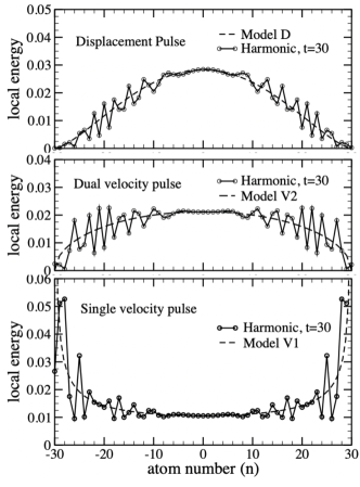
Figure 1: Circles connected by solid lines are the computed local energy $E_{a}(\ell)$ at $t=30$ for three types of pulses (see Eq. LABEL:eq:Eell and Table 1). All three pulses evolve from energy inserted at $t=0$ and $r\sim 0$ into a harmonic chain. The D and V2 pulses are initiated on atoms 0 and 1, but their positions on the horizontal axis are shifted by -1/2 to make them symmetric around $r=0$. The dashed curves are models derived from a continuum picture, such as Boltzmann theory, and given in Eqs. 10, 11, 12.

Figure 1 shows the local energy at atom sites on a one-dimensional chain of $N=200$ atoms coupled by nearest-neighbor harmonic springs. The system has periodic boundary conditions. At time $t=0^{-}$, the chain is in its ground state. At $t=0$, one or two central atoms are disturbed, starting a pulse. No further external disturbance is applied. The classical time evolution is computed from Newton’s laws. This is the simple example analyzed in this paper. In section II, the chain and the pulses are defined. In section III, the definition of “local energy” is analyzed and found to be more interesting than expected. In section IV, a continuum description is chosen and shown to explain the different results shown in Fig. 1. In section V, the Boltzmann equation is written for the nonlocal time-dependent problem, and its collisionless limit is shown to agree with the previously chosen continuum description. In section VI, simulations are repeated for an ensemble of mass-disordered chains, showing evolution in time in a direction toward diffusive energy propagation. In section VII, “pure” diffusion is defined, and shown to have imperfect ability to accurately explain heat propagation at long times. Section VIII returns to the Boltzmann description, with scattering from mass disorder added. The one-dimensional chain presents difficulties in the perturbative description of such scattering. The relaxation-time approximation (RTA) gives a sensible-looking approximate formula but is found not to agree accurately with the simulated energy propagation. Section IX gives a brief presentation of the effect of anharmonic scattering on the 1-d pulses. Section X summarizes the conclusions.

The main points of this paper are: (1) To clarify the ideas of local heat and local temperature. (2)To study the “crossover” from the ballistic propagation of Fig. 1 toward diffusive heat propagation when phonons start to evolve toward a local equilibrium $T(r,t)$ because of scattering Liu et al. (2014); Vermeersch et al. (2015). (3) To test the form and the accuracy of a non-local Boltzmann equation description Hua and Lindsay (2020).

II The harmonic linear chain

The chain has atoms of mass $M=1$ separated by distance $a=1$ and connected by springs of constant $K=1$. The harmonic normal modes have frequency $\omega_{Q}=\omega_{M}\sin(Qa/2)$ where $\omega_{M}=2\sqrt{K/M}=2$. Time is measured in units $\sqrt{M/K}=2/\omega_{M}=1$. The modes propagate at velocities $v_{Q}=v_{M}\cos(Qa/2){\rm sign}(Q)$ where $v_{M}=\sqrt{(}K/M)a=1$. The unit of energy is $E_{0}=1=Ka^{2}=Mv_{M}^{2}=M\omega_{M}^{2}a^{2}/4$. The leading edges of the pulse propagate at the speed of sound, $\pm v_{M}=\pm 1$, as is seen at $t=30$ in Fig. 1.

The Hamiltonian of the chain is

$$\mathcal{H}=\sum_{\ell}\left[\frac{P_{\ell}^{2}}{2M}+\frac{1}{2}K(u_{\ell}-u_{\ell+1})^{2}\right].$$ (1)

Atoms have displacements $u_{\ell}$ around average positions $r_{\ell}=\ell a$. The general solution of Newton’s equations of motion is

$$u_{\ell}(t)=\sqrt{\frac{1}{N}}\sum_{Q}A_{Q}\cos(Q\ell a-\omega_{Q}t+\phi_{Q}),$$ (2)

There are $2N$ free parameters, amplitude $A_{Q}\geq 0$ and phase $\phi_{Q}$ for each normal mode $Q$. The wavevector has the form $Q=(2\pi/a)(n/N)$, and the integer $n$ lies in the range $-N/2<n\leq N/2$. The pulses shown in Fig. 1, labeled D, V2, and V1, are generated by initial disturbances given in Table 1. The “V1” (or “velocity”) pulse has only the central atom given a velocity $v_{0}$ at $t=0$. The “V2” (or “dual velocity”) pulse has two central atoms given equal and opposite velocities. The “D” (or “displacement”) pulse has two central atoms given equal and opposite displacements at $t=0$.

The first result to notice is the interesting diversity of pulse shapes for different initial disturbances, as was first noticed in ref. Hua et al., 2017. The first issue to resolve is whether local energy is well-defined.

name	$\Delta u_{0}$	$\Delta u_{1}$	$\Delta v_{0}$	$\Delta v_{1}$
V1	0	0	$\sqrt{2}$	0
V2	0	0	-1	1
D	$-1/\sqrt{3}$	$1/\sqrt{3}$	0	0

Table 1: Properties of pulses. The shift $\Delta u$ (in units of $a$) of initial displacement, or $\Delta v$ (in units of $v_{M}$) of initial velocity, is scaled so that the new coordinates ($u_{0}+\Delta u_{0},\ u_{1}+\Delta u_{1},\ v_{0}+\Delta v_{0},\ v_{1}+\Delta v_{1}$), of atoms $\ell=0$ and $1$, have total extra energy $E_{\rm pulse}=1$. The values in the table give $E_{\rm pulse}=0$ at $T=0$, i.e. when $u_{\ell}(t)=0$ for $t<0$

III Defining local energy

Local energy $E(\ell,t)$ cannot be unambiguously defined Hardy (1963). In classical physics it should obey $\sum_{\ell}E(\ell,t)=\mathcal{H}$. The version plotted in Fig. 1 is defined as

$$E_{a}(\ell,t) = \frac{Mv_{\ell}(t)^{2}}{2}$$

$$+ \frac{K}{4}\left[(u_{\ell-1}(t)-u_{\ell}(t))^{2}+(u_{\ell}(t)-u_{\ell+1}(t))^{2}\right].$$

Each atom is assigned its own kinetic energy, and half of the potential energy of the springs to its left and right. This is a commonly used definition, but is not unique. Two other sensible choices for distributing potential energy to different sites are

$$E_{b}(\ell)=\frac{Mv_{\ell}^{2}}{2}+\frac{K}{2}\left[(2u_{\ell}^{2}-u_{\ell}(u_{\ell-1}+u_{\ell+1})\right],$$ (4)

$$E_{c}(\ell)=\frac{Mv_{\ell}^{2}}{2}\ {\rm and}\ E_{c}(\ell+1/2)=\frac{V}{2}(u_{\ell}-u_{\ell+1})^{2}.$$ (5)

The conventional version $E_{a}$ will be used in this paper, but it is interesting to see how it compares with versions $E_{b}$ and $E_{c}$, as shown in Fig. 2. The large oscillations seen in version (c) are surprising, and the smoothness seen in version (b) is even more surprising. This diversity illustrates our second result, a well-known fact: local energy at the atom level is not a clear concept. However, if local energy is averaged over a few nearby atoms, it becomes less diverse. The ambiguity also exists in quantum treatments. Marcolongo et al. Marcolongo et al. (2016) and Ercole et al. Ercole et al. (2016) have shown how this ambiguity does not affect the computation of bulk transport. In the next section we will see that local energy makes more sense in a continuum theory than an atomistic theory.

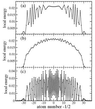
Figure 2: The harmonic V2 pulse at temperature $T=0$ and time $t=30$, using three ways (Eqs. LABEL:eq:Eell-5) of assigning potential energy to a local site energy, $E(\ell)$. In (a) and (b), the pulse energy is $E_{\rm pulse}=E_{0}=\sum_{\ell}E(\ell)$. The area under the curves is $E_{0}$, chosen to be 1. In (c), however, the energy has two parts, $\sum_{\ell}[KE(\ell)+PE(\ell+1/2)]$. The values in the graph have been arbitrarily doubled so that the total energy, also 1, is the area under the graph. These graphs demonstrate that the “continuum picture” of energy density (the dashed curves in Fig. 1) is more sensible than these local pictures.

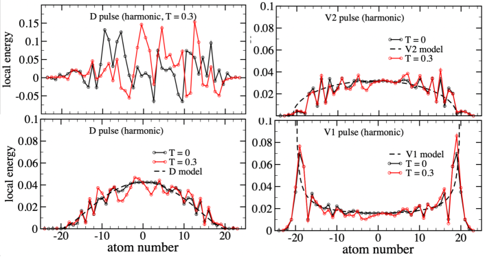
Figure 3: Pulses of total energy $\sum_{\ell}\Delta E_{a}(\ell)=E_{0}=1$ at $t=20$, inserted at $t=0$ to harmonic chains whose random positions and velocites at $t=0^{-}$ are thermalized at temperature $T=0.3$ ($E_{\rm tot,th}=0.3N$). The local energies $\Delta E_{a}(\ell)$ shown in the graphs are the differences between $E_{a}(\ell,t=20)$ with and without pulse insertion. The first graph shows D pulses inserted with two typical initial conditions. The other graphs show, in red, the results averaged over 1000-member ensembles with random thermal initial conditions. The black results repeat the zero-temperature pulses shown in Fig. 1. The finite $T$ pulse shapes, after ensemble averaging, are converging towards the zero-temperature pulse shapes.

Figure 1 shows $E_{a}(\ell,t)$ for pulses, inserted at $t=0$ into zero-temperature (i.e. stationary, $T=0$) chains. Figure 3 shows the same pulse forms, at $t=20$, inserted into chains with a pre-existing thermal distribution of velocities and displacements. In $T>0$ cases, the initial pulse amplitudes ($\Delta u_{0,1}$ or $\Delta v_{0,1}$) are scaled from those in table I to make the total extra energy $\sum_{\ell}\Delta E_{a}(\ell)$ of all pulses of the ensemble equal to 1. The pulse profiles in Figs. 1 and 3 were computed in two different ways: (1) by numerical integration of Newton’s laws, and (2), by finding the coefficients $A_{Q}$ and $\phi_{Q}$ in Eq. 2. These coefficients are independent of time, and can be found if the positions $u_{\ell}$ and velocities $v_{\ell}=du_{\ell}/dt$ are known at any chosen time:

$$A_{Q}e^{i(\phi_{Q}-\omega_{Q}t)}=\sqrt{\frac{1}{N}}\sum_{\ell}\left[u_{\ell}(t)+i\frac{v_{\ell}(t)}{\omega_{Q}}\right]e^{-iQ\ell a}.$$ (6)

For the $T=0$ case, values of $A_{Q}$ and $\phi_{Q}$ are given in table 2. They are derived from the $t=0^{+}$ positions and velocities shown in table 1 at $t=0$.

	Amplitude $A_{Q}$	phase	modal energy
name	from Eq. 6	$\phi_{Q}$	$\Delta E_{Q}^{\rm ext}$
V1	$\frac{\Delta v_{0}}{\sqrt{N}\omega_{Q}}$	$\frac{\pi}{2}$	$\frac{E_{0}}{N}$
V2	$\frac{2\Delta v_{0}}{\sqrt{N}\omega_{Q}}\sin\left(\frac{Qa}{2}\right)$	$\pi-\frac{Qa}{2}$	$\frac{2E_{0}}{N}\sin^{2}\left(\frac{Qa}{2}\right)$
D	$\frac{2\Delta u_{0}}{\sqrt{N}}\sin\left(\frac{Qa}{2}\right)$	$-\frac{\pi}{2}-\frac{Qa}{2}$	$\frac{8E_{0}}{3N}\sin^{4}\left(\frac{Qa}{2}\right)$

Table 2: More properties of pulses: the distribution among normal modes $Q$ of the phonon amplitude $A_{Q}$, phase $\phi_{Q}$, and energy, for the pulses of table 1 inserted at $T=0$.

The chains are harmonic, so the pulses propagate ballistically. The left or right parts have root mean square (rms) displacements $\bar{r}$ defined as

$$\bar{r}(t)\equiv\left[\frac{\sum_{\ell}(\ell a)^{2}\Delta E(\ell,t)}{\sum_{\ell}\Delta E(\ell,t)}\right]^{1/2}.$$ (7)

The rms displacements increase at speeds $v_{\rm rms}=d\bar{r}/dt\approx v_{M}/\sqrt{n}$, with $n=2,\ 4,\ 6$ for the V1, V2, and D pulses, respectively. These values are derived from the continuum description described next.

IV A continuum description

The energy content of each normal mode is

$$E(Q)=\frac{1}{2}M\omega_{Q}^{2}A_{Q}^{2}.$$ (8)

Using values of $A_{Q}$ from Table 2, the mode energies are also shown in Table 2. A continuum description uses spatially averaged atomic coordinates, and requires a new definition of local energy density $E(r,t)$. An appropriate definition for a pulse originating at $(r,t)=(0,0)$ is

$$\Delta E(r,t)=\sum_{Q}\Delta E_{Q}^{\rm ext}\delta(r-v_{Q}t).$$ (9)

After integrating over $Q$, the results for the three pulses are

$$\Delta E_{V1}(r,t)=\frac{E_{0}}{\pi v_{M}t}\left(1-\left(\frac{r}{v_{M}t}\right)^{2}\right)^{-1/2}\theta(v_{M}t-|r|),$$ (10)

$$\Delta E_{V2}(r,t)=\frac{2E_{0}}{\pi v_{M}t}\left(1-\left(\frac{r}{v_{M}t}\right)^{2}\right)^{1/2}\theta(v_{M}t-|r|),$$ (11)

$$\Delta E_{D}(r,t)=\frac{8E_{0}}{3\pi v_{M}t}\left(1-\left(\frac{r}{v_{M}t}\right)^{2}\right)^{3/2}\theta(v_{M}t-|r|).$$ (12)

The total energy $\int dr\Delta E(r,t)$ is $E_{0}$ in all three cases. These formulas are shown as dashed lines in Figs. 1 and 3. The continuum model agrees well with an average of nearby values of the local atomic energy $E(\ell)$ for all of the three pulse types $E_{\alpha}(\ell)$. The rms centers of energy of the propagating pulses are then

$$\bar{r}_{\rm continuum}(t)\equiv\left[\frac{\int drr^{2}\Delta E(r,t)}{\int dr\Delta E(r,t)}\right]^{1/2}.$$ (13)

This is where the result $d\bar{r}/dt\rightarrow v_{M}/\sqrt{n}$ (with $n=2,\ 4,\ 6$) came from.

It had been our original guess that when the pulse propagates in a thermal background, the fine structure in $E(\ell)$ would disappear and the result would resemble the continuum version $E(r,t)$. The computation in Fig. 3 shows that this guess was wrong. The fine structure remains. A proof that this should happen is given in the Supplemental Material Allen and Nghiem .

V Non-local Boltzmann equation, collisionless

The formulas given in Eqs. 10, 11, 12 came from a sensible hypothesis, Eq. 9, which will now be derived from Boltzmann theory. Pulse behavior is fundamentally non-local, i.e. not determined by the local deviation of temperature $T(r,t)$ from background $T_{0}$. The usual local Boltzmann equation is very successful Lindsay et al. (2019) in describing the bulk thermal conductivity $\kappa$, appearing in the Fourier law $j=-\kappa\nabla T$, where the temperature gradient $\nabla T$ is constant in space and time, or varying slowly on the scale of phonon mean free paths $\ell_{Q}$ and lifetimes $\tau_{Q}$. Pulse propagation requires an extension of the usual local version. For at least 60 years Simons (1960); Guyer and Krumhansl (1966); Mahan and Claro (1988) there have been developments of Boltzmann theory aimed at studying systems driven at small distance scales, i.e. distances comparable to quasiparticle mean free paths. There are many recent studies, for example, refs. Johnson et al., 2013; Koh et al., 2014; Hua and Minnich, 2014a, b; Hu et al., 2015; Hua et al., 2017; Hua and Minnich, 2018; Hua et al., 2019; Hua and Lindsay, 2020; Hua, 2020. There are also models outside of Boltzmann theory that work even when geometries are too complex Beardo et al. (2021) for the Boltzmann method.

The Peierls Boltzmann equation Peierls (1929) (PBE) uses quantum wave/particle duality to describe the system as a gas of phonon particles in a continuous space with coordinate $r$, rather than discrete sites $r_{\ell}=\ell a$ on a lattice. Phonons can be treated either as classical or quantum particles. A correct treatment of Boltzmann theory with the full scattering operator $(\partial N_{Q}/\partial t)_{\rm coll}$ gives the same low frequency (and spatially homogeneous) transport properties as a self-consistent treatment by Green-Kubo theory to second order in interactions Horie and Krumhansl (1964); Götze and Michel (1967); Klein and Wehner (1969); Ranninger (1967); Spohn (2006). The fundamental object is $N_{Q}(r,t)$, the occupancy per unit volume $V$ (where $V$ = length $L$ in 1d) of phonon mode $Q$ at $(r,t)$. The spatial sum $\int drN_{Q}(r,t)=N_{Q}(t)$ is the mode occupancy. The PBE is

$$\frac{\partial N_{Q}}{\partial t}=-v_{Q}\frac{\partial N_{Q}}{\partial r}+\left(\frac{\partial N_{Q}}{\partial t}\right)_{\rm coll}+\left(\frac{\partial N_{Q}}{\partial t}\right)_{\rm ext}.$$ (14)

Local energy is $E(r,t)=(1/V)\sum_{Q}\hbar\omega_{Q}N_{Q}(r,t)$. Heat current density is $j(r,t)=(1/V)\sum_{Q}\hbar\omega_{Q}v_{Q}N_{Q}(r,t)$. Local energy is conserved. Summing Eq. 14 over $Q$ (after multiplying by $\hbar\omega_{Q}$) gives

$$\frac{\partial E(r,t)}{\partial t}=-\nabla j(r,t)+\left(\frac{\partial E(r,t)}{\partial t}\right)_{\rm ext}.$$ (15)

This holds because collisions conserve energy locally, $\sum_{Q}\hbar\omega_{Q}(\partial N_{Q}/\partial t)_{\rm coll}=0$. We will use the quantum version, with an equilibrium Bose-Einstein distribution $N_{Q}\rightarrow n_{Q}(T_{0})=[\exp(\hbar\omega_{Q}/k_{B}T_{0})-1]^{-1}$, and take the classical limit $n_{Q}(T)=k_{B}T/\hbar\omega_{Q}$ when comparing with simulations.

The scattering (or collision) term $(\partial N_{Q}/\partial t)_{\rm coll}$ tries to drive the local distribution to a local thermal distribution. Writing the distribution as $n_{Q}(T(r,t))+\Phi_{Q}(r,t)$, where $\Phi_{Q}$ is the deviation from local equilbrium, and linearizing, Eq. 14 becomes

$$\frac{\partial n_{Q}}{\partial T}\frac{\partial T}{\partial t}+\frac{\partial\Phi_{Q}}{\partial t} = -v_{Q}\left(\frac{\partial n_{Q}}{\partial T}\frac{\partial T}{\partial r}+\frac{\partial\Phi_{Q}}{\partial r}\right)$$ (16)

$$-\sum_{Q^{\prime}}C_{QQ^{\prime}}\Phi_{Q^{\prime}}+\left(\frac{\partial N_{Q}}{\partial t}\right)_{\rm ext}.$$

where $-C_{QQ^{\prime}}$ is the linearized scattering operator. The atoms are driven by external manipulation that changes the Newtonian state $\{u_{\ell},v_{\ell}\}$ to $\{u_{\ell}+\Delta u_{\ell},v_{\ell}+\Delta v_{\ell}\}$ at $t=0$, for $\ell=0$ and $1$. It changes the phonon amplitudes and phases to give the starting pulse shape. A continuum version of the change must be created by the term $(\partial N_{Q}/\partial t)_{\rm ext}$ in the Boltzmann equation. External driving $(\partial N_{Q}/\partial t)_{\rm ext}$ has only recently appeared in phonon Boltzmann theory Hua and Minnich (2014b); Vermeersch and Shakouri (2014); Vermeersch et al. (2015); Hua and Minnich (2015); its form and significance is still open to discussion. Boltzmann theory does not deal directly with amplitudes $A_{Q}$. These are indirectly included via the mode energy $MA_{Q}^{2}\omega_{Q}^{2}/2\rightarrow\hbar\omega_{Q}(N_{Q}+1/2)$. Coherent phase relations $\phi_{Q}$ between different quasiparticles $Q$ cannot be handled. A choice for the external term $(\partial N_{Q}/\partial t)_{\rm ext}$ driving the distribution function $N_{Q}$ away from equilibrium is

$$\left(\frac{\partial N_{Q}}{\partial t}\right)_{\rm ext}=\frac{\Delta E_{Q}^{\rm ext}}{\hbar\omega_{Q}}\delta(r)\delta(t).$$ (17)

A very similar version of Boltzmann theory applied to time-domain thermoreflectance was given in ref. Vermeersch et al., 2015. The energy inserted by the pulse into mode $Q$ is $\hbar\omega_{Q}\times\Delta N_{Q}^{\rm ext}$, where $\Delta N_{Q}^{\rm ext}=\int dr\int dt(\partial N_{Q}(r,t)/\partial t)_{\rm ext}$. The total pulse energy given to the system is clearly correct:

$$E_{\rm pulse}^{\rm Boltzmann}=\sum_{Q}\Delta E_{Q}^{\rm ext}.$$ (18)

Because of linearity and periodic boundary conditions, it is convenient to Fourier transform to $N_{Q}(k,\omega)$,

$$N_{Q}(k,\omega)=\frac{1}{L}\int_{-L/2}^{L/2}dr\int_{-\infty}^{\infty}dtN_{Q}(r,t)e^{-i(kr-\omega t)}.$$ (19)

Equation 16 becomes

$$\sum_{Q^{\prime}}C_{QQ^{\prime}}\Phi_{Q^{\prime}} + i(kv_{Q}-\omega)\Phi_{Q}=$$

$$- i(kv_{Q}-\omega)\frac{\partial n_{Q}}{\partial T}\Delta T(k,\omega)+\frac{\Delta E_{Q}^{\rm ext}}{\hbar\omega_{Q}}.$$

In the harmonic case, there are no collisions and $C_{QQ^{\prime}}=0$. The solution in Fourier space is

$$\frac{\partial n_{Q}}{\partial T}\Delta T(k,\omega)+\Phi_{Q}(k,\omega)=\frac{\Delta E_{Q}^{\rm ext}/\hbar\omega_{Q}}{i(kv_{Q}-\omega-i\eta)}.$$ (21)

The left hand side is $\Delta N_{Q}(k,\omega)=N_{Q}(k,\omega)-n_{Q}(T_{0})$. Transforming back to $(r,t)$-space,

$$\Delta N_{Q}(r,t) = \frac{L}{2\pi}\int dk\int\frac{d\omega}{2\pi}\frac{\Delta E_{Q}^{\rm ext}/\hbar\omega_{Q}}{-i(\omega+i\eta-kv_{Q})}e^{i(kr-\omega t)}$$ (22)

$$= \frac{\Delta E_{Q}^{\rm ext}}{\hbar\omega_{Q}}\delta(r-v_{Q}t)$$

The local energy density is

$$\bar{E}_{\rm pulse}(r,t)=\sum_{Q}\hbar\omega_{Q}\Delta N_{Q}(r,t)=\sum_{Q}\Delta E_{Q}^{\rm ext}\delta(r-v_{Q}t).$$ (23)

This agrees exactly with Eq. 9. These results provide confidence in the insertion term added to the Peierls Boltzmann equation. We also learn that, in the continuum description, harmonic pulse shapes (Eqs. 10-12) are independent of $T$, because the temperature $T_{0}$ in the Boltzmann treatment did not have to be specified. The less obvious result, that harmonic pulse shapes in the atomistic version are also independent of $T$, is explained in the Supplemental Material Allen and Nghiem .

VI Mass disorder

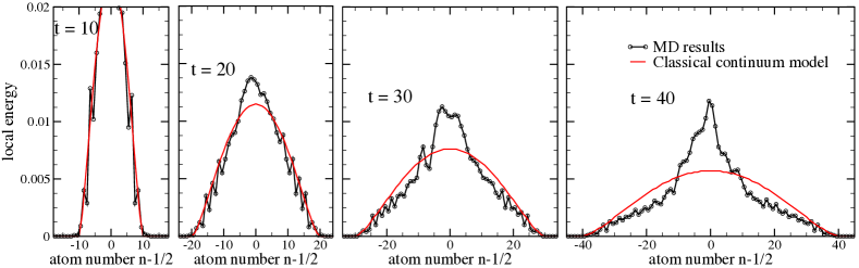
Figure 4: Total energy profile $E_{a}(\ell)$ of a D-pulse at $T=0$, after spreading in the lattice with 10% of the masses increased by 1.5. The profiles are averaged over 100 random realizations of mass disorder. Time is in units $\sqrt{M/K}$. The red curves are the ballistic prediction of Eq. 12. The value of $E_{0}$ has been rescaled from 1 to 0.27, corresponding to $u_{0}=0.3$, which is the value chosen for this and subsequent computations.

Disorder adds an interesting complication to heat conduction in 1-d harmonic crystals Matsuda and Ishii (1970); Visscher (1971), namely Anderson localization Anderson (1958). In disordered metals of dimension 2 or less, ignoring electron-electron interactions, all single-particle electron eigenstates are localized Abrahams et al. (1979). At $T=0$, an electron inserted into a localized state cannot propagate. Localization of phonons is similar Sheng (2005); Kirkpatrick (1985); Luckyanova et al. (2018), except that small $Q$ acoustic phonons have to travel very long distances before localization appears Lepri et al. (2003). Reference Allen and Kelner, 1998 gives the example of a wave packet progating on a weakly mass-disordered chain. Ballistic propagation is seen at short distances and times, diffusive propagation at intermediate ones, and Anderson localization at long distances and times. When $T>0$, interactions with phonons allow a localized electron to hop to neighboring localized states, which causes slow diffusion. Anharmonic interactions have a similar effect Fabian and Allen (1996) on localized phonons in insulators. If disorder is not too great, phonon quasiparticles are a realistic model at intermediate times and distances. Ballistic phonons eventually scatter from disorder and evolve toward diffusive at moderate to long distances and times, before localizing. A perturbative treatment of scattering can likely describe the evolution before localization sets in.

We now add mass defects to allow deviation from ballistic propagation, by randomly choosing 10% of the atoms, and increasing their masses from $M=1$ to $M^{\ast}=1.5$. Results at various times for a D pulse are shown in Fig. 4. The lattice is still harmonic, but the Hamiltonian is no longer diagonal in the plane-wave basis, Eq. 2. Before ensemble averaging, the pulse shape varies depending on the locations of the mass defects relative to the point of pulse insertion. The D-pulse shapes of Fig. 4 have been averaged over 100 different random placements of the altered masses.

The pulse shape at $t=10\sqrt{M/K}$ is not much altered from pure ballistic behavior. The pulse has propagated only a distance of $\pm 10$ atoms, and encountered typically only two impurities. As time proceeds, there is increasing deviation from the ballistic pulse shape predicted in Eq. 12, and shown in the red curves. By $t=40$, the fraction of the energy at distances $<10a$ has failed to diminish the way ballistic propagation does. The energy in the intermediate $10-30$ atoms has diminished more than ballistic propagation does. The crossover toward diffusion is underway. The disorder is weak, so the Anderson localization lengths $\xi_{Q}$ are mostly longer than the propagation distance ($\leq 40a$) studied here.

VII Pure Diffusion

The opposite extreme from ballistic propagation is pure diffusion. The equation for the energy $\Delta E$ propagating diffusively from a pulse $P$ is

$$\left(\frac{\partial}{\partial t}-D\frac{d^{2}}{dr^{2}}\right)\Delta E(r,t)=P(r,t)=E_{0}\delta(r)\delta(t)$$ (24)

This follows from energy conservation, Eq. 15, provided there is a local relation $j=-\kappa dT/dr$ between current $j(r,t)$ and temperature $T(r,t)$. It also uses as the definition of temperature $\Delta E(r,t)=C\Delta T(r,t)$. Then the diffusion constant is $D=\kappa/C$ where $\kappa$ and $C$ are bulk thermal conductivity and specific heat. The solution of Eq. 24 is

$$\Delta E_{\rm diff}(r,t)=\frac{E_{0}}{\sqrt{4\pi Dt}}e^{-r^{2}/4Dt}\theta(t),$$ (25)

where $\theta(t)$ is the Heaviside function.

Pure diffusion is inconsistent with a quasiparticle picture of pulse evolution. One argument is that it violates the rule that lattice vibrational energy cannot propagate faster than the speed of sound $v_{M}$. It is not necessarily a large violation. An estimate of the size uses $\kappa\approx Cv\ell=Cv^{2}\tau$. The diffusive exponent $r^{2}/4Dt$ is then approximately $(t/4\tau)(r/v_{M}t)^{2}$ (where $\ell$ and $\tau$ are rough measures of mean free path and lifetime of phonons). Therefore, when $t=4\tau$, there is some diffusive energy at $r>v_{M}t$, which decays rapidly as $r/v_{M}t$ or $t/4\tau$ increases.

Another argument for the inapplicability of pure diffusion to quasiparticles is that mean free paths of small $Q$ acoustic phonons typically diverge as a power, $\ell_{Q}\propto 1/Q^{p}$, causing $D$ to diverge. This is a correct result, not an error of perturbation theory. A formula for $D=\kappa/C$ is found from the standard RTA solution of Boltzmann theory for $\kappa$ in the bulk limit,

$$D=\frac{\sum_{Q}C_{Q}v_{Q}^{2}\tau_{Q}}{\sum_{Q}C_{Q}}\rightarrow\frac{1}{N}\sum_{Q}v_{Q}^{2}\tau_{Q}.$$ (26)

The second form is the classical limit where $C_{Q}=\hbar\omega_{Q}dn_{Q}/dT\rightarrow k_{B}$. When $1/\tau_{Q}$ arises from mass disorder, the small $Q$ scattering rate $1/\tau_{Q}$ in $d=1$ goes as $(Q^{2})$ Matsuda and Ishii (1970); Li et al. (2014); Rubin and Greer (1971); Verheggen (1979); Dhar (2008), shown explicitly in appendix A. The divergence is not limited to one dimension. Small $Q$ scattering from mass defects is closely analogous to Rayleigh scattering of light from density fluctuations. In 3d, both light and phonon scattering have $Q^{4}$ dependences at small $Q$. The $Q$-sum needed to compute $D$ or $\kappa$ diverges as $1/Q^{2}$ in both $d=1$ and $d=3$, unless another scattering process adds a term to $1/\tau_{Q}$ that blocks the divergence. When $T$ is small enough that mean free paths $\ell_{Q}=v_{Q}\tau_{Q}$ reach sample dimensions $L$, the zero denominator from the diverging defect term becomes non-zero due to boundary scattering $L=v_{Q}\tau_{\rm boundary}$. Glassbrenner and Slack analyze experiments which illustrate this Glassbrenner and Slack (1964). It is seen in clean but isotopically disordered crystals Thacher (1967); Asen-Palmer et al. (1997); Lindsay et al. (2013). Eqn. 26 can be replaced by

$$D=\sum_{Q}v_{Q}^{2}\left[(1/\tau_{Q})_{\rm disorder}+|v_{Q}|/L\right]^{-1}.$$ (27)

The sum now converges, diverging for large $L$ as $D\propto\sqrt{L}$ in $d=1$. The $\sqrt{L}$ scaling of $\kappa$ in d=1 was noticed earlier Matsuda and Ishii (1970); Keller et al. (1978). The resulting $D$ is plotted versus $L/a$ in Fig. 5. Our Newtonian simulation on a loop of 200 atoms has no boundary scattering because of periodic boundary conditions. If we had used instead rough boundaries, then $L$ in Eq. 27 would be $100a$, resulting in $D=35\omega_{M}a^{2}/2$ (see Appendix A).

Figure 5: The diffusivity in bulk RTA theory, from Eq. 27 and 36, using Eq. 28 for the disorder scattering, with the dimensionless strength $\epsilon=1/90$. The diffusivity diverges as $\sqrt{(}L/\epsilon)$ as $L\rightarrow\infty$.

In spite of the inapplicability of Eq. 25, it is interesting to compare it to the numerical results. Figure 6 compares the simulation result of the disordered D-pulse at $t=40$ (the last graph of Fig. 4) with the formulas for pure ballistic and pure diffusive propagation. For the majority of atoms (all but atoms 10-14) the computed pulse energy is closer to the green curve illustrating pure diffusion (with $D=1.8$) than to the red curve of pure ballistic behavior. However, the agreement with pure diffusion is poor, and more important, the choice $D=1.8$ was chosen to give a curve for $\Delta E(r,t=40)$ reasonably close to the simulation, but it is totally unrealistic, corresponding to a nanoscale sample with boundaries at $L\approx\pm 3a$, as seen from Fig. 5.

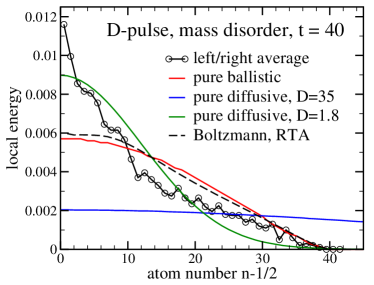
Figure 6: The same $t=40$ pulse energy profile $E_{a}(\ell)$ as in Fig. 4, but showing only $x>0$ and averaging the left and right propagating portions. The red curve is the ballistic prediction of Eq. 12, and the blue curve is the diffusive prediction of Eq. 25, with diffusion constant $D=35a^{2}\omega_{M}/2$ as explained in the text. The green curve is the same, except $D=1.8a^{2}\omega_{M}/2$ is used to make diffusion appear closer to the computed pulse profile. The dashed curve is the Boltzmann prediction (with no boundary scattering) using version (1) of RTA, shown in Eq. 30 and explained in section VIII. All “theoretical” curves are scaled to $E_{0}=0.27$ to agree with the numerical simulation.

VIII Boltzmann theory with mass disorder

How does non-local Boltzmann theory treat pulse shape evolution as altered by disorder? Here we answer this question within the relaxation time approximation (RTA), and find that the results have the correct trend but do not agree closely with simulations. The collision operator $C_{QQ^{\prime}}$ in Eq. LABEL:eq:PBEkw is replaced in RTA by $1/\tau_{Q}\delta_{QQ^{\prime}}$, where $1/\tau_{Q}$ is the diagonal element, $C_{QQ}$,

$$1/\tau_{Q}=\epsilon\omega_{M}\frac{\sin^{2}(Qa/2)}{\cos(Qa/2)}.$$ (28)

This is derived in appendix A, Eq. 35. The RTA solution is a modified version of Eq. 21,

$$\Phi_{Q}(k,\omega)=\frac{-i(kv_{Q}-\omega)\frac{\partial n_{Q}}{\partial T}\Delta T(k,\omega)+\Delta E_{Q}^{\rm ext}/\hbar\omega_{Q}}{1/\tau_{Q}+i(kv_{Q}-\omega)}.$$ (29)

This gives $N$ equations (one for each mode $Q$), for the $N$ unknown functions $\Phi_{Q}(k,\omega)$. There is an additional unknown, the local temperature shift $\Delta T(k,\omega)$. An extra equation, to supplement Eq. 29, is needed.

The requirement of energy conservation says that $\sum_{Q}\hbar\omega_{Q}\left(d\Phi_{Q}/dt\right)_{\rm coll}=0$. The correct scattering operator satisfies this automatically, but the RTA version, $(dE/dt)_{\rm coll,RTA}=-\sum_{Q}\hbar\omega_{Q}\Phi_{Q}/\tau_{Q}=0$, is not automatically satisfied. Forcing $\Phi_{Q}$ to satisfy this equation as well as the linearized PBE is one way to obtain the extra equation needed to determine $\Delta T(k,\omega)$ and $\Delta T(r,t)$. This definition of temperature which we call “version (1)”, is not a normal one. A possible alternative is to define temperature in terms of the local energy, $E(r,t)=\sum_{Q}\hbar\omega_{Q}n_{Q}(T(r,t))$ or $E(k,\omega)=\sum_{Q}\hbar\omega_{Q}(dn_{Q}/dT)\Delta T(k,\omega)$. This, called “version (2)”, is the definition of $\Delta T(k,\omega)$ used in the full Boltzmann equation with the correct scattering operator. It requires the deviation $\Phi_{Q}(r,t)$ to have no net energy. This definition of temperature is quite normal - it is sensible in a quasiparticle theory, although perhaps not demanded by nonequilibrium thermodynamics.

The two possible versions of the extra equation, needed in RTA, are then

$$\bf{(1)}\ \sum_{Q}\frac{\hbar\omega_{Q}\Phi_{Q,{\rm RTA}}}{\tau_{Q}}=0;\ {\rm or}\ {\bf(2)}\ \sum_{Q}\hbar\omega_{Q}\Phi_{Q,{\rm RTA}}=0.$$ (30)

We find that version (1) gives a more realistic answer, in agreement with previous numerical Allen and Perebeinos (2018) and theoretical Vermeersch and Shakouri (2014); Vermeersch et al. (2015); Hua and Minnich (2015) work.

Figure 7: RTA predictions for the total energy profile $E_{a}(\ell)$ of a D-pulse at $t=40$ and $T=0$, after spreading in the lattice with 10% of the masses increased by 1.5. The input energy $E_{0}$ is set to 0.27, for comparison with numerical results. The red and black curves use version (1) of Eq. 30, and the blue curve uses version (2). The total energy (solid curves) correctly agrees with $E_{0}$ in version (1), but in version (2), is smaller by a factor 0.415. In version (1), the thermal energy is (incorrectly, we believe) larger than $E_{0}$ by a factor 1.58.

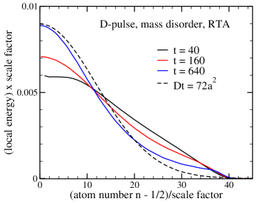
Figure 8: Boltzmann results using RTA, with impurity but no boundary scattering, at three times, $t=$ 40, 160, and 640. Time is in units $2/\omega_{M}=1$. The scale factors 1, 4, and 16 are used to keep the correct area ($E_{0}=0.27$) while scaling the horizontal distance $v_{M}t$ to 40 to make the results fit on a single graph. The dashed line is pure diffusion $\propto\exp(-x^{2}/4Dt)$ (Eq. 25) at $t=40$, with the same arbitrary diffusivity $D=1.8\omega_{M}a^{2}/2$ used in Fig. 6, chosen just to illustrate pure diffusion.

The pulse energy predicted by version (1) is shown in Fig. 6. It deviates less from ballistic than does the simulation, but in the correct direction. Energy profiles predicted by both versions of the RTA Boltzmann theory are in Fig. 7 for the D pulse at $t=40$. Details of the computational proceedure are given in appendix B and in the Supplemental Material Allen and Nghiem . Version (1) of RTA theory correctly keeps the total pulse energy equal to $E_{0}$ as $t$ increases, while version (2) does not. Version (2) has another weakness, namely the predicted shape of the evolving pulse in Fig. 7 is very different from the simulated results in Fig. 6, unlike version (1) where the Boltzmann-RTA pulse shape is sensible. However, version (1) has a temperature profile $\Delta T(r,t)$ in Fig. 7 that differs from $\Delta E(r,t)$ without physical justification, unlike version (2) which correctly equates $k_{B}T(r,t)$ and $\Delta E(r,t)$.

Figure 8 shows version (1) RTA results for long times to illustrate a slow approach toward something related to, but not closely agreeing with, pure diffusion, Eq. 25. The RTA diffusivity $D=1.8$ used in the dashed curve of Fig. 8 uses an unrealistically small sample size, $\approx 6a$,as mentioned already. These results confirm the arguments in Sec. VII that pure diffusion disagrees with quasiparticle theories.

Why do the Boltzmann-RTA results not agree well with the numerical pulse shapes? The reason could be a mixture of two problems: (1) inadequacy of second order Fermi golden rule, related to incipient Anderson localization; and (2) use of RTA instead of correct local energy-conserving scattering.

IX anharmonic

The famous work of Fermi, Pasta, Ulam (FPU) and Tsingou (FPUT) Fermi et al. (1955) found unexpected anomalies in the opposite limit of our pulse propagation, namely the zero temperature behavior of the lowest harmonic normal mode of the fixed-end chain, when forces differ from harmonic by one or the other of two choices for the anharmonic nearest neighbor coupling,

$${\mathcal{H}}_{3}^{\prime}=\frac{V_{3}}{3}\sum_{\ell}(r_{\ell+1}-r_{\ell})^{3}\ \ (V_{3}=\alpha K,\ {\rm the}\ \alpha-{\rm model});$$ (31)

$${\mathcal{H}}_{4}^{\prime}=\frac{V_{4}}{4}\sum_{\ell}(r_{\ell+1}-r_{\ell})^{4}\ \ (V_{4}=\beta K,\ {\rm the}\ \beta-{\rm model}).$$ (32)

Heat conduction in weakly anharmonic linear lattices has been studied Lepri (2000) and reviewed Lukkarinen (2016). Recent work Dematteis et al. (2020); Lepri et al. (2020); Wang et al. (2020) seems to confirm (at least qualitatively) that perturbation theory works in the regime studied here. If so, the perturbative picture says that mean free paths will diminish as T increases Maradudin (1962); Conway (1965). A crossover to diffusive behavior, which FPU indicates might not happen at T = 0, may well happen at $T>0$, at rates that increase as T increases.

We have looked at $T=0$ anharmonic D-pulse propagation, using both third-order ($V_{3}$, also known as “FPU$-\alpha$”) and fourth-order ($V_{4}$, also known as “FPU$-\beta$”) anharmonicity. The coefficients $\alpha$ and $\beta$ in Eqs. 31 and 32 were set to 1. Local energy $E(\ell,t)$ is defined as in Eq. LABEL:eq:Eell: the total (harmonic and anharmonic) potential energy of a spring is assigned half to each neighboring atom. The results are in Fig. 9. The initial pulse ($u_{0,1}=\pm 0.3$) is the same as in previous computations, except the total energy is no longer $0.27E_{0}$ as in previous computations, because there is additional anharmonic energy, $-27\%$ in $V_{3}$ and $+12\%$ in $V_{4}$. The initial pulse has the same harmonic amplitudes $A_{Q}$ and phases $\phi_{Q}$ as previously, but anharmonic terms alter these fairly quickly. As the pulse spreads and $\Delta E(\ell,t)$ spreads out, anharmonic forces diminish. Amplitudes and phases evolve less, becoming more stable. As $t$ increases, local energy propagation from $(x,t)$ reverts more closely to ballistic. This is especially noticable in the $V_{3}$ case, where atoms $10-16$ seem little affected by anharmonic effects. The $V_{3}$ case might be especially difficult to analyze perturbatively, because in lowest order and 1d, anharmonic decay is essentially kinematically forbidden, requiring higher order effects to change $A_{Q}$ and $\phi_{Q}$. It would be interesting to study the anharmonic pulse at finite $T$ where anharmonic effects do not disappear as the pulse propagates.

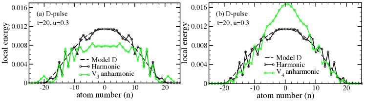
Figure 9: Displacement (D) pulse at time $t=20$ after insertion at $T=0$ and $t=0$. The harmonic ($K_{2}$) force constant is 1. (a) has $V_{3}=1$ and $V_{4}=0$; (b) has $V_{3}=0$ and $V_{4}=1$. The pure harmonic result ($V_{3}=V_{4}=0$) is shown for comparison in both panels. To see the effect of anharmonicity, initial pulse amplitudes on atoms 0 and 1 were given large values, 0.3 and -0.3, respectively. The initial anharmonic energy in (a) is $-0.27\ \times$ the initial harmonic energy ($0.27E_{0}$), and in (b) $+0.12\ \times$ the initial harmonic energy ($0.27E_{0}$).

X conclusions

Time evolution of pulse energy gives useful pictures and insights into non-local phonon transport. The main conclusions are: (1) Different forms of pulse insertions give interestingly diverse pulse energy shapes. (2) Atomistic local energy $E(\ell,t)$ is not uniquely defined and has surprisingly different details when different sensible definitions are used. (3) A continuum picture works well and enables simple formulas for ballistic propagation. (4) A non-local version of Boltzmann theory for the collisionless phonon gas is very successful, and the phonon insertion term $(\partial N_{Q}/\partial t)_{\rm ext}$ has an unambiguous form. (5) Mildly disordered harmonic systems have interesting pulse evolution, but are not well explained by non-local Boltzmann theory in relaxation time approximation (RTA). Ambiguity about temperature definition in RTA is a difficulty; previous ideas are confirmed. (6) Pure diffusion does not work at the local level, when phonon quasiparticles are good approximations, even after long pulse evolution times. (7) The pulse evolution of 1d anharmonic chains at $T>0$ deserves further study.

XI acknowledgements

We are grateful to the Stony Brook Institute for Advanced Computational Science for use of their computer cluster.

Appendix A Phonon relaxation from mass disorder

The Fermi golden rule for phonon decay by defects is $1/\tau_{Q}=(2\pi/\hbar)\sum_{Q\prime}|V_{QQ^{\prime}}|^{2}\delta(\hbar\omega_{Q}-\hbar\omega_{Q^{\prime}})$. When the interaction $V_{QQ^{\prime}}$ arises from mass disorder, the decay rate is

$$\left(\frac{1}{\tau_{Q}}\right)_{\rm imp}=\frac{\pi}{2\hbar}\frac{N_{i}}{N}\left(\frac{\Delta M}{M^{\ast}}\right)^{2}(\hbar\omega_{Q})^{2}\mathcal{D}(\omega_{Q}),$$ (33)

where $\Delta M=M^{\ast}-M$ is the mass difference between impurities ($M^{\ast}$) and pure ($M$) masses, and $N_{i}/N$ is the fraction of impurities. The density of vibrational states of the ordered harmonic chain is

$$\mathcal{D}(\omega)=\frac{1}{\hbar N}\sum_{Q}\delta(\omega-\omega_{Q})=\frac{2}{\pi\hbar}\frac{1}{(\omega_{M}^{2}-\omega^{2})^{1/2}}.$$ (34)

Then the decay rate is

$$\frac{1}{\tau_{Q}}=\epsilon\frac{\omega_{Q}^{2}}{(\omega_{M}^{2}-\omega_{Q}^{2})^{1/2}},\ \ {\rm where}\ \ \epsilon=\frac{N_{i}}{N}\left(\frac{\Delta M}{M^{\ast}}\right)^{2},$$ (35)

and $\epsilon=1/90$ in our simulations.

The formula 27 for boundary-limited diffusivity can be written as

$$D(L)=\frac{\omega_{M}a^{2}}{2}\frac{s}{\pi\epsilon}\int_{0}^{\pi/2}dx\frac{\cos^{3}x}{\cos^{2}x+s\sin^{2}x},$$ (36)

where $s=2L\epsilon/a$ and $\omega_{M}a^{2}/2=1$ is the unit of diffusivity. At large $s$, the diffusivity scales as $\sqrt{s}/\epsilon\propto\sqrt{(}L/\epsilon)$.

Appendix B Solution of Boltzmann equation in RTA

Using Eq. 29 and version (1) of Eq. 30, the equation for $\Delta T$ is

$$k_{B}\Delta T_{(1)}(k,\omega)=\frac{A(k,\omega)}{B(k,\omega)},$$ (37)

where

$$A(k,\omega)=\frac{1}{N}\sum_{Q}\frac{\Delta E_{Q}^{\rm ext}/\tau_{Q}}{1/\tau_{Q}-i(\omega-kv_{Q})},$$ (38)

$$B(k,\omega)=\frac{1}{N}\sum_{Q}\frac{1}{\tau_{Q}}\frac{-i(\omega-kv_{Q})\left[\frac{\hbar\omega_{Q}}{k_{B}}\frac{\partial n_{Q}}{\partial T}\right]}{1/\tau_{Q}-i(\omega-kv_{Q})}.$$ (39)

Once $\Delta T_{(1)}(k,\omega)$ is computed, the corresponding local energy $\Delta E_{(1)}(k,\omega)$ can be found and Fourier transformed to get $\Delta E_{(1)}(r,t)$,

$$\Delta E_{(1)}(k,\omega) \equiv \sum_{Q}\hbar\omega_{Q}\left[N_{Q}-n_{Q}(T_{0})\right]$$ (40)

$$= C(k,\omega)k_{B}\Delta T_{(1)}(k,\omega)+D(k,\omega),$$

where

$$C(k,\omega)=\frac{1}{N}\sum_{Q}\frac{1/\tau_{Q}\left[\frac{\hbar\omega_{Q}}{k_{B}}\frac{\partial n_{Q}}{\partial T}\right]}{1/\tau_{Q}-i(\omega-kv_{Q})},$$ (41)

$$D(k,\omega)=\frac{1}{N}\sum_{Q}\frac{\Delta E_{Q}^{\rm ext}}{1/\tau_{Q}-i(\omega-kv_{Q})}.$$ (42)

The factor in square brackets ($[\ ]$) in Eqs. 39 and 41 (and later in Eq. 45) becomes 1 in the classical limit, which is needed for comparison with the numerical pulse spreading.

To implement version (2), use the simpler condition

$$\Delta E_{(2)}(k,\omega)=k_{B}\Delta T_{(2)}(k,\omega).$$ (43)

Using Eq. 29 and version (2) of Eq. 30, the equation for $\Delta E$ is

$$\Delta E_{(2)}(k,\omega)=k_{B}\Delta T_{(2)}(k,\omega)=\frac{D(k,\omega)}{F(k,\omega)},$$ (44)

where, except for omission of factors of $1/\tau_{Q}$ in the numerator, $D(k,\omega)$ is the same as $A(k,\omega)$ and $F(k,\omega)$ is the same as $B(k,\omega)$. To be explicit,

$$F(k,\omega)=\frac{1}{N}\sum_{Q}\frac{-i(\omega-kv_{Q})\left[\frac{\hbar\omega_{Q}}{k_{B}}\frac{\partial n_{Q}}{\partial T}\right]}{1/\tau_{Q}-i(\omega-kv_{Q})}.$$ (45)

Details of the numerical calculations, especially the difficult Fourier transforms needed to get pulse shapes in $(x,t)$-space, are in the Supplemental Materials Allen and Nghiem .

Appendix C Laplace transform method of Vermeersch et al.

Vermeersch et al. (Ref. Vermeersch et al., 2015) used mixed Fourier (for space variables $r\leftrightarrow k$) and Laplace (for time variables $t\leftrightarrow\omega$) transforms to solve for the case of a V1 pulse in one dimension. They used version (1) of Eq. 30, but did not transform from $(k,\omega)$ to $(r,t)$. However, they found interesting identities in Laplace space, which we will here pursue for arbitary $E_{Q}^{\rm ext}$, not just the V1 choice $E_{Q}^{\rm ext}=E_{0}/N$. The basis for their identities are the Fourier equations

$$\frac{1}{N}\sum_{r}F(r,t)=\left[F(k,t)\right]_{k=0},$$ (46)

$$\frac{1}{N}\sum_{r}r^{2}F(r,t)=-\left[\frac{d^{2}}{dk^{2}}F(k,t)\right]_{k=0}.$$ (47)

Together, these give a result for a mean square displacement

$$\langle r^{2}\rangle_{F}=\frac{\sum_{r}r^{2}F(r,t)}{\sum_{r}F(r,t)},$$ (48)

where $F$ is an arbitrary distribution.

When the time variable is transformed to Laplace space rather than Fourier space, $\Phi_{Q}(r,\omega)$ becomes $\int_{0}^{\infty}dt\exp(-\omega t)\Phi_{Q}(r,t)$. The symbol $\omega$ previously used for the Fourier variable is now used for the Laplace variable. The solution of the Boltzmann equation is then exactly the same as previously, Eqns. 37 and 40, except that the Fourier variable $-i\omega$ becomes the Laplace variable $\omega$. Using the fact that sums over $Q$ contains pairs $Q$ and $-Q$ with $v_{-Q}=-v_{Q}$, which causes imaginary parts to vanish, and using the notations $C_{Q}=\hbar\omega_{Q}dn_{Q}/dT$ and $\Lambda_{Q}=v_{Q}\tau_{Q}$, the functions that determine $\Delta T(k,\omega)$ and $\Delta E(k,\omega)$ are

$$A(k,\omega)=\frac{1}{N}\sum_{Q}\frac{\Delta E_{Q}^{\rm ext}(1+\omega\tau_{Q})}{(1+\omega\tau_{Q})^{2}+(k\Lambda_{Q})^{2}},$$ (49)

$$B(k,\omega)=\frac{1}{N}\sum_{Q}\frac{C_{Q}}{\tau_{Q}}\left[1-\frac{(1+\omega\tau_{Q})}{(1+\omega\tau_{Q})^{2}+(k\Lambda_{Q})^{2}}\right],$$ (50)

$$C(k,\omega)=\frac{1}{N}\sum_{Q}\frac{C_{Q}(1+\omega\tau_{Q})}{(1+\omega\tau_{Q})^{2}+(k\Lambda_{Q})^{2}},$$ (51)

$$D(k,\omega)=\frac{1}{N}\sum_{Q}\frac{\Delta E_{Q}^{\rm ext}\tau_{Q}(1+\omega\tau_{Q})}{(1+\omega\tau_{Q})^{2}+(k\Lambda_{Q})^{2}}.$$ (52)

Then recalling that $\Delta T(k,\omega)=A(k,\omega)/B(k,\omega)$, Eqs. 49 and 50 give Eq. 4 of Vermeersch et al. in the V1 case. They use $C_{Q}\rightarrow k_{B}$, the classical limit, and set $E_{Q}^{\rm ext}=E_{0}\rightarrow 1$ (which they call a unit pulse). The general answer for the integrated temperature rise of a pulse is

$$d_{T}(\omega)\equiv\frac{1}{N}\sum_{r}\Delta T(r,\omega)=\frac{1}{\omega}\frac{\sum_{Q}\frac{\Delta E_{Q}^{\rm ext}}{1+\omega\tau_{Q}}}{\sum_{Q}\frac{C_{Q}}{1+\omega\tau_{Q}}}.$$ (53)

For the V1 pulse in the classical limit, this gives the total pulse temperature rise as $\sum_{r}k_{B}\Delta T(r,\omega)=E_{0}/\omega$. Then the inverse Laplace transform gives the result of Ref. Vermeersch et al., 2015, $\sum_{r}k_{B}\Delta T(r,t)=E_{0}$. However, for other pulse forms of $E_{Q}^{\rm ext}$, there is no analytic inverse Laplace transform of Eq. 53. Also, Vermeersch et al. incorrectly identify $\sum_{r}k_{B}\Delta T(r,t)$ with the pulse energy $\sum_{r}\Delta E(r,t)$. This identification is version (2) of Eq. 30, but is inconsistent with version (1) which they (sensibly) adopt as the preferred RTA approximation. Fortunately, the erroneous identification of $\Delta E(r,t)$ with $k_{B}\Delta T(r,t)$ goes away in the V1 case when summed over all $r$. Using the correct RTA version

$$\Delta E(k,\omega)=k_{B}\frac{A(k,\omega)}{B(k,\omega)}C(k,\omega)+D(k,\omega),$$ (54)

gives the result

$$\Delta E(k=0,\omega)=\frac{1}{\omega N}\sum_{Q}\Delta E_{Q}^{\rm ext}=\frac{E_{0}}{\omega}$$ (55)

for all $\Delta E_{Q}^{\rm ext}$, not just the V1 case. Doing the inverse Laplace transform then shows that the RTA in version (1) correctly conserves the pulse energy in time,

$$\sum_{r}\Delta E(r,t)_{RTA,(1)}=E_{0},$$ (56)

not just for the V1 pulse, but for arbitrary choice of $\Delta E_{Q}^{\rm ext}$. This is not surprising; version (1) of Eq. 30 enforces overall energy conservation in RTA. Version (2) does not and does not obey Eq. 56. The Vermeersch et al. identification of $\Delta E(k,\omega)$ with $k_{B}\Delta T(k,\omega)$ is correct in the $k=0$ limit, but only for the V1 pulse, not for others.

Now examine the mean square displacements, using Eq. 47. For the case $\Delta T(k,\omega)=A(k,\omega)/B(k,\omega)$, the answer in Laplace space is

$$n_{T}(\omega) \equiv \frac{1}{N}\sum_{r}r^{2}\Delta T(r,\omega)=2\frac{\sum_{Q}\frac{\Delta E_{Q}^{\rm ext}\Lambda_{Q}^{2}}{(1+\omega\tau_{Q})^{3}}}{\sum_{Q}\frac{\omega C_{Q}}{(1+\omega\tau_{Q})}}$$ (57)

$$+ 2\frac{\sum_{Q}\frac{\Delta E_{Q}^{\rm ext}}{(1+\omega\tau_{Q})}}{\left[\sum_{Q}\frac{\omega C_{Q}}{(1+\omega\tau_{Q})}\right]^{2}}\sum_{Q}\frac{C_{Q}\Lambda_{Q}^{2}/\tau_{Q}}{(1+\omega\tau_{Q})^{3}}$$

For the V1 pulse this simplifies to

$$\frac{1}{N}\sum_{r}r^{2}\Delta T(r,\omega)=\frac{2}{\omega^{2}}\frac{\sum_{Q}\frac{C_{Q}\Lambda_{Q}^{2}/\tau_{Q}}{(1+\omega\tau_{Q})^{2}}}{\sum_{Q}\frac{C_{Q}}{(1+\omega\tau_{Q})}},$$ (58)

which is Eq. 6 of Vermeersch et al..

The point of these calculations is that in principle we could do inverse Laplace transforms to get $n_{T}(t)$ from $n_{T}(\omega)$ and $d_{T}(t)$ from $d_{T}(\omega)$, and then take their ratio $n_{T}(t)/d_{T}(t)$ to get the mean square displacement $\langle r^{2}(t)\rangle_{T}$ of the pulse temperature profile $\Delta T(r,t)$. Analytic inversions are not available. Vermeersch et al. instead look at the limit of high $\omega\tau_{Q}$ which should give $\langle r^{2}(t)\rangle_{T}$ at small times $t$, and also at the limit of low $\omega\tau_{Q}$ which should give $\langle r^{2}(t)\rangle_{T}$ at large times $t$.

At large $\omega\tau_{Q}$, the $\omega$-dependences of $n_{T}(\omega)$ and $d_{T}(\omega)$ are

$$\frac{1}{N}\sum_{r}r^{2}\Delta T(r,\omega)\rightarrow \frac{2}{\omega^{3}}\sum_{Q}[\Delta E_{Q}^{\rm ext}/\tau_{Q}]v_{Q}^{2}/\sum_{Q}[C_{Q}/\tau_{Q}]$$ (59)

$$+{\mathcal{O}}\left(\frac{1}{\omega^{4}}\right),$$

$$\frac{1}{N}\sum_{r}\Delta T(r,\omega)\rightarrow \frac{1}{\omega}\sum_{Q}[\Delta E_{Q}^{\rm ext}/\tau_{Q}]/\sum_{Q}[C_{Q}/\tau_{Q}]$$ (60)

$$+{\mathcal{O}}\left(\frac{1}{\omega^{2}}\right).$$

The inverse Laplace transform of $2/\omega^{3}$ is $t^{2}$, and of $1/\omega$ is $1$. Then we get ballistic behavior in the short time limit,

$$\langle r^{2}\rangle_{T}\rightarrow\langle v^{2}\rangle_{T}t^{2}$$ (61)

where the mean square velocity of the temperature pulse is

$$\langle v^{2}\rangle_{T}\rightarrow\sum_{Q}[\Delta E_{Q}^{\rm ext}/\tau_{Q}]v_{Q}^{2}/\sum_{Q}[\Delta E_{Q}^{\rm ext}/\tau_{Q}].$$ (62)

This agrees with Eq. 8 of Vermeersch et al. in the V1 case. It also resembles our result for the collisionless energy pulse propagation, namely Eqs. 9 or 23 plus Eq. 13. However, in contrast with the collisionless limit, there is an extra $Q$ and $T$-dependent factor $1/\tau_{Q}$ in the weights of $\langle v^{2}\rangle$ in Eq. 62. This is clearly wrong; collisions cannot alter the free phonon ballistic propagation velocity at short times when few or no collisions occur.

At small $\omega\tau_{Q}$, the $\omega$-dependences of $n_{T}(\omega)$ and $d_{T}(\omega)$ are

$$\frac{1}{N}\sum_{r}r^{2}\Delta T(r,\omega)\rightarrow \frac{2}{\omega^{2}}\frac{[\sum_{Q}\Delta E_{Q}^{\rm ext}][\sum_{Q}C_{Q}\Lambda_{Q}^{2}/\tau_{Q}]}{[\sum_{Q}C_{Q}]^{2}}$$ (63)

$$+{\mathcal{O}}\left(\frac{1}{\omega}\right),$$

$$\frac{1}{N}\sum_{r}\Delta T(r,\omega)\rightarrow \frac{1}{\omega}[\sum_{Q}\Delta E_{Q}^{\rm ext}]/[\sum_{Q}C_{Q}]$$ (64)

$$+{\mathcal{O}}(1).$$

The inverse Laplace transform of $2/\omega^{2}$ is $2t$, and of $1/\omega$ is $1$. Then we get diffusive behavior in the long time limit,

$$\langle r^{2}\rangle_{T}\rightarrow 2Dt,\ \ {\rm where}\ \ D=\kappa/C$$

$$\kappa=\sum_{Q}C_{Q}\Lambda_{Q}^{2}/\tau_{Q}\ \ {\rm and}\ \ C=\sum_{Q}C_{Q}.$$ (65)

This result is independent of how the pulse inserts energy $\Delta E_{Q}^{\rm ext}$, and the diffusivity $D$ has the correct macroscopic value. This contradicts the argument that pure diffusion isn’t in the nonlocal PBE.

Why would the nonlocal PBE give correct long time diffusion but incorrect short time ballistic? The answer, we think, is that version (1) of RTA, namely energy conservation $\sum_{Q}\hbar\omega_{Q}\Phi_{Q}/\tau_{Q}$ doesn’t work when $\tau_{Q}\rightarrow\infty$.

References

- Liu et al. (2014) Sha Liu, P. Hänggi, Nianbei Li, Jie Ren, and Baowen Li, “Anomalous heat diffusion,” Phys. Rev. Lett. 112, 040601 (2014).
- Vermeersch et al. (2015) B. Vermeersch, J. Carrete, N. Mingo, and A. Shakouri, “Superdiffusive heat conduction in semiconductor alloys. I. Theoretical foundations,” Phys. Rev. B 91, 085202 (2015).
- Hua and Lindsay (2020) Chengyun Hua and L. Lindsay, “Space-time dependent thermal conductivity in nonlocal thermal transport,” Phys. Rev. B 102, 104310 (2020).
- Hua et al. (2017) Chengyun Hua, Xiangwen Chen, N. K. Ravichandran, and A. J. Minnich, “Experimental metrology to obtain thermal phonon transmission coefficients at solid interfaces,” Phys. Rev. B 95, 205423 (2017).
- Hardy (1963) R. J. Hardy, “Energy-flux operator for a lattice,” Phys. Rev. 132, 168–177 (1963).
- Marcolongo et al. (2016) A. Marcolongo, P. Umari, and S. Baroni, “Microscopic theory and quantum simulation of atomic heat transport,” Nature Physics 12, 80 – 84 (2016).
- Ercole et al. (2016) L. Ercole, A. Marcolongo, P. Umari, and S. Baroni, “Gauge invariance of thermal transport coefficients,” J. Low Temp. Phys. 185, 79–86 (2016).
- (8) P. B. Allen and N. A. Nghiem, “Supplemental material for nonlocal phonon heat transport seen in 1-d pulses,” .
- Lindsay et al. (2019) L. Lindsay, A. Katre, A. Cepellotti, and N. Mingo, “Perspective on ab initio phonon thermal transport,” J. Appl. Phys. 126, 050902 (2019).
- Simons (1960) S. Simons, “The Boltzmann equation for a bounded medium I. General theory,” Phil. Trans. Roy. Soc. London, Series A, Math. Phys. Sci. 253, 137–184 (1960).
- Guyer and Krumhansl (1966) R. A. Guyer and J. A. Krumhansl, “Solution of the linearized phonon Boltzmann equation,” Phys. Rev. 148, 766–778 (1966).
- Mahan and Claro (1988) G. D. Mahan and F. Claro, “Nonlocal theory of thermal conductivity,” Phys. Rev. B 38, 1963–1969 (1988).
- Johnson et al. (2013) J. A. Johnson, A. A. Maznev, J. Cuffe, J. K. Eliason, A. J. Minnich, T. Kehoe, C. M. Sotomayor Torres, G. Chen, and K. A. Nelson, “Direct measurement of room-temperature nondiffusive thermal transport over micron distances in a silicon membrane,” Phys. Rev. Lett. 110, 025901 (2013).
- Koh et al. (2014) Yee Kan Koh, D. G. Cahill, and Bo Sun, “Nonlocal theory for heat transport at high frequencies,” Phys. Rev. B 90, 205412 (2014).
- Hua and Minnich (2014a) Chengyun Hua and A. J. Minnich, “Transport regimes in quasiballistic heat conduction,” Phys. Rev. B 89, 094302 (2014a).
- Hua and Minnich (2014b) Chengyun Hua and A. J. Minnich, “Analytical Green’s function of the multidimensional frequency-dependent phonon Boltzmann equation,” Phys. Rev. B 90, 214306 (2014b).
- Hu et al. (2015) Yongjie Hu, Lingping Zeng, A. J. Minnich, M. S. Dresselhaus, and G. Chen, “Spectral mapping of thermal conductivity through nanoscale ballistic transport,” Nature Nanotech. 10, 701 (2015).
- Hua and Minnich (2018) Chengyun Hua and A. J. Minnich, “Heat dissipation in the quasiballistic regime studied using the Boltzmann equation in the spatial frequency domain,” Phys. Rev. B 97, 014307 (2018).
- Hua et al. (2019) Chengyun Hua, L. Lindsay, Xiangwen Chen, and A. J. Minnich, “Generalized Fourier’s law for nondiffusive thermal transport: Theory and experiment,” Phys. Rev. B 100, 085203 (2019).
- Hua (2020) Chengyun Hua, “Phonon mean free path spectroscopy: theory and experiments,” in Nanoscale Energy Transport: Emerging phenomena, methods and applications, edited by Bolin Liao (IOP Publishing, 2020).
- Beardo et al. (2021) A. Beardo, J. L. Knobloch, L. Sendra, J. Bafaluy, T. D. Frazer, Weilun Chao, J. N. Hernandez-Charpak, H. C. Kapteyn, B. Abad, M. M. Murnane, F. X. Alvarez, and J. Camacho, “A general and predictive understanding of thermal transport from 1d- and 2d-confined nanostructures: Theory and experiment,” ACS Nano 15, 13019–13030 (2021).
- Peierls (1929) R. E. Peierls, “Zur kinetischen Theorie der Wärmeleitung in Kristallen,” Ann. Phys. 395, 1055–1101 (1929).
- Horie and Krumhansl (1964) C. Horie and J. A. Krumhansl, “Boltzmann equation in a phonon system,” Phys. Rev. 136, A1397–A1407 (1964).
- Götze and Michel (1967) W. Götze and K. H. Michel, “Two-fluid transport equations for lattices,” Phys. Rev. 157, 738–743 (1967).
- Klein and Wehner (1969) R. Klein and R. K. Wehner, “Derivation of transport equations for anharmonic lattices,” Physik der kondensierten Materie 10, 1–20 (1969).
- Ranninger (1967) J. Ranninger, “Thermal conductivity in nonconducting crystals,” Annals of Physics 45, 452–478 (1967).
- Spohn (2006) H. Spohn, “The phonon Boltzmann equation, properties and link to weakly anharmonic lattice dynamics,” J. Stat. Phys. 124, 1041 – 1104 (2006).
- Vermeersch and Shakouri (2014) B. Vermeersch and A. Shakouri, “Nonlocality in microscale heat conduction,” ArXiv e-prints (2014), arXiv:1412.6555v2 .
- Hua and Minnich (2015) Chengyun Hua and A. J. Minnich, “Semi-analytical solution to the frequency-dependent Boltzmann transport equation for cross-plane heat conduction in thin films,” J. Appl. Phys. 117, 175306 (2015).
- Matsuda and Ishii (1970) H. Matsuda and K. Ishii, “Localization of normal modes and energy transport in the disordered harmonic chain,” Prog. Theor. Phys. Supplement 45, 56–86 (1970).
- Visscher (1971) W. M. Visscher, “Localization of normal modes and energy transport in the disordered harmonic chain,” Prog. Theor. Phys. 46, 729–736 (1971).
- Anderson (1958) P. W. Anderson, “Absence of diffusion in certain random lattices,” Phys. Rev. 109, 1492–1505 (1958).
- Abrahams et al. (1979) E. Abrahams, P. W. Anderson, D. C. Licciardello, and T. V. Ramakrishnan, “Scaling theory of localization: Absence of quantum diffusion in two dimensions,” Phys. Rev. Lett. 42, 673–676 (1979).
- Sheng (2005) Ping Sheng, Introduction to Wave Scattering, Localization and Mesoscopic Phenomena, edition (Springer, Berlin, 2005).
- Kirkpatrick (1985) T. R. Kirkpatrick, “Localization of acoustic waves,” Phys. Rev. B 31, 5746–5755 (1985).
- Luckyanova et al. (2018) M. N. Luckyanova, J. Mendoza, H. Lu, B. Song, S. Huang, J. Zhou, M. Li, Y. Dong, H. Zhou, J. Garlow, L. Wu, B. J. Kirby, A. J. Grutter, A. A. Puretzky, Y. Zhu, M. S. Dresselhaus, A. Gossard, and G. Chen, “Phonon localization in heat conduction,” Science Advances 4, 9460:1–10 (2018).
- Lepri et al. (2003) Stefano Lepri, Roberto Livi, and Antonio Politi, “Thermal conduction in classical low-dimensional lattices,” Physics Reports 377, 1–80 (2003).
- Allen and Kelner (1998) P. B. Allen and J. Kelner, “Evolution of a vibrational wave packet on a disordered chain,” Am. J. Phys. 66, 497–506 (1998).
- Fabian and Allen (1996) J. Fabian and P. B. Allen, “Anharmonic decay of vibrational states in amorphous silicon,” Phys. Rev. Lett. 77, 3839–3842 (1996).
- Li et al. (2014) Wu Li, J. Carrete, N. A. Katcho, and N. Mingo, “ShengBTE: A solver of the Boltzmann transport equation for phonons,” Comp. Phys. Commun. 185, 1747 – 1758 (2014).
- Rubin and Greer (1971) R. J. Rubin and W. L. Greer, “Abnormal lattice thermal conductivity of a one-dimensional, harmonic, isotopically disordered crystal,” J. Math. Phys. 12, 1686–1701 (1971).
- Verheggen (1979) T. Verheggen, “Transmission coefficient and heat conduction of a harmonic chain with random masses: Asymptotic estimates on products of random matrices,” Commun. Math. Phys. 68, 69–82 (1979).
- Dhar (2008) A. Dhar, “Heat transport in low-dimensional systems,” Advances in Physics 57, 457–537 (2008).
- Glassbrenner and Slack (1964) C. J. Glassbrenner and G. A. Slack, “Thermal conductivity of silicon and germanium from 3K to the melting point,” Phys. Rev. 134, A1058–A1069 (1964).
- Thacher (1967) P. D. Thacher, “Effect of boundaries and isotopes on the thermal conductivity of LiF,” Phys. Rev. 156, 975–988 (1967).
- Asen-Palmer et al. (1997) M. Asen-Palmer, K. Bartkowski, E. Gmelin, M. Cardona, A. P. Zhernov, A. V. Inyushkin, A. Taldenkov, V. I. Ozhogin, K. M. Itoh, and E. E. Haller, “Thermal conductivity of germanium crystals with different isotopic compositions,” Phys. Rev. B 56, 9431–9447 (1997).
- Lindsay et al. (2013) L. Lindsay, D. A. Broido, and T. L. Reinecke, “Phonon-isotope scattering and thermal conductivity in materials with a large isotope effect: A first-principles study,” Phys. Rev. B 88, 144306 (2013).
- Keller et al. (1978) J. B. Keller, G. C. Papanicolaou, and J. Weilenmann, “Heat conduction in a one-dimensional random medium,” Commun. Pure Appl. Math. 31, 583–592 (1978).
- Allen and Perebeinos (2018) P. B. Allen and V. Perebeinos, “Temperature in a Peierls-Boltzmann treatment of nonlocal phonon heat transport,” Phys. Rev. B 98, 085427 (2018).
- Fermi et al. (1955) E. Fermi, J. Pasta, and S. Ulam, “Studies of the nonlinear problems, I,” Los Alamos Report LA-1940 (1955), later published in Collected Papers of Enrico Fermi, ed. E. Segre, Vol. II (University of Chicago Press, 1965) p.978; also reprinted in Nonlinear Wave Motion, ed. A. C. Newell, Lecture Notes in Applied Mathematics, Vol. 15 (AMS, Providence, RI, 1974), also in Many-Body Problems, ed. D. C. Mattis (World Scientific, Singapore, 1993).
- Lepri (2000) S. Lepri, “Memory effects and heat transport in one-dimensional insulators,” Eur. Phys. J. B 18, 441–446 (2000).
- Lukkarinen (2016) J. Lukkarinen, “Kinetic theory of phonons in weakly anharmonic particle chains,” in Thermal Transport in Low Dimensions: From Statistical Physics to Nanoscale Heat Transfer, edited by S. Lepri (Springer, Cham, Switzerland, 2016) pp. 159–214.
- Dematteis et al. (2020) G. Dematteis, L. Rondoni, D. Proment, F. De Vita, and M. Onorato, “Coexistence of ballistic and Fourier regimes in the Fermi-Pasta-Ulam-Tsingou lattice,” Phys. Rev. Lett. 125, 024101 (2020).
- Lepri et al. (2020) Stefano Lepri, Roberto Livi, and Antonio Politi, “Too close to integrable: Crossover from normal to anomalous heat diffusion,” Phys. Rev. Lett. 125, 040604 (2020).
- Wang et al. (2020) Jianjin Wang, Sergey V. Dmitriev, and Daxing Xiong, “Thermal transport in long-range interacting Fermi-Pasta-Ulam chains,” Phys. Rev. Research 2, 013179 (2020).
- Maradudin (1962) A. A. Maradudin, “On the lifetime of phonons in one-dimensional crystals,” Phys. Lett. 2, 298–300 (1962).
- Conway (1965) J. Conway, “Decay rate of phonons in a 1-dimensional crystal,” Phys. Lett. 17, 23–24 (1965).