Uncertainty Characteristics Curves: A Systematic Assessment of Prediction Intervals

Abstract

Accurate quantification of model uncertainty has long been recognized as a fundamental requirement for trusted AI. In regression tasks, uncertainty is typically quantified using prediction intervals calibrated to a specific operating point, making evaluation and comparison across different studies difficult. Our work leverages: (1) the concept of operating characteristics curves and (2) the notion of a gain over a simple reference, to derive a novel operating point agnostic assessment methodology for prediction intervals. The paper describes the corresponding algorithm, provides a theoretical analysis, and demonstrates its utility in multiple scenarios. We argue that the proposed method addresses the current need for comprehensive assessment of prediction intervals and thus represents a valuable addition to the uncertainty quantification toolbox.

1 Introduction

The ability to quantify the uncertainty of a model is one of the fundamental requirements in trusted, safe, and actionable AI Arnold et al. (2019); Jiang et al. (2018); Begoli et al. (2019). Numerous methods of generating uncertainty bounds (referred to as prediction intervals, or error bounds) have been proposed in statistics and machine learning literature.

Evaluating the quality of uncertainty bounds, however, remains challenging. While metrics such as the measure of coverage and the likelihood are popular, they conflate the quality of the prediction intervals (PI) with the difficulty of the predictive task at hand. These metrics may be too optimistic (pessimistic) for trivial (challenging) datasets with an easily predictable (hard to quantify) uncertainty and can lead to misleading conclusions. Moreover, tools to compare multiple models producing bounds across different operating points (OP) are scarce. We contend that to measure the quality of uncertainty bounds reliably, we need tools that are both OP and dataset independent.

OP independence. The importance of OP-independent (OP-comprehensive) evaluation metrics is well understood, as demonstrated by techniques such as ROC curves Fawcett (2006) becoming standard practice in numerous areas of AI involving classification, detection, and other tasks. In the context of PI, we define the term OP loosely as a specific setting producing a certain value of either mean coverage or bandwidth (a formal definition will be given in Section 2.3). However, most evaluations of prediction intervals are still performed in a OP-dependent way, evaluating the quality at one (or a small number of) operating point(s).

Dataset independence When possible, metrics should capture the effectiveness of the technique being evaluated, rather than characterize the underlying dataset used in the evaluation. Techniques that contextualize a measurement by comparing it to an intuitive reference offer themselves to address this challenge (for instance, the well-known coefficient of determination, or $R^{2}$, in statistics Steel and Torrie (1960) expresses an observed variance relative to an overall variance to be explained, thus yielding a measure comparable across datasets as well as algorithms).

This paper proposes a methodology for evaluating prediction intervals that addresses both of these issues. First, we introduce the Uncertainty Characteristics Curve (UCC), which leverages the well known concepts of operating characteristic curves to enable OP-independent evaluation. Second, we introduce the notion of a gain over a simple reference, which more intuitively captures the quality of a prediction interval and makes it comparable across different models. These two approaches can be combined to produce a novel metric that we believe is a valuable addition to the prediction interval assessment toolbox.

The contributions of this paper are summarized as follows:

• Developing the Uncertainty Characteristics Curve (UCC) as a tool to comprehensively assess the quality of prediction intervals, whether Bayesian or frequentist in nature.

• Providing a probabilistic interpretation of the area under the UCC.

• Proposing a gain metric that allows for a cross-model comparison.

• Releasing the corresponding code to the research community.

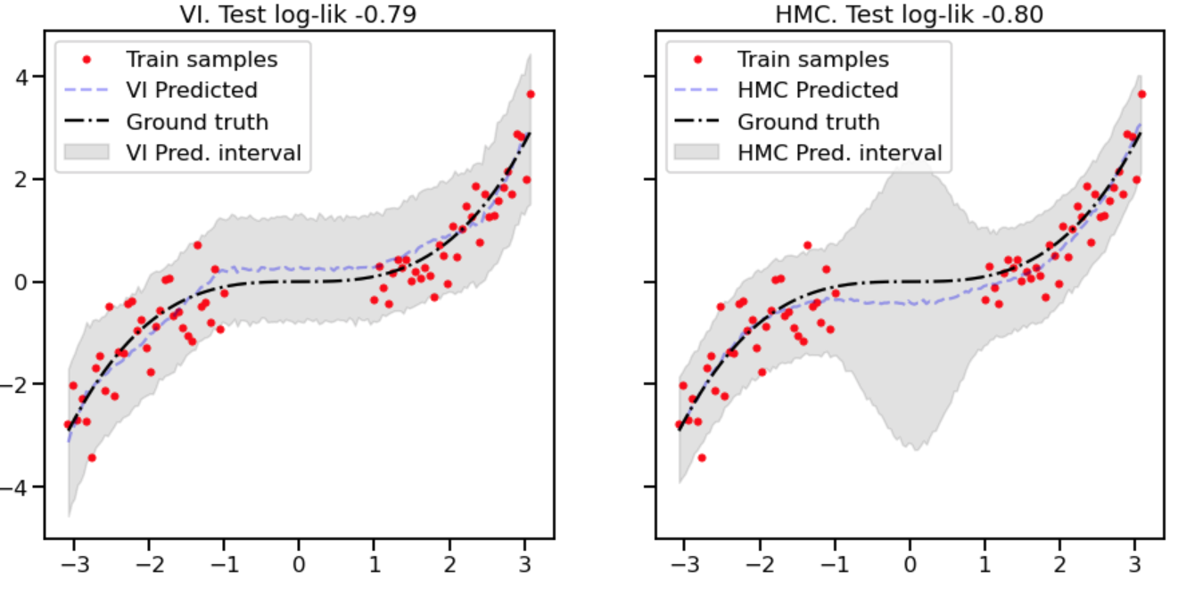
Figure 1: Bayesian Neural Networks applied to a synthetic regression task: Variational Inference (VI) on the left and Hamiltonian Monte Carlo (HMC) on the right. The HMC obtains a lower likelihood.

We want to briefly introduce an illustrative example to underscore the complexities in prediction interval assessment. Figure 1 shows an application of a Bayesian Neural Network (BNN) to a one-dimensional synthetic regression task involving a data gap in the region $[-1,1]$, similar to Yao et al. (2019). The example uses two inference variants to approximate the intractable BNN posterior: a computationally efficient black-box variational inference (VI) and a Hamiltoninan Monte Carlo (HMC) method - largely considered the gold standard for BNN inferenceNeal et al. (2011); Foong et al. (2020). A significant widening in the uncertainty occurs with the HMC in the data-gap region, which appeals to our intuition. However, when assessing the quality using the log-likelihood on test data, the VI scores higher than the HMC - an example of how likelihood may be an inconclusive or a misleading indicator. We will return to this example in more detail later on and show that our proposed metric points clearly in favor of the HMC variant.

2 Method

2.1 Basic Metrics

Suppose there are two components of a model, one generating target predictions, the other assigning uncertainty bounds associated with each such target. Let $V=[Y,\hat{Y},\hat{Y}^{l},\hat{Y}^{u}]^{T}\in\mathbb{R}^{4}$ denote a multivariate random variable comprising the ground truth, $Y$, the target prediction, $\hat{Y}$, the lower uncertainty bound, $\hat{Y}^{l}=\hat{Y}-\hat{Z}^{l}$, and the upper uncertainty bound, $\hat{Y}^{u}=\hat{Y}+\hat{Z}^{u}$. The variables $\hat{Z}^{l},\hat{Z}^{u}$ refer to the predicted uncertainty bands, i.e., the positive deviates from $\hat{Y}$. For simplicity we assume the task involves one-dimensional output, however, all subsequent explanations readily generalize to a multi-dimensional setting. Let $p_{V}$ denote the probability density of $V$ and $\mathbf{v}=\{v_{1},...,v_{N}\}$ a set of $N$ samples from $p_{V}$, where $v_{i}=[y_{i},\hat{y}_{i},\hat{y}_{i}^{l},\hat{y}_{i}^{u}]^{T}$.

We need to consider two cost aspects arising in the assessment of prediction intervals, roughly speaking: (1) what is the extent of observations falling outside the uncertainty bounds (miss rate), and (2) the width of the bounds. An optimal bound captures all of the ground truth (or a calibrated fraction thereof) while being least excessive in terms of its average bandwidth. We define the following metrics as expectations (and their corresponding empirical estimates):

$$\mbox{Miss rate: }\qquad\rho(V)=\operatorname{\mathbb{E}}_{p_{V}}\left[\mathbf{1}_{Y\notin[\hat{Y}^{l},\hat{Y}^{u}]}\right]\,,\qquad\hat{\rho}(\mathbf{v})=\frac{1}{N}\sum_{i:y_{i}\notin[\hat{y}_{i}^{l},\hat{y}_{i}^{u}]}1$$ (1)

$$\mbox{Bandwidth: }\qquad\beta(V)=\frac{1}{2}\operatorname{\mathbb{E}}_{p_{V}}\left[\hat{Y}^{u}-\hat{Y}^{l}\right]\,,\qquad\hat{\beta}(\mathbf{v})=\frac{1}{2N}\sum_{i=1}^{N}\hat{y}_{i}^{u}-\hat{y}_{i}^{l}$$ (2)

Note that $\rho(V)$ is the complement of the well-known Prediction Interval Coverage Probability (PICP) and the bandwidth is half of the Mean Prediction Interval Width (MPIW). In Appendix 9, we define two additional metrics also suitable for practical applications. In favor of coordinate axes consistency, all metrics are defined as costs (hence our choice of Miss Rate over the PICP).

In case the variables $Y,\hat{Y},\hat{Z}^{l}$, and $\hat{Z}^{u}$ are multi-dimensional, the above metrics may be calculated as averages over the individual dimensions.

2.2 Relative Gain

While we want to assess the quality of the uncertainty, most standard metrics (e.g., likelihood, bandwidth, etc.) compound uncertainty bands with actual target predictions. As a consequence, these metrics, in their raw form, are not comparable across different predictors (an example of such confounding is the log-likelihood loss, see Appendix). To address this issue, we look for a relative gain of the PI metrics over some simple, intuitive reference. A good choice of such a reference are constant bands, i.e. $\forall i:\hat{z}_{i}^{l}=const,\hat{z}_{i}^{u}=const$. Given target predictions, $\hat{y_{i}}$, such a non-informative (null) baseline is always possible to generate.

Figure 2 illustrates the issues in comparing raw metrics.

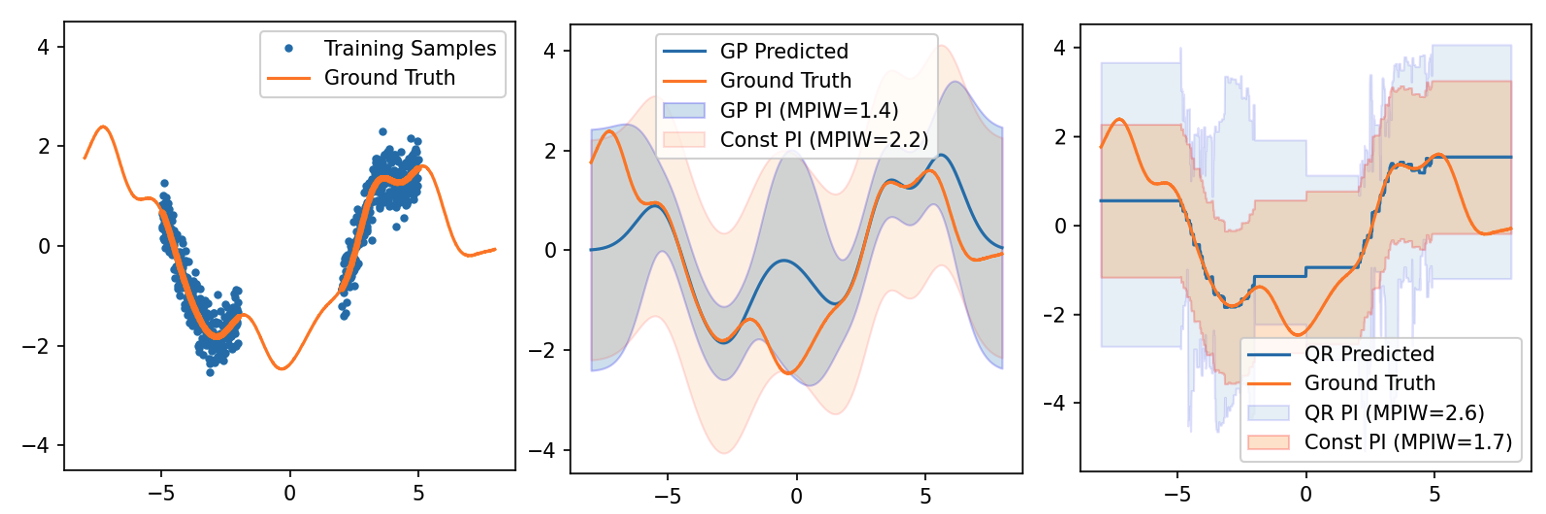
Figure 2: Example of a Gaussian Process (GP, center) and a Gradient Boosting Tree Quantile Regressor (QR, right) generating Prediction Intervals (PI) on a synthetic task (Left), along with constant-band references. All PIs are calibrated to a Miss Rate 5% and the corresponding mean bandwidth values are also shown (MPIW).

In this example, the ground truth (GT) is generated by randomly drawing from a zero-mean Gaussian Process (GP) with an RBF kernel, $f(x)\sim GP(\mathbf{0},K(x,x^{T})$. The training set is obtained as a noisy sample $y(x)\sim\mathcal{N}(f(x),0.1)$ in the regions shown in the left plot of Figure 2. Two models are fit to the data: a GP regressor (center) and a Gradient Boosted Tree (GBR) with Quantile Regression loss (QR, right). The GP and QR PIs are shown as blue-shaded areas while the light-shaded areas correspond to the reference constant bands spanned around the target predictions. All PIs are calibrated to incur a miss rate of 5%. Several observations can be made: (1) The average bandwidth (MPIW) of the GP (1.4) is lower than that of the QR (2.6). (2) The constant-band MPIW, albeit at the same miss rate, differs across the cases (2.2 for the GP vs. 1.7 for the QR). (3) The GP PI are 36% better than the reference and the QR PI are 53% worse than their reference. The last observation exercises the relative notion (gain): the GP PI are clearly superior as they capture the GT far more efficiently than the constant band. In contrast, the QR predictor generates PI that seem to be inefficient, compared to the simple reference. While the individual MPIW values are not comparable (due to the different predictors involved), we can use the relative gain to rank the quality of the PI. A method achieving a high gain is obviously valuable. A method producing zero gain may not be necessarily faulty but the task at hand may just be homoskedastic in nature, suggesting to revise our model correspondingly. Finally, negative gains indicate an inferior model.

One essential question remains open: How will the gain assessment change across different OPs (e.g. high, medium, low miss rate)? The answer lies at the foundation of the tool described next.

2.3 The Uncertainty Characteristics Curve

Scaling

In general, the goal of a calibration step is to transform the bounds such that a certain proportion of future observations, in expectation, fall within these bounds. Numerous calibration techniques have been developed in the context of regression, e.g., Kuleshov et al. (2018); Song et al. (2019). Our considerations rely on an additive-error model from which scaling emerges as fundamental: We assume the ground truth $Y$ distributes as $Y\sim F(\hat{Y},\hat{Z})$ where $F$ belongs to the location-scale family Rinne (2011), $\hat{Y}$ is an unbiased estimate of its mean, and $\hat{Z}>0$ its scale. Then

$$Y=\hat{Y}+\hat{Z}\epsilon$$ (3)

with $\epsilon\in\mathbb{R}$ a random error variable with $\epsilon\sim F(0,1)$. $\hat{Z}$ represents the (symmetric) uncertainty. A standard scale-calibration approach considers the variable $\frac{y-\hat{y}}{\hat{z}}\sim F(0,1)$ from which a desired quantile can be estimated. For instance, the quantiles $q_{0.025}$, $q_{0.975}$ can be used to obtain the prediction interval for a sample $\left[\hat{y}+\hat{z}\cdot q_{0.025},\hat{y}+\hat{z}\cdot q_{0.975}\right]$. In this model, the quantile $q$ plays a scaling role, i.e., the predicted uncertainty bound $\hat{z}$ can be scaled up or down depending on a desired expected miss rate. We adopt the scaling operation as a fundamental step behind the Uncertainty Characteristics Curve defined in the following section. Here, the location-scale (LS) assumption is a necessary limitation, however, a broad spectrum of distributions occurring in practice are genuinely LS and many others can be transformed to become LS Rinne (2011), therefore we consider this assumption mild.

The Curve

Given the scaling model above, we develop an assessment tool for prediction intervals. In this context, a single scaling value and the corresponding costs of miss rate and bandwidth, characterize a particular Operating Point (OP). A set of OPs can be obtained by varying the scale applied to ${\hat{Z}}^{l}$ and ${\hat{Z}}^{u}$ over the entire range relevant to the data $\mathbf{v}$. With $k>0$ denoting the scaling variable, we recast the dataset $\mathbf{v}$ as functions of $k$:

$$\mathbf{v}(k)=\left\{v_{i}(k)\right\}_{1\leq i\leq N}=\\ =\left\{[y_{i},\hat{y}_{i},\hat{y}_{i}-k\hat{z}_{i}^{l},\hat{y}_{i}+k\hat{z}_{i}^{u}]^{T}\right\}_{1\leq i\leq N}.$$

where $\hat{z}_{i}^{l}=\hat{y}_{i}-\hat{y}_{i}^{l}$ and $\hat{z}_{i}^{u}=\hat{y}_{i}^{u}-\hat{y}_{i}$ are the predicted bands for a sample $i$. To further simplify the notation, we use a shorthand to write the bandwidth and the miss rate as functions of $k$

$$\hat{\beta}(k):=\hat{\beta}(\mathbf{v}(k))\enspace\mbox{and}\enspace\hat{\rho}(k):=\hat{\rho}(\mathbf{v}(k)).$$ (4)

E.g., $\hat{\rho}(k)$ gives the average miss rate of the PI after re-scaling all uncertainty bands, $\hat{z}_{i}^{l,u}$ using $k$. It can be readily observed that $\hat{\beta}(k)=c\cdot k$ with $c$ a constant depending on the original dataset.

We now define the Uncertainty Characteristics Curve.

Definition 1.

The Uncertainty Characteristics Curve (UCC) is a set of operating points $\left\{\left(\hat{\beta}(k),\hat{\rho}(k)\right)\right\}_{k\in S}$ forming a bidimensional graph with the x-axis corresponding to the bandwidth and the y-axis to the miss rate, and with $S$ a set of desirable scales.

The UCC graph shows the trade-off characteristics between the two cost metrics as a function of the calibration $k$. As with the ROC Fawcett (2006), a UCC can be parametric, however, in most practical cases is considered non-parametric with the cardinality of $S$ determined by the number of observations.

An extension of the UCC to include additional axes metrics is described in the Appendix.

Given a dataset of size $N$, Algorithm 1 (see Appendix) shows an efficient computation of the UCC with a complexity of $O(N^{2})$.

figureAn illustrative example of multiple UCCs obtained for different models

figureIllustration of the Area Under Curve (AUC) and Cost within the UCC graph

An illustrative example of a UCC graph is given in Figure 2.3 showing three curves corresponding to three different models generating uncertainty bounds $\hat{z}$ around the same target predictions $\hat{y}$. Illustrative icons characterizing low, middle, and high miss rate regimes are also shown. Each UCC curve reflects the operating characteristics of its model by showing a trade-off between the two costs. In this example, the curve for model C dominates A and B and is therefore inferior as it implies higher bandwidth is needed to achieve any given miss rate. In contrast, the model A appears superior to B in a low bandwidth range, while B outperforms A in a low miss rate area. Note that each curve eventually intercepts both axes reaching a zero value.

Multiple curves on a common graph are comparable as long as the ground truth, $y$, and target predictions, $\hat{y}$, are shared across these multiple models - as is the case, for example, with a model’s PI along with with a constant-band reference. The dependence on $\hat{y}$ is due to the fact that the bounds are obtained by adding scaled bands, $kz$, to $\hat{y}$ resulting in differently shaped bounds for different $\hat{y}$ thus inducing different intersection with the observations. We give an illustrative example of this dependence in the Appendix.

Cost Function

Considering the cost trade-off between the two axes at a particular operating point, it is useful to define a function combining the two in a meaningful way. The simplest example is a linear cost function

$$C(k)=c\hat{\beta}(k)+(1-c)\hat{\rho}(k),\enspace c\in[0,1]$$ (5)

that uses an application-dependent factor, $c$, to focus on a specific area of the operating range (e.g., low miss rate area). On the UCC coordinate system, $C(k)=const$ shows as an isocost line (see Figure 2.3) whose slope is proportional to $-c/(1-c)$. A minimum achievable cost, $C(k^{*})$ with $k^{*}=\operatorname*{arg\,min}_{k}C(k)$, is an intersection of a model’s UCC and the minimal isocost as illustrated in the example. In this context, the UCC provides for a visual assessment between the original OP cost and the optimum cost as well as gives the scaling $k^{*}$ needed to reach that optimum.

In the Appendix, we point out interesting relationship between the above cost function and the well-known measures of Mean Absolute Error and Interval Score.

Area Under the UCC (AUUCC)

It is desirable to define a summary metric capturing the overall quality of a PI model. Given that the UCC coordinates correspond to costs, a sensible choice is the area under the curve (or AUUCC), as shown in Figure 2.3. Models predicting bounds that incur lower cost across the entire operating range will produce a lower AUUCC. Thus, in absence of a pre-determined operating point, the AUUCC measure can be a useful OP-agnostic indicator of the predictor’s quality. Alternatively, if a certain range of the cost, say, the miss rate values is anticipated, a partial AUUCC focusing on that range can be determined, similar to the notion of partial ROC AUC Narasimhan and Agarwal (2013).

Unlike with the ROC AUC analysis, the range of the AUUCC depends on the PI range and is therefore data dependent. This underscores the need for normalization as discussed in Section 2.2.

AUUCC Gain

We now return to the issues discussed in Section 2.2. By using the AUUCC in the relative gain calculation the question about the specific OP is integrated out, via the area calculation. Let $A_{M}$ represent the AUUCC of a model and let $A_{Const}$ refer to the constant-band counterpart. The AUUCC Gain is then defined as:

$$G_{M}=\frac{A_{Const}-A_{M}}{A_{Const}}\cdot 100\%.$$ (6)

As discussed with examples from Figure 2, negative gains are an indication of a model issue (misspecification, over-training, etc.). A positive value summarizes the overall OP-agnostic quality. The partial-AUUCC gain is calculated similarly via Eq. (6) using partial AUUCC values.

Interpreting the AUUCC

A probabilistic interpretation of the area under the ROC is well known Fawcett (2006). Bi et al. Bi and Bennett (2003) also established a connection between the area under the Regression Error Characteristics (REC) curve and the expected error. In a similar vein, we derive a probabilistic interpretation for the AUUCC.

Definition 2.

(Critical Scale). Given an observation $v_{i}=[y_{i},\hat{y}_{i},\hat{y}_{i}^{l},\hat{y}_{i}^{u}]^{T}$, a critical scale is a factor $k_{i}$ calculated according to

$$k_{i}:=\begin{cases}\frac{z_{i}}{\hat{z}_{i}^{u}}&\text{for}\,\,z_{i}\geq 0\\ -\frac{z_{i}}{\hat{z}_{i}^{l}}&\text{otherwise}\\ \end{cases}\vspace{-.2cm}$$ (7)

where $z_{i}=y_{i}-\hat{y}_{i}$, $\hat{z}_{i}^{l}=\hat{y}-\hat{y}_{i}^{l}$, and $\hat{z}_{i}^{u}=\hat{y}_{i}^{u}-\hat{y}$.

The critical value $k_{i}$ scales the active (lower or upper) error band, $\hat{z}_{i}^{l,u}$, so that it captures the observation $y_{i}$ with no excess. Note that this notion is also utilized in the Algorithm 1.

Proposition 1.

Let $B$ denote a bandwidth random variable generated by the following procedure: (i) Randomly select an observation, $v=[y,\hat{y},\hat{y}^{l},\hat{y}^{u}]^{T}$ according to $p_{V}$, (ii) determine its critical scale, $k$, via Eq. (7), and (iii) obtain the average bandwidth value via Eq. (4) using the exact metric $b={\beta}(k)$. Let $p_{B}$ denote the probability density of $B$. The area under the UCC, calculated from a finite sample $\{v_{1},...,v_{N}\}$, is an estimator of the expected value $\left<B\right>_{p_{B}}$.

The Proposition 1 states that the AUUCC estimates the expected bandwidth over the set of data-induced operating points. Consequently, for a given sample of predictions, $\{v_{1},...,v_{N}\}$, the sample average of the corresponding bandwidth values, $\{b_{1},...,b_{N}\}$, determined in Algorithm 1 approximates the AUUCC. This connection is analogous to one pointed out by Bi et al Bi and Bennett (2003) for the REC curve.

The proof of Proposition 1 along with additional results as well as more discussion can be found in the Appendix.

Significance Testing

Standard tools of significance testing are applicable to the UCC in a straight-forward manner. If a pairwise comparison between two models in terms of the AUUCC is desired, the non-parametric paired permutation test Dwass (1957) is applicable and was also used in our experiments.

3 Related Work

Uncertainty quantification in machine learning (ML) is a long-standing field of active research. Sources of uncertainty are generally categorized as epistemic or aleatoric Der Kiureghian and Ditlevsen (2009); Kendall and Gal (2017). In classification tasks, uncertainty is expressed as a measure of confidence accompanying a result Gal and Ghahramani (2016); Guo et al. (2017); Lakshminarayanan et al. (2017); Snoek et al. (2019). Combined with an optional calibration step, e.g. Zadrozny and Elkan (2002), a quality assessment of such estimates relies on summary metrics, such as the Brier score Brier and Allen (1951); Bradley et al. (2019); Lakshminarayanan et al. (2017); Guo et al. (2017); Zadrozny and Elkan (2001), Expected Calibration Error Naeini et al. (2015); Guo et al. (2017), ROC-like metrics and Accuracy-vs-Confidence curves Chen et al. (2019); Lakshminarayanan et al. (2017). Uncertainty in regression tasks involves estimating PIs (e.g., Koenker and Bassett (1978); Papoulis and Saunders (1989)) as well as in state-of-the-art ML Nix and Weigend (1994); Gal and Ghahramani (2016); Kendall and Gal (2017). However, the methodology of comparing their quality is relatively scarce, ranging from reliance on calibration and sharpness Kuleshov et al. (2018); Gneiting et al. (2007), coverage Oh et al. (2020), to using summary likelihood measures Lakshminarayanan et al. (2017).

The Uncertainty Characteristic Curve (UCC) broadens the evaluation aspect drawing an analogy to the well-known ROC Fawcett (2006). The trade-off between two costs has been studied and applied previously Gneiting et al. (2007); Dunsmore (1968); Shen et al. (2018); Tagasovska and Lopez-Paz (2019). However, most reports rely on a specific OP during the assessment stage. A connection between the cost function (Eq. (5)) and the Interval Score Gneiting et al. (2007); Dunsmore (1968) exists and is elaborated on in the Appendix. In the context of regression, Bi et al. Bi and Bennett (2003) developed an assessment tool termed Regression Error Characteristic (REC) curve utilizing a constant tolerance band around a regression target. The REC allows for a comprehensive assessment of regressors. The UCC is conceived in a similar vein. Besides the different application and metrics used, the UCC fundamentally differs from the REC by not relying on a constant tolerance band but generalizing to an arbitrary tolerance band. Finally, our work should be contrasted to calibration curves (also known as reliability diagrams) used for assessment primarily in prognostic aspects of classification tasks Niculescu-Mizil and Caruana (2005), and, more recently, in regression tasks Tran et al. (2020). A calibration curve captures the amount of over- and under-confidence in the PI with respect to observed quantiles. While these curves vary the calibration setting there are two essential differences: (1) both axes are quantiles (i.e., there is no cost trade-off relationship), and (2) the actual quality ("accuracy") of the PI is not captured. Poor PI can obtain a perfect calibration curve and vice versa.

4 Experiments

In this section we present selected case studies that highlight relevant UCC use scenarios, also referring the reader to the Appendix for an expanded report and configuration details. Result-reproducing notebooks are provided in the Supplementary Material.

UCC Implementation

The UCC was implemented in Python 3 and is available as a self-standing class providing methods to generate results shown in this paper and beyond. The UCC code along with an introductory exercise notebook is also part of the Supplementary Material, and will be made publicly available.

4.1 Synthetic Data

We begin with a basic synthetic modeling example, in which the function $x\sin x$ is mixed with an additive gaussian noise and is sampled randomly to create 5000 training points. Additionally, 1000 testing points are obtained from the non-noisy version via equidistant sampling. The training data are used to obtain a GBR target predictor using Pedregosa et al. (2011). The prediction intervals were obtained using the quantile GBR method whereby a (1) well-tuned and a (2) under-parameterized ("weak") model were created. Besides constant-band prediction intervals, we also add a random symmetric error band drawn from a uniform distribution $\hat{z}_{i}\propto U(\frac{1}{3}\sigma_{\hat{y}},3\sigma_{\hat{y}})$ with $\sigma_{\hat{y}}$ the standard deviation of $\hat{y}$, representing a "worst-case" PI. Finally, representing an ideal prediction interval, an “Epsilon-Perfect” symmetric bound was constructed as $\hat{z}_{i}=|\hat{y}_{i}-y_{i}|+\epsilon$, with $\epsilon$ being a small amount of additive noise (to visualize a curve rather than a single point). Thus, with proper scaling this bound will capture all of the observation at once, with no excess (modulo the $\epsilon$ noise), as it uses the ground truth. Figure 4.1 shows the resulting UCCs. Hollow circles mark the operating points calibrated to minimize the cost, Eq. (5), with $c=0.1$. The “$\epsilon$-perfect” curve–the best achievable curve–shows up as a vertical line reaching the x-axis at a fixed positive bandwidth (around 0.85). This is a consequence of the bandwidth metric accounting for the minimum width necessary to capture the ground truth. The remaining models rank as expected: the tuned GBR performs best, followed by the constant bound, the weak GBR, and the random bounds. A table with the full list of summary metrics can be found in the Appendix. All AUUCC values shown are significantly different at $p<0.01$, based on the pairwise permutation test Dwass (1957).

figureUCC plot with curves for the various prediction intervals on the synthetic dataset. OP stands for operating point.

figureUCC corresponding to the Gaussian Process (GP) task shown in Figure 2

figureUCC corresponding to the GBR QR model shown in Figure 2

Example from Section 2.2

Returning to the example shown in Figure 2 involving a Gaussian Process (GP) regressor and a Gradient Boosting regressor (GBR), we now plot and examine the corresponding UCCs. Figure 4.1 shows the GP and its constant-band reference. The AUUCC Gain for the GP uncertainty predictions is 57.3% indicating a good performance. From the Figure 4.1 we observe that the GP fares increasingly well as the miss rate OP decreases from 0.5 to 0.0 obtaining most of the gain. For miss rates between 0.5 and 1.0, the constant-band reference slightly outperforms the GP. Note that both curves exhibit a visible break around miss rate of 0.5. This point corresponds to a bandwidth at which both PIs fully envelope the observations inside the regions with training data availability (small prediction error) while missing most of the gap regions.

Figure 4.1 shows the UCC of the GBR portion of Figure 2. As argued in Section 2.2, the GBR model is inferior to the constant-band reference which is reflected in the UCC with the AUUCCs of 0.733 and 0.597 for the GBR and the reference, respectively. The AUUCC Gain is -31.5%.

Introductory Example from Section 1

Two BNN sampling methods, namely the Variational Inference (VI) and the Hamiltonian Monte Carlo (HMC), resulted in an inconclusive comparison in terms of log likelihood (see Figure 1). The corresponding AUUCC gains are shown in Table 1. The partial gains are calculated focusing on a miss rate range $[0,0.5]$ (i.e., high coverage).

Table 1: AUUCC Gains for the VI and the HMC methods shown in Figure 1

Method	% $G_{AUUCC}$	% $G_{Partial}$
VI	-4.3	-45.3
HMC	6.1	72.7

In spite of the VI likelihood being slightly higher than that of the HMC, the quality of the HMC bounds is nevertheless higher obtaining positive gains, which aligns with the general consensus that HMC estimates are superior Neal et al. (2011); Foong et al. (2020).

The same example offers a view of another interesting phenomenon, namely a UCC cross-over, shown in Figure 3 which zooms into the gap interval, $[-1.5,1.5]$.

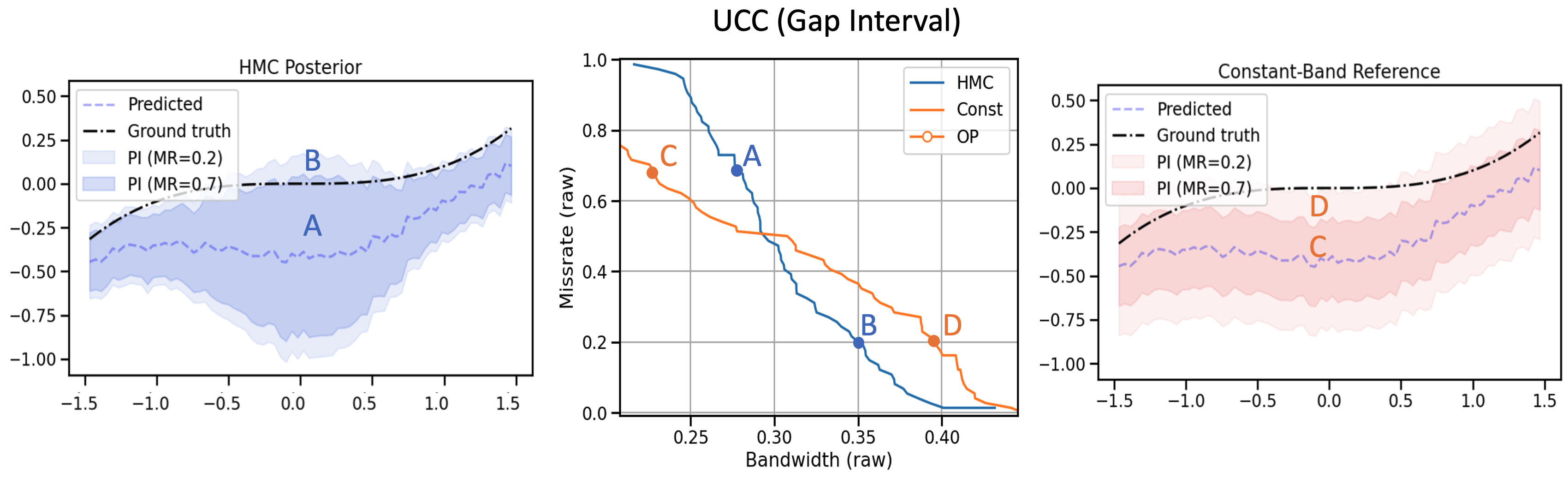
Figure 3: Zoomed section of the gap interval from Figure 1 with UCC cross-over. MR stands for Miss Rate.

The chart highlights two distinct OPs for each curve. OPs A and C lie in a high miss rate range. In this regime, as shown in the data plot on the left, both PI miss 70% of the observations, however, the HMC’s bandwidth is higher (its center-widened PI are closer to but have not reached the observations in the center). Therefore the HMC UCC lies above the reference UCC. The situation is reversed for OPs B and D which operate at miss rates of 0.2. At this miss rate, the HMC’s central-gap widening becomes beneficial and captures the observations without excessive bandwidth, unlike the constant band, as shown on the left-hand side of the figure.

The above cross-over phenomenon underscores the power of insight in the UCC: Evaluating the above PIs at any fixed operating point would tell an incomplete story, the conclusion of which depends on the operating point chosen.

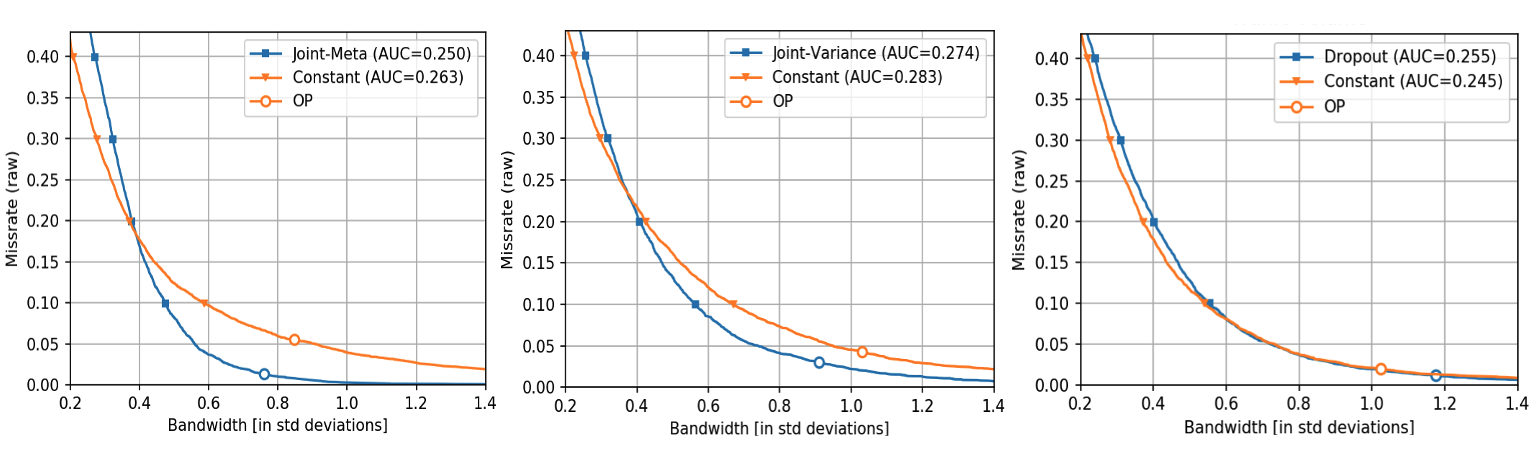
Figure 4: UCCs obtained on the Traffic dataset using an LSTM-based target predictor and three different techniques

4.2 Real-World Datasets

We chose three real-world datasets, namely (1) the Boston Housing Dataset, (2) the Wine Quality Dataset Cortez et al. (2009), and (3) Metro Interstate Traffic Volume.

For brevity we only present results of the Traffic dataset in the main paper referring the reader to the Appendix for a comprehensive set of UCC results.

For the sequential Traffic Volume task we employed an LSTM-based sequence-to-sequence architecture developed in Authors (2020). In this study, several approaches of generating prediction intervals were taken: (1) “Joint Meta” (JMS) model with an internal component learning to generate symmetric prediction intervals. The JMS component has a recursive structure trained jointly with the target predictor; (2) “Joint-Variance” model (JMV) - a similar sequence-to-sequence model with additional output nodes implicitly modeling the heteroskedastic variance via a gaussian likelihood loss, similar to Lakshminarayanan et al. (2017); Kendall and Gal (2017); Oh et al. (2020); (3) Variational Dropout (DOMS) - a model with an LSTM structure trained according to Gal and Ghahramani (2016) to generate multiple output sequences. While the mean of the multiple outputs serves as the target predictor, their variance determines the (symmetric) prediction intervals. Note that all three cases represent time-varying, symmetric prediction intervals. Figure 4 shows the three UCCs. It can be observed that while the JMS and JMV models outperform their constant baselines in the low miss rate range (< 0.2), the DOMS case performs comparably to the constant for most of the range. The overall AUUCC gains are as follows: 4.9% (JMS), 3.2% (JMV), and -4.0% (DOMS).

"Cross-overs" can be seen in all cases, underscoring the need for a systematic visualization the UCC offers.

It may be argued that certain UCC ranges may not be of practical interest, for example, miss rates of 50% or more may be considered too high. We believe that, as an OP-agnostic tool, the UCC should include the full range in absence of a-priori knowledge. It is conceivable that certain applications may be tuned to “reject” (miss) 50% or more observations if their inclusion is associated with a high cost (e.g. accepting a potential anomaly as normal). The argument may only be fully resolved by having a concrete set of applications at hand. Then the UCC analysis can be adapted by focusing on partial AUUCC as discussed above.

5 Conclusions

In this work we introduced the Uncertainty Characteristics Curve (UCC) in conjunction with a gain metric relative to constant-band references, and demonstrated its power in diagnostics of prediction intervals. The UCC is formed by varying a scaling-based calibration applied to the prediction intervals, thus characterizing their quality in an operating point agnostic manner. We analyzed the area under the curve and tied its value to certain probabilistic expectations of the metrics involved. In several experimental case studies, the UCC was shown to provide important insights in terms of both the AUUCC gain metrics and the operating characteristics along the calibration range. With the release of the corresponding code, we believe the UCC will become a valuable new addition in the diagnostic toolbox for ML researchers and practitioners alike.

6 Acknowledgements

We thank Karthikeyan Shanmugam of IBM Research and David Klusáček of the Faculty of Mathematics and Physics of the Charles University in Prague for helpful discussions regarding the proofs in this manuscript.

Appendix to Paper: Uncertainty Characteristics Curves: A Systematic Assessment of Prediction Intervals

7 Algorithm to calculate the UCC

Algorithm 1 Algorithm to calculate the UCC

Input: Ground truth, predictions, uncertainty estimates $\{y_{i},\hat{y}_{i},\hat{y}_{i}^{l},\hat{y}_{i}^{u}\}_{1\leq i\leq N}$

Output: Set of UCC points $\{x_{i},y_{i}\}_{1\leq i\leq N}$

for $i\leftarrow 1$ to $N$ do

     $z_{i}\leftarrow y_{i}-\hat{y}_{i}$ $\triangleright$ Observed error

     $k_{i}\leftarrow\begin{cases}\frac{z_{i}}{\hat{y}_{i}^{u}-\hat{y}}&\text{for}\,\,z_{i}\geq 0\\ -\frac{z_{i}}{\hat{y}-\hat{y}_{i}^{l}}&\text{otherwise}\\ \end{cases}$ $\triangleright$ Critical scale

     $x_{i}\leftarrow\hat{\beta}(k_{i})$ $\triangleright$ $\hat{\beta},\hat{\rho}$ defined in Eq. (4)

     $y_{i}\leftarrow\hat{\rho}(k_{i})$

end for

8 Confounding predictions and uncertainty: An example

Suppose there is a model predicting the regression target, $\hat{y}$, as well as a gaussian uncertainty with mean $\hat{y}$ and variance $\hat{\sigma}^{2}$. The loss with respect to model parameters $\theta$ is a function of both the predictions, $\hat{y}_{i}$ and the uncertainties, $\hat{\sigma}_{i}$: $-logP(\theta)=\frac{1}{2}\sum_{i}^{N}\frac{(y_{i}-\hat{y}_{i})^{2}}{\hat{\sigma}_{i}^{2}}+\log\hat{\sigma}_{i}^{2}+C$. We refer to the fact that the loss combines these two predictive aspects (target and uncertainty) as "comfounding" in the main paper.

9 Additional Metrics

In addition to bandwidth and miss rate, defined in Section 2.1, we define two additional, related metrics as follows

Excess:

$$\qquad\xi(V) =\operatorname{\mathbb{E}}\left[\mathbf{1}_{Y\in[\hat{Y}^{l},\hat{Y}^{u}]}\cdot\min\left\{Y-\hat{Y}^{l},\hat{Y}^{u}-Y\right\}\right]$$

$$\qquad\hat{\xi}(\mathbf{v}) =\frac{1}{N}\sum_{i:y_{i}\in[\hat{y}_{i}^{l},\hat{y}_{i}^{u}]}\min\left\{y_{i}-\hat{y}_{i}^{l},\hat{y}_{i}^{u}-y_{i}\right\}$$ (8)

Deficit:

$$\qquad\delta(V) =\operatorname{\mathbb{E}}_{p_{V}}\left[\mathbf{1}_{Y\notin[\hat{Y}^{l},\hat{Y}^{u}]}\cdot\min\left\{\left|Y-\hat{Y}^{l}\right|,\left|Y-\hat{Y}^{u}\right|\right\}\right]$$

$$\qquad\hat{\delta}(\mathbf{v}) =\frac{1}{N}\sum_{i:y_{i}\notin[\hat{y}_{i}^{l},\hat{y}_{i}^{u}]}\min\left\{|y_{i}-\hat{y}_{i}^{l}|,|y_{i}-\hat{y}_{i}^{u}|\right\}$$ (9)

Figure 5 illustrates all four metrics. The relative proportion of observations lying outside the bounds (i.e., the miss rate) ignores the extent of the bounds’ shortfall. The proposed Deficit, Eq. (9), captures this aspect. The type 2 cost is captured by the Bandwidth, Eq. (2). However, its range is indirectly compounded by the underlying variation in ${\hat{Y}}$ and ${Y}$. Therefore we propose the Excess measure, Eq. (8), which also reflects the Type 2 cost, but just the portion above the minimum bandwidth necessary to include the observation.

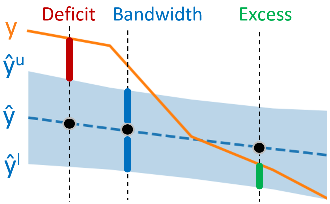
Figure 5: Bandwidth, excess, and deficit costs.

We will be using Excess and Deficit in reporting additional results in this document and also present an additional theoretical result for a UCC on Excess-Deficit coordinates.

10 Illustration of the effect of $\hat{y}$ on the UCC

In Section 2.3 we mention that multiple curves can be plotted in a common UCC chart only if they are obtained using same observations, $y$, and target predictions, $\hat{y}$. A simple example of two PI is shown in Figure 6. Both PI are constant bands, i.e., they should be characterized by an identical UCC. However, because they relate each to different target predictions, $\hat{y_{1}}$ and $\hat{y_{2}}$, their behavior with respect to the observation, $y$, is completely different. While the PI of $\hat{y_{1}}$ captures the observation fully at a certain critical scale leading to a "perfect" curve (UCC1), the PI of $\hat{y_{2}}$ incurs a positive miss rate even at the same bandwidth. As the bandwidth varies the characteristics of the curved PI intersecting the observation will be non-trivial leading to a "rounder" curve (UCC2) as illustrated.

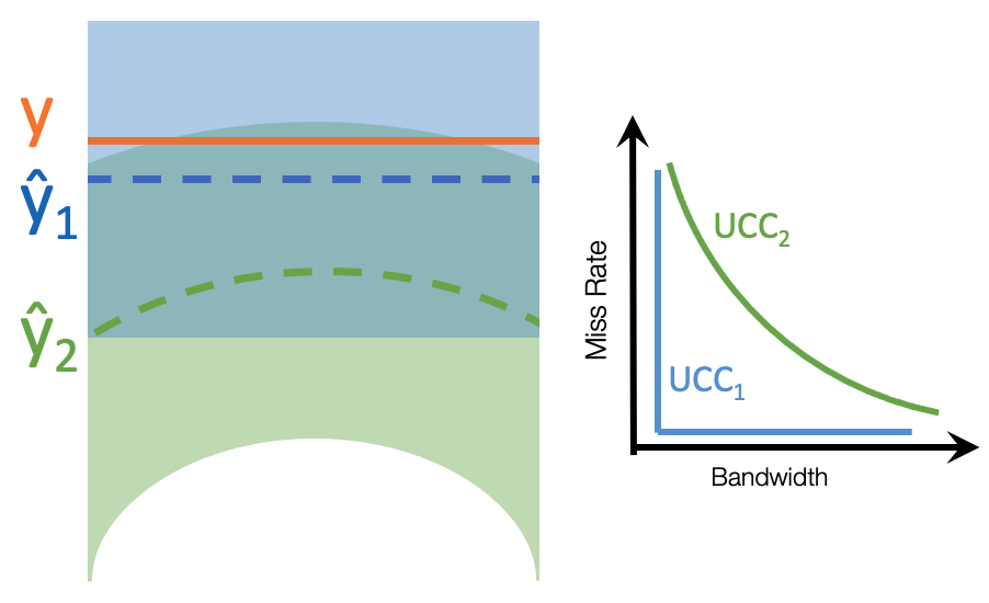
Figure 6: Illustrative example of how identical PI–constant bands in both cases–lead to different UCCs if they relate to different target predictions, $\hat{y}$

This also highlights the need for normalization which is achieved by calculating the AUUCC gain (see Eq. (6)) which, in the same example, would result in a gain of 0% for both cases thus making the PI equivalent in terms of their quality.

11 Proofs And Additional Results

To prove Proposition 1 we use the Definition 2 and the Lemma 1 below:

Lemma 1.

Choose any $v_{i}\in\mathbf{v}$, with $\mathbf{v}$ a sample set as defined in Section 2.1. Let $k_{i}$ be the critical scale for $v_{i}$ and $K$ the scale random variable. The following holds

$$P(Y\notin[\hat{Y}-k_{i}\hat{Z}^{l},\hat{Y}+k_{i}\hat{Z}^{u}])\equiv 1-P(K\leq k_{i}).$$

Proof.

Let $\{k_{1},...,k_{N}\}$ be the set of critical scales corresponding to $\{v_{1},...,v_{N}\}$ and let $k_{1}^{\prime}\leq...\leq k_{N}^{\prime}$ denote a sorted sequence of such scales. By definition of the critical scale, for any $k_{i}^{\prime}$ in the sequence there are exactly $i$ samples falling within, and $N-i$ falling outside their bounds scaled by $k_{i}$, i.e.,

$$y_{j}\in[\hat{y}_{j}-k_{i}\hat{z}_{j}^{l},\hat{y}_{j}+k_{i}\hat{z}_{j}^{u}]\qquad\forall j:k_{j}^{\prime}\leq k_{i}^{\prime}$$

$$y_{j}\notin[\hat{y}_{j}-k_{i}\hat{z}_{j}^{l},\hat{y}_{j}+k_{i}\hat{z}_{j}^{u}]\qquad\forall j:k_{j}^{\prime}>k_{i}^{\prime}$$

(Note that in the case of ties only the element with highest index $i$ among the tie set is considered.) Thus, the fraction $\frac{N-i}{N}$ corresponds to the empirical miss rate as a function of $k$ (see Eq. (4)), which is an estimator of the miss rate probability $P(Y\notin[\hat{Y}-k_{i}\hat{Z}^{l},\hat{Y}+k_{i}\hat{Z}^{u}])$. On the other hand, considering $K$ a critical scale of a randomly drawn sample, $V$, the fraction $\frac{i}{N}$ is an estimator for the cumulative distribution function $P_{K}(k_{i}):=P(K\leq k_{i})$. Hence

$$1-P_{K}(k_{i})\equiv P(Y\notin[\hat{Y}-k_{i}\hat{Z}^{l},\hat{Y}+k_{i}\hat{Z}^{u}]).$$

∎

11.1 Proof of Proposition 1

Remark 1.

The bandwidth $\hat{\beta}$ and excess $\hat{\xi}$ (Eq. (4)) are monotonically increasing functions of the scale $k$.

Proof.

Using the fact that $B\geq 0$, its expected value can be written as follows:

$$\left<B\right>_{p}=\int_{0}^{\infty}bp_{B}(b)db=\int_{0}^{\infty}[1-P_{B}(b)]db$$ (10)

where $P_{B}$ denotes the cumulative distribution function of $B$. The second equality uses the tail expectation formula Casella and Berger [2001].

Since $1-P_{B}(b)=P(B>b)$ and $\beta$ is a monotonic function of $k$ it holds that

$$P(K>k)\equiv P(B>b).$$ (11)

From the above and the Lemma 1, it follows that $P(B>b)$ corresponds to the miss rate associated with the bandwidth $b=\beta(k)$:

$$P_{m}(b):=P(Y\notin[\hat{Y}-k\hat{Z}^{l},\hat{Y}+k\hat{Z}^{u}])\equiv 1-P_{B}(b)$$ (12)

Hence, Eq. (10) becomes

$$\left<B\right>_{p_{B}}=\int_{0}^{\infty}P_{m}(b)db.$$ (13)

Given $N$ samples, $\mathbf{v}=\{v_{1},...,v_{N}\}$ from $p_{V}$, we calculate the set of critical values, $\{k_{1},...,k_{N}\}$. The sorted sequence, $k_{1}^{\prime}\leq k_{2}^{\prime}\leq...\leq k_{N}^{\prime}$ gives rise to a sequence of bandwidths $b_{1}\leq...\leq b_{N}$. The Riemann sum corresponding to the integral (13) is as follows

$$S(N)=\sum_{i=1}^{N}P_{m}(b_{i}^{\prime})\Delta b_{i}$$ (14)

with a partitioning determined by the sorted observations, $b_{1}\leq...\leq b_{N}$, $\Delta b_{i}=b_{i}-b_{i-1}$, $b_{0}=0$, and $b_{i}^{\prime}\in[b_{i-1},b_{i}]$. Choosing $b_{i}^{\prime}=b_{i}$ we rewrite the sum (14) as

$$S(N)=\sum_{i=1}^{N}\hat{\rho}(k_{i}^{\prime})[b(k_{i}^{\prime})-b(k_{i-1}^{\prime})]$$ (15)

with $\hat{\rho}$ being the empirical miss rate, as per Eq. (4).

Eq. (15) corresponds to evaluating the area under the UCC using the rectangular rule. The sum will approach the expected bandwidth value in Eq. (10) as $\lim_{N\rightarrow\infty}S(N)$. Thus, the empirical AUUCC is an estimator for the expected bandwidth when using bandwidth-miss rate coordinates.

∎

According to Proposition 1, given a dataset, and given the miss rate being one of the coordinates, the AUUCC amounts to the other metric’s average over the entire operating range. A smaller AUUCC relates to smaller average bandwidth (or excess) measurements as the calibration scale $k$ varies, as expected from prediction intervals of higher quality.

Corollary 1.

The area under the UCC with excess-miss rate coordinates is an estimator of the expected value $\left<X\right>_{p_{X}}$ with $X$ the excess random variable and $p_{X}$ its density function.

The proof of Corollary 1 follows trivially from the proof of Proposition 1 by replacing the bandwidth variable, $B$, with excess, $X$.

11.2 AUUCC on the Excess-Deficit Coordinates2

Proposition 2.

Let $X$ and $D$ be the excess and deficit random variables generated by randomly selecting a sample, $v$, determining its critical scale, $k$, and obtaining their values via Eq. (4). Let the UCC be defined on the excess-deficit coordinates, $(\hat{\xi},\hat{\delta})$, and the metrics $\rho,\xi,\delta$ be differentiable and invertible functions. The area under the UCC is an estimator of a quantity proportional to the expected value $\left<D\right>_{q}$ with respect to a density given by $q(d)=\frac{p_{D}(d)}{p_{X}(\delta^{-1}(d))}/Q$, where $p_{D}$, $p_{X}$ denote deficit and excess densities and $Q$ is a normalizing constant, $Q=\int_{0}^{\infty}\frac{p_{D}(d)}{p_{X}(\delta^{-1}(d))}dd$.

In this case, the interpretation involves an expectation of the deficit metric proportional to a density ratio of the deficit and the excess.

Proof.

Let the excess variable, $x=X$, be associated with the abscissa, and $\delta(x)$ be the deficit function of the excess on the ordinate axis. The AUUCC is

$$\int_{0}^{\infty}\delta(x)dx.$$ (16)

Now consider the UCC a parametric curve parametrized by the miss rate, $r\in[0,1]$. Let $r=\rho_{X}(x)$ and $r=\rho_{D}(d)$ where $\rho_{X,D}$ denotes a miss rate function of the excess and deficit, respectively. Then $x=\rho_{X}^{-1}(r)$ and $d=\rho_{D}^{-1}(r)$, and Eq. (16) can be rewritten as

$$\int_{1}^{0}\delta(\rho_{X}^{-1}(r))[\rho_{X}^{-1}]^{\prime}(r)dr$$ (17)

It is easy to show that $\frac{d}{dr}\left[\rho_{X}^{-1}(r)\right]=-\frac{1}{p_{X}(x)}$, where $p_{X}>0$ refers to the excess density. Hence (17) becomes

$$\int_{0}^{1}\delta(\rho_{X}^{-1}(r))\frac{1}{p_{X}(\rho_{X}^{-1}(r))}dr.$$ (18)

After applying a variable change $r=\rho_{D}(d)$, Eq. (18) becomes

$$\int_{0}^{\infty}d\cdot\frac{p_{D}(d)}{p_{X}(\delta^{-1}(d))}dd$$ (19)

where $p_{D}$ refers to the deficit density. We normalize the density ratio in Eq. (19) to obtain

$$AUC=Q\cdot\int_{0}^{\infty}d\cdot q(d)dd\enspace\propto\left<D\right>_{q}$$ (20)

whereby $q(d):=\frac{p_{D}(d)}{p_{X}(\delta^{-1}(d))}/Q$ and $Q=\int_{0}^{\infty}\frac{p_{D}(d)}{p_{X}(\delta^{-1}(d))}dd$. Thus, the Eq. (20) shows the AUUCC is proportional to the expected deficit with respect to the distribution, $q$. Using the Riemann sum argument, similar to one in the proof to Proposition 1, it is straight-forward to show that the empirical AUUCC is an estimator for (20) up to the constant $Q$. ∎

In the case of Proposition 2, the interpretation involves again an expectation of one of the axes’ metrics, namely the deficit, however, with respect to a distribution of a density ratio between the deficit and the excess. Similar to the previous result, a smaller AUUCC relates to a smaller deficit average with respect to the density, $q$. One example of such average being small would be a case where the mode of $p_{D}$ lies near zero deficit and the corresponding $p_{X}$ is small there, with its mode residing at higher deficits, thus concentrating the mass of $q$ around small deficit values.

Exploiting these results in the optimization of models to produce better prediction intervals appears an interesting avenue for future work.

11.3 Special Cases of the Linear Cost Function

Remark 2.

Let $d_{i}=|\hat{y}_{i}-y_{i}|$. Given a scale $k$, and symmetric prediction bands $\hat{z}_{i}:=\hat{z}_{i}^{l}=\hat{z}_{i}^{u}$, the linear cost (5) with $c=0.5$ at any operating point $k$ on the excess-deficit coordinate system corresponds to half of the mean absolute error (MAE) between the absolute difference and the scaled band: $MAE(k)=\frac{1}{N}\sum_{i}|d_{i}-k\cdot z_{i}|$.

Remark 3.

For the choice of $f_{1}=\hat{\beta},f_{2}=\hat{\delta}$ and $c=\frac{1}{\alpha+1}$ with $\alpha\in[0,1]$ denoting the confidence level, the symmetric cost (5) corresponds to the well-known Interval Score (see Gneiting et al. [2007], Section 6.2), up to a scale $\frac{\alpha+1}{\alpha}$.

12 Model Configurations

The Gradient Boosting Regressors (GBR) used in Sections 4.1 and 4.2 were trained with hyperparameter values listed in Table 2. No tuning was performed as we adopted the values from URL [2021]. The "GBR-Weak" was set up by reducing the tree depth to 3, and the number of trees (estimators) to 50.

The LSTM configuration details are listed in the Appendix of Authors [2020] - a pdf version of which is included in the Supplementary Material.

In addition, notebooks with code to reproduce all UCC results shown in Section 4.1, 4.2, and this Appendix, are also included in the Supplementary Material.

Table 2: GBR hyperparameter settings as used to produce results in Section 4.1 and 4.2

. Hyper- Where Value parameter used Num. of estimators GBR 500 Max. tree depth GBR 10 Subsample fraction both 0.7 Num. of estimators GBR-Weak 50 Max. tree depth GBR-Weak 3 Random seed both 42 Learning rate both 0.1 Min. samples per leaf both 9

BNN Setup for the Introductory Example

We used a BNN with a single hidden layer, ReLU activations, and a hundred hidden units. Synthetic data details: Targets are generated as $y=0.1x^{3}+\epsilon$, where $\epsilon\sim\mathcal{N}(0,0.25)$. Evaluated on 70 training inputs uniformly sampled from $[-3.1,-1]\cup[1,3.1]$ and 154 test inputs uniformly sampled from $[-3.1,3.1]$. Variational inference (VI): We used doubly reparameterized variational inference with the local reparameterization trick Kingma et al. [2015]. We used twenty MonteCarlo samples for computing the stochastic gradients of the evidence lower bound (ELBO). We used five random-restarts and selected the solution with the highest ELBO. Hamiltonian Monte Carlo (HMC): We used HMC with the leapfrog integrator. We sampled the momentum variable from $\mathcal{N}(0,\mathbf{I})$, and used $L=100$ leapfrog steps. We used 50K iterations and a burnin of 40K and a thinning of interval twenty following the settings described in previous work Yao et al. [2019]. We used a fixed step size of $5\times 10^{-4}$. Test log likelihood evaluation: For both HMC and VI we used $500$ samples from the respective approximations to evaluate the test log-likelihood. Test log-likelihood is defined as:

$$\mathbb{E}_{(x_{n},y_{n})\sim D}[\mathbb{E}_{q(W)}[p(y_{n}\mid x_{n},W)]]$$

13 Additional Experimental Results

13.1 Synthetic Data

The data used to produce the results in Section 4.1 are generated using a function $x\sin x$. The training data is created by sampling this function and adding a gaussian noise with randomly varying variance, as in URL [2021]. We set the range to be $x\in[0,20]$. A total of 4000 training samples were used to create the GBR models, and 1000 equidistant, non-noisy samples sweeping the entire range of $x$ were used for evaluation. Additional 1000 held-out set samples were generated for tuning the operating points. The synthetic data and the GBR model predictions are shown in Figure 7. The ground truth in the plot is the function $x\sin x$. A subset of the noisy training samples, the GBR target predictions, and the GBR prediction intervals are shown. The prediction intervals are tuned to contain, on average, 95% of the ground truth.

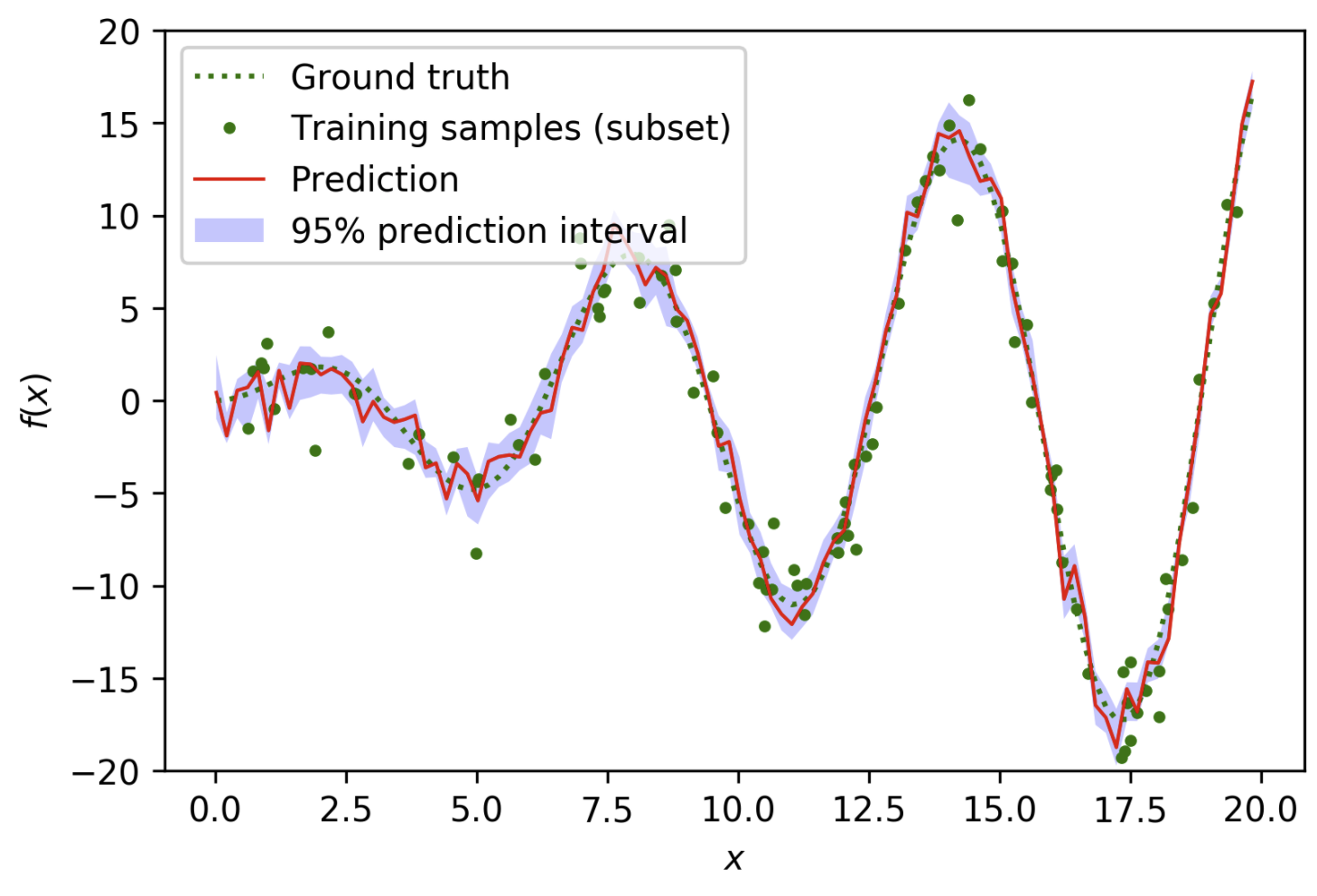
Figure 7: The synthetic dataset: a function $x\sin x$ is sampled and added noise producing training samples. The latter are used to train the GBR target and bound predictors. Also shown is the ground truth (the function $x\sin x$ without the noise), the target prediction as well as the prediction intervals. The ground truth is expected to lie within the bound about 95% of the time.

Table 3: Summary metrics obtained on the synthetic dataset

Model	Excess-Deficit			Bandwidth-Miss rate
	AUUCC	Cost	Opt. Cost	AUUCC	Cost	Opt. Cost	MAE
GBR	0.138	0.308	0.099	0.645	0.318	0.178	0.750
Constant	0.209	0.287	0.136	0.819	0.371	0.245	0.960
GBR-Weak	0.311	0.377	0.182	0.939	0.405	0.292	1.284
Random	0.412	0.329	0.208	1.108	0.425	0.333	1.128
Eps-Perfect	0.001	0.002	0.002	0.779	0.109	0.085	0.022

The resulting UCCs are shown in the Figure 4.1 in Section 4.1 of the main paper. Here, summary metrics for the same experiment are shown in Table 3. These include the AUUCC, the Cost, the Optimum Cost, and the Mean Absolute Error (MAE). While the Cost is calculated at the operating point (OP) determined on the held-out dataset, the Minimum Cost is calculated on the test data themselves, thus representing a minimum achievable cost. The MAE is defined in the Remark in Section 2. All values in Table 3 are consistent with the overall model ranking apparent in the Figure 4.1. The rather large gap between the actual and minimum cost can be attributed to the fact that the held-out data set contains noise, while the test set does not. This gap disappears when using a held-out set without noise.

13.2 Real-World Datasets

Figure 8 shows the UCCs on excess-deficit (left) and bandwidth-miss rate (right) coordinates. Note that here we apply axes normalization to standard deviation units. Comparing the predictors across the two coordinate systems reveals interesting differences. While there is a clear separation of all the curves on the bandwidth-miss rate plot, the gap narrows for all but the weak GBR. For example, at one standard deviation of bandwidth there is a 5% difference in miss rate between the GBR and the Weak GBR predictor - a difference comparable to one between GBR and the Meta predictor. However, when the extent of missing a target is taken into account (in the Excess-Deficit plot), the Weak GBR fares significantly worse than the GBR by same comparison, indicating the Weak GBR tends to miss targets by a greater extent.

Figure 8: The UCCs on excess-deficit (left) and bandwidth-miss rate (right) coordinates for the Boston Housing data set.

Furthermore, a curve cross-over can be seen for the GBR and the Meta model on the excess-deficit plot, comparable to that observed on the Wine dataset (see below). This pattern is not present on the bandwidth-miss rate coordinate system - an indication that the choice of metrics is not without consequences and should be made carefully with the eventual application in mind.

13.3 Wine Quality Data

We used the White Wine portion of the collection (comprising White and Red), consisting of 4897 samples. Furthermore, to obtain more robust results, we applied a 5-fold cross-validation scheme to generate our measurements.

The UCC for both the excess-deficit and the bandwidth-miss rate coordinates are shown in Figure 9. Interestingly, there are a few significant differences between the two plots: while the Meta model performs best in both coordinate systems, the GBR model falls behind the constant when bandwidth and miss rate are measured. Recall that the miss rate is insensitive to the extent of prediction interval excess, while the excess metric captures this. Furthermore, the GBR-Weak model shows a dramatic drop at a bandwidth of about 1.3 standard deviations. A further investigation revealed that the weak GBR model’s predictions are almost constant (with a few exceptions). This combined with the fact that the wine ratings are whole numbers between 1 and 10, but mostly concentrating between 5 and 7 (mode at 6), there is a distinct OP that just captures a large portion of the ground truth ratings at once. This becomes visible as a jump in the UCC when miss rate is one of the coordinates.

The summary metrics are shown in Table 4. Significantly smaller gaps can be seen between the Cost and the Opt. Cost, as compared to the synthetic data (as discussed above). While most summary metrics reflect the model ranking consistently, one outlier is the optimum cost for the GBR-Weak model on the bandwidth-miss rate coordinate system: based on this metric the GBR-Weak model might be considered the superior choice. A look at the corresponding UCCs (Figure 9), however, is revealing: the GBR-Weak model exhibit a dramatic drop in miss rate around the bandwidth of 1.3, to the degree that it briefly dips below all other curves, thus bringing the minimum achievable cost to 0.187. However, from the UCC comparison it is clear that such a choice may not be the most robust one.

Figure 9: The UCCs on excess-deficit (left) and bandwidth-miss rate (right) coordinates for the Wine Quality dataset.

Table 4: Summary metrics obtained on the Wine Quality dataset

Model	Excess-Deficit			Bandwidth-Miss rate
	AUUCC	Cost	Opt. Cost	AUUCC	Cost	Opt. Cost	MAE
GBR	0.139	0.119	0.115	0.500	0.199	0.198	1.031
Constant	0.143	0.128	0.119	0.485	0.199	0.197	1.082
GBR-Weak	0.167	0.126	0.125	0.545	0.187	0.187	1.074
Meta	0.136	0.132	0.115	0.478	0.196	0.193	1.294

13.4 Boston Housing Data

Due to the relatively small size of the Housing dataset, the following complexity-related parameters of the GBR and GBR-Weak models were adjusted (compared to values listed in the Table 2): (1) number of estimators (trees) set to 50 and 10 for GBR and GBR-Weak, respectively, (2) maximum tree depth set to 3. A 10-fold cross-validation (with 2 randomized repetitions) was applied to obtain more reliable measurements.

The summary metrics are shown in Table 5.

Table 5: Summary metrics obtained on the Boston Housing data set

Model	Excess-Deficit			Bandwidth-Miss rate
	AUUCC	Cost	Opt. Cost	AUUCC	Cost	Opt. Cost	MAE
GBR	0.039	0.078	0.061	0.394	0.169	0.162	104.762
Constant	0.036	0.080	0.059	0.250	0.113	0.108	45.962
GBR-Weak	0.073	0.103	0.080	0.527	0.200	0.196	112.331
Meta	0.037	0.102	0.061	0.298	0.143	0.133	113.851

13.5 Traffic Volume Data

The full set of UCCs using both coordinate systems is shown in Figure 10.

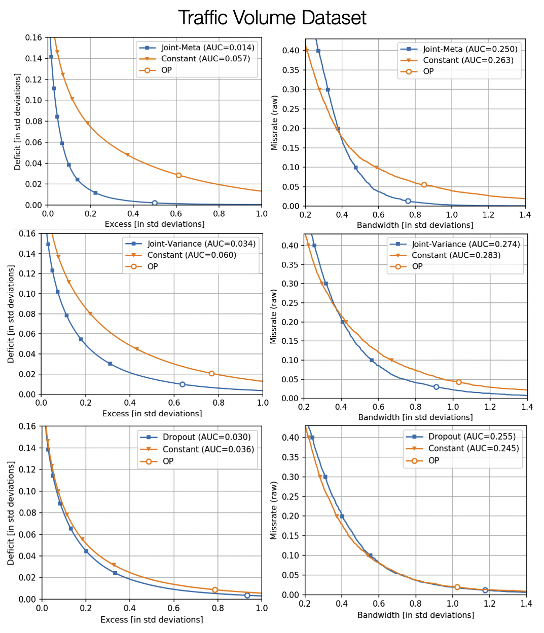
Figure 10: The UCCs on excess-deficit (left) and bandwidth-miss rate (right) coordinates for the three models (Joint-Meta, Joint-Variance, Dropout) and their respective constant baselines.

The findings from Figure 10 are also reflected in the gains (see Table 6) with the JMS achieving an overall improvement of 75.5% and 59.3% in AUUCC ($G_{AUC}$) and optimum cost ($G_{C^{*}}$) over its constant reference. In contrast, the DOMS model obtains rel. smaller positive gains for AUUCC and the minimum cost, but negative gains for the original-calibration cost ($G_{C}$) and the MAE, indicating the original calibration present in the input data was suboptimal. Recall that while $G_{C}$ and $G_{MAE}$ are determined using the original calibration, which is tuned to minimize the cost using a held-out set of training data, the gain $G_{C^{*}}$ is determined on the best calibration achievable using the visualized data. The AUUCC values in each graph are significantly different at $p<0.01$ based on the pairwise permutation test.

Table 6: The sequential Traffic Volume task. Summary metrics shown as percentage gains over the corresponding constant-band baselines.

Model	Excess-Deficit
	% $G_{AUC}$	% $G_{C}$	% $G_{C^{*}}$	% $G_{MAE}$
JMS	75.5	40.5	59.3	21.8
JMV	42.7	24.1	30.4	18.2
DOMS	15.5	-11.5	10.0	-17.8

In addition to the discussion in Section 4.2, we observe that an interesting cross-over pattern occurs in the bandwidth-miss rate UCC plots showing the constant band outperforming the relatively complex sequential models (Joint-Meta and Joint-Variance) in a high miss rate operating range. As the operating miss rate gets lower (below 0.2), the model-based prediction intervals begin gaining over the constant baseline significantly. This pattern does not show up on the excess-deficit plots and seems to be induced, again, by the miss rate metrics ignoring the degree of excess, as discussed earlier.

References

- Arnold et al. (2019) M. Arnold, R. K. E. Bellamy, M. Hind, S. Houde, S. Mehta, A. Mojsilović, R. Nair, K. N. Ramamurthy, A. Olteanu, D. Piorkowski, D. Reimer, J. Richards, J. Tsay, and K. R. Varshney. Factsheets: Increasing trust in ai services through supplier’s declarations of conformity. IBM Journal of Research and Development, 63(4/5):6:1–6:13, July 2019. ISSN 0018-8646. doi: 10.1147/JRD.2019.2942288.
- Authors (2020) A. Authors. Anonymized. In Anonymized copy included in the Supplementary Material. To appear in arXiv;. arxiv, 2020.
- Begoli et al. (2019) E. Begoli, T. Bhattacharya, and D. Kusnezov. The need for uncertainty quantification in machine-assisted medical decision making. Nature Mach Intell, 1:20–23, 2019.
- Bi and Bennett (2003) J. Bi and K. P. Bennett. Regression error characteristic curves. In Proceedings of the Twentieth International Conference on International Conference on Machine Learning, ICML’03, page 43–50. AAAI Press, 2003. ISBN 1577351894.
- Bradley et al. (2019) A. A. Bradley, J. Demargne, and K. J. Franz. Attributes of Forecast Quality, pages 849–892. Springer Berlin Heidelberg, Berlin, Heidelberg, 2019. ISBN 978-3-642-39925-1. doi: 10.1007/978-3-642-39925-1_2. URL https://doi.org/10.1007/978-3-642-39925-1_2.
- Brier and Allen (1951) G. W. Brier and R. A. Allen. Verification of Weather Forecasts, pages 841–848. American Meteorological Society, Boston, MA, 1951. ISBN 978-1-940033-70-9. doi: 10.1007/978-1-940033-70-9_68. URL https://doi.org/10.1007/978-1-940033-70-9_68.
- Casella and Berger (2001) G. Casella and R. Berger. Statistical Inference. Duxbury Resource Center, June 2001. ISBN 0534243126.
- Chen et al. (2019) T. Chen, J. Navrátil, V. Iyengar, and K. Shanmugam. Confidence scoring using whitebox meta-models with linear classifier probes. In The 22nd International Conference on Artificial Intelligence and Statistics, AISTATS 2019, 16-18 April 2019, Naha, Okinawa, Japan, pages 1467–1475, 2019.
- Cortez et al. (2009) P. Cortez, A. Cerdeira, F. Almeida, T. Matos, and J. Reis. Modeling wine preferences by data mining from physicochemical properties. Decis. Support Syst., 47(4):547–553, Nov. 2009. ISSN 0167-9236. doi: 10.1016/j.dss.2009.05.016. URL https://doi.org/10.1016/j.dss.2009.05.016.
- Der Kiureghian and Ditlevsen (2009) A. Der Kiureghian and O. Ditlevsen. Aleatoric or epistemic? does it matter? Structural Safety, 31(2):105–112, 2009. ISSN 0167-4730. doi: 10.1016/j.strusafe.2008.06.020.
- Dunsmore (1968) I. R. Dunsmore. A bayesian approach to calibration. Journal of the Royal Statistical Society: Series B (Methodological), 30(2):396–405, 1968. doi: 10.1111/j.2517-6161.1968.tb00740.x. URL https://rss.onlinelibrary.wiley.com/doi/abs/10.1111/j.2517-6161.1968.tb00740.x.
- Dwass (1957) M. Dwass. Modified randomization tests for nonparametric hypotheses. Ann. Math. Statist., 28(1):181–187, 03 1957. doi: 10.1214/aoms/1177707045.
- Fawcett (2006) T. Fawcett. An introduction to roc analysis. Pattern Recognition Letters, 27(8):861 – 874, 2006. ISSN 0167-8655. doi: https://doi.org/10.1016/j.patrec.2005.10.010. URL http://www.sciencedirect.com/science/article/pii/S016786550500303X. ROC Analysis in Pattern Recognition.
- Foong et al. (2020) A. Foong, D. Burt, Y. Li, and R. Turner. On the expressiveness of approximate inference in bayesian neural networks. In H. Larochelle, M. Ranzato, R. Hadsell, M. F. Balcan, and H. Lin, editors, Advances in Neural Information Processing Systems, volume 33, pages 15897–15908. Curran Associates, Inc., 2020.
- Gal and Ghahramani (2016) Y. Gal and Z. Ghahramani. A theoretically grounded application of dropout in recurrent neural networks. In D. D. Lee, M. Sugiyama, U. V. Luxburg, I. Guyon, and R. Garnett, editors, Advances in Neural Information Processing Systems 29, pages 1019–1027. Curran Associates, Inc., 2016.
- Gneiting et al. (2007) T. Gneiting, F. Balabdaoui, and A. E. Raftery. Probabilistic forecasts, calibration and sharpness. Journal of the Royal Statistical Society: Series B (Statistical Methodology), 69(2):243–268, 2007. doi: 10.1111/j.1467-9868.2007.00587.x. URL https://rss.onlinelibrary.wiley.com/doi/abs/10.1111/j.1467-9868.2007.00587.x.
- Guo et al. (2017) C. Guo, G. Pleiss, Y. Sun, and K. Q. Weinberger. On calibration of modern neural networks. In Proceedings of the 34th International Conference on Machine Learning - Volume 70, ICML’17, page 1321–1330. JMLR.org, 2017.
- Jiang et al. (2018) H. Jiang, B. Kim, M. Guan, and M. Gupta. To trust or not to trust a classifier. In S. Bengio, H. Wallach, H. Larochelle, K. Grauman, N. Cesa-Bianchi, and R. Garnett, editors, Advances in Neural Information Processing Systems 31, pages 5541–5552. Curran Associates, Inc., 2018.
- Kendall and Gal (2017) A. Kendall and Y. Gal. What uncertainties do we need in bayesian deep learning for computer vision? In I. Guyon, U. V. Luxburg, S. Bengio, H. Wallach, R. Fergus, S. Vishwanathan, and R. Garnett, editors, Advances in Neural Information Processing Systems 30, pages 5574–5584. Curran Associates, Inc., 2017.
- Kingma et al. (2015) D. P. Kingma, T. Salimans, and M. Welling. Variational dropout and the local reparameterization trick. arXiv preprint arXiv:1506.02557, 2015.
- Koenker and Bassett (1978) R. W. Koenker and G. Bassett. Regression quantiles. Econometrica, 46(1):33–50, 1978. URL https://EconPapers.repec.org/RePEc:ecm:emetrp:v:46:y:1978:i:1:p:33-50.
- Kuleshov et al. (2018) V. Kuleshov, N. Fenner, and S. Ermon. Accurate uncertainties for deep learning using calibrated regression. In J. Dy and A. Krause, editors, Proceedings of the 35th International Conference on Machine Learning, volume 80 of Proceedings of Machine Learning Research, pages 2796–2804, Stockholmsmässan, Stockholm Sweden, 10–15 Jul 2018. PMLR. URL http://proceedings.mlr.press/v80/kuleshov18a.html.
- Lakshminarayanan et al. (2017) B. Lakshminarayanan, A. Pritzel, and C. Blundell. Simple and scalable predictive uncertainty estimation using deep ensembles. In I. Guyon, U. V. Luxburg, S. Bengio, H. Wallach, R. Fergus, S. Vishwanathan, and R. Garnett, editors, Advances in Neural Information Processing Systems 30, pages 6402–6413. Curran Associates, Inc., 2017.
- Naeini et al. (2015) M. P. Naeini, G. F. Cooper, and M. Hauskrecht. Obtaining well calibrated probabilities using bayesian binning. In Proceedings of the Twenty-Ninth AAAI Conference on Artificial Intelligence, AAAI’15, page 2901–2907. AAAI Press, 2015. ISBN 0262511290.
- Narasimhan and Agarwal (2013) H. Narasimhan and S. Agarwal. A structural SVM based approach for optimizing partial auc. In S. Dasgupta and D. McAllester, editors, Proceedings of Machine Learning Research, volume 28, pages 516–524, Atlanta, Georgia, USA, 17–19 Jun 2013. PMLR. URL http://proceedings.mlr.press/v28/narasimhan13.html.
- Neal et al. (2011) R. M. Neal et al. Mcmc using hamiltonian dynamics. Handbook of markov chain monte carlo, 2(11):2, 2011.
- Niculescu-Mizil and Caruana (2005) A. Niculescu-Mizil and R. Caruana. Predicting good probabilities with supervised learning. In Proceedings of the 22nd International Conference on Machine Learning, ICML ’05, page 625–632, New York, NY, USA, 2005. Association for Computing Machinery. ISBN 1595931805. doi: 10.1145/1102351.1102430. URL https://doi.org/10.1145/1102351.1102430.
- Nix and Weigend (1994) D. A. Nix and A. S. Weigend. Estimating the mean and variance of the target probability distribution. In Proceedings of 1994 IEEE International Conference on Neural Networks (ICNN’94), volume 1, pages 55–60 vol.1, June 1994. doi: 10.1109/ICNN.1994.374138.
- Oh et al. (2020) M. Oh, P. A. Olsen, and K. N. Ramamurthy. Crowd counting with decomposed uncertainty. In AAAI Conference on Artificial Intelligence, 2020.
- Papoulis and Saunders (1989) A. Papoulis and H. Saunders. Probability, Random Variables and Stochastic Processes (2nd Edition). Journal of Vibration, Acoustics, Stress, and Reliability in Design, 111(1):123–125, 01 1989. ISSN 0739-3717. doi: 10.1115/1.3269815.
- Pedregosa et al. (2011) F. Pedregosa, G. Varoquaux, A. Gramfort, V. Michel, B. Thirion, O. Grisel, M. Blondel, P. Prettenhofer, R. Weiss, V. Dubourg, J. Vanderplas, A. Passos, D. Cournapeau, M. Brucher, M. Perrot, and E. Duchesnay. Scikit-learn: Machine learning in Python. Journal of Machine Learning Research, 12:2825–2830, 2011.
- Rinne (2011) H. Rinne. Location-Scale Distributions, pages 752–754. Springer Berlin Heidelberg, Berlin, Heidelberg, 2011. ISBN 978-3-642-04898-2. doi: 10.1007/978-3-642-04898-2_341. URL https://doi.org/10.1007/978-3-642-04898-2_341.
- Shen et al. (2018) Y. Shen, X. Wang, and J. Chen. Wind power forecasting using multi-objective evolutionary algorithms for wavelet neural network-optimized prediction intervals. Applied Sciences, 8(2):185, Jan 2018. ISSN 2076-3417. doi: 10.3390/app8020185.
- Snoek et al. (2019) J. Snoek, Y. Ovadia, E. Fertig, B. Lakshminarayanan, S. Nowozin, D. Sculley, J. Dillon, J. Ren, and Z. Nado. Can you trust your model’s uncertainty? evaluating predictive uncertainty under dataset shift. In Advances in Neural Information Processing Systems, pages 13969–13980, 2019.
- Song et al. (2019) H. Song, T. Diethe, M. Kull, and P. Flach. Distribution calibration for regression. In K. Chaudhuri and R. Salakhutdinov, editors, International Conference on Machine Learning, 9-15 June 2019, Long Beach, California, USA, Proceedings of Machine Learning Research, pages 5897–5906. Proceedings of Machine Learning Research, May 2019.
- Steel and Torrie (1960) R. G. D. Steel and J. H. Torrie. Principles and procedures of statistics. McGraw-Hill Book Company, Inc., New York, Toronto, London, 1960.
- Tagasovska and Lopez-Paz (2019) N. Tagasovska and D. Lopez-Paz. Single-model uncertainties for deep learning. In H. Wallach, H. Larochelle, A. Beygelzimer, F. d’ Alché-Buc, E. Fox, and R. Garnett, editors, Advances in Neural Information Processing Systems 32, pages 6417–6428. Curran Associates, Inc., 2019. URL http://papers.nips.cc/paper/8870-single-model-uncertainties-for-deep-learning.pdf.
- Tran et al. (2020) K. Tran, W. Neiswanger, J. Yoon, Q. Zhang, E. Xing, and Z. W. Ulissi. Methods for comparing uncertainty quantifications for material property predictions. Machine Learning: Science and Technology, 1(2):025006, 2020.
- URL (2021) . URL. Prediction intervals for gradient boosting regression. https://scikit-learn.org/stable/auto_examples/ensemble/plot_gradient_boosting_quantile.html, 2021.
- Yao et al. (2019) J. Yao, W. Pan, S. Ghosh, and F. Doshi-Velez. Quality of uncertainty quantification for bayesian neural network inference. ICML workshop on uncertainty in deep learning, 2019.
- Zadrozny and Elkan (2001) B. Zadrozny and C. Elkan. Obtaining calibrated probability estimates from decision trees and naive bayesian classifiers. In In Proceedings of the Eighteenth International Conference on Machine Learning, pages 609–616. Morgan Kaufmann, 2001.
- Zadrozny and Elkan (2002) B. Zadrozny and C. Elkan. Transforming classifier scores into accurate multiclass probability estimates. In Proceedings of the Eighth ACM SIGKDD International Conference on Knowledge Discovery and Data Mining, KDD ’02, pages 694–699, New York, NY, USA, 2002. ACM. ISBN 1-58113-567-X.