Entanglement Classification via Single Entanglement Measure

Abstract

We provide necessary and sufficient conditions for generic n-qubit states to be equivalent under Stochastic Local Operations with Classical Communication (SLOCC) using a single polynomial entanglement measure. SLOCC operations may be represented geometrically by Möbius transformations on the roots of the entanglement measure on the Bloch sphere. Moreover, we show how the roots of the 3-tangle measure classify 4-qubit generic states, and propose a method to obtain the normal form of a 4-qubit state which bypasses the possibly infinite iterative procedure.

Quantum entanglement is one of the key manifestations of quantum mechanics and the main resource for technologies founded on quantum information science. In particular, quantum states with non-equivalent entanglement represent distinct resources which may be useful for different protocols. The idea of clustering states into classes exhibiting different qualities under quantum information processing tasks resulted in their classification under stochastic local operations assisted by classical communication (SLOCC). Such a classification was successfully presented for two, three and four qubits Dür et al. (2000); Verstraete et al. (2001); Gour and Wallach (2013); Li et al. (2009). However, the full classification of larger systems is completely unkown. Even the much simpler problem of detecting if two $n$-qubit states ($n>4$) are SLOCC-equivalent is, in general, quite demanding Viehmann et al. (2011); Zhang et al. (2016); Gour and Wallach (2011); Burchardt and Raissi (2020).

Among several approaches to the entanglement quantification and classification problem, a particularly useful one is via SL-invariant polynomial (SLIP) measures. Well-known examples are concurrence and $3$-tangle, which measure the 2-body and 3-body quantum correlations of the system Wootters (1998); Coffman et al. (2000a). SLIP measures provide not only a convenient method for entanglement classification but also its practical detection. Indeed, it was shown that almost all SLOCC equivalence classes can be distinguished by ratios of such measures Gour and Wallach (2013). Any given two n-qubit states are then SLOCC-equivalent if a complete set of SLIP measures has the same values for both of them Viehmann et al. (2011). For more than four qubits, however, the size of such a set grows exponentially, making it intractable to use this approach to discriminate SLOCC-equivalent states with more than four qubits Love et al. (2007).

In this Letter, we show that a single SLIP measure is enough to provide necessary and sufficient conditions for any two generic pure n-qubit states to be SLOCC-equivalent, by looking at how the roots of the SLIP measure for those states behave under SLOCC. In essence, if the states are SLOCC-equivalent, then the roots of the SLIP measure for each state must be related by a Möbius transformation, which is straightforward to verify. We use this procedure to show how the 3-tangle measure is enough to discriminate between generic 4-qubit states. Finally, we show how one may use the roots of a SLIP entanglement measure to obtain the normal form of a 4-qubit state which bypasses the possibly infinite iterative standard procedure.

Polynomial Invariant Measures—An entanglement measure is a function $E(\ket{\psi})$ defined for pure states of $n$ qubits which vanishes on the set of separable states. One of the desired features of entanglement measures is invariance under SLOCC operations. Mathematically, a SLOCC operation might be uniquely determined by the action of local invertible operators $L\in\text{SL(}2,\mathbb{C}\text{)}^{\otimes n}$ Dür et al. (2000). An entanglement measure $E(\ket{\psi})$ defined on the system of $n$ qubits is called a SL-invariant polynomial of homogeneous degree $h$ if it is polynomial in the coefficients of a pure state $\ket{\psi}$ and satisfies

$$E\big{(}\kappa L\ket{\psi}\big{)}=\kappa^{h}E\big{(}\ket{\psi}\big{)}$$ (1)

for each real constant $\kappa>0$ and invertible linear operator $L$ Dür et al. (2000); Gour and Wallach (2013); Eltschka and Siewert (2014). We denote such a measure as $\text{SLIP}_{n}^{h}$, where the upper index indicates the degree of the polynomial and the lower index is related to the number of qubits.

Any SLIP measure $E$ can also be extended to mixed states by determining the largest convex function on the set of mixed states which coincides with $E$ on the set of pure states Uhlmann (1998). Despite its simple definition, the evaluation of a convex roof extension requires non-linear minimization procedure, and for a general density matrix is a challenging task Tóth et al. (2015); Osborne and Verstraete (2006); Regula et al. (2014, 2016). An attempt to address this challenging task was carried out by introducing the so-called zero-polytope, the convex hull of pure states with vanishing $E$ measure Osterloh et al. (2008); Lohmayer et al. (2006); Osterloh (2016); Gartzke and Osterloh (2018). In the particular case of rank-2 density matrices $\rho$, the zero-polytope can be represented inside a Bloch sphere, spanned by the roots of $E$ Lohmayer et al. (2006); Regula and Adesso (2016a). We adapt this approach focusing only on the roots of polynomial invariants, equivalently the vertices of the zero-polytope.

System of roots—Consider a $(n+1)$-partite qubit state $\ket{\psi}$. The state $\ket{\psi}$ can be uniquelly written as

$$\ket{\psi}=\ket{0}\ket{\psi_{0}}+\ket{1}\ket{\psi_{1}}\,,$$ (2)

providing the canonical decomposition of the reduced density matrix $\rho=\ket{\psi_{0}}\bra{\psi_{0}}+\ket{\psi_{1}}\bra{\psi_{1}}$ obtained by tracing out the first qubit. Note that the states $\ket{\psi_{0}}$ and $\ket{\psi_{1}}$ are in general neither normalized nor orthogonal. Consider now the family of states

$$\ket{\psi_{z}}=z\ket{\psi_{0}}+\ket{\psi_{1}},$$ (3)

where $z$ is taken from the extended complex plane $\hat{\mathbb{C}}$, i.e., complex numbers plus infinity. We denote this the extended plane representation. In addition, consider any $\text{SLIP}_{n}^{h}$ measure $E$ defined on the set of $n$-partite pure qubit states. Since $E$ is polynomial in the coefficients of $\ket{\psi_{z}}$, it is also polynomial in the complex variable $z$ Osterloh et al. (2008). Therefore, the polynomial $E(z\ket{\psi_{0}}+\ket{\psi_{1}})$ has exactly $h$ roots: $\zeta_{1},\ldots,\zeta_{h}$ (which may be degenerated and/or at infinity), related to the degree of $E$. By using the complex number $z$, the states $\ket{\psi_{z}}$ can be mapped to the surface of a sphere via the standard stereographic projection $(\theta,\phi):=(\text{arctan}\,1/|z|,\;-\text{arg}\,z)$ written in spherical coordinates. This way, a point on the unit 2-sphere $(\theta,\phi)$ can be associated with the quantum state

$$\ket{\widetilde{\psi}_{z}}:=\text{cos}\dfrac{\theta}{2}\ket{\psi_{0}}+\text{sin}\dfrac{\theta}{2}e^{i\phi}\ket{\psi_{1}}$$ (4)

with $z=\text{ctg}({\theta}/{2})\>e^{-i\phi}$, such that $\ket{\psi_{0}}$ lies in the North pole and $\ket{\psi_{1}}$ lies in the South pole, see Figure 1. We denote this the Bloch sphere representation. Note that ${\ket{\widetilde{\psi}_{z}}\propto\ket{\psi_{z}}}$ and that neither of these states is normalized, since $\ket{\psi_{0}}$ and $\ket{\psi_{1}}$ are not normalized in general either.

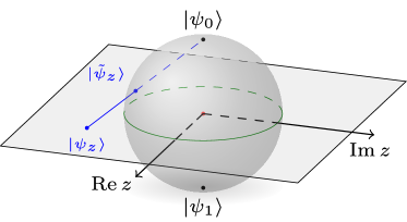
Figure 1: The stereographic projection relating the family of states $\ket{\psi_{z}}$ on the extended complex plane with the associated family of states $\ket{\widetilde{\psi_{z}}}$ on the Bloch sphere. The spherical coordinates $({\theta},\phi)$ and the complex coordinate $z$ are related via the stereographic projection $z=\text{ctg}({\theta}/{2})\>e^{-i\phi}$.

Local operations on the system of roots—To each linear invertible operator $\mathcal{O}=\begin{pmatrix}a&b\\ c&d\end{pmatrix}$, one may associate a Möbius transformation $z\mapsto z^{\prime}:=\frac{az+b}{cz+d}$, mapping the extended complex plane $\hat{\mathbb{C}}$ into itself Bengtsson and Zyczkowski (2017); Aulbach (2012). The composition of such transformations represents the multiplication of the associated operators. In particular, $z\mapsto z^{\prime}:=\frac{dz-b}{-cz+a}$ is an inverse Möbius transformation related with $\mathcal{O}^{-1}=\begin{pmatrix}d&-b\\ -c&a\end{pmatrix}$. Note that although Möbius transformations are typically represented on the extended complex plane, one may represent them as transformations on the Bloch sphere via the stereographic projection. The correspondence between invertible operators and Möbius transformations represented on the Bloch sphere was already successfully used for SLOCC classification of permutation-symmetric states Bastin et al. (2009); Ribeiro and Mosseri (2011); Kam and Liu (2020).

To study the effect of SLOCC operations on the system of roots we begin by acting on the first qubit of a state $\ket{\psi}$ written in the form of Eq. (2) with an invertible linear operator $\mathcal{O}$. In terms of the family of states $\ket{\psi_{z}}$ in Eq. (3), this operation induces the map

$$\ket{\psi_{z}}\mapsto\ket{\psi_{z^{\prime}}}=\frac{az+b}{cz+d}\ket{\psi_{0}}+\ket{\psi_{1}}\,,$$ (5)

i.e. the index is mapped via the Möbius transformation $z\mapsto z^{\prime}:=\frac{az+b}{cz+d}$ (see Supplementary Material Section 1). In addition, since ${\ket{\widetilde{\psi}_{z}}\propto\ket{\psi_{z}}}$, we have that the family of states $\ket{\widetilde{\psi}_{z}}$ also transforms according to Eq. (5). This reflects the fact that the states $\ket{\psi_{z}}$ and $\ket{\widetilde{\psi}_{z}}$ associated to the extended complex plane and the Bloch sphere are related by a stereographic projection of the variable $z$. Using Eq. (5) and the defining equation $E(\zeta_{i}\ket{\psi_{0}}+\ket{\psi_{1}})=0$ for the roots $\zeta_{i}$ of the polynomial $E$, one concludes that the roots transform according to the inverse Möbius transformation associated to the operator $\mathcal{O}$, i.e. $\zeta_{i}\mapsto\frac{d\zeta_{i}-b}{-c\zeta_{i}+a}$. Finally, although the system of roots changes with local operations acting on the qubit that is being traced out in Eq. (2), it is invariant under local operations acting on any other qubit since the polynomial $E$ is $\text{SL(}2,\mathbb{C}\text{)}^{\otimes n}$ invariant. We summarize these results in the theorem below (see Supplementary Material Section 1 for a detailed proof).

Theorem 1.

Consider an $(n+1)$-partite pure quantum state $\ket{\psi}=\ket{0}\ket{\psi_{0}}+\ket{1}\ket{\psi_{1}}$. The roots $\zeta_{i}$ of any $\text{SLIP}_{n}^{h}$ entanglement measure associated to the partial trace of the first qubit:

1. are invariant under invertible operators, i.e. invariant under $\textbf{1}\otimes\mathcal{O}_{\vec{n}}\in\text{SL(}2,\mathbb{C}\text{)}^{\otimes n}$ operators;

2. transform via an inverse Möbius transformation $\zeta_{i}^{\prime}=\frac{d\zeta_{i}-b}{-c\zeta_{i}+a}$ w.r.t the $\mathcal{O}=\begin{pmatrix}a&b\\ c&d\end{pmatrix}\otimes\textbf{1}^{n}$ operator.

It is crucial to emphasize that normalizing the states $\ket{\psi_{0}}$ and $\ket{\psi_{1}}$ after the action of the operator $\mathcal{O}$, as is the case in existing related works Osterloh et al. (2008); Lohmayer et al. (2006); Gartzke and Osterloh (2018); Regula and Adesso (2016a, b), would spoil the mapping of Eq. 5. As a consequence, the action of SLOCC operators on the states $\ket{\psi_{z}}$ would no longer be given by the corresponding Möbius transformation, and the statements in Theorem 1 would no longer hold.

State discrimination—The decomposition (2) can be performed with respect to any other subsystem, each with its own system of roots. This is particularly important for entanglement classification schemes where the presence of entanglement after partial trace is an aspect of focus, such as in Quinta and André (2018); Quinta et al. (2019). Any local operator $\mathcal{O}_{k}=\begin{pmatrix}a&b\\ c&d\end{pmatrix}$ acting on the $k$-th qubit will influence independently the corresponding $k$-th system of roots and its associated zero-polytope via the Möbius transformation $\zeta_{i}\mapsto\frac{d\zeta_{i}-b}{-c\zeta_{i}+a}$. On the other hand, if acting globally with a local operator $\mathcal{O}_{1}\otimes\cdots\otimes\mathcal{O}_{n+1}$, all roots (and thus all zero-polytopes) will be affected. Since a Möbius transformation is a bijective mapping on the Bloch sphere, the total number of roots will always be preserved Regula and Adesso (2016b). Moreover, the existence of a local transformation between two given states becomes straightforward to verify since Möbius transformations are fully classified.

This way, Theorem 1 provides a solution for the problem of discriminating $(n+1)$-qubit states up to SLOCC-equivalence Viehmann et al. (2011); Zhang et al. (2016); Gour and Wallach (2011); Burchardt and Raissi (2020). Indeed, Möbius transformation associated with the SLOCC operation transforms a system of roots of polynomial invariants of a given state onto a system of roots of an equivalent state. To verify if two pure states are SLOCC-equivalent, one can thus use the following procedure:

• Choose any $\text{SLIP}_{n}^{h}$ entanglement measure of degree $h\geq 3$ and calculate its roots for each subsystem for both states (note that a generic state will always have $h$ roots for each subsystem);

• Focus on one subsystem $i$, $1\leq i\leq n+1$ and choose 3 of the $h$ roots from each state;

• Write the unique Möbius transformations between the two triplets of roots and derive the local operator $\mathcal{O}_{i}$ associated to it;

• Choose a different set of 3 out of the h roots of the second state and repeat step 3). Do this for all $3!{{h}\choose{3}}$ possibilities;

• Repeat steps 3) and 4) for all other subsystems and then consider the tensor products of all the local operators obtained, resulting in a finite set of operators of the form $\mathcal{O}_{1}\otimes\dots\otimes\mathcal{O}_{n+1}$;

• If the two given $(n+1)$-qubit states are SLOCC-equivalent, one of these operators must transform one state into the other. Otherwise, they are not SLOCC-equivalent.

The above procedure has two main important features. Firstly, it factorizes the problem of finding SLOCC-equivalence, i.e. local operations are determined separately for each subsystem. Secondly, it discretizes the initial discrimination task since there are at most $(3!{{h}\choose{3}})^{n+1}$ local operators which might provide SLOCC equivalence between initial states.

State classification–Any three distinct points on the sphere can be transformed onto any other three distinct points via a unique Möbius transformation. While this is not the case for four points, it is possible to take any four complex points $z_{1},z_{2},z_{3},z_{4}$ and associate a so-called cross-ratio

$$\lambda\big{(}z_{1},z_{2},z_{3},z_{4}\big{)}:=\dfrac{z_{3}-z_{1}}{z_{3}-z_{2}}\dfrac{z_{4}-z_{2}}{z_{4}-z_{1}}\,,$$ (6)

which is preserved under Möbius transformations Ribeiro and Mosseri (2011); Bengtsson and Zyczkowski (2017). Systems of four distinct points are related via Möbius transformations if their cross-ratios are related in the same way. The cross-ratio is not invariant under permutations of points, however, and depending on the ordering taken for the four points, it takes six values: $\lambda,\frac{1}{\lambda},1-\lambda,\frac{1}{1-\lambda},\frac{\lambda-1}{\lambda},\frac{\lambda}{\lambda-1}$ Ribeiro and Mosseri (2011). A particular interesting set of four points is one of the form $z,1/z,-z,-1/z$, which we call a normal system. Any set of four points may be mapped into a normal system, for which $z,1/z,-z,-1/z$ will be the solutions of the fourth degree equation $\lambda=4z^{2}/(1+z^{2})^{2}$, where $\lambda$ is the corresponding cross-ratio from Eq. (6). Such a map is unique up to symmetries of the cube, i.e the group of $24$ rotations generated by $\pi/2$ rotations along the $X,Y,Z$ axis, denoted by $\mathcal{G}_{24}$.

It is particularly straightforward how one may use the normal system of roots for SLOCC-classification of small dimensional systems. Focusing first on the three-qubit case, genuinely entangled pure states are SLOCC-equivalent to either $\ket{\textrm{GHZ}}=\frac{1}{\sqrt{2}}(\ket{000}+\ket{111})$ or $\ket{\textrm{W}}=\frac{1}{\sqrt{3}}(\ket{001}+\ket{010}+\ket{100})$ Sudbery (2001). Using the 2-tangle $\tau^{(2)}$ Wootters (1998) as the entanglement measure, one may use the roots to distinguish between the two classes. Indeed, all rank-2 reduced density matrices of the $\ket{\textrm{W}}$ state have a single root, while there are always two distinct roots for the $\ket{\textrm{GHZ}}$ state Regula and Adesso (2016a).

Contrary to the three qubit case, there are infinitely many SLOCC classes of four qubit states Sudbery (2001). Although four qubit states were divided into nine families Verstraete et al. (2001); Oleg Chterental (2007); Spee et al. (2016), we will focus on generic 4-qubit states, i.e. 4-qubit states with random coefficients belonging to the so called $G_{abcd}$ family - the 4-qubit SLOCC family with the most degrees of freedom. The representative state is of the form $\ket{G_{abcd}}=\frac{a+d}{2}\big{(}\ket{0000}+\ket{1111}\big{)}+\frac{a-d}{2}\big{(}\ket{0011}+\ket{1100}\big{)}+\frac{b+c}{2}\big{(}\ket{0101}+\ket{1010}\big{)}+\frac{b-c}{2}\big{(}\ket{0110}+\ket{1001}\big{)}$, where $a^{2}\neq b^{2}\neq c^{2}\neq d^{2}$ are pairwise different. Choosing the 3-tangle $\tau^{(3)}$ Coffman et al. (2000b) as the entanglement measure, the states $\ket{G_{abcd}}$ have four non-degenerate roots already in the normal form (see Supplementary Material Section 3). Since the normal form of roots is unique up to the group $\mathcal{G}_{24}$, the problem of SLOCC-equivalence of states $\ket{G_{abcd}}$ becomes solvable, with a discrete amount of solutions. Indeed, it can quickly be confirmed if two states in the $G_{abcd}$ class are SLOCC equivalent by checking if one can be obtained from the other by the action of an element of the finite class of operators $\mathcal{O}\in\mathcal{G}_{24}^{\otimes 4}$. We thus find that exactly 192 states of the form $\ket{G_{abcd}}$ are SLOCC-equivalent.

Proposition 1.

Two states $\ket{G_{abcd}}$ and $\ket{G_{a^{\prime}b^{\prime}c^{\prime}d^{\prime}}}$ are SLOCC-equivalent iff their coefficients are related by the following three operations: multiplication by a phase factor $(a^{\prime},b^{\prime},c^{\prime},d^{\prime})=e^{i\phi}(a,b,c,d)$, and permutation of coefficients $(a^{\prime},b^{\prime},c^{\prime},d^{\prime})=\sigma(a,b,c,d)$, and change of sign in front of two coefficients from $a,b,c,d$.

See Supplementary Material Section 3 for a more detailed analysis. The symmetry in Proposition 1 is given by the Weyl group of Cartan type $D_{4}$ and it has already been observed that the generators of four-qubit polynomial invariants exhibit this type of symmetry Luque and Thibon (2003); Oleg Chterental (2007). As a consequence, this result constitutes a new relation between 4-qubit invariants and the convex roof extension of 3-tangle $\tau^{(3)}$, which may shed some light on the problem of generalizing the CKW inequality Coffman et al. (2000a) for four qubit states Gour and Wallach (2010); Eltschka et al. (2009); Regula et al. (2014); Eltschka and Siewert (2014); Regula et al. (2016), and beyond Eltschka et al. (2009); Gour and Wallach (2010); Eltschka and Siewert (2015).

Finally, we remark a link between normal systems of roots and the normal form of pure states of four qubits belonging to the $G_{abcd}$ class. A state is in its normal form if its reductions are maximally mixed Verstraete et al. (2003). Although the process to determine the normal form of a state (if it exists) is straightforward, it may also turn out to be an infinite iterative process Verstraete et al. (2003). However, the results of Theorem 1 applied to the four qubits states of the $G_{abcd}$ class show that this difficulty can be avoided. Indeed, the representative state of the $G_{abcd}$ family is in normal form Verstraete et al. (2003) and its corresponding roots associated with the $\tau^{(3)}$ measure also form a normal system. Thus, one may calculate the roots associated with any state in the $G_{abcd}$ class, quickly transform them into a normal system of roots using a Möbius transformation and use the associated SLOCC operator to convert the initial state into a state in the normal form. We illustrate this procedure by transforming the widely discussed four-partite state $\frac{1}{\sqrt{2}}(\ket{0}\ket{\textrm{GHZ}}+\ket{1}\ket{\textrm{W}})$ Gartzke and Osterloh (2018); Lohmayer et al. (2006) into its normal form, see Figure 2. Without this technique, the standard way of obtaining the normal form would indeed result in an infinite iterative procedure.

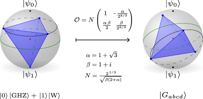
Figure 2: The system of four roots (represented as blue dots) related to the 3-tangle polynomial measure $\tau^{(3)}$ evaluated on the first subsystem of the state $1/\sqrt{2}(\ket{0}\ket{\textrm{GHZ}}+\ket{1}\ket{\textrm{W}})$. This system of four points can be mapped into a normal system (i.e. symmetrically related points $z,-z,1/z,-1/z$) by a Möbius transformation. Similar local transformations can be performed with respect to other subsystems, transforming the states into a state in the normal form.

Conclusions—In this letter, we showed how a single $\text{SLIP}_{n}^{h}$ entanglement measure can be used to derive necessary and sufficient conditions for any two $(n+1)$-qubit states to be SLOCC equivalent. This was possible by showing that the roots of any $\text{SLIP}_{n}^{h}$ measure transform via Möbius transformations under the SLOCC operations performed on the subsystems. In that way, SLOCC equivalence between two states is implied by the easily verifiable existence of a Möbius transformation relating aforementioned roots for each subsystem. We demonstrated our approach on 4-qubit states, and showed that the roots of the 3-tangle measure $\tau^{(3)}$ are enough to classify 4-qubit states from the most generic $G_{abcd}$ family. Lastly, a procedure was presented to determine the normal form of states in the $G_{abcd}$ family that circumvents the possibility of an infinite iterative process of the standard procedure.

Acknowledgements— The authors thank Andreas Osterloh, Karol Życzkowski, Rui Perdigão and Yasser Omar for fruitful discussions. A.B acknowledges support from the National Science Center under grant number DEC-2015/18/A ST2/00274. G.Q. thanks the support from Fundação para a Ciência e a Tecnologia (Portugal), namely through projects CEECIND/02474/2018 and project UIDB/50008/2020 and IT project QuantSat-PT. R.A. acknowledges support from the Doctoral Programme in the Physics and Mathematics of Information (DP-PMI) and the Fundação para a Ciência e Tecnologia (FCT) through Grant No. PD/BD/135011/2017.

Supplemental Material for
“Entanglement Classification via Single Entanglement Measure”

I Section 1. Proof of Theorem 1

We present a proof for Theorem 1. Any $n+1$ partite qubit state $\ket{\psi}\in\mathcal{H}_{2}^{\otimes(n+1)}$ might be written as

$$\ket{\psi}=\ket{0}\ket{\psi_{0}}+\ket{1}\ket{\psi_{1}}.$$ (S1)

Such a form provides the canonical decomposition of the reduced density matrix $\rho=\ket{\psi_{0}}\bra{\psi_{0}}+\ket{\psi_{1}}\bra{\psi_{1}}$ over the non-normalized states $\ket{\psi_{0}},\ket{\psi_{1}}\in\mathcal{H}_{2}^{\otimes N}$, obtained by tracing out the first qubit. Consider now a reversible operator $\mathcal{O}=\begin{pmatrix}a&b\\ c&d\end{pmatrix}\in\text{SL(}2,\mathbb{C}\text{)}$ acting on the first qubit. Under the action of this operator, the state $\ket{\psi}$ is transformed into

$$\ket{\psi^{\prime}}:=\mathcal{O}\ket{\psi}=\ket{0}\Big{(}a\ket{\psi_{0}}+b\ket{\psi_{1}}\Big{)}+\ket{1}\Big{(}c\ket{\psi_{0}}+d\ket{\psi_{1}}\Big{)}=\ket{0}\ket{\psi^{\prime}_{0}}+\ket{1}\ket{\psi^{\prime}_{1}}\,,$$ (S2)

where

$$\ket{\psi^{\prime}_{0}} :=a\ket{\psi_{0}}+b\ket{\psi_{1}}\,,$$ (S3)

$$\ket{\psi^{\prime}_{1}} :=c\ket{\psi_{0}}+d\ket{\psi_{1}}\,.$$ (S4)

Consider now any superposition of states $\ket{\psi^{\prime}_{0}}$ and $\ket{\psi^{\prime}_{1}}$. Observe that

$$\ket{\psi^{\prime}_{z}}:=z\ket{\psi^{\prime}_{0}}+\ket{\psi^{\prime}_{1}} =z\Big{(}a\ket{\psi_{0}}+b\ket{\psi_{1}}\Big{)}+c\ket{\psi_{0}}+d\ket{\psi_{1}}$$

$$=\left(az+b\right)\ket{\psi_{0}}+\left(cz+d\right)\ket{\psi_{1}}$$

$$\propto\dfrac{az+b}{cz+d}\ket{\psi_{0}}+\ket{\psi_{1}},$$

where the compex number $cz+d$ was factored out in order for the transformation to map states from the extended plane representation to the extended plane representation. In other words, we have

$$\mathcal{O}\ket{\psi_{z}}=\ket{\psi_{z^{\prime}}}\,,\quad z^{\prime}=\frac{az+b}{cz+d}\,,$$ (S5)

i.e. the operator $\mathcal{O}$ transforms states in the extended plane representation by applying a Möbius tansformation on the index $z$. Suppose now that $\zeta_{i}$ is a zero of a $h$-degree polynomial function $E$, i.e. $E(\zeta_{i}\ket{\psi_{0}}+\ket{\psi_{1}})=0$. Acting on the first qubit with $\mathcal{O}$, the density matrix after tracing out the first qubit becomes $\ket{\psi^{\prime}_{0}}\bra{\psi^{\prime}_{0}}+\ket{\psi^{\prime}_{1}}\bra{\psi^{\prime}_{1}}$, so the entanglement measure $E$ will be zero for some new roots $\zeta^{\prime}_{i}$, such that $E(\zeta^{\prime}_{i}\ket{\psi^{\prime}_{0}}+\ket{\psi^{\prime}_{1}})=0$. Using Eqs. (S3)-(S4), the later equation can be transformed into

$$E\left((c\zeta_{i}^{\prime}+d)\left(\dfrac{a\zeta_{i}^{\prime}+b}{c\zeta_{i}^{\prime}+d}\ket{\psi_{0}}+\ket{\psi_{1}}\right)\right)=0$$ (S6)

where the factor $(c\zeta_{i}^{\prime}+d)$ is irrelevant since any root multiplied by it will still be a valid root. Comparing with the equation for the roots before the action of $\mathcal{O}$, we reach the conclusion that the roots transform according to the inverse Möbius transformation as

$$\zeta^{\prime}_{i}=\dfrac{d\zeta_{i}-b}{-c\zeta_{i}+a}\,,$$ (S7)

under the action of the operator $\mathcal{O}$. As a consequence, the roots of the zero-polytope transform with respect to the inverse Möbius transformation associated to the operator $\mathcal{O}=\begin{pmatrix}a&b\\ c&d\end{pmatrix}$. Analize now the case when $\mathcal{O}$ is a unitary operator $\mathcal{O}=\mathcal{U}$. Since any unitary operator $\mathcal{U}$ can be represented as a rotation $\mathcal{R}=\begin{pmatrix}\text{cos}\alpha&\text{sin}\alpha\;e^{i\phi}\\ -\text{sin}\alpha\;e^{-i\phi}&\text{cos}\alpha\end{pmatrix}$ (up to an irrelevant global phase), it will simply rotate the Bloch ball, together with the zero-polytope.

Consider now multilocal operators $\mathcal{O}_{\vec{n}}=\mathcal{O}_{1}\otimes\ldots\otimes\mathcal{O}_{n}$ acting on the remaining qubits of the state $\ket{\psi}$ from Eq. S1. The state $\ket{\psi}$ will transform accordingly as

$$\ket{\psi^{\prime}}:=\mathcal{O}_{\vec{n}}\ket{\psi}=\ket{0}\underbrace{\mathcal{O}_{\vec{n}}\ket{\psi_{0}}}_{:=\ket{\psi_{0}^{\prime}}}+\ket{1}\underbrace{\mathcal{O}_{\vec{n}}\ket{\psi_{1}}}_{:=\ket{\psi_{1}^{\prime}}}.$$ (S8)

After the action of $\mathcal{O}_{\vec{n}}$, a state in the extended plane representation will have a value of entanglement measure $E$ equal to

$$E\Big{(}z\ket{\psi_{0}^{\prime}}+\ket{\psi_{1}^{\prime}}\Big{)}=E\Big{(}\mathcal{O}_{\vec{n}}\big{(}z\ket{\psi_{0}}+\ket{\psi_{1}}\big{)}\Big{)}\,.$$

However, since $E$ is $\text{SL(}2,\mathbb{C}\text{)}^{\otimes n}$ invariant, we have that $E(z\ket{\psi_{0}}+\ket{\psi_{1}})=0$ iff $E(z\ket{\psi_{0}^{\prime}}+\ket{\psi_{1}^{\prime}})=0$, and so the roots of both polynomial equations are the same. As a consequence, the roots of the the zero-polytope will remain unchanged under the action of $\mathcal{O}_{\vec{n}}$. This concludes the proof of Theorem 1.

II Section 2. Normal form

Consider the set of four symmetrically related points $\Phi=\{z,\frac{1}{z},-z,-\frac{1}{z}\}$. It is very convinient to associate with them the cuboid spanned by eight points:

$$\Phi\cup\bar{\Phi}=\Big{\{}z,\frac{1}{z},-z,-\frac{1}{z},\bar{z},\frac{1}{\bar{z}},-\bar{z},-\frac{1}{\bar{z}}\Big{\}},$$

as it is presented on Figure S1. Observe, that all six faces of the cuboid are parallel to one of the planes: $XZ$,$XY$, or $YZ$. In fact, this property is equivalent to the initial assumption that the set of points $\Phi$ is in normal form. Clearly, all rotations of the Bloch ball preserve the form of the cuboid. Nevertheless, only a special subgroup of all rotations preserve faces of the cuboid being parallel to $XZ$,$XY$, or $YZ$. This special subgroup $\mathcal{G}_{24}$ contains $24$ elements spanned by three rotations of $\pi/2$ around $X$, $Y$, and $Z$ axis, given by:

$$\mathbf{R}_{x}({\pi}/{2})= \begin{pmatrix}\text{cos}\;\pi/4&-i\;\text{sin}\;\pi/4\\ -i\;\text{sin}\;\pi/4&\text{cos}\;\pi/4\end{pmatrix}=\frac{1}{\sqrt{2}}\begin{pmatrix}1&-i\\ -i&1\end{pmatrix},\;$$ (S9)

$$\mathbf{R}_{y}({\pi}/{2})= \begin{pmatrix}\text{cos}\;\pi/4&-\text{sin}\;\pi/4\\ \text{sin}\;\pi/4&\text{cos}\;\pi/4\end{pmatrix}=\frac{1}{\sqrt{2}}\begin{pmatrix}1&-1\\ 1&1\end{pmatrix},\;$$ (S10)

$$\mathbf{R}_{z}({\pi}/{2})= \begin{pmatrix}e^{-i\pi/4}&0\\ 0&e^{i\pi/4}\end{pmatrix}=\frac{1}{\sqrt{2}}\begin{pmatrix}1-i&0\\ 0&1+i\end{pmatrix}$$ (S11)

In fact, this is a group of rotations preserving the regular cube (the group of orientable cube symmetries). Clearly, all rotations in the $\mathcal{G}_{24}$ group preserve the normal-form structure of $\Phi$. On the other hand, the normal form is uniquelly determined up to $24$ rotations in the $\mathcal{G}_{24}$ group.

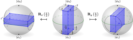
Figure S1: A normal system of roots $z,1/z,-z,-1/z$ together with the conjugate points $\bar{z},1/\bar{z},-\bar{z},-1/\bar{z}$ span the cuboid whose faces are parallel to the $XZ$, $XY$ and $YZ$ planes. There are 24 rotations of the Bloch sphere which preserve this property, composing the elements of the group $\mathcal{G}_{24}$. Two of them, namely the rotation by a $\pi/2$ angle around $X$ and $Y$ axes are presented. The system of roots transforms according to Eqs. S9-S11, giving $z\mapsto z^{\prime}:=\frac{z-i}{-iz+1}$ and $z\mapsto z^{\prime\prime}:=\frac{z-1}{z+1}$ for the two rotations.

Proposition 2.

Each non-degenerated four points $z_{1},z_{2},z_{3},z_{4}$ on the Bloch sphere can be transformed onto the normal form $z,\frac{1}{z},-z,-\frac{1}{z}$ via a Möbius transformation $T$. The latter is uniquely defined up to $24$ rotations in the group $\mathcal{G}_{24}$.

Proof.

For each complex number $\lambda$ there exists another complex number $z$, such that the cross-ratio of the four points is equal to $\lambda$, i.e.

$$\Big{(}z,\frac{1}{z};-z,-\frac{1}{z}\Big{)}=\lambda\,.$$ (S12)

Indeed, the cross-ratio on the left side equals ${4z^{2}}/{(1+z^{2})^{2}}$, and the equation ${4z^{2}}/{(1+z^{2})^{2}}=\lambda$ has exactly four solutions

$$z_{0}=\frac{4-2\lambda+\sqrt{1-\lambda}}{2\lambda},\;\frac{1}{z_{0}},\;-z_{0},\;-\frac{1}{z_{0}}.$$ (S13)

Therefore, for a given value $\lambda$ there exists a unique $\lambda$-normal system, such that the cross-ratio of its vertices is given by $(z_{0},\frac{1}{z_{0}};-z_{0},-\frac{1}{z_{0}})=\lambda$. Replacing the vertex $z_{0}$ by any other vertex $z_{0},{1}/{z_{0}},-z_{0}$, or $-{1}/{z_{0}}$ does not change the value of the cross-ratio $(z_{0},\frac{1}{z_{0}};-z_{0},-\frac{1}{z_{0}})=\lambda$. Note that there exists a unique Möbius transformation $T$ which maps $z_{1},z_{2},z_{3}$ onto $z_{0},{1}/{z_{0}},-z_{0}$, with the remaining $z_{4}$ mapped onto $-{1}/{z_{0}}$. Observe as well that the value of $z_{0}$ is unique up to its inverse, opposite and opposite inverse elements, according to Eq. S13, with the corresponding Möbius transformations associated to the matrices $T,\sigma_{x}T,\sigma_{y}T$ and $\sigma_{z}T$. Each of those transformations maps the set of points $\{z_{1},z_{2},z_{3},z_{4}\}$ onto the same set of points $\{z_{0},{1}/{z_{0}},-z_{0},-{1}/{z_{0}}\}$, although the exact bijection between those two sets of roots is different for each transformation.

Depending on the order of four points $\{z_{1},z_{2},z_{3},z_{4}\}$, the corresponding cross-ratio takes six values: $\lambda,\frac{1}{\lambda},1-\lambda,\frac{1}{1-\lambda},\frac{\lambda-1}{\lambda}$ and $\frac{\lambda}{\lambda-1}$. For each of these, there is a corresponding set of solutions of the form $\{z_{0},{1}/{z_{0}},-z_{0},-{1}/{z_{0}}\}$ via Eq. S13 with four related Möbius transformations. Therefore, there are in total 24 Möbius transformations that map any four non-degenerated points onto a normal system, each of them related by an element of the group $\mathcal{G}_{24}$ which has exactly $24$ elements. ∎

III Section 3. Proof of Proposition 1

Consider the state $\ket{G_{abcd}}$ and its decomposition with respect to the first subsystem $\ket{G_{abcd}}=\ket{0}\ket{\psi_{0}}+\ket{1}\ket{\psi_{1}}$, where

$$\ket{\psi_{0}} =\frac{a+d}{2}\ket{000}+\frac{a-d}{2}\ket{011}+\frac{b+c}{2}\ket{101}+\frac{b-c}{2}\ket{110}\,,$$

$$\ket{\psi_{1}} =\frac{a+d}{2}\ket{111}+\frac{a-d}{2}\ket{100}+\frac{b+c}{2}\ket{010}+\frac{b-c}{2}\ket{001}\,.$$

Suppose that $\tau^{(3)}(\zeta\ket{\psi_{0}}+\ket{\psi_{1}})=0$. Since $\tau^{(3)}$ is a $\text{SL(}2,\mathbb{C}\text{)}^{\otimes 3}$ invariant, for any local operators $\mathcal{O}_{1}$, $\mathcal{O}_{2}$, $\mathcal{O}_{3}$ we have

$$\tau^{(3)}\Big{(}(\mathcal{O}_{1}\otimes\mathcal{O}_{2}\otimes\mathcal{O}_{3})\big{(}\zeta\ket{\psi_{0}}+\ket{\psi_{1}}\big{)}\Big{)}=0\,.$$

Observe that

$$\ket{\psi_{0}}= (\sigma_{x}\otimes\sigma_{x}\otimes\sigma_{x})\ket{\psi_{1}}\,,$$

$$\ket{\psi_{1}}= (\sigma_{x}\otimes\sigma_{x}\otimes\sigma_{x})\ket{\psi_{1}}\,,$$

where $\sigma_{x},\sigma_{y},\sigma_{z}$ are Pauli matrices. Therefore by taking all local operators $\mathcal{O}_{1},\mathcal{O}_{2},\mathcal{O}_{3}$ equal to $\sigma_{x}$, we may conclude that

$$0=\tau^{(3)}\Big{(}(\sigma_{x}\otimes\sigma_{x}\otimes\sigma_{x})\big{(}\zeta\ket{\psi_{0}}+\ket{\psi_{1}}\big{)}\Big{)}=\zeta\ket{\psi_{1}}+\ket{\psi_{0}}\propto\frac{1}{\zeta}\ket{\psi_{0}}+\ket{\psi_{1}},$$ (S14)

hence $1/\zeta$ is another root of $\tau^{(3)}$. Similarly, by considering $(\sigma_{y}\otimes\sigma_{y}\otimes\sigma_{y})$ and $(\sigma_{z}\otimes\sigma_{z}\otimes\sigma_{z})$, one may find another two roots $-\zeta,\;-1/\zeta$ of $\tau^{(3)}$. This shows that the roots of $\tau^{(3)}$ evaluated on any state from the $G_{abcd}$ family are symmetrical with respect to rotations around $X,Y,Z$ axes by the angle $\pi$. Writting $\tau^{(3)}(z\ket{\psi_{0}}+\ket{\psi_{1}})=0$ explicitely, we obtain the equation

$$\tau^{(3)}(z\ket{\psi_{0}}+\ket{\psi_{1}})=Az^{4}-2(2B+A)z^{2}+A=0,$$ (S15)

where $A=(b^{2}-c^{2})(a^{2}-d^{2})$ and $B=(c^{2}-d^{2})(a^{2}-b^{2})$. The above equation is non-degenerated iff $A,B,A+2B\neq 0$, which happens iff $a^{2}\neq b^{2}\neq c^{2}\neq d^{2}$ are pairwise different.

Lemma 1.

Any local operator $\mathcal{O}=\mathcal{O}_{1}\otimes\mathcal{O}_{2}\otimes\mathcal{O}_{3}\otimes\mathcal{O}_{4}\in\text{SL(}2,\mathbb{C}\text{)}^{\otimes 4}$ which transforms states $\ket{G_{a^{\prime}b^{\prime}c^{\prime}d^{\prime}}}\propto\mathcal{O}\ket{G_{abcd}}$ with $a^{2}\neq b^{2}\neq c^{2}\neq d^{2}$, is of the form $\mathcal{O}_{i}\in\mathcal{G}_{24}$.

Proof.

A local operator $\mathcal{O}_{1}$ acting on the first qubit and transforming the state $\ket{G_{abcd}}$ onto $\ket{G_{a^{\prime}b^{\prime}c^{\prime}d^{\prime}}}$, also transforms their systems of roots denoted as $\Lambda$ and $\Lambda^{\prime}$, respectively, via the action of the corresponding Möbius transformation. Note that both systems $\Lambda$ and $\Lambda^{\prime}$ are in the normal form, therefore, according to Proposition 2, we have that $\mathcal{O}_{i}\in\mathcal{G}_{24}$. A similar analysis with respect to all other qubits shows that $\mathcal{O}_{2},\mathcal{O}_{3},\mathcal{O}_{4}\in\mathcal{G}_{24}$. ∎

This way, searching for SLOCC-equivalence between the states $\ket{G_{abcd}}$ and $\ket{G_{a^{\prime}b^{\prime}c^{\prime}d^{\prime}}}$ becomes restricted to the search within the finite class of operators $\mathcal{O}\in\mathcal{G}_{24}^{\otimes 4}$. Since the group $\mathcal{G}_{24}$ has only 24 elements, one may numerically verify that there are exactly $8\times 24=192$ states in the $G_{abcd}$ family which are SLOCC-equivalent to $\ket{G_{abcd}}$ by $\mathcal{O}\in\mathcal{G}_{24}^{\otimes 4}$. For example, the following operation

$$\mathbf{R}_{x}\Big{(}\frac{\pi}{2}\Big{)}\otimes\mathbf{R}_{x}\Big{(}\frac{\pi}{2}\Big{)}\otimes\mathbf{R}_{x}\Big{(}\frac{\pi}{2}\Big{)}\otimes\mathbf{R}_{x}\Big{(}\frac{\pi}{2}\Big{)}$$ (S16)

transforms state $\ket{G_{abcd}}$ into $\ket{G_{-b-acd}}$. This might be simply written as a transformation of a tuples of indices: the tuple $(a,b,c,d)$ is transformed into the tuple $(-b,-a,c,b)$. Similarly, the operators showed on the following right hand sides provide the corresponding transformations of the tuple $(a,b,c,d)$ on the left side:

$$\mathbf{R}_{y}\Big{(}\frac{\pi}{2}\Big{)}\otimes\mathbf{R}_{y}\Big{(}\frac{\pi}{2}\Big{)}\otimes\mathbf{R}_{y}\Big{(}\frac{\pi}{2}\Big{)}\otimes\mathbf{R}_{y}\Big{(}\frac{\pi}{2}\Big{)} \quad\longleftrightarrow\quad(a,{\color[rgb]{0,0,1}d},c,{\color[rgb]{0,0,1}b}),$$

$$\mathbf{R}_{z}\Big{(}\frac{\pi}{2}\Big{)}\otimes\mathbf{R}_{z}\Big{(}\frac{\pi}{2}\Big{)}\otimes\mathbf{R}_{z}\Big{(}\frac{\pi}{2}\Big{)}\otimes\mathbf{R}_{z}\Big{(}\frac{\pi}{2}\Big{)} \quad\longleftrightarrow\quad({\color[rgb]{0,0,1}-d},b,c,{\color[rgb]{0,0,1}-a}),$$

$$\mathbf{R}_{y}({\pi})\otimes\mathbf{R}_{y}({\pi})\otimes\textbf{1}\otimes\textbf{1} \quad\longleftrightarrow\quad(a,{\color[rgb]{0,0,1}-b},{\color[rgb]{0,0,1}-c},d),$$

$$\mathbf{R}_{x}({\pi})\otimes\mathbf{R}_{x}({\pi})\otimes\textbf{1}\otimes\textbf{1} \quad\longleftrightarrow\quad(a,b,{\color[rgb]{0,0,1}-c},{\color[rgb]{0,0,1}-d}),$$

$$\mathbf{R}_{y}({\pi})\otimes\textbf{1}\otimes\mathbf{R}_{y}({\pi})\otimes\textbf{1} \quad\longleftrightarrow\quad({\color[rgb]{0,0,1}d},{\color[rgb]{0,0,1}c},{\color[rgb]{0,0,1}b},{\color[rgb]{0,0,1}a}),$$

$$\mathbf{R}_{x}({\pi})\otimes\textbf{1}\otimes\mathbf{R}_{x}({\pi})\otimes\textbf{1} \quad\longleftrightarrow\quad({\color[rgb]{0,0,1}b},{\color[rgb]{0,0,1}a},{\color[rgb]{0,0,1}d},{\color[rgb]{0,0,1}c})\,.$$

Additionally, the tuples $(a,b,c,d)$ and $(-a,-b,-c,-d)$ represent the same state. Note that any composition of the above operations also provides SLOCC equivalences between $\ket{G_{abcd}}$ states. The eight aforementioned transformations of tuples generate all permutations of the $a,b,c,d$ indices, together with the change of a sign of any two or all four indices. There are exactly $24$ permutations and for each permutation the signs can be matched in exactly $1+{{4}\choose{2}}+1=8$ ways. This gives in total $192$ tuples representing SLOCC equivalent states, which perfectly matches the numerical result.

Finally, another trivial manipulation with indices $a,b,c,d$ comes from multiplying by a global phase, which is an irrelevant operation due the fact that quantum states are elements of a projective space. This operation transforms the indices as

$$(e^{i\theta}a,\;e^{i\theta}b,\;e^{i\theta}c,\;e^{i\theta}d)\sim(a,b,c,d)\,,$$

resulting in the same quantum state for any real number $\theta\in[0,2\pi)$. In particular, for $\theta=\pi$, we observe that system of opposite indices determines the same state as the initial one, i.e. $(-a,-b,-c,-d)\sim(a,b,c,d)$.

References

- Dür et al. (2000) W. Dür, G. Vidal, and J. Cirac, Three qubits can be entangled in two inequivalent ways, Phys. Rev. A 62 (2000).
- Verstraete et al. (2001) F. Verstraete, J. Dehaene, B. De Moor, and H. Verschelde, Four qubits can be entangled in nine different ways, Phys. Rev. A 65 (2001).
- Gour and Wallach (2013) G. Gour and N. Wallach, Classification of multipartite entanglement of all finite dimensionality, Phys. Rev. Lett. 111, 060502 (2013).
- Li et al. (2009) D. Li, X. Li, H. Huang, and X. Li, Slocc classification for nine families of four-qubits, Quantum Info. Comput. 9, 778–800 (2009).
- Viehmann et al. (2011) O. Viehmann, C. Eltschka, and J. Siewert, Polynomial invariants for discrimination and classification of four-qubit entanglement, Phys. Rev. A 83, 052330 (2011).
- Zhang et al. (2016) T. Zhang, M.-J. Zhao, and X. Huang, Criterion for slocc equivalence of multipartite quantum states, Journal of Physics A: Mathematical and Theoretical 49, 405301 (2016).
- Gour and Wallach (2011) G. Gour and N. Wallach, Necessary and sufficient conditions for local manipulation of multipartite pure quantum states, New Journal of Physics 13, 073013 (2011).
- Burchardt and Raissi (2020) A. Burchardt and Z. Raissi, Stochastic local operations with classical communication of absolutely maximally entangled states, Phys. Rev. A 102, 022413 (2020).
- Wootters (1998) W. K. Wootters, Entanglement of formation of an arbitrary state of two qubits, Phys. Rev. Lett. 80, 2245 (1998).
- Coffman et al. (2000a) V. Coffman, J. Kundu, and W. K. Wootters, Distributed entanglement, Physical Review A 61, 052306 (2000a).
- Love et al. (2007) P. Love, A. Brink, A. Smirnov, M. Amin, M. Grajcar, E. Il’ichev, A. Izmalkov, and A. Zagoskin, A characterization of global entanglement, Quantum Information Processing 6, 187 (2007).
- Eltschka and Siewert (2014) C. Eltschka and J. Siewert, Quantifying entanglement resources, Journal of Physics A: Mathematical and Theoretical 47, 424005 (2014).
- Uhlmann (1998) A. Uhlmann, Entropy and optimal decompositions of states relative to a maximal commutative subalgebra, Open Systems & Information Dynamics 5, 209 (1998).
- Tóth et al. (2015) G. Tóth, T. Moroder, and O. Gühne, Evaluating convex roof entanglement measures, Phys. Rev. Lett. 114, 160501 (2015).
- Osborne and Verstraete (2006) T. J. Osborne and F. Verstraete, General monogamy inequality for bipartite qubit entanglement, Physical Review Letters 96 (2006).
- Regula et al. (2014) B. Regula, S. Di Martino, S. Lee, and G. Adesso, Strong monogamy conjecture for multiqubit entanglement: The four-qubit case, Physical Review Letters 113 (2014).
- Regula et al. (2016) B. Regula, A. Osterloh, and G. Adesso, Strong monogamy inequalities for four qubits, Physical Review A 93 (2016).
- Osterloh et al. (2008) A. Osterloh, J. Siewert, and A. Uhlmann, Tangles of superpositions and the convex-roof extension, Phys. Rev. A 77, 032310 (2008).
- Lohmayer et al. (2006) R. Lohmayer, A. Osterloh, J. Siewert, and A. Uhlmann, Entangled three-qubit states without concurrence and three-tangle, Phys. Rev. Lett. 97, 260502 (2006).
- Osterloh (2016) A. Osterloh, Exact zeros of entanglement for arbitrary rank-two mixtures derived from a geometric view of the zero polytope, Phys. Rev. A 94, 062333 (2016).
- Gartzke and Osterloh (2018) S. Gartzke and A. Osterloh, Generalized state of four qubits with exclusively the three-tangle, Phys. Rev. A 98, 052307 (2018).
- Regula and Adesso (2016a) B. Regula and G. Adesso, Entanglement quantification made easy: Polynomial measures invariant under convex decomposition, Phys. Rev. Lett. 116, 070504 (2016a).
- Bengtsson and Zyczkowski (2017) I. Bengtsson and K. Zyczkowski, Geometry of Quantum States: An Introduction to Quantum Entanglement (Cambridge University Press, 2nd edition, 2017).
- Aulbach (2012) M. Aulbach, Classification of entanglement in symmetric states, International Journal of Quantum Information 10, 1230004 (2012).
- Bastin et al. (2009) T. Bastin, S. Krins, P. Mathonet, M. Godefroid, L. Lamata, and E. Solano, Operational families of entanglement classes for symmetricn-qubit states, Physical Review Letters 103 (2009).
- Ribeiro and Mosseri (2011) P. Ribeiro and R. Mosseri, Entanglement in the symmetric sector of qubits, Phys. Rev. Lett. 106, 180502 (2011).
- Kam and Liu (2020) C.-F. Kam and R.-B. Liu, Three-tangle of a general three-qubit state in the representation of majorana stars, Phys. Rev. A 101, 032318 (2020).
- Regula and Adesso (2016b) B. Regula and G. Adesso, Geometric approach to entanglement quantification with polynomial measures, Phys. Rev. A 94, 022324 (2016b).
- Quinta and André (2018) G. M. Quinta and R. André, Classifying quantum entanglement through topological links, Physical Review A 97, 042307 (2018).
- Quinta et al. (2019) G. M. Quinta, R. André, A. Burchardt, and K. Życzkowski, Cut-resistant links and multipartite entanglement resistant to particle loss, Phys. Rev. A 100, 062329 (2019).
- Sudbery (2001) A. Sudbery, On local invariants of pure three-qubit states, Journal of Physics A: Mathematical and General 34, 643 (2001).
- Oleg Chterental (2007) D. Z. D. Oleg Chterental, Linear algebra research advances (Nova Science Publishers, New York, 2007) Chap. 4, pp. 133–167.
- Spee et al. (2016) C. Spee, J. I. de Vicente, and B. Kraus, The maximally entangled set of 4-qubit states, Journal of Mathematical Physics 57, 052201 (2016).
- Coffman et al. (2000b) V. Coffman, J. Kundu, and W. K. Wootters, Distributed entanglement, Phys. Rev. A 61, 052306 (2000b).
- Luque and Thibon (2003) J.-G. Luque and J.-Y. Thibon, Polynomial invariants of four qubits, Phys. Rev. A 67, 042303 (2003).
- Gour and Wallach (2010) G. Gour and N. Wallach, All maximally entangled four-qubit states, Journal of Mathematical Physics 51, 112201 (2010).
- Eltschka et al. (2009) C. Eltschka, A. Osterloh, and J. Siewert, Possibility of generalized monogamy relations for multipartite entanglement beyond three qubits, Physical Review A 80, 10.1103/physreva.80.032313 (2009).
- Eltschka and Siewert (2015) C. Eltschka and J. Siewert, Monogamy equalities for qubit entanglement from lorentz invariance, Phys. Rev. Lett. 114, 140402 (2015).
- Verstraete et al. (2003) F. Verstraete, J. Dehaene, and B. De Moor, Normal forms and entanglement measures for multipartite quantum states, Phys. Rev. A 68, 012103 (2003).