Leveraging Pre-Images to Discover Nonlinear Relationships in Multivariate Environments
††thanks: This research was partly funded by an Ernest J. Del Monte Institute for Neuroscience Award from the Harry T. Mangurian Jr. Foundation. This work was conducted as a Practice Quality Improvement (PQI) project related to American Board of Radiology (ABR) Maintenance of Certificate (MOC) for Prof. Dr. Axel Wismüller. We thank Dr. John Foxe, Institute for Neuroscience, University of Rochester, for his support.
Abstract
Causal discovery, beyond the inference of a network as a collection of connected dots, offers a crucial functionality in scientific discovery using artificial intelligence. The questions that arise in multiple domains, such as physics, physiology, the strategic decision in uncertain environments with multiple agents, climatology, among many others, have roots in causality and reasoning. It became apparent that many real-world temporal observations are nonlinearly related to each other. While the number of observations can be as high as millions of points, the number of temporal samples can be minimal due to ethical or practical reasons, leading to the curse-of-dimensionality in large-scale systems. This paper proposes a novel method using kernel principal component analysis and pre-images to obtain nonlinear dependencies of multivariate time-series data. We show that our method outperforms state-of-the-art causal discovery methods when the observations are restricted by time and are nonlinearly related. Extensive simulations on both real-world and synthetic datasets with various topologies are provided to evaluate our proposed methods.
Index Terms:
causal graphical models, discovering nonlinear interactions, network inference, causality, large-scale time-seriesI INTRODUCTION
Causal relationships are meaningful and apply to many problems, as evidenced by the DARPA’s recent challenge on machine common-sense (MCS) [1]. Such applications require an AI machine with a mechanism to understand and reason the system’s underlying relations, which solo statistics cannot plead (see [2] for the condition that statistics fail). One may argue that such AI machines are causal because AI that finds rules is equivalent to AI that finds causality: when a causal relationship is strong enough, we call it a rule [3, Chapter 1]. An inherent advantage of learning reasons is learning with few samples. Causality gained the most traction recently to build models with sufficient robustness, generalizability, interpretability, and the capability to discover semantically meaningful representations.
The completeness of identifiability and development of do-calculus paved the way for causal inference using observational data [2]. However, using solo temporal measurements, the generative process underneath data is unknown, making the use of do-calculus unsettled. Granger causality (GC) is widely used to infer causality in the time-series data given the faithfulness assumption. GC initially stated for linear relations [4], and states that a time-series A is a cause for time-series B if A causes a better prediction for B.
Although there is a rich body of literature on discovering nonlinear relations from time-series data in the recent decade, yet it is a challenging problem for two reasons: 1) the detected nonlinear relations can be spurious, which requires a multivariate approach, and 2) the curse-of-dimensionality and ill-posedness becomes the main problem with an increasing number of nodes [5, 6]. Various algorithms have been proposed to recover nonlinear relations in networks, including Ancona’s work [7], where they present conditions to detect nonlinear relationships, and in [8] Marinazzo develops a method, called kernel Granger causality (KGC) to consider spurious relations using kernel functions. Unfortunately, their approach in [7] is bivariate and cannot be extended to multivariate settings, and [8] cannot be applied to large-scale problems due to over-fitting. In parallel with the Marinazzo approach, another method called transfer entropy (TE) was proposed by Schreiber [9], which formulates the causal relationship among time-series from the information theory’s perspective. In his 2009 paper, Barnett proved that the TE and GC were equivalent for Gaussian variables [10]. Therefore, the KGC under the Gaussian assumption is equal to TE. These two lines of work (TE and KGC) have received considerable attention.
Several algorithms have been proposed to extended the previously discussed approaches to multivariate time-series [11, 12, 5, 13, 14, 15]; however, the curse-of-dimensionality of the large-scale problem yet is an open problem [5]. Note that in real-world studies such as climatology, the dimensions of the problem can reach millions of variables [16], so in the presence of short time-series (just a few decades of temperature measurement), the inverse problems quickly become ill-posed due to the presence of redundant variables. In large-scale problems, TE-based methods are costly based on their dependency on estimating the probability distribution functions. Our analysis of a recent TE algorithm based on the Kraskov estimation [12] for a graph with 34 nodes takes 26 hours on an Nvidia GeForce 1080-Ti GPU and tens of times more on a CPU, while the cost increases drastically with the number of nodes.
The closest study to our work in terms of the ongoing open problem is the PCMCI method [5]. Peter and Clark Momentary Conditional Independence (PCMCI) is a two-step algorithm, with an statistical independence test in the PC stage, and obtaining causality strengths of the significant links in the MCI stage [5]. Besides, because our method is a nonlinear Granger causality under Gaussian assumption, it is equivalent to the TE [12, 11, 10] for Gaussian variables. However, our proposed method differs from the above methods in two ways. First, since it is a nonlinear GC method, it is equivalent to the TE method for Gaussian variables, while it is also suitable for large-scale problems. On the other hand, although PCMCI is proposed for large-scale problems, the method we present provides the ability to apply to short time-series on a large scale and provides all steps without examining nonlinear independencies using a partial correlation as is in the PCMCI. We believe our contribution adds numerous capabilities to the existing literature, affirmed through extensive simulations on synthetic and real-world datasets.
II PRELIMINARIES
In an abuse of notation, we use and to point to the nodes and random variables on the nodes. Scalars are small letters, vectors are in small bold letters, and matrices are in bold capital letters. Calligraphic letters , and represent the set of nodes, set of weighted edges, feature space (Hilbert subspace), and input space, correspondingly.
Causality assumptions
A variable is said to be a cause of a variable if can change in response to change in . Consider a directional graphical model consisting of the set of nodes and the set of directed edges , whose topology is unknown, but time-series are observed per node , over time intervals. We assume that edges are causal, meaning that every parent is a direct cause of all its children , and therefore is a parent of , denoting as . Furthermore, we assume that measurements are causally sufficient, meaning that there are no unobserved confounders of any of the variables in the graph111Note that we cannot test unconfoundedness, and cannot guarantee that it is satisfied. In other words, no unobserved confounding is unrealistic assumption, and we will always have unobserved confounders [17]. Our goal is to estimate causal quantities between each pair of the nodes and in the presence of all other nodes , and derive the topology of the graph as , such that . We assume that is identifiable, therefore we can compute it from a purely statistical quantity222Identifiablity requires to have four assumptions: unconfoundness, positivity, consistency, and no interference.[2]. We use faithfulness assumption to obtain causal relations among the nodes , which allows us to infer d-separations in the graph from in dependencies in the distributions . The notion implies independence in the graph , or the distribution where denotes the random variable corresponding to node . Note that faithfulness is a weak assumption; however, without it, we cannot infer the topology of the causal graph from the observational time-series333The reason is related to global Markov assumption, where given that P is Markov with respect to graph one can use to infer independencies in . However, in case of the unstructured time-series data, the graph topology is priory unknown and we cannot use Markov assumption before obtaining the graph topology..
Causal quantities
Linear vector autoregressive model (VARM) is widely adopted framework to infer Granger causality in multivariate time-series, in which a Granger causality index can be defined as a quantification of prediction quality as follows. VARM states that each observed is a linear combination of the time-lagged versions of the measurements . Let denote the “time-lagged” VARM parameters matrix, with , and as model coefficients over a lag of time points. Given the time-lagged multivariate time-series , where , the goal is to estimate the model parameter matrices in:
| (1) |
and minimize the residual errors using an optimization method, such as ordinary least squares (OLS), the lasso, the ridge, or the elastic-net regressions [18].
Let be the matrix of residuals of VARM for the full system including all nodes , and let to be the same matrix when the node is excluded from the VARM, where each is obtained using in expression (1). Then, the derivation of error covariance matrices and will be straightforward. Based on of the full VARM and of the VARM without , the degree of information flow from node to node can be quantified by , where and denote the diagonal entries of and associated to node , respectively. Consequently, the topology of the causal graph can be inferred using:
| (2) |
as .
Problem Statement
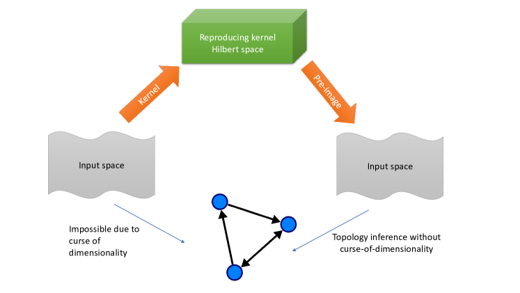
Given nodal measurements in (1), the aim is to solve VARM in the reproducing kernel Hilbert space (RKHS) and then revert the solution (residuals) to the input space to infer the topology in the input space. The benefit is to encompass nonlinearities while reducing dimensionality to address the curse-of-dimensionality.
III The proposed method
The proposed method consists of three steps using three off-the-shelf modules, as shown in Fig. 1. The first step involves a transformation of the input space to the dimensionality reduced (or lifted) feature space using kernel principal component (kernel PCA), the second step involves solving the VARM of (1) in the feature space, and the third step which is the essential part of the method, is to revert the residuals of the VARM in the feature space into the input space using pre-images, and finally infer the topology of the graph in the input space.
Dimensionality reduction using kernel PCA
The aim is to transfer the equation (1) to the space of the principal components with lower dimensions, encompassing nonlinear dependencies. We define RKHS function as to project time-series measurements into the feature space. A feature space related to the principal components with the maximum explained variance of data would be desired; therefore, kernel PCA is of interest. Altough as the dimension of the feature space is desired, can be also used to to lift the space (rather than reducing). Therefore, builds the basis of feature space, and . A projection of input data onto the -th principal component would be desired, such that the major proportion of data variation is explained by a few principal components [19].
Solving the VARM in the reproducing kernel Hilbert space
Using the RKHS function transformation, the feature space representation of (1) will be:
| (3) |
where for is the transformed time-series into the feature space, and is the error at time slot in the feature space. The expression (3) is a linear VARM and can be derived with the same approach as discussed in section II. Once the in (3) are obtained , the predictions will be transformed into the input space to infer the graph topology.
Estimating pre-images
Let , , , , , , and , and the notations , , for the sake of simplicity. To transform into the input space and obtain the pre-image , one needs to estimate , which is a nonlinear optimization problem, and is not interesting as a solution to find pre-images [19, 20]. However, interestingly, both the inputs and their corresponding mappings are present for , easing the pre-image problem to a simple learning problem. Therefore, we use the learning problem instead, which is adopted from [20] to directly obtain coefficients , and consequently the predictions will be obtained. Simultaneously, the topology of the graph can be obtained as discussed in section II. The complete algorithm is shown in Algorithm. 1. Note that novel statistical frameworks such as [21, 22, 23, 24] can be used to formulate the problem in a neural network, which can be as a future work.

IV Numerical Tests
Extensive simulations on a benchmark of the synthetic datasets with known ground-truth and a real-world dataset in a downstream task are presented in this section.
Tests on synthetic datasets
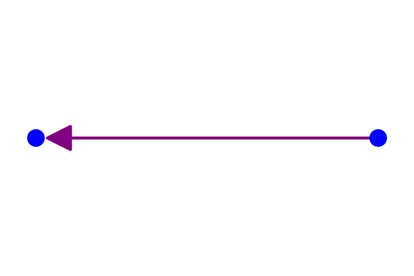
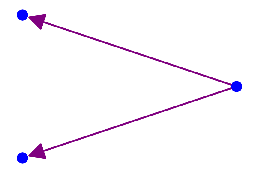
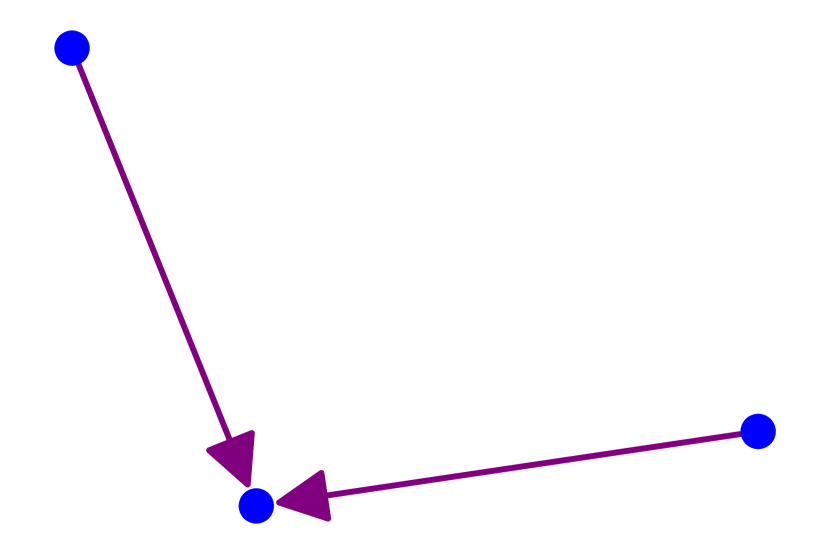
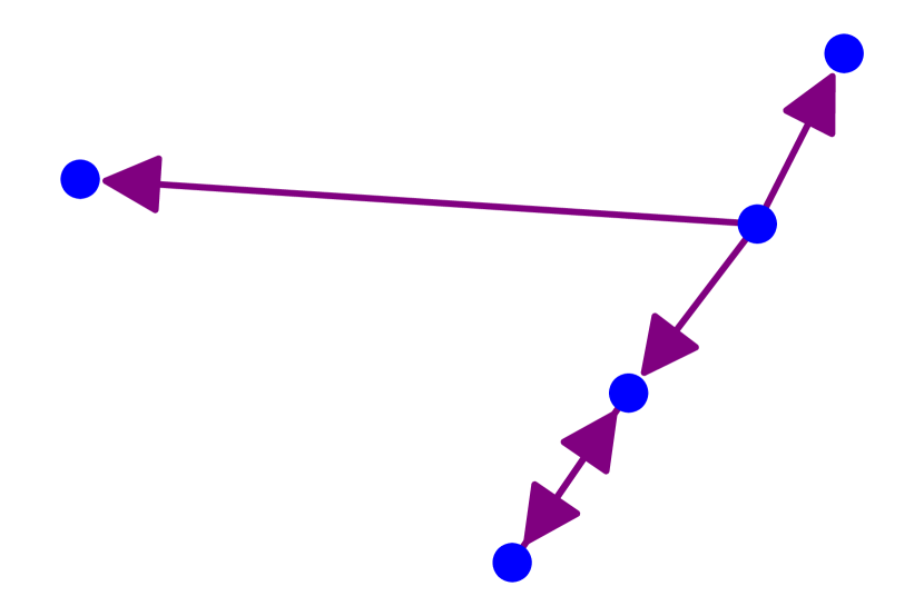
We used five various networks with various topologies, each with 50 random realizations, to test our method and some of the state-of-the-art methods, namely PCMCI (2019) [5], mutual information using Kraskov estimation (2018) [12], transfer entropy (TE) using Kraskov method (2018) [11, 12], and kernel Granger causality 2011[13]. The topology of the datasets are shown in Fig. 2. We used one 2-nodes chaotic master-slave, two 3-nodes with fork and immorality topologies, and two 5-nodes datasets in the linear and nonlinear dependencies mode. Datasets are detailed in [25].
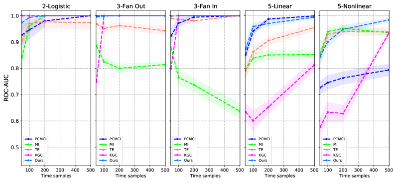
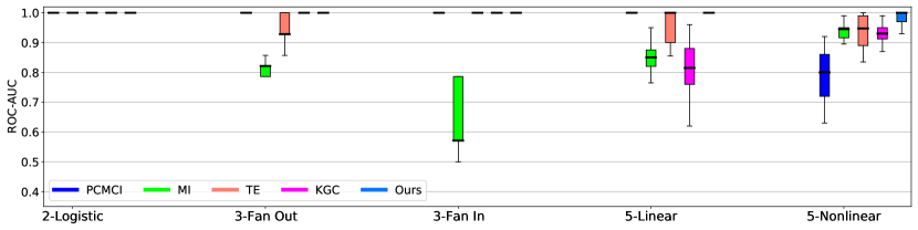
We used datasets to address two challenges: 1) Fig. 3 shows the case of which datasets have enough time samples for different topologies, and 2) Fig. 4 shows when the trend of different algorithms by reducing the number of time samples. ROC-AUC is used to compare the performance in the box plots. It is clearly seen in Fig. 3 and 4 that our algorithm is more robust to the size of the network, nonlinearity in dependencies, and short time-series. Note that PCMCI is also proposed for large-scale problems, but in our simulations, we show that our algorithm’s robustness for short time-series is better than the PCMCI.
Tests on real datasets
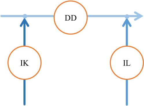
We examine our method on climatology data of average daily discharges of rivers in the upper Danube basin by three stations located on the Iller at Kempten (IK), the Danube at Dillingen (DD), and the Isar at Lenggries (IL). The data are available through Bavarian Environmental Agency at https://www.gkd.bayern.de, and we use the measurements of three years (2017-2019). As shown in Fig. 5, there is a causal relationship IK DD since IK discharges into the DD upstream after a day, while there is no causal relationship between ILIK and ILDD (and vice versa). Due to confounder variables such as rainfall or other weather conditions, the statistical analyses are vulnerable to detecting spurious connections. Our method correctly detects a causal relationship between IK and DD while detecting no relationships between IL-IK and IL-DD, unconfounding spurious variables. In contrast, the Kraskov’s TE [12, 9] wrongly detects the spurious connections as the DDIK, DDIL, ILIK, and ILDD altogether, for the best parameters. Our analysis of rivers’ underlying dynamics conforms to [26], which shows our method’s capability to distinguish between confounding and causal variables.
V Conclusions
This paper puts forth a novel method for discovering nonlinear dependencies between time-series in multivariate environments. The method aims to solve curse-of-dimensionality while preserving nonlinear dependencies using combination of kernel principal component analysis, linear vector autoregressive model, and estimating pre-images to obtain topology of the graph in the input space. The method’s advantage is its simplicity, while the results on the synthetic and real-world datasets show the merit of the method compared to state-of-the-art causality inference methods.
References
- [1] M. Turek. Machine Common Sense. . [Online]. Available: https://www.darpa.mil/program/machine-common-sense
- [2] I. Shpitser and J. Pearl, “Complete Identification Methods for the Causal Hierarchy,” Journal of Machine Learning Research, Vol. 9, pp. 1941–1979, September 2008.
- [3] J. Pearl and D. Mackenzie, The Book of Why: the New Science of Cause and Effect. Basic Books, 2018.
- [4] C. Granger, “Some Recent Development in a Concept of Causality,” Journal of Econometrics, Vol. 39, No. 1-2, pp. 199–211, September 1988.
- [5] J. Runge et al., “Detecting and Quantifying Causal Associations in Large Nonlinear Time Series Datasets,” Science Advances, Vol. 5, No. 11, pp. 1–15, November 2019.
- [6] Y. Antonacci, L. Astolfi, and L. Faes, “Testing Different Methodologies for Granger Causality Estimation: A Simulation Study,” in European Signal Processing Conference, January 2021, pp. 940–944.
- [7] N. Ancona, D. Marinazzo, and S. Stramaglia, “Radial Basis Function Approach to Nonlinear Granger Causality of Time Series,” Physical Review E, Vol. 70, No. 5, pp. 1–7, November 2004.
- [8] D. Marinazzo, M. Pellicoro, and S. Stramaglia, “Kernel-Granger Causality and the Analysis of Dynamical Networks,” Physical review E, Vol. 77, No. 5, pp. 1–9, May 2008.
- [9] T. Schreiber, “Measuring Information Transfer,” Physical Review Letters, Vol. 85, No. 2, pp. 1–4, July 2000.
- [10] L. Barnett, A. B. Barrett, and A. Seth, “Granger Causality and Transfer Entropy are Equivalent for Gaussian Variables,” Physical Review Letters, Vol. 103, No. 23, pp. 1–4, December 2009.
- [11] A. Kraskov, H. Stögbauer, and P. Grassberger, “Estimating Mutual Information,” Physical Review E, Vol. 69, No. 6, pp. 1–16, June 2004.
- [12] L. Novelli et al., “Large-Scale Directed Network Inference with Multivariate Transfer Entropy and Hierarchical Statistical Testing,” MIT Press, Vol. 3, No. 3, pp. 827–847, July 2019.
- [13] D. Marinazzo et al., “Nonlinear Connectivity by Granger Causality,” Neuroimage, Vol. 58, No. 2, pp. 330–338, September 2011.
- [14] J. Runge et al., “Inferring Causation from Time Series in Earth System Sciences,” Nature Communications, Vol. 10, No. 1, pp. 1–13, June 2019.
- [15] M. A. Vosoughi and A. Wismüller, “Large-scale extended Granger causality for classification of marijuana users from functional MRI,” in Medical Imaging 2021: Biomedical Applications in Molecular, Structural, and Functional Imaging, Vol. 11600, International Society for Optics and Photonics. SPIE, February 2021, pp. 72 – 84.
- [16] G. Camps-Valls, D. Sejdinovic, J. Runge, and M. Reichstein, “A Perspective on Gaussian Processes for Earth Observation,” National Science Review, Vol. 6, No. 4, pp. 616–618, July 2019.
- [17] C. Manski, Partial Identification of Probability Distributions. Springer Science & Business Media, 2003.
- [18] J. Friedman, T. Hastie, and R. Tibshirani, “Regularization Paths for Generalized Linear Models via Coordinate Descent,” Journal of Statistical Software, Vol. 33, No. 1, p. 1, August 2010.
- [19] B. Schölkopf et al., Learning with Kernels: Support Vector Machines, Regularization, Optimization, and Beyond. MIT press, 2002.
- [20] G. Bakır, J. Weston, and B. Schölkopf, “Learning to Find Pre-Images,” pp. 449–456, December 2003.
- [21] N. Mohammadi, M. M. Doyley, and M. Cetin, “Finite element reconstruction of stiffness images in mr elastography using statistical physical forward modeling and proximal optimization methods,” arXiv preprint arXiv:2103.14632, 2021.
- [22] N. Mohammadi et al., “Ultrasound elasticity imaging using physics-based models and learning-based plug-and-play priors,” in ICASSP 2021-2021 IEEE International Conference on Acoustics, Speech and Signal Processing (ICASSP). IEEE, 2021, pp. 1165–1169.
- [23] N. Mohammadi, M. M. Doyley, and M. Cetin, “A statistical framework for model-based inverse problems in ultrasound elastography,” arXiv preprint arXiv:2010.10729, 2020.
- [24] N. Mohammadi, M. M. Doyley et al., “Mr elasticity reconstruction using statistical physical modeling and explicit data-driven denoising regularizer,” arXiv preprint arXiv:2105.12922, 2021.
- [25] A. Wismüller et al., “Large-scale nonlinear Granger causality for inferring directed dependence from short multivariate time-series data,” Scientific Reports, Vol. 11, No. 1, pp. 1–11, 2021.
- [26] L. Mhalla, V. Chavez-Demoulin, and D. J. Dupuis, “Causal Mechanism of Extreme River Discharges in the Upper Danube Basin Network,” Journal of the Royal Statistical Society: Series C (Applied Statistics), Vol. 69, No. 4, pp. 741–764, August 2020.