Invariant Policy Learning: A Causal Perspective
Emails: {ss, thams, jonas.peters, np}@math.ku.dk)
Abstract
Contextual bandit and reinforcement learning algorithms have been successfully used in various interactive learning systems such as online advertising, recommender systems, and dynamic pricing. However, they have yet to be widely adopted in high-stakes application domains, such as healthcare. One reason may be that existing approaches assume that the underlying mechanisms are static in the sense that they do not change over different environments. In many real-world systems, however, the mechanisms are subject to shifts across environments which may invalidate the static environment assumption. In this paper, we take a step toward tackling the problem of environmental shifts considering the framework of offline contextual bandits. We view the environmental shift problem through the lens of causality and propose multi-environment contextual bandits that allow for changes in the underlying mechanisms. We adopt the concept of invariance from the causality literature and introduce the notion of policy invariance. We argue that policy invariance is only relevant if unobserved variables are present and show that, in that case, an optimal invariant policy is guaranteed to generalize across environments under suitable assumptions. Our results establish concrete connections among causality, invariance, and contextual bandits.
1 Introduction
The problem of learning decision-making policies lies at the heart of learning systems. To adopt these learning systems in high-stakes application domains such as personalized medicine or autonomous driving, it is crucial that the learned policies are reliable even in environments that have never been encountered before. In this paper, we consider the problem of learning policies that are robust with respect to shifts across environments. We consider this question in the setup of offline contextual bandits, which provides a mathematical framework for tackling the above learning problems.
While recent studies in offline contextual bandits (Dudik et al., 2011; Bottou et al., 2013; Swaminathan and Joachims, 2015a; Swaminathan and Joachims, 2015b; Kallus, 2018; Athey and Wager, 2021; Zhou et al., 2022) offer theoretical results and novel methodologies for policy learning from offline data, they primarily focus on a fixed-environment setting (from now on, we will refer to this as the equal distribution assumption) in which the underlying mechanisms do not change over time or over different environments. In practice, however, shifts between environments often occur, possibly invalidating the equal distribution assumption. In healthcare, for example, datasets from different hospitals may not come from the same underlying distribution. As a result, a learning agent that ignores environmental shifts may fail to generalize beyond the environments it was trained on.
In the supervised learning context, the environmental shift problem has been studied under different names, such as domain generalization, covariate shift adaptation, distributional robustness or out-of-distribution generalization (Sugiyama and Kawanabe, 2012; Muandet et al., 2013; Volpi et al., 2018; Arjovsky et al., 2019; Christiansen et al., 2021). In domain generalization, the goal is to develop learning algorithms that are robust to changes in the test distribution. Thus, a fundamental problem is how to characterize such changes. A promising direction relies on a causal framework to describe the changes through the concept of interventions (Schölkopf et al., 2012; Rojas-Carulla et al., 2018a; Magliacane et al., 2018; Arjovsky et al., 2019; Christiansen et al., 2021). A key insight is that while purely predictive methods perform best if test and training distributions coincide, causal models generalize to arbitrarily strong interventions on the covariates because of the modularity property of structural causal models (see e.g., Pearl (2009)).
In real-world applications knowledge of the underlying causal graph and structural discrepancies between environments may not be available. In recent years, invariance-based methods have been exploited to learn the causal structure from data (Peters et al., 2016; Pfister et al., 2018; Heinze-Deml et al., 2018). In invariant causal prediction (Peters et al., 2016), for example, one assumes that the data are collected from different environments, each of which describes different underlying data-generating mechanisms, and uses this heterogeneity to learn the causal parents of an outcome variable . The underpinning assumption is the invariance assumption, which posits the existence of a set of covariates in which the mechanism between and remains constant. A model based on such invariant covariates is guaranteed to generalize to all unseen environments.
Our paper delineates an explicit connection among causality, invariance, and the environmental shift problem in the context of contextual bandits. We develop a causal framework for characterizing the environmental shift problem, and provide a practical and theoretically sound solution based on the proposed framework.
Our contributions are threefold. First, we propose a multi-environment contextual bandit framework that represents mechanisms underlying a contextual bandit problem by structural causal models (SCMs; Pearl (2009)). The framework allows for changes in environments and thereby relaxes the equal distribution assumption. We define environments as different perturbations on the underlying SCM, and we evaluate the policy according to its worst-case performance in all environments. Second, using the proposed framework, we generalize the invariance assumption used in methods such as invariant causal prediction and define invariance properties for policies that, under certain assumptions, guarantee generalizability to unseen environments. Third, we develop an offline method for testing invariance under distributional (policy) shifts, and provide an algorithm for finding an optimal invariant policy. In addition, we highlight a setting in which causality and invariance are not necessary for solving the environmental shift problem. This insight takes us closer to understanding what causality can offer in offline contextual bandits.
The remainder of our paper is organized as follows. Sections 1.1 and 1.2 briefly review related work and introduces the offline contextual bandit problem. Section 2 formally defines a causal framework for multi-environment contextual bandits and the main objective of our problem’s formulation. Drawing on the proposed framework, Section 3 introduces invariance properties for policies and provides the main theoretical contributions underpinning our solution for the environmental shift problem. Section 4 discusses the assumptions required to learn invariant policies from offline data and presents an algorithm for learning an optimal invariant policy. Section 5 provides simulation experiments that empirically verify our theoretical results. In Section 6, we apply our framework to a warfarin dosing study.
1.1 Related Work
Our work is most closely related to the line of work studying invariance and generalizability for prediction tasks in i.i.d. settings mentioned above (Rojas-Carulla et al., 2018a; Magliacane et al., 2018; Arjovsky et al., 2019; Christiansen et al., 2021; Pfister et al., 2021). The environmental shift problem is also related to the problem of transportability in causal inference (Pearl and Bareinboim, 2011; Bareinboim and Pearl, 2014, 2016; Subbaswamy et al., 2019; Lee et al., 2020; Correa and Bareinboim, 2020) which aims to generalize causal findings from source environments to a target environment. Our work differs from the transportability literature: we neither assume prior knowledge of the underlying causal graph nor of the structural differences between environments. Instead, we only assume that invariances in the observed environments are preserved in the target environment. Furthermore, while the goal in transportability is to derive whether and how one can identify a causal quantity (e.g., an interventional distribution) in the target environment based on data from the source environment, our goal is to learn worst-case optimal policies based on the source environments.
Graphical models have been used in reinforcement learning to represent the underlying Markov Decision Processes (MDP) under the framework of factored MDPs. Such methods, however, focus mainly on providing efficient planning algorithms rather than generalizing to a new environment (Kearns and Koller, 1999; Guestrin et al., 2003, 2002; Jonsson and Barto, 2006). Although some recent studies have explored the use of causality and invariance for tackling the environmental shift problem in contextual bandits and, more generally, reinforcement learning (Zhang et al., 2020; Sonar et al., 2021), the actual roles and benefits of causality and invariance remain unclear and under-explored.
Our framework differs from the framework of causal bandits (Lee and Bareinboim, 2018; Lattimore et al., 2016; Yabe et al., 2018; de Kroon et al., 2020). While causal bandits exploit causal knowledge (either assumed to be known a priori or estimated from data) for improving the finite sample performance in a single environment, our framework focuses on modeling distributional shifts and the ability to generalize to new environments. Another line of work has addressed the problem of policy evaluation and learning under unobserved confounding between the action and the reward variables (Bareinboim et al., 2015; Sen et al., 2017; Tennenholtz et al., 2020; Kallus and Zhou, 2020; Tennenholtz et al., 2021). In contrast, we consider the complementary problem of unobserved confounding between the covariates and the reward variables (see Section 3).
1.2 Offline Contextual Bandits
We briefly review the offline contextual bandit problem (Beygelzimer and Langford, 2009; Strehl et al., 2010), considering a setup in which some of the covariates (also known as context variables) are unobserved. More precisely, we assume that the covariates can be partitioned into observed and unobserved variables and . Here, and are metric spaces; the reader may think of and . As in the standard contextual bandit setup (Langford and Zhang, 2008), for each round, we assume that the system generates a covariate vector and reveals only the observable to an agent. From the observed covariates , the agent selects an action according to a policy that maps the observed covariates to the probability simplex over the set of actions . (In this work, we assume to be finite). Adapting commonly used notation, we write, for all and , . The agent then receives a reward depending on the chosen action , and on both the observed and unobserved covariates .
In the classical setting, one assumes that the covariates are drawn i.i.d. from a joint distribution (an assumption we will relax when introducing multi-environment contextual bandits in Section 2) and that the rewards are drawn from a conditional distribution . The agent is evaluated based on the performance of its policy which is measured by the policy value:
The agent is now given a fixed training dataset that is collected offline: it consists of rounds from one or more different policies, i.e., , where 111We assume knowledge of the initial policy to ease our presentation and focus our contribution on the environmental shifts problem. Our theoretical results and algorithms remain unchanged even if the initial policy is unknown and needs to be estimated from the offline data (see Appendix F for more details). for all . The goal of the agent is then to find a policy that maximizes the policy value over a given policy class , i.e., .
As mentioned, this setting assumes that the environment in which we deploy the agent is identical to the environment in which the training dataset was collected. Section 2 introduces a causal framework for multi-environment contextual bandits, a framework that relaxes the equal distribution assumption.
2 A Causal Framework for Multi-environment Contextual Bandits
Instead of having a fixed distribution over the covariates, we introduce a collection of environments such that, in each round, the covariates are drawn from an environment-specific distribution that depends on the environment in that round.
In practice, the agent only observes part of the environments and is expected to generalize well to all environments in including the unseen environments . To formalize the problem, we first introduce a model that puts assumptions on how environments change the distributions of , and . Specifically, an environment can only perturb the distribution of the reward through altering the distribution of the covariates and . This constraint makes it possible to generalize information learned from one set of environments to another. In this formulation – even though the full conditional distribution of the reward is assumed to be fixed across environments – the observable distribution after marginalizing out the unobserved may change from one environment to another (see, e.g., Figure 1(b))
Formally, the assumptions are constructed via an underlying class of SCMs indexed by the environment and policy.222 Readers familiar with the standard notion of SCMs may think about an SCM with a source node . then corresponds to an intervention on the action variable (change of policy) and on some of the observed covariates variables (change of environment). Here, we consider fixed environments, so that we do not have to consider them as random draws from an underlying distribution; see also Dawid (2002).
Setting 1 (Multi-environment (acyclic) SCMs for bandits).
Let and be products of metric spaces, a discrete action space, the set of all policies, and a collection of environments. For all and all we consider the following SCMs,
| (1) |
where , , , and are measurable functions, is a random vector with independent components and a distribution , and and are such that for all it holds that is a random variable on with distribution . Figure 1(a) visualizes the coarse-grained structure of this setting. and should be thought of as random vectors. Accordingly, , for example, is a function with a multivariate output; it is a short-hand notation in the sense that a component of does not need to depend on all , for example. In particular, we assume that the graph (defined below) corresponding to the SCMs is acyclic, see Figure 1(b) and 1(c) for an example.
We assume there exists a probability measure on such that for all and all the SCM induces a unique distribution over (see Bongers et al. (2016) for details) which is dominated by and marginally has full support on . We denote the corresponding density by and the corresponding expectations by . Whenever a probability, density, or expectation does not depend on , we omit and write rather than , for example.
Some remarks regarding Setting 1 are in order: (1) We only use the SCMs as a flexible way of modeling the changes in the joint distribution with respect to the environment and the policy . In particular, we do not use it to model any further intervention distributions that do not correspond to a change of policy or environment. (2) In practice, the precise form of the SCMs is unknown. Indeed, we will neither assume knowledge of the structural equations nor complete knowledge of the graph structure, except that the constraints induced by (1) hold. (3) The assumption of a dominating measure for all environments ensures that we can always assume the existence of densities while also switching across environments. In particular, this avoids any measure-theoretic difficulties regarding conditional distributions. (4) The assumption that the induced distributions over have full support in all environments ensures that the generalization problem when moving from to does not involve any extrapolation. Additionally, it ensures that conditional expectations such as can be uniquely defined for all as integrals of the conditional densities. (5) The environments are modelled fixed (and not random). However, we could also treat the environments as random variables which can be considered a special case of the fixed-environment setting (see Appendix E).
We now introduce the graph over the variables that visualizes the structure of the SCMs (for all and ). We draw edges corresponding to the assignments in (1), add edges from all to and add an environment node, which has edges into all variables whose assignments are not the same in all environments. This is similar to the selection diagrams in Pearl and Bareinboim (2011), with the difference that we consider multiple environments.
More precisely, is constructed as follows: Each coordinate of the variables corresponds to a node. The nodes are connected according to the assignments, that is, we draw a directed edge from a variable to a variable if, for at least one environment , the variable appears on the right-hand side of the assignment of variable (see Figure 1(b) for an example). Let and index the variables and for which the structural assignments and in (1) vary with , i.e., where there exist such that or , respectively. The environments correspond to perturbations on variables or , which implies that for each the distribution may vary. We augment the graph with a square node to represent the environments and draw a directed edge from the node to each of the perturbation targets and . Furthermore, we draw edges from all nodes in to and mark them with (to represent their dependence on the policy). This graph is assumed to be acyclic, that is, to not contain any directed cycles. By the Markov condition, which holds in SCMs (Peters et al., 2017), the graph defined above encodes (conditional) independence statements, which we will see relate to invariance, through the concept of -separation. More precisely, the Markov condition states that any -separation statement in a graph implies conditional independence (Pearl, 2009; Lauritzen et al., 1990; Peters et al., 2017). Here, we refer to the standard definition of -separation when not distinguishing between the different types of nodes and denote by a -separation statement in a graph . For completeness, we define -separation in Appendix A.
For any , we also define as the subgraph of , in which, instead of all , only the covariates in point into :
| (2) |
Neither nor depends on the choice of policy.
We are now ready to define contextual bandits with multiple environments.
Definition 1 (Multi-environment Contextual Bandits).
Assume Setting 1. In a multi-environment contextual bandit setup, before the beginning of each round, the system is in an environment . Then, the system generates a covariate vector and reveals only the observable and the environment label to the agent. Based on the observed covariates , the agent selects an action according to the policy . The agent then receives a reward , depending on the chosen action and on both the observed and unobserved covariates . More precisely, we assume for all that are sampled independently according to (see Setting 1). The training data contains data from environments in . When , the setup reduces to a standard contextual bandit setup.
In the multi-environment contextual bandit setup, the covariates on different rounds are not identically distributed due to changes in the environments. We can thus use this framework to model situations, where the test environments differ from training environments. We illustrate this setting with the following example, which we will refer back to several times throughout the paper.
Example 1.
Consider a linear multi-environment contextual bandit with the following underlying SCMs
where are jointly independent noise variables with zero mean, for all , , and . Figure 1(b) depicts the induced graph . In this example, the environments influence the observed covariates in two ways: (a) they change the mean of via and (b) they change the conditional mean of given via , while the rest of the components remain fixed across different environments. Here, the environment-specific coefficient modifies the correlation between the observable and the unobserved variable , and consequently between and the reward . Thus, an agent that uses information from to predict the reward in the training environments may fail to generalize to other environments. To see this, consider a training environment and a test environment and let , be the environment-specific coefficients in the training and test environments, respectively. In the training environment, we have a large positive correlation between and , and consequently the agent will learn that the action yields a higher expected reward when observing a positive value of (and otherwise). However, the correlation between and becomes negative (and large in absolute value) in the test environment, which means that the policy that the agent learned from the training environment will now be harmful. We will see in Section 3 that a policy that depends on a -invariant set ( in this example) does not suffer from this generalization problem and is guaranteed to generalize across different environments.
A similar structure appears in the medical example discussed in Section 6. There, is the dose of a drug, is a response variable, are observed patient features and are unobserved genetic factors. The environment is (a proxy of) the continent on which the data was collected.
2.1 Distributionally Robust Policies
To evaluate the performance of an agent across different environments, we define a policy value that takes into account environments. In particular, we focus on the worst-case performance of an agent across environments.
Definition 2 (Robust Policy Value).
For a fixed policy , and a set of environments , we define the robust policy value as the worst-case expected reward
| (3) |
Intuitively, an agent that maximizes the robust policy value is expected to perform well (relative to other agents) in the most harmful environment. The idea of optimizing worst-case performance has been suggested in the reinforcement learning literature (Garcıa and Fernández, 2015; Amodei et al., 2016) to ensure safe behavior of an agent and prevent catastrophic events and has also been used to formulate adversarial training (Bai et al., 2021) as well as out-of-distribution generalization (Ye et al., 2021).
We now assume that, for several observed environments, we are given an i.i.d. sample from a multi-environment contextual bandit, see Definition 1. More precisely, we assume to observe , where , , for all . Using only , we aim to solve the following maximin problem333The maximum can always be attained when is an unrestricted policy class and takes a form similar to (21).:
| (4) |
If we do not observe all the environments, solving the maximin problem (4) is impossible without further assumptions. A baseline approach to this problem is to pool the data from all training environments and learn a policy that maximizes the policy value ignoring the environment structure. We show in Appendix B that this is indeed optimal if the observed covariates explain all of the environment based distributional shifts in , e.g., if all relevant covariates have been observed. However, if for example, hidden variables are present, the pooling approach does not necessarily yield an optimal policy and the learned policy may fail to generalize to unseen test environments.
3 Invariant Policies for Distributional Robustness
We now consider the general case in which the environment shifts may not be explained by the observed covariates. To this end, we introduce -invariant sets and policies, and show that, under Setting 1, the maximin problem (4) can be reduced to finding an optimal -invariant policy given certain assumptions, see Proposition 1 and Theorem 1. This becomes particularly relevant if important variables remain unobserved. If all variables are observed, it suffices to pool the observed environments.
Remark 1.
Nevertheless, in more realistic cases (see e.g., Figures 1(b) and 1(c)), -invariant sets and policies (introduced below) play a central role in solving the distributionally robust objective (4).
Definition 3 (-invariant Sets444The notion of -invariant sets is related to -admissibility in Pearl and Bareinboim (2011). We use the term ‘-invariant’ to emphasize that the definition is based on the -separation statement (6) and involves the unseen environments. In related contexts, sometimes the term ‘generalizing’ is used (Pfister et al., 2019). Section 4 introduces the invariance hypothesis (12) that is testable from the observed data and discusses the assumptions required to connect the two conditions.).
A subset is said to be -invariant if the following -separation statement holds:
| (5) |
where is defined in (2).
Our approach relies on the existence of a -invariant set. We therefore make this assumption explicit.
Assumption 1.
There exists a subset such that is -invariant.
Under faithfulness (Pearl, 2009), Assumption 1 is testable from the observed data (see Section 4.1). Next, we define -invariant policies. For all subsets , let us denote the set of all policies that depend only on by .
Definition 4 (-invariant Policies).
A policy is said to be -invariant with respect to a subset if is a -invariant set and .
We denote by the collection of all -invariant sets and the collection of -invariant policies. For now, we assume to have access to the set of -invariant policies . Section 4 discusses when and how we can learn from the observed data.
Because of the hidden variables , the conditional mean is not ensured to be stable across the environments. Nevertheless, a -invariant policy ensures that parts of the conditional mean are unchanged across environments.
Lemma 1.
Let be a -invariant set and . It holds for all and that
| (6) |
Proof.
See Appendix D.3. ∎
For , Lemma 1 implies that if a policy is optimal among in the observed environments, then is also optimal among in all environments (Proposition 1(i)). With the following assumption, we show in Proposition 1(ii) that the same holds when replacing by .
Assumption 2.
Let be the graph of the SCMs in Setting 1. Then, for all , there must be an edge from to in .
Proposition 1.
-
(i)
Let and . We then have
(7) -
(ii)
Let . If Assumption 2 holds, we have
(8)
Proof.
See Appendix D.5. ∎
Proposition 1 shows that a -invariant policy that is optimal under the observed environments outperforms all other -invariant policies, even on the test environments. But what about other policies that are not -invariant? We will see in Theorem 1 that under certain assumptions on the set of environments, they cannot perform better than the above either.
The key argument in the proof of Proposition 1(ii) is the identifiability of the optimal -invariant set. Assumption 2 is necessary for this identifiablity: if the assumption is violated and there are multiple -invariant sets, one can, in general, not say which of those -invariant sets is optimal with respect to all environments (see Appendix L for a more detailed discussion). While, without Assumption 2, the -invariant set that is most predictive on is no longer guaranteed to be worst-case optimal, it still satisfies a weaker guarantee shown in Theorem 1(i) below.
We now outline the assumptions on the set of environments facilitating this result. As seen in Example 1, the crucial difference between a -invariant policy (a policy that only depends on ) and a non--invariant policy (a policy that depends on both and ) is that can use information related to variables confounded with the reward ( in this example) that may change across environments. In cases where the environments do not change the system ‘too strongly’ it can therefore happen that using such information is beneficial across all environments. In practice, however, one might not know how strong the test environments can change the system in which case such information can become useless or even harmful. Intuitively, this happens, for example, if environments exist where the non--invariant confounded variables no longer contain any information about the reward. Formally, we make the following definition.
Definition 5 (Confounding Removing Environments).
For , we say that the variable is strongly non--invariant if for all
An environment is said to be a confounding removing environment if for all it holds that
| (9) |
for all strongly non--invariant variables , where is the graph induced by the SCM .
The two d-separation statements in Definition 5 are in different graphs: Both graphs and are subgraphs of . The distinction that is important for this definition is that while contains all edges between the covariates that appear in at least one environment, the graph only contains the edges that are active in the environment . Furthermore, to provide more understanding of the strongly non--invariant variables, we characterize a graphical criterion for such variables in Appendix D.4. There we show that the strongly non--invariant variables are the variables that are directly affected by and are confounded with through , and descendants of such variables. These strongly non--invariant variables should not be included if one wants to find -invariant sets. For example in Figure 1(c), the variable is strongly non--invariant and the -invariant sets and are the sets that do not contain .
To give an example of a confounding removing environment, consider the graph in Example 1 (see Figure 1(b)). For any subset where the path is open, and therefore is strongly non--invariant. A confounding removing environment is an environment that removes the incoming edge from to . In such an environment, the variable does not contain any information about the reward . A similar notion of confounding removing environments is used in Christiansen et al. (2021) in the setting of prediction.
The existence of confounding removing environments implies that at least in some of the environments it is impossible to benefit from a non--invariant policy. To ensure that one cannot benefit in the worst-case, we therefore introduce the following assumption.
Assumption 3.
For all , there exists such that is a confounding removing environment and it holds that .
To give an example, let index the variables for which there is an edge from to in the graph . If the set of environments consists of arbitrary interventions on , then Assumption 3 is satisfied.
Theorem 1.
Proof.
See Appendix D.6. ∎
The first statement of Theorem 1 implies that in all environments the expected reward under an optimal -invariant policy is larger than any optimal context-free policy. In other words, the information gained from the -invariant set of covariates (the set that depends on) is generalizable across environments in the sense that it is not harmful in any environment. The second statement states that if the environments are sufficiently strong (Assumption 3) then an optimal -invariant policy maximizes the robust policy value .
The above results motivate a procedure to solve the distributionally robust objective (4). Proposition 1 implies that if we consider a policy class containing only the -invariant policies, the maximin problem reduces to a standard policy optimization problem. Theorem 1 shows that an optimal -invariant policy, under Assumption 3, is a solution to the distributionally robust objective. In other words, given a training dataset , we seek to operationalize the following two steps: (a) find the set of all -invariant policies (Section 4.1 discusses under which assumptions this is possible), (b) use offline policy optimization to solve on the dataset .
One of the key components of the proposed method is to test whether a policy , which may be different from the policy generating the data, is -invariant using data obtained from the observed environments . The following section proposes such a test, discusses the assumptions required to learn the set of -invariant policies, and gives a detailed description of the whole procedure.
4 Learning an Optimal Invariant Policy
4.1 Learning Invariant Sets
Our theoretical results (Proposition 1 and Theorem 1) in the previous section assume that the set of all -invariant policies is given. We now turn to the task of learning which boils down to searching for the collection of all -invariant sets using data obtained from the observed environments . To this end, we first define, for all , and , the null hypothesis
| (12) |
In the case , we refer to as -invariance (which does not consider the unseen environments). Furthermore, we call a set invariant if there exists such that holds and a policy invariant with respect to if and is invariant. We now state our core assumptions that make learning possible.
Assumption 4.
For all , the following holds:
-
(i)
true
-
(ii)
true true
Assumption 4(i) connects the conditional distribution invariance used in the null hypothesis (12) to the -invariance condition given in (5) (The reversed implication follows by Lemma 3, Appendix D.3.) This assumption is a special case of the faithfulness assumption (Pearl, 2009) which is a fundamental assumption in causal discovery methods (e.g., Glymour et al. (2019)) that, in linear SCMs, holds with probability one if the linear coefficients are drawn from a distribution that is absolutely continuous with respect to Lebesgue measure (Meek, 1995; Spirtes et al., 2000). Assumption 4(ii) ensures that any invariance found in the observed environments can be generalized to all environments . Implicitly, it requires that the observed environments are sufficiently heterogeneous666For example, if the observed environments are identical, we clearly would not be able to distinguish -invariant sets from other sets using the observed data. Assumption 4(ii) prevents such cases.. This type of assumption is also at the core of other invariance-based methods (Rojas-Carulla et al., 2018b; Magliacane et al., 2018; Arjovsky et al., 2019; Pfister et al., 2021).
At first glance, Assumption 4(i) suggests that we have to check the hypothesis for all to conclude whether or not is -invariant. Fortunately, as shown in Proposition 2, we actually only need to check the null hypothesis for a single .
Proposition 2.
Proof.
See Appendix D.9. ∎
Assumption 4 and Proposition 2 make the learning problem tractable. The task of testing whether a set is -invariant boils down to testing the -invariance hypothesis for a single . We therefore have the flexibility to choose any from to test the hypothesis (called the test policy). We discuss strategies for choosing the test policy in Section 4.4.
Testing for by directly checking for a change in the conditional distributions across environments in the observed data is, however, not in general possible. This is because the observed data may have been generated based on an initial policy that does not satisfy . It can therefore happen that is true but is not.
We illustrate this point using the example graph given in Figure 1(b). For a policy depending only on the environment is d-separated from given in , which implies that is -invariant, and in particular that is true by the Markov property (see Lemma 3 in Appendix D.3). However, if the initial policy depends on both and , then the path in Figure 1(b) is open, which implies, by Assumption 4, that is not true.777In the same example, when conditioning on , the path is also open, which shows that is not a -invariant set.
Thus, in general, we cannot directly test the -invariance hypothesis of a set by using the observed data that were generated by the initial policy. Instead, we need to test for a policy that is different from the data-generating policy (by Proposition 2 it suffices to test a single policy). As we detail in the following section, we can do so by applying an off-policy test for invariance by resampling the data to mimic the policy .
4.2 Testing Invariance under Distributional Shifts
Consider a fixed set and a pre-specified test policy (see Section 4.4 for how to choose ). To test the hypothesis , we apply the off-policy test from Thams et al. (2021), which draws a target sample from by resampling the offline data – drawn from – and then tests the invariance in this target sample. More formally, let and suppose that for every a dataset consisting of observations is available. For each environment , we draw a weighted resample of using the weighted resampling procedure introduced in Thams et al. (2021).888Importance weighting is not applicable here because the test statistics of an invariance test cannot be expressed in terms of weighted averages. See also the discussion in Thams et al. (2021). We then apply an invariance test to the resampled data, to test the -invariance hypothesis . An invariance hypothesis test is a function (into ) that takes data from environments , each of size , and tests whether is invariant. Here, indicates that we reject the hypothesis of invariance. We detail a concrete test in Section 4.4. In Appendix F, we provide details on the resampling scheme, that is, a formal definition of and show that the theoretical guarantees on the asymptotic level proved in Thams et al. (2021) also extend to our application.
4.3 Algorithm for Invariant Policy Learning
The previous sections discuss finding invariant subsets . We now discuss how to employ this in an algorithm that learns an optimal invariant policy. We assume that we are given an off-policy optimization algorithm off_opt that takes as input a sample and a policy space , and returns an optimal policy and its estimated expected reward .
Here, we present one choice of off_opt that we use in the experimental section; our approach can also be applied with other off-policy optimization algorithms. Given a policy space , we consider an optimal policy of the form
| (14) |
where denotes the pooled conditional mean under the policy that always selects an action .999In our framework, changing the policy corresponds to intervening on the underlying SCM (see Setting 1). The expression is derived from expectations under such interventions and can thus be considered a causal quantity.
Let be an initial policy generating the sample . By our assumption in Setting 1, the policy depends only on the observed covariates . We therefore have that for all the pooled conditional mean is identifiable for all and as shown in Lemma 2 below.
Lemma 2.
Let be a -invariant set. It holds for all and all that
| (15) |
Proof.
See Appendix D.7. ∎
Here, we express the causal quantity entirely in terms of expecations under the observed policy by using reweighting. Equivalently, one can also express with the backdoor adjustment formula (Pearl, 2009). While the two formulations are equivalent, the resulting estimators are different (see the discussion in Appendix C).
We propose to estimate by a weighted least squares approach in which we consider a parameterized function class and assume that there exists a unique such that for all and it holds that . That is, we consider
| (16) |
where . We then plug the estimate into (14) to obtain our (estimated) optimal policy. Proposition 3 shows that, under some regularity conditions, is a consistent estimate of .
Proposition 3.
Proof.
See Appendix D.8. ∎
We summarize the overall procedure for learning an optimal invariant policy, see Algorithm 1: The algorithm iterates over all subsets and checks the invariance condition using the off-policy invariance test given in Algorithm 2. The choices of the hypothesis test and the test policy are discussed in Section 4.4. For each iteration, if the set is invariant, we learn an optimal policy within the policy space and compute its estimated expected reward using off_opt. Then, the algorithm returns an optimal policy such that the estimated expected reward is maximized. Lastly, the algorithm returns null if no invariant sets are found.
Algorithm 1 requires us to iterate over all subset which may be computationally intractable when is large. We suggest two approaches for reducing the computational complexity of the algorithm. First, one can use a variable screening method (e.g., Lasso regression Tibshirani (1996)) to filter out the variables that are not predictive of the reward. If an optimal invariant set is a subset of the Markov blanket of the reward, applying a variable screening step prior to Algorithm 1 would not change the algorithm’s output on the population level (see Peters et al. (2016); Rojas-Carulla et al. (2018b); Pfister et al. (2021)). This approach is particularly efficient when the Markov blanket is sparse, that is, .
Second, one may apply a greedy search instead of the exhaustive search in Algorithm 1. More specifically, we suggest to follow the greedy search introduced in Rojas-Carulla et al. (2018b). The greedy algorithm starts with an empty set . For each iteration, we search over the neighboring sets of the candidate set , which are obtained by adding or removing one predictor to or from . If any of the neighboring sets are accepted by the invaraince test, we select the one with the highest expected reward. If the test rejects all the neighbors, we select a neighbor that yields the largest p-value of the test.
4.4 Specifications of the Target Test
The resampling procedure detailed in Algorithm 2 requires a hypothesis test for the -invariance null hypothesis that has power against the alternatives. We discuss one such test in Section 4.4.1 below. Moreover, in Sections 4.4.2 and 4.4.3, we discuss two choices of the test policy that aim to improve the power of the resampling test.
4.4.1 Invariant residual distribution test
We now detail a test to test -invariance in the target sample. We first pool data from all environments into one dataset and estimate the conditional using any prediction method (such as linear regression or a neural network). We then test whether the residuals are equally distributed across the environments , i.e., we split the sample back into groups (corresponding to the environments) and test whether the residuals in these groups are equally distributed (see also Peters et al. (2016), for example). We then define to be the composition of these operations, that is, returns if the test for equal distribution of the residuals is rejected.
In the simulation and the warfarin case study (Section 5 and 6), we use the Kruskal-Wallis test (Kruskal and Wallis, 1952) to test whether the residuals have the same mean across environments; this test holds pointwise asymptotic level for all (see Proposition 7 in Appendix F). To obtain power against more alternatives, one could also use other tests, such as a two-sample kernel test with maximum mean discrepancy (Gretton et al., 2012) and then correct for the multiple testing using Bonferroni-corrections (see also Rojas-Carulla et al. (2018a), for example).
4.4.2 Optimizing the test policy for power
To check whether a subset is invariant, we only need to test the -invariance for a single policy (see Proposition 2). This provides us with a degree of freedom that we can leverage. Intuitively, the non-invariance may be more easily detectable in some test policies compared to others. We can therefore try to find a policy that gives us the strongest signal for detecting non-invariance. We maximize the power of the test by minimizing the -value of the test. In a population setting, this would return small -values for non-invariant sets, whereas for invariant sets one would not be able to make the -values arbitrarily small, since they are uniformly distributed. In a finite sample setting, this type of power optimization can lead to overfitting (which would break any level guarantees); to avoid this we use sample splitting.
As presented in Section 4.2, for each environment , we obtain a target sample from a test policy by resampling the sample that was generated under the policy , and then test -invariance in the target sample. The probabilities for obtaining the reweighted sample conditioned on the original sample are given by the importance weights, see Appendix F. Here, we optimize the ability to detect non-invariance over a parameterized subclass of ,
where and is a linear softmax policy, i.e., for all and :
This is the parameterization we chose in the experiments below, but other choices work, too.
To check for the -invariance condition of a subset , the idea is then to find a policy such that, in expectation, the test power is maximized, i.e., we need to solve the following optimization problem:
where is all the observed data and pw is a function that takes as input the reweighted sample and outputs the power of the test. Since we condition on , the expectation is only with respect to the resampling of . For many invariance tests, the test power cannot be directly obtained, but one can minimize the -value of the test instead. This motivates the objective function
| (17) |
where pv is a function that takes as input the reweighted sample and outputs the p-value of the test. We then employ gradient-based optimization algorithms to solve the above optimization problem, where the gradient is derived using the log-derivative. More precisely, let be our objective function which now depends on the parameters . The gradient of the objective function can be derived as follows
This expectation can be estimated by drawing repeated resamples , where is determined by the resampling weights. In practice, we apply stochastic gradient descent (Zhang, 2004), i.e., at each iteration of the optimization we compute the gradient only from a single resample. As we argue in Appendix H, we can further speed up the optimization process substantially by a minor modification to the resampling weights, corresponding to sampling with replacement instead of distinct weights.
The optimization yields a policy that approximately satisfies . We can then use as a test policy for testing the invariance of . Lastly, to preserve the level of the statistical test, we split the original sample into two halves, perform the power optimization procedure on one half, and verify the invariance condition on the other half. The algorithm is presented in Algorithm 4 in Appendix I. We only use the approximation of the resampling weights for the power optimization and use the actual resampling weights for the final resampling, so the level guarantee of Proposition 7 in Appendix F still holds.
4.4.3 Using a uniform target distribution
Since the procedure in Section 4.4.2 may be computationally challenging, especially if the algorithm is repeated many times as in Section 5. A computationally simpler approach is for each to test invariance under the test policy , which always chooses the action , and then combine the resulting -values using Bonferroni corrections (Dunn, 1961). Beyond computational simplicity, this has an additional benefit: Across environments there may be a cancelling effect of the difference in means due to different dependencies on the action in each environment. By testing the invariance of the conditional mean of the reward in each action, such cancelling effects are accounted for.
4.5 Learning Causal Ancestors under Distributional Shifts
Sections 4.1 and 4.2 discuss an approach to learn invariant sets from off-policy data. The learned invariant sets are then used to find an optimal invariant policy as discussed in Section 4.3. Besides learning an optimal invariant policy, one can further use the proposed off-policy invariance test to analyze the causal structure. More specifically, the learned invariant sets allow us to look for potential observed causal ancestors 101010Formally, is defined as the set of indicies for which there is a directed path from to in . of by taking the intersection of the accepted sets. This approach is similar to invariant causal prediction (Peters et al., 2016), except that here, we employ the off-policy invariance test to account for the distributional shift between the initial and the test policies, and allow for hidden variables.
Now we outline a method for finding from the offline data obtained from multiple environments . For all and , let us denote by a weighted resample of , and an invariance test for the -invariance hypothesis as discussed in Section 4.2 and Appendix F. For ease of presentation, we assume that . Then, we propose to estimate the causal ancestors of by
| (18) |
We detail the whole procedure in Algorithm 3 in Appendix G. Proposition 4 shows that this method controls the probability of wrongly selecting an incorrect variable.
Proposition 4.
Proof.
See Appendix D.10. ∎
5 Simulation Experiments
To verify our theoretical findings we perform two simulation experiments, where we consider a linear multi-environment contextual bandit setting similar to Example 1 with the following SCM (which induces the graph shown in Figure 1(b)):
where , takes values in the space , and are parameters that depend on the environment , and are parameters that are fixed across environments. Appendix J.1 contains details on how the parameters are chosen in the experiments. The code for all the experiments is available at https://github.com/sorawitj/invariant-policy-learning.
5.1 Generalization and Invariance
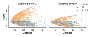
We first consider an oracle setting, where we know a priori which subsets are invariant. From our data-generating process, it follows that is the only invariant set. We then compare an invariant policy which depends only on with a policy that uses both and . We train both policies on a dataset of size obtained from multiple training environments under a fixed initial policy (see Appendix J.2). In both cases, we employ a weighted least squares to estimate the expected reward , where is the subset that the policy uses. The policy then takes a greedy action w.r.t. the estimated expected reward, i.e., (see Section 4.3). Then we evaluate both policies on multiple unseen environments and compute the regret with respect to the policy that is optimal in each of the unseen environments. Figure 2 shows the results. Each data point represents the evaluation on an unseen environment. The -axes show the regret value and the -axes display the distance from each unseen environment to the training environments (the distance is computed as the -distance between the average value of the pairs in the training environments and the pair in the unseen test environment). The plot shows that the worst-case behavior of the invariant policy is smaller than the non-invariant one. In particular, for environments different from the training environments the gain can be significant. This empirically supports our result of Theorem 1.
5.2 Learning Invariant Policies
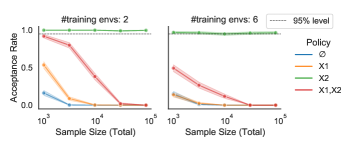
In practice, we do not know in advance which sets are invariant. We now aim to find an invariant policy from a dataset generated under an initial policy which takes both and as input. To do so, we employ the method proposed in Section 4.2 for testing invariance under distributional shifts. More precisely, we generate a dataset of size from multiple training environments under the initial policy and apply the off-policy invariance test (see Section 4.4) to verify the invariance property of each subset in . We repeat the experiment times and plot the acceptance rates at various sample sizes () (these numbers denote the total sample size, that is, number of observations, summed over all environments). The resulting acceptance rates are shown in Figure 3. Our method yields high acceptance rates for the set , which indeed is invariant, while the acceptance rates for other sets gradually decrease as the sample size increases. Furthermore, we can see that our test is more powerful when the number of training environments increases (keeping the total number of observations fixed). Our test is conservative (the acceptance rate is above the 95% level in the left plot) because the target test is not exact (the true conditional expectation is not given). In Appendix J.3, we conduct the same experiment with an exact test, using the true conditional expectation, which shows the correct level.
6 Warfarin Dosing Case Study
We evaluate our proposed approach on the clinical task of warfarin dosing. Warfarin is a blood thinner medicine prescribed to patients at risk of blood clots. The appropriate dose of warfarin varies from patient to patient depending on various factors such as demographic and genetic information (Consortium, 2009). Our case study is based on the International Warfarin Pharmacogenetics Consortium (IWPC) dataset (Consortium, 2009) which consists of patients who were treated with warfarin, collected from 21 research groups on 4 continents. The IWPC dataset contains the optimal dose of warfarin for each of the patients as well as their information on demographic characteristics, clinical and genetic factors. The warfarin dosing problem has been used in a number of previous works evaluating off-policy learning algorithms (Kallus and Zhou, 2018; Bertsimas and McCord, 2018; Zenati et al., 2020). Similarly to these works, we formulate the warfarin dosing problem as a multi-environment contextual bandit problem as follows.
-
•
The covariates are patient-level features including demographic, clinical and genetic factors.
-
•
The actions are recommended warfarin doses output by a policy. We discretize the actions into three equal-sized buckets (low, medium, high) based on the quantiles of the optimal warfarin dose.
-
•
The reward depends on the recommended dose and the optimal dose: For each patient , the reward for an action is computed as
(20) where is the optimal warfarin dose for a patient and is a median value of the optimal warfarin doses within the bucket . Here, we assume that neither the reward function nor the optimal warfarin doses are known to the agent. Instead, for each patient , only the reward for the action is observed, i.e., .
-
•
The environments are proxies for continents. The continent information is not directly contained in the dataset, but we create proxies for the continent by clustering the 21 research groups into 4 clusters based on their proportion of the patients’ race within each group. We believe that the resulting clusters roughly correspond to 4 different continents.
To reduce the search space, we select the top 10 features that are most predictive for the optimal warfarin dose using the permutation feature importance method (Breiman, 2001). The top 10 features include 4 demographic variables, 4 clinical factors, and 2 genetic factors.
We consider two experimental setups to illustrate the benefits of our invariant learning approach. In the first setup, we directly apply our method to the IWPC dataset. Here, including invariance does not seem necessary in that our method performs similarly to other baselines (but not worse). It does, however, generate some causal insight into the problem. The second setup is a semi-real setting, where we introduce an artificial, non-invariant confounder.
We now outline our first experimental setup and the results. We first generate training data by drawing actions from a policy that is constructed from linear regression of the optimal dose onto the BMI (see Appendix K.1 for more details).
6.1 Candidate Methods
Using the generated training data, we empirically compare the performance of the following policy learning methods:
-
•
Invariant Policy Learning (Inv): This is our proposed method. We first perform the off-policy invariance test using the test described in Section 4.4.3 to search for potential invariant sets. We then take the top 20 sets with the largest p-values as the candidate invariant sets. For each in , we fit the policy optimization algorithm described in Section 4.3 with as the covariates (the same algorithm is also used in other candidate methods below). Lastly, we select the top 3 sets that yield the largest expected rewards (computed using 5-fold cross-validation).
-
•
Predictive Policy Learning (Pred): This method serves as a baseline for policy learning that solely maximizes the expected reward. For each subset , we fit the policy optimization algorithm with as the covariates. We then take the policies corresponding to the top 3 sets with the largest expected rewards.
-
•
All Set Policy Learning (All): This method serves as another baseline where we take all of the patient’s features and fit the policy optimization algorithm.
6.2 Evaluation Setup & Results
We compare the policy learning methods using the following ‘leave-one-environment-out’ evaluation procedure.
-
1.
Select as a test environment. Split the training data into , where and , where .
-
2.
Using , train the policies with candidate methods detailed in Section 6.1.
-
3.
Evaluate the fitted policies by computing the expected reward on using the true reward function (20).
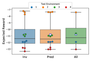
We repeat the above procedure for each and display the evaluation result in Fig 4. The performances of all candidate methods are similar. Even though the proposed invariant approach does not yield a higher reward compared with the baselines, it does not worsen the performance, either. This suggests that we can gain the stability benefit of an invariant policy without having to sacrifice predictiveness. Indeed, the stability benefit could prevent the learned invariant policy from being suboptimal when a new test environment is sufficiently different from the training environments as we show in Section 6.4
6.3 Analyzing Invariant Sets
In addition to learning an optimal invariant policy, we can use the invariance-based approach to further analyze the dependence between the patient’s features and the reward as discussed in Section 4.5. In particular, we apply the off-policy invariant causal prediction algorithm (see Algorithm 3 in Appendix G) to find potential causal ancestors of the reward. On this dataset, with a confidence level of 5%, the algorithm returns the empty set, which can happen if the covariates are highly correlated, for example Heinze-Deml et al. (2018). Nonetheless, we can still extract more information by obtaining the defining sets (see Section 2.2 in Heinze-Deml et al. (2018)). The resulting defining set of size 2 is {Race, VKORC1} (see Appendix K.2 for more details on the variables). These variables are potential causal ancestors in the sense that at least one variable in these sets is a causal ancestor.
6.4 Semi-real experiment
To further illustrate the benefits of the invariance-based learning approach, we consider a semi-real setup where we introduce hidden variables and a non-invariant predictor. We remove the two genetic factors from the patient’s features and create a non-invariant predictor that depends on those two factors as follows.
We first fit a linear regression to estimate the optimal warfarin dose from the genetic factors and denote the resulting coefficients by . To mimic environmental perturbations, we perturb depending an environment resulting in , where is an environment-specific parameter. We define the non-invariant predictor in the environment as , where are the two genetic features. We then add as part of the patient’s features and remove . The training data are generated in a similar fashion as in the first setup, except that the initial policy does not only depend on the BMI score but also on the non-invariant predictor .
In addition to the candidate methods described in Section 6.1, we introduce an additional baseline for this setup.
-
•
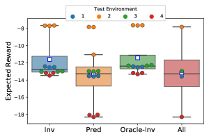
Oracle invariant Policy (Oracle-Inv): By construction, we know that is a strongly non--invariant variable (see Definition 5). This method serves as an oracle version of the invariant policy learning method by searching for the top 3 sets that do not contain such that their corresponding policies yield the largest expected reward (the procedure is similar to the Pred method with being removed).
We evaluate the candidate methods using a similar procedure as described in Section 6.2. Figure 5 illustrates the evaluation result. Our proposed method (Inv) yields a higher expected reward than the two baselines on most of the test environments. This is because the two baselines ignore the environment structure and use information from in their resulting policies, while the invariant method uses the invariance test to remove this non-invariant proxy variable. Furthermore, the performance of our proposed method is almost on par with the invariant oracle (Oracle-Inv), except for the test environment , in which our approach is unable to ignore the non-invariant predictor, possibly because the non-invariance that would be implied by Assumption 4 may not be strong enough (for our test) when .
7 Conclusion
This paper tackles the problem of environmental shifts in offline contextual bandits from a causal perspective. We introduce a framework for multi-environment contextual bandits that is based on structural causal models and frame the environmental shift problem as a distributionally robust objective over environments that are induced by different perturbations on the covariates. We prove that if there are no unobserved confounders, taking into account causality and invariance is not necessary for obtaining the distributionally robust policies. However, causality and invariance can become relevant when not all variables are observed. To tackle settings with unobserved confounders, we adapt invariance-based ideas from causal inference to the proposed framework and introduce the notion of invariant policies. Our theoretical results show that under certain assumptions an invariant policy that is optimal on the training environments is also optimal on all unseen environments, and therefore distributionally robust. We further provide a method for finding invariant policies based on an off-policy invariance test. It can be combined with any existing policy optimization algorithm to learn an optimal invariant policy. We believe that our contributions shed some light on what causality can offer in contextual bandit and, more generally, in reinforcement learning problems.
For future work, there are several directions that would be interesting to investigate. One direction is to explore the use of invariance-based ideas in the adaptive setting, in which the goal of an agent is to optimally adapt to a changing environment. Learning agents may require fewer and safer explorations in a new environment if they carry over invariance information from previous environments. It may further be possible to extend invariance-based ideas from the contextual bandit setting to the full reinforcement learning problem with long-term consequences and state dynamics. Although some previous works have explored this direction (Zhang et al., 2020; Sonar et al., 2021), we believe that the connections with respect to causality and invariance are not yet fully understood. In the i.i.d. setting, recent work has investigated trading off invariance and predictability (Rothenhäusler et al., 2021; Pfister et al., 2021; Jakobsen and Peters, 2020; Oberst et al., 2021; Saengkyongam et al., 2022). We believe that a similar idea can be applied to contextual bandit and reinforcement learning problems. Lastly, if one can gain additional knowledge of the test environments, one may aim to optimize objectives other than the worst-case performance which could lead to a different class of generalization guarantees.
This paper considers invariance as a dichotomous property and could be a first step towards using invariance-based ideas for building safer and more robust adaptive learning systems.
Acknowledgments
SS, NT, and JP were supported by a research grant (18968) from VILLUM FONDEN and JP was, in addition, supported by the Carlsberg Foundation. NP was supported by a research grant (0069071) from Novo Nordisk Fonden. We thank Steffen Lauritzen for helpful discussions.
References
- Amodei et al. (2016) D. Amodei, C. Olah, J. Steinhardt, P. Christiano, J. Schulman, and D. Mané. Concrete problems in ai safety. arXiv preprint arXiv:1606.06565, 2016.
- Arjovsky et al. (2019) M. Arjovsky, L. Bottou, I. Gulrajani, and D. Lopez-Paz. Invariant risk minimization. arXiv preprint arXiv:1907.02893, 2019.
- Athey and Wager (2021) S. Athey and S. Wager. Policy learning with observational data. Econometrica, 89(1):133–161, 2021.
- Bai et al. (2021) T. Bai, J. Luo, J. Zhao, B. Wen, and Q. Wang. Recent advances in adversarial training for adversarial robustness. In Proceedings of the Thirtieth International Joint Conference on Artificial Intelligence, IJCAI-21, 2021. Survey Track.
- Bareinboim and Pearl (2014) E. Bareinboim and J. Pearl. Transportability from multiple environments with limited experiments: Completeness results. Advances in neural information processing systems, 27, 2014.
- Bareinboim and Pearl (2016) E. Bareinboim and J. Pearl. Causal inference and the data-fusion problem. Proceedings of the National Academy of Sciences, 113(27):7345–7352, 2016.
- Bareinboim et al. (2015) E. Bareinboim, A. Forney, and J. Pearl. Bandits with unobserved confounders: A causal approach. Advances in Neural Information Processing Systems, 28, 2015.
- Bertsimas and McCord (2018) D. Bertsimas and C. McCord. Optimization over continuous and multi-dimensional decisions with observational data. In Advances in Neural Information Processing Systems, volume 31. Curran Associates, Inc., 2018.
- Beygelzimer and Langford (2009) A. Beygelzimer and J. Langford. The offset tree for learning with partial labels. In Proceedings of the 15th ACM SIGKDD International Conference on Knowledge Discovery and Data Mining, pages 129–138, 2009.
- Bongers et al. (2016) S. Bongers, P. Forré, J. Peters, and J. M. Mooij. Foundations of structural causal models with cycles and latent variables. The Annals of Statistics (accepted), arXiv preprint arXiv:1611.06221, 2016.
- Bottou et al. (2013) L. Bottou, J. Peters, J. Quiñonero-Candela, D. X. Charles, D. M. Chickering, E. Portugaly, D. Ray, P. Simard, and E. Snelson. Counterfactual reasoning and learning systems: The example of computational advertising. Journal of Machine Learning Research, 14(65):3207–3260, 2013.
- Breiman (2001) L. Breiman. Random forests. Machine learning, 45(1):5–32, 2001.
- Christiansen et al. (2021) R. Christiansen, N. Pfister, M. E. Jakobsen, N. Gnecco, and J. Peters. A causal framework for distribution generalization. IEEE Transactions on Pattern Analysis and Machine Intelligence, pages 1–1, 2021. doi: 10.1109/TPAMI.2021.3094760.
- Consortium (2009) I. W. P. Consortium. Estimation of the warfarin dose with clinical and pharmacogenetic data. New England Journal of Medicine, 360(8):753–764, 2009.
- Correa and Bareinboim (2020) J. Correa and E. Bareinboim. General transportability of soft interventions: Completeness results. Advances in Neural Information Processing Systems, 33:10902–10912, 2020.
- Dawid (2002) A. P. Dawid. Influence diagrams for causal modelling and inference. International Statistical Review, 70(2):161–189, 2002.
- de Kroon et al. (2020) A. A. de Kroon, D. Belgrave, and J. M. Mooij. Causal discovery for causal bandits utilizing separating sets. arXiv preprint arXiv:2009.07916, 2020.
- Dudik et al. (2011) M. Dudik, J. Langford, and L. Li. Doubly robust policy evaluation and learning. In Proceedings of the 28th International Conference on Machine Learning, pages 1097–1104. ACM, 2011.
- Dunn (1961) O. J. Dunn. Multiple comparisons among means. Journal of the American Statistical Association, 56(293):52–64, 1961.
- Garcıa and Fernández (2015) J. Garcıa and F. Fernández. A comprehensive survey on safe reinforcement learning. Journal of Machine Learning Research, 16(1):1437–1480, 2015.
- Glymour et al. (2019) C. Glymour, K. Zhang, and P. Spirtes. Review of causal discovery methods based on graphical models. Frontiers in genetics, 10:524, 2019.
- Gretton et al. (2012) A. Gretton, K. M. Borgwardt, M. J. Rasch, B. Schölkopf, and A. Smola. A kernel two-sample test. Journal of Machine Learning Research, 13(25):723–773, 2012.
- Guestrin et al. (2002) C. Guestrin, D. Koller, and R. Parr. Multiagent planning with factored MDPs. In T. Dietterich, S. Becker, and Z. Ghahramani, editors, Advances in Neural Information Processing Systems, volume 14. MIT Press, 2002.
- Guestrin et al. (2003) C. Guestrin, D. Koller, R. Parr, and S. Venkataraman. Efficient solution algorithms for factored MDPs. J. Artif. Int. Res., 19(1):399–468, 2003.
- Heinze-Deml et al. (2018) C. Heinze-Deml, J. Peters, and N. Meinshausen. Invariant causal prediction for nonlinear models. Journal of Causal Inference, 6(2):1–35, 2018.
- Jakobsen and Peters (2020) M. E. Jakobsen and J. Peters. Distributional robustness of k-class estimators and the pulse. arXiv preprint arXiv:2005.03353, 2020.
- Jonsson and Barto (2006) A. Jonsson and A. Barto. Causal graph based decomposition of factored MDPs. Journal of Machine Learning Research, 7(81):2259–2301, 2006.
- Jung et al. (2020a) Y. Jung, J. Tian, and E. Bareinboim. Estimating causal effects using weighting-based estimators. Proceedings of the AAAI Conference on Artificial Intelligence, 34, 2020a.
- Jung et al. (2020b) Y. Jung, J. Tian, and E. Bareinboim. Learning causal effects via weighted empirical risk minimization. In Advances in Neural Information Processing Systems, volume 33. Curran Associates, Inc., 2020b.
- Kallus (2018) N. Kallus. Balanced policy evaluation and learning. In Advances in Neural Information Processing Systems, volume 31. Curran Associates, Inc., 2018.
- Kallus and Zhou (2018) N. Kallus and A. Zhou. Policy evaluation and optimization with continuous treatments. In International Conference on Artificial Intelligence and Statistics, pages 1243–1251. PMLR, 2018.
- Kallus and Zhou (2020) N. Kallus and A. Zhou. Confounding-robust policy evaluation in infinite-horizon reinforcement learning. Advances in Neural Information Processing Systems, 33:22293–22304, 2020.
- Kearns and Koller (1999) M. Kearns and D. Koller. Efficient reinforcement learning in factored MDPs. In Proceedings of the 16th International Joint Conference on Artificial Intelligence, page 740–747. Morgan Kaufmann Publishers Inc., 1999.
- Kruskal and Wallis (1952) W. H. Kruskal and W. A. Wallis. Use of ranks in one-criterion variance analysis. Journal of the American statistical Association, 47(260):583–621, 1952.
- Langford and Zhang (2008) J. Langford and T. Zhang. The epoch-greedy algorithm for multi-armed bandits with side information. In Advances in Neural Information Processing Systems, volume 20. Curran Associates, Inc., 2008.
- Lattimore et al. (2016) F. Lattimore, T. Lattimore, and M. D. Reid. Causal bandits: Learning good interventions via causal inference. In Advances in Neural Information Processing Systems, volume 29. Curran Associates, Inc., 2016.
- Lauritzen et al. (1990) S. L. Lauritzen, A. P. Dawid, B. N. Larsen, and H.-G. Leimer. Independence properties of directed Markov fields. Networks, 20:491–505, 1990.
- Lee and Bareinboim (2018) S. Lee and E. Bareinboim. Structural causal bandits: Where to intervene? In Advances in Neural Information Processing Systems, volume 31. Curran Associates, Inc., 2018.
- Lee et al. (2020) S. Lee, J. D. Correa, and E. Bareinboim. Generalized transportability: Synthesis of experiments from heterogeneous domains. In Proceedings of the 34th AAAI Conference on Artificial Intelligence, 2020.
- Magliacane et al. (2018) S. Magliacane, T. van Ommen, T. Claassen, S. Bongers, P. Versteeg, and J. M. Mooij. Domain adaptation by using causal inference to predict invariant conditional distributions. In Advances in Neural Information Processing Systems, volume 31. Curran Associates, Inc., 2018.
- Meek (1995) C. Meek. Strong completeness and faithfulness in bayesian networks. In Proceedings of the Eleventh Conference on Uncertainty in Artificial Intelligence, UAI’95, 1995.
- Muandet et al. (2013) K. Muandet, D. Balduzzi, and B. Schölkopf. Domain generalization via invariant feature representation. In Proceedings of the 30th International Conference on Machine Learning, pages 10–18. PMLR, 2013.
- Newey and McFadden (1994) W. K. Newey and D. McFadden. Chapter 36 large sample estimation and hypothesis testing. volume 4 of Handbook of Econometrics, pages 2111–2245. Elsevier, 1994. doi: https://doi.org/10.1016/S1573-4412(05)80005-4.
- Oberst et al. (2021) M. Oberst, N. Thams, J. Peters, and D. Sontag. Regularizing towards causal invariance: Linear models with proxies. In International Conference on Machine Learning, pages 8260–8270. PMLR, 2021.
- Pearl (1995) J. Pearl. Causal diagrams for empirical research. Biometrika, 82(4):669–688, 1995.
- Pearl (2009) J. Pearl. Causality. Cambridge University Press, 2009.
- Pearl (2016) J. Pearl. Causal inference in statistics : a primer. Wiley, 2016.
- Pearl and Bareinboim (2011) J. Pearl and E. Bareinboim. Transportability of causal and statistical relations: A formal approach. In Twenty-fifth AAAI conference on artificial intelligence, 2011.
- Peters et al. (2016) J. Peters, P. Bühlmann, and N. Meinshausen. Causal inference using invariant prediction: identification and confidence intervals. Journal of the Royal Statistical Society, Series B (Statistical Methodology) (with discussion), 78, 2016.
- Peters et al. (2017) J. Peters, D. Janzing, and B. Schölkopf. Elements of causal inference: foundations and learning algorithms. The MIT Press, 2017.
- Pfister et al. (2018) N. Pfister, P. Bühlmann, and J. Peters. Invariant causal prediction for sequential data. Journal of the American Statistical Association, 114(527):1264–1276, 2018.
- Pfister et al. (2019) N. Pfister, S. Bauer, and J. Peters. Learning stable and predictive structures in kinetic systems. Proceedings of the National Academy of Sciences, 116(51):25405–25411, 2019.
- Pfister et al. (2021) N. Pfister, E. G. Williams, J. Peters, R. Aebersold, and P. Bühlmann. Stabilizing variable selection and regression. Annals of Applied Statistics (accepted), 2021.
- Rojas-Carulla et al. (2018a) M. Rojas-Carulla, B. Schölkopf, R. Turner, and J. Peters. Causal transfer in machine learning. Journal of Machine Learning Research, 19(36):1–34, 2018a.
- Rojas-Carulla et al. (2018b) M. Rojas-Carulla, B. Schölkopf, R. Turner, and J. Peters. Invariant models for causal transfer learning. The Journal of Machine Learning Research, 19:1309–1342, 2018b.
- Rothenhäusler et al. (2021) D. Rothenhäusler, N. Meinshausen, P. Bühlmann, and J. Peters. Anchor regression: Heterogeneous data meet causality. Journal of the Royal Statistical Society: Series B (Statistical Methodology), 83(2):215–246, 2021.
- Saengkyongam et al. (2022) S. Saengkyongam, L. Henckel, N. Pfister, and J. Peters. Exploiting independent instruments: Identification and distribution generalization. arXiv preprint arXiv:2202.01864, 2022.
- Schölkopf et al. (2012) B. Schölkopf, D. Janzing, J. Peters, E. Sgouritsa, K. Zhang, and J. M. Mooij. On causal and anticausal learning. In Proceedings of the 29th International Conference on Machine Learning, pages 1255–1262. Omnipress, 2012.
- Sen et al. (2017) R. Sen, K. Shanmugam, M. Kocaoglu, A. Dimakis, and S. Shakkottai. Contextual bandits with latent confounders: An nmf approach. In Artificial Intelligence and Statistics, pages 518–527. PMLR, 2017.
- Sonar et al. (2021) A. Sonar, V. Pacelli, and A. Majumdar. Invariant policy optimization: Towards stronger generalization in reinforcement learning. In Learning for Dynamics and Control, pages 21–33. PMLR, 2021.
- Spirtes et al. (2000) P. Spirtes, C. Glymour, and R. Scheines. Causation, Prediction, and Search. MIT Press, 2nd edition, 2000.
- Strehl et al. (2010) A. Strehl, J. Langford, L. Li, and S. M. Kakade. Learning from logged implicit exploration data. In Advances in Neural Information Processing Systems, volume 23. Curran Associates, Inc., 2010.
- Subbaswamy et al. (2019) A. Subbaswamy, P. Schulam, and S. Saria. Preventing failures due to dataset shift: Learning predictive models that transport. In The 22nd International Conference on Artificial Intelligence and Statistics, pages 3118–3127. PMLR, 2019.
- Sugiyama and Kawanabe (2012) M. Sugiyama and M. Kawanabe. Machine learning in non-stationary environments: Introduction to covariate shift adaptation. MIT press, 2012.
- Swaminathan and Joachims (2015a) A. Swaminathan and T. Joachims. Counterfactual risk minimization: Learning from logged bandit feedback. In Proceedings of the 32nd International Conference on Machine Learning, pages 814–823. PMLR, 2015a.
- Swaminathan and Joachims (2015b) A. Swaminathan and T. Joachims. The self-normalized estimator for counterfactual learning. In Advances in Neural Information Processing Systems, volume 28, pages 3231–3239. Curran Associates, Inc., 2015b.
- Tennenholtz et al. (2020) G. Tennenholtz, U. Shalit, and S. Mannor. Off-policy evaluation in partially observable environments. In Proceedings of the AAAI Conference on Artificial Intelligence, volume 34, pages 10276–10283, 2020.
- Tennenholtz et al. (2021) G. Tennenholtz, U. Shalit, S. Mannor, and Y. Efroni. Bandits with partially observable confounded data. In Uncertainty in Artificial Intelligence, pages 430–439. PMLR, 2021.
- Thams et al. (2021) N. Thams, S. Saengkyongam, N. Pfister, and J. Peters. Statistical testing under distributional shifts. arXiv preprint arXiv:2105.10821, 2021.
- Tian et al. (1998) J. Tian, A. Paz, and J. Pearl. Finding minimal d-separators. Technical report, University of California, Los Angeles, 1998.
- Tibshirani (1996) R. Tibshirani. Regression shrinkage and selection via the lasso. Journal of the Royal Statistical Society: Series B (Methodological), 58(1):267–288, 1996.
- Volpi et al. (2018) R. Volpi, H. Namkoong, O. Sener, J. C. Duchi, V. Murino, and S. Savarese. Generalizing to unseen domains via adversarial data augmentation. In Advances in Neural Information Processing Systems, volume 31. Curran Associates, Inc., 2018.
- Yabe et al. (2018) A. Yabe, D. Hatano, H. Sumita, S. Ito, N. Kakimura, T. Fukunaga, and K.-i. Kawarabayashi. Causal bandits with propagating inference. In Proceedings of the 35th International Conference on Machine Learning, volume 80, pages 5512–5520. PMLR, 2018.
- Ye et al. (2021) H. Ye, C. Xie, T. Cai, R. Li, Z. Li, and L. Wang. Towards a theoretical framework of out-of-distribution generalization. Advances in Neural Information Processing Systems, 34, 2021.
- Zenati et al. (2020) H. Zenati, A. Bietti, M. Martin, E. Diemert, and J. Mairal. Counterfactual learning of continuous stochastic policies. arXiv preprint arXiv:2004.11722, 2020.
- Zhang et al. (2020) A. Zhang, C. Lyle, S. Sodhani, A. Filos, M. Kwiatkowska, J. Pineau, Y. Gal, and D. Precup. Invariant causal prediction for block MDPs. In Proceedings of the 37th International Conference on Machine Learning, volume 119, pages 11214–11224. PMLR, 2020.
- Zhang (2004) T. Zhang. Solving large scale linear prediction problems using stochastic gradient descent algorithms. In Proceedings of the 21st International Conference on Machine Learning, page 116, 2004.
- Zhou et al. (2022) Z. Zhou, S. Athey, and S. Wager. Offline multi-action policy learning: Generalization and optimization. Operations Research, 2022.
Appendix A Pearl’s -separation
Definition 6 (Pearl’s -separation (Pearl, 2009; Peters et al., 2017)).
Let be directed acyclic graph (DAG) with nodes . Let and . A path between nodes and is said to be blocked by a set if there exists a node such that one of the following holds:
-
1.
and
or or -
2.
neither nor any of its descendants is in and
For any three disjoint subsets of nodes in , we say that and are -separated by , denoted by if every path between nodes in and is blocked by .
(This formulation is taken from Peters et al. (2017).)
Appendix B Policy Learning without Unexplained Environment Shifts
This section presents an assumption under which it is not beneficial to explicitly take into account the environment structure. In particular, simply pooling the data from all training environments and applying a standard value-based policy learning algorithm yields a solution to (4). This result sheds light on the role of causality and invariance in contextual bandits and reinforcement learning. The relevant assumption is the following.
Assumption 5.
Assume that .
In words, under Assumption 5, the influence of the environment on the reward can be fully explained by the observed covariates . This assumption holds, for example, if there are no hidden confounders between and that are directly affected by .
The following proposition shows that under Assumption 5 there is a population optimal policy that does not depend on the environments. In particular, this optimal policy can be learned from data obtained in any observed subset of the environments .
Proposition 5.
Proof.
See Appendix D.1. ∎
This type of generalization is well-established in the context of regression. In the contextual bandit setting the value function changes across environments, so instead one needs to use that the Q-function does not change across environments and then argue that this implies that the optimal policy remains the same in each environment. Proposition 5 suggests that we can estimate an optimal policy by pooling the data from training environments and applying a standard value-based policy learning algorithm. This is indeed the case.
Let be an estimator of the conditional mean that is based on independent observations from potentially different environments. The following proposition shows that such an approach indeed yields a consistent estimate of an optimal policy given that is consistent.
Proposition 6.
Assume Setting 1 and Assumption 5. Let be a uniformly consistent estimator of , that is, for all it holds that
where is an expectation over the observations used to estimate . Let be any policy that maximizes , i.e., for all and all it holds that
Then, the robust policy value converges towards its optimal value, that is
Proof.
See Appendix D.2. ∎
The same argument would work if instead of pooling, one considers only a single environment. In practice, however, one would make use of all available data. Whether it is possible to construct a uniformly consistent estimator depends on the model class that can be assumed in the structural assignment of , and on the policy used in generating the observations. For example, in the case of additive confounding and noise such as with and in some function classes and a policy that has full support, (i.e., ), one can consider a least squares estimator of the form
The assumptions of Proposition 6 are then satisfied under further constraints on the function class and noise distributions, e.g., linear functions, Gaussian noise, and bounded domains.
Appendix C Backdoor Adjustment and Reweighting Approaches
In our work, we take a reweighting approach for estimating the causal estimand (as presented in Section 4.3) as opposed to using the backdoor adjustment formula. We have decided to use the reweighting approach for several reasons.
-
(i)
To test the -invariance hypothesis, the reweighting approach allows us to use the resampling procedure (Thams et al., 2021) that allows to apply arbitrary invariance tests while perserving pointwise asymptotic level. In contrast, it is not immediate how one can develop an asymptotically valid test based directly on the formula given by the backdoor adjustment.
- (ii)
It has been shown in Jung et al. (2020b) that the two formulations imply equivalent identification results for causal effects. More specifically, any causal effect that is identified by do-calculus (Pearl, 1995) (e.g., by the backdoor adjustment formula) can also be identified via empirical risk minimization in a reweighted distribution. For completeness, we make this connection explicit for the setting considered in this work.
Consider the observed variables in Setting 1 with a fixed initial policy in a fixed environment . For notational convenience, we denote the density simply by and assume, without affecting the generality of the result, that all the variables are discrete. Fix and define as the complement of . We are interested in the causal quantity or equivalently, using do-notation, . (Note that the causal quantity is the same for any ). Since the graph in Setting 1 satisfies (i) -variables are non-descendants of and (ii) , we have that satisfies the backdoor criterion and hence the causal quantity is identifiable via the adjustment formula (see (Pearl, 2016, Section 3.5))
| (22) |
We will now show that can also be expressed in terms of a reweighted distribution. To this end, we define a weighting factor , and define a target distribution . The following statements hold.
-
•
Using an appropriate factorization, we get
(23) -
•
From (23), we have
(24) -
•
From (23), we have
(25) - •
- •
Now, we show that the backdoor adjustment formula for , given in (22), can be expressed in terms of a conditional density in the target distribution as follows
| by (22) | ||||
| by (26) | ||||
| by (25) | ||||
| by (27) | ||||
Appendix D Proofs
D.1 Proof of Proposition 5
Proof.
Let , and be arbitrary. By the Markov property (see Lemma 3) we have that does not depend on the environment. This, in particular, implies that for all , all and all , it holds that
| (28) |
We thus have for all policies and for all that
| (29) |
Next, take the expectation over on both sides to get
Finally, taking the infimum over leads to
| (30) |
Let be a policy such that for all and all
| (31) |
Then satisfies, for all ,
Therefore (30) implies
which completes the proof of Proposition 5. ∎
D.2 Proof of Proposition 6
Proof.
Define for all the term
As is assumed to be finite and because is assumed to be uniformly consistent, it holds that
| (32) |
Moreover, as shown in (28), in the proof of Proposition 5, we know that for all , all and all it holds that
This implies that for all and all it holds that
| (33) |
Each of the sums only contains one terms, since puts all mass on a single action. Next, observe that
| (34) |
and
| (35) | |||
Using (33), (34) and (35) together with the triangle inequality yields
This in particular implies that for all and all it holds that
and that
Taking the expectation over and the infimum over in both inequalities leads to
where is the policy defined in (21). Finally, we use (32) and Proposition 5 to get that
This completes the proof of Proposition 6. ∎
D.3 Proof of Lemma 1
The key argument in the proof of Lemma 1 is a Markov property that we formulate as a lemma below.
Lemma 3 (Extended Markov Property).
Assume Setting 1. For all subsets , it holds for all that
where the symbol denotes d-separation in the graph .
Proof.
D.3.1 Proof of Lemma 3
Proof.
Lemma 3 corresponds to a global Markov property in the augmented graph (including the non-random environment index). Such results are well-established and used in settings in which is finite, for example in influence diagrams (Dawid, 2002). The result, however, also holds for more general, even uncountable .
To prove this, we first fix , and . Furthermore, let , let be the discrete -algebra on and let be a probability measure that puts non-zero mass on . We can then replace the environment indicator in the SCM with a random variable with distribution . This induces a joint distribution over that is globally Markov with respect to the graph , where is now replaced by (see Pearl (2009) Thm 1.4.1 or Lauritzen et al. (1990)). Additionally, it satisfies that has the same distribution as the distribution induced by . Therefore the d-separation (which is implied by ) implies that the joint distribution satisfies the following conditional independence
| (36) |
Next, denote by the density of with respect to a product measure with the discrete measure as the -component and for all denote by the induced density of . Then, by construction of the densities and using the conditional independence in (36) it holds that for all , all and all with that
The function therefore no longer depends on the environment nor on . Since , this in particular implies that for all and all it holds that
As this construction works for all , this completes the proof of Lemma 3. ∎
D.4 Stable Blanket and Invariance
In this section, if not explicitly stated otherwise, all causal relations such as parents, descendants, ancestors etc. refer to the graph . Moreover, we use the convention that , where denotes only the -variable descendants of . We first define the strongly non--invariant set:
where CI are confounded and directly intervened on nodes (i.e., for there exists such that in ) and define . Furthermore, we define to be the set of -variables such that if and only if in or there is a directed path in , where consists of -variables. The following Lemma will serve as a basis for our proofs of Proposition 1 and Theorem 1.
Lemma 4 (properties of ).
Proof.
The proof is divided into four parts (S.1, S.2, S.3 and S.4):
-
S.1
We prove that if then by contraposition. Let be a subset such that there exists but . This implies that there exist and such that in and . Since , the path is open given , and therefore . By Definition 3, this implies that is not -invariant, leading to a contradiction.
-
S.2
In this step, we prove that if a -invariant set exists, it holds that . We prove this by contraposition. Assume that there exists such that . This implies that there exist and such that in and . Now, we construct a contradiction by showing that this would imply that no -invariant set exists. Let be an arbitrary set. There are two possibilities,
-
(a)
: Using the same argument as in S.1, we have that is not a -invariant set.
-
(b)
: Since but there exists a directed path (using that )
where part 2 either has length zero or consists only of -variables (by definition of ). The only way this path can be blocked by is if either , or one of the variables in part 1 are contained in . However, if this is the case the path is open given . Since the edges from to are not relevant in this case, this in particular means that , which by Definition 3 implies that is not -invariant.
As these are the only two possibilities, we have shown that no -invariant set exists, which is a contradiction. Therefore .
-
(a)
-
S.3
Now we prove that if a -invariant set exists, then is -invariant. In this step, all the graphical statements are understood to be taken in . Let be an arbitrary path from to in . We first consider the two trivial cases. (i) enters through , i.e., that it has the form
By construction of this path can only be in if which implies that it is blocked by . (ii) enters directly from -variables. Let be the -variable on that is closest to , then has the form . By Assumption 2, there must be an edge from to and hence simplifies to . Because is unobserved, any set would then not be -invariant which contradicts to the assumption that there is a -invariant set. Next we consider more involved cases, assume that enters either through a - or -variable. Let be the -variable on that is closest to and be the -variable on that is closest to . We consider the two following cases:
-
(1)
does not exist: This implies that does not contain any unobserved variables and hence can enter only through an X-variable. By S.2, we have and hence it holds that is blocked by .
-
(2)
exists: has the form
where part 1 could be of length zero or it could consist of further -variables and part 2 could be of length zero or it could consist of further -or -variables. By Assumption 2, we have that there must be an edge from to and hence there exists another path
where part 1 corresponds to the part 1 from path . It suffices to show that is blocked by : whenever is blocked by , is blocked by too (as . We now consider the following three cases for :
-
(i)
,
-
(ii)
,
-
(iii)
,
in each case the can also be of length zero.
Case (i): We show by contradiction that is blocked by . Assume is open given , i.e., . Let be an arbitrary subset. If , then by the definition of there exists and such that in and and hence . If , then the path is open given and hence . Therefore, there is no -invariant set which contradicts to the fact that a -invariant set exists.
Case (ii): In this case, is a collider on . Assume has the form . This implies that and hence is blocked by . Thus, in order for to be open given it must have the form . Now, we consider the following two cases separately:-
(a)
: This directly implies that is blocked by .
-
(b)
: By definition of it holds that . Hence, also which since is a collider implies that is blocked by .
We have therefore shown that in Case (ii) the path is blocked by .
Case (iii): In this case, let be the collider closest to on . Again we consider two cases:-
(a)
: This directly implies that is blocked by .
-
(b)
: Since , this implies that . Hence, the path is blocked by .
We have therefore shown that in Case (iii) the path is blocked by . Combining all cases, we have shown that any path from to is blocked by in .
-
(i)
-
(1)
-
S.4
It remains to show that
We show each direction separately. First, let . By the definition of it holds that there exists and such that in and . As this path does not involve it is contained in for all subsets . Moreover, since is a collider and the only -variable on this path, it holds that this path will be open given for all subsets . Therefore, is strongly non--invariant. Next, to show the reverse direction let . Then, by S.3 it holds that is -invariant. So in particular , which since implies that is not strongly non--invariant.
This completes the proof of Lemma 4. ∎
As shown in Lemma 4 the set is -invariant and contains all -invariant sets if a -invariant set exists. It will be used in the proofs of Proposition 1 and Theorem 1 to find the optimal -invariant policy, as it encodes all invariant available information about the reward. The set is related to stable blankets as defined in Pfister et al. (2021).
D.5 Proof of Proposition 1
Proof.
As before, we define as the policy that always selects the action . We first show an intermediate result and then turn to the proof of Proposition 1.
Lemma 5.
Let be an invariant set. It holds for all that
| (37) |
Proof.
Let be a -invariant set and be an environment. By the same arguments as in (29) we have, for all , it holds that
where we drop the environment in the expectations as is -invariant (see Lemma 1). Taking the expectation over on both sides yields
| (38) |
Let be a policy that satisfies for all and for -a.e.
| (39) |
We have that
By (38), we then have that . We now show the reverse direction, i.e., if , then satisfies (39).
Now we prove the first statement of Proposition 1. To this end, let
By Lemma 5, we have for all that
So in particular, for all , it holds that
Thus it holds for all , all and all that
Taking the infimum over on both sides yields
Because this inequality holds for all and all , this implies
| (42) |
This completes the proof of Proposition 1(i).
Next we prove the second statement of Proposition 1. The proof arguments are largely similar to those of the first statement except here we make use of the set defined in Section D.4 which is a superset of all other -invariant sets. The proof is divided into two steps (S.1, S.2)
- S.1
-
S.2
In the second step, we are now ready to prove the main result of the statement. To this end, let
Since (44) holds for all , we have for all that
Then, By Lemma 5 we have for all that
So in particular, for all , it holds that
Thus it holds for all , all and all that
Taking the infimum over on both sides yields
Because this inequality holds for all and all , this implies
(45) This completes the proof of Proposition 1(ii).
∎
D.6 Proof of Theorem 1
Proof.
We first prove the first statement of Theorem 1. Fix a policy
Using the same argument as we made in Section D.5(S.3), we get that for all it holds that
| (46) |
Hence by Jensen’s inequality it holds that
This completes the proof of the first statement.
Next, we prove the second statement of Theorem 1. To do so, we use the following lemma, which is proved in Section D.6.1 below.
Lemma 6 (Upper bound).
D.6.1 Proof of Lemma 6
Proof.
Recall the terminology and notation from Section D.4. The proof can be split into two parts:
-
1.
We first prove that if is a confounding removing environment it holds for all that
(49) -
2.
We then prove the upper bound using step 1) as the main argument.
Step 1) Let be a confounding removing environment and fix and . By Lemma 4 it holds that is strongly non--invariant. Therefore, since is a confounding removing environment, we get that
| (50) |
Now, let be an arbitrary path from to in . We consider the following (separate) cases that can occur:
-
(a)
enters through : Then the path is blocked by and because is not a collider and hence blocks .
-
(b)
only contains and -variables and enter through -variables: Then there exists such that ends with . This implies that since is a sub-graph of . Furthermore, since by Lemma 4 (recall that ) , this implies that . Hence, is blocked by and because is not a collider.
-
(c)
contains at least one -variable: Let such that is the -variable closest to on , i.e., has the form
Now, by (50) it holds that is blocked (given the empty set) in and by construction it only consists of -variables (except ). Therefore, there must be at least one collider on . Let be the collider closest to and let (this could be ) the variable that comes right before on , i.e.,
We consider two cases:
-
(i)
First, assume that (in ), then it holds, by the definition of and since is a subgraph of , that as well (otherwise none of the descendants of could be in as ). However, is not a collider and therefore is blocked given and .
-
(ii)
Second, assume , then it in particular holds that which by Lemma 4 implies that is strongly non--invariant. Hence, because is a confounding removing environment, it holds that . However, was selected to be the collider closest to which means that the part of from to is open in leading to a contradiction.
-
(i)
We have therefore shown that the path is always blocked given and . Since was arbitrary this implies that .
Step 2)
Now, we are ready to prove the main result. Let be an arbitrary non--invariant policy, and let such that . We have
| by the tower property of conditional expectation, | ||||
Now, we use Assumption 3. For each we choose a confounding removing environment such that . Because the confounding removing environments are a subset of , we have
| Using that , we then have | ||||
Next, we use (49) which states that for all it holds that . Then, by the Markov property, we get
| we can then omit since is a -invariant set (by Lemma 4 since ), | ||||
| letting , | ||||
∎
D.7 Proof of Lemma 2
Proof.
Let be an initial policy generating the training data. For each and , we have that
We therefore have for all and that
∎
D.8 Proof of Proposition 3
Proof.
Fix , let be the uniform random policy given for all and all by
and define . First, we rewrite the objective function in (16) in terms of as follows
We now show that (a) is uniquely minimized at and (b) satisfies the weak uniform law of large numbers. Then, together with (i) and (iii), Theorem 2.1 in Newey and McFadden (1994) implies that in probability as desired.
First, we show (a). Taking the expectation, we have
| (51) |
Next, let be any observed environment, it holds for all and for -a.e. that
| (52) |
where holds because is -invariant, and holds by (ii). Now, since the conditional mean is the (almost surely) unique minimizer of
(52) implies that . Furthermore, using that
we get that
Hence, we have shown (a).
Next, we show (b), that is, the objective function satisfies the weak uniform law of large numbers. By (v) and (iv) we have for all that . Furthermore, define , then by Lemma 2.4 in Newey and McFadden (1994) it holds for all that in probability as and hence that in probability as , which proves (b).
D.9 Proof of Proposition 2
D.10 Proof of Proposition 4
Proof.
Let be the set of observed ancestors of . In this proof, all the graphical statements are understood to be taken in . Assume that a -invariant set exists. Then, by Theorem 2 of Tian et al. (1998), is -invariant, too (indeed, intersected with all ancestors of is -invariant but as does not contain any hidden variables, this set equals ).
Appendix E Connection to Random Environments
It is possible to define multi-environment contextual bandits using random environments.
Setting 2 (Random Environment Contextual Bandits).
Let , , , , . For any , let denote the function that ensures, for all , equals in distribution for a uniformly distributed . Now, consider functions , , and , a factorizing distribution whose component is uniform, and a structural causal model given by
Assume further that for all , the SCM induces a unique distribution over , which we denote by . The structure of the SCM can be also visualized by a graph which is constructed in a similar way to the graph in Setting 1, except that the environment becomes one of the variable nodes in this graph.
Appendix F Details for Section 4.2
In Section 4.2, we propose to use the resampling procedure in Thams et al. (2021) to test the hypothesis of invariance under a test policy .
For every , we have a dataset consisting of observations is available.111111It is possible to allow for a different initial policy at each observation . One then needs to define the relative weights . For all and all define the relative weights as
| (53) |
Then, for all , we draw a weighted resample of size from with weights
| (54) |
We then apply an invariance test to the resampled data . A family of invariance tests is a collection of functions such that for each , is a function (into ) that takes data from environments , each of size , and tests whether is invariant. Here, indicates that we reject the hypothesis of invariance. We say the test has pointwise asymptotic level if for all invariant sets and all it holds that
We state that the overall procedure (resampling and then testing) has asymptotic level as long as the test has asymptotic level. For simplicity, we assume that and . The following result follows directly from (Thams et al., 2021, Theorem 1)
Proposition 7.
Let and suppose that for each environment , we observe a dataset consisting of observations . Consider and assume that for all , , where is defined in (53). Let and for all , let be a resample of drawn with weights given by (54). Let be a hypothesis test for invariance of the conditional expectation that has pointwise asymptotic level when is applied to data sampled with . Applying to the resampled data yields pointwise asymptotic level, that is,
if is invariant.
Proof.
We only show that this problem with environments can be cast in the setting of Thams et al. (2021), which has no reference to environments. Here, we assume that we have the same number of observations in each environment. The main idea is to create a dataset , such that each observation in consists of an observation from each of the environments .
First, we randomly permute the observations within each dataset to obtain a set . Then, we construct an auxiliary dataset , where the ’th observation of is the concatenation of the ’th observation (after permutation) from each of the environments, .
We can now apply the resampling methodology from Thams et al. (2021) to draw a sequence with weights given by
where
and are the ’th observation of . Because the observations are independent, both within and between environments, the probability of drawing the sample is equal to the probability of drawing first observations from , , and then from etc. The result then follows directly from Thams et al. (2021). ∎
In other words, we can test whether is invariant by resampling the data and applying an invariance test on the resampled dataset. Proposition 7 states that this procedure holds level asymptotically. We assume knowledge of the initial policy to ease our presentation. We can, in fact, show the pointwise asymptotic validity even if the initial policy is unknown and has to be estimated from the offline data (see Thams et al. (2021) Theorem 2).
Appendix G Algorithm: Off-policy Invariant Causal Prediction
Below, we present an algorithm for finding the causal ancestors of the reward under a change in policy.
Appendix H Faster power optimization
In Section 4.4.2, we show that we can optimize the power to detect non-invarince by gradient descent. In particular, the gradient is
where is a resample of the data and pv is a function returning a p-value of our invariance test. is given by Equation (54), but as discussed in Thams et al. (2021), this may be infeasible to compute if is very large.
As a computationally efficient alternative, Thams et al. (2021) proposes an approximate resampling scheme, where a sequence (distinct or non-distinct) is sampled with replacement. That is, the weights are given by
This expression is much easier to compute than Equation (54), because the denominator is a sum over terms (instead of ). In particular, we get
Algorithm 4 splits the data in two halves: we optimize power on the first half of the data and test for invariance on the second half. We only use the above approximation for the power optimization, where we need to explicitly compute the normalization constant of the weights. In the second half of Algorithm 4, we use Equation (54) (i.e., we do not use the approximate weights), because Proposition 7 requires the weights to be those given in Equation (54). If is so large that we cannot sample by explicitly computing the weights Equation (54), there are several options for sampling from the scheme without computing the denominator – see Thams et al. (2021) for a variety of approaches.
Appendix I Invariance test with optimized test policy
In this section we provide Algorithm 4, which tests the invariance of a set by choosing a test policy that optimizes the power of the invariance test, as discussed in Section 4.4.2.
Appendix J Simulation Details
J.1 Data Generating Process
We generate data from the following SCM :
where , takes values in the space . In our experiments, we consider and randomly draw the parameters from , while the environment-specific parameters are drawn from . These parameters are then fixed across all experiment runs.
J.2 Initial Policy
We construct an initial policy in Section 5 as follows. First, we generate a training data from the uniform random policy and partition the dataset according to the action values: , …, . Then, for each action , we fit a linear regression on to estimate the reward from and . Denote the resulting regressor as . The initial policy is then constructed as
J.3 Invariant Test with True Conditional Expectation
This section contains Figure 6, in which we display acceptance rates for the same experiment as in Section 5.2 but with an exact test, using the true conditional expectation. The figure suggests that the procedure indeed holds level.
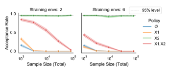
Appendix K Warfarin Case Study
K.1 Initial Policy
We generate the training data , where under the following initial policy. We fit a linear regression to estimate the optimal warfarin dose from BMI score. Let us denote the resulting regressor by . The initial policy then selects actions according to the following (unnormalized) distribution:
where, as before, denotes a median value of the optimal warfarin doses within the bucket .
K.2 Defining Sets
The resulting defining set is {Race, VKORC1}. The following are the details of these variables (see also Consortium (2009)):
-
•
VKORC1: Genetic information – vitamin K epoxide reductase complex, subunit 1.
-
•
Race: Racial categories as defined by the U.S. Office of Management and Budget.
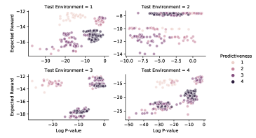
K.3 P-value and Generalization Analysis
In the semi-real experiment (see Section 6.4), we further analyze the generalization performance of each candidate set and its corresponding p-value returned by the invariance test. To distinguish the effects of invariance and predictiveness on the generalization performance (measured by the expected reward on a test environment), we partition the subsets into four groups depending on their performance on the training environments (1 is the least predictive and 4 is the most predictive).
Within each predictiveness group, the scatter plots in Figure 7 display a correlation between the p-value returned by the invariance test and the expected reward under a test environment. This result indicates that a policy that depends on a subset with a higher degree of invariance (higher p-value) tends to generalizes better to a new environment. The correlation is strongest in the test environment in which we could also observe the largest performance gap between invariant and non-invariant approaches, see Figure 5.
Appendix L
We now discuss an example (presented in Figure 8) that justifies Assumption 2. In this example, the variables and influence only the observed covariates but not the reward . This example would lead to the following problems in Proposition 1(ii) and Theorem 1.
First, the subsets and are both -invariant, but no set of size or more is -invariant. By symmetry, there is no guarantee that a -invariant set that is optimal in the training environments will also be optimal in a new test environment because e.g. might be optimal on the training data while is optimal on the test data. This then refutes the statement in Proposition 1(ii). Assumption 2 fixes this problem as it ensures the existence of a largest -invariant set which is a superset of all other -invariant sets (see the proof of Lemma 4), and rules out this example.
Second, there is no strongly non--invariant variable (see Definition 5) in this example and hence Assumption 3 does not guarantee the existence of a confounding removing environment. This implies that a set of environments can be arbitrary, for instance, it could be a singleton . In that case, Theorem 1(ii) would no longer hold (but Theorem 1(i) remains valid). We therefore require Assumption 2 for proving the results of Proposition 1(ii) and the second statement of Theorem 1(ii).