Introduction

Invariant Object Computation

Object recognition is one of the most fundamental cognitive tasks performed by the brain. A successful object recognition requires a brain to discriminate between different classes of objects despite variabilities in the stimulus space. For example, a mammalian visual system can recognize objects despite a variation in the orientation, position, and background context, etc. Such impressive robustness to noise is not only specific to visual object recognition, but also similar tasks done by other brain modalities. Auditory systems are able to recognize auditory ’objects’ such as songs, and languages, despite variabilities in the sound intensity, relative pitches, or sound textures (such as voice of a person). In general, human perception has to operate with discrete entities such as objects, faces, words, smells, and tasks. Hence, it is of fundamental interest to understand to evaluate the emergence of neural representations of these entities along the sensory hierarchies. Artificial intelligent systems aim to solve similar perceptual tasks. The recent success of Deep Networks has been foremost their ability to perform object recognition tasks despite the immense variabilities in the signals input representations, in both training and testing examples ^{krizhevsky2012imagenet}. An artificial face recognition tasks have to be done despite variabilities of facial expressions, image scale and occlusion, etc. Autonomous driving systems have to recognize objects in the driving environment fast and accurately, despite the various conditions such as speed of approach, location, confounding objects. Likewise, voice recognition systems need to overcome enormous variability in many stimulus dimensions. Indeed, it is a common practice in Machine Learning to augment the training set by performing a variety of transformations representing the natural inherent variability in the relevant object domain (’data augmentation’). Therefore, understanding how brain achieves an invariant object recognition tasks is not only important scientific challenge, but may also provide insight on how to improve artificial intelligent systems.

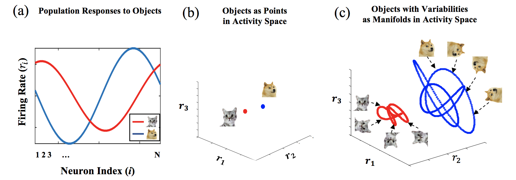
Figure 1: Activity Patterns as Points and Manifolds in the Neural State Space. (a) (Illustration) Firing Rate of N neurons (Neuron Index: 1,…,N), responding to two objects. Neural activity pattern shown as red line is a population response to a cat, and blue to a dog. (b) In the $N$ dimensional neural state space, the population response is a $N$-dimensional vector, representing a point. The blue line in (a) , representing a response to a dog, is a point, $\vec{r}_{dog}$, in $\mathbb{R}^{N}$space. Likewise, the red line in $(a)$ representing a cat is a point $\vec{r}_{cat}$ in $\mathbb{R}^{N}$space (only 3 axis are shown for illustration). (c) When the stimulus variabilities are introduced, such as change in orientation, the neural responses undergo a smooth change, causing the point representing each object in the state space move around, forming an object manifold in the neural state space. Blue manifold is a set of neural activities representing a dog at different orientations, and a red manifold is a set of neural activities representing a cat in different orientations.

Object Manifolds

Consider a set of neurons responding to different objects (Figure 3(a)). Without additional variabilities, two stimuli belonging to different classes are mapped into two points in the neural state space, $R^{N}$ (Figure. 3(b)). We will occasionally call each such point, a neural state or an activity pattern. If however, one varies continuously the physical parameters in the stimulus space which do not change the object class, e.g., orientation, location, distortion, the neural state vector will vary so that the set of neural states or activity patterns that correspond to an object can be thought of as a manifold in the neural state space (Figure 3(a)). In this geometrical perspective, object recognition and discrimination can be viewed as the the task of discriminating or recognition of manifolds. These manifolds vary as the signals propagate from one processing stage to another. We will therefore refer to these manifolds also as neural manifolds or manifold representations, when dealing with object manifolds as they are reflected in the state space of a specific neural stage.

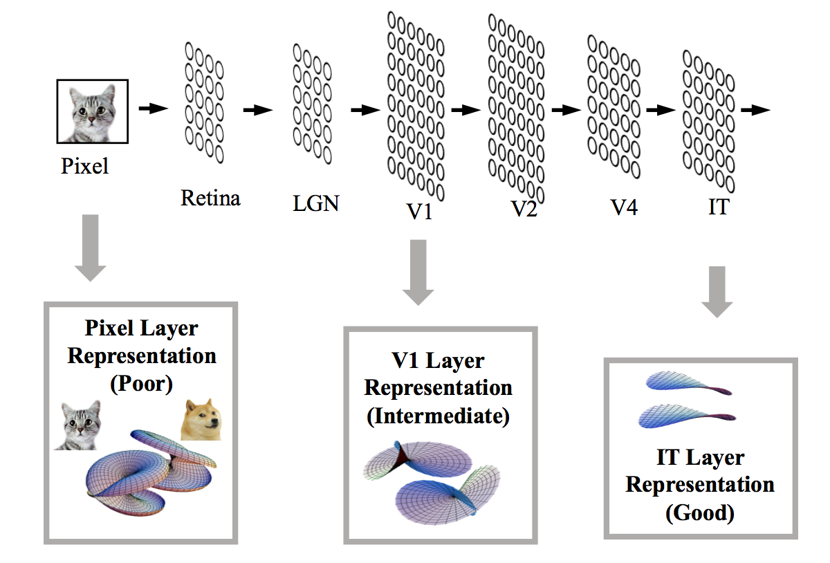
Figure 2: Untanglement of Object Manifolds in Sensory Hierarchy. Manifolds corresponding to different objects are thought to be highly tangled in the first stage of sensory processing (such as pixel layer representation), and undergo transformations across different layers in the sensory hierarchy and become more linearly separable in the downstream of the sensory processing.

Linear Separability of Manifolds

So, how does the brain and the deep networks overcome stimulus variabilities in object recognition? In the feedforward visual hierarchy, it has been suggested that the stages of nonlinear transformations reformat the object manifolds so that they become increasingly easier to be readout out by a simple downstream neural systems ^{dicarlo2007untangling}. The downstream circuit is assumed to implement a biologically plausible linear readout. Hence, the reformatting of object manifolds is translated as ’untangling’ them so that they are eventually amenable to be separated by a linear classifier. The idea that ’intermediate’ neural representations help to discriminate complex stimuli by a linear readout, has been applied to explain features of a variety of sensory representations in the brain (including ’mixed representations’ in prefrontal cortex^{rigotti2013importance}, sparse expansions in neocortical^{babadi2014sparseness}, memory allocations in hippocampal and cerebellar systems^{valiant2012hippocampus}). Deep Networks for object recognition has similarly employed an architecture where at the top layer a linear classifier operates as a readout of the networks.

Linear separation of neural manifolds can be described by a decision hyperplane that separates entire manifolds to one of the two sides of the hyperplane, fig. 3. The separating hyperplane is determined by the vector $\mathbf{w}$, a direction vector normal to the hyperplane. The components of this vectors are the synaptic weights of the Linear Readout, also known as the Perceptron, as it computes the weighted sum of each vector and thresholds the result to produce a binary output. One of the focus of this work is to evaluate what aspects of the the neural manifolds representation gives a better linear separability. Before continuing it is important to emphasize that by separating manifolds we mean separating all points on the manifolds according to a rule that assigns to all points belonging to a single manifold the same label. Thus, at any given time, the system classifies a single input vector.

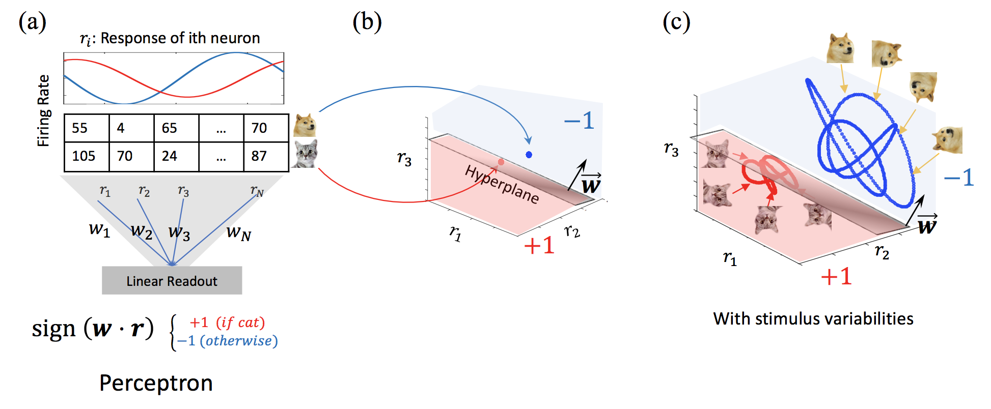
Figure 3: Invariant Object Discrimination as Linear Separation of Manifolds. (a) A perceptron with a weight $\mathbf{w}$, which can classify different objects corresponds to a hyperplane characterized by the orthogonal vector $\mathbf{w}$ which separates the two object points in the state space (b). (c) In this perspective, a perceptron weight $\mathbf{w}$, which can classify different objects with their variabilities, corresponds to a hyperplane characterized by the orthogonal vector $\mathbf{w}$, which separates the two object manifolds in the state space.

Theory of Linear Classification

Quantifying linear separability has been extensively studied in the context of linearly classifying isolated points. Perceptron capacity, first introduced by Cover ^{cover1965geometrical}. He asked the following question in his formulation of Cover’s Theorem. Suppose there are $P$ points in an N-dimensional ambient space, and they are in general position. Each of the point represent a distinct pattern, and half of the points are labeled positive, and the other half negative. Then, what is the maximum number of $P$ where most of the dichotomies are linearly separable? If there are only a few points, it is easy to find a linearly separable solution, and with an increasing number of points, it becomes harder to find linearly separable solution. When there are too many points, they become linearly non-separable. He derived an analytic formula for the probability that a random classification of P points in N dimensions can be implemented by perceptron as

$$\frac{C(P,N)}{2^{P}}=\frac{2\sum_{k=0}^{N-1}\left(\begin{array}[]{c}P-1\\ k\end{array}\right)}{2^{P}}$$ (1)

and the notion of perceptron capacity deals with the question of what is the maximum number of patterns allowed for linear such that almost all dichotomies are linearly separable (Figure 4). Cover’s perceptron capacity refers to the maximum number of patterns $P_{max}$ allowed per ambient dimension $N$, also known as load ($\alpha=P_{max}/N$),such that the probability of linear separability is larger than 0.5. VC dimension refers to the maximum load $\alpha$ such that the probability of linear separability is 1(Figure 4).

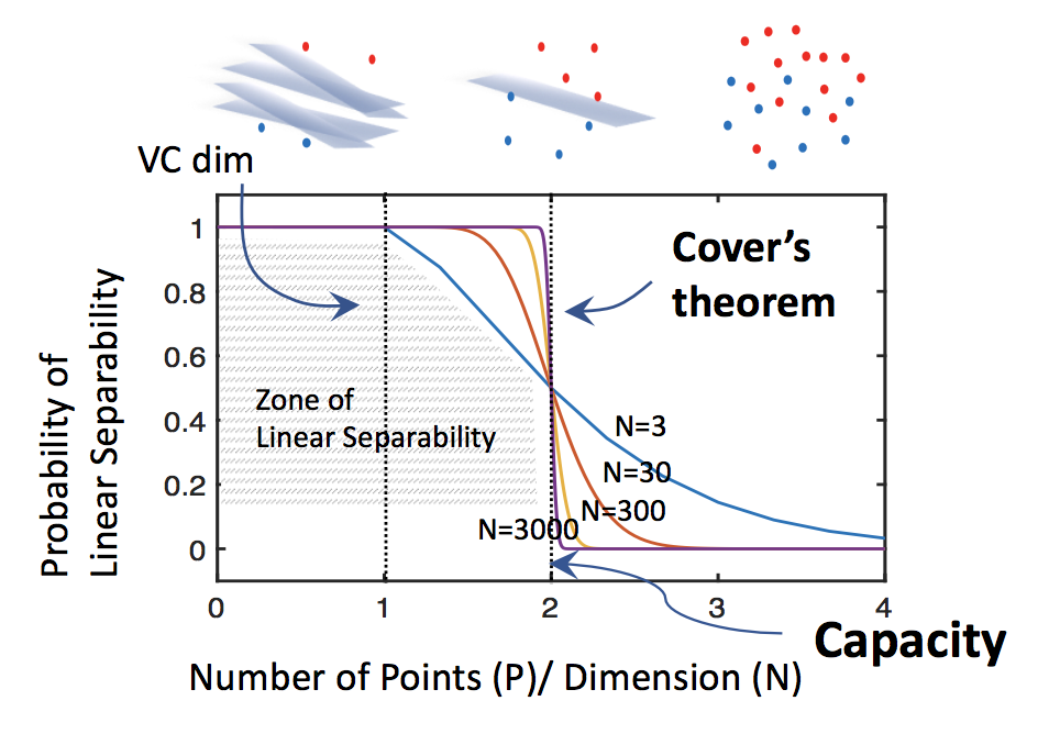
Figure 4: Linear Separability of Points: Cover’s Theorem of Perceptron Capacity. Cover’s theorem specifies the perceptron capacity for isolated points in general position, as the maximum number of points $P$ (in dimension $N$) for which at least half of the possible dichotomies have a linear classifier.

A statistical mechanical theory of the perceptron was first introduced by Elizabeth Gardner^{gardner1988space, gardner87}. Gardner’s theory is extremely important as it provides accurate estimates of the Perceptron capacity beyond the Cover theorem. In particular, the theory allows to evaluate the capacity for solutions with a given robustness measures. Similar to Support Vector Machines ^{vapnik1998statistical}. robustness of linear classifiers can be quantified by the margin, ie., the distance between the separating hyperplane and the closest point. And the solutions with maximum margins are known as the SVM solutions.

Formally, Gardner’s theory evaluates the maximal number of points in $R^{N}$ for which there is a vector $w$ that obeys the following set of inequalities

$$y^{\mu}\left(\vec{w}\cdot\vec{x}^{\mu}+b\right)/||\vec{w}||>\kappa\geq 0;\>y^{\mu}=\pm 1$$ (2)

Unlike Cover result, the answer to this question depends on the statistics of the inputs and labels. The simplest case is where all components $x_{i}^{\mu}$are iid with zero mean and finite variance (which can be taken as 1). (The shape of the distribution are less important as long as mild conditions are obeyed). The labels are randomly assigned to these points each with probability $1/2$ . Finally, the theory becomes exact in the the thermodynamic limit $N,P\rightarrow\infty$, while $\alpha,\kappa,=O(1)$ . Using replica theory in the theory of spin glasses (more detailed treatment is in the appendix to the chapter), Gardner has evaluated analytically the volume of possible solutions for a given load $\alpha$ and margin $\kappa$ . The volume is exponentially large (in $N$) below the capacity, $\alpha_{G}(\kappa)$ and is zero above it. The maximal margin solution is right at the border between the two regimes. Using the vanishing volume condition, Gardner obtained an elegant expression for the perceptron capacity with finite margin $\kappa$

$$\alpha_{G}(\kappa)=\left(\int_{-\kappa}^{\infty}Dt\left(t+\kappa\right)^{2}\right)^{-1}$$ (3)

where $Dt=\frac{\text{exp}\left(-\frac{1}{2}t^{2}\right)}{\left(2\pi\right)^{1/2}}\text{d}t$ (Figure. 5(a)). Furthermore, the Gardner framework allows for the calculation of fraction of support vectors on the margin, which has an important bearing on its robustness and generalization performance (Ref) (Figure. 5(b)).

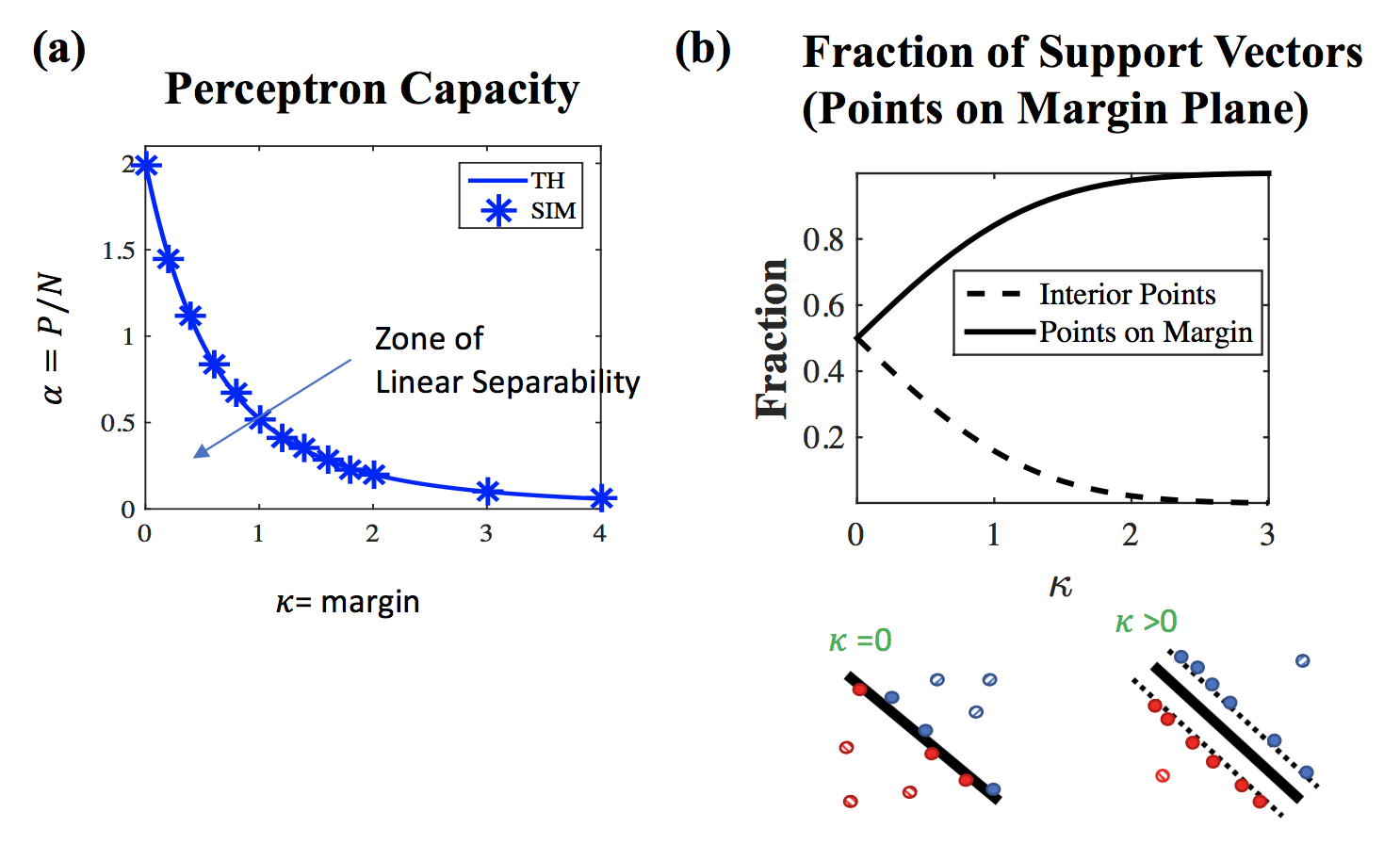
Figure 5: Gardner’s Perceptron Theory: Capacity and Support Vectors. (a) Gardner’s replica analysis specifies the perceptron capacity $\alpha=P/N$ as a function of margin $\kappa$. $P$ is number of points, $N$ is the network size. (b) The fraction of support vectors amongst the total number of points can be calculated as a function of margin $\kappa$ . At zero margin, half of the points are support vectors (black solid), and the other half are interior points, that are in the space shattered by the hyperplane (black dashed). The fraction of support vectors in crease with increasing margin $\kappa$.

Gardner theory is also applicable to more complex statistical ensembles, such as the case of sparse labels where the labels are not uniformly distributed. However, the current theory is inapplicable to the problem of manifold classification, where the strong correlations between points belonging to the same manifold is of primary importance. The thesis addresses the following questions:

1. What is the capacity of manifolds, and the nature of solution? What geometric features of the manifolds are relevant for the manifold capacity?

2. How to implement the practical aspects of analyzing data manifolds numerically? In order to test the manifold capacity with simulation, what is the most efficient algorithm to find a classification solution for manifolds? To get an estimate of the manifold capacity, how to numerically solve it?

3. What are the necessary extensions required to understand and analyze more realistic problems? We extend it to manifold classification problem with sparse labeling, correlation, classification with nonlinearities such as multilayer and nonlinear kernels, and apply the theory to realistic data.

Outline of Thesis

This thesis introduces a theory that generalizes Gardner’s analysis of perceptron capacity for isolated points to the perceptron capacity for manifolds. The theory assumes (most of the time) that the manifolds span a low dimensional hyperspace (strictly speaking the embedding dimension is held finite as $N\rightarrow\infty).$ In the following chapters, we introduce a set of investigations that lays groundwork for a comprehensive theory of linear manifold classification. In chapter 2, we provides the basic tools for applying the replica theory to compute linear classification of manifolds. Here we focus on the simple manifolds: line segments, $L_{2}$ balls, and $L_{p}$ balls. In chapter 3, we address the numerical question of how to solve max margin problems on manifolds, which consists of uncountable set of training examples. We use methods from Quadratic Semi-Infinite Programming (QSIP) to develop a novel algorithm denoted M4 (Max Margin Manifolds Machines). In chapter 4, we generalize the theory of chapter 2 to address more complex manifold geometries, for both smooth and non-smooth manifolds. In chapter 5, we present a set of important extensions of the theory to cover more realistic conditions, such as correlated manifolds, and sparse coding tasks. We also discuss extensions to nonlinear manifold classifications. Finally, we demonstrate how the theory can be applied to analyze deep networks for in visual object recognition.

Chapter 2: Linear Separation of $L_{p}$Balls

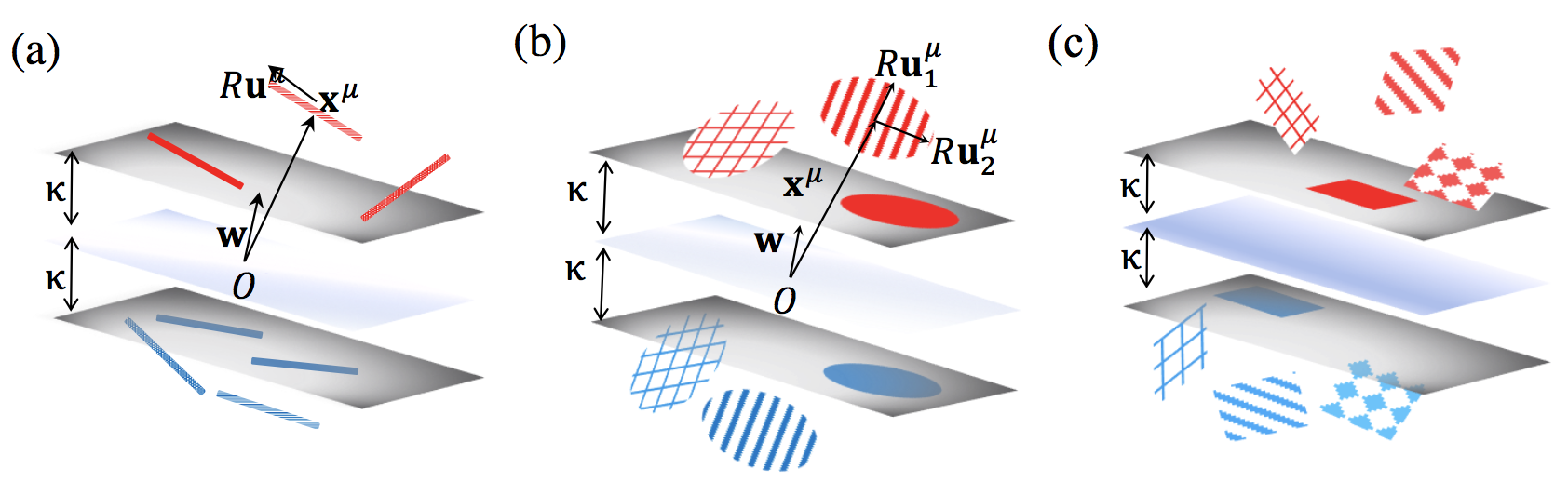
Figure 6: Linear Classification of $L_{p}$ balls. (a) Classification of line segments with length $2R$. (Example of $D=1$ balls with radius $R$). (b) Classification of $D$-dimensional $L_{2}$ balls with radius $R$. (c) Classification of $D$-dimensional $L_{1}$ balls with radius $R$.

In this chapter we lay the ground for the statistical mechanical theory of linear classification of manifolds. We consider manifolds which can be described as $L_{p}$ balls in $D$ dimensions with a radius $R$ . We write points on the manifolds as,

$$x^{\mu}=\left\{x_{0}^{\mu}+R\sum_{i=1}^{D}s_{i}u_{i}^{\mu}\right\}$$ (4)

where $x_{0}^{\mu}$ is the center of the $\mu$th ball, $\mu=1,...,P$. The axes of the balls are given by the D vectors $u_{i}^{\mu}$where $i=1,...,D$. The vector $\vec{s}$ parameterizes the point on the ball and obeys the constraint $||s||_{p}\leq 1$ . The case of $p=2$ corresponds to the usual Euclidean balls in $D$ dimensions. The case of $D=1$ is the special case of line segments with length $2R$. Other examples are shown in fig. 6. As we show in this chapter, linear classification of these balls corresponds to the requirements that the closest points on each manifolds obeys inequalities, eq 4 above. For the $L_{p}$ balls, with $1<p\leq\infty$1, this amounts to the following constraints (where we consider zero bias for simplicity)

$$h_{0}^{\mu}-R||\vec{h}^{\mu}||_{q}\geq\kappa,$$ (5)

$$q=p/(p-1),\;1<p<\infty$$ (6)

$$q=\infty\;0<p\leq 1$$ (7)

where $h_{0}^{\mu}=||\mathbf{w}||^{-1}y^{\mu}\mathbf{w}\cdot\mathbf{x}^{\mu}$ are the fields induced by the centers and $h_{i}^{\mu}=||\mathbf{w}||^{-1}y^{\mu}\mathbf{w}\cdot\mathbf{u_{i}}^{\mu}$ are the fields induced by the $i$ th basis vectors of $\mu$th manifold, $\kappa$ is the margin of the linear classifier.

Importantly, linear classification of manifolds depends on the geometric properties of the convex hulls of the data manifolds. Thus, when $p\leq 1$, the convex hull of the manifold becomes faceted, consisting of vertices, flat edges and faces. For these geometries, the constraints on the fields associated with a solution vector $\mathbf{w}$ becomes: $h_{0}^{\mu}-R\max_{i}\left\|h_{i}^{\mu}\right\|\geq\kappa$ for all $p<1$ (Fig. 6(c)).

The statistical mechanical theory evaluates the average of the log of solution volume,

$$V=\int_{\left\|\mathbf{w}\right\|^{2}=N}d^{N}\mathbf{w}\>\prod_{\mu=1}^{P}\Theta\left(h_{0}^{\mu}-R||\vec{h}^{\mu}||_{q}-\kappa\right).$$ (8)

and identifying the point of vanishing volume allowed us to evaluate the capacity, in the form of $\alpha_{B_{p}}(\kappa,R,D)$ for various norms $L_{p}$ . Beyond the capacity, the theory provides an important insight into the nature of the max margin solution. In particular it generalizes the notion of support vectors to support manifolds. As we show, some of the support manifolds are fully embedded in the margin hyperplanes, some are touching the planes in a single point, while in the case of $L_{1}$balls, they may have edges or faces in the hyperplanes. These properties have important implications for noise robustness of the solutions. Finally, these examples already reveal the tradeoff between $D$ and $R$, and the effect of large $R$ and large $D$. Specifically, we show that for large $D$ $L_{2}$ balls,

$$\alpha_{B}(\kappa,R,D\gg 1)=(1+R^{2})\alpha_{G}(\kappa+R\sqrt{D}),\,\ D\gg 1$$ (9)

relating linear separation of balls to linear separation of points with an additional effective margin $R\sqrt{D}$.

Chapter 3: The Max Margin Manifold Machine

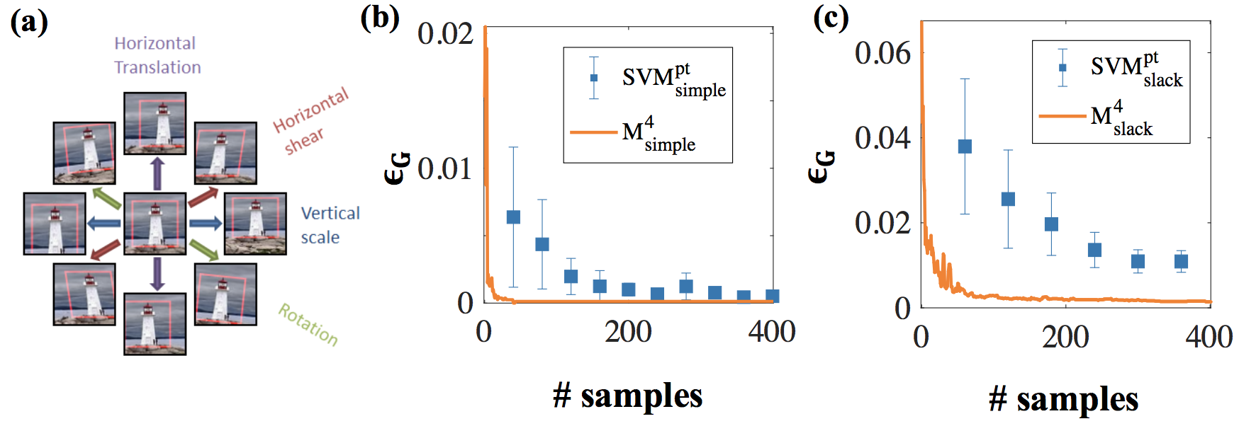
Figure 7: The Maximum Margin Manifold Machine Performance. (a) Object-based manifolds are created by affine transformations of images from ImageNet dataset. (b) Generalization error versus number of training samples, for the linear $SVM$ (blue markers) and the $M_{simple}^{4}$ algorithm, when the manifolds are in the separable regime. (b) Generalization error versus the number of training samples for slack-SVM (blue) and $M_{slack}^{4}$ algorithm when manifolds are in the non-separable regime (above capacity). Our $M_{simple}^{4}$ and $M_{slack}^{4}$ show superior generalization error performance for the same number of training samples.

Most learning algorithms assume the number of training examples is finite. In this work, we consider the problem of classifying data manifolds utilizing the underlying manifold structure consisting of an uncountable number of points. We propose an efficient iterative algorithm called $M^{4}$ that solves a quadratic semi-infinite programming problem to find the maximum margin solution. Our method is based upon a cutting-plane approach which converges to an approximate solution in a finite number of iterations. We provide a proof of convergence as well as a polynomial bound on the number of iterations and training examples required for a desired tolerance in the objective function. The efficiency and performance of $M^{4}$ are demonstrated on high-dimensional synthetic data in addition to object manifolds generated by continuous transformations of images from the ImageNet dataset. Our results indicate that $M^{4}$ is able to rapidly learn good classifiers and shows superior generalization performance than traditional support vector machines using data augmentation methods (Fig. 7).

Chapter 4: Linear Classification of General Low Dimensional Manifolds

In this chapter we generalize the perceptron capacity for the classification of manifolds further, to classification of general manifolds. The theory is exact in the thermodynamic limit, i.e., $N,P\rightarrow\infty$, $\alpha=P/N$ is finite as in the Gardner’s analysis. In addition, for the mean field theory to be exact, the dimensionality of the manifolds $D$ has to be finite in this limit (note: this holds except for the special case of parallel manifolds, section Parallel Spheres, where $D$ is proportional to $N$). To set the stage, we first consider linear classification capacity of $L_{2}$ ellipsoids. We present explicit analytical solution to the classification problem, and show that the capacity and solution properties depend in general on all $D$ radii. Like the balls, the max margin solution is characterized by two types of support ellipsoids (touching or fully embedded).

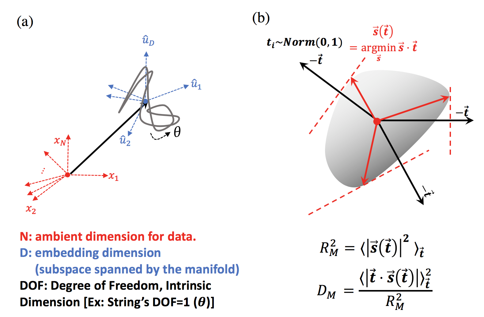
Figure 8: Manifold’s Sizes and Dimensions. (a) Dimensions of a Random String. A random string’s degree of freedom (intrinsic dimension) is 1, but is spanning $D$-dimensional (embedding dimension) and defined in $N$ ambient dimension. (b) Effective manifold radius $R_{M}$ and effective manifold dimension $D_{M}$, which are relevant properties for the manifold’s linear classification capacity.

Effective Sizes and Dimensions: In general, manifolds considered here are characterized by several dimensionalities. All points on all manifolds are in $\mathbb{R}^{N}$, so $N$ is the ambient dimension. All points on a given manifold (relative to its center) span $D$ dimensions, thus $D$ is the manifold embedding dimension. In addition, manifolds may be characterized by intrinsic dimensionality which may be much smaller than $D$. See Fig. 8(a) for an example of a string in $D$ dimension. This intrinsic dimension is important practically, but will not play an important role in the theory of linear classification. In addition to the above, the manifold classification properties may be described in certain regime by effective dimensions and effective size (Fig. 8(b)).

Here we present the results for ellipsoids in the important limit of large $D$. In this limit we find that the capacity can be well approximated as,

$$\alpha_{E}(\kappa,R)=(1+R_{E}^{2})\alpha_{G}(\kappa+R_{E}\sqrt{D_{E}}),\,\ D\gg 1$$ (10)

where $E$ stands for ellipsoids, and with effective ellipsoid radius $R_{E}$ and effective ellipsoid dimension $D_{E}$ given by,

$$R_{E}^{2}=\sum_{i=1}^{D}\frac{R_{i}^{4}}{(1+R_{i}^{2})^{2}}/\sum_{j=1}^{D}\frac{R_{j}^{2}}{(1+R_{j}^{2})^{2}}$$ (11)

$$D_{E}=\left(\sum_{i=1}^{D}\frac{R_{i}^{2}}{1+R_{i}^{2}}\right)^{2}/\sum_{i=1}^{D}\frac{R_{i}^{4}}{(1+R_{i}^{2})^{2}}$$ (12)

where $R_{i}$ are the different radii of the ellipsoid. Finally, when the radii are small, $R_{i}\ll 1$ (i.e., relative to the center norms which is normalized here to $1$). these quantities reduce to the simple formulae

$$R_{E}^{2}=\frac{\sum_{i}R_{i}^{4}}{\sum_{i}R_{i}^{2}}$$ (13)

$$D_{E}=\frac{(\sum_{i}R_{i}^{2})^{2}}{\sum_{i}R_{i}^{4}}=D_{svd}$$ (14)

where $D_{svd}$ is the participation ratio evaluated from the SVD of the ellipsoids (with a uniform measure). These results set the stage for a derivation of a theory applicable to general low dimensional manifolds. Briefly, general smooth convex manifolds behave qualitatively the same as the ellipsoids, for the geometric reason that they can either be interior to, fully embedded in or touching the margin planes.

Non-smooth manifold can have a large spectrum of overlaps with the planes (as the example of $L_{1}$ ball indicates). Nevertheless, we have derived self consistent mean field equations that describe the capacity (and solution properties) for a general manifold, and present numerical procedures to solve these equations iteratively. Here we briefly discuss the theoretical prediction for the limit of large $D$. In this regime, capacity is well approximated by

$$\alpha_{M}(\kappa)=(1+R_{M}^{2})\alpha_{G}(\kappa+R_{M}\sqrt{D_{M}}),\,\ D\gg 1$$ (15)

with self consistent equations for $R_{M}$ and $D_{M}$, which need to be solved numerically by iterative mean field methods. Remarkably, in the regime where $R_{M}\ll 1$, $R_{M}$ and $D_{M}$ simplify to the quantities shown in Fig. 8(b) and are related to the well known Gaussian Mean Width of convex bodies (Fig. 20).

An important application of this theory is finite point cloud manifolds that arise when subsampled points of each potentially continuous manifold is given. In this case, $R_{M}$ and $D_{M}$ (of the training manifolds) can be estimated from the given finite training set. The interesting question of how these quantities are related to the effective radius and dimension underlying full manifold is touched upon in the following section. An interesting example is the case of $L_{1}$balls in $D$ dimensions with radius $R$. In the limit of large $D$ and small $R$, the effective radius is simply $R$ but the dimension is

$$D_{M}=2\log D$$ (16)

In general, in other point cloud manifolds we expect that $D_{M}\propto\log m$ where $m$ is the number of samples per manifold.

Infinite size manifolds: Finally, it should be noted that as the manifold size grows to infinity (in all dimensions), their geometric details don’t matter; only the number of dimensions they span. Here we obtain

$$D_{M}\rightarrow D$$ (17)

reflecting the need of the classifying weight vector to be orthogonal to all the $DP$ dimensional hyperspace that the manifolds span, namely the capacity reduces to

$$\alpha_{M}=\frac{1}{D}$$ (18)

where $D$ denotes the embedding dimensions of the manifolds (where we assume for simplicity that the manifolds are not bounded in any of the $D$ directions).

Chapter 5: Extensions

Figure 9: Extensions of Manifold Classification Theory. (a) Classification of Correlated Manifolds. (b) Classification of Mixtures of Manifolds. (c) Sparse Coding (Classification with Sparse Labels) and Object Recognition Limit (One versus All Classification). (d) Extension to Kernel Framework. (Red/black) $2D$ disks in the kernel input space, transformed to (blue/black) $5D$ manifolds in the quadratic kernel’s feature space.

In Chapter 5, we further extend the theory in directions likely relevant to applications to real data. We have extended our general manifold classification theory to incorporate correlated manifolds, mixtures of manifold geometries, sparse labels and nonlinear classification, see Fig. 9. We highlight here briefly several important results. 1. Correlated manifolds: when manifold axes are strongly parallel (fig. 9(a)) we expect the capacity to be relatively large. For example if their spanning spaces are fully aligned but they are large in extent, $\mathbf{w}$ can solve the problem by orthogonalize to the $D$ common directions (rather than $DP$ in the uncorrelated case). Interestingly, for high dimensional parallel balls we find a phase transition whereby above some finite critical radius the max margin solution fully orthogonalize to the manifolds subspace. In real data we expect positive correlations but not full alignment of the different manifolds.

2. Sparse labels: In this case, the fraction of say plus manifolds, $f$, is smaller than that of the minus ones. In many real life tasks this is to be expected. An extreme case is that of object recognition task defined as classifying one manifold as one and the rest as minus one. This can be viewed as a binary classification with $f=\frac{1}{P}$ . As in Gardner’s theory the capacity grows as $f\rightarrow 0$. However, we show that the size of the manifolds substantially limits this growth. For instance, in balls with large radius $R$ , the $f$ is small but larger than $1/R$ the capacity remains of order unity.

3. Nonlinear manifold separation: We consider two schemes of two layer classification of manifolds in cases where they are not linearly separable. One is in the form of a nonlinear kernel, similar to Kernel SVM. For this we present a version of the $M^{4}$algorithm in a ’dual’ form, appropriate for kernels. We briefly discuss the effect of the kernel on the geometry of the manifold and the classification capacity. The second architecture is that of hidden layer of binary units, forming a sparse intermediate representation of the manifolds. We show how this extra layer formed by unsupervised learning can enhance the capacity and robustness of the classification of the manifolds.

4. Generalization properties : Computation with manifolds raises a specific type of generalization problem, namely how training with a subsampled training points perform when new points from the same underlying manifolds are presented in the test phase. Exact analytical expression for the generalization error is complicated; also the error depends on the assumed sampling measure on the manifold (whereas the separability problem is measure invariant). However, in the case of linearly separable manifolds with high $D$ we can use the insight from the above theory (the notions of effective dimensions and radii) to derive a particularly simple approximation. Assume $\alpha$ is such that the full manifolds are linearly separable with a max margin $\kappa$. Then the generalization error will eventually vanish as more samples per manifold , $m$ , are presented. In the limit of large $m$ , we obtain,

$$\epsilon_{g}(m)\propto\frac{\exp[-\kappa\sqrt{2\log m}]}{m}$$ (19)

Interestingly, this decay is faster than the generic power law, $\epsilon_{g}(m)\propto m^{-1}$ of generalization bounds in linearly separable problem and reflects the presence of finite margin of the entire manifold. We also discuss the generalization error of subsampled manifolds in the case where the full manifolds are not linearly separable.

5. Application to Deep Networks: We close this section by applying some of the theoretical concepts to Deep Networks trained to perform visual object recognition tasks. We show how the theory can be used to characterize the change in the geometry of the manifolds, and changes in the manifold correlation structure at different stages of the network (using ImageNet^{deng2009imagenet} as an example).

Conclusion and Future Direction

In this thesis, we generalized Gardner’s theory of linear classification of points to the classification of general randomly oriented low dimensional manifolds. The theory, exact in the thermodynamic limit, describes the relation between the detailed geometry of the convex hulls of the data manifolds and the ability to linearly classify them. The problem simplifies considerably when the manifold dimension is high. In this limit, the classification properties depend on two geometric parameters of the convex hulls: the effective dimension $D_{M}$ and effective radius $R_{M}$. In high dimensional manifold with small sizes, capacity depends on $R_{M}$ and $D_{M}$ mainly through the scaling relation $R_{M}\sqrt{D_{M}}$. This quantity is related to the well known Gaussian Mean Width of convex bodies. Optimal solution exhibits support manifold structures with potential consequences for noise robustness. We developed a novel efficient training algorithm, the Maximum Margin Manifold Machines, for finding the maximum margin solution for classifying manifolds with uncountable number of training samples, and provide convergence proof with polynomial bounds on the number of iterations required for convergence. Our theory has been extended to incorporate correlations in the manifolds, mixtures of shapes, sparse coding, nonlinear processing such as multilayer network or kernel framework, as well as an analysis of manifold generalization error. With these extensions, our theory provides qualitative and quantitative measures for assessing the ability to decode object information from the different stages of Deep biological and artificial neural networks.

Ongoing work includes suggesting design principles for deep networks by taking into account the network size, dimension, sparsity, as well as role of nonlinearities in reformatting of the manifolds such that the capacity is increased. Whether manifold capacity can be used as an object function of the training of a network is an interesting question to pursue. We are exploring applications of our theory on several neural data bases from IT and other areas in visual cortex, responding to different object stimuli with a variety of physical transformations. We hope that our theory will provide new insights into the computational principles underlying processing of sensory representations in the brain. As manifold representations of the sensory world are ubiquitous in both biological and artificial neural systems, exciting future work lies ahead.

Linear Classification of Spherical Manifolds

High-level perception in the brain involves classifying or identifying objects which are represented by continuous manifolds of neuronal states in all stages of sensory hierarchies ^{dicarlo2007untangling, pagan2013signals, alemi2013multifeatural, bizley2013and, meyers2015intelligent, schwarzlose2008distribution, gottfried2010central} Each state in an object manifold corresponds to the vector of firing rates of responses to a particular variant of physical attributes which do not change object’s identity, e.g., intensity, location, scale, and orientation. It has been hypothesized that object identity can be decoded from high level representations, but not from low level ones, by simple downstream readout networks ^{hung2005fast, dicarlo2007untangling, pagan2013signals, freiwald2010functional, cadieu2014deep, kobatake1994neuronal, rust2010selectivity, schwarzlose2008distribution}. A particularly simple decoder is the perceptron, which performs classification by thresholding a linear weighted sum of its input activities ^{minsky1987perceptrons, gardnerEPL}. However, it is unclear what makes certain representations well suited for invariant decoding by simple readouts such as perceptrons. Similar questions apply to the hierarchy of artificial deep neural networks for object recognition ^{serre2005object, goodfellow2009measuring, ranzato2007unsupervised, bengio2009learning, cadieu2014deep}. Thus, a complete theory of perception requires characterizing the ability of linear readout networks to classify objects from variable neural responses in their upstream layer.

A theoretical understanding of the perceptron was pioneered by Elizabeth Gardner who formulated it as a statistical mechanics problem and analyzed it using replica theory ^{gardner1988space, engel2001statistical, advani2013statistical, brunel2004optimal, sompolinsky1990learning, opper1991generalization, rubin2010theory, amit1989perceptron, monasson1992properties}. In this work, we generalize the statistical mechanical analysis and establish a theory of linear classification of manifolds synthesizing statistical and geometric properties of high dimensional signals. We apply the theory to simple classes of manifolds and show how changes in the dimensionality, size, and shape of the object manifolds affect their readout by downstream perceptrons.

Line Segments

One-dimensional object manifolds arise naturally from variation of stimulus intensity, such as visual contrast, which leads to approximate linear modulation of the neuronal responses of each object. We model these manifolds as line segments and consider classifying $P$ such segments in $N$ dimensions, expressed as $\left\{\mathbf{x}_{0}^{\mu}+Rs\mathbf{u}^{\mu}\right\}$, $-1\leq s\leq 1$, $\mu=1,...,P$. The $N$-dimensional vectors $\mathbf{x}^{\mu}\in\mathbb{R}^{N}$ and $\mathbf{u}^{\mu}\in\mathbb{R}^{N}$ denote respectively, the centers and directions of the $\mu$-th segment, and the scalar $s$ parameterizes the continuum of points along the segment. The parameter $R$ measures the extent of the segments relative to the distance between the centers (Fig. 10).

We seek to partition the different line segments into two classes defined by binary labels $y^{\mu}=\pm 1$ . To classify the segments, a weight vector $\mathbf{w}\in\mathcal{R}^{N}$ must obey $y^{\mu}\mathbf{w}\cdot\left(\mathbf{x}^{\mu}+Rs\mathbf{u}^{\mu}\right)\geq\kappa$ for all $\mu$ and $s$. The parameter $\kappa\geq 0$ is known as the margin; in general, a larger $\kappa$ indicates that the perceptron solution will be more robust to noise and display better generalization properties ^{vapnik1998statistical}. Hence, we are interested in maximum margin solutions, i.e., weight vectors $\mathbf{w}$ that yield the maximum possible value for $\kappa$. Since line segments are convex, only the endpoints of each line segment need to be checked, namely $\min\,h_{0}^{\mu}\pm Rh^{\mu}=h_{0}^{\mu}-R\left|h^{\mu}\right|\geq\kappa$ where $h_{0}^{\mu}=||\mathbf{w}||^{-1}y^{\mu}\mathbf{w}\cdot\mathbf{x}^{\mu}$ are the fields induced by the centers and $h^{\mu}=||\mathbf{w}||^{-1}y^{\mu}\mathbf{w}\cdot\mathbf{u}^{\mu}$ are the fields induced by the line directions.

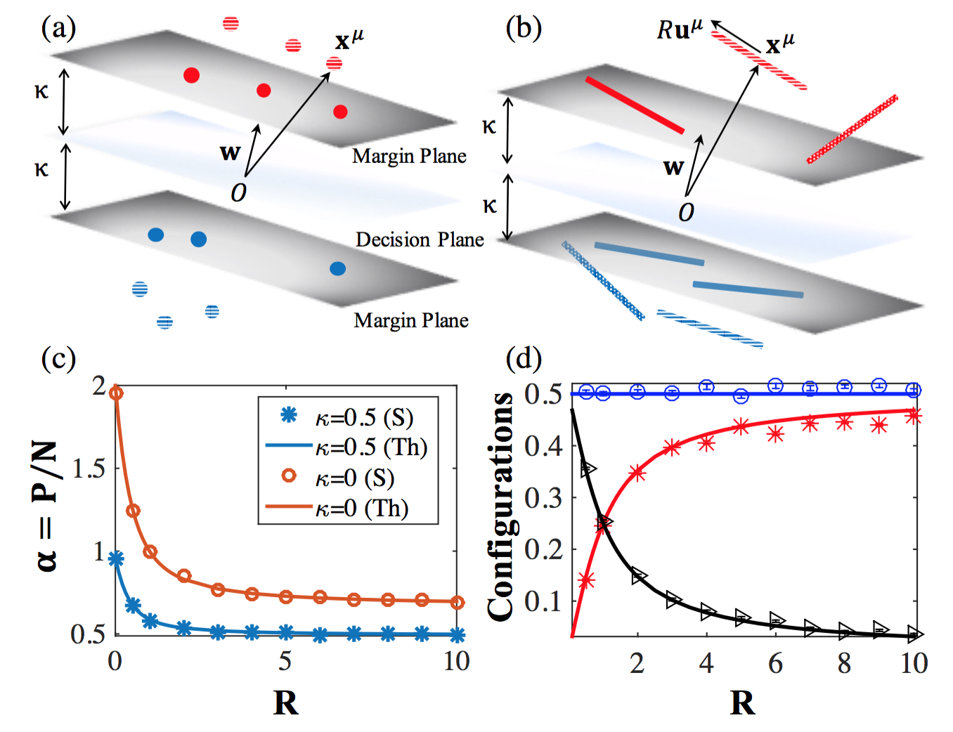
Figure 10: (a) Linear classification of points. (solid) points on the margin, (striped) internal points. (b) Linear classification of line segments. (solid) lines embedded in the margin, (dotted) lines touching the margin, (striped) interior lines. (c) Capacity $\alpha=P/N$ of a network $N=200$ as a function of $R$ with margins $\kappa=0$ (red) and $\kappa=0.5$ (blue). Theoretical predictions (lines) and numerical simulation (markers, see Appendix for details) are shown. (d) Fraction of different line configurations at capacity with $\kappa=0$. (red) lines in the margin, (blue) lines touching the margin, (black) internal lines.

Replica Theory

The existence of a weight vector $\mathbf{w}$ that can successfully classify the line segments depends upon the statistics of the segments. We consider random line segments where the components of $\mathbf{x}^{\mu}$ and $\mathbf{u}^{\mu}$ are i.i.d. Gaussians with zero mean and unit variance, and random binary labels $y^{\mu}$. We study the thermodynamic limit where the dimensionality $N\rightarrow\infty$ and number of segments $P\rightarrow\infty$ with finite $\alpha=P/N$ and $R$. Following Gardner ^{gardner1988space} we compute the average of $\log V$ where $V$ is the volume of the space of perceptron solutions:

$$V=\int_{\left\|\mathbf{w}\right\|^{2}=N}d^{N}\mathbf{w}\>\prod_{\mu=1}^{P}\Theta\left(h_{0}^{\mu}-R\left\|h^{\mu}\right\|-\kappa\right).$$ (20)

$\Theta(x)$ is the Heaviside step function. According to replica theory, the fields are described as sums of random Gaussian fields $h_{0}^{\mu}=t_{0}^{\mu}+z_{0}^{\mu}$ and $h^{\mu}=t^{\mu}+z^{\mu}$ where $t_{0}$ and $t$ are quenched components arising from fluctuations in the input vectors $\mathbf{x}^{\mu}$ and $\mathbf{u}^{\mu}$ respectively, and the $z_{0}$, $z$ fields represent the variability in $h_{0}^{\mu}$ and $h^{\mu}$ resulting from different solutions of $\mathbf{w}$. These fields must obey the constraint $z_{0}+t_{0}-R\left|z+t\right|\geq\kappa.$ The capacity function $\alpha_{L}(\kappa,R)$ (the subscript $L$ denotes the line) describes for which $P/N$ ratio the perceptron solution volume shrinks to a unique weight vector. The reciprocal of the capacity is given by the replica symmetric calculation (details provided in the Appendix Perceptron Capacity of Line Segments.):

$$\alpha_{L}^{-1}(\kappa,R)=\left\langle\min_{z_{0}+t_{0}-R\left|z+t\right|\geq\kappa}\frac{1}{2}\left[z_{0}^{2}+z^{2}\right]\right\rangle_{t_{0},t}$$ (21)

where the average is over the Gaussian statistics of $t_{0}$ and $t$. To compute Eq. (21), three regimes need to be considered. First, when $t_{0}$ is large enough so that $t_{0}>\kappa+R\left|t\right|$, the minimum occurs at $z_{0}=z=0$ which does not contribute to the capacity. In this regime, $h_{0}^{\mu}>\kappa$ and $h^{\mu}>0$ implying that neither of the two segment endpoints reach the margin. In the other extreme, when $t_{0}<\kappa-R^{-1}|t|$, the minimum is given by $z_{0}=\kappa-t_{0}$ and $z=-\left|t\right|$, i.e. $h_{0}^{\mu}=\kappa$ and $h^{\mu}=0$ indicating that both endpoints of the line segment lie on the margin planes. In the intermediate regime where $\kappa-R^{-1}\left|t\right|<t_{0}<\kappa+R\left|t\right|$, $z_{0}=\kappa-t_{0}+R|z+t$—, i.e., $h_{0}^{\mu}-R|h^{\mu}|=\kappa$ but $h_{0}^{\mu}>\kappa$, corresponding to only one of the line segment endpoints touching the margin. In this regime, the solution is given by minimizing the function $(R\left|z+t\right|+\kappa-t_{0})^{2}+z^{2}$ with respect to $z$. Combining these contributions, we can write the perceptron capacity of line segments:

$$\alpha_{L}^{-1}(\kappa,R) = \int_{-\infty}^{\infty}Dt\int_{\kappa-R^{-1}|t|}^{\kappa+R|t|}Dt_{0}\frac{\left(R\left|t\right|+\kappa-t_{0}\right)^{2}}{R^{2}+1}$$ (22)

$$+ \int_{-\infty}^{\infty}Dt\int_{-\infty}^{\kappa-R^{-1}|t|}Dt_{0}\left[(\kappa-t_{0})^{2}+t^{2}\right]\quad\quad$$

with integrations over the Gaussian measure, $Dx\equiv\frac{1}{\sqrt{2\pi}}e^{-\frac{1}{2}x^{2}}dx$. It is instructive to consider special limits. When $R\rightarrow 0,$ Eq. (22) reduces to $\alpha_{L}(\kappa,0)=\alpha_{0}(\kappa)$ where $\alpha_{0}(\kappa)$ is Gardner’s original capacity result for perceptrons classifying $P$ points (the subscript $0$ stands for zero-dimensional manifolds) with margin $\kappa$ 10-(a). Interestingly, when $R=1$, then $\alpha_{L}(\kappa,1)=\frac{1}{2}\alpha_{0}(\kappa/\sqrt{2})$. This is because when $R=1$ there are no statistical correlations between the line segment endpoints and the problem becomes equivalent to classifying $2P$ random points with average norm $\sqrt{2N}$ .

Finally, when $R\rightarrow\infty$, the capacity is further reduced: $\alpha_{L}^{-1}(\kappa,\infty)=\alpha_{0}^{-1}(\kappa)+1$. This is because when $R$ is large, the segments become unbounded lines. In this case, the only solution is for $\mathbf{w}$ to be orthogonal to all $P$ line directions. The problem is then equivalent to classifying $P$ center points in the $N-P$ null space of the line directions, so that at capacity $P=\alpha_{0}(\kappa)(N-P)$.

We see this most simply at zero margin, $\kappa=0$. In this case, Eq. (22) reduces to a simple analytic expression for the capacity: $\alpha_{L}^{-1}(0,R)=\frac{1}{2}+\frac{2}{\pi}\arctan R$ (Appendix Perceptron Capacity of Line Segments.). The capacity is seen to decrease from $\alpha_{L}(0,R=0)=2$ to $\alpha_{L}(0,R=1)=1$ and $\alpha_{L}(0,R=\infty)=\frac{2}{3}$ for unbounded lines. We have also calculated analytically the distribution of the center and direction fields $h_{0}^{\mu}$ and $h^{\mu}$ ^{abbott1989universality}. The distribution consists of three contributions, corresponding to the regimes that determine the capacity. One component corresponds to line segments fully embedded in these planes. The fraction of these manifolds is simply the volume of phase space of $t$ and $t_{0}$ in the last term of Eq. (22). Another fraction, given by the volume of phase space in the first integral of (22) corresponds to line segments touching the margin planes at only one endpoint. The remainder of the manifolds are those interior to the margin planes. Fig. 10 shows that our theoretical calculations correspond nicely with our numerical simulations for the perceptron capacity of line segments, even with modest input dimensionality $N=200$. Note that as $R\rightarrow\infty$, half of the manifolds lie in the plane while half only touch it; however, the angles between these segments and the margin planes approach zero in this limit. As $R\rightarrow 0$ , half of the points lie in the plane ^{abbott1989universality}.

$D$-dimensional Balls

Higher dimensional manifolds arise from multiple sources of variability and their nonlinear effects on the neural responses. An example is varying stimulus orientation, resulting in two-dimensional object manifolds under the cosine tuning function (Fig. 11(a)). Linear classification of these manifolds depends only upon the properties of their convex hulls ^{de2000computational}. We consider simple convex hull geometries as $D$-dimensional balls embedded in $N$-dimensions: $\left\{\mathbf{x_{0}}^{\mu}+R\sum_{i=1}^{D}s_{i}\mathbf{u}_{i}^{\mu}\right\}$, so that the $\mu$-th manifold is centered at the vector $\mathbf{x}^{\mu}\in\mathbb{R}^{N}$ and its extent is described by a set of $D$ basis vectors $\left\{\mathbf{u}_{i}^{\mu}\in\mathbb{R}^{N},\>i=1,...,D\right\}$. The points in each manifold are parameterized by the $D$-dimensional vector $\vec{s}\in\mathbb{R}^{D}$ whose Euclidean norm is constrained by: $\left\|\vec{s}\right\|\leq 1$ and the radius of the balls are quantified by $R$ .

Statistically, all components of $\mathbf{x}_{0}^{\mu}$ and $\mathbf{u}_{i}^{\mu}$ are i.i.d. Gaussian random variables with zero mean and unit variance. We define $h_{0}^{\mu}=N^{-1/2}y^{\mu}\mathbf{w}\cdot\mathbf{x}^{\mu}$ as the field induced by the manifold centers and $h_{i}^{\mu}=N^{-1/2}y^{\mu}\mathbf{w}\cdot\mathbf{u}_{i}^{\mu}$ as the $D$ fields induced by each of the basis vectors and with normalization $\left\|\mathbf{w}\right\|=\sqrt{N}$. To classify all the points on the manifolds correctly with margin $\kappa$, $\mathbf{w}\in\mathbb{R}^{N}$ must satisfy the inequality $h_{0}^{\mu}-R||\vec{h}^{\mu}||\geq\kappa$ where $||\vec{h}^{\mu}||$ is the Euclidean norm of the $D$-dimensional vector $\vec{h}^{\mu}$ whose components are $h_{i}^{\mu}$ . This corresponds to the requirement that the field induced by the points on the $\mu$-th manifold with the smallest projection on $\mathbf{w}$ be larger than the margin $\kappa$.

We solve the replica theory in the limit of $N,\,P\rightarrow\infty$ with finite $\alpha=P/N$, $D$, and $R$. The fields for each of the manifolds can be written as sums of Gaussian quenched and entropic components, $\left(t_{0}\in\mathbb{R},\>\vec{t}\in\mathbb{R}^{D}\right)$ and $\left(z_{0}\in\mathbb{R},\>\vec{z}\in\mathbb{R}^{D}\right)$ , respectively. The capacity for $D$-dimensional manifolds is given by the replica symmetric calculation (Appendix Perceptron Capacity of $D$-dimensional Balls):

$$\alpha_{B}^{-1}(\kappa,R,D)=\left\langle\min_{t_{0}+z_{0}-R\left\|\vec{t}+\vec{z}\right\|>\kappa}\frac{1}{2}\left[z_{0}^{2}+\left\|\vec{z}\right\|^{2}\right]\right\rangle_{t_{0},\vec{t}}$$ (23)

where $B$ stands for $L_{2}$balls. The capacity calculation can be partitioned into three regimes. For large $t_{0}>\kappa+Rt$, where $t=\left\|\vec{t}\right\|$, $z_{0}=0$ and $\vec{z}=0$ corresponding to manifolds which lie interior to the margin planes of the perceptron. On the other hand, when $t_{0}<\kappa-R^{-1}t$, the minimum is obtained at $z_{0}=\kappa-t_{0}$ and $\vec{z}=-\vec{t}$ corresponding to manifolds which are fully embedded in the margin planes. Finally, in the intermediate regime, when $\kappa-R^{-1}t<t_{0}<\kappa+Rt$, $z_{0}=R\left\|\vec{t}+\vec{z}\right\|-t_{0}+\kappa$ but $\vec{z}\neq-\vec{t}$ indicating that these manifolds only touch the margin plane. Decomposing the capacity over these regimes and integrating out the angular components, the capacity of the perceptron can be written as:

$$\alpha_{B}^{-1}(\kappa,R,D) = \int_{0}^{\infty}dt\,\chi_{D}(t)\int_{\kappa-\frac{1}{R}t}^{\kappa+Rt}Dt_{0}\frac{\left(Rt+\kappa-t_{0}\right)^{2}}{R^{2}+1}$$ (24)

$$+ \int_{0}^{\infty}dt\,\chi_{D}(t)\int_{-\infty}^{\kappa-\frac{1}{R}t}Dt_{0}\left[\left(\kappa-t_{0}\right)^{2}+t^{2}\right]\qquad$$

where $\chi_{D}(t)=\frac{2^{1-\frac{D}{2}}}{\Gamma(\frac{D}{2})}t^{D-1}e^{-\frac{1}{2}t^{2}}$ is the D-Dimensional Chi probability density function. For large $R\rightarrow\infty$, Eq. (24) reduces to: $\alpha_{B}^{-1}(\kappa,R=\infty,D)=\alpha_{0}^{-1}(\kappa)+D$ which indicates that $\mathbf{w}$ must be in the null space of the $PD$ basis vectors $\left\{\mathbf{u}_{i}^{\mu}\right\}$ in this limit. This case is equivalent to the classification of $P$ points (the projections of the manifold centers) by a perceptron in the $N-PD$ dimensional null space.

To probe the fields, we consider the joint distribution of the field induced by the center, $h_{0}$, and the norm of the fields induced by the manifold directions, $h\equiv\left\|\vec{h}\right\|$ . There are three contributions. The first term corresponds to $h_{0}-Rh>\kappa$, i.e. balls that lie interior to the perceptron margin planes; the second component corresponds to $h_{0}-Rh=\kappa$ but $h>0$, i.e. balls that touch the margin planes; and the third contribution represents the fraction of balls obeying $h_{0}=\kappa$ and $h=0$, i.e. balls fully embedded in the margin. The dependence of these contributions on $R$ for $D=2$ is shown in Fig. 11(b). Interestingly, when $\kappa=0$ , the case of $R=1$ is particularly simple for all $D$ . The capacity is $\alpha_{B}(R=1,D)=2/(D+1)$ ; in addition, the fraction of embedded and interior balls are equal and the fraction of touching balls have a maximum, see Fig. 11(b) and Appendix.

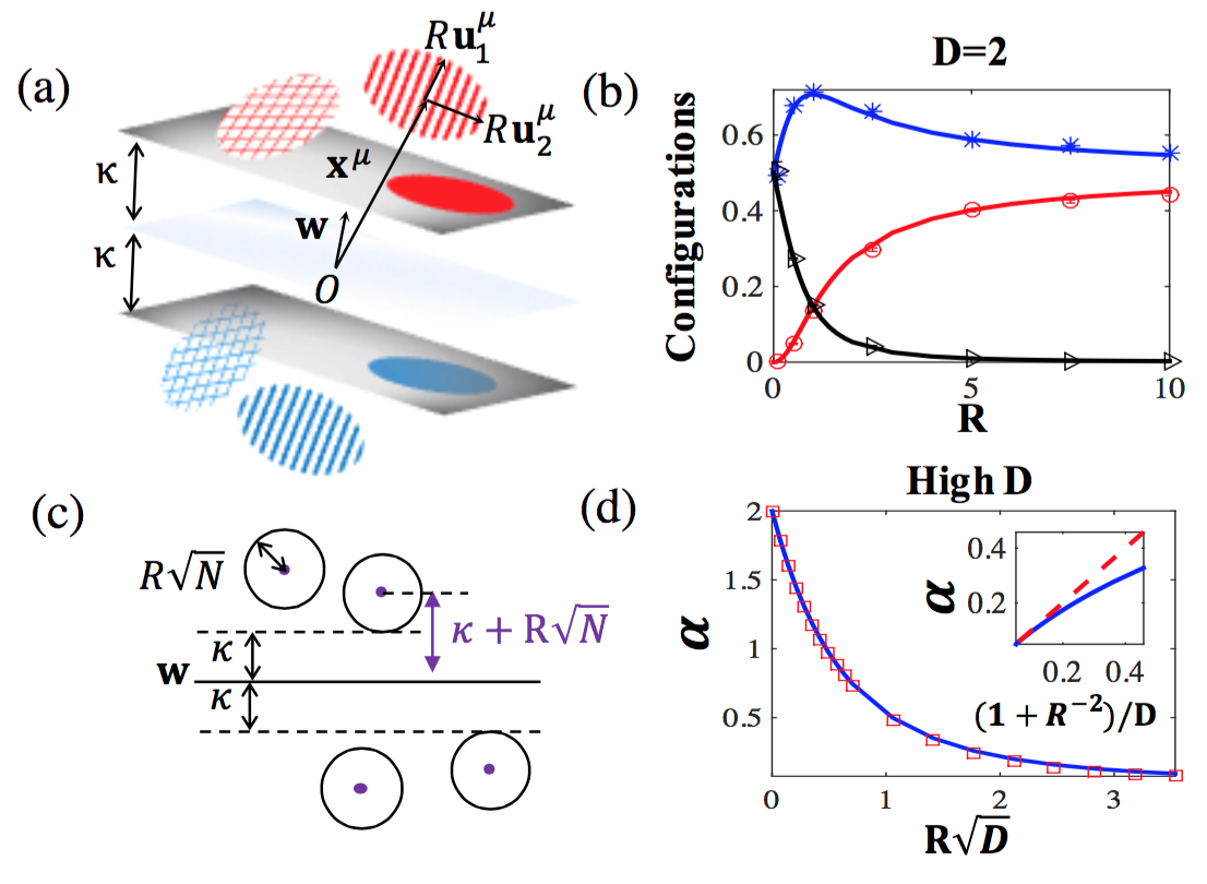
Figure 11: Random $D$-dimensional balls: (a) Linear classification of $D=2$ balls. (b) Fraction of 2-$D$ ball configurations as a function of $R$ at capacity with $\kappa=0$, comparing theory (lines) with simulations (markers). (red) balls embedded in the plane, (blue) balls touching the plane, (black) interior balls. (c) Linear classification of balls with $D=N$ at margin $\kappa$ (black circles) is equivalent to point classification of centers with effective margin $\kappa+R\sqrt{N}$ (purple points). (d) Capacity $\alpha=P/N$ for $\kappa=0$ for large $D=50$ and $R\propto D^{-1/2}$ as a function of $R\sqrt{D}$. (blue solid) $\alpha_{B}(\kappa=0,R,D)$ compared with $\alpha_{0}(\kappa=R\sqrt{D})$ (red square). (Inset) Capacity $\alpha$ at $\kappa=0$ for $0.35\leq R\leq 20$ and $D=20$: (blue) theoretical $\alpha$ compared with approximate form $(1+R^{-2})/D$ (red dashed).

In a number of realistic problems, the dimensionality $D$ of the object manifolds could be quite large. Hence, we analyze the limit $D\gg 1$. In this situation, for the capacity to remain finite, $R$ has to be small, scaling as $R\propto D^{-\frac{1}{2}}$, and the capacity is $\alpha_{B}(\kappa,R,D)\approx\alpha_{0}(\kappa+R\sqrt{D})$. In other words, the problem of separating $P$ high dimensional balls with margin $\kappa$ is equivalent to separating $P$ points but with a margin $\kappa+R\sqrt{D}$. This is because when the distance of the closest point on the $D$-dimensional ball to the margin plane is $\kappa$, the distance of the center is $\kappa+R\sqrt{D}$ (see Fig. 11). When $R$ is larger, the capacity vanishes as $\alpha_{B}(0,R,D)\approx\left(1+R^{-2}\right)/D$. When $D$ is large, making $\mathbf{w}$ orthogonal to a significant fraction of high dimensional manifolds incurs a prohibitive loss in the effective dimensionality. Hence, in this limit, the fraction of manifolds that lie in the margin plane is zero. Interestingly, when $R$ is sufficiently large, $R\propto\sqrt{D}$, it becomes advantageous for $\mathbf{w}$ to be orthogonal to a finite fraction of the manifolds.

$L_{p}$ Balls

To study the effect of changing the geometrical shape of the manifolds, we replace the Euclidean norm constraint on the manifold boundary by a constraint on their $L_{p}$ norm. Specifically, we consider $D$-dimensional manifolds $\left\{\mathbf{x}_{0}^{\mu}+R\sum_{i=1}^{D}s_{i}\mathbf{u}_{i}^{\mu}\right\}$ where the $D$ dimensional vector $\vec{s}$ parameterizing points on the manifolds is constrained: $\left\|\vec{s}\right\|_{p}\leq 1$. For $1<p<\infty$, these $L_{p}$ manifolds are smooth and convex. Their linear classification by a vector $\mathbf{w}$ is determined by the field constraints $h_{0}^{\mu}-R||\vec{h}{}^{\mu}||_{q}\geq\kappa$ where, as before, $h_{0}^{\mu}$ are the fields induced by the centers, and $||\vec{h}^{\mu}||_{q}$, $q=p/(p-1)$, are the $L_{q}$ dual norms of the $D$-dimensional fields induced by $\mathbf{u}_{i}^{\mu}$ (Appendix 13). The resultant solutions are qualitatively similar to what we observed with $L_{2}$ ball manifolds.

However, when $p\leq 1$, the convex hull of the manifold becomes faceted, consisting of vertices, flat edges and faces. For these geometries, the constraints on the fields associated with a solution vector $\mathbf{w}$ becomes: $h_{0}^{\mu}-R\max_{i}\left\|h_{i}^{\mu}\right\|\geq\kappa$ for all $p<1$ . We have solved in detail the case of $D=2$ (Appendix Perceptron Capacity of $L_{p}$ Manifolds). There are four manifold classes: interior; touching the margin plane at a single vertex point; a flat side embedded in the margin; and fully embedded. The fractions of these classes are shown in Fig. 12.

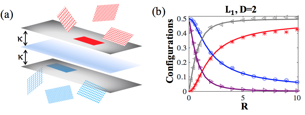
Figure 12: $L_{1}$ balls: (a) Linear classification of 2-$D$ $L_{1}$ balls. (b) Fraction of manifold configurations as a function of radius $R$ at capacity with $\kappa=0$ comparing theory (lines) to simulations (markers). (red) entire manifold embedded, (blue) manifold touching margin at a single vertex, (gray) manifold touching with two corners (one side), (purple) interior manifold.

Discussion:

We have extended Gardner’s theory of the linear classification of isolated points to the classification of continuous manifolds. Our analysis shows how linear separability of the manifolds depends intimately upon the dimensionality, size and shape of the convex hulls of the manifolds. Some or all of these properties are expected to differ at different stages in the sensory hierarchy. Thus, our theory enables systematic analysis of the degree to which this reformatting enhances the capacity for object classification at the higher stages of the hierarchy.

We focused here on the classification of fully observed manifolds and have not addressed the problem of generalization from finite input sampling of the manifolds. Nevertheless, our results about the properties of maximum margin solutions can be readily utilized to estimate generalization from finite samples. The current theory can be extended in several important ways. Additional geometric features can be incorporated, such as non-uniform radii for the manifolds as well as heterogeneous mixtures of manifolds. The influence of correlations in the structure of the manifolds as well as the effect of sparse labels can also be considered. The present work lays the groundwork for a computational theory of neuronal processing of objects, providing quantitative measures for assessing the properties of representations in biological and artificial neural networks.

Appendix

Perceptron Capacity of Line Segments.

The simplest example of linear separability of manifolds is when the manifolds are line segments. Specifically,

we consider the problem of classification of $P$ line segments of length $2R$, given by

$$\left\{\mathbf{x}_{0}^{\mu}+Rs\mathbf{u}^{\mu}\right\},\>|s|\leq 1,\>\mu=1,...P$$ (25)

the $N-$dimensional vectors $\mathbf{x_{0}}^{\mu}$ and $\mathbf{u}^{\mu}$, which are, respectively, the centers and the directions of the $\mu$ segment. [We use the boldface style to denote $N$-dim vectors]. We consider random line segments, specifically assume that the components of all $\mathbf{x_{0}}^{\mu}$ and $\mathbf{u}^{\mu}$ are i.i.d. normally distributed (with zero mean and unit variance). The target classification labels of the manifolds are $y^{\mu}=\pm 1$ and are drawn randomly with equal probability of $\pm 1.$

We search for an $N$-dimenional weight vector $\mathbf{w}$ that classifies correctly the line segments. Since the line segments are convex this is equivalent to the requirement that $\mathbf{w}$ classifies correctly the end points of each segments, This condition can be written using two local fields for each segment. One is the field induced by the center of the line $x^{\mu},$ giving

$$h_{0}^{\mu}=||\mathbf{w}||^{-1}y^{\mu}\mathbf{w}\cdot\mathbf{x_{0}}^{\mu}$$ (26)

The other is the field induced by the direction vector $\mathbf{u}^{\mu},$

$$h^{\mu}=||\mathbf{w}||^{-1}y^{\mu}\mathbf{w}\cdot\mathbf{u}^{\mu}$$ (27)

Note that all the fields are defined with the target label $y^{\mu}$, and they are normalized by the norm of $\mathbf{w}$. With these definitions, $h_{0}^{\mu}\pm Rh^{\mu}$ are the signed distance of the endpoints of the segment from the separating plane which is the plane orthogonal to $\mathbf{w}$ . Thus, $\mathbf{w}$ has to obey,

$$h_{0}^{\mu}-R\left\|h_{i}^{\mu}\right\|\geq\kappa$$ (28)

where $h_{0}^{\mu}-R\left\|h_{i}^{\mu}\right\|$ is the field of the endpoint with the smallest (signed) distance to the plane. The parameter $\kappa>0$ is a parameter defining two margin planes. According to Eq. (28) all the positively labeled inputs must lie either above the ’positive’ margin plane. Conversely the negatively labeled points must lie below the negative margin plane (See Fig. 1).

Replica Theory

We consider a thermodynamic limit where $N,\,P\rightarrow\infty$ whereas $\alpha=P/N$, and $R$ are finite. We use the Gardner framework to compute the volume of space of solutions.

$$V=\int d^{N}\mathbf{w_{\alpha}}\delta(\mathbf{w}^{2}-N)\Pi_{\mu=1}^{P}\Theta(h_{0}^{\mu}-R\left\|h^{\mu}\right\|-\kappa)$$ (29)

where $\Theta$ is the Heaviside function. According to replica theory, $\langle\ln V\rangle=\lim_{n\rightarrow 0}\frac{\langle V^{n}\rangle-1}{n}$, where $V^{n}$ can be written as,

$$V^{n} = \prod_{\alpha=1}^{n}\int d\mathbf{w}_{\alpha}\delta(\mathbf{w}_{\alpha}^{2}-N)\prod_{\mu=1}^{P}\int_{\kappa}^{\infty}dh_{\alpha}^{\mu+}\int_{\kappa}^{\infty}dh_{\alpha}^{\mu-}\int_{-\infty}^{\infty}d\tilde{h}_{\alpha}^{\mu+}\int_{-\infty}^{\infty}d\tilde{h}_{\alpha}^{\mu-}X$$ (30)

$$X=e^{\sum_{\pm}i\tilde{h}_{\alpha}^{\mu\pm}\left(h_{\alpha}^{\mu\pm}-\frac{1}{\sqrt{N}}\left\{y^{\mu}\mathbf{w}_{\alpha}^{T}(\mathbf{x_{0}}^{\mu}\pm R\mathbf{u}^{\mu})\right\}\right)}$$ (31)

where $h^{\mu+}=h_{0}^{\mu}+Rh^{\mu}$, $h^{\mu-}=h_{0}^{\mu}-Rh^{\mu}$. Averaging over the random inputs $\mathbf{x}^{\mu}$ and $\mathbf{u}^{\mu}$ , the above fields can be written as sums of two random fields, where $t_{0}$ and $t$ are the quenched component resulting from the quenched random variables, namely the input vectors $\mathbf{x}_{0}^{\mu}$and $\mathbf{u}_{i}^{\mu}$, while the $z_{0}$and $z$ fields represent the variability of different $\mathbf{w}$’s within the volume of solutions for each realization of inputs and labels,

$$h_{0}^{\mu}=\sqrt{q}t_{0}^{\mu}+\sqrt{1-q}z_{0}^{\mu},\;h^{\mu}=\sqrt{q}t^{\mu}+\sqrt{1-q}z^{\mu}$$ (32)

where the replica symmetric order parameter $q$ is $q=\frac{1}{N}\mathbf{w}_{\alpha}\cdot\mathbf{w}_{\beta},\,\alpha\neq\beta$ . The resultant ’free energy’ $G$ is:

$$\langle V^{n}\rangle_{t_{0},t}=e^{Nn\left[G(q)\right]}=e^{Nn\left[G_{0}(q)+\alpha G_{1}(q)\right]}$$ (33)

where,

$$G_{0}(q)=\frac{1}{2}\ln(1-q)+\frac{q}{2(1-q)}$$ (34)

is the entropic term representing the volume of $\mathbf{w}_{\alpha}$ subject to the constraint that $q=\frac{1}{N}\mathbf{w}_{\alpha}\cdot\mathbf{w}_{\beta}$ . The classification constraints contributes

$$G_{1}(q)=\langle\mbox{ln}Z(q,t_{0,}t)\rangle_{t_{0},t}$$ (35)

$$Z(q,t_{0},t)=\int_{-\infty}^{\infty}Dz_{0}\int_{-\infty}^{\infty}Dz\Theta\left[\left(\sqrt{q}t_{0}+\sqrt{1-q}z_{0}\right)-R\left|\sqrt{q}t+\sqrt{1-q}z\right|-\kappa\right]$$ (36)

where $Dx\equiv\frac{dx}{\sqrt{2\pi}}\exp-\frac{x^{2}}{2}$ and the average wrt $t_{0}$, $t$ denotes integrals over the gaussian variables $t_{0}$, $t$ with measures $Dt_{0}$ and $Dt$, respectively. Finally, $q$ is determined by solving $\frac{\partial G}{\partial q}=0$ . Solution with $q<1$ indicates a finite volume of solutions. For each $\kappa$ there is a maximum value of $\alpha$ where a solution exists. As $\alpha$ approaches this maximal value, $q\rightarrow 1$ indicating the existence of a unique solution, which is the max margin solution for this $\alpha$.

In this chapter we focus on the properties of the max margin solution, i.e., on the limit $q\rightarrow 1.$

$q\rightarrow 1$ Limit

We define

$$Q=\frac{q}{1-q}$$ (37)

and study the limit of $Q\rightarrow\infty$. In this limit the leading order is $G_{0}=\frac{Q}{2}$.

$$\langle\ln V\rangle=\frac{Q}{2}\left[1-\alpha\langle g(t_{0},t)\rangle_{t_{0},t}\right]$$ (38)

where, $g\equiv-\frac{2}{Q}\log Z$ is independent of $Q$ and is given by replacing the integrals in Eq. (171) by their saddle point, yielding

$$g(t_{0},t)=\min_{z_{0}+t_{0}-R|z+t|\geq\kappa}[z_{0}{}^{2}+z^{2}]$$ (39)

Note that here we have scaled variables $z_{0}$ and $z$ such that $z_{0}\rightarrow\sqrt{Q}z_{0}$ and similarly for $z$.

Finally, at the capacity, $\ln V$ vanishes, hence

$$\alpha_{1}^{-1}(\kappa,R)=\langle g(t_{0},t)\rangle_{t_{0},t}$$ (40)

where we have denoted the capacity for one dimensional manifolds as $\alpha_{1}$.

Capacity

The nature of solution of Eq. (39) depends on the values of $t$ and $t_{0}$. There are three regimes.

a) Regime 1:

$$t_{0}-\kappa>R\left\|t\right\|$$ (41)

in which case the solution is $z_{0}=z=0$ which does not contribute to Eq. (40).

For values of $t_{0}-\kappa\leq R||t||$, the solution obeys $z_{0}+t_{0}-R||z+t||=\kappa$ , meaning that one of the endpoints touches the margin plane. This regime is further divided into two cases.

b) Regime 2: $$-R^{-1}||t||<t_{0}-\kappa<R||t||$$ (42)

Here, the center field $z_{0}+t_{0}$ is larger than the margin (i.e., the center points are interior) and the fields can be determined by minimizing Eq. (39) $(R|z+t|-t_{0}+\kappa)^{2}+z^{2}$ w.r.t. $z$ yielding

$$z=\frac{R^{2}||t||+R(\kappa-t_{0})}{1+R^{2}}$$ (43)

$$z_{0}=\frac{R||t||+\kappa-t_{0}}{1+R^{2}}$$ (44)

and its contribution to Eq. (40) is

$$g=\frac{(\kappa-t_{0}+R||t||)^{2}}{1+R^{2}}$$ (45)

c) Regime 3: $$t_{0}-\kappa<-R^{-1}||t||$$ (46)

Here the center points are also on the margin plane, hence $z=-||t||$ and $z_{0}+t_{0}=\kappa$, contributing

$$g=(t_{0}-\kappa)^{2}+t^{2}$$ (47)

Finally, combining the contributions from Regimes 2 and 3 yields,

$$\alpha_{L}^{-1}(\kappa,R)=\int_{-\infty}^{\infty}Dt\left[\int_{\kappa-|t|R^{-1}}^{\kappa+R|t|}Dt_{0}\frac{(|t|R-(t_{0}-\kappa))^{2}}{(1+R^{2})}+\int_{-\infty}^{\kappa-|t|R^{-1}}Dt_{0}((t_{0}-\kappa)^{2}+t^{2})\right]$$ (48)

For $\kappa=0$, this expression reduces to

$$\alpha_{L}^{-1}(0,R)=\int_{-\infty}^{\infty}Dt\left[\int_{-|t|R^{-1}}^{R|t|}Dt_{0}\frac{(|t|R-t_{0})^{2}}{(1+R^{2})}+\int_{-\infty}^{-|t|R^{-1}}Dt_{0}(t_{0}^{2}+t^{2})\right]$$ (49)

By switching to polar coordinates: $t=r\cos\phi$, $t_{0}=r\sin\phi,$ these integrals reduce to

$$\alpha_{L}^{-1}(R)=\frac{1}{2}+\frac{2}{\pi}\arctan R$$ (50)

Limits of R

In the limit of $R\rightarrow 0,$ Eq. (48) reduces to $\alpha_{L}(\kappa,R=0)=\alpha_{0}(\kappa)$ where $\alpha_{0}(\kappa)$ is the Gardner’s result for classifying $P$ random points.

Interestingly, $\alpha_{L}(\kappa,1)=\frac{1}{2}\alpha_{0}(\kappa/\sqrt{2})$ . This is because when $R=1$ the distance between edge points on the line segments is statistically the same as that between points of different segments, hence the problem is equivalent to classifying randomly $2P$ points with norms $\sqrt{2N}$.

Finally, when $R\rightarrow\infty,$ the capacity becomes

$$\alpha_{L}^{-1}(\kappa,R=\infty)=\int_{-\infty}^{\infty}Dt\left[\int_{\kappa}^{\infty}Dt_{0}t^{2}+\int_{-\infty}^{\kappa}Dt_{0}((t_{0}-\kappa)^{2}+t^{2})\right]$$ (51)

$$=1+\int_{-\infty}^{\kappa}Dt_{0}((t_{0}-\kappa)^{2}=1+\alpha_{0}^{-1}(\kappa)$$ (52)

The reason for this is that when $R$ is large, the manifolds are essentially unbounded lines. The only way to classify them correctly is for $\mathbf{w}$ to be orthogonal to all $P$ lines, reducing the problem to classifying $P$ points which are the projections of the centers on the null space of the lines. Thus, this is equivalent to classifying random points in a space with dimensionality $N-P=N(1-\alpha)$ from which Eq. (51) follows. These limits can be readily seen in the simple case of $\kappa=0$. It is readily seen from Eq. (50) that $\alpha=2$, $1,$ and $2/3$ for $R=0,$1, and $\infty$ respectively.

Distribution of Fields

It is instructive to calculate the distribution of fields $P(h_{0},h)$ induced by the manifolds with the max margin solution $\mathbf{w}$. Using the above theory, we find that

$$P(h_{0},h) = \langle\frac{1}{Z}\int_{-\infty}^{\infty}Dz_{0}\int_{-\infty}^{\infty}Dz\Theta\left[\left(\sqrt{q}t_{0}+\sqrt{1-q}z_{0}\right)-R\left|\sqrt{q}t+\sqrt{1-q}z\right|-\kappa\right]$$ (54)

$$\delta(h_{0}-\sqrt{q}t_{0}-\sqrt{1-q}z_{0})\delta(h-\sqrt{q}t-\sqrt{1-q}z)\rangle_{t,t_{0}}$$

Considering the three above regimes for $(t,t_{0})$, we obtain the dominant contribution in the limit of $Q\rightarrow\infty$,

$$P(h_{0},h)=A(h_{0},h)\Theta(h_{0}-R||h||-\kappa)+B(h_{0})\delta(||h||-R^{-1}(h_{0}-\kappa))+C\delta(h_{0}-\kappa)\delta(h)$$ (55)

$$A(h_{0},h)=\frac{\exp(-\frac{1}{2}(h_{0}^{2}+h^{2})}{2\pi},\,h_{0}-R|h|-\kappa\geq 0$$ (56)

$$B(h_{0})=2\sqrt{\frac{1+R^{-2}}{2\pi}}H(-R^{-1}\kappa^{\prime})\exp\left[-\frac{(1+R^{-2})(h_{0}-R^{-2}\kappa^{\prime})^{2}}{2}\right],\,h_{0}\geq 0$$ (57)

$$C=\int Dz\int_{-\infty}^{\kappa-R^{-1}||z||}Dt$$ (58)

where $H(x)=\int_{x}^{\infty}Dz$ , and

$$\kappa^{\prime}=\frac{\kappa}{1+R^{-2}}$$ (59)

The integrated weights are:

$$\int dh_{0}dhA(h_{0},h)=2\int_{0}^{\infty}DtH(\kappa+Rt)$$ (60)

$$\int dh_{0}B(h_{0})=\int_{-\infty}^{\infty}Dt\int_{\kappa-|t|R^{-1}}^{\kappa+R|t|}Dt_{0}=2\int_{0}^{\infty}Dt\left[H(\kappa-tR^{-1})-H(\kappa+Rt)\right]$$ (61)

$$C=\int_{-\infty}^{\infty}Dt\int_{-\infty}^{\kappa-|t|R^{-1}}Dt_{0}=1-2\int_{0}^{\infty}DtH(\kappa-tR^{-1})$$ (62)

The first term represents the fraction of line segments that are interior to the margin plane (corresponding to Regime 1); the second component corresponds to segments that touch the margin planes but do not lie on the margin plane (Regime 2); the third term corresponds to the segments that lie completely on the margin planes (see Fig. 1 in main text). When $R\rightarrow\infty,$ we obtain,

$$\int dh_{0}B(h_{0})=H(\kappa)$$ (63)

$$C=1-H(\kappa)$$ (64)

The reason for this is as follows. when $R\rightarrow\infty$, $\mathbf{w}$ becomes increasingly orthogonal to all the directors, hence the fraction of interior points vanish. The value of $B$ represents the fraction of segments that touch the margin planes. The fields associated with the centers is finite, larger than $\kappa$. However, the angle between the segments and $\mathbf{w}$ vanish, since the angle is roughly $||h||$ which is $R^{-1}(h_{0}-\kappa)$ . In contrast, the fields of the segments represented by $C$ equal $\kappa$, hence they lie in the margin planes. Thus, in this limit, the fields are the same as the separation of the centers in the null space (of dimension $N-P)$.

Perceptron Capacity of $D$-dimensional Balls

We now consider linear classification of higher dimensional manifolds, modeling them as $D$ dimensional balls with radius $R$,

$$\mathbf{x_{0}}^{\mu}+R\sum_{i=1}^{D}s_{i}\mathbf{u}_{i}^{\mu},\>\forall s,\>||\vec{s}||\leq 1$$ (65)

[We use $\vec{}\>$ sign to denote $D$ - dimensional vectors and $||...||$ for $L_{2}$ norm ]. For each manifold, the center $\mathbf{x}_{0}^{\mu}$, and the $D$ basis vectors $\{\mathbf{u}_{i}^{\mu}\}$ are $N$ dimensional vectors ($i=1,..,D$), the components of which are all independent Gaussian random variables with zero mean and unit variance. The target labels of the manifolds are random assignments of $y^{\mu}=\pm 1$. To classify all the points on the manifolds correctly (with a given margin), the weight vector $\mathbf{w}$ (normalized for convenience by $||\mathbf{w}||=\sqrt{N}),$ must satisfy

$$h_{0}^{\mu}+R\min_{\vec{s},\,||\vec{s}||^{2}=1}\sum_{i=1}^{D}s_{i}h_{i}^{\mu}\geq\kappa$$ (66)

where $h_{0}^{\mu}=N^{-1/2}y^{\mu}\mathbf{w}\cdot\mathbf{x^{\mu}}$ is the field induced by the manifold centers and $h_{i}^{\mu}=N^{-1/2}y^{\mu}\mathbf{w}\cdot\mathbf{u}_{i}^{\mu}\>i=1,...,D$ are $D$ fields induced by each of the basis vectors. Differentiating $\sum_{i=1}^{D}s_{i}h_{i}^{\mu}+\lambda\sum_{i}s_{i}^{2}$ (where $\lambda$ is a Lagrange multiplier enforcing the norm constraint) wrt $s_{i}$, we obtain,

$$s_{i}=-\frac{h_{i}^{\mu}}{||\vec{h}^{\mu}||}$$ (67)

where $||\vec{h}^{\mu}||$ is the $L_{2}$ norm of the $D$-dimensional vector $h_{i}^{\mu}$, hence $\sum_{i}s_{i}h_{i}^{\mu}=-||\vec{h}^{\mu}||$ and the constraints can be written as

$$h_{0}^{\mu}-R||\vec{h}^{\mu}||\geq\kappa$$ (68)

Geometrically, the LHS corresponds to the field induced by the point on the manifold $\mu$ which has the smallest (signed) projection on $\mathbf{w}$. We consider a thermodynamic limit where $N,\,P\rightarrow\infty$ while $\alpha=P/N$, $D,$ and $R$ are finite.

Capacity

The replica theory as outlined above, yields

$$\langle V^{n}\rangle_{t_{0},t}=e^{Nn\left[G(q)\right]}=e^{Nn\left[G_{0}(q)+\alpha G_{1}(q)\right]}$$ (69)

where as before,

$$G_{0}(q)=\frac{1}{2}\ln(1-q)+\frac{q}{2(1-q)}$$ (70)

and

$$G_{1}(q)=\langle\ln Z(q,t_{0,}\vec{t})\rangle_{t_{0},\vec{t}}$$ (71)

$$Z(q,t_{0},\mathbf{t})=\int_{-\infty}^{\infty}Dz_{0}\int_{-\infty}^{\infty}D\vec{z}\Theta\left[\left(\sqrt{q}t_{0}+\sqrt{1-q}z_{0}\right)-R||\sqrt{q}\vec{t}+\sqrt{1-q}\vec{z}||-\kappa\right]$$ (72)

where

$$h_{0}^{\mu}=\sqrt{q}t_{0}^{\mu}+\sqrt{1-q}z_{0}^{\mu},\;h_{i}^{\mu}=\sqrt{q}t_{i}^{\mu}+\sqrt{1-q}z_{i}^{\mu},\,i=1,...,D$$ (73)

and $||...||$ is the $L_{2}$ norm of the $D$-dimensional vectors. All variables $z_{0},t_{0},\vec{z},\vec{t}$ are normally distributed.

$$\ln Z(q,t_{0},\vec{t})=\ln\int_{-\infty}^{\infty}Dz_{0}\int_{-\infty}^{\infty}D\vec{z}\,\Theta\left(\sqrt{Q}t_{0}+z_{0}-R||\sqrt{q}\vec{t}+\sqrt{1-q}\vec{z}||-\kappa\right)$$

where the saddle point behavior in the limit of $q\rightarrow 1,Q\rightarrow\infty$ gives $g\equiv-\frac{2}{Q}\log Z$,

$$g(t_{0,}t)=\min_{t_{0}+z_{0}-R||\vec{t}+\vec{z}||>\kappa}\frac{1}{2}\left[z_{0}^{2}+\left\|\vec{z}\right\|^{2}\right]$$ (74)

and the capacity is given by

$$\alpha_{B}^{-1}(\kappa,R,D)=\langle g(t_{0},\vec{t})\rangle_{t_{0},\mathbf{\vec{t}}}$$ (75)

Again, there are three regimes.

a) Regime 1:

Defining $t=||\vec{t}||$, when $t_{0}-\kappa>Rt$: then $z_{0}\approx 0$, $\vec{z}\approx 0$ $g\approx 0$ corresponding to manifolds which obey the inequality (not equality) of Eq. (162), hence are interior to the plane.

b) Regime 2:

When $-R^{-1}t<t_{0}-\kappa<Rt$: then $z_{0}=R||\vec{t}+\vec{z}||-t_{0}+\kappa$ and

$$\vec{z}=-z\vec{t}/t$$ (76)

the scalar $z$ can be calculated by

$$g\approx\min_{z}\frac{1}{2}\left[\left(R(t-z)-t_{0}+\kappa\right)^{2}+z^{2}\right]$$ (77)

$$z=\frac{R^{2}t-R(\kappa-t_{0})}{1+R^{2}}$$ (78)

$$z_{0}=\frac{Rt+\kappa-t_{0}}{1+R^{2}}$$ (79)

$$g=\frac{(\kappa-t_{0}-Rt)^{2}}{1+R^{2}}$$ (80)

c) Regime 3:

When $t_{0}<-\frac{1}{R}t$: then $z=t$ and $z_{0}=\kappa-t_{0}$ so that $g\approx(t_{0}-\kappa)^{2}+t^{2}$ .

Combining these contributions, the capacity is:

$$\alpha_{B}^{-1}(\kappa,R,D)=\int_{0}^{\infty}dt\chi{}_{D}(t)\left[\int_{\kappa-\frac{1}{R}t}^{\kappa+Rt}Dt_{0}\frac{(Rt-t_{0}+\kappa)^{2}}{R^{2}+1}+\int_{-\infty}^{\kappa-\frac{1}{R}t}Dt_{0}([t_{0}-\kappa]^{2}+t^{2})\right]$$ (81)

where $\chi_{D}$ is the $D$-dim Chi distribution,

$$\chi_{D}(t)=\int D\vec{t}\delta\left(t-||\vec{t}||\right)=\frac{2^{1-\frac{D}{2}}t^{D-1}e^{-\frac{1}{2}t^{2}}}{\Gamma(\frac{D}{2})}$$ (82)

Distribution of Fields

We consider the joint distribution of two fields: $h_{0}$ which is the field induced by the manifold centers, and $h\equiv||\vec{h}||$, namely the $L_{2}$ norm of the $D$ dimensional vector of fields induced by the $D$ $\mathbf{u}_{i}$’s. Taking into account the above three regimes, we have,

$$P(h_{0},h)=A(h_{0},h)\Theta(h_{0}-Rh-\kappa)+B(h_{0})\delta(h-R^{-1}(h_{0}-\kappa))+C\delta(h_{0}-\kappa)\delta(h)$$ (83)

1. Field Distribution for $\kappa=0$.

$$A(h_{0},h)=\frac{\exp(-\frac{1}{2}h_{0}^{2})}{\sqrt{2\pi}}\chi_{D}(h),\,h_{0}-R|\vec{h}|\geq 0$$ (84)

$$B(h_{0})=(1+R^{2})^{-1}\int Dt_{0}\int_{h}^{\infty}dt\chi_{D}(t)\,\delta(t_{0}-(1+R^{-2})h_{0}-R^{-1}t)$$ (85)

$$C=\int Dz\int_{-\infty}^{\kappa-R^{-1}|\vec{z}|}Dt$$ (86)

2. Integrated Weights:

$$\int dh_{0}dhA(h_{0},h)=\int_{0}^{\infty}dtP_{D}(t)H(\kappa+Rt)$$ (87)

$$\int dh_{0}B(h_{0})=\int_{0}^{\infty}dt\chi_{D}(t)\int_{\kappa-\frac{1}{R}t}^{\kappa+Rt}Dt_{0}=\int_{0}^{\infty}dt\chi_{D}(t)\left[H(\kappa-\frac{t}{R})-H(\kappa+Rt)\right]$$ (88)

$$C=\int_{0}^{\infty}dt\chi_{D}(t)\int_{-\infty}^{\kappa-\frac{t}{R}}Dt_{0}=1-\int_{0}^{\infty}dt\chi_{D}(t)H(\kappa-\frac{t}{R})$$ (89)

As in the case of line segments, the first term corresponds to the fraction of $D$-dim balls that lie in the interior space; the second component corresponds to the fraction of balls that touch the margin planes, whereas $C$ stands for the fraction of balls that are fully embedded in these planes.

$R=1$

1. Capacity for $\kappa=0$

In the case of $R=1$, the capacity obtains a simple form:

$$\alpha_{B}^{-1}(\kappa=0,R=1,D)=\int_{0}^{\infty}dt\chi{}_{D}(t)\left[\int_{-t}^{+t}Dt_{0}\frac{t^{2}+t_{0}^{2}}{2}-\int_{-t}^{+t}Dt_{0}tt_{0}+\int_{-\infty}^{-t}Dt_{0}(t_{0}{}^{2}+t^{2})\right]$$

$$\alpha_{B}^{-1}(\kappa=0,R=1,D)=\int_{0}^{\infty}dt\chi{}_{D}(t)\left[\int_{0}^{\infty}Dt_{0}(t_{0}{}^{2}+t^{2})\right]$$

$$\alpha_{B}^{-1}(\kappa=0,R=1,D)=\frac{D+1}{2}\>\square$$

2. Manifold Geometry Configurations for $\kappa=0$

a) Interior vs. Embedded:

The fraction of embedded manifolds:

$$p_{\mbox{embedded}}=\int_{0}^{\infty}dt\chi{}_{D}(t)\left[\int_{-\infty}^{-t}Dt_{0}\right]$$

Fraction of interior manifolds:

$$p_{\mbox{interior}}=\int_{0}^{\infty}dt\chi{}_{D}(t)\int_{t}^{\infty}Dt_{0}=p_{\mbox{embedded}}$$

The fraction of touching manifolds:

$$p_{\mbox{touching}}=\int_{0}^{\infty}dt\chi{}_{D}(t)\int_{-t}^{t}Dt_{0}$$

Thus, the fraction of interior manifolds and embedded manifolds are equal. $\square$.

b) Touching Manifolds:

In general,

$$p_{\mbox{touching}}=\int_{0}^{\infty}dt\chi{}_{D}(t)\left[\int_{-\frac{1}{R}t}^{+Rt}Dt_{0}\right]$$

$$=\int_{0}^{\infty}dt\chi{}_{D}(t)\left[1-H(Rt)-H(t/R)\right]$$

The radius $R$ at which $p_{\mbox{touching}}$is at maximum can be found by

$$\frac{\partial}{\partial R}\left(p_{\mbox{touching}}\right)=\int_{0}^{\infty}dt\chi{}_{D}(t)\left[-tH^{\prime}(Rt)+tR^{-2}H^{\prime}(t/R)\right]=0$$

The solution for above is $R=1$ for all $D$. For $D=2$ , $p_{\mbox{touching}}(R=1,D=2)=\int_{0}^{\infty}dt\chi_{2}(t)[1-2H(t)]\sim 0.7$.

Therefore, at $R=1$, the fraction of touching disks is at maximum, and for $D=2$, the value is about 0.7. $\square.$

Large $R$ Limit

In the limit of large $R$, Eq. (81) reduces to:

$$\alpha_{B}^{-1}(\kappa,R=\infty,D)=\int_{0}^{\infty}dt\chi{}_{D}(t)\left[\int_{\kappa}^{\infty}Dt_{0}t^{2}+\int_{-\infty}^{\kappa}Dt_{0}([t_{0}-\kappa]^{2}+t^{2})\right]$$ (90)

$$=\int_{0}^{\infty}dt\chi{}_{D}(t)t^{2}+\int_{-\infty}^{\kappa}Dt_{0}(t_{0}-\kappa)^{2}=\alpha_{0}^{-1}(\kappa)+D$$ (91)

which reflects the fact that when $R$ is large $\mathbf{w}$ must be in the null space of the $PD$ vectors $\mathbf{u}_{i}^{\mu}$; thus, the classification problem is that of $P$ points (i.e., the projections of the centers onto the null space) in $N-PD$ dimensions. Likewise, in this limit $A$ vanishes and the angle between the manifold centers and the margin planes vanish.

Limit of Large $D$

In many realistic problems it is expected that the dimension of the object manifolds is large, hence it is of interest to examine the results in the limit of $D\gg 1$. In his limit, $\chi_{D}(t)$ is centered around $t=\sqrt{D}$, yielding

$$\alpha_{B,D\gg 1}^{-1}=\int_{\kappa-\frac{\sqrt{D}}{R}}^{\kappa+R\sqrt{D}}Dt_{0}\frac{(R\sqrt{D}-t_{0}+\kappa)^{2}}{R^{2}+1}+\int_{-\infty}^{\kappa-\frac{\sqrt{D}}{R}}Dt_{0}([t_{0}-\kappa]^{2}+D)$$ (92)

As long as $R\ll\sqrt{D}$ , the second term in Eq. (92) vanishes and yields

$$\alpha_{B,D\gg 1}^{-1}=\int_{-\infty}^{\kappa+R\sqrt{D}}Dt_{0}\frac{(R\sqrt{D}-t_{0}+\kappa)^{2}}{R^{2}+1}=\frac{\alpha_{0}^{-1}(\kappa+R\sqrt{D})}{1+R^{2}}$$ (93)

Thus, $\alpha$remains finite in the limit of large $D$ only if $R$ is not larger than the order of $D^{-1/2}$. If, on the other hand, $R\sqrt{D}\gg 1$, Eq. (93) implies

$$\alpha_{B,D\gg 1}^{-1}=\frac{R^{2}D}{1+R^{2}}$$ (94)

(where we have used the asymptote $\alpha_{0}^{-1}(x)\rightarrow x$ for large $x$).

Numerically, this approximation works very well for $R\geq 0.5$ and all $D$ (as long as $R\ll\sqrt{D}$).

Field Distribution in Large $D$ :

In the limit of large $D$ , the fraction of manifolds that lie on the margin plane, $C$, is zero. The overall fraction of interior manifolds is $H(\kappa+R\sqrt{D})$ whereas the fraction of manifolds that touch the margin planes is $1-H(\kappa+R\sqrt{D})$ .

Large $R$ :

In the limit of $R\propto\sqrt{D}$,

$$\alpha_{B,R\gg 1}^{-1}=D\int_{\kappa-\frac{\sqrt{D}}{R}}^{\infty}Dt_{0}+D\int_{-\infty}^{\kappa-\frac{\sqrt{D}}{R}}Dt_{0}=D$$ (95)

Note that in this case, both terms in Eq. (92) contribute. This reflects the fact that when $R$ is $O(\sqrt{D})$ it is again advantageous for $\mathbf{w}$ to be orthogonal to some of the spheres. This is seen in the field distribution. In this limit, it consists of a fraction of $H(\sqrt{D}/R)$ lying on the plane whereas the fraction of touching balls is $1-H(\sqrt{D}/R)$. Finally, when $R/\sqrt{D}$ is large, most of the spheres lie on the margin, as expected.

Perceptron Capacity of $L_{p}$ Manifolds

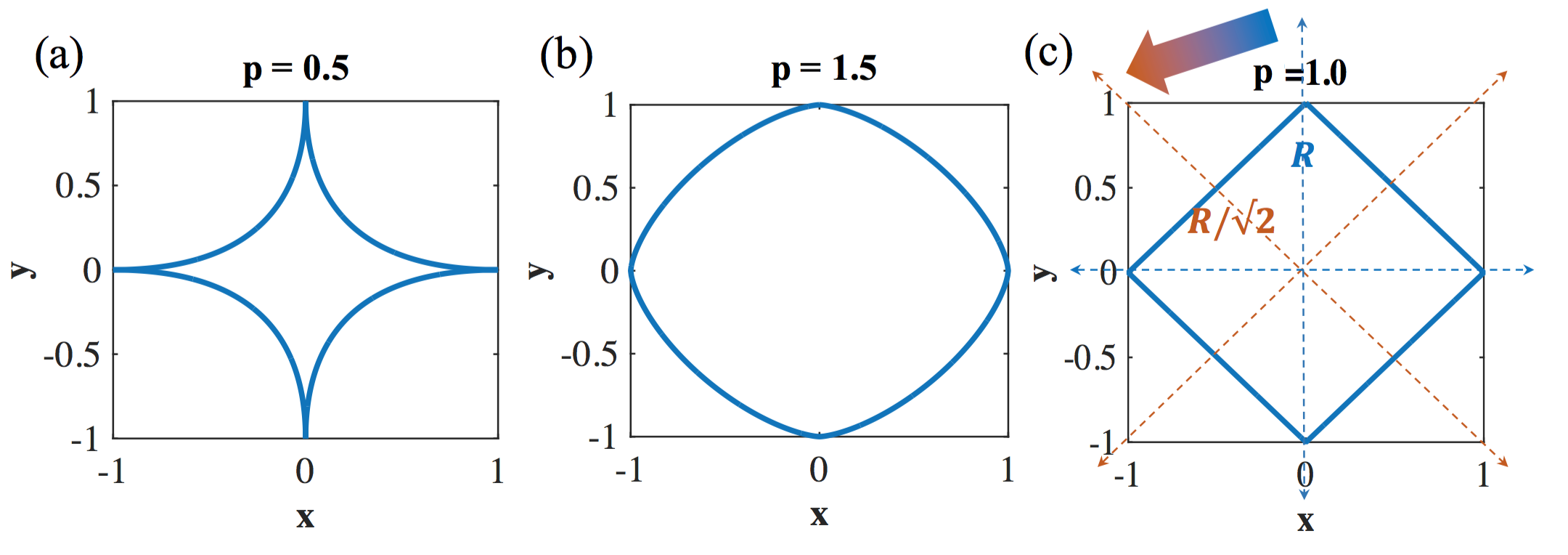
Figure 13: $L_{p}$ balls. Illustration of $L_{p}$ balls of norm $p$ for (a) $p$ = 0.5, (b) $p$ =1.5, (c) $p$ = 1. Notice that rotation of the axis introduces the reduction of effective $R$ by factor of $1/\sqrt{2}$.

We consider manifolds defined with $L_{p}$ norm,

$$\mathbf{x_{0}}^{\mu}+R\sum_{i=1}^{D}s_{i}\mathbf{u}_{i}^{\mu},\>\forall s,\>\left\|\vec{s}\right\|_{p}\leq 1$$ (96)

where $\vec{\left\|s\right\|}{}_{p}$ is the $L_{p}$norm of $\vec{s}$ . Linear classification requires

$$h_{0}^{\mu}+R\min_{s,\,\left\|\vec{s}\right\|_{p}=1}\sum_{i=1}^{D}s_{i}h_{i}^{\mu}\geq\kappa$$ (97)

$1<p<\infty$:

Differentiating $\sum_{i}s_{i}h_{i}^{\mu}+\lambda\sum_{i}\left\|s_{i}\right\|{}^{p}$ wrt $s_{i}$ yields,

$$s_{i}=-\mbox{sign}(h_{i}^{\mu})\frac{||h_{i}^{\mu}||^{1/(p-1)}}{(||h^{\mu}||_{q})^{1/p}}$$ (98)

where $q=\frac{p}{p-1}$ is the dual norm of $p$ , hence, $\min_{\vec{s},\,\vec{\left\|s\right\|}_{p}=1}\sum_{i=1}^{D}s_{i}h_{i}^{\mu}=-\left\|\vec{h}^{\mu}\right\|{}_{q}$ . Thus, linear classification of $L_{p}$ manifolds is equivalent to the constraints on the fields,

$$h_{0}^{\mu}-R\left\|\vec{h}^{\mu}\right\|{}_{q}\geq\kappa$$ (99)

Smoothness of the $L_{q}$ norm guarantees that the solution will be qualitatively similar to spheres (i.e., $p=q=2$). (See Fig. 13(a) in the Appendix)

$0<p\leq 1$:

In this regime differentiating with respect to $s_{i}$ does not minimize $\sum_{i}s_{i}h_{i}^{\mu}$ . Instead, the minima are at the $D$ extremal points: $s_{i}=1,\,s_{j}=0,\,j\neq i$ corresponding to the corners of the manifolds (see Fig. 13(b)). Thus, for all $p\leq 1$ the linear classification constraint is the same and is given by the corner with the smallest projection on $w$ , namely

$$h_{0}^{\mu}-R\max_{i}h_{i}^{\mu}\geq\kappa$$ (100)

We can now use the replica theory, where now the capacity is given by

$$\alpha_{B_{p}}^{-1}(\kappa,R,D)=\langle g(t_{0},\vec{t})\rangle_{t_{0},\vec{t}}$$ (101)

where $B_{p}$ stands for Balls with $L_{p}$ norm,

$$g(t_{0,}t)=\min_{t_{0}+z_{0}-R\max_{i}(z_{i}+t_{i})>\kappa}\frac{1}{2}\left[z_{0}^{2}+\left\|\vec{z}\right\|^{2}\right]$$ (102)

where,

$$z_{0}+t_{0}-R\max_{i}(z_{i}+t_{i})\geq\kappa$$ (103)

$L_{1}$ in $D=2$

Rotated Coordinates

Without loss of generality, we assume the $t_{i}$ are ordered: $t_{2}\geq t_{1}\geq 0$ and similarly for $z_{i}+t_{i}$ .

It is easier to consider the following transformation

$$t_{1}^{\prime}=\frac{1}{\sqrt{2}}(t_{2}-t_{1})$$ (104)

$$t_{2}^{\prime}=\frac{1}{\sqrt{2}}(t_{2}+t_{1})$$ (105)

$$z_{1}^{\prime}=\frac{1}{\sqrt{2}}(z_{2}-z_{1})$$ (106)

$$z_{2}^{\prime}=\frac{1}{\sqrt{2}}(z_{2}+z_{1})$$ (107)

$$R^{\prime}=R/\sqrt{2}$$ (108)

see the geometry of the rotation in Fig. 13 (c).

In these coordinates and convention, $\max_{i}(z_{i}+t_{i})=z_{2}+t_{2}=\frac{1}{\sqrt{2}}\sum_{i}(z^{\prime}_{i}+t^{\prime}_{i})$ hence,

$$g(t_{0,}t)=\min_{t_{0}+z_{0}-R\left\|\vec{z}+\vec{t}\right\|{}_{1}>\kappa}\frac{1}{2}\left[z_{0}^{2}+\left\|\vec{z}\right\|{}^{2}\right]$$ (109)

where we have dropped the primes.

General solution:

$$z=-a,\>a>0$$ (110)

The sign is well defined only for $t+z\neq 0$ . Hence the general solution takes the form

$$z_{i}=-\min(a,t_{i}),\>a\geq 0$$ (111)

a) $t_{0}-\kappa>R||\vec{t}||_{1}:$

$$z_{0},\>z=0$$ (112)

b) $t_{0}-\kappa<R|\vec{t}|_{1}:$

$$z_{0}=\kappa-t_{0}+R|\left\|\vec{z}+\vec{t}\right\|{}_{1}$$ (113)

$$a=\frac{R(R\left\|\vec{t}\right\|{}_{1}-t_{0}+\kappa)}{1+2R^{2}}$$ (114)

$$g=\frac{(R\left\|\vec{t}\right\|{}_{1}-t_{0}+\kappa)^{2}}{(1+2R^{2})}$$ (115)

This is consistent if

$$0<\frac{R(R\left\|\vec{t}\right\|{}_{1}-t_{0}+\kappa)}{1+2R^{2}}<t_{1}$$ (116)

$$t_{0}-\kappa>R\left\|\vec{t}\right\|{}_{1}-R^{-1}(1+2R^{2})t_{1}=t^{1}$$ (117)

$$t_{0}-\kappa>t^{1}$$ (118)

c) $t_{0}<t^{1}$

$$t^{1}=R(t_{1}+t_{2})-R^{-1}(1+2R^{2})t_{1}=R(t_{2}-t_{1})-R^{-1}t_{1}$$ (119)

Assume

$$z_{2}=-a,\>z_{1}=-t_{1},\>t_{2}>a>t_{1}$$ (120)

$$a=\frac{R(Rt_{2}-t_{0}+\kappa)}{1+R^{2}}$$ (121)

$$g=t_{1}^{2}+\frac{(Rt_{2}-t_{0}+\kappa)^{2}}{(1+R^{2})}$$ (122)

$$t_{0}-\kappa>-R^{-1}t_{2}=t^{2}$$ (123)

d) $t_{0}<t^{2}$

$$z=-t$$ (124)

$$g=(t_{0}-\kappa)^{2}+t^{2}$$ (125)

Capacity

Finally, converting back the above regimes and values of $g$ to the original coordinates, we have

$$\alpha_{B_{1}}^{-1}=8\int_{0}^{\infty}Dt_{2}\int_{0}^{t_{2}}Dt_{1}\int_{\kappa+Rt_{1}-R^{-1}(t_{2-}t_{1})}^{\kappa+Rt_{2}}Dt_{0}\frac{(Rt_{2}-t_{0}+\kappa)^{2}}{(1+R^{2})}$$ (126)

$$+8\int_{0}^{\infty}Dt_{2}\int_{0}^{t_{2}}Dt_{1}\int_{\kappa-R^{-1}(t_{1}+t_{2})}^{\kappa+Rt_{1}-R^{-1}(t_{2-}t_{1})}Dt_{0}\left[\frac{(t_{2}-t_{1})^{2}}{2}+\frac{(\frac{1}{2}R(t_{1}+t_{2})-t_{0}+\kappa)^{2}}{(1+\frac{1}{2}R^{2})}\right]$$ (127)

$$+8\int_{0}^{\infty}Dt_{2}\int_{0}^{t_{2}}Dt_{1}\int_{-\infty}^{\kappa-R^{-1}(t_{1}+t_{2})}Dt_{0}\left[(t_{0}-\kappa)^{2}+t_{1}^{2}+t_{2}^{2}\right]$$ (128)

where the subscript for $\alpha_{B_{1}}^{-1}$ is used to denote capacity for balls with $L_{1}$ norm.

1. $R\rightarrow 0$

$$\alpha_{B_{1}}^{-1}=8\int_{0}^{\infty}Dt_{2}\int_{0}^{t_{2}}Dt_{1}\int_{-\infty}^{\kappa}Dt_{0}(-t_{0}+\kappa)^{2}=\alpha_{0}^{-1}(\kappa)$$ (129)

2. $R\rightarrow\infty$

$$\alpha_{B_{1}}^{-1}=8\int_{0}^{\infty}Dt_{2}\int_{0}^{t_{2}}Dt_{1}\int_{\kappa}^{\infty}Dt_{0}\left[\frac{(t_{2}-t_{1})^{2}+(t_{1}+t_{2})^{2}}{2}\right]$$ (130)

$$+8\int_{0}^{\infty}Dt_{2}\int_{0}^{t_{2}}Dt_{1}\int_{-\infty}^{\kappa}Dt_{0}\left[[t_{0}-\kappa]^{2}+t_{1}^{2}+t_{2}^{2}\right]$$ (131)

$$=\int_{-\infty}^{\infty}Dt_{2}\int_{-\infty}^{\infty}Dt_{1}\int_{-\infty}^{\infty}Dt_{0}\left[t_{1}^{2}+t_{2}^{2}\right]+\int_{-\infty}^{\infty}Dt_{2}\int_{-\infty}^{\infty}Dt_{1}\int_{-\infty}^{\kappa}Dt_{0}[t_{0}-\kappa]^{2}$$ (132)

$$\alpha_{B_{1}}^{-1}=2+\alpha_{0}^{-1}(\kappa)$$ (133)

as expected in this case of $D=2$. The effective dimensionality is $N-2P$ .

Fields.

The integrated weight of manifolds that touch the margin planes is

$$8\int_{0}^{\infty}Dt_{2}\int_{0}^{t_{2}}Dt_{1}\int_{\kappa+Rt_{1}-R^{-1}(t_{2-}t_{1})}^{\kappa+Rt_{2}}Dt_{0}$$ (134)

The integrated weight of manifold that have a side on the planes is

$$8\int_{0}^{\infty}Dt_{2}\int_{0}^{t_{2}}Dt_{1}\int_{\kappa-R^{-1}(t_{1}+t_{2})}^{\kappa+Rt_{1}-R^{-1}(t_{2-}t_{1})}Dt_{0}$$ (135)

The fraction of manifolds that lie on the planes is

$$8\int_{0}^{\infty}Dt_{2}\int_{0}^{t_{2}}Dt_{1}\int_{-\infty}^{\kappa-R^{-1}(t_{1}+t_{2})}Dt_{0}$$ (136)

Simulation Details

Linear Classification of Line Segments

Linear Classification of Line Segments.

The classification problem of $P$ line segments is cast in the form of linear classification of the $2P$ endpoints where each pair of endpoints receive the same target label. These labeled inputs were classified using IBM cplex package which uses quadratic programming solving the primal support vector problem. To compute the network capacity $\alpha=P/N$, 100 trials were used for each $P$ and the fraction of converged trials was computed. $P$ was gradually increased. Maximum capacity was defined as the value of $P$ for which the convergence rate reached 0.5. In Fig. 1(c) (main text) $N=200$ was used. To obtain the capacity for $\kappa=0.5$, $P$ was varied until SVM’s maximum margins averaged over $100$ runs was close to $\kappa=0.5$.

Fraction of Line Segment Configurations.

Once the data was determined to be separable, the fraction of the different line segment configurations was computed. Each line segment’s configuration was determined based on the number of endpoints on the main plane. Endpoints were considered to be on the margin plane iff their field was larger than the margin by an amount smaller than a tolerance of $\epsilon=10^{-8}$ .

Linear Classification of D-dimensional $L_{2}$ balls

Sampling of $L_{2}$ balls of Dimension $D$.

Unlike the case of the line segments, where it is sufficient to consider the endpoints, finding SVM solution for classifying $D$ dimensional $L_{2}$ norm balls requires an iterative algorithm to sample the points on the $L_{2}$ balls so that the decision plane is efficiently determined. First, we sample randomly a number of points on all manifolds and find the max margin solution $\mathbf{w}$ and its margin $\kappa$, for this set of points. Next, for each manifold we find analytically the point on the boundary which has the minimum (signed) distance from the decision plane given by $\mathbf{w}$. If the field of this point lies below the margin this point is added to the training data and a new $\mathbf{w}$ is computed. This iterative procedure stops when all the minimal points lie above or on the current margin, guaranteeing the correct classifications of the entire manifolds. For details, see Alg.1.

Initialize:

    $\mathbf{x}^{\mu},\mathbf{\vec{u}}^{\mu}\sim Norm(0,1)$ ( $\mu=1,...,P$) [Sample centers and direction vectors]

    $y^{\mu}\sim\mbox{sign}\left\{\mbox{unif}(-1,1)\right\}$ ( $\mu=1,...,P$) [Sample labels for manifolds]

    $s_{i}^{k}\sim\mbox{unif}\left(-1,1\right)$ and $||\vec{s}^{k}||=1$ $k=1,...,m$. [Sample $m$ coefficient vectors]

    $\mathbf{x}^{\mu}+R\sum_{i=1}^{D}s_{i}^{k}\mbox{{u}}_{i}^{\mu}$$\in D_{\mbox{data}}$ [Construct $m$ points on each manifold]

    t=0; $w_{svm}^{t}=\mbox{svmsolver}(D_{data},Y)$ [Check separability, find SVM solution]

    t=0; $h_{min}^{t}=\mbox{argmin}_{\mu,i,k}||\mathbf{w}_{svm}^{t}||^{-1/2}y^{\mu}\mathbf{w}^{T}\left\{\mathbf{x}^{\mu}+R\sum_{i=1}^{D}s_{i}^{k}\mathbf{u}_{i}^{\mu}\right\}$ [Get margin]

Repeat: while $t<t_{max}$

    $t=t+1$

    Repeat: for $\mu=1:P$ [For each manifold]

       $s_{i}^{\mbox{min}}=-\frac{h_{i}^{\mu}(w_{svm}^{t})}{||\vec{h}^{\mu}(w_{svm}^{t})||}$ [Coefficients of point with a minimum field]

       $\mathbf{d_{min}^{\mu}}=\mathbf{x}^{\mu}+R\sum_{i=1}^{D}s_{i}^{\mbox{min}}\mbox{{u}}_{i}^{\mu}$ [Point with smallest (signed) distance to the current margin plane]

       If $y^{\mu}\frac{\mathbf{w}_{svm}^{t}\cdot\mathbf{d_{min}^{\mu}}}{|\mathbf{w}_{svm}^{t}|}<h_{\mbox{min}}^{t}$ then add $\mathbf{d}_{min}^{\mu}$ to $D_{\mbox{data}}$

    End

    $w_{svm}^{t}=\mbox{svmsolver}(D_{data},Y)$ [Check separability, find new SVM solution]

    $h_{min}^{t}=\mbox{argmin}_{\mu,i,k}||\mathbf{w}_{svm}^{t}||^{-1/2}y^{\mu}\mathbf{w}^{T}\left\{\mathbf{x}^{\mu}+R\sum_{i=1}^{D}s_{i}^{k}\mathbf{u}_{i}^{\mu}\right\}$ [Get new margin]

End

Continue: until no more points are added

Algorithm 1 Pseudocode for linear classification of $L_{2}$ spheres.

Fraction of ball configurations were computed similar to the line case.

Simulation Results:

Fig. 2-(b) (main text): We have used network of size $N=200$, and $m=20$ initial points on each manifold. Each point (marker) displayed is an average over 50 trials.

Numerical Results for High $D$ $L_{2}$ Balls.

The test of the network capacity for large dimensional balls, we performed simulations to evaluate the capacity for balls with $1<D<25$ and $R=1,5,10$ . Here the capacity was estimated using 20 trials. Good agreement was achieved with the theory, See Fig. 14.

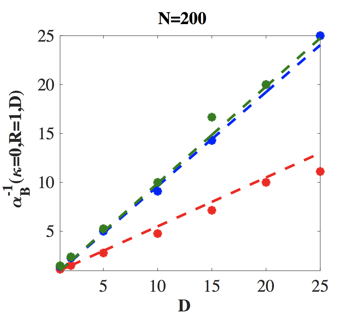
Figure 14: Capacity of high dimensional $L_{2}$ balls. $\alpha=P/N$ at capacity with $\kappa=0$ as a function of D. (red) $R=1$ (blue) $R=5$ (green) $R=10$. (markers) Simulation results. (dashed) full evaluation of $\alpha_{B}(\kappa=0,R,D)$. Note that for $R>5$, $\alpha_{B}^{-1}(\kappa=0,R\gg 1,D)\sim D$ .

Linear Classification of $L_{1}$ Balls

Sampling of $L_{1}$ Balls.

Because the sides of $L_{1}$ balls are straight lines, if all the vertices are on the same side of the plane, all the points in the interior of $L_{1}$ ball are on the same side of the plane as well. Therefore linear classifications of the entire $L_{1}$ball is equivalent to linear classification of all the vertices. In Fig. 3 (main text), we consider $D=2,$ thus, we simulated SVM solutions of the $4P$ points, $\mathbf{z}^{\mu}=\mathbf{x_{0}}^{\mu}\pm R\mathbf{u}_{1}^{\mu}\pm R\mathbf{u}_{2}^{\mu}$ where each set of $4$ points on the same manifold receive the same label. In the simulations shown in the figure, network size of $N=200$ was used and the simulation was repeated 100 times to get the convergence rate (of 0.5 for estimating capacity). The fractions of manifold geometry configurations were computed similarly to the previous cases. Here, however, there are $4$ configurations, corresponding to configurations with $0,1,2,$ or $4$ number of vertices on the margin plane.

The Maximum Margin Manifold Machines

Introduction

Handling object variability is a major challenge for machine learning systems. For example, in visual recognition tasks, changes in pose, lighting, identity or background can result in large variability in the appearance of objects ^{hinton1997modeling}. Techniques to deal with this variability has been the focus of much recent work, especially with convolutional neural networks consisting of many layers. The manifold hypothesis states that natural data variability can be modeled as lower-dimensional manifolds embedded in higher dimensional feature representations ^{bengio2013representation}. A deep neural network can then be understood as disentangling or flattening the data manifolds so that they can be more easily read out in the final layer ^{brahma2016deep}. Manifold representations of stimuli have also been utilized in neuroscience, where different brain areas are believed to untangle and reformat their representations ^{riesenhuber1999hierarchical, serre2005object, hung2005fast, dicarlo2007untangling, pagan2013signals}.

This chapter addresses the problem of efficiently utilizing manifold structures to learn classifiers. The manifold structures may be known from prior knowledge, or could be estimated from data using a variety of manifold learning algorithms ^{tenenbaum1998mapping, roweis2000nonlinear, tenenbaum2000global, belkin2003laplacian, belkin2006manifold, canas2012learning}. Based upon knowledge of these structures, some areas of prior research have focused on building invariant representations ^{anselmi2013unsupervised} or constructing invariant metrics ^{simard1994memory}. On the other hand, most approaches today rely upon data augmentation by explicitly generating “virtual” examples from these manifolds ^{niyogi1998incorporating, scholkopf1996incorporating}. Unfortunately, the number of samples needed to successfully learn the underlying manifolds may increase the original training set by more than a thousand-fold ^{krizhevsky2012imagenet}.

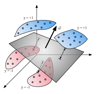
Figure 15: The maximum margin manifold binary classification problem. The optimal linear hyperplane is parameterized by the weight vector $\vec{w}$ which separates positively labeled manifolds from negatively labeled manifolds. Traditional data augmentation techniques would sample a large number of points from each manifold to train a conventional SVM.

We propose a new method, called the Maximum Margin Manifold Machine or $M^{4}$, that uses knowledge of the manifolds to efficiently learn a maximum margin classifier. Figure 15 illustrates the problem in its simplest form, binary classification of manifolds with a linear hyperplane. Given a number of manifolds embedded in a feature space, the $M^{4}$ algorithm learns a weight vector $\vec{w}$ that separates positively labeled manifolds from negatively labeled manifolds with the maximum margin. Although the manifolds consist of uncountable sets of points, the $M^{4}$ algorithm is able to find a good solution in a provably finite number of iterations and training examples.

Support vector machines (SVM) are widely used method to learn a maximum margin classifier based upon a set of training examples ^{vapnik1998statistical}. However, the standard SVM algorithm quickly becomes computationally intractable in time and memory as the number of training examples increases, rendering data augmentation methods impractical for SVMs. Methods to reduce the space complexity of SVM have been studied before, in the context of dealing with large-scale datasets. Chunking makes large problems solvable by breaking up the problem into subproblems ^{smola1998learning}, but the resultant kernel matrix may still be very large. One method that subsamples the training data include the reduced SVM (RSVM), which utilize a random rectangular subset of the kernel matrix ^lee2001rsvm. But this approach and other methods that attempt to reduce the number of training samples ^{wang2005training, smola1998learning} may result in suboptimal solutions that do not generalize well.

Our $M^{4}$ algorithm directly handles the uncountable set of points in the manifolds by solving a quadratic semi-infinite programming problem (QSIP). $M^{4}$ is based upon a cutting-plane method which iteratively refines a finite set of training examples to solve the underlying QSIP ^{fang2001solving, kortanek1993central, liu2004new}. The cutting-plane method was also previously shown to efficiently handle learning problems with a finite number of examples but an exponentially large number of constraints ^{joachims2006training}. We provide a novel analysis of the convergence of $M^{4}$ with both hard and soft margins. When the problem is realizable, the convergence bound explicitly depends upon the margin value whereas with a soft margin and slack variables, the bound depends linearly on the number of manifolds.

The chapter is organized as follows. We first consider the hard margin problem and analyze the simplest form of the $M^{4}$ algorithm. Next, we introduce slack variables in $M^{4}$, one for each manifold, and analyze its convergence with those additional auxiliary variables. We then demonstrate application of $M^{4}$ to both synthetic data where the manifold geometry is known as well as to actual object images undergoing a variety of warpings. We compare its performance, both in efficiency and generalization error, with conventional SVMs using data augmentation techniques. Finally, we discuss some natural extensions and potential future work on $M^{4}$ and its applications.

Maximum Margin Manifold Machines with Hard Margin

In this section, we first consider the problem of classifying a set of manifolds when they are linearly separable. This allows us to introduce the simplest version of the $M^{4}$ algorithm along with the appropriate definitions and QSIP formulation. We analyze the convergence of the simple algorithm and prove an upper bound on the number of errors the algorithm can make in this setting.

Hard Margin QSIP

Formally, we are given a set of $P$ manifolds $M_{p}\subset\mathbb{R}^{N}$, $p=1,\ldots,P$ with binary labels $y_{p}=\pm 1$ (all points in the same manifold share the same label). Each $M_{p}$ is defined by a parametrization $\vec{x}=M_{p}(\vec{s}$) where $\vec{s}\in S_{p}$, $S_{p}$ is a compact subset of $\mathbb{R}^{D}$, $M_{p}(\vec{s}):\mathbb{R}^{D}\rightarrow\mathbb{R}^{N}$ is a continuous function of $\vec{s}\in S_{p}$ so that the manifolds are bounded: $\forall\vec{s},\,\left\|M_{p}(\vec{s})\right\|<L$ by some $L$. We would like to solve the following semi-infinite quadratic programming problem for the weight vector $\vec{w}\in\mathbb{R}^{N}$ :

$$\begin{array}[]{c}SVM_{simple}:\underset{\vec{w}}{\text{argmin}}\frac{1}{2}\left\|\vec{w}\right\|^{2}\\ s.t.\;\forall p,\forall\vec{x}\in M_{p}:\;y_{p}\left\langle\vec{w},\vec{x}\right\rangle\geq 1\end{array}$$ (137)

This is the primal formulation of the problem, where maximizing the margin $\kappa=\frac{1}{||\vec{w}||}$ is equivalent to minimizing the squared norm $\frac{1}{2}||\vec{w}||^{2}.$ We denote the maximum margin attainable by $\kappa^{*}$, and the optimal solution as $\vec{w}^{*}$. For simplicity, we do not explicitly include the bias term here. A non-zero bias can be modeled by adding an additional feature of constant value as a component to all the $\vec{x}$. Note that the dual formulation of this QSIP is more complicated, involving optimization of non-negative measures over the manifolds. In order to solve the hard margin QSIP, we propose the following simple $M^{4}$ algorithm.

$M_{simple}^{4}$ Algorithm

The $M_{simple}^{4}$ algorithm is an iterative algorithm to find the optimal $\vec{w}$ in (137), based upon a cutting plane method for solving the QSIP. The general idea behind $M_{simple}^{4}$ is to start with a finite number of training examples, find the maximum margin solution for that training set, augment the training set by looking for a point on the manifolds that most violates the constraints, and iterating this process until a tolerance criterion is reached.

At each stage $k$ of the algorithm there is a finite set of training points and associated labels. The training set at the $k$-th iteration is denoted by the set: $T_{k}=\left\{\left(\vec{x}^{i}\in M_{p_{i}},y_{p_{i}}\right)\right\}$ with $i=1,\ldots,\left|T_{k}\right|$ examples. For the $i$-th pattern in $T_{k}$, $p_{i}$ is the index of the manifold, and $y_{p_{i}}$ is its associated label.

On this set of examples, we solve the following finite quadratic programming problem:

$$\begin{array}[]{c}SVM_{T_{k}}:\underset{\vec{w}}{\text{argmin}}\frac{1}{2}\left\|\vec{w}\right\|^{2}\\ s.t.\forall\vec{x}^{i}\in T_{k}:\;y_{p_{i}}\left\langle\vec{w},\vec{x}^{i}\right\rangle\geq 1\end{array}$$ (138)

to obtain the optimal weights $\vec{w}^{(k)}$ on the training set $T_{k}$. We then find a worst constraint-violating point $\vec{x}_{k+1}\in M_{p_{k+1}}$ from one of the manifolds such that

$$\left\{p_{k+1},\,\vec{x}_{k+1}\right\}:\underset{p,\,\vec{x}\in M_{p}}{\text{argmin}}y_{p}\left\langle\vec{w}^{(k)},\vec{x}\right\rangle<1-\text{$\delta$}$$ (139)

with a required tolerance $\delta>0.$ If there is no such point, the $M_{simple}^{4}$ algorithm terminates. If such a point exists, it is added to the training set, defining the new set $T_{k+1}=T_{k}\cup\left\{\left(\vec{x}_{k+1},y_{p_{k+1}}\right)\right\}$. The algorithm then proceeds at the next iteration to solve $SVM_{T_{k+1}}$to obtain $\vec{w}^{(k+1)}$. For $k=1$, the set $T_{1}$ is initialized with at least one point from each manifold. The pseudocode for $M_{simple}^{4}$ is shown in 2.

1. Input: $\delta$ (tolerance), $P$ manifolds and labels $\left\{M_{p},\,y_{p}=\pm 1\right\}$, $p=1,...,P$.

2. Initialize the iteration number $k=1$, and the set $T_{1}=\left\{\left(\vec{x}^{i}\in M_{p_{i}},\,y_{p_{i}}\right)\right\}$ with at least one sample from each manifold $M_{p}$.

3. Solve for $\vec{w}^{(k)}$ in $SVM_{T_{k}}$: $\min\frac{1}{2}\left\|\vec{w}\right\|^{2}$ such that $y^{p_{i}}\langle\vec{w,}\vec{x}^{i}\rangle\geq 1$ for all $\left(x^{i},y^{p_{i}}\right)\in T_{k}$.

4. Find a worst point $x^{k+1}\in M_{p_{k+1}}$ among the manifolds $\left\{p_{k+1}=1,...,P\right\}$ with a margin smaller than $1-\delta$:

   $$\vec{x}_{k+1}=\underset{\vec{x}\in M_{p_{k+1}},p_{k+1}=1,...P}{\text{argmin}}y_{p_{k+1}}\left\langle\vec{w}^{(k)},\vec{x}\right\rangle<1-\text{$\delta$}$$

5. If there is no such point, then stop. Else, augment the point set: $T_{k+1}=T_{k}\cup\left\{\left(\vec{x}_{k+1},y_{p_{k+1}}\right)\right\}$.

6. $k\leftarrow k+1$ and go to 3.

Algorithm 2 Pseudocode for the $M_{simple}^{4}$ algorithm.

In step 4 of the $M_{simple}^{4}$ algorithm, a point among the manifolds needs to be found with the worst margin constraint violation. This is particularly convenient if the manifolds are given by analytic parametric forms, where this point could be computed analytically as for the case of manifolds with $L_{2}$ balls or ellipses. However, for the algorithm to converge it is sufficient that a constraint violation point is found. Thus, local optimization procedures such as gradient descent may be used to search for such a point. However, the speed of convergence in the latter stages of $M_{simple}^{4}$ might be improved by a larger difference in the constraint violation of the point found in this step.

Convergence of $M_{simple}^{4}$

The $M_{simple}^{4}$ algorithm will converge asymptotically to an optimal solution when it exists. Here we show that the $\vec{w}^{(k)}$ asymptotically converges to an optimal $\vec{w}^{\star}$. Denote the change in the weight vector in the $k$-th iteration as $\Delta\vec{w}^{(k)}=\vec{w}^{(k+1)}-\vec{w}^{(k)}$. First we have the following lemma:

Lemma 1.

The change in the weights satisfies $\langle\Delta\vec{w}^{(k)},\vec{w}^{(k)}\rangle\geq 0$ .

Proof.

Define $\vec{w}(\lambda)=\vec{w}^{(k)}+\lambda\Delta\vec{w}^{(k)}$. Then for all $0\leq\lambda\leq 1$, $\vec{w}(\lambda)$ satisfies the constraints on the point set $T_{k}$: $y_{p_{i}}\left\langle\vec{w}(\lambda),\vec{x}_{i}\right\rangle\geq 1$ for all $\left(\vec{x}_{i},y_{p_{i}}\right)\in T_{k}$. However, if $\langle\Delta\vec{w}^{(k)},\vec{w}^{(k)}\rangle<0$, there exists a $0<\lambda^{\prime}<1$ such that $\left\|\vec{w}(\lambda^{\prime})\right\|^{2}<\left\|\vec{w}^{(k)}\right\|^{2}$, contradicting the fact that $\vec{w}^{(k)}$ is a solution to $SVM_{T_{k}}$. ∎

Next, we show that the norm $\left\|\vec{w}^{(k)}\right\|^{2}$ must monotonically increase by a finite amount at each iteration.

Theorem 2.

In the $k_{th}$ iteration of $M_{simple}^{4}$ algorithm, the increase in the norm of $\vec{w}^{(k)}$ is lower bounded by $\left\|\vec{w}^{(k+1)}\right\|^{2}\geq\left\|\vec{w}^{(k)}\right\|^{2}+\frac{\delta_{k}^{2}}{L^{2}}$, where $\delta_{k}=1-y_{p_{k+1}}\left\langle\vec{w}^{(k)},\vec{x}_{k+1}\right\rangle$ and $\left\|\vec{x}_{k+1}\right\|\leq L$ .

Proof.

First, note that $\delta_{k}>\delta\geq 0$ , otherwise the algorithm stops. We have: $\left\|\vec{w}^{(k+1)}\right\|^{2}=\left\|\vec{w}^{(k)}+\Delta\vec{w}^{(k)}\right\|^{2}$$=\left\|\vec{w}^{(k)}\right\|^{2}+\left\|\Delta\vec{w}^{(k)}\right\|^{2}+2\left\langle\vec{w}^{(k)},\Delta\vec{w}^{(k)}\right\rangle$ $\geq\left\|\vec{w}^{(k)}\right\|^{2}+\left\|\Delta\vec{w}^{(k)}\right\|^{2}$ due to Lemma 1. Now we consider the point added to set $T_{k+1}=T_{k}\cup\left(\vec{x}_{k+1},y_{p_{k+1}}\right)$. At this point, we know $y_{p_{k+1}}\left\langle\vec{w}^{(k+1)},\overrightarrow{x}_{k+1}\right\rangle\geq 1$, $y_{p_{k+1}}\left\langle w^{(k)},\overrightarrow{x}_{k+1}\right\rangle=1-\delta_{k}$, hence $y_{p_{k+1}}\left\langle\Delta\vec{w}^{(k)},\vec{x}_{k+1}\right\rangle\geq\delta_{k}$. Then, from the Cauchy-Schwartz inequality,

$$\left\|\Delta\vec{w}^{(k)}\right\|^{2}\geq\frac{\delta_{k}^{2}}{\left\|\vec{x}_{k+1}\right\|^{2}}>\frac{\delta_{k}^{2}}{L^{2}}>\frac{\delta^{2}}{L^{2}}$$ (140)

Since the optimal solution $\vec{w}^{\star}$ satisfies the constraints for $T_{k}$, we have $\left\|\vec{w}^{(k)}\right\|\leq\frac{1}{\kappa^{*}}$. We thus have a sequence of iterations whose norms monotonically increase and are upper bounded by $\frac{1}{\kappa^{\star}}$. Due to convexity, there is a single global optimum and the $M_{simple}^{4}$ algorithm is guaranteed to converge, asymptotically if the tolerance $\delta=0$, and in a finite number of steps if $\delta>0$ . ∎

As a corollary, we see that this procedure is guaranteed to find a realizable solution if it exists in a finite number of steps.

Corollary 3.

The $M_{simple}^{4}$ algorithm converges to a zero error classifier in less than $\frac{L^{2}}{\left(\kappa^{\star}\right)^{2}}$ iterations, where $\kappa^{\star}$ is the optimal margin and $L$ bounds the norm of the points on the manifolds.

Proof.

When there is an error, we have $\delta_{k}>1$, and $\left\|\vec{w}^{(k+1)}\right\|^{2}\geq\left\|\vec{w}^{(k)}\right\|^{2}+\frac{1}{L^{2}}$ (See (140)). This implies the total number of possible errors is upper bounded by $\frac{L^{2}}{\left(\kappa^{\star}\right)^{2}}$. ∎

With a finite tolerance $\delta>0$, we obtain a bound on the number of iterations required for convergence:

Corollary 4.

The $M_{simple}^{4}$ algorithm for a given tolerance $\delta>0$ will terminate after a finite number of iterations, with less than $\frac{L^{2}}{\left(\kappa^{\star}\delta\right)^{2}}$ iterations where $\kappa^{\star}$ is the optimal margin and $L$ bounds the norm of the points on the manifolds.

Proof.

Again, $\left\|\vec{w}^{k}\right\|^{2}\leq\left\|\vec{w}^{\star}\right\|^{2}=\frac{1}{\left(\kappa^{\star}\right)^{2}}$ and each iteration increases the squared norm by at least $\frac{\delta^{2}}{L^{2}}$. ∎

We can also bracket the error in the objective function after $M_{simple}^{4}$ terminates:

Corollary 5.

With tolerance $\delta>0$, after $M_{simple}^{4}$ terminates with solution $\vec{w}_{M^{4}}$, the optimal value $\left\|\vec{w}^{\star}\right\|$ of $SVM_{simple}$ is bracketed by:

$$\left\|\vec{w}_{M^{4}}\right\|^{2}\leq\left\|\vec{w}^{\star}\right\|^{2}\leq\frac{1}{\left(1-\delta\right)^{2}}\left\|\vec{w}_{M^{4}}\right\|^{2}.$$ (141)

Proof.

The lower bound on $\left\|\vec{w}^{\star}\right\|^{2}$ is as before. Since $M_{simple}^{4}$ has terminated, setting $\vec{w}^{\prime}=\frac{1}{(1-\delta)}\vec{w}_{M^{4}}$ would make $\vec{w}^{\prime}$ feasible for $SVM_{simple}$, resulting in the upper bound on $\left\|\vec{w}^{\star}\right\|^{2}$. ∎

$M^{4}$ with Slack Variables

In many classification problems, the manifolds may not be linearly separable due to their dimensionality, size, and/or correlations. In these situations, $M_{simple}^{4}$ will not even be able to find a feasible solution. To handle these problems, the classic approach is to introduce slack variables. Naively, we could introduce a slack variable for every point on the manifolds as below:

$$\begin{array}[]{c}SVM_{naive}^{slack}:\underset{\vec{w},\xi_{p}(\vec{x})}{\text{argmin}}\frac{1}{2}\left\|\vec{w}\right\|^{2}+C\sum_{p=1}^{P}\int_{\vec{x}\in M_{p}}\xi_{p}(\vec{x})\\ s.t.\;\forall p,\forall\vec{x}\in M_{p}:\;y_{p}\left\langle\vec{w},\vec{x}\right\rangle+\xi_{p}(\vec{x})\geq 1,\\ \xi_{p}(\vec{x})\geq 0\end{array}$$

The parameter $C$ represents the tradeoff between fitting the manifolds to obey the margin constraints while allowing some set of points to be misclassified. This approach cannot be used when training data consists of entire manifolds as in general, it would require replacing the sum over a finite number of training points in the cost function, to an integral with an appropriate measure over the manifolds. Thus, we formulate an alternative version of the QSIP with slack variables below.

QSIP with Manifold Slacks

In this work, we propose using only one slack variable per manifold for classification problems with non-separable manifolds. This formulation demands that all the points on each manifold $\vec{x}\in M_{p}$ obey an inequality constraint with one manifold slack variable, $y_{p}\left\langle\vec{w},\vec{x}\right\rangle+\xi_{p}\geq 1$. As we see below, solving for this constraint is tractable and the algorithm has good convergence guarantees.

However, this single slack requirement for each manifold by itself may not be sufficient for good generalization performance. Indeed, our empirical studies show that generalization performance can be improved if we additionally demand that some representative points $\vec{x}_{p}\in M_{p}$ on each manifold also obey the margin constraint: $y_{p}\left\langle\vec{w},\vec{x}_{p}\right\rangle\geq 1$. In this work, we implement this intuition by specifying appropriate center points $\vec{x}_{p}^{c}$ for each manifold $M_{p}$. This center point could be the center of mass of the manifold, a representative point, or an exemplar used to generate the manifolds ^{krizhevsky2012imagenet}. For simplicity, we demand that these points strictly obey the margin inequalities corresponding to their manifold label, but we could have alternatively introduced additional slack variables for these constraints. Formally, the QSIP optimization problem is summarized below, where the objective function is minimized over the weight vector $\vec{w}\in\mathbb{R}^{N}$ and slack variables $\vec{\xi}\in\mathbb{R}^{P}$:

$$\begin{array}[]{c}SVM_{manifold}^{slack}:\,\underset{\vec{w},\vec{\xi}}{\text{argmin}}F(\vec{w},\vec{\xi})=\frac{1}{2}\left\|\vec{w}\right\|^{2}+C\sum_{p=1}^{P}\xi_{p}\\ s.t.\;\forall p,\forall\vec{x}\in M_{p}:\;y_{p}\left\langle\vec{w},\vec{x}\right\rangle+\xi_{p}\geq 1\ \text{(manifolds)}\\ \forall p:\ y_{p}\left\langle\vec{w},\vec{x}_{p}^{c}\right\rangle\geq 1\ \text{(centers)}\\ \forall p:\;\xi_{p}\geq 0\end{array}$$

$M_{slack}^{4}$ Algorithm

With these definitions, we introduce our $M_{slack}^{4}$ algorithm with slack variables below.

1. Input: $\delta$ (tolerance), $P$ manifolds and labels $\left\{M_{p},y_{p}=\pm 1\right\}$, and centers $\vec{x}_{p}^{c}$

2. Initialize the iteration number $k=1$, and the set $T_{1}=\left\{\left(\vec{x}^{i}\in M_{p_{i}},\,y_{p_{i}}\right)\right\}$ with at least one sample from each manifold $M_{p}$.

3. Solve for $\vec{w}^{(k)}$,$\vec{\xi}^{(k)}$: $\min\frac{1}{2}\left\|\vec{w}\right\|^{2}+C\sum_{p=1}^{P}\xi_{p}$ such that $y_{p_{\mu}}\langle\vec{w,}\vec{x}^{\mu}\rangle+\xi_{p_{\mu}}\geq 1$ for all $\left(\vec{x}^{\mu},y_{p_{\mu}}\right)\in T_{k}$ and $y_{p}\langle\vec{w,}\vec{x}_{p}^{c}\rangle\geq 1$ for all $p$.

4. Find a point $\vec{x}^{k+1}\in M_{p_{k+1}}$ among the manifolds $\left\{p=1,...,P\right\}$ with slack violation larger than the tolerance $\delta$:

   $$y_{p_{k+1}}\left\langle\vec{w}^{(k)},\vec{x}_{k+1}\right\rangle+\xi_{p_{k+1}}<1-\text{$\delta$}$$

5. If there is no such point, then stop. Else, augment the point set: $T_{k+1}=T_{k}\cup\left\{\left(\vec{x}_{k+1},y_{p_{k+1}}\right)\right\}$.

6. $k\leftarrow k+1$ and go to 3.

Algorithm 3 Pseudocode for the $M_{slack}^{4}$ algorithm.

The proposed $M_{slack}^{4}$ algorithm modifies the cutting plane approach to solve a semi-infinite, semi-definite quadratic program. Each iteration involves a finite set: $T_{k}=\left\{\left(\vec{x}^{i}\in M_{p_{i}},y_{p_{i}}\right)\right\}$ with $i=1,\ldots,\left|T_{k}\right|$ examples that is used to define the following soft margin SVM:

$$\begin{array}[]{c}SVM_{T_{k}}^{slack}:\underset{\vec{w},\vec{\xi}}{\text{argmin}}\frac{1}{2}\left\|\vec{w}\right\|^{2}+C\sum_{p=1}^{P}\xi_{p}\\ s.t.\;\forall\left(\vec{x}^{i},y_{p_{i}}\right)\in T_{k}:\;y_{p_{i}}\left\langle\vec{w},\vec{x}^{i}\right\rangle+\xi_{p_{i}}\geq 1\\ \forall p:\ y_{p}\left\langle\vec{w},\vec{x}_{p}^{c}\right\rangle\geq 1\;(centers)\\ \forall p:\;\xi_{p}\geq 0\end{array}$$

to obtain the weights $\vec{w}^{(k)}$ and slacks $\vec{\xi}^{(k)}$ at each iteration. We then find a point $\vec{x}_{k+1}\in M_{p_{k+1}}$ from one of the manifolds so that:

$$y_{p_{k+1}}\left\langle\vec{w}^{(k)},\vec{x}_{k+1}\right\rangle+\xi_{p_{k+1}}^{(k)}=1-\delta_{k}$$ (142)

where $\delta_{k}>\delta$. If there is no such a point, the $M_{slack}^{4}$ algorithm terminates. Otherwise, the point $\vec{x}_{k+1}$ is added as a training example to the set $T_{k+1}=T_{k}\cup\left\{\left(\vec{x}_{k+1},y_{p_{k+1}}\right)\right\}$ and the algorithm proceeds to solve $SVM_{T_{k+1}}^{slack}$ to obtain $\vec{w}^{(k+1)}$ and $\vec{\xi}^{(k+1)}$. Note that $M_{slack}^{4}$ embodies the fact that for the algorithm to converge, it is not necessary to find the point with the worst constraint violation at each iteration.

Convergence of $M_{slack}^{4}$

Here we show that the objective function $F\left(\vec{w},\vec{\xi}\right)=\frac{1}{2}\left\|\vec{w}\right\|^{2}+C\sum_{p=1}^{P}\xi_{p}$ is guaranteed to increase by a finite amount with each iteration. This result is similar to ^{tsochantaridis2005large}, but here we demonstrate a proof in the primal domain over an infinite number of examples. We first have the following lemmas,

Lemma 6.

The change in the weights and slacks satisfy:

$$\left\langle\Delta\vec{w}^{(k)},\vec{w}^{(k)}\right\rangle+C\sum_{p}\Delta\vec{\xi}_{p}^{(k)}\geq 0$$ (143)

where $\Delta\vec{w}^{(k)}=\vec{w}^{(k+1)}-\vec{w}^{(k)}$ and $\Delta\vec{\xi}^{(k)}=\vec{\xi}^{(k+1)}-\vec{\xi}^{(k)}$.

Proof.

Define $\vec{w}(\lambda)=\vec{w}^{(k)}+\lambda\Delta\vec{w}^{(k)}$ and $\vec{\xi}(\lambda)=\vec{\xi}^{(k)}+\lambda\Delta\vec{\xi}^{(k)}$. Then for all $0\leq\lambda\leq 1$, $\vec{w}(\lambda)$ and $\vec{\xi}(\lambda)$ satisfy the constraints for $SVM_{T_{k}}^{slack}$. The resulting change in the objective function is given by:

$$F\left(\vec{w}(\lambda),\vec{\xi}(\lambda)\right)-F\left(\vec{w}^{(k)},\vec{\xi}^{(k)}\right)=\\ \lambda\left[\left\langle\Delta\vec{w}^{(k)},\vec{w}^{(k)}\right\rangle+C\sum_{p}\Delta\xi_{p}^{(k)}\right]+\frac{1}{2}\lambda^{2}\left\|\Delta\vec{w}^{(k)}\right\|^{2}$$ (144)

If (143) is not satisfied, then there is some $0<\lambda^{\prime}<1$ such that $F\left(\vec{w}(\lambda^{\prime}),\vec{\xi}(\lambda^{\prime})\right)<F\left(\vec{w}^{(k)},\vec{\xi}^{(k)}\right)$, which contradicts the fact that $\vec{w}^{(k)}$ and $\vec{\xi}^{(k)}$ are a solution to $SVM_{T_{k}}$. ∎

Lemma 7.

In each iteration of $M_{slack}^{4}$ algorithm, the added point $\left(\vec{x}_{k+1},y_{p_{k+1}}\right)$ must be a support vector for the new weights and slacks, s.t.

$$y_{p_{k+1}}\left\langle\vec{w}^{(k+1)},\vec{x}_{k+1}\right\rangle+\xi_{p_{k+1}}^{(k+1)}=1$$ (145)

and

$$y_{p_{k+1}}\left\langle\Delta\vec{w}^{(k)},\vec{x}_{k+1}\right\rangle+\Delta\xi_{p_{k+1}}^{(k)}=\delta_{k}$$ (146)

Proof.

Suppose $y_{p_{k+1}}\left\langle\vec{w}^{(k+1)},\vec{x}_{k+1}\right\rangle+\xi_{p_{k+1}}^{(k+1)}=1+\epsilon$ for some $\epsilon>0$. Then we can choose $\lambda^{\prime}=\frac{\delta_{k}}{\delta_{k}+\epsilon}<1$ so that $\vec{w}(\lambda^{\prime})=\vec{w}^{(k)}+\lambda^{\prime}\Delta\vec{w}^{(k)}$ and $\vec{\xi}(\lambda^{\prime})=\vec{\xi}^{(k)}+\lambda^{\prime}\Delta\vec{\xi}^{(k)}$ satisfy the constraints for $SVM_{T_{k+1}}^{slack}$. But, from Lemma 6, we have $F\left(\vec{w}(\lambda^{\prime}),\vec{\xi}(\lambda^{\prime})\right)<F\left(\vec{w}^{(k+1)},\vec{\xi}^{(k+1)}\right)$ which contradicts the fact that $\vec{w}^{(k+1)}$ and $\text{$\vec{\xi}$}^{(k+1)}$ are a solution to $SVM_{T_{k+1}}$. Thus, $\epsilon=0$ and the point $\left(\vec{x}_{k+1},y_{p_{k+1}}\right)$ must be a support vector for $SVM_{T_{k+1}}.$ (146) results from subtracting (142) from (145). ∎

We also derive a bound on the following quadratic function over nonnegative values:

Lemma 8.

Given $K>0$,$\delta>0$, then $\forall x\geq 0$

$$\frac{1}{2}(x-\delta)^{2}+Kx\geq\min\left(\frac{1}{2}\delta^{2},\frac{1}{2}K\delta\right)$$ (147)

Proof.

The minimum value occurs when $x^{\star}=\left[\delta-K\right]_{+}$. When $K\geq\delta$, then $x^{\star}=0$ and the minimum is $\frac{1}{2}\delta^{2}$. When $K<\delta$, the minimum occurs at $K\left(\delta-\frac{1}{2}K\right)\geq\frac{1}{2}K\delta$. Thus, the lower bound is the smaller of these two values. ∎

Theorem 9.

In each iteration $k$ of $M_{slack}^{4}$ algorithm, the increase in the objective function for $SVM_{manifold}^{slack}$ is lower bounded by

$$\Delta F^{(k)}\geq\min\left(\frac{1}{8}\frac{\delta_{k}^{2}}{L^{2}},\,\frac{1}{2}C\delta_{k}\right)$$ (148)

where $\Delta F^{(k)}=F\left(\vec{w}^{(k+1)},\vec{\xi}^{(k+1)}\right)-F\left(\vec{w}^{(k)},\vec{\xi}^{(k)}\right)$.

Proof.

(Sketch) First, if $\Delta\vec{w}^{(k)}\neq 0$, Lemma 6 completes the proof. If $\Delta\vec{w}^{(k)}=0$, then $\Delta\xi_{p_{k}}^{(k)}=\delta_{k}$ from Lemma 7 and $\Delta\xi_{p\neq p_{k}}^{(k)}=0$ since $\vec{\xi}^{(k)}$ is the solution for $SVM_{T_{k}}$. So for $\Delta\vec{w}^{(k)}=0$, $\Delta F^{(k)}=C\delta_{k}$.

The added point $\vec{x}_{k+1}$ is from a particular manifold $M_{p_{k+1}}$. If $\Delta\xi_{p_{k+1}}^{(k)}\leq 0$, we have $y_{p_{k+1}}\left\langle\Delta\vec{w}^{(k)},\vec{x}_{k+1}\right\rangle\geq\delta_{k}$ ($\because$ Lemma 7). Then, $\left\|\Delta\vec{w}^{(k)}\right\|^{2}\geq\frac{\delta_{k}^{2}}{L^{2}}$ , yielding $\Delta F^{(k)}\geq\frac{1}{2}\frac{\delta_{k}^{2}}{L^{2}}$.

We next analyze $\Delta\xi_{p_{k+1}}^{(k)}>0$ and consider the finite set of points $\left(\vec{x}^{\nu},\,p_{k+1}\right)\in T_{k}$, coming from the $p_{k+1}$ manifold. Each of these points obeys the constraints:

$$y_{p_{k+1}}\left\langle\vec{w}^{(k)},\vec{x}^{\nu}\right\rangle+\xi_{p_{k+1}}^{(k)} =1+\epsilon_{\nu}^{(k)}$$ (149)

$$y_{p_{k+1}}\left\langle\vec{w}^{(k+1)},\vec{x}^{\nu}\right\rangle+\xi_{p_{k+1}}^{(k+1)} =1+\epsilon_{\nu}^{(k+1)}$$ (150)

$$\epsilon_{\nu}^{(k)},\,\epsilon_{\nu}^{(k+1)} \geq 0$$ (151)

We consider the minimum value of the thresholds: $\eta=\min_{\nu}\epsilon_{\nu}^{(k)}$.

If $\eta>0$, none of the $\vec{x}^{\nu}$ points are support vectors for $SVM_{T_{k}}^{slack}$. In this case, we define a linear set of slack variables: $\xi_{p}(\lambda)=\xi_{p_{k}}^{(k)}$ for $p=p_{k}$, and $\xi_{p}(\lambda)=\xi_{p}^{(k)}+\lambda\Delta\xi_{p}^{(k)}$ for $p\neq p_{k}$, and $\vec{w}(\lambda)=\vec{w}^{(k)}+\lambda\Delta\vec{w}^{(k)}$, which satisfy the constraints for $SVM_{T_{k}}$. Then, this implies

$$\left\langle\Delta\vec{w}^{(k)},\vec{w}^{(k)}\right\rangle+C\sum_{p\neq p_{k}}\Delta\vec{\xi}_{p}^{(k)}\geq 0$$ (152)

which implies $\Delta F^{(k)}\geq\min\left(\frac{1}{2L^{2}}\delta_{k}^{2},\,\frac{1}{2}C\delta_{k}\right)$.

If $\eta=0$, at least one support vector lies in $M_{p_{k+1}}$. Consider $\varepsilon=\min_{\epsilon_{\nu}^{(k)}=0}\epsilon_{\nu}^{(k+1)}\geq 0$.

We then define $\xi_{p}(\lambda)=\xi_{p_{k}}^{(k)}+\lambda\left(\Delta\xi_{p}^{(k)}-\varepsilon\right)$ for $p=p_{k}$, and $\xi_{p}(\lambda)=\xi_{p}^{(k)}+\lambda\Delta\xi_{p}^{(k)}$ for $p\neq p_{k}$, and $\vec{w}(\lambda)=\vec{w}^{(k)}+\lambda\Delta\vec{w}^{(k)}$. Then, there exists $0\leq\lambda\leq\lambda_{min}$ for which $\vec{\xi}(\lambda)$ and $\vec{w}(\lambda)$ satisfy the constraints for $SVM_{T_{k}}$, so that

$$\left\langle\Delta\vec{w}^{(k)},\vec{w}^{(k)}\right\rangle+C\sum_{p}\Delta\vec{\xi}_{p}^{(k)}\geq C\varepsilon$$ (153)

We also have a support vector $\left(\vec{x}^{\nu},\,p_{k+1}\right)\in T_{k}$, with $y_{p_{k}}\left\langle\Delta\vec{w}^{(k)},\vec{x}^{\nu}\right\rangle+\Delta\xi_{p_{k}}^{(k)}=\varepsilon$, then $\left\|\Delta\vec{w}^{(k)}\right\|^{2}\geq\frac{1}{4L^{2}}\left(\delta_{k}-\varepsilon\right)^{2}$ by using Lemma 7.

Then, by using Lemma (8) on $\varepsilon$, we get

$$\Delta F^{(k)}\geq\min\left(\frac{1}{8L^{2}}\delta_{k}^{2},\,\frac{1}{2}C\delta_{k}\right)$$ (154)

Thus, we obtain the final bound combining results from two cases of $\eta$. ∎

Since the $M_{slack}^{4}$ algorithm is guaranteed to increase the objective by a finite amount, it will terminate in a finite number of iterations if we require $\delta_{k}>\delta$ for some positive $\delta>0$.

Corollary 10.

The $M_{slack}^{4}$ algorithm for a given $\delta>0$ will terminate after at most $P\cdot\max\left(\frac{8CL^{2}}{\delta^{2}},\,\frac{2}{\delta}\right)$ iterations where $P$ is the number of manifolds, L bounds the norm of the points on the manifolds.

Proof.

$\vec{w}=0$ and $\xi_{p}=1$ is a feasible solution for $SVM_{manifold}^{slack}$. Therefore, the optimal objective function is upper-bounded by $F\left(\vec{w}=0,\vec{\xi}=1\right)=PC$. The upper bound on the number of iterations is then provided by Theorem (9). ∎

We can also bound the error in the objective function after $M_{slack}^{4}$ terminates:

Corollary 11.

With $\delta>0$, after $M_{slack}^{4}$ terminates with solution $\vec{w}_{M^{4}}$, slack $\vec{\xi}_{M^{4}}$ and value $F_{M^{4}}=F\left(\vec{w}_{M^{4}},\vec{\xi}_{M^{4}}\right)$, then the optimal value $F^{\star}$ of $SVM_{manifold}^{slack}$ is bracketed by:

$$F_{M^{4}}\leq F^{\star}\leq F_{M^{4}}+PC\delta.$$ (155)

Proof.

The lower bound on $F^{\star}$ is apparent since $SVM_{manifold}^{slack}$ includes $SVM_{T_{k}}^{slack}$ constraints for all $k$. Setting the slacks $\xi_{p}=\xi_{M^{4},p}+\delta$ will make the solution feasible for $SVM_{manifold}^{slack}$ resulting in the upper bound. ∎

Experiments

Synthetic Manifolds

Random $L_{2}$ balls

As an illustration of our method, we have generated manifolds consisting of random $D$-dimensional Euclidean balls with a given radius. Each manifold $M_{p}$ is described by a center vector $\vec{x}_{p}^{c}\in\mathbb{R}^{N}$ and $D$ basis vectors $\left\{\vec{u}_{i}^{p}\in\mathbb{R}^{N},\>i=1,...,D\right\}$. The points on the manifold can be parameterized as $M_{p}=\left\{\vec{x}\left|\vec{x}=\vec{x}_{p}^{c}+R\sum_{i=1}^{D}s_{i}\vec{u}_{i}^{p}\right.\right\}$ where $R$ is the radius of the ball and $\vec{s}\in\mathbb{R}^{D}$ are normalized so that $\sum_{i=1}^{D}s_{i}^{2}=1$.

Simulations

We compare the performance of $M^{4}$ to the conventional point SVM with samples uniformly drawn from the $L_{2}$ ball manifolds. Performance is measured by generalization error as a function of the number of samples used by the algorithm.

For these manifolds, the worst constraint-violating point can easily be computed by taking the derivative of the constraint $y^{p}\left[\vec{w}\cdot\left(\vec{x}_{0}^{p}+R\sum_{i=1}^{D}s_{i}\vec{u}_{i}^{p}\right)\right]+\xi_{p}\geq 1$ with respect to $\vec{s}$ for all $p$. This results in the analytic solution $s_{i}^{p,worst}=-\frac{y^{p}\vec{w}\cdot\vec{u_{i}^{p}}}{\sqrt{\sum_{i=1}^{D}\left(\vec{w}\cdot\vec{u_{i}^{p}}\right)^{2}}}$ . For problems with non-separable manifolds in $M_{slack}^{4}$, we used an additional single margin constraint per manifold given by the center $\vec{x}_{p}^{c}$.

We used the following parameters in the simulations shown below: embedding dimension $N=500$, manifold dimension $D=10$, radius $R=20$. With these parameters, the critical manifold capacity for linear classification is estimated to be $P_{critical}=48.3$ ^{chung2016linear}, hence we consider $P=46$ to test $M_{simple}^{4}$ and $P=50$ for the $M_{slack}^{4}$ simulations.

The results are presented in figure 16 for the separable case and non-separable case.

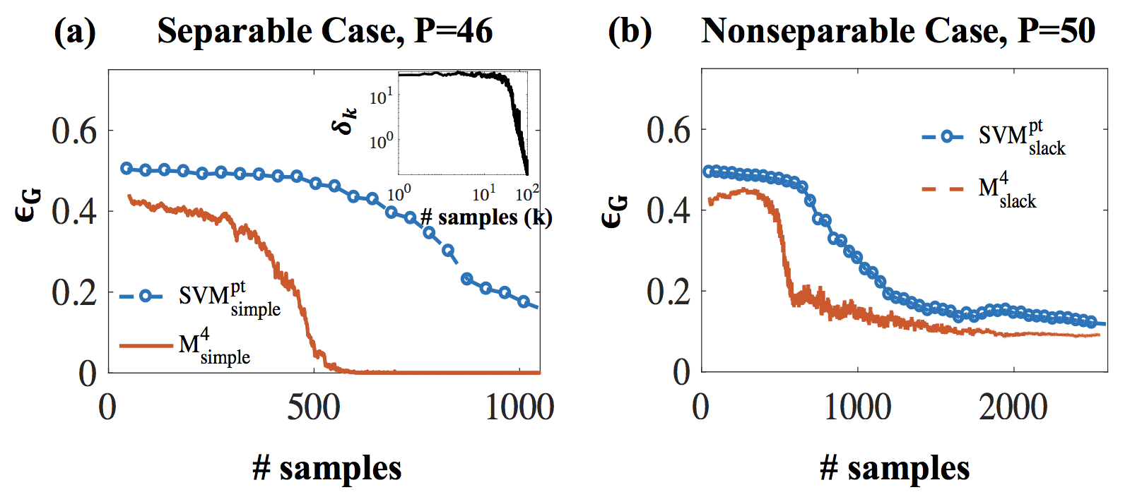
Figure 16: Generalization error of the $M^{4}$ solution for $L_{2}$ ball manifolds, shown as a function of the total number of training samples per manifold (red solid) compared with that of conventional point SVM (blue dashed). $N=500$, $D=10$, $R=20$, and (a) $P=46$ is used for $M_{simple}^{4}$and (b) $P=48$ for $M_{slack}^{4}$ with $C=100$. (a)-(Inset) $\delta_{k}$ is shown for the $k_{th}$ added point in $M_{simple}^{4}$. The critical capacity with these parameters is $P_{c}\approx 48$.

ImageNet Dataset

Image-based Object Manifolds

We also apply the $M^{4}$ algorithm to a more realistic class of object manifolds. Here each object manifold is defined by the infinite set of images created by applying 2-D affine transformations on a single template image. In order to create object manifolds, $P$ template images were sampled from the ImageNet 2012 data set for which exact object bounding boxes are available ^{deng2009imagenet}, and each image was cropped and scaled such that the object occupies the middle $48\times 48$ pixels of the template image.

Each sample from the object manifold is a $64\times 64$ gray-scale image created by applying a 2-D affine transformation on the template image. Those transformations are defined as a composition of seven basic transformations: horizontal or vertical translation, horizontal or vertical scaling, horizontal or vertical shear, and rotation. The range of each basic transformations was chosen so that the largest pixel displacement was equivalent to 8 pixels. The composition of these seven basic transformations thus defines a 7-D highly non-linear object manifold for each object.

Simulations

We compared the performance of $M^{4}$ to point SVM in classification of samples from the object manifolds. Performance is measured as above by generalization error as a function of the number of samples each algorithm uses. We used object manifolds with up to $M=10000$ samples drawn from each manifold, using $80\%$ of the samples as training set and $20\%$ as a testing set. Rather than performing classification directly on image pixels the samples were projected to the space defined by their $N=500$ largest principal components. For this data set the classification problem is separable for $P=4$ and non-separable for $P=6$.

Point SVM (defined as $SVM_{naive}^{slack}$ above) was trained with varying numbers of training set samples, with $C$ obtained through cross validation. The training was repeated $11$ times with different samples to estimate the variability of the generalization error. $M^{4}$ was trained with a constraint per manifold given by the center of mass at the training set

and $C$ obtained through cross-validation. At each iteration of the algorithm, the worst-violating constraint point was found using local search. Initialized with a random sample from each manifold, it was compared to a set of $K$ neighboring samples in the space of potential transformation ($K=5$ was used throughout). This process is iterated until a set of local minima were found, and these points were candidates to be added to the active set of the $M^{4}$ algorithm.

Figure 17-b compares the generalization error for a separable classification problem (at $P=4$) while Figure 17-c compare those for a non-separable classification problem (at $P=6$). Those representative results illustrate that in both cases $M^{4}$ achieve a very low generalization error (compared to point SVM) already at very small number of samples.

Figure 17: Image-based object manifolds. (a) Basic affine transformation: a template image (middle) surrounded with changes along 4 axes defined by basic affine transformation. A $48\times 48$ square marking the object bounding box was added to the template image for illustration purposes. (b-c) Generalization error of the $M^{4}$ solution for 7-D image-based object manifolds, shown as a function of the number of training samples per manifold (solid line) compared with that of conventional point SVM (blue squares). At $N=300$ the problem is separable for $P=4$ (b) and non-separable for $P=6$ (c).

Discussion

We described and analyzed a novel algorithm for finding the maximum margin solution for classifying manifolds. The algorithm, called $M^{4}$, is based upon a cutting-plane method and iterates between adding the worst violating point to a finite training set, and updating a maximum margin solution. There are two versions of the algorithm, one without slack variable appropriate for separable manifolds, and a slack version for non-separable manifolds. We proved the convergence of $M^{4}$, and provided bounds on the number of iterations required and the deviation from the optimal objective function. On experiments with both synthetic manifolds and with actual image manifolds, our empirical results demonstrate the efficiency of $M^{4}$ and the superior performance in terms of generalization error, compared to conventional SVM’s, using data augmentation techniques with many virtual examples. Ongoing work includes theoretical research to understand how $M^{4}$ explicitly scales with the number of manifolds and the embedding dimensionality.

There is natural extension of $M^{4}$ to nonlinear classifiers via the kernel trick, as all our operations involve dot products between the weight vector $\vec{w}$ and manifold points $M_{p}(\vec{s})$. At each iteration, the algorithm would solve the dual version of the $SVM_{T_{k}}$ problem which is readily kernelized. In addition, the $M^{4}$ algorithm relies upon finding a point on a manifold with sufficiently strong violation of the constraints. Since a local minimization of the constraint violation at each stage is sufficient in the relaxed version of the algorithm, we expect that this step of $M^{4}$ will be practical for simpler kernel functions. However, we note that with infinite-dimensional kernels such as RBF’s, the full manifold optimization problem becomes a fully infinite quadratic programming problem, no longer a QSIP which requires further theoretical work to establish the existence and properties of optimal solutions.

Beyond binary classification, variations of $M^{4}$ can also be used to solve other machine learning problems including multi-class classification, ranking, one-class learning, etc. In this work, we have shown how $M^{4}$ can be used to classify image manifolds at pixel input representations. We can also use this algorithm to evaluate the computational benefits of manifold representations at successive layers of deep networks in both machine learning and in brain sensory hierarchies. We also anticipate using $M^{4}$ to build novel hierarchical architectures that can incrementally reformat the manifold representations through the layers for better overall performance in machine learning tasks.

We anticipate this work will make an important contribution to the understanding of how neural architectures can learn to process high dimensional real-world signal ensembles and cope with large variability due to continuous modulation of the underlying physical parameters.

Linear Classification of General Manifolds

Introduction

In chapter Linear Classification of Spherical Manifolds, we applied methods from statistical mechanics of spin glasses to solve the problem of linear, max margin, classification of manifolds with simple geometries such as lines, as well as $L_{2}$and $L_{p}$ balls embedded in embedded in a linear subspace with dimensions $D$, where $D$ is much smaller than the ambient dimension $N$. In chapter The Maximum Margin Manifold Machines, we presented a new efficient algorithm for finding max margin linear classifier of manifolds.

In this chapter, we return to the theory and consider the problem of linear classification of general manifolds, again with embedding dimension much smaller than $N$. To set the stage of more complex geometries, we begin by considering the classification of $D$-dimensional $L_{2}$ ellipsoids. The results from the analysis of ellipsoids are readily extended to the case general smooth convex manifolds. We then move to consider classification of non-smooth low dimensional manifolds, which exhibit a more complex solution structure. characterized by variety of ’support’ structures. Nevertheless, we derive a set of mean field equations that apply to general low dimensional smooth as well as non-smooth manifolds, including also manifolds consisting of finite number of points (point clouds). We identify key geometric descriptors of the manifolds: the effective manifold dimension $D_{M}$ and the effective manifold radius $R_{M}$ , two geometric ’order parameters’ which determine the capacity of linear classification of general manifolds (when their dimensionality is high), and provide an iterative algorithm that can efficiently solve for $D_{M}$ and $R_{M}$ , as well as general manifold capacity $\alpha_{M}$ . Finally, we emphasize that although the data manifolds may not be convex, any hyperplane that separates them must also separate their convex hull. Hence, all geometric properties discussed in this chapter refer to convex manifolds.

Note that in general, the capacity of manifolds embedded in $D$ dimension can be upper and lower bounded by

$$\frac{2}{1+2D}<\alpha_{c}<2$$ (156)

This is because in the limit where extents of a manifold in all $D$ embedding dimensions go to zero, a manifold becomes a point, whose perceptron capacity is $\alpha_{0}=2$ ^{gardner1988space}. In the limit where extents of a manifold in all $D$ embedding dimensions go to infinity, then the linear classifier $\mathbf{w}$ has be in the subspace orthogonal to all $D$ directions of the $P$ manifolds ^{chung2016linear}. Since $P$ of the $D$-dimensional manifolds occupy $PD$ dimension, the classification becomes point classification in $N-PD$ dimension, resulting in the maximum number of manifolds linear separable $P=2(N-PD)$, resulting in the capacity $P/N=\frac{2}{1+2D}$. These asymptotic bounds of a manifold capacity apply for arbitrary manifold shapes. Now let us focus on simplest extension of classification of $L_{2}$ balls, classification of $D$ -dimensional ellipsoids.

$L_{2}$ Ellipsoids

Model

Consider the problem of linearly classifying $D$-dimensional ellipsoids (Figure. 18) in $N$-dimensional ambient space, where each point within the $\mu$th ellipsoid is expressed as

$$\left\{\mathbf{x}_{0}^{\mu}+\sum_{i=1}^{D}s_{i}\mathbf{u}_{i}^{\mu},y^{\mu}=\pm 1\right\}$$ (157)

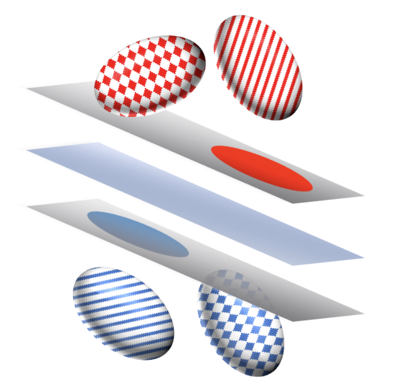
Figure 18: Linear Classification of Ellipsoids (Illustration). In $N$-dimensional ambient space, the solution hyperplane (blue plane) has to separate between red $D$-dimensional ellipsoids and blue ellipsoids with margin $\kappa$. Margin $\kappa$ is the distance between the closest point on the ellipsoids and the solution hyperplane. We refer to all points of such distance to the solution hyperplane as “margin planes” (grey planes). Different patterns are used to denote different support configuration of manifolds. Solid pattern: ellipsoids embedded in the margin plane, diamond pattern: ellipsoids touching the margin plane with one point, striped pattern: interior ellipsoids (ellipsoids that are in the interior space shattered by margin planes).

For each $\mu$, $\mathbf{x}_{0}^{\mu}\in\mathbb{R}^{N}$ is N-dim vector representing the center of the ellipsoid, the set of D N-dim vectors, $\mathbf{u}_{i}^{\mu}\in\mathbb{R}^{N}$, for $i=1,...,D$ , are the ellipsoid’s basis vectors. The vectors $\vec{s}\in\mathbb{R}^{D}$ parametrize the points on the manifolds and obey the constraint

$$f(\vec{s})\leq 0$$ (158)

where,

$$f(\vec{s}) =\sum_{i=1}^{D}s_{i}^{2}R_{i}^{-2}-1$$ (159)

$R_{i}$ represent the ellipsoid’s radii in the $i$ th direction, relative to the center norm. In order to evaluate the ability of the perceptron to classify the ellipsoids, we need to specify their statistical properties. Here we assume that each component of $\mathbf{x}_{0}^{\mu}$, $\mathbf{u}_{i}^{\mu}$ are independent Gaussian random variables with unit variance. With these assumptions, and assuming large $N$, the norm of the centers is (approximately) $\sqrt{N}$ and the $\mathbf{u}_{i}$’s are (approximately) orthogonal vectors with norms $\sqrt{N}$ .

We assume the ellipsoids are assigned binary labels (which are therefore the same for all points on the ellipsoid) denoted as $y^{\mu}=\pm 1$ . We search of a set of weight vectors $\mathbf{w}\in\mathbb{R}^{N}$ that obey the following inequalities,

$$y^{\mu}\mathbf{w}^{T}\left(\mathbf{x_{\mathbf{0}}}^{\mu}+\sum_{i=1}^{D}s_{i}\mathbf{u}_{i}^{\mu}\right)\geq\kappa\left\|\mathbf{w}\right\|\quad\forall\vec{s},f(\vec{s})\leq 0$$ (160)

The maximum $\kappa$ that admits a solution $\mathbf{w}$ will be called the margin of the system. Here we assume the labels for the manifolds are assigned randomly i.i.d with probability half for $y^{\mu}=\pm 1$ . The case where the fraction of positive and negative labels are not equal (sparse labels) will be covered in Chapter Extensions.

Fields of the Closest Point

To classify all the points on the ellipsoids correctly, a necessary and sufficient condition is that the weight vector $\mathbf{w}$, satisfies the constraints on the ’worst’ points on each ellipsoid , namely the ones which are closest to the separating plane defined by $\mathbf{w}$. To find this point for the $\mu$th manifold we define the fields $h_{0}^{\mu}=\left\|\mathbf{w}\right\|^{-1}y^{\mu}\mathbf{w}\cdot\mathbf{x_{0}^{\mu}}$, which are the field (the protection on $\mathbf{w}$) induced by the manifold’s center, and $h_{i}^{\mu}=\left\|\mathbf{w}\right\|^{-1}y^{\mu}\mathbf{w}\cdot\mathbf{u}_{i}^{\mu}\>i=1,...,D$ , which are the $D$ fields induced by the basis vectors of the manifold. In terms of these fields, 160 can be written as

$$h_{0}^{\mu}+\Phi(\vec{h}^{\mu})\geq 0$$ (161)

where

$$\Phi(\vec{h})=\tilde{s}(\vec{h})\cdot\vec{h}-\kappa$$ (162)

where

$$\tilde{s}(\vec{h})=\text{arg}\min_{\vec{s},\,f(\vec{s})=0}\{\vec{s}\cdot\vec{h}\}$$ (163)

gives the point on the manifold which has the smallest (signed) projection on the hyperplane $\mathbf{w}$. In order to evaluate $\tilde{s}(\vec{h})$, we differentiate $\sum_{i=1}^{D}s_{i}h_{i}+\lambda f(\vec{s}$) with respect to $s_{i}$, where $\lambda$ is a Lagrange multiplier enforcing the manifold constraint, yielding in the case of ellipsoids,

$$\tilde{s}_{i}=-\frac{h_{i}R_{i}^{2}}{\sqrt{\sum_{j}h_{j}^{2}R_{j}^{2}}}=-\frac{h_{i}R_{i}^{2}}{\left\|\vec{h}\circ\vec{R}\right\|}$$ (164)

where $\circ$ denotes element-wise product, and $||\vec{h}\circ\vec{R}||$ is the $L_{2}$ norm of the $D$-dimensional vector whose components are $\{h_{i}R_{i}$}. To evaluate $\Phi$, we note that $\tilde{s}\cdot\vec{h}=-\left\|\vec{h}\circ\vec{R}\right\|$, hence,

$$\Phi(\vec{h})=-\left\|\vec{h}\circ\vec{R}\right\|-\kappa$$ (165)

Mean Field Theory

We consider a thermodynamic limit where $N,\,P\rightarrow\infty$ whereas $\alpha=P/N$, D, and $\vec{R}$ are finite. Following Gardner’s framework, we compute the average of $\text{ln}V$ , where $V$ is the volume of the space of the solutions, which in our case, can be written as:

$$V=\int d^{N}\mathbf{}\mathbf{w_{\alpha}}\delta(\mathbf{w}^{2}-N)\Pi_{\mu=1}^{P}\Theta_{\mu}(h_{0}^{\mu}+\Phi(\vec{h}^{\mu}))$$ (166)

where $\Theta$ is the Heaviside function. We use replica theory, $\langle\ln V\rangle=\lim_{n\rightarrow 0}\frac{\langle V^{n}\rangle-1}{n}$, where $\langle\rangle$ refers to the average over the ’quenched random variables: the input parameters, $\mathbf{x_{0}}^{\mu}$ and $\mathbf{u}^{\mu}$ and the labels, to evaluate $\langle\ln V\rangle$ via the replica symmetric saddle point equations. The saddle point approximation is exact in the thermodynamic limit and the replica symmetric ansatz holds for convex problems such as ours. These equations are expressed in terms of the order parameter, $q=\frac{1}{N}\mathbf{\langle w}_{\alpha}\cdot\mathbf{w}_{\beta},\,\alpha\neq\beta$, where $\mathbf{w}_{\alpha}$ and $\mathbf{w}_{\beta}$ are two typical solutions of the classification problem.

The ’free energy’ $G$ associated with $\langle V^{n}\rangle$ is given by,

$$\langle V^{n}\rangle_{x_{0},u,y}\sim e^{Nn\left[G(q)\right]}=e^{Nn\left[G_{0}(q)+\alpha G_{1}(q)\right]}$$ (167)

where,

$$G_{0}(q)=\frac{1}{2}\ln(1-q)+\frac{q}{2(1-q)}$$ (168)

is the entropic term representing the volume of $\mathbf{w}$ subject to the constraint that $q=\frac{1}{N}\mathbf{w}_{\alpha}\cdot\mathbf{w}_{\beta}$ . $G_{1}(q)$ embodies the constraints imposed by the classification task and is expressed in terms of the fields $h_{0}^{\mu}$ and $\vec{h}^{\mu}$. In the considered limit, these fields can be written as sums of two random fields, where $t_{0}$ and $\vec{t}$ are the quenched component resulting from the quenched random variables, namely the input vectors $\mathbf{x}_{0}^{\mu}$ and $\mathbf{u}_{i}^{\mu}$, while the $z_{0}$and $\vec{z}$ are the fields representing the variability of different $\mathbf{w}$’s within the volume of solutions for each realization of inputs and labels:

$$h_{0}^{\mu}=\sqrt{q}t_{0}^{\mu}+\sqrt{1-q}z_{0}^{\mu},\;\vec{h}^{\mu}=\sqrt{q}\vec{t}^{\mu}+\sqrt{1-q}\vec{z}^{\mu}$$ (169)

and,

$$G_{1}(q)=\langle\text{ln}Z(q,t_{0,}\vec{t})\rangle_{t_{0},\vec{t}}$$ (170)

where the average wrt $t_{0}$, $\vec{t}$ denotes integrals over the gaussian variables $t_{0}$, $\vec{t}$ with measures $Dt_{0}$ and $D\vec{t}=\pi_{i}Dt_{i}$, respectively, and

$$Z(q,t_{0},t)=\int_{-\infty}^{\infty}Dz_{0}\int_{-\infty}^{\infty}D\vec{z}\Theta\left[\left(\sqrt{q}t_{0}+\sqrt{1-q}z_{0}\right)+\Phi\left(\sqrt{q}\vec{t}+\sqrt{1-q}\vec{z}\right)\right]$$ (171)

Finally, $q$ is determined by solving $\frac{\partial G}{\partial q}=0$ . Solution with $q<1$ indicates a finite volume of solutions. For each $\kappa$ there is a maximum value of $\alpha$ where a solution exists. As $\alpha$ approaches this maximal value, $q\rightarrow 1$ indicating the existence of a unique solution, which is the max margin solution for this $\alpha$. We focus on the properties of the max margin solution, i.e., on the limit $q\rightarrow 1.$

The Capacity Limit

We define

$$Q=\frac{q}{1-q}$$ (172)

and study the limit of $Q\rightarrow\infty$. In this limit, the leading order for $G_{0}$ term is $G_{0}=\frac{Q}{2}$ and $G_{1}$ can be evaluated by a saddle point approximation of the $z_{0}$and $\vec{z}$ integrals,

$$\ln Z(t_{0},\vec{t})=-\min_{z_{0},\vec{z},\sqrt{Q}t_{0}+z_{0}+\Phi\left(\sqrt{Q}\vec{t}+\vec{z}\right)>0}\frac{1}{2}\left[z_{0}^{2}+\left\|\vec{z}\right\|^{2}\right]$$ (173)

Scaling the variables $z_{0}$ and $z$ such that $z_{0}\rightarrow\sqrt{Q}z_{0}$ and $z\rightarrow\sqrt{Q}z$ and using the fact that $\Phi(\vec{h})$ is linear in the magnitude of $\vec{h}$ to write $\text{$\ln$}Z(t_{0},\vec{t})=-\frac{Q}{2}F(t_{0},\vec{t})$ ,

$$F(t_{0,}t)=\min_{z_{0},\vec{z},t_{0}+z_{0}+\Phi\left(\vec{t}+\vec{z}\right)>0}\left[z_{0}^{2}+\left\|\vec{z}\right\|^{2}\right]$$ (174)

where $\Phi(\vec{h})=-\left\|\vec{h}\circ\vec{R}\right\|-\kappa$ (Eqn. 165). Finally,

$$\langle\ln V\rangle=\frac{Q}{2}\left[1-\alpha\langle F(t_{0},\vec{t})\rangle_{t_{0},\vec{t}}\right]$$ (175)

so the capacity, defined by vanishing $\langle\ln V\rangle$is given by,

$$\alpha_{E}^{-1}(\kappa)=\langle F(t_{0},\vec{t})\rangle_{t_{0},\vec{t}}$$ (176)

where the subscript $E$ stands for ellipsoids. For each $\vec{t}$ the nature of the solution to the $\min$ operation in 176 depends on $t_{0}$ yielding three regimes of $t_{0}$ with qualitatively different contributions to the capacity, as described below.

Regime 1 (Interior Manifolds): $t_{0}-\kappa>\left|\vec{T}\right|$

where,

$$\vec{T}=\vec{t}\circ\vec{R}$$ (177)

In this case, the solution is $z_{0}=z=0$ and does not contribute to Eq. 176.

For values of $t_{0}-\kappa\leq\left|\vec{T}\right|$, the solution obeys

$$t_{0}+z_{0}+\Phi\left(\vec{t}+\vec{z}\right)=0$$ (178)

meaning that the closest point is on the margin plane. This regimes is divided into two cases:

Regime 2 (Touching Manifolds): $t_{C}<t_{0}-\kappa<\left|\vec{T}\right|$

where,

$$t_{C}=-\sqrt{\sum_{i}R_{i}^{-2}t_{i}^{2}}$$ (179)

Here, $t_{0}+z_{0}+\Phi\left(\vec{t}+\vec{z}\right)=0$ but $h_{0}=t_{0}+z_{0}>\kappa$, implying that the ellipsoid center is an interior point; in other words, the ellipsoid touches the margin plane only at a single point. Thus, for a given $t_{0}$ and $\vec{t}$ we need to solve

$$\min_{\vec{z}}\left[z_{0}^{2}+\left\|\vec{z}\right\|^{2}\right]$$ (180)

where $z_{0}=-t_{0}-\Phi\left(\vec{t}+\vec{z}\right)$. Differentiating with respect to $\vec{z}$ yields, $\vec{z}=z_{0}\partial_{\vec{z}}\Phi=z_{0}\partial_{\vec{h}}\{\vec{s}\cdot\vec{h}\},$ namely,

$$\vec{z}=z_{0}\vec{s}$$ (181)

where from now on, unless otherwise specified, $\vec{s}$will be a shorthand of $\tilde{s}(\vec{h})=\tilde{s}(\vec{t}+\vec{z}).$ Note that this is a self consistent equation for $\vec{s}$ due to 181. This yields also, $\Phi=\vec{s}\cdot(\vec{t}+z_{0}\vec{s})-\kappa$, hence

$$z_{0}=\frac{(\kappa-t_{0}-\vec{t}\cdot\vec{s})}{(1+s^{2})}$$ (182)

Finally, $z_{0}^{2}+z^{2}=z_{0}^{2}(1+s^{2})$ yielding,

$$F(t_{0,}t)=\frac{(\kappa-\vec{t}\cdot\vec{s}-t_{0})^{2}}{1+s^{2}}$$ (183)

To conclude the evaluation of $F$ we need to calculate $\vec{s}$. Eq, 164, for the ellipsoid, yields,

$$s_{i}=-\frac{H_{i}R_{i}}{\left\|\vec{H}\right\|}$$ (184)

with $\vec{H}\equiv\vec{h}\circ\vec{R}=(\vec{t}+z_{0}\vec{s}$$)\circ\vec{R}$. Substituting in the above equation, one obtains,

$$s_{i}=-\frac{R_{i}^{2}t_{i}}{||\vec{H}||+z_{0}R_{i}^{2}}$$ (185)

which yields an equation of $\vec{s}(\vec{t})$ in terms of $||\vec{H}||$ and $z_{0}$. These two scalars are related through

$$z_{0}=-t_{0}-\Phi\left(\vec{t}+\vec{z}\right)=-\kappa-t_{0}+||\vec{H}||$$ (186)

where $||\vec{H}||=\vec{s}\cdot(\vec{t}+z_{0}\vec{s})$ and $\Phi$ is given by Eqn. 165. Finally, an equation for $z_{0}$ can be derived from the ellipsoid constraint $f(\vec{s})=0$,

$$1=\sum_{i}s_{i}^{2}R_{i}^{-2}$$ (187)

To summarize, Eqns. 185 -187 yields $\vec{s}(\vec{t},t_{0})$ which we use to evaluate $F$ , Eq. 183.

Regime 3 (Embedded Manifolds): $t_{0}-\kappa<t_{C}$

Here $\vec{h}=\vec{t}+\vec{z}=0$, and $h_{0}=t_{0}+z_{0}=\kappa,$ implying that the center as well as the entire manifold is on the margin plane, hence

$$F(t_{0},\vec{t})=\left(t_{0}-\kappa\right)^{2}+\left\|\vec{t}\right\|^{2}$$ (188)

Finally, combining contributions from regimes 2 and 3, the expression of the capacity is

$$\alpha_{E}^{-1}(\kappa)=\int D\vec{t}\,\int_{\kappa+t_{C}(\vec{t})}^{\kappa+\vec{|T|}}Dt_{0}\left[\frac{(\kappa-\vec{t}\cdot\vec{s}-t_{0})^{2}}{1+s^{2}}\right]+\int D\vec{t}\,\int_{-\infty}^{\kappa+t_{C}(\vec{t})}Dt_{0}\left[\left(t_{0}-\kappa\right)^{2}+\left\|\vec{t}\right\|^{2}\right]$$ (189) $$\vec{|T}|=\sqrt{\sum_{i}R_{i}^{2}t_{i}^{2}}$$ (190) $$t_{C}=-\sqrt{\sum_{i}R_{i}^{-2}t_{i}^{2}}$$ (191) In the first integral, $\vec{s}$ is given by, $$s_{i}=-\frac{R_{i}^{2}t_{i}}{\kappa+t_{0}+z_{0}(1+R_{i}^{2})}$$ (192) and $z_{0}(\vec{t},t_{0})$ is evaluated by solving, $$1=\sum_{i}\frac{R_{i}^{2}t_{i}^{2}}{(\kappa+t_{0}+z_{0}(1+R_{i}^{2}))^{2}}$$ (193)

The Large D limit

If the size of the ellipsoid is not small, we expect the capacity to be small (of order $1/D$, see Eqn. 202). On the other hand, when the radii are small the capacity should be order 1 as in the case of points. We inquire how small $R_{i}$’s should be in order to yield a finite capacity even when $D$ is large. The answer is provided by a scaling analysis, below.

Large $D$ , $R_{i}=O(1)$

In this limit, $||\vec{T|}|,-t_{C}=O(D^{1/2})$, so integral bounds in the first term of 189 can be taken to $\pm\infty.$ From 187, $s_{i}=O(D^{-1/2}$) and from Eqns 186, $z_{0}\approx||\vec{H}||=O(D^{1/2})$ .

$$s_{i}=-\frac{R_{i}^{2}t_{i}}{z_{0}(1+R_{i}^{2})}$$ (194)

and from the normalization,

$$z_{0}^{2}\approx\langle z_{0}^{2}\rangle=\sum_{i=1}^{D}\frac{R_{i}^{2}t_{i}^{2}}{(1+R_{i}^{2})^{2}}\approx\sum_{i=1}^{D}\frac{R_{i}^{2}}{(1+R_{i}^{2})^{2}}$$ (195)

where we have replaced $t_{i}^{2}\approx 1$ under the summation. Similarly,

$$s^{2}\approx\langle s^{2}\rangle=\frac{1}{z_{0}^{2}}\sum_{i=1}^{D}\frac{R_{i}^{4}}{(1+R_{i}^{2})^{2}}=O(1)$$ (196)

$$\vec{t}\cdot\vec{s}\approx\langle\vec{t}\cdot\vec{s}\rangle=-\frac{1}{z_{0}}\sum_{i=1}^{D}\frac{R_{i}^{2}}{(1+R_{i}^{2})}=O(D^{1/2})$$ (197)

Hence,

$$\alpha_{E}^{-1}\approx\frac{\langle\vec{t}\cdot\vec{s}\rangle^{2}}{1+\langle s^{2}\rangle}\quad\text{when }D\gg 1,R_{i}=O(1)$$ (198)

which is of order $D$ as expected.

Effective Dimensionality and Radius: These results suggest to express the capacity by introducing the ellipsoid effective dimension ($D_{E}$) and radius ($R_{E}$), as follows,

$$\alpha_{E}^{-1}=\frac{R_{E}^{2}D_{E}}{1+R_{E}^{2}}\quad\text{when }D\gg 1,R_{i}=O(1)$$ (199)

$$R_{E}^{2}=\langle s^{2}\rangle=\sum_{i}\frac{R_{i}^{4}}{(1+R_{i}^{2})^{2}}/\sum_{j}\frac{R_{j}^{2}}{(1+R_{j}^{2})^{2}}\quad\text{when }D\gg 1,R_{i}=O(1)$$ (200)

$$D_{E}=\left(\sum_{i}\frac{R_{i}^{2}}{1+R_{i}^{2}}\right)^{2}/\sum_{i}\frac{R_{i}^{4}}{(1+R_{i}^{2})^{2}}\quad\text{when }D\gg 1,R_{i}=O(1)$$ (201)

Thus, the capacity of ellipsoids in large $D$ is equivalent to that of $L_{2}$balls with radii $R_{E}$and dimensionality $D_{E}.$

Large $D$, Large $R$ Regime

Finally, when most of the $R_{i}$ are large, $R_{E}\gg 1$ and

$$\alpha_{E}^{-1}=D_{E}=D\quad\text{when }D\gg 1,R_{i}\gg 1$$ (202)

In this case, $\mathbf{w}$ is orthogonal to the basis vectors with large $R_{i}$.

Scaling Regime: Large $D$, $R_{i}\propto D^{-1/2}$

The above results suggest that when the radii are small such that, $R_{E}\propto D_{E}^{-1/2}$ the capacity becomes order 1. Thus, the scaling relation $R_{i}\propto D^{-1/2}$ denotes the regime of finite capacity, namely the balance between large dimension and small size that maintains a finite capacity. This regime requires its own analysis of the various terms that contributes to the capacity. First,

$$||\vec{T|}|\approx||\vec{R}||=O(1)$$ (203)

$$-t_{C}=O(D^{1/2})$$ (204)

So the integral bounds in the first term of 189 is from $-\infty$ to $\kappa+||\vec{R}||$ and the second term is negligible. From 187, $s_{i}=O(D^{-1})$, and $||\vec{H}||=\sqrt{\sum_{i}h_{i}^{2}R_{i}^{2}}=O(1)$ and from Eqns 186, $z_{0}\approx\kappa-t_{0}+||\vec{H}||=O(1)$. Hence, $z_{0}R_{i}^{2}=O(D^{-1})$. Then, from 185,

$$s_{i}\approx-\frac{R_{i}^{2}t_{i}}{||\vec{H}||}=O(D^{-1})$$ (205)

as expected.

And from this normalization,

$$s^{2}\approx\langle s^{2}\rangle=\frac{1}{||\vec{H}||^{2}}\sum_{i}R_{i}^{4}t_{i}^{2}=\frac{1}{||\vec{H}||^{2}}\sum_{i}R_{i}^{4}=O(1)O(D*D^{-2})=O(D^{-1})$$ (206)

$$\vec{t}\cdot\vec{s}\approx\left\langle\vec{t}\cdot\vec{s}\right\rangle=-\sum_{i}\frac{R_{i}^{2}}{||\vec{H}||}=-\frac{||\vec{R}||^{2}}{||\vec{H}||}=0(1)$$ (207)

and from normalization,

$$1=\sum_{i}s_{i}^{2}R_{i}^{-2}\approx\frac{1}{||\vec{H}||^{2}}\sum_{i}R_{i}^{2}$$ (208)

implying $||\vec{H}||=||\vec{R}||$ and $\vec{t}\cdot\vec{s}=-||\vec{R}||$ . Hence,

$$\alpha_{E}^{-1}=\frac{\int_{-\infty}^{\kappa+||\vec{R}||}Dt_{0}(\kappa+||\vec{R}||-t_{0})^{2}}{1+\left\langle s^{2}\right\rangle}$$ (209)

Although $\left\langle s^{2}\right\rangle=||\vec{R}\circ\vec{R}||^{2}/||\vec{R}||^{2}$ is a correction of order $D^{-1}$ , we will keep it because it turns out to be important to keep in simulations.

We can express these results in terms of the effective dimensionality and radius introduced above. In the limit of small $R$s these quantities reduce to,

$$R_{E}^{2}=\frac{\sum_{i}R_{i}^{4}}{\sum_{i}R_{i}^{2}}=O(D^{-1})\quad\text{when }D\gg 1,R_{i}\lesssim O\left(D^{-1/2}\right)$$ (210)

$$D_{E}=\frac{(\sum_{i}R_{i}^{2})^{2}}{\sum_{i}R_{i}^{4}}=O(D)\quad\text{when }D\gg 1,R_{i}\lesssim O\left(D^{-1/2}\right)$$ (211)

and,

$$||\vec{R}||^{2}=R_{E}^{2}D_{E}$$ (212)

Using these quantities, and the formula for the point capacity, $\alpha_{0}^{-1}(\kappa)=\int_{-\infty}^{\kappa}Dt(t-\kappa)^{2},$ we can write,

Capacity for Ellipsoids:

$$\alpha_{E}(\kappa)=(1+R_{E}^{2})\alpha_{0}(\kappa+R_{E}\sqrt{D_{E}})\quad\text{when }D\gg 1,R_{i}\lesssim O\left(D^{-1/2}\right)$$ (213)

with $R_{E}$ and $D_{E}$ are defined by Eqns 210-211 when $D\gg 1,R_{i}\lesssim D^{-1/2}$, and $R_{E}\sqrt{D_{E}}$ behaves like an additional margin $\kappa_{E}=R_{E}\sqrt{D_{E}}$ introduced by the ellipsoid structure.

Interestingly, in the scaling regime, the effective dimension for the ellipsoids is equivalent to another measure of dimension, $D_{svd}$, called the participation ratio ^{amir2016non, rajan2010stimulus, litwin2017optimal}, defined by

$$D_{svd}=\frac{\left(\sum_{i=1}^{D}\lambda_{i}^{2}\right)^{2}}{\sum_{i=1}^{D}\lambda_{i}^{4}}$$ (214)

where $\lambda_{i}$ is an eigenvalue of single value decomposition (not normalized), whereas for$D_{E}$, $R_{i}$ is a radius in $i$ th dimension of an ellipsoid. $R_{i}$ and $\lambda_{i}$ are closely related, as both definitions are measures for how extended data are in the $i$th dimension. Particularly when $s_{i}R_{i}^{-1}$ are uniformly sampled from a sphere, then $R_{i}$ and $\lambda_{i}$ are proportional to each other (Lemma 12 in Appendix to the chapter) .

Combined Expression for the Capacity in Large $D$

Finally, we note that we can combine the results for all the above regimes can be expressed by a single set of equations.

For large $D$, $$\alpha_{E}(\kappa)=(1+R_{E}^{2})\alpha_{0}(\kappa+\kappa_{E})$$ (215) $$\kappa_{E}=R_{E}\sqrt{D_{E}}$$ (216) $$R_{E}^{2}=\langle s^{2}\rangle=\sum_{i}\frac{R_{i}^{4}}{(1+R_{i}^{2})^{2}}/\sum_{j}\frac{R_{j}^{2}}{(1+R_{j}^{2})^{2}}$$ (217) $$D_{E}=\left(\sum_{i}\frac{R_{i}^{2}}{1+R_{i}^{2}}\right)^{2}/\sum_{i}\frac{R_{i}^{4}}{(1+R_{i}^{2})^{2}}$$ (218)

Finally, we note that the definition of the ellipsoid dimension above, $D_{E}$, is not invariant to a global scale of all radii, except in the regime of small $R_{i}$ . The reason is that the separation of the manifolds depend not only on their intrinsic geometry but also on their distance from the common origin. Thus both dimensionality and radii take into account the center norm. Indeed, the size scale $1$ appearing in the definition of $D_{E}$ above is the scale of the center norm. This is reflected in the numerical evaluation of $D_{E}$ in Figure 22 below.

Support Manifold Structures

It is instructive to consider the types of manifold support structures that arise. In general, the fraction of touching ellipsoids is

$$p_{touching}^{E}=\int D\vec{t}\,\int_{\kappa+t_{C}(\vec{t})}^{\kappa+\vec{||T||}}Dt_{0}$$ (219)

The fraction of embedded ellipsoids is

$$p_{embedded}^{E}=\int D\vec{t}\,\int_{-\infty}^{\kappa+t_{C}(\vec{t})}Dt_{0}$$ (220)

The fraction of interior ellipsoids is

$$p_{interior}^{E}=\int D\vec{t}\,\int_{\kappa+\vec{||T||}}^{\infty}Dt_{0}$$ (221)

Large D Limit

Here we consider the limit of large $D$, and analyze the behavior of support structures in different regimes of $R_{i}$.

Large $D$ , $R_{i}=O(1)$

In this limit $||\vec{T|}|,-t_{C}=O(D^{1/2})$, so that

$$p_{touching}^{E}=\int D\vec{t}\,\int_{\kappa+t_{C}(\vec{t})}^{\kappa+\vec{||T||}}Dt_{0}=\int D\vec{t}\,\int_{-\infty}^{\infty}Dt_{0}=1$$ (222)

, and

$$p_{embedded}^{E}=\int D\vec{t}\,\int_{-\infty}^{\kappa+t_{C}(\vec{t})}Dt_{0}=\int D\vec{t}\,\int_{-\infty}^{-\infty}Dt_{0}=0$$ (223)

and

$$p_{interior}^{E}=\int D\vec{t}\,\int_{\kappa+\vec{||T||}}^{\infty}Dt_{0}=0$$ (224)

implying that all of the manifolds are touching the hyperplane in this regime.

Large $D$ , $R_{i}\propto D^{-1}$: Scaling Regime

In this limit, $||\vec{T|}|\approx||\vec{R}||=O(1)$ and $-t_{C}=O(D^{1/2}).$ Therefore,

$$p_{touching}^{E}=\int D\vec{t}\,\int_{\kappa+t_{C}(\vec{t})}^{\kappa+\vec{||T||}}Dt_{0}=\int D\vec{t}\,\int_{-\infty}^{\kappa+\vec{||T||}}Dt_{0}=\left\langle 1-H(\kappa+|\vec{t}\circ\vec{R}|\})\right\rangle_{\vec{t}}$$ (225)

$$p_{embedded}^{E}=\int D\vec{t}\,\int_{-\infty}^{\kappa+t_{C}(\vec{t})}Dt_{0}=\int D\vec{t}\,\int_{-\infty}^{-\infty}Dt_{0}=0$$ (226)

and

$$p_{interior}^{E}=1-p_{embedded}^{E}-p_{touching}^{E}=\left\langle H(\kappa+|\vec{t}\circ\vec{R}|\})\right\rangle_{\vec{t}}$$ (227)

implying that there is no manifold embedded, but most of the manifolds are either touching the margin plane or in the interior space.

Remarks

It is notable that the capacity of ellipsoids in the high $D$ limit (Eqn. 199) resembles that of $L_{2}$ balls (Eqn. 94), with an effective dimension $D_{E}$ and radius $R_{E}$. The support structures of the ellipsoids also behave similarly to the spherical $L_{2}$ balls in Chapter Linear Classification of Spherical Manifolds, exhibiting three regimes of support structures (embedded, touching and interior) and in high $D$, non of the manifolds are embedded in the margin plane, and the fraction of touching manifolds increase like $1-H(\kappa+R\sqrt{D})$. In the next section, this analogy extends to more general case of arbitrary smooth convex manifolds, and we show the replica treatment of the smooth convex manifolds.

General Smooth Convex Manifolds

Model

We now consider the problem of linear binary classification of points on convex smooth manifolds. We define a smooth convex manifold as a compact convex manifold in Euclidean space with convex and twice differentiable bounding curve. It is useful to parametrize such a manifold as the set of all points, $\mathbf{x}$ in $\mathbb{R}^{N}$, of the form

$$\mathbf{x}_{0}+\sum_{i=1}^{D}s_{i}\mathbf{u}_{i}$$ (228)

where $\mathbf{x}_{0}$ and $\mathbf{u}_{i}$ are (linearly independent) vectors in $\mathbb{R}^{N}$ and the $D$-dimensional vector $\vec{s}$ obeys the constraint $f(\vec{s})\leq 0,$ where $f$: $\mathbb{R}^{D}\rightarrow\mathbb{R}$ is a twice differentiable convex function. We will refer to $\mathbf{x}_{0}$ as the center of the manifold and to $\mathbf{u}_{i}$ as its $D$ axes. Examples of smooth and non-smooth convex manifolds are provided (Smooth: Figures 18-19, Non-smooth: Figure 21). Our data consists of $P$ such manifolds and their target binary labels denoted as $y^{\mu},\>\mu=1,...,P$. We search of a set of weights $\mathbf{w}\in\mathbb{R}^{N}$ that obey the following inequalities,

$$y^{\mu}\mathbf{w}^{T}\left(\mathbf{x_{\mathbf{0}}}^{\mu}+\sum_{i=1}^{D}s_{i}\mathbf{u}_{i}^{\mu}\right)\geq\kappa\left\|\mathbf{w}\right\|\quad\forall\vec{s},f(\vec{s})\leq 0$$ (229)

In order to evaluate the ability of the perceptron to classify the manifolds, we need to specify their statistical properties. As before, we assume that each component of $\mathbf{x}_{0}^{\mu}$, $\mathbf{u}_{i}^{\mu}$ are independent Gaussian random variables with unit variance. With these assumptions, and assuming large $N$, the centers have norm $\sqrt{N}$ and the $\mathbf{u}_{i}$’s are orthogonal vectors with norms $\sqrt{N}$ .

Similar to the replica calculation for ellipsoids, we consider the thermodynamic limit $N,P\rightarrow\infty$. We assume the manifold embedding dimension, $D$ is finite in the thermodynamic limit, and that the function $f(\vec{s}$) is independent of $N$ .

Fields of the Closest Point

Given $\mathbf{w}$, we define the fields induced by the centers $h_{0}^{\mu}$ and the fields induced by the basis vectors $\vec{h}^{\mu}$ as $h_{0}^{\mu}=\left\|\mathbf{w}\right\|^{-1}y^{\mu}\mathbf{w}\cdot\mathbf{x_{0}^{\mu}}$, which are the field induced by the manifold centers, and $h_{i}^{\mu}=\left\|\mathbf{w}\right\|^{-1}y^{\mu}\mathbf{w}\cdot\mathbf{u}_{i}^{\mu}\>i=1,...,D$ . Using these fields we can express the constraints 229 by Eqn 161 and 162 corresponding to the point on the manifolds with the smallest projection on the margin hyperplane of $\mathbf{w}$. The evaluation of $\tilde{s}(\vec{h})$ requires the differentiation of$\sum_{i=1}^{D}s_{i}h_{i}+\lambda f(\vec{s}$) with respect to $s_{i}$, where $\lambda$ is a Lagrange multiplier enforcing the manifold constraint, yielding,

$$h_{i}=-\lambda\partial_{s_{i}}f(\vec{s}),\ f(\vec{s})=0$$ (230)

which needs to be solved for $\tilde{s}=\vec{s}$ and substitute in $\Phi(\vec{h})=\tilde{s}(\vec{h})\cdot\vec{h}-\kappa$. The relation between the vector $\vec{h}$and $\tilde{s}(\vec{h})$ is shown in Fig. 19(a).

Mean Field Equations of the Capacity

We use the replica theory to evaluate the limit where the volume of solutions vanishes. Similar to the replica calculation of ellipsoids, above, the equation capacity is given by

$$\alpha_{M}^{-1}(\kappa)=\langle F(t_{0},\vec{t})\rangle_{t_{0},\vec{t}}$$ (231)

where $M$ stands for manifolds

$$F(t_{0,}t)=\min_{z_{0},\vec{z},t_{0}+z_{0}+\Phi\left(\vec{t}+\vec{z}\right)>0}\left[z_{0}^{2}+\left\|\vec{z}\right\|^{2}\right]$$ (232)

where

$$\Phi(\vec{h})=\tilde{s}(\vec{h})\cdot\vec{h}-\kappa$$ (233)

and $\tilde{s}$ is the parameterization of the point on the manifold that is closest to the solution hyperplane characterized by $\vec{h}$ (minimizing $\Phi)$, given by 230 (Figure . 19(a))

Regime 1 (Interior Manifolds): $t_{0}-\kappa>-\vec{t}\cdot\vec{s}(\hat{t})$

In this regime, $z_{0}=z=0$ so that the fields $h_{0}$and $\vec{h}$are simply $t_{0}$ and $\vec{t}$, $\vec{s}$=$\tilde{s}(\vec{t})$ and $\Phi(\vec{t}+\vec{z})=\Phi(\vec{t})$. This regime corresponds to the case where all manifolds are interior and do not contribute to $F$ . The regime exists until the inequality $t_{0}+\Phi(\vec{t})\geq 0$ becomes equality, i.e., $t_{0}-\kappa=$$-\vec{t}\cdot\vec{s}(\hat{t}).$

Regime 2 (Touching Manifolds): $t_{C}<t_{0}-\kappa<-\vec{t}\cdot\vec{s}(\hat{t})$

Here, $t_{0}+z_{0}+\Phi\left(\vec{t}+\vec{z}\right)=0$ but $h_{0}=t_{0}+z_{0}\neq\kappa$, implying that the manifold’ center is an interior point; in other words, the manifold touches the margin plane only at a single point. Thus, for a given $t_{0}$and $\vec{t}$ we need to solve

$$\min_{\vec{z}}\left[z_{0}^{2}+\left\|\vec{z}\right\|^{2}\right]$$ (234)

where $z_{0}=-t_{0}-\Phi\left(\vec{t}+\vec{z}\right)$. Differentiating with respect to $\vec{z}$ yields, $\vec{z}=z_{0}\partial_{\vec{z}}\Phi=z_{0}\partial_{\vec{h}}\{\vec{s}\cdot\vec{h}\},$ namely,

$$\vec{z}=z_{0}\vec{s}$$ (235)

(where we have changed notation from $\tilde{s}$to $\vec{s}$). This yields also, $\Phi=\vec{s}\cdot(\vec{t}+z_{0}\vec{s})-\kappa$, hence

$$z_{0}=(\kappa-t_{0}-\vec{t}\cdot\vec{s})(1+s^{2})^{-1}$$ (236)

Finally, $z_{0}^{2}+z^{2}=z_{0}^{2}(1+s^{2})$ yielding,

$$F(t_{0,}t)=\frac{(\kappa-\vec{t}\cdot\vec{s}-t_{0})^{2}}{1+s^{2}}$$ (237)

$$z_{0}=-\left(t_{0}-\kappa\right)+\Phi(\vec{z}+\vec{t})$$ (238)

This regime holds as long as the interior fields $\vec{t}+\vec{z}$ are non zero. The lower limit of this regime is when $t_{0}$ is such that these fields vanish, i.e.,$\vec{z}\rightarrow-\vec{t}$, hence,

$$\vec{t}+z_{0}\vec{s}(\vec{h})\rightarrow 0$$ (239)

so that $\vec{s}$itself is antiparallel to $\vec{t}$,

$$\vec{s}(\vec{h})=-z_{0}^{-1}\vec{t}$$ (240)

and where $z_{0}=\kappa-t_{0}$ , hence $t=-z_{0}s$ yielding for the lower limit of this regime,

$$t_{C}=\kappa-\frac{t}{s_{C}(\vec{t})}$$ (241)

where, $s_{C}(\vec{t})$ is the magnitude of the point $\vec{s}^{*}(\vec{h})$ defined by a vector $\vec{h}$ such that $\vec{s}^{*}(\vec{h})$ is parallel to $\vec{t}$. Thus, $s_{C}(\vec{t})$ is simply the magnitude of the intersection of $\vec{t}$ with the manifold, Figure 19(b).

$$F=\frac{(-\vec{t}\cdot\vec{s}-\left(t_{0}-\kappa\right))^{2}}{1+s^{2}}$$ (242)

where the $D$-dim vector $\vec{s}$ has to be calculated self-consistently through,

$$\vec{s}=\tilde{s}(\vec{t}-z_{0}\vec{s})$$ (243)

$$z_{0}=\frac{-\vec{t}\cdot\vec{s}+\kappa-t_{0}}{1+s^{2}}$$ (244)

Regime 3 (Embedded Manifolds): $t_{0}-\kappa<-t_{C}$

Here $\vec{h}=\vec{t}+\vec{z}=0$, and $h_{0}=t_{0}+z_{0}=\kappa,$ implying that the center point as well as the entire manifold is on the margin plane, hence

$$F(t_{0},\vec{t})=\left(t_{0}-\kappa\right)^{2}+\left\|\vec{t}\right\|^{2}$$ (245)

Putting results from the two regimes, we get:

$$\alpha_{M}^{-1}=\int D\vec{t}\int_{\kappa-t/s_{C}}^{\kappa-\vec{t}\cdot\vec{s}(\vec{t})}Dt_{0}\frac{(-\vec{t}\cdot\vec{s}-t_{0}+\kappa)^{2}}{1+s^{2}}+\int D\vec{t}\int_{-\infty}^{\kappa-t/s_{C}}Dt_{0}([t_{0}-\kappa]^{2}+t^{2})$$ (246) where, $$\vec{s}=\tilde{s}(\vec{t}-z_{0}\vec{s})$$ (247) $$z_{0}=\frac{-\vec{t}\cdot\vec{s}-t_{0}+\kappa}{1+s^{2}}$$ (248) and $s^{2}=||\vec{s}||^{2}.$$s_{C}$ is the magnitude of the intersection of $\vec{t}$ with the manifold. Here, $\tilde{s}(\vec{h})$ is defined via $$\tilde{s}(\hat{h})=\arg\text{min}_{s^{\prime}}\vec{s}^{\prime}\cdot\hat{h},\>f(\vec{s}^{\prime})=0$$ (249)

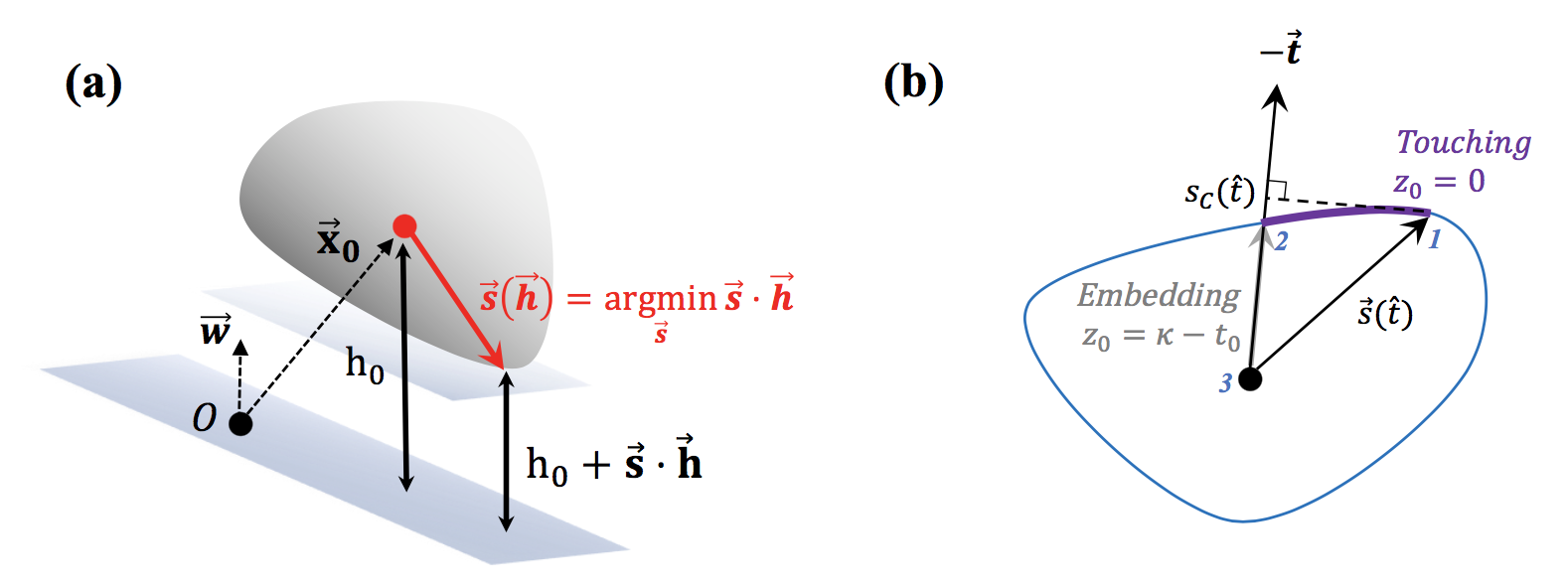
Figure 19: Geometrical Interpretation. (a) Relationship between different fields. $h_{0}=\left\|\mathbf{w}\right\|^{-1}y\mathbf{w}\cdot\mathbf{x_{0}}$: field induced by the center of the manifold $\mathbf{x}_{0}$, i.e. the distance between the center $\mathbf{x}_{0}$ and the solution hyperplane characterized by $\mathbf{w}$ . $\vec{h}$ is the vector of fields induced by basis vectors, i.e. $h_{i}^{\mu}=\left\|\mathbf{w}\right\|^{-1}y^{\mu}\mathbf{w}\cdot\mathbf{u}_{i}^{\mu}$. Together, $h_{0}+\vec{s}\cdot\vec{h}$ determines the distance between the solution hyperplane and the closest point on the manifold characterized by the manifold shape constraint $f(\vec{s})=0$. (b) Geometric interpretation of different regimes. Purple line denotes the range of$\vec{s}(\hat{t})$ when the manifold is in the touching regime, from the point 1 to point 2. From point 2 to 3 denotes the range of $\vec{s}(\hat{t})$ when the manifold is in the embedded regime.

Large D Limit

We assume that $D$ is large but the size of the manifold is such that $s\ll\sqrt{D}$,

$$\alpha_{M}^{-1}=\int D\vec{t}\int_{-\infty}^{\kappa-\vec{t}\cdot\vec{s}}Dt_{0}\frac{(\kappa-\vec{t}\cdot\vec{s}-t_{0})^{2}}{1+s^{2}},\>\text{when}\>D\gg 1$$ (250)

$$\vec{s}=\tilde{s}(\vec{t}-z_{0}\vec{s})$$ (251)

$$z_{0}=\frac{-\vec{t}\cdot\vec{s}-t_{0}}{1+s^{2}}$$ (252)

Since $\vec{t}\cdot\vec{s}$ is large we can approximate

$$z_{0}=\frac{-\vec{t}\cdot\vec{s}}{1+s^{2}}=\vec{h}\cdot\vec{s}$$ (253)

and assume self averaging,

$$z_{0}=\frac{-\langle\vec{t}\cdot\vec{s}\rangle}{1+\langle s^{2}\rangle}=\langle\vec{h}\cdot s\rangle$$ (254)

We can introduce manifold dimensions and radii,

Manifold Radius and Dimension

We can now express the above results in terms of the effective manifold dimensionality and radius. In the limit of large $D$, we can define

$$R_{M}^{2}=\langle s^{2}\rangle_{\vec{t}}$$ (255)

$$D_{M}=\frac{\langle\vec{t}\cdot\vec{s}\rangle_{\vec{t}}^{2}}{R_{M}^{2}}$$ (256)

where$\vec{s}$ is defined by the coupled equations

$$\vec{s}=\tilde{s}(\vec{t}-z_{0}\vec{s})$$ (257)

$$z_{0}=\frac{-\langle\vec{t}\cdot\vec{s}\rangle}{1+\langle s^{2}\rangle}$$ (258)

so that the capacity can be expressed as

$$\alpha_{M}=(1+R_{M}^{2})\alpha_{0}(\kappa+R_{M}\sqrt{D_{M}})$$ (259)

where $R_{M}\sqrt{D_{M}}$ behaves like an additional margin $\kappa_{M}$ introduced by the manifold structure.

Scaling Regime

In the scaling regime, $s_{i}=O(D^{-1})$ and $z_{0}$is $O(1)$ so $\vec{t}-z_{0}\vec{s}\approx\vec{t}$. In this regime, Eqns. 255-259 hold but the expression for the manifold radius and dimension are simpler, since $\vec{s}$ simply becomes

$$\vec{s}=\tilde{s}(\vec{t})$$ (260)

Here, the expressions for effective radius and dimension is given with Eqn. 260,

$$R_{W}^{2}=\langle s^{2}\rangle_{\vec{t}},\;\text{in scaling regime}$$ (261)

$$D_{W}=\frac{\langle\vec{t}\cdot\vec{s}\rangle_{\vec{t}}^{2}}{R_{M}^{2}},\>\text{in scaling regime}$$ (262)

with the excess margin

$$\kappa_{W}=R_{W}\sqrt{D_{W}}\>\text{in scaling regime}$$ (263)

where $W$ stands for widths, see Figure 20.

Mean Width

Interestingly, the excess margin $\kappa_{W}$ is related to a well known measure of a size of convex manifolds, known as the mean widths^{vershynin2015estimation}, and is defined as

$$\text{Gaussian Mean Width}=\langle\max_{\vec{s}_{1},\vec{s}_{2}\in M}\left[\vec{t}\cdot\left(\vec{s_{1}}-\vec{s_{2}}\right)\right]\rangle_{\vec{t}}\sim 2R_{W}\sqrt{D_{W}}=2\kappa_{W}$$ (264)

where $\vec{s}_{1}$ and $\vec{s}_{2}$ are points on a given manifold $M$ in $\mathbb{R}^{N}$ and $\vec{t}$ is a Gaussian random vector $\sim I(0,I_{D_{\vec{t}}})$ .

The relationship between the manifold dimension $D_{W}$ and manifold radius $R_{W}$ and Gaussian Mean Width is illustrated in Fig. 20.

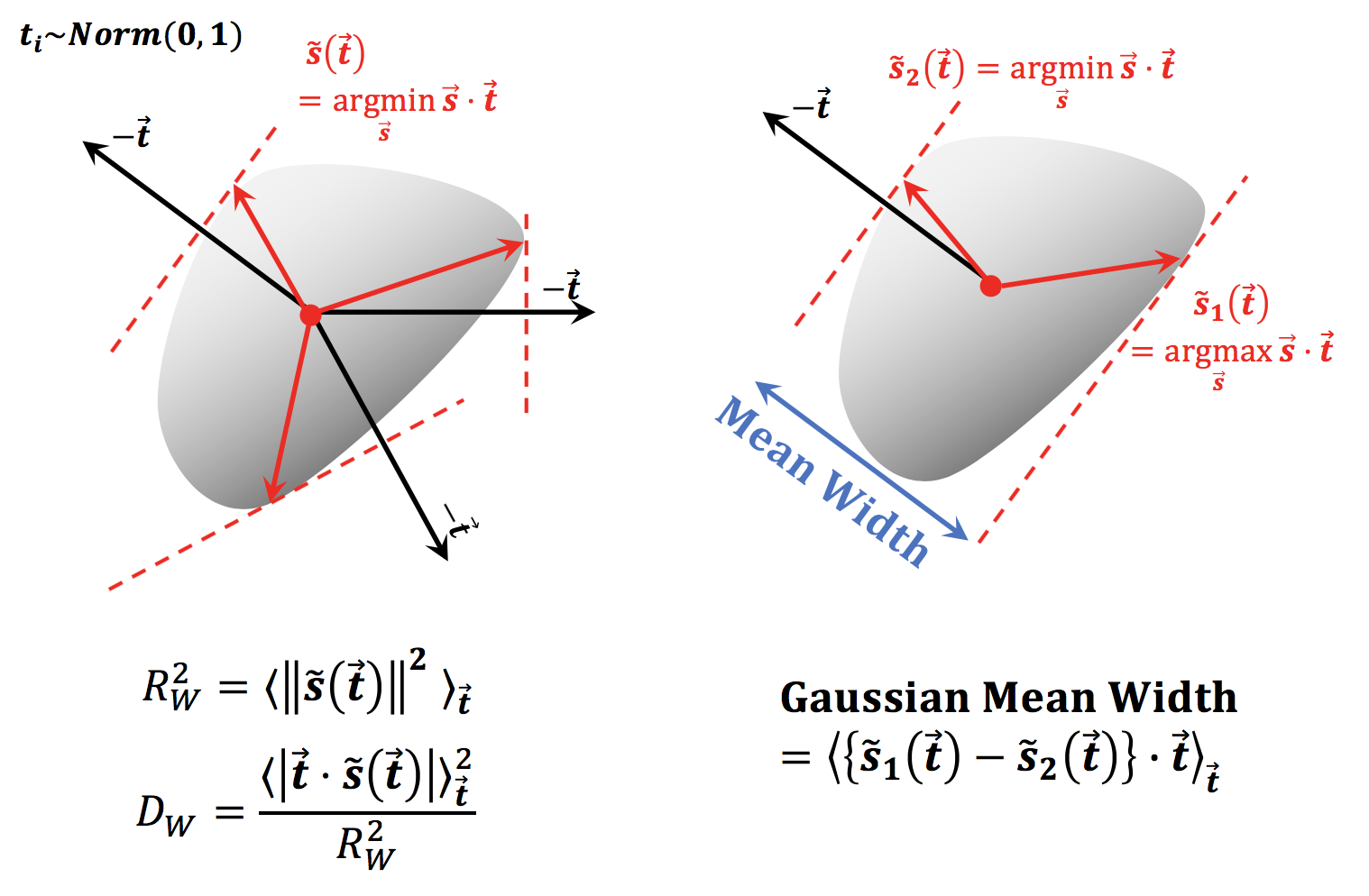
Figure 20: Relationship between the Gaussian Mean Width the Effective Manifold Radius and Dimension in the Scaling Regime. (a) Effective Radius $R_{W}=\langle\left\|\tilde{s}(\vec{t})\right\|^{2}\rangle_{\vec{t}}$ is the mean of max projection points $\tilde{s}(\vec{t})$ along the random directions $\vec{t}$, while the effective dimension $D_{W}$ is defined as $\frac{\langle\left|\vec{t}\cdot\tilde{s}(\vec{t})\right|\rangle_{\vec{t}}^{2}}{R_{W}^{2}}$. (b) Gaussian Mean Width is defined as $GMW=\langle\left\{\tilde{s_{1}}(\vec{t})-\tilde{s_{2}}(\vec{t})\right\}\cdot\vec{t}\rangle_{\vec{t}}$, and in this definition, $GMW=R_{W}\sqrt{D_{W}}$.

General Manifolds

Smooth networks are simple in that they can touch a hyperplane by a single point or be fully embedded in it. This is not true for non-smooth manifolds, as there are many facets that can be partially embedded due to the non-smoothness. In other words, a non-smooth manifold can touch the hyperplane by a point, line segment, a facet, or multiple facets (Fig. 21).

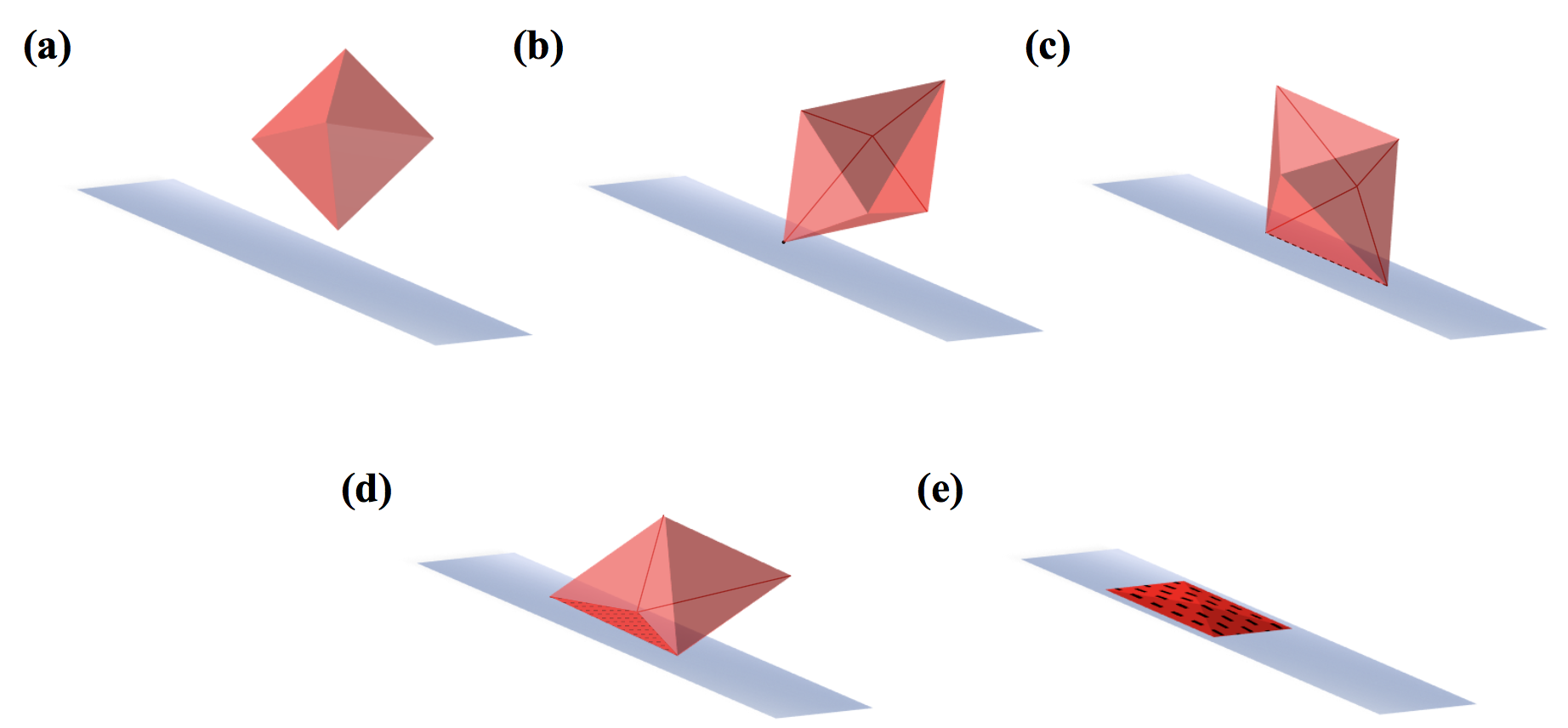
Figure 21: Embedding (support) structures of non-smooth manifolds: $L_{1}$ manifolds. (a) Interior manifolds. (b) Touching with a point. (c) Touching with a line. (d) Touching with a facet. (e) Embedded in the margin plane.

Capacity of Smooth and Non-smooth Manifolds

Given the complicated geometric relations between non smooth manifolds and the margin planes, explicit expression for the capacity that delineates the different regimes in $\vec{t}$ and $t_{0}$ is cumbersome and depends on the specific details of the manifold at hand. Here we note that for any manifold, we can write down the capacity in the following universal form

Universal mean field equation for manifold capacity $$\alpha_{M}^{-1}=\int D\vec{t}\int_{-\infty}^{\kappa-\vec{t}\cdot\vec{s}(\vec{t})}Dt_{0}\frac{(-\vec{t}\cdot\vec{s}-t_{0}+\kappa)^{2}}{1+s^{2}}$$ (265) where, $\vec{s}$ is defined via $$\vec{s}=\tilde{s}(\vec{t}-z_{0}\vec{s})$$ (266) $$z_{0}=\frac{-\vec{t}\cdot\vec{s}-t_{0}+\kappa}{1+s^{2}}$$ (267)

The key point is that the solution for $\vec{s}$ changes its nature as $t_{0}$ decreases (for a given $\vec{t}$) and automatically dissects the range of integration over $t_{0}$ to the specific domains (touching with points, lines, facets, etc). Note that the fully embedded regime is also incorporated in 265. In this regime, $\vec{t}+\vec{z}=\vec{t}-z_{0}\vec{s}=0,$ and $z_{0}=\kappa-t_{0}$, hence, $\vec{s}=\vec{t}/(\kappa-t_{0})$ , which in the embedding regime will be a point inside the convex manifold in the direction of $\vec{t}$, see Fig. 19(b).

Large $D$ Approximation for a General Manifold

In the case of smooth manifolds, we have shown that in the limit of large $D$ the capacity can be approximated by Eqns. 265-258. Here we note that the same approximation applies to general, smooth as well as non-smooth manifolds. Specifically, we approximate the capacity as

Capacity for General Manifolds in high $D$: $$\alpha_{M}=(1+R_{M}^{2})\alpha_{0}(\kappa+\kappa_{M})$$ (268) $$\kappa_{M}=R_{M}\sqrt{D_{M}}$$ (269) $$R_{M}^{2}=\langle s^{2}\rangle$$ (270) $$D_{M}=\frac{\langle\vec{t}\cdot\vec{s}\rangle^{2}}{R_{M}^{2}}$$ (271) where $$\vec{s}=\tilde{s}(\vec{t}-z_{0}\vec{s})$$ (272) $$z_{0}=\frac{-\langle\vec{t}\cdot\vec{s}\rangle}{1+\langle s^{2}\rangle}$$ (273)

and averages are over gaussian $D-dimensional$ vectors $\vec{t}$. As is the case of smooth manifolds, in the scaling regime where $R_{M}$ is $O(D^{-1/2})$, $R_{M}$ and $D_{M}$ are given via $\vec{s}$ where $\vec{s}$ is simply $\tilde{s}(\vec{t})$ , hence they coincide with $R_{W}$ and $D_{W}$ and are related to the Gaussian Mean Width as in the smooth case above (Figure 20).

Numerical Investigations

Numerical Solutions of the Mean Field Equations

In simple cases analytical expressions can be used to solve numerically the mean field equations, as is the case of ellipsoids discussed above. Here we show how to use the analytical formulae to solve the mean field equations for the ellipsoids. For a general manifold, calculating $\vec{s}\cdot\vec{t}$ and $s^{2}$ for $\vec{s}$ on the manifold for each $\vec{t}$ and $t_{0}$ can be done by iterative methods. Here we present such an algorithm, adequate for general manifolds in the large $D$ regime. In the limit of large $D$, $\left|\vec{t}\cdot\vec{s}\right|\gg\left|t_{0}\right|,\kappa$, and we can use Eqns 268-273. Furthermore, in this limit, $\vec{t}\cdot\vec{s}$, and $s^{2}$ are self averaged with respect to $\vec{t}$. The pseudocode for the algorithm is given in Alg. 4 below.

Iterative Numerical Solution

In order to solve for $s$ and $z_{0}$ (Eqn 272- 273), we use an algorithm for each $\vec{t}$, that essentially iterates between updating $z_{0}$ given the current estimate of $\vec{s}$, using Eqn 273 and updating the estimate of $\vec{s}$ given the new estimate of $z_{0}$ and the current estimate of $\vec{s}$, Eqn 272.

Solving eq. 272: First we note that evaluating the $min$ operation in Eqn 272 can be done explicitly in simple cases (in particular, for convex smooth manifolds with known parametrization). In general, one can search numerically for the max projection points (or signed min projection points). If the manifold is non-smooth and has a finite number of vertices, then one can simply iterate over all vertices. Otherwise, a local search using a gradient can be done, and since the search is on the convex hull, the local search guarantees the convergence to the global optimum. This appears as a $maxproj$ function in Alg. 4.

Note that $\vec{s}$ we are solving is not simply a max projection point on $\vec{t}$, but a max projection on $\vec{h}=\vec{t}-z_{0}\vec{s}$ (Eqn. 272). The solution $\vec{s}$ may come from anywhere inside of the convex hull or the surface of the manifold, hence we allow the search on$\vec{s}$ to be a linear combination of the vertices. To search for $\vec{s}$, in the next step we define $\vec{s}_{k}=\eta\vec{s_{h}}+(1-\eta)\vec{s}_{k-1}$ which is a linear sum of $\vec{s}_{k-1}$ in the previous step $k-1$ and the max projection in the direction of $\vec{h}$ at time $k$, $\vec{s}_{h}$. If the difference between $\vec{s_{k}}$ and $\vec{s}_{k-1}$ is smaller than a given tolerance $\epsilon_{0}$, then $\vec{s}$ converged, as well as $z_{0}$. Otherwise, continue to the $k+1$ th step, where the new $\vec{h}$ is computed with the new $\vec{s}$. The algorithm for this is summarized in the pseudocode (Alg. 4).

[$\alpha_{M}$,$R_{M}$, $D_{M}$] = function manifold_capacity($D$, $n_{t}$,$\eta$, $n_{max}$ , $\epsilon_{0}$, $S$)

Input: {Manifold dimension $D$, number of $t^{\prime}s$ $n_{t}$, learning rate $\eta$, max iteration $n_{max}$, tolerance $\epsilon_{0}$, the manifold data$S$ defined in $\mathbb{R}^{D\times M}$}

for i=1 to$n_{t}$ do

 $\vec{t}=\vec{t}^{(i)}\sim Norm(0,\mathbb{I}_{D}])$

 Set $k=0$, $\epsilon_{ts}=\infty$

 $\vec{s}_{k}=maxproj(\vec{t}$,$S$)

 while $k<n_{max}$ and $\epsilon_{s}>\epsilon_{0}$

   $k=k+1$

   $z_{0}=\frac{-\vec{t}\cdot\vec{s}}{1+s^{2}}$

  $\vec{h}=\vec{t}-z_{0}\vec{s}$

  $\vec{s}_{h}=maxproj(\vec{h},S)$

  $\vec{s_{k}}=\eta\vec{s_{h}}+(1-\eta)\vec{s}_{k-1}$

  $\epsilon_{s}=||\vec{s}_{k}-\vec{s}_{k-1}||/||\vec{s}_{k}||$

 end

 $\vec{s}^{(i)}=\vec{s}_{k}$

end

$R_{M}=sqrt\left\{\langle\left\|\vec{s}^{(i)}\right\|^{2}\rangle_{i}\right\}$

$D_{M}=\frac{\left\{\langle\vec{t}^{(i)}\cdot\vec{s}^{(i)}\rangle_{i}\right\}^{2}}{R_{M}^{2}}$

$\alpha_{M}=(1+R_{M}^{2})\alpha_{0}(\kappa+R_{M}\sqrt{D_{M}})$

Output = [$\alpha_{M}$,$R_{M}$, $D_{M}$]

Algorithm 4 Iterative method for approximating capacity of general manifolds in high $D$

In the following sections, we show the specific manifold examples and how the input $S$ of $maxproj(\vec{t},S)$ , as well as the details of the max projection search differ based on the type of the problem.

Simulation Results

Ellipsoids

Consider the ellipsoids give by Eqn. 157 and constraint, Eqn. 159. In this case, the manifold parameterization is known, then $\vec{s}_{k}=\underset{\vec{s}}{\text{argmax}}\vec{t}\cdot\vec{s}$ has an analytical solution given by the minus of Eqn. 163 and Eqn. 164 for ellipsoids. In this case, the input to the max projection operation for ellipsoid, called $maxproj^{ellipsoid}$should include the radii vector. Pseudocode for $maxproj^{ellipsoid}$ is given in Alg. 5. Furthermore, in the case of ellipsoids, it is possible to solve for $z_{0}$ analytically in the of the large $D$ (i.e. Eqn.195). However, to test the effectiveness of the iterative algorithm, we proceed to test the iterative algorithm in the simulations below.

$\tilde{s}$ = function $maxproj^{ellipsoid}(\vec{t},S)$

Input: $D$-dimensional direction vector $\vec{t}$, $S=\{\text{$D$-dimensional radii vector }\vec{R}\}$

for i=1 to$D$ do

$\tilde{s}_{i}=\frac{t_{i}R_{i}^{2}}{\sqrt{\sum_{j}t_{j}^{2}R_{j}^{2}}}$

end

Output: The point on the manifold with max projection in $\vec{t}$ , $\tilde{s}$

Algorithm 5 Maximum Projection Point on Ellipsoid $S$

Using the iterative methods described above, we calculated the theoretical estimate of linear classification capacity of ellipsoids, with embedding dimension $D=50$ in ambient dimension $N=100$ . The radii for each ellipsoid is given by the $R_{i}=Unif[0.5R_{0},1.5R_{0}]$ for each $i=1,...,D$ . $R_{0}$ is shown in the $x$ axis of the Fig 22 as $\langle R_{i}\rangle_{i}$. We compare the capacity estimated by the iterative algorithm using the mean field approximation (noted as $\alpha_{iter}$), with the capacities estimated by the expressions of effective radius and effective dimension in different regimes (in the regime of $R_{i}\sim O(1)$, Eqns. 200-201, and in the scaling regime, Eqns 210-211. We also calculated the simulation capacity in the similar manner to $M_{4}$ algorithms for $L_{2}$ balls described in Chapter Linear Classification of Spherical Manifolds-The Maximum Margin Manifold Machines, with the worst point analytically calculated by Eqn. 163-164. Using the ambient dimension of $N=100$ for the ellipsoids, the critical value of $P$ was determined by finding the value of $P$ such that the average number of being separable was half the times of the total number of $50$ repetitions.

The iterative algorithm capacity matches the estimated capacities using effective radii and dimensions well, as well as simulation capacities described above. In the limit of large $R_{i}$, the capacity approaches $1/D$, where the hyperplane is orthogonal to all embedded dimensions of an ellipsoid.

We also compare the measures of dimensions relevant for the classification capacity of ellipsoids (Fig. 22). The dimensions calculated from the iterative algorithm ($D_{M}$, M for manifolds) is compared with the approximate effective ellipsoid dimensions $D_{E}$ in different regimes (Eqn 201 and 211), and they agree well. Furthermore, these estimated effective ellipsoid dimensions match the participation ratio (214), $D_{svd}$ , when $R_{i}$ is in the scaling regime, and match the actual full embedding dimension $D$ when $R_{i}$ is large. Intuitively, this means that $D_{svd}$ is a relevant measure for linear classification capacity when $R_{i}$’s are small ($\sim D^{-1/2}$). In the case where $R_{i}$ is large, the embedding dimension $D$ is the relevant measure for the capacity, because the solution has to orthogonalize all embedding dimensions independent of the structure.

We also compare the ratio between effective radius and the actual scale of the ellipsoid (in this case $R_{0}=\langle R_{i}\rangle_{i}$), for $R_{M}$ calculated from the iterative algorithm and $R_{eff}$ calculated from approximations in each regime of $R_{i}\sim D^{-1/2}$ (scaling) and $R_{i}\sim O(1)$ (Fig. 22). As before, the agreement between the $R_{M}$, $R_{eff}$’s are good. Furthermore, the ratio between effective radius (for capacity) and the mean of the radii start out above 1, and decreases with increasing $R_{0}$ . This means that the larger the ellipsoids get, the more fraction of ellipsoids get embedded, hence effective radius $R_{eff}$ contributing to the effective increase in the margin $\kappa_{eff}=R_{eff}\sqrt{D_{eff}}$ gets smaller due to the embedding configuration.

Figure 22: Linear Classification of Ellipsoids. (a) Linear Classification Capacity of $D$-dimensional ellipsoids, $\alpha_{E}=P/N$, where $N$ is the ambient dimension, and $P$ is maximum the number of ellipsoids such that $P$ ellipsoids are linearly separable. The embedding dimension of ellipsoids used was $D=50$ and $R_{i}\sim Unif\left[0.5R_{0},1.5R_{0}\right]$ for $i=1,...,D$ and $R_{0}=\langle R_{i}\rangle_{i}$ is shown in the $x$-axis. (Red) Mean field approximation capacity $\alpha_{iter}$ , evaluated by the iterative algorithm given in Alg. 4 and Alg. 5. (Blue dashed) Approximation of the ellipsoid capacity as the capacity of a ball using a large $D$ and $R_{i}\sim O(1)$ approximation for $R_{E}$ and $D_{E}$ given by Eqns. 200- 201. (black dashed) Ellipsoid capacity approximated using $R_{E}$and $D_{E}$ approximation when $R_{i}$ is in the scaling regime, given by Eqns. 210-211. (Green) Capacity approximation for large $R_{i}$, $1/D$, where all of the ellipsoid embedding dimensions are orthogonalized by the solution. (Yellow) Simulation capacity computed with $N=100$ and $50$ repetitions. (b) Dimensions of the ellipsoid. (Blue) Embedding dimension $D$. (Red) Dimension of the ellipsoid evaluated by the iterative algorithm, $D_{M}$. (Orange) Participation ratio, $D_{SVD}$, given by Eqn. 214 using $R_{i}$ as eigenvalues. (Pink) $D_{E}$ approximation in large $D$ $R_{i}\sim O(1)$ regime given by Eqn.201 (Green) $D_{E}$ approximation in large $D$ and scaling regime given by Eqn. 211. (c) Size (Radius) of Ellipsoids. (Red) Effective manifold radius $R_{M}$ evaluated by the iterative algorithm, divided by the overall scale $\langle R_{i}\rangle_{i}$. (Pink) $R_{E}$ approximation in large $D$, $R_{i}\sim O(1)$ regime given by Eqn. 200(Green) $R_{E}$ approximation in large $D$ and scaling regime given by Eqn. 210

$D$ Dimensional $L_{1}$ Manifolds

Consider the problem of linearly classifying $P$ of $D$-dimensional $L_{1}$ manifolds where the point on the $L_{1}$ manifold is given by Eqn. 157 where $f(\vec{s})=\sum_{i=1}^{D}|s_{i}/R_{i}|-1=0$ . The explicit expression for classifying $L_{1}$ manifolds is considered in ^{chung2016linear}, and in this section we focus on finding their perceptron capacity as an example of manifolds that are defined by their vertices (Fig. 21). In this case, there are only $2D$ vertices (2 extreme points along the direction vector $\mathbf{u}_{i}$), and finding the max projection point in the direction of $\vec{t}$ from the set of points $S$ is given by $\vec{s}_{k}=\underset{l}{\text{argmax}}\vec{t}\cdot S_{l}$ , simply the search over all $2D$ vertices whose computation time is linear in the number of points. In this case, the input for the max projection operation in the iterative algorithm, called $maxproj^{setpoints}$, should include the set of points. Pseudocode for $maxproj^{setpoints}$ is given by Alg. 6.

$\tilde{s}$ = function $maxproj^{setpoints}(\vec{t},S)$

Input: $D$-dimensional direction vector$\vec{t}$, A set of $M$ points in $D$ dimensional basis which define the vertices of the convex hull$S=\{X\in\mathbb{R}^{D\times M}\}$

$i_{l}=argmax_{l}\vec{t}\cdot X(:,l)$

$\tilde{s}=X(:,i_{l}$)

Output: The point on the manifold with max projection in $\vec{t}$ , $\tilde{s}$

Algorithm 6 Maximum Projection Point on a set of points $S$

Using the iterative methods described above, we calculated the linear classification of capacity of $L_{1}$ manifolds, with the embedding dimension $D=20$ in the ambient dimension $N=100.$ The radii for each direction is set to be equal, i.e. $R_{i}=R$ (all vertices are distance $R$ away from the center ) for all $i=1,...D$. $R$ is shown in the x axis of the Fig. 23.

We compare the capacity estimated by the iterative algorithm using the mean field approximation (noted as $\alpha_{Iter}$), with the capacities estimated as that of a ball using the effective radius and effective dimension of $L_{1}$ manifolds in the scaling regime. In the scaling regime, the replica analysis gives us $R_{M}=R$ and $D_{M}=2\text{log}(D)$, and the derivations are given in the appendix to the chapter (section Effective Dimension of $L_{1}$ manifolds). The estimated capacity using the iterative algorithm agrees well with the simulation capacity, as well as approximations in the scaling regime, and large R regime.

We also compare the measures of dimensions relevant for the classification capacity of $L_{1}$ manifolds. The dimension estimated by the iterative algorithm matches the approximation of $D_{M}(L_{1})\sim 2\text{log}(D)$ in the scaling regime (due to the extreme value theory, details in the Appendix to the chapter), and in the regime of large $R$ it matches the embedding dimension $D$, which in this case is equivalent to the participation ratio $D_{svd}$ (as all $R_{i}=R$ ).

Furthermore, in the scaling regime, the effective manifold radius found by the iterative algorithm $R_{M}$ is close to $R$, as predicted by the theory (details in the appendix). $R_{M}/R$ transitions from 1 (in the scaling regime) to a value much smaller than 1 (in the large $R$ regime), due to the increased fraction of $L_{1}$ manifolds that are embedded.

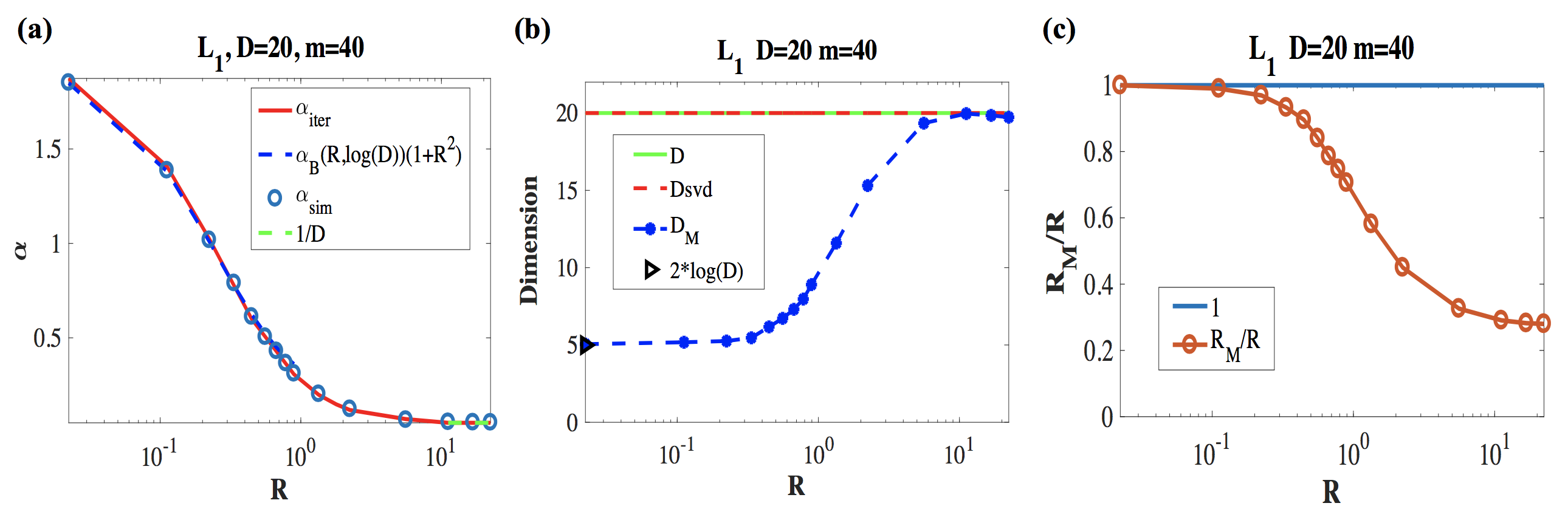
Figure 23: Linear Classification of Non-smooth manifolds: $D$-dimensional $L_{1}$ Manifolds of Radius $R$. (a) Linear Classification Capacity of $D$-dimensional $L_{1}$ manifolds, $\alpha=P/N$, where $N$ is the ambient dimension, and $P$ is the maximum number of manifolds such that $P$ $L_{1}$manifolds are linearly separable. The embedding dimension of $L_{1}$manifolds used was $D=20$ and the number of subsamples used for testing was $m=40$, two endpoints in each basis vector direction. $R$ is shown in the $x$-axis. (Red) Mean field approximation capacity $\alpha_{iter}$ , evaluated by the iterative algorithm given in Alg. 4 and Alg. 6. (Blue dashed) Approximation of the $L_{1}$ capacity as the capacity of a ball using $R$ as the actual $R$ and $D_{M}=\text{log}D$, which is the approximation of effective manifold properties in the large $D$ regime. (blue markers) Simulation capacity calculated with $N=100$ and $50$ iterations to compute the fraction of linear separability. (Green) Capacity approximation for large $R$, $1/D$, where all of the $L_{1}$ manifold embedding dimensions are orthogonalized by the solution. (b) Dimensions of the $L_{1}$ manifolds. (Green) Embedding dimension $D$. (Red dashed) Participation ratio, $D_{SVD}$, given by Eqn. 214 using $R_{i}=R$ as eigenvalues. (Blue) Dimension of the $L_{1}$ manifolds evaluated by the iterative algorithm, $D_{M}$. (Black marker) $D_{B_{1}}$ approximation in large $D$ regime, $2\text{log}D$ (Derivation in appendix). (c) Size (Radius) of $L_{1}$ manifolds divided by $R$. (Red) Effective manifold radius $R_{M}$ evaluated by the iterative algorithm, divided by $R$, compared with unity (Blue).

Random Strings

Consider the problem of linearly classifying $P$ of random strings, whose intrinsic dimension is 1, but the embedding dimension is $D$, and the ambient dimension of $N$ . Each point on the random string is parameterized by the vector $\vec{s}$ whose components are

$$s_{2k}=R_{k}cos\left\{k\left(\theta-\phi_{k}\right)\right\};$$ (274)

$$s_{2k+1}=R_{k}sin\left\{k\left(\theta-\phi_{k}\right)\right\}$$ (275)

This can be re-written as

$$x_{i}^{\mu}=\left(x_{0}\right)_{i}^{\mu}+\sum_{n=1}^{D/2}R_{n}e^{jn(\theta-\phi_{n})}u_{i}$$ (276)

(where the $j$ is used as an imaginary $\sqrt{-1}$ to distinguish from the index $i$ ).

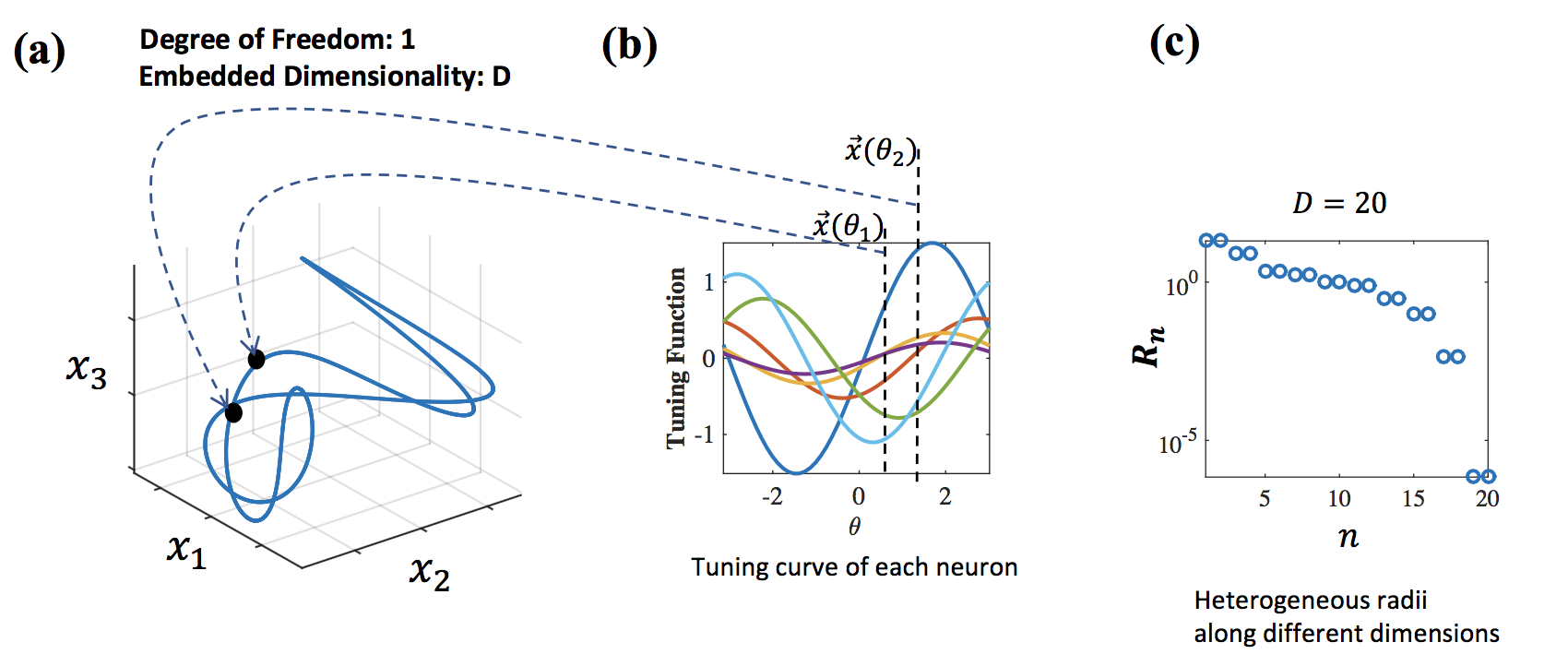
Figure 24: Random Strings (Illustration). (a) Random String in Neural State Space. The values in each ambient dimension is given by each neuron’s activity. The random string’s degree of freedom is 1, while the embedding dimension is $D$. Each point on the sample manifold represents neural activity of a same object, with different latent variable such as orientation of an object. (b) Neural Interpretation of Random Strings. The random string manifolds given by Eqns. 274-276 can be interpreted as orientation tuned neurons with different amplitudes and frequencies. (c) Illustration of $R_{n}$ for $n$th basis vector, which is similar to the amplitude of the neural tuning curve for $n$ th neuron.

Figure 24 illustrates an example of a random string. This definition has an interesting analogy with the activity patterns of the population of orientation tuned neurons. For instance, the value of point $\mathbf{x}$ in $i$ th dimension, $x_{i}$ can be thought of as $i$ th neuron’s activity, where each neuron is tuned to a different orientation (middle panel). The heterogenous $R_{i}$ can be thought of as different amplitudes of the neural activity. In this analogy, if you take an object at one angle, then all neurons will have different levels of activations, and the slice of the activity patterns correspond to a point on a random string, parametrized by $\theta$, which is essentially the angle of an object. If you change the orientation of the stimulus, then the activity patterns correspond to a different slice, which corresponds to a different point on a $\theta$-parametrized random string. Once you rotate the stimulus the full $360\mathring{}$, then the activity pattern comes back to the original slice, and you come back to the original point on the random string. Note that this particular random string lies on the surface of a ball, whose radius is $R_{string}=\sqrt{\sum_{n=1}^{D/2}R_{n}^{2}}$.

What should be an effective dimension of this string with heterogenous scales $\vec{R}$? And, if these strings are in random positions and directions, what should be their capacity? To test this, we calculated the classification capacity of samples of random strings in embedding dimension $D$, ambient dimension $N=100$, where the number of samples used was $m=200$, such that $\theta_{m}=\frac{2\pi}{m}$, and $R_{n}=R$ for all $n$.

Figure 25: Linear Classification of $D$-dimensional Random Strings. (a) Linear Classification Capacity of $D$-dimensional Random Strings, $\alpha=P/N$, where $N$ is the ambient dimension, and $P$ is the maximum number of random strings such that $P$ random strings are linearly separable. The embedding dimension of random strings used was $D=20$ and the number of subsamples used for testing was $m=200$. $R_{string}$, overall scale of the random string, and the radius of the $D$-dimensional ball that the random string is on, is shown in the $x$-axis. (Red dashed) Mean field approximation capacity $\alpha_{iter}$ , evaluated by the iterative algorithm given in Alg. 4 and Alg. 6. (Yellow marker) Simulation capacity calculated with $N=100$ and $50$ iterations to compute the fraction of linear separability. (b) Dimensions of the Random Strings. (Green) Embedding dimension $D$. (Red dashed) Participation ratio, $D_{SVD}$, given by Eqn. 214 using $R_{i}=R$ as eigenvalues. (Blue) Dimension of the random strings evaluated by the iterative algorithm, $D_{M}$. (Black marker) $\text{1+log}D$. (c) Size (Radius) of random strings divided by $R$. (Red) Effective manifold radius $R_{M}$ evaluated by the iterative algorithm, divided by $R$, compared with unity (Blue).

We find that the classification capacity $\alpha_{M}=\alpha_{iter}$ found by an iterative algorithm matches the simulation capacity of random strings (Figure 25(a)). In the case of random strings, the manifold effective dimension $D_{M}$ (also found via the iterative algorithm) has a very low effective dimension in the scaling regime, due to the fact that it is a string whose intrinsic dimension is merely $1$ and is not filling the space spanned by $D$ basis vectors, although when $R$ is large, the solution has to orthogonalize the manifolds and the effective dimension approaches the embedding dimension $D$, and it is reflected in the $D_{M}$ found via the iterative algorithm (Figure 25(b)). Note that in this case, since all $R_{i}$ has the same size, $D_{svd}=D$ . Furthermore, $R_{M}$ is $R$ in the scaling regime, and $R_{M}$goes to a value much smaller than $R$ in the large $R$ regime, reflecting the fact that many of the random strings must be orthogonalized by the solution, and therefore more of them are embedded, resulting in smaller $R_{M}/R$ seen by the centers.

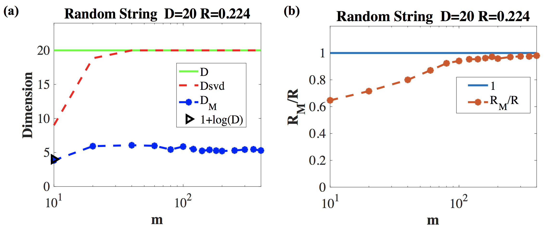
Figure 26: Effective Properties Random Strings for Different Number of Samples Per Manifold. (a) Random String Dimension versus the Number of Samples Per Manifold ($m$), for $N=100$, $D=20$, $R=0.224$($\leavevmode\nobreak\ 1/\sqrt{D})$). Both participation ratio, $D_{svd}$ (red) and the effective manifold dimension found by the Mean Field iterative algorithm, $D_{M}$, saturates around $m=50$, indicating that $m=200$ used in the Figure 25 is already a saturated, $m$ -independant properties. (b) Random String Radius versus the Number of Samples Per Manifold (m). The effective manifold radius ($R_{M}$) found by the Mean Field iterative algorithm saturates around $m=100$.

In the simulations for Figure 25, we used $m=200$ training samples per each manifold. In the above figure we find that the manifold dimensions $D_{M}$and radius $R_{M}$ is in the saturated regime as a function of $m$, due to the fact that the samples are coming from a string, and the sampling is already dense at $m=200.$ This is essentially like doing a local search for the worst points (although not explicit), because we are in the densely sampled regime.

Discussion

We have presented a mean field theoretic calculation of linear classification of general manifolds, extending Gardner’s replica theory of classification of random isolated points^{gardner87, gardnerEPL} and the recently developed theory of classification of random balls ^{chung2016linear}. This theory characterize the capacity as the inverse rate of reduction in the entropy of the weight vector space by the separability constraints per manifold. These constraints are expressed in terms of special points on the manifolds that have minimum projections on self consistent $D-$dimensional field vector. Importantly, we were able to derive a set of universal mean field equations applicable to all low dimensional convex manifolds, 265-267. The key point is that for a given manifold geometry, the position of the worst point on the manifold represented by $\vec{s}=\tilde{s}(\vec{t}-z_{0}\vec{s})$ changes as the field on the center represented by $t_{0}$ spanning the sequence of increasingly large overlap between the manifold and the the margin plane. This sequence depends of course on the details of the geometry of the convex manifold. These equations cannot be solved analytically except for the simplest geometries. We have developed an iterative algorithm to solve these self consistent equations, and in our experience, their converge is remarkably fast even when dealing with $D$ dimensional manifolds with $D$ in the range of $10-100$.

Of particular interest is the case of manifolds with high dimension ($D\gg 1$) In this case, the key parameters are Manifold Radius, $R_{M}$ and Dimensionality $D_{M}$. The manifold capacity is equivalent to that of $L_{2}$ balls with dimensionality and radius equal to $D_{M}$ and $R_{M}$ respectively. These quantities appear in the capacity mainly through the excess margin $\kappa_{M}=R_{M}\sqrt{D_{M}}$. The reason for this combination is the following. Consider first, an $N$ dimensional ball. The margin is not dimensionless but depends on the norm of the inputs. Thus, if we demand a margin $\kappa$this is equivalent to demanding a margin $\kappa+R\sqrt{N}$from the centers, since, if the distance of the points on the circumference of the ball from the center is $R\sqrt{N}$. Now when the ball is low dimensional, a reduction in the required excess margin occurs due to the tilt of the ball with respect to the hyperplane, so that the projection of the center should increase only by a factor $N\sqrt{D/N}=R\sqrt{D}$. A similar argument holds for a general manifold in this limit.

We have noted that the geometric parameters $R_{M}$ and $D_{M}$ are not intrinsic geometric measures but depend also on the overall size of the manifolds relative to the center norm. Thus, if the manifold is increased by scaling all the points by a global factor, say $r$, relative to the center, then when $r$ grows, eventually $D_{M}$ approaches the full embedding dimension $D$, reflecting the need of a solution to be orthogonal to the entire manifold subspace. Conversely, when $r$ decreases, eventually the manifold reaches the scaling regime where capacity is finite despite the high dimension, and $R_{M}\sqrt{D_{M}}$ approach the Gaussian Mean Width value $R_{W}\sqrt{D_{W}}=0.5MW$ , see 20 The change in the Manifold Dimension as $r$ increases may be dramatic. For instance, in the random string example (as well as $L_{1}$balls), $D_{M}$ increases from $D_{M}\sim\log D$ for small $r$ (the scaling regime) to $D_{M}=D$ for large $r$, see 25b.

In conclusion, the generality of the theory developed in this Chapter opens the door for applications of the derived results and methods for the investigation of neuronal representations of perceptual manifolds in biological as well as artificial neuronal networks. However, in order to do so, some limitations of the current theory might need to be relaxed. For instance, the present results deal with random labels where the two classes are of roughly equal size. In many real problems this may not be the case. Another issue is the assumption of random orientation of the manifolds. It would be important to understand the role of correlation between the manifolds. Also, it will be interesting to explore extensions to manifold representations which are not linearly separable. These issues and others are discussed in the next Chapter.

Appendix

Equivalence between $R_{i}$ and $\lambda_{i}$

Lemma 12.

If $\langle s_{i}^{2}R_{i}^{-2}\rangle=\frac{1}{D}$ then, $R_{i}\propto\lambda_{i}$.

Proof.

From the definition we know that $\langle s_{i}^{2}\rangle=\frac{R_{i}^{2}}{D}$. Consider the covariance $C$ of the manifold data $X$ from many realizations of $\vec{s}$

$$X=\mathbf{x}_{0}+\sum_{i}s_{i}\mathbf{u_{i}}$$

Then,

$$C=\langle\left\{X-\langle X\rangle\right\}\left\{X-\langle X\rangle\right\}^{T}\rangle=\sum_{ij}\langle s_{i}s_{j}\rangle\mathbf{u}_{i}\mathbf{u}_{j}^{T}$$

$\lambda_{i}$ are by definition,

$$\frac{1}{N}\lambda_{i}^{2}=\langle s_{i}^{2}\rangle$$

Hence,

$$\lambda_{i}^{2}=\frac{N}{D}R_{i}^{2}$$

∎

Effective Dimension of $L_{1}$ manifolds

In the scaling regime, $\vec{s}(\vec{t})$ for $L_{1}$ manifolds is the $i$-th vertex where $i\underset{i}{=\text{argmax}\>t_{i}}$. So, $\vec{s}\cdot\vec{t}=R\underset{i}{\text{max}\>t_{i}}$. Given $D$ normally distributed $t_{i}$’s, the max value is centered in large $D$

$$\underset{i}{\text{max}\>t_{i}}\sim\sqrt{2\log D}$$ (277)

due to the extreme value theory. Hence, we obtain

$$D_{M}=2\log D$$ (278)

$$R_{M}=R$$ (279)

for $L_{1}$ manifolds in the scaling regime.

Extensions

Correlated Manifolds

So far, we have considered randomly oriented manifolds. In real world data we expect that the manifolds will be correlated; in particular, that the subspaces spanned by the different manifolds will be partially aligned. We first consider the simple case of $D$ dimensional spheres that all share the same subspace in the ambient dimension $\mathbb{R}^{N}$.

Parallel Spheres

Consider a perceptron classifying parallel $D$-dimensional discs, embedded in $N$ dimensions. The training data is given by:

$$\mathbf{x_{0}}^{\mu}+R\sqrt{\frac{1}{D}}\sum_{i=1}^{D}\mathbf{u}_{i}s_{i}\quad\forall\left|\vec{s}\right|^{2}\leq 1$$ (280)

where as before the components of $\mathbf{x_{0}}^{\mu}$ and $\mathbf{u}_{i}$ are i.i.d. normally distributed random variables. For reasons that will be clear later on, it is convenient to scale $R$ to $R/\sqrt{D}.$ It is also convenient to rotate the axes so that $\mathbf{u}_{i}$ are along the standard first $D$ axes, so that the corresponding fields are

$$h^{\mu}(\vec{s})=\frac{1}{\sqrt{N}}y^{\mu}\left(\mathbf{w}^{T}\mathbf{x}_{0}^{\mu}+R\sqrt{\frac{N}{D}}\sum_{i=1}^{D}w_{i}s_{i}\right)>0\quad\forall\left|\vec{s}\right|^{2}\leq 1$$ (281)

where here we restrict ourselves to zero (fixed) margin.

Minimizing with respect to $s_{i}$, we get

$$s_{i}=-y^{\mu}w_{i}/\sqrt{\sum_{j}w_{j}^{2}}$$ (282)

Therefore, the minimum of LHS of 281 is

$$\min_{s}h^{\mu}(s)=\frac{1}{\sqrt{N}}y^{\mu}\mathbf{w}^{T}\mathbf{x}_{0}^{\mu}-R\sqrt{\frac{1}{D}\sum_{i=1}^{D}w_{i}^{2}}$$ (283)

Thus, the constraints are reduced to

$$\frac{1}{\sqrt{N}}y^{\mu}\mathbf{w}^{T}\mathbf{x}_{0}^{\mu}>\kappa_{\rho}$$ (284)

where

$$\kappa_{\rho}=R\sqrt{\rho}$$ (285)

and

$$\rho=\frac{1}{D}\sum_{i=1}^{D}w_{i}^{2}$$ (286)

which is an average of dot products between the solution $\mathbf{w}$ and direction vectors (in a rotated coordinate). Let us call $\rho$ the overlap parameter.

Note that the total variance of each manifold is $R^{2}N/D$ while the square distance between center pairs is: $2N$. Thus, their ratio is $R^{2}/2D$ . In contrast, in the random spheres, the total variance of each manifold is $R^{2}N$ whereas the square distance is as before $2N$ . Hence the ratio is $R^{2}/2$ .

It is important to note that if $D\ll N$ then the solution vector $\mathbf{w}$ can be orthogonal to all manifolds by zeroing the corresponding $D$ components for any size of the manifold $R$, without sacrificing significant degrees of freedom. In this case, we expect the capacity to be the same as for the capacity with the centers only, in the reduced dimension of $N-D$.

Thus, the problem of parallel manifolds is interesting only when $D\approx N$ ($D$ scales with $N$). Let us define the relative dimension parameter $d$, such that

$$D=dN$$ (287)

In this regime, zeroing all $D$ components of $\mathbf{w}$ is costly, so we expect that the nature of $\mathbf{w}$ depends on $d$ and $R$. Note that in this case (since $D\gg 1$) the relevant scale of the radius should be radius over $\sqrt{D}$. In our normalization above it means that $R$ is of order $1$.

Capacity

The basic constraint 284 is equivalent to a Gardner’s theory with margin $\kappa$ which however is not a fixed parameter but assumes self consistent value, set by the order parameter $\rho$ which measures the overlap between $\mathbf{w}$ and the manifold subspaces. To evaluate $\rho$ (Eqn. 286) we need to evaluate the entropy of the solution space given the constraint that the solutions’ average projection on the common manifold subspaces is $\rho$ . We denote this entropy (per $N$) by$S_{0}(\rho)$. The analog of 175 is

$$\frac{1}{N}\langle\log V\rangle=S_{0}(\rho)-\alpha\alpha_{0}^{-1}(\kappa_{\rho})$$ (288)

where $\alpha_{0}$ refers to the capacity for points. As before, in the capacity limit, $\langle\log V\rangle$ vanishes and from 288 it follows that the capacity is

$$\alpha_{||}=\alpha_{0}(\kappa_{\rho})S_{0}^{-1}(\rho)$$ (289)

where the symbol $||$ stands for parallel manifolds and the entropy term is

$$S_{0}(\rho)=\frac{dx^{2}}{(x-1+d)^{2}+d(1-d)}$$ (290)

where $x$ is related to $\rho$ through,

$$\rho=\frac{(x-1+d)^{2}}{d[(x-1+d)^{2}+d(1-d)]}$$ (291)

Different overlap $\rho$ yields different capacities, so optimizing the capacity $\alpha_{||}$ with respect to $\rho$ yields the following equation (for $\rho$ or $x$), as $\alpha_{||}$ is the maximum possible capacity

$$\frac{x(1-x)\sqrt{d}}{\sqrt{(x-1+d)^{2}+d(1-d)}}=\alpha_{||}R\left(\kappa_{\rho}H(-\kappa_{\rho})+\frac{\exp-\frac{1}{2}\kappa_{\rho}^{2}}{\sqrt{2\pi}}\right)$$ (292)

Since there are 3 equations (Eqns 289-290, 291 and 292), and 3 unknowns ($\alpha_{||}$, $x$ , $\rho$), one can solve for $\alpha_{||}$ or $\rho$.

Phase Transition

The solution for the capacity above shows dependence on the overlap parameter $\rho$, which needs to be solved via $x$ as a function of $R$. It turns out that there are two regimes of solutions for $\rho$, one where $\rho$ decreases with increasing $R$, up to $R<R_{c}$, and another where $\rho=0$ for $R>R_{c}$. Qualitatively, this means that for the parallel manifolds whose radii are smaller than $R_{c}$ , the overlap between $\mathbf{w}$ and manifold subspace is nonzero, and the overlap increases with increasing $R$. However, when the manifold $R$ is beyond a critical value $R_{c}$, all manifold subspaces are orthogonal to $\mathbf{w}$ and the overlap becomes $0$, due to the tradeoff between orthogonalizing and sacrificing the degrees of freedom. The geometric intuition for two different phases is given in Fig. 27 (a)-(b).

Let us consider the value of $R_{c}(d)$ such that $\rho=\kappa\rightarrow 0$ as $R\rightarrow R_{c}^{+}$. At this value, the solution must be orthogonal to the manifold, therefore $\alpha=2(1-d)$ (Fig. 27(c), Regime $R>R_{c}$ ). Also, for $\rho$ to vanish, $x=1-d$, yielding,

$$R_{c}(d)=\sqrt{\frac{\pi d^{2}}{2(1-d)}}$$ (293)

Thus for $R>R_{c}(d)$, $\alpha_{||}=2(1-d)$ and $\kappa_{\rho}=\rho=0$. See Figure 27-(c). As the figure 27shows, the predictions agree well with numerical simulations.

Field Distribution

Since the field distribution is determined by the set of constraints on the fields, in our case they should be equivalent to the distribution of fields in the Gardner’s theory with margin given by 285 (see 288). This means that as long as $\rho>0$ i.e. $R<R_{c}$ , $\mathbf{w}$ is not in the null space of any manifold. The fraction of manifolds that touch the margin is given (as in the Gardner theory) by

$$B=H(\kappa)$$ (294)

and the fraction that are interior is $H(-\kappa).$ When $R>R_{c}$ , $\mathbf{w}$ is in the null space of the manifolds. Half of the manifold center are on the margin plane and half are not. See Figure 27(d).

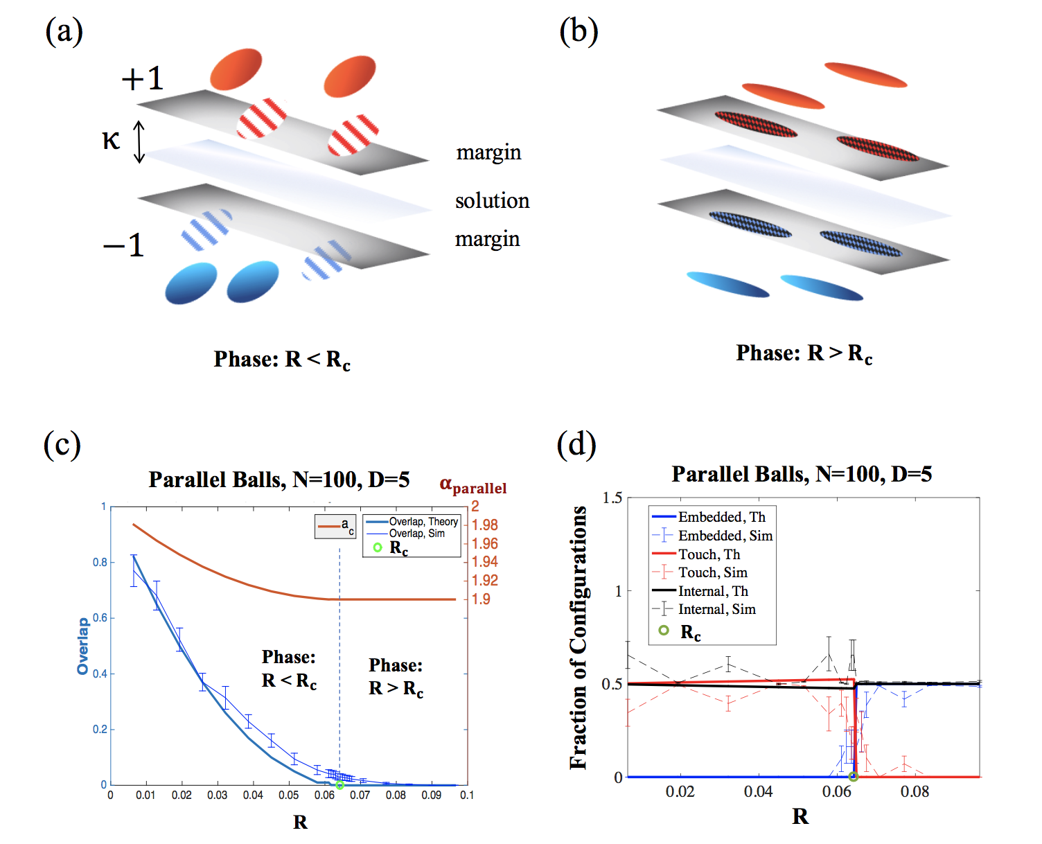
Figure 27: The Phase Transition of Linear Classification of Parallel Manifolds. (a) When $R<R_{c}$ , manifolds are either interior (solid) or touching the margin planes (striped). (b) When $R>R_{c}$ , manifolds are either interior or embedded in the margin planes (diamonds). (c) Phase transition of overlap and capacity at critical radius $R_{c}$, for classification of parallel balls with $D=5$ in ambient dimension $N=100$. The overlap ($\rho$ , Eqn. 286) between the manifold axes and the $\mathbf{w}$ denoting the solution hyperplane vanishes as the ball’s radius $R$ approaches $R_{c}$. The capacity $\alpha_{parallel}$ also goes through phase transition as well, however the value of capacity is stays large, as the embedding dimensions by all manifolds are limited to $D$. (d) Phase transition of manifold configurations at crucial radius $R_{c}$. When $R<R_{c}$ , most manifolds are either interior or touching the margin plane (as shown in (a)), and when $R>R_{c}$ , most manifolds are either embedded or touching the margin plane (as shown in (b)). The simulations and theory show good agreement.

Discussion

We can generalize this analysis to partially parallel correlated balls, where only a fraction of dimensions ($D_{1}=d_{1}N<D$) are shared between them and the rest of the subspaces ($D_{2}=D-D_{1}$) are random. In this case, in the regime where the shared subspaces are orthogonalized, the problem remains as the classification of balls in the null space of the shared subspaces. In this case, the solution will take the form of

$$\alpha_{||}=\alpha_{B}(\kappa_{\rho},R_{\rho},D_{\rho})S_{0}^{-1}(\rho)$$ (295)

where $\alpha_{B}$ is the capacity of balls and $\kappa_{\rho}$ is the effective margin in the null space due to the radii in the parallel subspaces and $R_{\rho}$is the effective radius in the null space due to the random directions and $D_{\rho}$ is the effective ball dimension in the null space due to the random directions. Furthermore, the problem can be generalized to other types of correlations (i.e. correlation between the manifold subspace and the center of the manifold, or the correlation between centers.) We hope to explore these issues of various types of correlations to take into account the structures in the realistic data.

Mixtures of Shapes

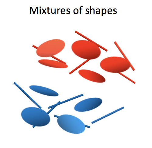
Figure 28: Linear Classification of Mixtures of Shapes (Illustration). The linear classification capacity of mixtures of shapes is given by Eqn. 296.

So far, we have discussed the classification of manifolds with same shapes and sizes. In this section, we generalize the problem to the classification of manifolds with different shapes and sizes. Suppose there are $C$ different manifold types, and each of these types have the capacity of $\alpha_{s}$ where $s=1,...,C$ ($s$ for shape).

In this problem, the self-consistent term $G_{1}$ (the free energy term) is an average of each $G_{1}$ of the classification problem of manifolds of the shape $s$. Recall that $G_{1}$ of each shape determines the capacity for each shape, through $\alpha_{s}^{-1}$.

Then, the linear classification capacity of the mixtures of $C$ different manifold types can be simplified to

$$\alpha_{mixture}^{-1}=\langle\alpha_{s}^{-1}\rangle{}_{s}$$ (296)

where $s=1,...,C$ refers to the index for each manifold type.

This remarkably simple and general theoretical result opens doors to the treatment of a vastly diverse set of manifold classification problems, from classification of manifolds different shapes and sizes to different ratios of labels.

Class Imbalance

So far, we have covered the binary classification of manifolds where the number of positively labeled manifolds is equal to the number of negatively labeled manifolds. Here we consider the class imbalance problem, where the number of positive labels is far less than the number of negative labels, or vice versa. This is also known as classification with sparsity in the labels. In the theory of classification of points, increasing the sparsity of labels has been known to increase the point classification capacity by orders of magnitude (^{gardner1988space}). In this section, we ask the question whether increasing the sparsity of manifold labels also improve the manifold classification capacity.

Note that classification of manifolds with sparse labels is an important example of classification with inhomogeneous manifolds (Section Mixtures of Shapes). Notice that sparsity term $f$ is defined as the fraction of positively (or negatively) labeled manifolds out of the total number of manifolds, so a large sparsity actually refers to a small $f$ (Fig. 29).

One important thing to note is that in the balanced binary classification case where the number of positive and negative labels are equal ($f=0.5$), the bias term, $b$, of the linear classification

$$y^{\mu}\left\{\mathbf{w}^{T}\left(\mathbf{x_{\mathbf{0}}}^{\mu}+\sum_{i=1}^{D}s_{i}\mathbf{u}_{i}^{\mu}\right)+b\right\}\geq\kappa||\mathbf{w}||$$ (297)

was ignored because the optimal bias term which maximizes the classification capacity with balanced labels is $b=0$. However, in the sparse label case, this is no longer true, and the nonzero bias term needs to be included in the evaluation of the capacity, and the bias term needs to be optimized.

Sparse General Manifolds

Using the similar analysis as the calculation of perceptron capacity for mixtures of shapes (Section Mixtures of Shapes), we average the inverse of capacities for the positive and negative labels, and arrive at the expression for the manifold capacity with sparse labels.

Sparse General Manifolds

With this, we can express capacity of general manifolds with label sparsity $f$ as

$$\alpha_{M}^{-1}(\kappa,f)=f\alpha_{M}^{-1}(\kappa+b_{max})+(1-f)\alpha_{M}^{-1}(\kappa-b_{max}).$$ (298)

where

$$b_{max}=\mbox{argmax}_{b}\alpha_{M}(\kappa,f,b)$$

and

$$\alpha_{M}^{-1}(\kappa,f,b)=f\alpha_{M}^{-1}(\kappa+b)+(1-f)\alpha_{M}^{-1}(\kappa-b)$$

Sparse D-dimensional Balls

As an example, we can express capacity of $D$-dimensional $L_{2}$ balls of radius $R$ with label sparsity $f$ as

$$\alpha_{B}^{-1}(\kappa,R,D,f)=f\alpha_{B}^{-1}(\kappa+b_{max},R,D)+(1-f)\alpha_{B}^{-1}(\kappa-b_{max},R,D).$$ (299)

where $b_{max}$ needs to be found so that it maximizes the capacity with sparsity $f$ , i.e.

$$b_{max}=\mbox{argmax}_{b}\alpha_{B}(\kappa,R,D,f,b)$$ (300)

where

$$\alpha_{B}^{-1}(\kappa,R,D,f,b)=f\alpha_{B}^{-1}(\kappa+b,R,D)+(1-f)\alpha_{B}^{-1}(\kappa-b,R,D).$$ (301)

This result implies that similarly to the case of the points, the manifold capacity increases significantly with the increased sparsity (reduced $f$) (Fig. 29).

Fraction of Support Structures

In a similar manner to the replica calculation of fraction of support structures in ^{chung2016linear}, the fraction of support structures for sparse labels can be calculated. Note that due to the asymmetry in the number of positive and negative labels and the non-zero bias, the terms with majority labels and non-majority labels are different. We give here the expression for the fraction of support structures for $D$-dimensional balls. First, manifolds with non-majority labels, which consists of $f$ of the total manifolds can be either embedded, touching, or in the interior side of the shattered space. All together, they consist of the first (non-majority) term of the capacity expression with coefficient $f$, in Eqn. 299.

With this, we can derive the fraction of support structures of manifolds with sparse labels. Unlike the problem with dense labels, the minority manifolds (red manifolds in Fig. 29(a)) and the majority manifolds (blue manifolds in Fig. 29(a)) have different behaviors.

First, fraction of embedded manifolds with non-majority labels is

$$p_{emb}^{minor}=f\int_{0}^{\infty}dt\chi{}_{D}(t)\left[\int_{-\infty}^{\kappa+b-\frac{1}{R}t}Dt_{0}\right]$$ (302)

Then, fraction of manifolds with non-majority labels that touch the margin plane is

$$p_{touch}^{minor}=f\int_{0}^{\infty}dt\chi{}_{D}(t)\left[\int_{\kappa+b-\frac{1}{R}t}^{\kappa+b+Rt}Dt_{0}\right]$$ (303)

The rest of the non-majority manifolds are those in the interior space shattered by the margin planes

$$p_{interior}^{minor}=f\int_{0}^{\infty}dt\chi{}_{D}(t)\left[\int_{\kappa+b+Rt}^{\infty}Dt_{0}\right]$$ (304)

Note that $p_{emb}^{minor}+p_{touch}^{minor}+p_{interior}^{minor}=f$. Similarly, the fraction of embedded manifolds with majority labels is

$$p_{emb}^{major}=(1-f)\int_{0}^{\infty}dt\chi{}_{D}(t)\left[\int_{-\infty}^{\kappa-b-\frac{1}{R}t}Dt_{0}\right]$$ (305)

The fraction of manifolds that touch the margin plane with majority labels is

$$p_{touch}^{major}=(1-f)\int_{0}^{\infty}dt\chi{}_{D}(t)\left[\int_{\kappa-b-\frac{1}{R}t}^{\kappa-b+Rt}Dt_{0}\right]$$ (306)

The fraction of the manifolds with majority labels that are in the interior space shattered by the margin planes is

$$p_{interior}^{major}=(1-f)\int_{0}^{\infty}dt\chi{}_{D}(t)\left[\int_{\kappa-b+Rt}^{\infty}Dt_{0}\right]$$ (307)

Like with the sparse case, Note that $p_{emb}^{major}+p_{touch}^{major}+p_{interior}^{major}=1-f$. The example of this theoretical prediction is tested in Fig. 29(c), where we show that it matches well the fraction of sparse manifold structures in the case of $1D$ manifolds (lines).

Simulations

The linear classification capacity for $2$ dimensional balls with sparsity $f$ has been evaluated numerically and theoretically. For the numerical evaluation, $M_{4}$ algorithm (Chapter The Maximum Margin Manifold Machines) has been used with sparse labels. For the fraction of support structures, $1D$ line manifolds with sparse labels were used. For the theoretical evaluation, the Eqn. 299 and Eqn.302 - 307 has been used, and agree well with the simulations.

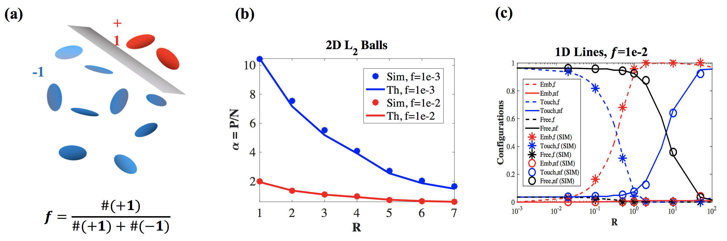
Figure 29: Linear Classification of Balls with Sparse Labels. (a) (Illustration) The solution hyperplane (grey) separates manifolds, where the fraction of positively labeled manifolds out of the total number of manifolds are given by $f\ll 1$ . (b) Capacity of $2D$ $L_{2}$ balls with sparsity $f=0.001$(blue) and $f=0.01$ (red). Theory (line) matches simulations (markers) well. (c) Support configurations of $1D$ line segments with sparsity $f=0.01$, for majority labels (denoted as $nf$, solid line in the legend) and non-majority (sparse) labels (denoted as $f$ , dashed line in the legend). Theory matches simulations well. As $R$ is increased, the fraction of embedded line segments becomes 1, and the transition happens at smaller $R$ in manifolds with non-majority label compared with manifolds with majority labels.

Note that in Fig. 29(c), when $R$ starts out small, most of the non-majority manifolds are touching, and most of the majority manifolds are interior, and as $R$ is increased, the phase transition where most of the sparse manifolds become embedded happens first, and then, the phase transition where most of the non-sparse manifolds become touching happens.

Small $f$ Regime

Let us focus on the $D=1$, the classification of lines with sparsity $f$ . What is the behavior of the line capacity $\alpha_{L}$ , in the case of extreme sparsity, i.e. $f\rightarrow 0$? The dominant term analysis in different regimes of $R$ gives the following analytical approximations for capacity with $\kappa=0$.

1. $R=O(1)$

$$\alpha_{L}^{-1}(R,f)=2(1+R^{2})f|\log f|$$ (308)

2. $f^{-1/2}\gg R\gg 1$

$$\alpha_{L}^{-1}(R,f)=2R^{2}f|\log R^{2}f|$$ (309)

3. $f^{-1}\gg R\gg f^{-1/2}$

$$\alpha_{L}^{-1}(R,f)\approx 1-\frac{2}{\pi R^{2}f}$$ (310)

4. $R\gg f^{-1}$, $R\rightarrow\infty$

$$\alpha_{L}^{-1}(R,f)=1+2f|\log f|$$ (311)

It is interesting to note that in the limit of large $R,$ the capacity does not depend on the $R$ any more.

Object Recognition Limit, $f=1/P$

Particularly interesting regime is when the sparsity $f$ is equivalent to $1/P$ where $P$ is number of manifolds. This is analogous to the one-vs-all task in the multi-class classification problem, where the output unit is activated only when the input comes from the correct class out of the possible $P$ classes. Can we estimate the capacity of object manifolds, in this relevant sparse object recognition limit?

Using our theory, the minimum network size $N^{*}$required in order to classify one manifold out of $P$ given manifolds can be estimated to be

$$N^{*}=P/\alpha_{M}\left(f=\frac{1}{P}\right)$$ (312)

where we can use $1/P$ as sparsity $f$ .

One can also estimate the largest allowed size of the manifolds if one is given with the network size $N$ and the number of object manifolds $P$. That is, solve for $R$ and $D$ such that

$$\frac{P}{N}=\alpha_{\text{B}}(\kappa,R,D,\frac{1}{P})$$ (313)

which can be found numerically.

Simulation Results and Discussion

We tested below the capacity of line segments, in the one-vs-all object recognition task limit. In the simulations where critical $P^{*}$(number of classes/manifolds) had to be found, we fixed the network size, $N=100$ and $N=200$, and $P$ was varied to find $P^{*}$ at which the probability of finding a linear classifier goes from 1 to 0, given 100 repetitions. The theoretical prediction matches the simulation capacity well (Fig. 30(a)).

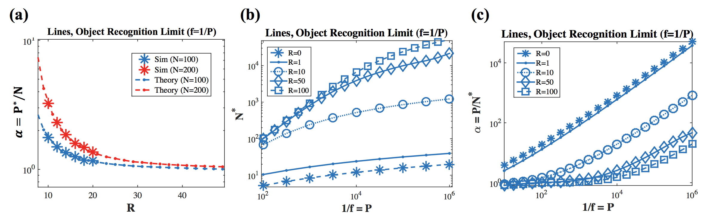
Figure 30: Line Classification of Line Segments in Object Recognition Limit ($f=1/P$). (a) Capacity $(\alpha_{L}(f=1/P))$ as a function of size $R$ for different network sizes. (b) Minimum network size required for linear separability ($N^{*}$) as a function of number of manifolds/objects ($P$), for different sizes $R$ (c) Capacity as a function of number of manifolds/objects ($P$).

If we want to classify $P=1000$ classes, whose object manifolds are 1 dimensional, with one-versus-all task, how many neurons are required for the problem to be linearly separable? Figure 30(b) provides an answer to that question with our theoretical estimate of minimum required network size $N^{*}$. In the limit of point, $R=0$, roughly $N^{*}=10$ is enough to classify 1000 objects. However, if $R>50$, at least $N^{*}=1000$ is required to be linearly separable.

Notice that the capacity in the units of load $(P/N)$ shows an interesting behavior in the limit of large $R$ in Figure 30(c). Notice that in large $R$ , the capacity is dominated by $1/D$ and the improvement due to sparsity is smaller than when $R$ is small. In other words, if the manifold sizes are large, making the labels sparse does not improve the capacity as much as when the manifold sizes are small. Therefore, the effect of size of the manifold $(R)$ on the capacity is more dramatic in the case of classification with sparsity in the object recognition limit (compared to the dense label classification).

Building Multi Layer Networks of Sparse Classifiers

In the section Class Imbalance, we showed how introducing the sparsity in the manifold labels improves substantially the classification capacity of manifolds. Here we show that we can use this feature to solve dense classification task. The general idea is as follows. Suppose we have an input neural layer with size $N$ representing $P$ manifolds and a dense classification task (i.e. label sparsity $f$ is $\sim 0.5$), such that a linear classifier applied directly to this input layer fails to classify all stimuli correctly, namely, the manifolds in the input representations are not linearly separable.

To solve the task we add a single hidden layer with $M$ binary units (Fig. 31(a)). We would like to generate a hidden layer representation of the manifolds that is invariant, namely that all inputs from a given manifold are mapped to a single activity pattern in the hidden layer. If we can achieve this, the invariant representations in the hidden layer can easily be linearly separable. In order to generate this invariant representations in the intermediate layer, we generate $M$ random sparse labels for each manifold, and learn the connection from the input layer to the intermediate layer as a sparse linear classification in each unit in the intermediate layer, which we assume is below the capacity and therefore can be implemented without error. In the following subsection below, we analyze the range of parameters and the performance of this two layer network.

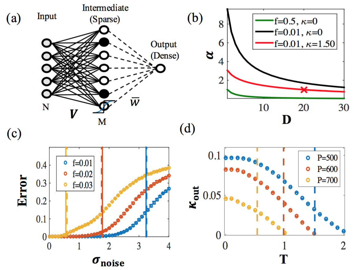
Figure 31: Sparse Intermediate Representation Enhances the Invariant Processing of Manifolds. (a) Input layer with dimension $N$, where input vectors are drawn from a set of $P$ manifolds. The weight matrix, $\boldsymbol{V}$, from the input to the intermediate layer is constructed so that each node in the intermediate layer is activated in invariant manner by randomly chosen fP manifolds (where $f$ is sparsity). This yields a sparse representation where all inputs from the same manifold activates the same fM intermediate nodes. Output node classifies the manifolds with desired dense binary labels. (b) Perceptron capacity of manifold classification, $\alpha=P/N$ versus manifold ball dimension $D$ at $R=1$, for different sparsity ($f$) and margin ($\kappa$). The X marker denotes the working point for simulation in (c-d). (c-d): Robustness to noise. (c) Probability of error at output layer, versus the standard deviation of the input additive Gaussian noise $(\sigma_{\mbox{noise}})$ for different intermediate layer sparsity $f$. Input manifold dimension and radius are: $D=20$ and $R=1$. For simulation, $N=M=500$, and number of manifolds $P=250$ (which is five times the single layer capacity, $P_{\mbox{SL}}=\alpha_{\mbox{SL}}N\approx 48$, for $\kappa=0$, for these manifolds). Markers indicate the simulation results for the error for different sparsities. Robustness to noise is achieved by ensuring a significant margin $\kappa_{\mbox{int}}$ at the intermediate nodes; the margins $\kappa_{\mbox{int}}$ are shown as vertical lines. (dashed) simulation (solid) analytical prediction. Higher sparsity ($f=0.01)$ ensures larger margin, and more robustness to input layer variability. (d) Output margin ($\kappa_{\mbox{out}}$) versus the smoothness parameter ($T$) of the sigmoid in the intermediate layer $(1+e^{-x/T})^{-1}$, for different number of manifolds, $P$. $T=0$ is the binary limit. For the simulation, $N=500$, $M=500$, $f=0.01$, $R=1$, $D=20$ was used. Values of $P$ are an order of magnitude larger than the single layer capacity of the input layer which is $P_{\mbox{SL}}\approx 48$. (vertical lines) intermediate layer margins. For the same $f$, smaller number of manifolds ($P=500$) allows larger margin, and higher robustness to the smoothing of the intermediate layer responses and the resultant manifold variability.

Capacity of Two-Layer Network with Sparse Invariant Representation

As a simple example, we focus on input manifolds of $D$ dimensional balls with radius $R$ such that $P$ (number of balls) is larger than the linear classification capacity of such balls, $N\alpha_{B}(R,D)$. We first compute the perceptron capacity for manifolds with sparse labels, parametrized as above by $\kappa$ $D$, $R$ and $f$ , $\alpha_{B}(\kappa,R,D,f)$ , where $f$ is the fraction of positive examples. Similar to classification of points^{gardner1988space, babadi2014sparseness}, the perceptron capacity of manifolds with sparse $f\ll 1,$ is much higher than when the labels are dense ($f=0.5)$ (Fig. 31(a)). Consider now the task of invariant classification of manifolds where the task labels are dense, (e.g., $f=0.5,$ and $\kappa=0$). If the number of manifolds $P$ relative to the size of the input layer, $N$ is above $\alpha_{B}(\kappa,R,D,0.5$), then the single layer architecture will be unable to solve the linear classification task. However, we can use the improved perceptron capacity for sparse labels (Fig. 31(b)), to construct an intermediate representation of $M$ nodes, each one of them trained for a randomly chosen sparse labeling of the manifolds. These sparse labels are unrelated to the task labels; they are used solely for building the intermediate representation. As long as $P/N$ is below the perceptron capacity for sparse classification of manifolds, the resultant intermediate layer generates an invariant representation. The subsequent single layer readout at the output layer can then perform the required dense classification as long as $P/M<\alpha_{0}(\kappa,f=0.5)$, namely the perceptron capacity for dense labels of points. The overall capacity for classification of manifolds of this two-layer network is given by $\alpha_{B}^{TL}(0,R,f=0.5)=\mbox{min}\left(2M,\>N\alpha_{D}(0,R,f)\right)/N$, where $TL$ stands for two layer, much higher than that of the single layer ($SL$), $\alpha_{\mbox{SL}}=\alpha_{B}(0,R,D,0.5)$ (for $M\geq N$) (Fig. 31(c-d) captions). In addition, below the zero-margin capacity, $\alpha_{\mbox{D}}^{TL}(0,R,f=0.5)$, the maximum margin $\kappa_{\mbox{out}}$ at the output node is given by $\alpha_{0}(\kappa_{\mbox{out}},0.5)=P/M$.

Robustness to Noise

This two-layer architecture shows not only enhanced capacity, but can also enhance the system’s robustness to noise. To achieve robustness, the sparsity of the intermediate representation should be sufficiently large to have a significant margin, $\kappa_{\mbox{int}}>0$ in their representation (where subscript ’int’ stands for intermediate layer), i.e, $P/N<\alpha_{D}(\kappa_{\mbox{int}},R,f)$. Then adding noise may cause the sparse representation in the intermediate layer to be only approximately invariant to the input manifold degrees of freedom, nevertheless the effect on the performance will be small provided the noise level is small compared with $\kappa_{\mbox{int}}$. We demonstrate this in two cases. First, additive full-rank Gaussian noise was introduced to the input layer. As shown in (Fig. 31(c)) the two layer network is robust to a range of noise values, and networks with sparser intermediate representations have output error probabilities close to zero for a larger range of noise. For output noise in the intermediate layer we haven’t analyzed the performance explicitly, but we present the heuristic analysis based on the idea that the level of robustness to noise in each unit should be determined by the size of each intermediate unit’s classification margin $\kappa_{\text{int}}$. The details of the numerics are given in the appendix to the chapter (Section Multi-Layer Networks with Sparse Intermediate Layer).

Next, stochasticity in the activation of the intermediate binary units is modeled by changing their activation function to smooth sigmoidal units with gain parameter $1/T$. Smooth rate functions are also more representative of biologically realistic rate-based models of neural networks. Fig. 31(d) shows that for a broad range of $T$ the output readout was able to correctly classify the manifolds. The critical value of $T$ above which classification fails is roughly given by the margin of the intermediate layer. These examples show how to construct a network able to classify manifolds with small error even when the intermediate layer is not completely invariant to the manifold representation.

Discussion

In this section, we have shown that by using classifiers of manifolds with sparse labels, a two layer network can be constructed with enhanced manifold processing capacity and robustness to noise. Thus, our theory provides a biologically plausible simple feedforward network model that is capable of processing object relation information in an invariant manner. The current theory can be extended to in several important ways. Here we focused on training the network weights with full manifolds and adding an additive noise after training, but the network weights can be trained with subsamples of manifolds, or with noisy realizations of manifolds. Here we focused on the intermediate layer nonlinearity to be a sigmoid function, but other types of nonlinearities such as ReLu can be considered, which can have a different effect on the reformatted shape of the manifold. Intermediate layer invariance can be achieved by different methods such as max-pooling or polynomial nonlinearities, and we hope to explore the role of such processing on the reformatting of the manifolds using the manifold capacity framework in the future.

Kernel Extensions

In section Building Multi Layer Networks of Sparse Classifiers, we showed how an additional intermediate layer with sparsity can improve the output readout capacity for manifolds. This is an example where a nonlinearity in each unit in the intermediate layer created a new representation that is easier to be read out by the output unit. In this section, we show another example of how nonlinear processing reformats the input manifolds so that the output linear separability is improved, by using kernels.

Traditionally, nonlinear kernels have been used in the SVM dual framework to allow for nonlinear classification of points ^{vapnik1998statistical}. Here we show that when input patterns are on manifolds, how nonlinear kernels achieve the non-linear classification can be analyzed as improved manifold classification capacity of reformatted manifolds in the kernel feature space (Fig. 32^{burges1999geometry}). We also extend $M^{4}$ algorithm provided in Chapter The Maximum Margin Manifold Machines to show that an iterative method with the same principle can be used to find a kernel-SVM solution for manifold classification (kernel-$M^{4}$).

Manifold Capacity under a Quadratic Kernel

The effect of the kernel operation on the geometric properties of the manifolds depends on the kernels. As a simple example of a non-linear kernel, we study the improved classification capacity of manifolds with quadratic kernels. We extend our theory to provide upper and lower bounds for the classification capacity of manifolds with dimensionality $D$ in input space after their transformation to a quadratic feature space.

Consider arbitrary manifolds embedded in $D$-dimension, where each point in the manifold can be expressed as $\mathbf{x}=\mathbf{x}_{0}+\sum_{i=1}^{D}s_{i}\mathbf{u}^{i}$, where $\mathbf{x}_{0}$ is a $N$-dimensional center vector and $\mathbf{u}^{i}$ ($i=1,...,D$) are the basis vectors, and parametrized by $\vec{s}$, where $s_{i}$ corresponds to the $i$ th basis vector. The feature space of a homogenous quadratic kernel is $\left\{x_{i}x_{j},i\leq j\right\}$ which has $N_{f}=(N+1)N/2$ unique components. The feature space, $\left(\mathbf{x}_{0}+\sum_{k=1}^{D}s_{k}\mathbf{u}^{k}\right)_{i}\left(\mathbf{x}_{0}+\sum_{l=1}^{D}s_{l}\mathbf{u}^{l}\right)_{j}$, can be expanded as $x_{0i}x_{0j}+\sum_{k}s_{k}\left(u_{i}^{k}x_{0j}+x_{0i}u_{j}^{k}\right)+\sum_{k=1}^{D}\sum_{l=1}^{D}s_{k}s_{l}u_{i}^{k}u_{j}^{l}$. This is $N_{f}$-dimensional vector with a center $x_{0i}x_{0j}$ and $(D+3)D/2$ basis vectors. The basis vectors consist of the two classes: $u^{k}u^{l}$ where there are $(D+1)D/2$ of them, and $\left(u_{i}^{k}x_{0j}+x_{0i}u_{j}^{k}\right)$ where there are $D$ of them. Therefore, for input space dimension $N$, the ambient dimension in this feature space is $N_{f}=(N+1)N/2$. On the other hand, the dimensionality of the manifolds in feature space is $D(D+3)/2$.

In order to illustrate the effect of kernels on the learning of classifier of the manifolds, we present 2 simple examples. Quadratic kernels applied to $1D$ lines and $2D$ circles. The geometric illustration of how$1D$ lines and $2D$ circles with radius $R$ map from input space to quadratic kernel’s feature space is provided in Fig. 32(a),(c). For $R=0$, the (zero margin) capacity $P$ increases from $2N$ to $(N+1)N$, as given by the capacity for classifying points. On the other hand, for $R=\infty$, the weight vector has to be orthogonal to all the dimensions spanned by the reformatted manifolds, yielding the capacity $P=\frac{N(N+1)}{(1+D(D+3))}$ in this limit. For an intermediate $R$, the capacity will be affected by the extent and geometry of the manifolds in feature space. The predicted bounds are compared with numerical simulations in Fig. 32. These considerations can be easily generalized to polynomial kernels with higher degree.

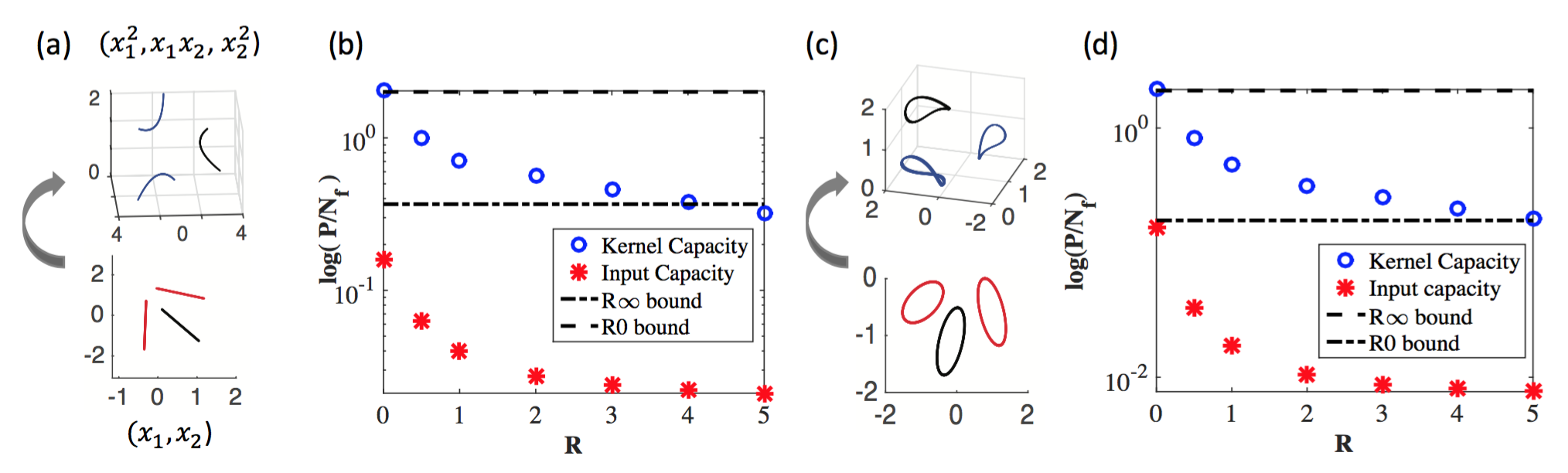
Figure 32: Manifold Classification with a Quadratic Kernel. (a) Classification of Lines embedded in $N$-dim input space (black versus red, bottom) maps to $2D$ curves (black vs. blue, top) embedded in $N_{f}=(N+1)N/2$ dim kernel feature space. (b) Line capacity in input space (red), and quadratic kernel space (blue), shown as $P$ (number of manifolds) over $N_{f}$, and the bounds on the kernel capacity: $\alpha=2$ ($R=0$) and $\alpha=2/5$($R=\infty,D=2$) (dashed lines). (c) Classification of $2D$ circles (black v. red, bottom) maps to $5D$ manifolds (black vs. blue, top). (d) Manifold capacity of $2D$ circles in input space (red) and quadratic kernel space (blue), and the bounds on the kernel capacity: $\alpha=2$ ($R=0$) and $\alpha=2/11$($R=\infty,D=5$). In both the line and 2D circles, the manifold capacities are improved by the quadratic kernel operation.

Kernel-$M^{4}$ Algorithm

General Framework

The Kernel-$M^{4}$ algorithm applies the same logic as the $M^{4}$ algorithm in the chapter The Maximum Margin Manifold Machines, but in the dual SVM framework. The separating hyperplane is represented implicitly by dual coefficients $\vec{\alpha}$ and point examples $\left(\mathbf{x}_{l},y_{l}\right)$ and a bias $b$, and the field induced by an input $\mathbf{x}$ is given as $\sum_{l}\alpha_{l}y_{l}K\left(\mathbf{x},\mathbf{x}_{l}\right)+b$. The Kernel-$M^{4}$ algorithm iteratively calls a quadratic optimization solver on a finite number of labeled examples in the dual framework. Given a current estimate of $\vec{\alpha}$ and $b$ , the algorithm searches for the point on the manifolds with the worst margin. If the margin of the new point is worse than the previous estimate, the point set is augmented, i.e. the kernel matrix is increased by one column and row, and the dual SVM solver is run to update values for $\vec{\alpha}$ and $b$. The pseudocode for kernel-$M^{4}$is given by Alg. 7.

[$\vec{\alpha}$,$b$] = function kernel-M4($K$ , $S$ ,$\epsilon$ )

Input: kernel type $K$ , data manifold parameters $S$ , tolerance $\epsilon$

Initialize: $\vec{\alpha}$,$b$, $\delta$

$t=0$

while $\delta>\epsilon$ do

   1. $t=t+1$

   2.$\alpha^{t}=$ $\max_{\alpha_{l}\geq 0}\sum_{l=1}^{M}\alpha_{l}-\frac{1}{2}\sum_{j=1}^{M}\sum_{k=1}^{M}\alpha_{j}\alpha_{k}y_{j}y_{k}K\left(\mathbf{x}_{j},\mathbf{x}_{k}\right)$ for $\forall\nu<t$ and and $\alpha^{tT}y=0$.

   3. Compute $b$ and $h_{min}^{t}$.

   4. Search for the new pattern such that $\frac{\left(h_{min}^{t}\right)_{new}}{||w||}=\left\{\mbox{min}_{\vec{s},\mu}y_{\mu}\left(\sum_{l}\alpha_{l}y_{l}K\left(\mathbf{x}_{l},\mathbf{x}_{\mu}(\vec{s})\right)+b\right)\right\}$.

   5. $\delta=\left\|\left(h_{min}^{t}\right)_{new}-h_{min}^{t}\right\|$

end

Output: $\alpha$, $b$

Algorithm 7 Pseudocode for kernel-$M^{4}$

In general, finding the point with the worst margin in the kernel feature space may be hard as the convexity of the input manifolds may be lost by the nonlinear kernel operation. If the manifolds are given by finite sets of points, then, the search over all points to find the worst point can be performed, where each search is upper bounded by the number of examples. If the input manifolds are uncountable sets of points, where the complete parameterization for the shape $f(\vec{s})=0$ is given, then the search for the worst point is limited to finding the worst $\vec{s}^{*}$, and sometimes $\vec{s}^{*}$ may be found analytically. If the parameterization is not available, then one may need to find the worst point with a local search using a gradient, but if there is no estimate of the convex hull, this operation is not necessarily a convex problem, which may be investigated further in the future.

With certain manifolds and kernel functions, the worst point operation can still be done efficiently. As an illustrative example, we demonstrate an example of the maximum margin classification of line segments and $2D$ circles under a homogenous quadratic kernel, $K\left(\mathbf{x}_{j},\mathbf{x}_{k}\right)=\left(\mathbf{x}_{j}^{T}\mathbf{x}_{k}\right)^{2}$. For these examples, we can reduce the worst point operation to a finite set of analytical solutions, which is as efficient as regular$M^{4}$operation. This computation can also be generalized to $D$-dimensional balls.

$D$-dimensional Balls and Quadratic Kernel $M^{4}$

Here we show an example of quadratic kernel-$M^{4}$with $D$-dimensional balls with radius $R$. In this case, finding the smallest distance to the solution plane from each point on the manifold in the kernel space is:

$$\underset{\mbox{$\vec{s}$},f_{\mu}(\vec{s})=0}{\text{argmin}}h^{*}(\vec{s})=\underset{\mbox{$\vec{s}$},f_{\mu}(\vec{s})=0}{\text{argmin}}y_{\mu}\left(\sum_{j=1}^{M}\alpha_{j}y_{j}K\left(\mathbf{x}_{j},\mathbf{x}(\vec{s})\right)+b\right)$$ (314)

where $\mathbf{x}=\mathbf{x}_{0}^{\mu}+\sum_{i=1}^{D}s_{i}\mathbf{u}_{i}^{\mu}$, and $f_{\mu}(\vec{s})=0$ is the shape constraint of the $\mu$th ball.

Now, the closet point in the $D$-dimensional ball manifold $\mu$ can be found by considering

$$\vec{s}^{*}=\mbox{argmin}_{\vec{s}}\left[y_{\mu}\left(\sum_{l=1}^{\nu}\alpha_{l}y_{l}K\left(\mathbf{x_{l}},\mathbf{x}_{0}^{\mu}+R\sum_{j=1}^{D}s_{j}\mathbf{u}_{j}^{\mu}\right)+b\right)+\lambda\left\{\sum_{j=1}^{D}s_{j}^{2}-1\right\}\right]$$ (315)

This is in general hard, but analytically solvable for quadratic kernel and a ball. For a homogenous quadratic kernel $K(\mathbf{x}_{n},\mathbf{x}_{m})=\left(\mathbf{x}_{n}^{T}\mathbf{x}_{m}\right)^{2}$, we solve for $\vec{s}^{*}$ by taking a derivative of $h(\vec{s})$.

The worst point $\vec{s}^{*}$ on the $\mu$th $D$-dimensional balls are found to be

$$\lambda\left\{s_{j}^{\mu}\right\}^{*}=A_{j}^{\mu}+\sum_{j^{\prime}=1}^{D}B_{jj^{\prime}}^{\mu}s_{j^{\prime}}^{\mu k}$$

where

$$A_{j}^{\mu}=y_{\mu}\sum_{l=1}^{\nu}\alpha_{l}y_{l}\left[\left\{\mathbf{x}_{l}^{T}\mathbf{x}_{0}^{\mu}\right\}\left(\mathbf{x}_{l}^{T}\mathbf{u}_{j}^{\mu}\right)\right]$$

$$B_{jj^{\prime}}^{\mu}=Ry_{\mu}\left[\sum_{l=1}^{\nu}\alpha_{l}y_{l}\left(\mathbf{x}_{l}^{T}\mathbf{u}_{j}^{\mu}\right)\left(\mathbf{x}_{l}^{T}\mathbf{u}_{j^{\prime}}^{\mu}\right)\right]$$

with normalization on $\left\|\vec{s}^{*}\right\|=1$, and $j,j^{\prime}=\{1,...,D\}$, and $\vec{\alpha}$ , $\vec{y}$ are given. $l=1,...,\nu$ is an index of all the training points added so far,

And for line segments, the worst point $s^{*}$ on the $\mu$ th line is

$$a^{\mu}+b^{\mu}\left(s^{\mu}\right)^{*}=\lambda\left(s^{\mu}\right)^{*}$$

where

$$a=y_{\mu}\sum_{l=1}^{\nu}\alpha_{l}y_{l}\left[\left\{\mathbf{x}_{l}^{T}\mathbf{x}_{0}^{\mu}\right\}\left(\mathbf{x}_{l}^{T}\mathbf{u}^{\mu}\right)\right]$$

$$b=Ry_{\mu}\left[\sum_{l=1}^{\nu}\alpha_{l}y_{l}\left(\mathbf{x}_{l}^{T}\mathbf{u}^{\mu}\right)\left(\mathbf{x}_{l}^{T}\mathbf{u}^{\mu}\right)\right]$$

with normalization on $\left\|\vec{s}^{*}\right\|=1$.

In general, the solution for $\vec{s}^{*}$ has two classes. One is where the closest point to the hyperplane in the kernel space comes from the interior area of the convex hulls of the manifold in the input space ($\lambda=0$ ), and the other is when $\vec{s}^{*}$ comes from the convex hull in the input space (nonzero $\lambda$). Generally, one can solve for both cases, and check which $\vec{s}^{*}$ gives a smaller field, by computing Eqn. 314 for each $\mu$ and do this over all manifolds, and with $P$ candidate points, find the smallest one again. This is the step 4 of Alg. 7, for $D$-dimensional balls.

Discussion

In this section, we showed how the role of nonlinear kernel on data manifolds with small manifold capacity (in other words, linearly non-separable manifolds) in the input layer can be viewed as reformatting them to increase the manifolds capacity in the nonlinear feature space, using quadratic kernels and simple $1D$ and $2D$ balls in the input space as examples. Which kernels are best suited for the classification problem depends on the types of the data, which, in our case, are manifold structures. We laid the ground here for future analysis with manifolds capacity in kernel feature space, by formulating the iterative algorithm for finding the max margin solution for manifolds with kernels and demonstrating the simple examples of $1D$ and $2D$ balls, as well as providing bounds on their manifold capacities in input and feature space. Enabled with our theory of capacity of general manifolds (Chapter Linear Classification of General Manifolds), we hope to extend our manifold capacity analysis for more complex manifolds to study the role of nonlinear kernels.

Generalization Error

So far, we have considered different aspects and extensions of manifold classification capacity, mainly motivated by a linear classifier that achieves zero training error. However, another important aspect of the linear separability of data manifolds is the generalization error of a linear classifier. This is particularly relevant in more realistic settings, where the manifolds given for training are not full manifolds, but only a subset of the manifolds. An example of this would be when the training data are convex hulls of subsamples of underlying manifolds. Another relevant case is when there is noise in the input. By focusing on the distribution of fields arising from manifold structures, here we show how the our theory allows for the estimation of generalization error for the manifold classification problem.

Generalization Error for General Manifolds, Given Weights.

Exact analytical expression for the generalization error for general manifolds is complicated; furthermore, the error depends on the assumed sampling measure on the manifold (whereas the separability problem is measure invariant). However, in the case of linearly separable manifolds with high $D$ we can use the insight from the above theory (the notions of effective dimensions and radii) to derive a particularly simple approximation.

Assume we have obtained a set of weights from learning manifolds either from subsampling or from full unrealizable manifolds, so that we have a vector $\mathbf{w}$ . Then, the generalization error can be expressed as

$$\epsilon_{G}^{\mu}=\left\langle\Theta\left(-h_{0}^{\mu}-\sum_{i}s_{i}h_{i}^{\mu}\right)\right\rangle_{s}$$ (316)

where $h_{0}$are the field on the center $\mathbf{x}_{0}$and $h_{i}$are the $D$ fields on the basis vector$\mathbf{u}_{i}$, generated by the trained $\mathbf{w}$. The average over $\vec{s}$ is an integration with constraint $f(\vec{s})=0$ . In other words,

$$\langle F(\vec{s})\rangle_{\vec{s}}=\int d\vec{s}p(\vec{s})\delta(f(\vec{s}))F(\vec{s})$$ (317)

and we assume $\int d\vec{s}p(\vec{s})\delta(f(\vec{s}))$=1 . An important point to note is that the generalization error is in general sensitive to the choice of measure to use in this average i.e., $p(\vec{s})$ .

The dependence on the weight $\mathbf{w}$ is via the fields $h_{0}$ and $\vec{h}$. Depending on the learning rule used to generate $\mathbf{w}$, the above fields induced by $\mathbf{w}$ in general will not be the same for all manifolds but will vary with a distribution $P(h_{0},\vec{h})$ even if all manifolds have the same geometry. For example if $\mathbf{w}$ is trained by the max margin classification of subsampled manifolds, $P(h_{0})$ will be the distribution described in Chapter Linear Classification of General Manifolds for finite point manifolds. Therefore, for a given $\mathbf{w}$, the generalization error can be expressed as a double averaging

$$\epsilon_{G}=\left\langle\left\langle\Theta\left(-h_{0}-\sum_{i}s_{i}h_{i}\right)\right\rangle_{\vec{s}}\right\rangle_{h_{0},h_{i}}$$ (318)

Gaussian Approximation in High Dimensional Manifolds.

In high dimensional manifolds, we assume that $h_{i}$ are distributed as projections of gaussian $\mathbf{w}$ on the $\mathbf{u}_{i}^{\prime}s$ . Hence $h_{i}$ themselves are i.i.d. Gaussian distributed with norm $1$. If we make this assumption we get,

$$\epsilon_{G}^{\mu}=\left\langle\left\langle\Theta\left(-h_{0}^{\mu}-z\right)\right\rangle_{z}\right\rangle_{s}$$ (319)

In other words,

$$\epsilon_{G}=\left\langle H\left(\frac{h_{0}}{\sigma}\right)\right\rangle_{h_{0}}$$ (320)

where the width of the distribution is roughly

$$\sigma^{2}\approx\langle\vec{s}\cdot\vec{s}\rangle\approx R_{W}^{2}$$ (321)

in the crude approximation.

We might want to take into account the fact that the $h_{i}^{\prime}s$ are bounded so they are not unbounded Gaussians. We can use the mean width of the manifold $R_{W}\sqrt{D_{W}}$ (Fig. 33(a)) as a measure of the bound. Finally, we can estimate the generalization error to be

$$\epsilon_{G}=\left\langle\frac{H(\frac{h_{0}(w)}{R_{W}})-H\left(\sqrt{D_{W}}\right)}{1-2H\left(\sqrt{D_{W}}\right)}\right\rangle_{h_{0}}$$ (322)

where we added a normalization so that $\epsilon_{G}=0.5$ for $h_{0}=0$. Note that $h_{0}$ is the field from the center, and $D_{W}$ and $R_{W}$ are effective dimension and effective radius of a manifold identified in Chapter Linear Classification of General Manifolds. Intuitively, the generalization error shows the fraction of a manifold on the wrong side of the hyperplane, which is approximated by the area under one end of the tail of a Gaussian distribution outside of the size of the center field induced by the solution $\mathbf{w}$, divided by the area under the Gaussian distribution with tails cut at the size of the mean width from both end (approximately 1 in high $D_{W}$ regime). This relation is shown in the Figure 33.

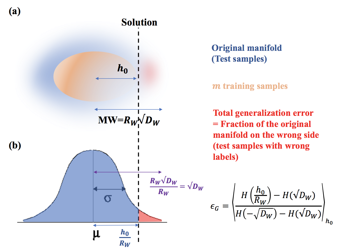
Figure 33: Generalization Error from Each Manifold. (a) The solution hyperplane (dashed line) is determined by the training samples given by the manifold (Orange manifold), and the distance between the center of the original manifold (assuming the center of the testing manifold and original manifold is the same) and the solution hyperplane is given by $h_{0}$ (along the direction of $\mathbf{w}$ ), the field induced by the testing manifold center. The size of the original (testing) manifold, along the direction of $\mathbf{w}$ , is approximated by the Mean Width, $R_{W}\sqrt{D_{W}}$ . (b) The generalization error is the fraction of samples on the correct side of the hyperplane out of the total samples (which is measure-dependent). Assuming the projections of the manifold along $\mathbf{w}$ are Gaussian, we approximate generalization error as ratio between the blue area and blue plus red area under the gaussian. The width of the gaussian is estimated to be $\sigma=R_{W}$ as a crude approximation (assuming $h_{i}$’s are Gaussians with norm 1), with the tails truncated at$R_{W}\sqrt{D_{W}}$, and the distance between the peak and the location of the hyperplane at $h_{0}$ (the separation between correct and incorrect labels). Rescaling the $x$ axis such that $\sigma$ is 1, we get the expression $\epsilon_{G}\sim\langle\frac{H(\frac{h_{0}}{R_{W}})-H(\sqrt{D_{W}})}{H(-\sqrt{D_{W}})-H(\sqrt{D_{W}})}\rangle$.

The generalization error shows two regimes. In the case where full (underlying) manifolds are linearly separable with margin $\kappa$, Then the generalization error will eventually vanish as more samples per manifold , $m$ , are presented during the training.

One thing to note is that as we increase the number of subsamples for training $m$, the size of $h_{0}$ must grow, as the hyperplane is always outside the mean width of the subsampled manifolds. According to the extreme value theory, we expect the max distance between the manifold center and extreme tail to grow like $\sqrt{2\text{log}m}$, like the $m$th maximum value of samples of Gaussian iid distribution ^{bovier2005extreme}. In the limit of large $m$ , we obtain,

$$\epsilon_{g}(m)\sim H(\kappa(m)+\sqrt{2\text{log}m})\propto\frac{\exp[-\kappa\sqrt{2\log m}]}{m}$$ (323)

Interestingly, this decay is faster than the generic power law, $\epsilon_{g}(m)\propto m^{-1}$ of generalization bounds in linearly separable problem and reflects the presence of finite margin of the entire manifold. This dependence is demonstrated in Figure 34 (a1-a2) using ellipsoids.

In the case where the full manifolds are not separable and $\alpha$ is above the capacity, even subsampled manifolds with $m$ points are not necessarily separable. Because the solution hyperplane may intersect the sampled manifolds, $h_{0}$ no longer scales like $\sqrt{2\text{log}m}$. Perhaps for this reason, the $m$ dependence of generalization error given inseparable underlying manifolds is more like conventional general power law, $\epsilon_{g}(m)-\epsilon_{g}(m=\infty)\propto m^{-1}$. This is shown in 34 (b1-b2) using ellipsoids.

Numerical Investigations

As a simple example, we computed the generalization error for a binary dense classification of $P$ ellipsoids, where $R_{i}$ (radius in $i$ th embedding dimension) is sampled from an uniform distribution of $Unif[0.5R_{0},1.5R_{0}]$, and centers and axes are random Gaussian distribution. From each ellipsoid, $m$ training samples and $m_{g}$ test samples were sampled, so that $s_{i}R_{i}^{-1}$ is from a uniform spherical distribution. With these $mP$ finite training samples, max margin solution was found using a standard slack-SVM solver, and generalization error was computed using $m_{g}P$ test samples. Using the centers of the ellipsoids and the max margin solution $\mathbf{w}$, theoretical estimation of the generalization error was computed using Eqn. 322. We show the results of this simulation in Fig. 34.

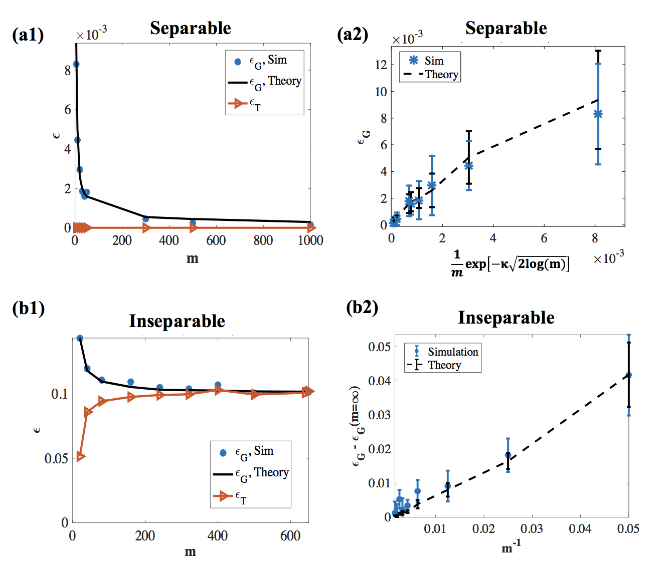
Figure 34: Generalization Error of Ellipsoids Classification as a Function of Number of Subsamples Per Manifold ($m$ ). (a1-a2) In the regime where the full manifolds are separable, the generalization error approaches zero as $m$ is increased, at the rate of $\epsilon_{G}\sim\frac{1}{m}\text{exp}[-\kappa\sqrt{2\text{log}m}]$. The manifolds used were $D$-dimensional ellipsoids with $R_{i}\sim Unif[0.5R_{0},1.5R_{0}]$ and $P=10,N=50,R_{0}=1.00,D=50$. (b1-b2) In the regime where the full manifolds are not separable, the generalization error approaches at the rate of $\epsilon_{G}-\epsilon_{G}(m=\infty)\sim m^{-1}$ . The parameters for the ellipsoids used for the simulation were $P=20,N=50,R_{0}=2.00,D=50$. In all simulations generalization error was tested with $m_{g}=1000$ per manifold. The theoretical predictions for generalization error patches the generalization error calculated by the simulation well in this regime.

We find that the Gaussian approximation of the generalization error works quite well, and the estimation matches the generalization error using simulations. We find that indeed in the separable case, the $\epsilon_{G}$ is close to $\frac{1}{m}exp[-\kappa\sqrt{2logm}]$, and in the inseparable case, $\epsilon_{g}(m)-\epsilon_{g}(m=\infty)$ is approximately $1/m.$

Discussion

Here we demonstrated how the insights from the manifolds capacity theory can be used to compute the crude approximation of generalization error in the high embedding dimension, which works surprisingly well in the case of classification of ellipsoids. Clearly, we made some assumptions for the sake of the approximation (i.e. $h_{i}$ are Gaussians). The fully general replica theory of generalization error for manifolds will require considerations of the actual manifold geometry, and the measure of the samples on the manifold, $p(\vec{s})$, and using the manifold-dependent distribution of fields $h_{0}$ and $h_{i}$ from the replica theory.

Analysis of GoogLeNet Manifolds

So far, we have considered various extensions of the theory of manifold classification for the analysis and application to real data. In this section, we show how our manifold capacity theory can be applied to realistic data, by analyzing manifold representations in conventional deep networks as an illustrative example. In the recent years, the performance of the artificial systems for visual classification tasks has been focused on the generalization error of the final layer on the test dataset. However, the underlying goal for training such system is to create representations such that different objects are easy to distinguish from each other. This idea is closely related to our notion of manifold classification capacity. Using our theory, we analyze how data representations reformat across different layers of GoogLeNet^{szegedy2015going} , one of the widely used deep networks for a popular visual recognition task, ImageNet ^{deng2009imagenet} classification task. Using different object classes of ImageNet dataset as manifolds, we show how the quantities that contribute to the manifold classification capacity, i.e. effective dimension, effective radius, Gaussian mean width, and various correlations, change across the hierarchy of the layers.

Methods

We defined an object manifold as convex hulls of training samples from different object classes from ImageNet classification task dataset ^{deng2009imagenet}. ImageNet Dataset has 1000 object classes with roughly 1000 training samples in each object class. Here, we computed the center of mass of each class (such that $\mu$th manifold’s center is $\mathbf{x}_{0}^{\mu}$ and mean of the centers are set to be the origin), and selected a small set of object classes ($P$) such that their center-to-center overlap, or center-to-center correlation, ($\rho_{center}=\hat{x}_{0}^{\mu}\cdot\hat{x}_{0}^{\nu}$) is smaller than a threshold value. The correlation between centers of the image object manifolds are surprisingly high, and there is a tradeoff between a low threshold value $\rho$ and the number of object classes $P.$ In our simulation, we used $P=22$ and $\rho_{center}$ was roughly 0.3.

To study how ImageNet object manifolds reformat in a network that is guaranteed to achieve a high classification performance, we chose GoogLeNet ^{szegedy2015going}, a winner of ImageNet Large Scale Visual Recognition Challenge (ILSVRC). We used pre-trained GoogLeNet weights available via MatConvNet framework ^{vedaldi2015matconvnet} to extract and analyze the ImageNet Object Manifolds in different layers. As the network size is extremely large, we focused on the layers after the pooling layers. We randomly selected $N_{sub}$ units from the total units from each layer, and computed $R_{W}$, $D_{W}$ using the set of points (defined in Chapter Linear Classification of General Manifolds, Eqns 261-262). We also computed correlation coefficients between the centers of manifolds in each layer, as well as the overlap between centers and their own axis (self center-axis correlation) and centers and axis of the rest of the object manifolds (cross center-axis correlation). In the case of center-axis correlation, because object manifolds are high dimensional and have different sizes of extents along different embedding dimensions, the overlap measures were scaled with the eigenvalue of the covariance matrix of the object manifold.

$$c_{c-c}=\langle\mathbf{\hat{x}}_{0}^{\mu}\cdot\mathbf{\hat{x}}_{0}^{\nu}\rangle_{\mu\nu}$$

where

$$c_{c-u}^{self}=\left\langle\frac{\lambda_{i}^{\mu}}{||\vec{\lambda}^{\mu}||}\mathbf{\hat{x}}_{0}^{\mu}\cdot\mathbf{\hat{u}}_{i}^{\mu}\right\rangle_{i,\mu};\mu=1,...,Pi=1,...,D$$

$$c_{c-u}^{cross}=\left\langle\frac{\lambda_{i}^{\mu}}{||\vec{\lambda}^{\mu}||}\mathbf{\hat{x}}_{0}^{\nu}\cdot\mathbf{\hat{u}}_{i}^{\mu}\right\rangle;\nu=1,...,P,\mu\neq\nu,i=1,...,D$$

where $\lambda_{i}^{\mu}$ are the $i$ th eigenvalue of the covariance matrix of the samples of the$\mu$ th manifold.

Results and Discussions

In the figure below, we show the summary of the results from the analysis described. We know from the perceptron capacity of random general manifolds, that effective dimension and effective radius need to be reduced in order to increase the manifold classification capacity. We also have an ongoing theoretical work indicating that correlations between manifolds reduce the effective ambient dimension of the data, resulting in the reduced critical number of manifolds that can be separated.

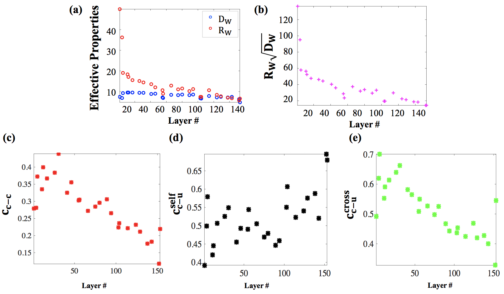
Figure 35: Analysis of Manifold Properties in Different Layers of Deep Networks. Using the ImageNet Dataset for different class as object manifolds, effective manifold properties were analyzed in different layers of GoogLeNet. (a) Effective Dimension $D_{W}$ and Effective Radius $R_{W}$ for different layers of GoogLeNet. (c) Half of Gaussian Mean Width $(R_{W}\sqrt{D_{W}}$) for different layers of GoogLeNet. (c) Correlation between manifold centers (d) Correlation between each manifold center and its axes, averaged over manifolds. (e) Correlation between each manifold center and the axes of the other manifolds, averaged over manifolds.

Interestingly, we find that the mean of the effective radius $R_{W}$ of ImageNet object manifolds decrease systematically while being processed by the layers of the deep network (Fig 35(a)). Particularly, the most dramatic improvement in $R_{W}$ appears in the early part of the processing. On the contrary, the mean effective dimension $D_{W}$ of ImageNet manifolds doesn’t decrease as significantly (Fig 35(a)). The values of $D_{W}$ at different layers are quite close to $2\text{log}m$ throughout (where $m$ is the number of training samples in each object class), and this may imply that the effective dimension of object manifolds is determined by the number of training samples of the data. Further investigations on what determines $D_{W}$ of the realistic data is ongoing work.

Recall that $R_{W}\sqrt{D_{W}}$, half of the Gaussian mean width, is directly related to the capacity of manifolds. There is a systematic drop in the size of $R_{W}\sqrt{D_{W}}$ across layers, where the most dramatic improvement is in the early stage and there is a consistent improvement in the rest of the layers (Fig 35(b)). Supposedly the utility of the deep structure of the network is increasing the manifold capacity, by reducing the Gaussian mean width.

Note that in $R_{W}$ and $R_{W}\sqrt{D_{W}}$, the best values are in the output (readout) layer, and the worst values are in the input (pixel) layer (Fig 35(a)-(b)).

Center-center correlations ($c_{c-c}$) also show systematic decrease across layers (Fig 35(c)), implying that deep network gradually decorrelates the centers of the object manifolds. Note that when there is more correlation between the centers, the total space spanned by the manifold centers will be more skewed (compared to spherical), and the effective ambient dimension spanned by the centers will be smaller, making the maximum critical number of manifolds smaller ^{litwin2017optimal}. Therefore, the deep network works towards increasing the manifold capacity by reducing the correlation between the centers. Other types of correlations (such as center to axes, within the manifold, $c_{c-u}^{self}$, or across manifolds, $c_{c-u}^{cross}$) show not as strong trends across the layers, and we hope to address this further in the future.

Future Work

In the future, we hope to connect the relationship between the theory and the experimental manifold capacity, and take into account various types of classifications, such as classification with sparse labels in the object recognition limit. Many deep networks have similar computational building blocks (i.e. convolution, max pooling, ReLu, dropouts, sparsity, etc), and we hope to address the role of each computational building block in terms of how they change the data manifolds. The change in the manifold shapes and manifold capacity during the learning is also an important future direction, in order to study what different types of learning can achieve in each layer, with a quantitative measure (manifold capacity). Finally, we hope to analyze the manifold representations in neural data, particularly in different areas of the brain (i.e. object representations in different stages of the visual hierarchy in the cortex^{dicarlo2007untangling}).

Appendix

Multi-Layer Networks with Sparse Intermediate Layer

In this section, we show the details for the numerical demonstrations shown in Section. Building Multi Layer Networks of Sparse Classifiers.

Training Two-Layer Network with Sparse Intermediate Layer

Input layer activity is $N$ dimensional and organized as manifolds such that they can be described as $\mathbf{z_{in}^{\mu}}=\mathbf{x_{0}}^{\mu}+R\sum_{i=1}^{D}s_{i}\mathbf{u}_{i}^{\mu}\in\mathbb{R}^{N}$ where subscript ’in’ denotes input layer, $\mathbf{x_{0}^{\mu}}$,$\mathbf{u}_{\mathbf{i}}^{\mathbf{\mu}}$,s,$R$ are from Linear Classification of Spherical Manifolds. We draw a set of i.i.d., random sparse binary labels $\{y_{i}^{\mu}\}$ (where $i=1,...,M$, $M$ being the dimensionality of the intermediate layer) with probability $f$ of being $1$. The output of the $i$-th nodes in the intermediate layer is binary $0,1$ with $z_{i}=\Theta\left[\mathbf{V}^{(i)}\cdot\mathbf{z_{in}}+b^{i}\right]$ where $\Theta(x)$ is Heaviside step function. The weight vector to the $i$ th node,$\mathbf{V}^{(i)}$ , and bias, $b^{i}$ are found as a max margin (SVM) solution for $D$-dimensional balls to the set of labeled pairs $\{\mathbf{z_{in}^{\mu}},y_{i}^{\mu}\}$, using the same method as in Algorithm 1. In Fig. 31, the network size used was $N=M=500$. Initial training data for the SVM solver for spheres had $m=2D$ samples per manifold, and then more points were added until the iteration converged (Algorithm 1). The output node is a linear readout of the intermediate layer representation, $z_{out}=\mbox{sign}\left[\bar{w}\cdot\bar{z}+b_{f}\right]$ . [We use overline to denote $M$-dim vectors.] The weight vector from second layer to the output node, $\bar{w}$ , and bias, $b_{f}$ (where subscript $f$ stands for final), is trained as an SVM solution to set of the labeled pairs, $\left\{\mathbf{z}^{\mu},y_{out}^{\mu}\right\}$, with the task dense labels $y_{out}^{\mu}=\pm 1$ with $f=0.5$. For details, see Algorithm 8.

Robustness to Input Noise

Once the two layered network is fully trained (without additive noise), we evaluate the probability of error in the output by adding additive full-rank gaussian noise (with standard deviation of $\sigma_{\mbox{noise}}$) to each input node and measuring the output node classification error as a function of the variance of the noise. For 31 (c), about 100 samples per manifold ($m$) were used and number of trials was 5. For details, see Alg. 8.

Robustness to Noise in the Intermediate Layer

We test the robustness to the introduction of smooth sigmoidal units in the intermediate layer, by first evaluating the intermediate weight matrix $\boldsymbol{V}$ to generate a sparse binary representation in the intermediate layer. After training of the intermediate layer, we replace the Heaviside step function of the intermediate layer nodes with $\Phi_{T}(x)=\left(1+e^{-x/T}\right)^{-1}$, which can be interpreted as the result of smoothing the binary function by stochastic noise. The readout weights are calculated as SVM solutions to the the densely labeled task pairs $\left\{\mathbf{z}^{\mu},y_{out}^{\mu}\right\}$ where $\boldsymbol{\mathbf{z}^{\mu}}$ are the intermediate layer sigmoidal responses to sampled inputs. For 31(d), about $100$ samples per manifold were used and number of trials was 5. The effect of the smoothness of the intermediate level on the classification performance of the binary output unit is measured as a function of the gain parameter $T$. For details, see Algorithm 8.

Initialize:

    $\mathbf{x_{0}}^{\mu},\mathbf{\vec{u}}^{\mu}\sim Norm(0,1)$ ( $\mu=1,...,P$) [Sample centers and direction vectors]

    $y_{\mbox{out}}^{\mu}\sim\mbox{sign}\left\{\mbox{Unif}(-1,1)\right\}$ ( $\mu=1,...,P$) [Sample dense labels for manifolds for output layer]

Train V (Input to Intermediate Layer):

    $s_{i}^{k,\mu}\sim\mbox{Unif}\left(-1,1\right)$ and $||\vec{s}^{k,\mu}||=1$ $i=1...D$,$k=1,...,m$, $\mu=1...P$. [Sample $m$ coefficient vectors from each manifold]

    repeat: for$j=1,...,M$ [for each node in intermediate layer]

        $\left(y^{\mu}\right)^{(j)}\sim P(y^{\mu})=f\delta(y^{\mu}-1)+(1-f)\delta(y^{\mu}+1).$ ($\mu=1,...,P$) [Sample sparse labels for manifolds for intermediate layer]

        $\mathbf{V}^{(j)},b^{(j)}$ = $M_{B}^{4}$($\mathbf{x_{0}}^{\mu},\mathbf{\vec{u}}^{\mu},\left(y^{\mu}\right)^{(i)},R$,$m$) [$M_{B}^{4}:$ $M^{4}$ algorithm for $L_{2}$ balls, see Chapter The Maximum Margin Manifold Machines]

    end

Train w (Intermediate to Output Layer):

    $s_{i}^{k,\mu}\sim\mbox{Unif}\left(-1,1\right)$ and $||\vec{s}^{k,\mu}||=1$ for all $i,k,\mu$

    $\mathbf{z}_{in}^{k,\mu}=$$\mathbf{x_{0}}^{\mu}+R\sum_{i=1}^{D}s_{i}^{k,\mu}\mbox{{u}}_{i}^{\mu}$ for all $\mu,k$ [Sample $m$ points on each manifold (first layer activity)]

   $z_{i}^{k,\mu}=\Theta\left[\mathbf{V}^{(i)}\cdot\mathbf{z_{in}}^{k,\mu}+b^{i}\right]$ for all $i=1,...,M$ and $k,\mu$ [Intermediate layer activity]

   $\bar{w},b_{f}=\mbox{svmsolver}(\bar{z}^{k,\mu},y_{out}^{k,\mu})$ [Find SVM solution with Intermediate layer activity and dense labels.]

Test Robustness to Input Noise (for $\sigma_{\mbox{noise}}$)

    $s_{i}^{k,\mu}\sim\mbox{Unif}\left(-1,1\right)$ and $||\vec{s}^{k,\mu}||=1$ for all $i,k,\mu$

    $\mathbf{z}_{in}^{k,\mu}=$$\mathbf{x_{0}}^{\mu}+R\sum_{i=1}^{D}s_{i}^{k,\mu}\mbox{{u}}_{i}^{\mu}+\eta$ , where $\eta\sim Norm(0,\sigma_{\mbox{noise}}I)$ for all $\mu,k$ [Sample $m$ points on each manifold with additive Gaussian noise (input layer activity with noise)]

   $z_{i}^{k,\mu}=\Theta\left[\mathbf{V}^{(i)}\cdot\mathbf{z_{in}}^{k,\mu}+b^{i}\right]$ for all $i,k,\mu$

   $z_{out}^{k,\mu}=\mbox{sign}\left[\bar{w}\cdot\bar{z}^{k,\mu}+b_{f}\right]$

   return: $\epsilon_{G}=\left\langle\frac{1}{4}\left(z_{out}^{k,\mu}-y_{out}^{k,\mu}\right)^{2}\right\rangle_{k,\mu,\mbox{trials}}$

Test Robustness to Noise in the Intermediate Layer (for $T\geq 0$)

    $s_{i}^{k,\mu}\sim\mbox{unif}\left(-1,1\right)$ and $||\vec{s}^{k,\mu}||=1$ for all $i,k,\mu$

    $\mathbf{z}_{in}^{k,\mu}=$$\mathbf{x_{0}}^{\mu}+R\sum_{i=1}^{D}s_{i}^{k,\mu}\mbox{{u}}_{i}^{\mu}$ for all $\mu,k$

   $z_{i}^{k,\mu}=\Phi_{T}\left[\mathbf{V}^{(i)}\cdot\mathbf{z_{in}}^{k,\mu}+b^{i}\right]$ for all $i,k,\mu$ [Use smooth sigmoid for intermediate layer]

   $\bar{w},b_{f},\kappa_{\mbox{margin}}=\mbox{svmsolver}(\bar{z}^{k,\mu},y_{out}^{k,\mu})$ [SVM solution for intermediate layer activity and labels]

   return: $\kappa_{\mbox{output}}\leftarrow\kappa_{\mbox{margin}}$ [Output margin with SVM solution]

Algorithm 8 Pseudocode for Two-Layer Network for Invariant Manifolds Classification

Appendix A: Symbols and Notations

Notations

$N$

Ambient Dimension for Data

$P$

Number of Manifolds

$D$

Embedding Dimension

$\kappa$

Margin

$R$

Radius of a ball

$R_{i}$

$i$ th radius of an ellipsoid ($i=1,...D$ for $D$ dimensional ellipsoid)

$\alpha=P/N$

Load (Number of Manifolds, $P$ /Ambient Dimension, $N$)

$\alpha_{C}$

Critical capacity (general expression)

$\alpha_{G}$,$\alpha_{0}$

Gardner’s perceptron capacity for points

$\alpha_{L}$

Capacity for Line Segments

$\alpha_{B}$,$\alpha_{B_{2}}$

Capacity for $L_{2}$ Balls

$\alpha_{B_{p}}$

Capacity for $L_{p}$ Balls

$\alpha_{E}$

Capacity for Ellipsoids

$\alpha_{M}$

Capacity for General Manifolds

$\alpha_{iter}$

Capacity for General Manifolds $\alpha_{M}$ found via iterative algorithm

$\alpha_{||}$

Capacity for Parallel Manifolds

$\mu,p$

Index of the $\mu$th ($p$th) manifold

$\mathbf{x}$

Point on a manifold

$\mathbf{x}_{0}$

Center of a manifold

$\mathbf{u_{i}}$

$i$ th basis vector of a manifold ($i=1,...,D$)

$\mathbf{v}$

$N$-dimensional vector $\mathbf{v}$ for an arbitrary vector

$\vec{v}$

$D$-dimensinoal vector $\vec{v}$ for an arbitrary vector

$\mathbf{w}$

Solution of a linear separating problem.

$b$

bias of a linear perceptron

$y$

binary ($\pm 1$) labels

$V$

Volume of space of solutions

$h_{0}$

field induced by a center of a manifold $\mathbf{x_{0}}$

$h_{i}$

field induced by the $i$ th axis of a manifold $\mathbf{u}_{i}$

$h$

field induced by a data point $\mathbf{x}$

$R_{E}$

Effective radius for an ellipsoid

$D_{E}$

Effective dimension for an ellispoid.

$R_{M}$

Effective manifold capacity radius for a general manifold (using self-consistent equations)

$D_{M}$

Effective manifold capacity dimension for a general manifold (using self-consistent equations)

$R_{W}$

Effective manifold capacity radius for a general manifold (using max projections on Gaussian vectors, related to the mean width)

$D_{W}$

Effective manifold capacity dimension for a general manifold (using max projections on Gaussian vectors)

$\epsilon_{g}$,$\epsilon_{G}$

Generalization error

$\epsilon_{t}$,$\epsilon_{T}$

Training error

$m$

number of subsamples per manifold

$\xi_{p}$

Slack parameter for the $p$th manifold

$s_{min}(\vec{v}),\tilde{s}(\vec{v})$

$\underset{\vec{s},f(\vec{s})=0}{argmin}\vec{s}\cdot\vec{v}$

$s^{*}$

$s$ solved via self-consistent equations on $z_{0}$ and $s$

$\kappa_{E}$

Excess margin for ellipsoids defined via $R_{E}\sqrt{D_{E}}$

$\kappa_{M}$

Excess margin for general manifolds defined via $R_{M}\sqrt{D_{M}}$

$\kappa_{W}$

Excess margin for general manifolds in scaling regime defined via $R_{W}\sqrt{D_{W}}$

$R_{c}$

Critical radius for phase transition

$d$

Embedding dimension per ambient dimension $D/N$

$\rho$

Overlap between the solution $\mathbf{w}$ and axes $\mathbf{u}_{i}$, $\frac{1}{D}\sum_{i=1}^{D}\left(\mathbf{w}\cdot\mathbf{u}_{i}\right)^{2}$

$f$

Sparsity of labels (Number of posive (or negative) labels/ Total number of labels)

$\kappa_{\text{int }}$

Margin in the intermediate layer unit (if intermediate unit is like a binary classifier)

$m$

Number of subsamples (training samples) per manifold

$M$

Intermediate layer size

Mathematical Conventions

$\left\|\mathbf{v}\right\|$

$L_{2}$ norm of a vector $\mathbf{v}$

$\left\|\mathbf{v}\right\|_{p}$

$L_{p}$ norm of a vector $\mathbf{v}$

$\Theta(x)$

Heaviside step function

$\langle X\rangle$

Average of a random variable $X$

$\langle\vec{x},\vec{y}\rangle$

Inner product between two vectors $\vec{x}$, $\vec{y}$

$\vec{x}\circ\vec{y}$

Hadamard (element-wise) product

$\left|S\right|$

Cardinality (number of elements) of a set $S$

$\left|x\right|$

Absolute value of a scalar $x$

$Dx$

Gaussian measure, $\frac{1}{\sqrt{2\pi}}e^{-\frac{1}{2}x^{2}}dx$

$\chi_{D}(t)$

Chi distribution, $\frac{2^{1-\frac{D}{2}}}{\Gamma(\frac{D}{2})}t^{D-1}e^{-\frac{1}{2}t^{2}}$

$H(x)$

$\int_{x}^{\infty}Dz=\frac{1}{\sqrt{2\pi}}\int_{x}^{\infty}dze^{-\frac{z^{2}}{2}}$

$\hat{v}$

$\vec{v}/||\vec{v}||$

$v$

$||\vec{v}||$

Appendix B: Gardner’s Replica Theory of Isolated Points

Consider a perceptron with $P$ input points $\mathbf{x}^{\mu}\in\mathbb{R}^{N}$ and $P$ labels $y^{\mu}=\pm 1$ , $\mu=1,...,P$. Assume that each component of$\mathbf{x}^{\mu}$ are Gaussian i.i.d. The weight plane $\mathbf{w\in\mathbb{R}^{N}}$ needs to classify all the input points such that all points are at least $\kappa$ away from the solution hyperplane. For simplicity, consider the regime where the number of positive labels and negative labels are equal. [This regime is called “dense classification” regime, where sparsity is $f=0.5$.] In this regime, optimal bias for maximum capacity is $b=0$ by symmetry, so let us ignore the bias term $b$ for now.

The problem is now to find $\mathbf{w}$ such that

$$h_{\mu}=\frac{y^{\mu}\mathbf{w}^{T}\mathbf{x}^{\mu}}{\sqrt{N}}>\kappa$$ (324)

where $\kappa$ is a margin. $h_{\mu}$, which we refer to as a field from a pattern $\mathbf{x}^{\mu}$ is a measure of distance between the pattern $\mathbf{x}^{\mu}$ and the solution hyperplane denoted by $\mathbf{w}$. Note that the denominator $\sqrt{N}$ is introduced so that $h_{\mu}$ does not grow with the network size $N$. In general, if $\mathbf{w}$ and $\mathbf{x}$ are random, then the scale of $\mathbf{w}^{T}\mathbf{x}$ is $\sqrt{N}$ . For now let us consider $\kappa=0$ case.

Gardner calculated $V$, which is the volume of solutions (weight vectors $\mathbf{w}$), which satisfy the classification constraint Eqn. 324 with $\kappa=0$. If $V$ goes to 0, then there is no solution and the network is beyond capacity. In order to compute $V$, each component of $w_{i}$ needs to be integrated with a term that is $0$ when the constraint is not satisfied, hence

$$V=\int d\mathbf{w}^{N}\delta(\mathbf{w}^{2}-N)\prod_{\mu=1}^{P}\Theta(h^{\mu})$$ (325)

where $\delta$ is a delta function, $\Theta$ is a Heaviside step fuction, and the norm on $\mathbf{w}$, $\delta(w^{2}-N)$, is imposed to count $\mathbf{w}$ in the same direction only once. Using the expression for the field (Eqn. 324), we get

$$V=\int dw^{N}\delta(w^{2}-N)\prod_{\mu=1}^{P}\Theta(\frac{y^{\mu}w^{T}x^{\mu}}{\sqrt{N}})$$ (326)

where $\Theta(h^{\mu})$ is one if $\mathbf{w}$ is a separating solution, and zero if it is not a solution, as the field (input to the $\Theta(x)$) will be negative.

Note that $V$ involves a product of many random contributions. Products of independent random numbers are known to possess distributions with long tails for which the average and the most probable value are markedly different. However, the logarithm of such quantities is a large sum of independent terms, hence is expected to have a Gaussian distribution so that its average and the most probable value match. Therefore, the most typical value of $V$ is expected to be

$$V_{typical}\sim\text{exp}\left[\langle\text{log}V\rangle\right]$$ (327)

Therefore, in order to get the typical behavior, we are interested in the average of log$V$ ^{engel2001statistical}. Hence, we need to calculate

$$\langle\log V\rangle_{x^{\mu}}$$ (328)

which is the average of $\log V$ over the quenched distribution of patterns. We can do this by the following formula:

$$\langle\log V\rangle=\lim_{n\rightarrow 0}\frac{\langle V^{n}\rangle-1}{n}$$ (329)

called “replica trick”, originally developed to calculate quenched averages in the theory of disordered solides.

Let us then calculate the expectation of $V^{n}$, which, in the case of a natural $n$, can be expanded as

$$\langle V^{n}\rangle=\langle\int\prod_{\alpha=1}^{n}dw^{\alpha}\delta(w_{\alpha}^{2}-N)\prod_{\mu}^{P}\prod_{\alpha}^{n}\Theta(h_{\alpha}^{\mu})\rangle_{x^{\mu}}$$ (330)

where $\alpha$ is an index for each one of the $n$ replicas of the original system with the same realization of random samples. We note that the question of how to go from a natural $n$ to the limit of $n\rightarrow 0$ is in general a hard problem, and more on this matter can be found in ^{mezard1988spin}.

We can replace $\Theta$ using the integral representation of the $\Theta$ function,

$$\langle\int\prod_{\alpha=1}^{n}dw^{\alpha}\delta(w_{\alpha}^{2}-N)\underbrace{\int_{\kappa}^{\infty}\prod_{\mu,\alpha}^{P,n}dh_{\mu}^{\alpha}\int_{-\infty}^{\infty}\prod_{\mu,\alpha}^{P,n}\frac{d\hat{h}_{\mu}^{\alpha}}{2\pi}e^{\frac{\left[i\hat{h}_{\mu}^{\alpha}h_{\mu}^{\alpha}-i\hat{h}_{\mu}^{\alpha}w^{\alpha T}x^{\mu}y^{\mu}\right]}{\sqrt{N}}}}_{C}\rangle_{x^{\mu}}$$ (331)

But because $\kappa=0$ and $\hat{h}>0$, we can change the range of the integrals to

$$\langle\int\prod_{\alpha=1}^{n}dw^{\alpha}\delta(w_{\alpha}^{2}-N)\underbrace{\int_{0}^{\infty}\prod_{\mu,\alpha}^{P,n}dh_{\mu}^{\alpha}\int_{0}^{\infty}\prod_{\mu,\alpha}^{P,n}\frac{d\hat{h}_{\mu}^{\alpha}}{2\pi}e^{\frac{\left[i\hat{h}_{\mu}^{\alpha}h_{\mu}^{\alpha}-i\hat{h}_{\mu}^{\alpha}w^{\alpha T}x^{\mu}y^{\mu}\right]}{\sqrt{N}}}}_{C}\rangle_{x^{\mu}}$$ (332)

(333)

Now average over the random patterns $x^{\mu}$only affect the term noted as $C$, that is,

$$C=\prod_{\mu=1}^{P}\int\prod_{\alpha=1}^{n}d\hat{h}_{\mu}^{\alpha}\int dh_{\mu}^{\alpha}\langle\prod_{\alpha=1}^{n}e^{\frac{-i\hat{h}_{\mu}^{\alpha}w^{\alpha T}x^{\mu}y^{\mu}}{\sqrt{N}}}\cdot e^{\frac{-i\hat{h}_{\mu}^{\alpha}h_{\mu}^{\alpha}}{\sqrt{N}}}\rangle_{x^{\mu}}$$ (334)

Now change the product of exponentials to the sum of powers, and taking out terms that don’t depend on $x^{\mu}$, we get

$$C=\prod_{\mu=1}^{P}\int\prod_{\alpha=1}^{n}d\hat{h}_{\mu}^{\alpha}\int dh_{\mu}^{\alpha}\langle e^{\sum_{\alpha=1}^{n}\frac{-i\hat{h}_{\mu}^{\alpha}w^{\alpha T}x^{\mu}y^{\mu}}{\sqrt{N}}}\rangle_{x^{\mu}}\cdot e^{\frac{-i\hat{h}_{\mu}^{\alpha}h_{\mu}^{\alpha}}{\sqrt{N}}}$$ (335)

Since $w^{\alpha}$ is a vector, we expand the vector dot product $w^{\alpha T}x^{\mu}$ as sum of each vector’s elements, then

$$C=\prod_{\mu=1}^{P}\int\prod_{\alpha=1}^{n}d\hat{h}_{\mu}^{\alpha}\int dh_{\mu}^{\alpha}\langle e^{\frac{\sum_{\alpha=1}^{n}-i\hat{h}_{\mu}^{\alpha}\sum_{j}w_{j}^{\alpha}x_{j}^{\mu}y^{\mu}}{\sqrt{N}}}\rangle_{x^{\mu}}\cdot e^{\frac{-i\hat{h}_{\mu}^{\alpha}h_{\mu}^{\alpha}}{\sqrt{N}}}$$ (336)

Then the sum $\sum_{j}$ in the power can be the product of exponentials, then

$$C=\prod_{\mu=1}^{P}\int\prod_{\alpha=1}^{n}d\hat{h}_{\mu}^{\alpha}\int dh_{\mu}^{\alpha}\langle\prod_{j}e^{\frac{-i\sum_{\alpha=1}^{n}\hat{h}_{\mu}^{\alpha}w_{j}^{\alpha}x_{j}^{\mu}y^{\mu}}{\sqrt{N}}}\rangle_{x^{\mu}}\cdot e^{\frac{-i\hat{h}_{\mu}^{\alpha}h_{\mu}^{\alpha}}{\sqrt{N}}}$$ (337)

Becasue each element is independent, we can take out product over j

$$C=\prod_{\mu=1}^{P}\int\prod_{\alpha=1}^{n}d\hat{h}_{\mu}^{\alpha}\int dh_{\mu}^{\alpha}\prod_{j}\langle e^{\frac{-i\sum_{\alpha=1}^{n}\hat{h}_{\mu}^{\alpha}w_{j}^{\alpha}x_{j}^{\mu}y^{\mu}}{\sqrt{N}}}\rangle_{x_{j}^{\mu}}\cdot e^{\frac{-i\hat{h}_{\mu}^{\alpha}h_{\mu}^{\alpha}}{\sqrt{N}}}$$ (338)

Now use the fact that $\int Dxe^{ixA}=e^{-A^{2}/2}$ , we get rid of $\langle\rangle_{x}\sim\int Dx$ . Note that $A^{2}$ is like

$$\left(\sum_{\alpha}\left(-y^{\mu}\right)\frac{\hat{h}_{\mu}^{\alpha}w_{j}^{\alpha}}{\sqrt{N}}\right)^{2}=\left(\sum_{\alpha}\frac{\hat{h}_{\mu}^{\alpha}w_{j}^{\alpha}}{\sqrt{N}}\right)^{2}=\frac{\left(\sum_{\alpha}\hat{h}_{\mu}^{\alpha}w_{j}^{\alpha}\right)^{2}}{N}$$ (339)

So we have:

$$C=\prod_{\mu=1}^{P}\int\prod_{\alpha=1}^{n}d\hat{h}_{\mu}^{\alpha}\int dh_{\mu}^{\alpha}\prod_{j=1}^{N}e^{\frac{-\left(\sum_{\alpha=1}^{n}\hat{h}_{\mu}^{\alpha}w_{j}^{\alpha}\right)^{2}}{2N}}\cdot e^{\frac{-i\hat{h}_{\mu}^{\alpha}h_{\mu}^{\alpha}}{\sqrt{N}}}$$ (340)

which can be re-written as

$$C=\prod_{\mu=1}^{P}\int\prod_{\alpha=1}^{n}d\hat{h}_{\mu}^{\alpha}\int dh_{\mu}^{\alpha}\prod_{j=1}^{N}e^{\frac{-\sum_{\alpha,\beta=1}^{n}\hat{h}_{\mu}^{\alpha}\hat{h}_{\mu}^{\beta}w_{j}^{\alpha}w_{j}^{\beta}}{2N}}\cdot e^{\frac{-i\hat{h}_{\mu}^{\alpha}h_{\mu}^{\alpha}}{\sqrt{N}}}$$ (341)

Define $q_{\alpha\beta}=\frac{1}{N}\sum_{j}w_{j}^{\alpha}w_{j}^{\beta}$ which is the replica symmetric order parameter.

$$C=\prod_{\mu=1}^{P}\int\prod_{\alpha=1}^{n}d\hat{h}_{\mu}^{\alpha}\int dh_{\mu}^{\alpha}\underbrace{e^{-\frac{1}{2}\left(\sum_{\alpha=1}^{n}\sum_{\beta=1}^{n}\hat{h}_{\mu}^{\alpha}q_{\alpha\beta}^{-1}\hat{h}_{\mu}^{\beta}\right)}}_{X}\cdot e^{\frac{-i\hat{h}_{\mu}^{\alpha}h_{\mu}^{\alpha}}{\sqrt{N}}}$$ (342)

Define

$$X(\hat{h}_{\mu}^{\alpha})=e^{-\frac{1}{2}\left(\sum_{\alpha,\beta=1}^{n}\hat{h}_{\mu}^{\alpha}q_{\alpha\beta}^{-1}\hat{h}_{\mu}^{\beta}\right)}$$ (343)

$$C=\prod_{\mu=1}^{P}\int_{0}^{\infty}\prod_{\alpha=1}^{n}dh_{\mu}^{\alpha}\left[\int_{0}^{\infty}\prod_{\alpha=1}^{n}d\hat{h}_{\mu}^{\alpha}X(\hat{h}_{\mu}^{\alpha},....)e^{\frac{-i\hat{h}_{\mu}^{\alpha}h_{\mu}^{\alpha}}{\sqrt{N}}}\right]$$ (344)

(Here we changed the orders of $h$ and $\hat{h}$.)

By integrating out $d\hat{h}$, we get

$$C=\prod_{\mu=1}^{P}\int_{0}^{\infty}\prod_{\alpha=1}^{n}dh_{\mu}^{\alpha}\left[X(\hat{h}_{\mu}^{\alpha}=h_{\mu}^{\alpha})\frac{1}{\sqrt{\det q}}\right]$$ (345)

where we used the delta function identity, Eqn. 343,( $X(\hat{h}_{\mu}^{\alpha}=h_{\mu}^{\alpha})$) and n-dimensional Gaussian integration with matrix $q$ to get $\frac{1}{\sqrt{\det q}}$ term. We re-write Eqn. 345 such that:

$$C=\prod_{\mu=1}^{P}\int_{0}^{\infty}\prod_{\alpha=1}^{n}dh_{\mu}^{\alpha}\left[X(\hat{h}_{\mu}^{\alpha}=h_{\mu}^{\alpha})e^{-\frac{1}{2}\log\det q}\right]$$ (346)

which is:

$$C=\prod_{\mu=1}^{P}\int_{0}^{\infty}\prod_{\alpha=1}^{n}dh_{\mu}^{\alpha}\left[[\underbrace{e^{-\frac{1}{2}\left(\sum_{\alpha,\beta=1}^{n}h_{\mu}^{\alpha}q_{\alpha\beta}^{-1}h_{\mu}^{\beta}\right)}}_{X}]e^{-\frac{1}{2}\log\det q}\right]$$ (347)

where

$$X=e^{-\frac{1}{2}\left(\sum_{\alpha,\beta=1}^{n}h_{\mu}^{\alpha}q_{\alpha\beta}^{-1}h_{\mu}^{\beta}\right)}$$ (348)

Then, $C$ can be simplied with $X$,

$$C=\prod_{\mu=1}^{P}\int_{0}^{\infty}\prod_{\alpha=1}^{n}dh_{\mu}^{\alpha}\left[Xe^{-\frac{1}{2}\log\det q}\right]$$ (349)

Now going back to $\langle V^{N}\rangle$, in Eqn. 332, is now (after the above calculations):

$$\langle V^{N}\rangle=\left\langle\int\prod_{\alpha=1}^{N}dw^{\alpha}\delta(w_{\alpha}^{2}-N)\underbrace{\prod_{\mu=1}^{P}\left[\int_{0}^{\infty}\prod_{\alpha=1}^{P}dh_{\mu}^{\alpha}Xe^{-\frac{1}{2}\log\det q}\right]}_{C}\right\rangle$$ (350)

where $X$ is given as Eqn. 348. We note that the term $C$ has two parts

$$C(X)=\prod_{\mu=1}^{P}\int_{0}^{\infty}\prod_{\alpha=1}^{P}dh_{\mu}^{\alpha}\underbrace{\left\{e^{-\frac{1}{2}\left(\sum_{\alpha,\beta=1}^{n}h_{\mu}^{\alpha}q_{\alpha\beta}^{-1}h_{\mu}^{\beta}\right)}\right\}}_{X}$$ (351)

and

$$C(0)=e^{-\frac{P}{2}\log\det q}$$ (352)

for later use.

Because it’s an integral of $q_{\alpha\beta}=\frac{1}{N}\sum_{j}w_{j}^{\alpha}w_{j}^{\beta}=q_{\alpha\beta}(w)$ which is a complex function of $w$, we write it in terms of integral of deltas of $q_{\alpha\beta}$. Intuitively, $q$ is generally thought of as a function of the overlaps between the solution of weights.

Now, we can re-write the $\langle V^{N}\rangle$ as functions of $q_{\alpha\beta}$ , by introducing

$$\int dq_{\alpha\beta}d\hat{q}_{\alpha\beta}e^{i\hat{q}_{\alpha\beta}\left(-q_{\alpha\beta}N+\sum_{j}w_{j}^{\alpha}w_{j}^{\beta}\right)}$$ (353)

And we get:

$$\langle V^{n}\rangle =\int dq_{\alpha\beta}d\hat{q}_{\alpha\beta}\int\prod_{\alpha=1}^{n}dw^{\alpha}\left[\delta(w_{\alpha}^{2}-N)\right.$$ (354)

$$\left.e^{-iq_{\alpha\beta}\hat{q}_{\alpha\beta}N}e^{i\hat{q}_{\alpha\beta}\sum_{j}w_{j}^{\alpha}w_{j}^{\beta}}e^{-\frac{P}{2}\log\det q}C(X)\right]$$ (355)

where $C(X)$ is defined in Eqn. 351.

Let us use the replica symmetric ansatz

$$q_{\alpha\beta}=(1-q)\delta_{\alpha\beta}+q$$ (356)

Now going back to evaluating $C(X)$,

$$C(X)=\prod_{\mu=1}^{P}\int_{0}^{\infty}\prod_{\alpha}dh_{\mu}^{\alpha}[e^{-\frac{1}{2}\left(\sum_{\alpha,\beta=1}^{n}h_{\mu}^{\alpha}q_{\alpha\beta}^{-1}h_{\mu}^{\beta}\right)}]$$ (357)

where, given our ansatz (Eqn. 356),

$$q^{-1}_{\alpha\beta}=\frac{1}{1-q}\delta_{\alpha\beta}+\left(\frac{-q}{\left(1-q\right)\left(1+(n-1)q\right)}\right)$$ (358)

where $n$ is a dimension of the matrix. However, we are in the limit $n\rightarrow 0$, therefore

$$q^{-1}_{\alpha\beta}=\frac{1}{1-q}\delta_{\alpha\beta}+\frac{-q}{(1-q)^{2}}$$ (359)

With Eqn. 359, Eqn. 357 becomes

$$C(X)=\prod_{\mu=1}^{P}\int_{0}^{\infty}\prod_{\alpha=1}^{n}dh_{\mu}^{\alpha}[e^{-\frac{1}{2(1-q)}\sum_{\alpha}\left(h_{\mu}^{\alpha}\right)^{2}+\frac{q}{2(1-q)^{2}}\left(\sum_{\alpha}h_{\mu}^{\alpha}\right)^{2}}]$$ (360)

Let us introduce $h^{\prime}=\frac{h}{\sqrt{1-q}}$ (for simplicity), then

$$C(X)=\prod_{\mu=1}^{P}\int_{0}^{\infty}\prod_{\alpha=1}^{n}dh{}_{\mu}^{\prime\alpha}[e^{-\frac{1}{2}\sum_{\alpha}\left(h_{\mu}^{\prime\alpha}\right)^{2}+\frac{q}{2(1-q)}\left(\sum_{\alpha}h{}_{\mu}^{\prime\alpha}\right)^{2}}]$$ (361)

Using Hubbard–Stratonovich transformation, $e^{A^{2}/2}=\int_{-\infty}^{\infty}\frac{dt}{\sqrt{2\pi}}e^{-\frac{1}{2}t^{2}+At}$, we introduce additional expansion,

$$C(X)=\prod_{\mu=1}^{P}\int Dt_{\mu}\prod_{\alpha=1}^{n}\int_{0}^{\infty}dh{}_{\mu}^{\prime\alpha}[e^{-\frac{1}{2}\sum_{\alpha}\left(h_{\mu}^{\prime\alpha}\right)^{2}+\sqrt{\frac{q}{1-q}}t_{\mu}\sum_{\alpha}h{}_{\mu}^{\prime\alpha}}]$$ (362)

which, finally, can be simplified to

$$C(X)=\prod_{\mu=1}^{P}\int Dt_{\mu}\left\{\int_{0}^{\infty}dh{}_{\mu}^{\prime\alpha}[e^{-\frac{1}{2}\left(h_{\mu}^{\prime\alpha}\right)^{2}+\sqrt{\frac{q}{1-q}}t_{\mu}h{}_{\mu}^{\prime\alpha}}]\right\}^{n}$$ (363)

In other words,

$$C(X)=\prod_{\mu=1}^{P}\int Dt_{\mu}\left[\ e^{\log Z(t_{\mu},q)}\right]^{n}$$ (364)

where

$$Z(t_{\mu},\>q)=\int_{0}^{\infty}\frac{dh}{\sqrt{2\pi}}[e^{-\frac{1}{2}h^{2}+\sqrt{\frac{q}{1-q}}t_{\mu}h}]$$ (365)

Now

$$C(X)=\left[\int Dt\ e^{n\log Z(t,q)}\right]^{P}$$ (366)

And by simple power expansion,

$$C(X)=e^{P\log\left(1+n\langle\log Z(t,q)\rangle\right)}$$ (367)

Expanding log, we get:

$$C(X)=e^{Pn\langle\log Z(t,q)\rangle}$$ (368)

Note, we are trying to evaluate

$$\langle\log V\rangle=\lim_{n\rightarrow 0}\frac{\langle V^{n}\rangle-1}{n}$$ (369)

by using Eqn. 350 and which has $C(X)$ (Eqn.351) and $C(0)$ (Eqn. 352). We need to now evaluate $C(0)$ with Eqn. 352.

Now, noting that $\mbox{$\log$det}q_{\alpha\beta}$ is related to the sum of log of eigenvalues,

$$\log\det q_{\alpha\beta}=\sum_{l}\log\lambda_{l}$$ (370)

where $\lambda_{l}$, $l=1,...$ are eigenvalues of $q_{\alpha\beta}$. With the replica symmetric ansatz of $q_{\alpha\beta}$ is given by Eqn. 356, the first eigenvalues are $1+(n-1)q$ and the rest of the $(n-1)$ eigenvalues are $1-q$ ,

Therefore

$$\log\det q=n\log\left(1-q\right)+\frac{nq}{\left(1-q\right)}$$ (371)

where the linear term in $n$ is dominant. Then,using Eqn. 371, $C(0)$ from Eqn. 352 is now,

$$C(0)=\mbox{exp}\left(-\frac{1}{2}Pn\log\left(1-q\right)-\frac{1}{2}\frac{Pnq}{\left(1-q\right)}\right)$$ (372)

Now, back to the original equation.

$$\langle V^{n}\rangle =\int dq_{\alpha\beta}d\hat{q}_{\alpha\beta}\int\prod_{\alpha=1}^{n}dw^{\alpha}\left[\delta(w_{\alpha}^{2}-N)\right.$$ (373)

$$\left.e^{-iq_{\alpha\beta}\hat{q}_{\alpha\beta}N}e^{i\hat{q}_{\alpha\beta}\sum_{j}w_{j}^{\alpha}w_{j}^{\beta}}C(0)C(X)\right]$$ (374)

Expanding $\delta(w_{\alpha}^{2}-N)$ to an exponential form with a new variable $\lambda_{\alpha}$:

$$\langle V^{n}\rangle =\int dq_{\alpha\beta}d\hat{q}_{\alpha\beta}\int\prod_{\alpha}d\lambda_{\alpha}\int\prod_{\alpha=1}^{n}dw^{\alpha}\text{exp}\Biggl{\{}i\lambda_{\alpha}(w_{\alpha}^{2}-N)$$ (375)

$$\left.-iq_{\alpha\beta}\hat{q}_{\alpha\beta}N+i\hat{q}_{\alpha\beta}\sum_{j}w_{j}^{\alpha}w_{j}^{\beta}\right\}C(0)C(X)$$ (376)

We change the definition of $C(X)$ slightly, so that

$$C(X)=e^{Pn\langle\log Z(t,q)\rangle}=e^{\alpha Nn\langle\log Z(t,q)\rangle}$$ (377)

where

$$\alpha=P/N$$ (378)

is the capacity we wish to get.

Doing the integral over $w^{\alpha}$ gives the term:

$$e^{\left\{-\frac{N}{2}\log\det\left[\lambda_{\alpha}\delta_{\alpha\beta}+\hat{q}_{\alpha\beta}\right]\right\}}$$ (379)

And absorbing $i$ into the new variable, that is, use $\lambda\leftarrow i\lambda$, we get,

$$\langle V^{n}\rangle=\int dq_{\alpha\beta}d\hat{q}_{\alpha\beta}\int d\lambda_{\alpha}\text{exp}\left[F(q_{\alpha\beta},\hat{q}_{\alpha\beta},\lambda_{\alpha})\right]$$ (380) where $$F=-\lambda_{\alpha}N+q_{\alpha\beta}\hat{q}_{\alpha\beta}N-\frac{N}{2}\log\det\left[\lambda_{\alpha}\delta_{\alpha\beta}+\hat{q}_{\alpha\beta}\right]+\alpha Nn\langle\log Z(t,q)\rangle$$ (381)

Where the dependence is only on non-local variables like $N$, $P$, $n\rightarrow 0$. Let us now evaluate the integral using the saddle point approximation,

$$I=\int dx\text{exp}\left[-g(x)\right]\sim\text{exp}\left[-g(x_{0})\right]\sqrt{\frac{2\pi}{g^{\prime\prime}(x_{0})}}$$ (382)

where$g(x)$ is at its minimum at $x_{0}$ .

In the limit of $N\rightarrow\infty$, we can use the following ansatz assuming replica symmetry,

$$q_{\alpha\beta}=(1-q)\delta_{\alpha\beta}+q$$ (383)

$$\hat{q}_{\alpha\beta}=\left(\hat{q}_{0}-\hat{q_{1}}\right)\delta_{\alpha\beta}+\hat{q_{1}}$$ (384)

where we denote $\hat{q}_{0}-\hat{q_{1}}$ as $\Delta\hat{q}$, and find the saddle point by taking the derivative of $F$

$\frac{\partial F}{\partial\lambda_{\alpha}}=0:$

$$1=\frac{1}{\lambda+\Delta\hat{q}}-\frac{\hat{q}_{1}}{\left(\lambda+\Delta\hat{q}\right)^{2}}$$ (385)

$\frac{\partial F}{\partial\hat{q}_{\alpha\beta}}=0:$

$$q_{\alpha\beta}=\left(1-q\right)\delta_{\alpha\beta}+q=\left(\frac{1}{\lambda+\Delta\hat{q}}\right)\delta_{\alpha\beta}-\frac{\hat{q}_{1}}{\left(\lambda+\Delta\hat{q}\right)^{2}}$$ (386)

Thus, we get

$$q=\frac{-\hat{q_{1}}}{\left(\lambda+\Delta\hat{q}\right)^{2}}$$ (387)

Note that doing saddle points with $\lambda$ and $\hat{q}$ are easier, and we did these operations first. Then, from Eqn. 385, we obtain

$$1=\frac{1}{\lambda+\Delta\hat{q}}+q$$ (388)

If we go back to the original equation, Eqn. 380, and plug in back the saddle points, then, we get

$$\frac{Nn}{2}\left[\left(\lambda+\Delta\hat{q}\right)-\log\left(\lambda+\Delta\hat{q}\right)\right]+Nn\alpha\langle\log Z(t,q)\rangle$$ (389)

which eventually leads us to the expression for the term

$$\langle V^{n}\rangle=e^{Nn\left[G_{0}(q)+\alpha G_{1}(q)\right]}$$ (390)

where

$$G_{0}(q)=\frac{1}{2}\left[\frac{1}{1-q}+\log\left(1-q\right)\right]$$ (391) $$G_{1}(q)=\langle\log\underbrace{\int_{0}^{\infty}\frac{dh}{\sqrt{2\pi}}e^{-\frac{1}{2}\left(h-\sqrt{\frac{q}{1-q}}t\right)^{2}}}_{H(\sqrt{\frac{q}{1-q}}t)=H(\sqrt{Q}t)}\rangle_{t}=\langle\log H(\sqrt{Q}t)\rangle_{t}$$ (392)

Note that $G_{0}$ is an entropic term and doesn’t change with constraints, but for classification with additional constraints (such as manifolds classification), $G_{1}$ does change and and computing $\langle\log H(\sqrt{Q}t)\rangle_{t}$ becomes important.

Therefore, by L’Hospital’s rule, we get in the limit of $n\rightarrow 0$,

$$\langle\log V\rangle=N\left[G_{0}(q)+\alpha G_{1}(q)\right]$$ (393)

Note that $G_{0}$ is an entropic term, and $G_{1}$ needs to be self-consistent.

$$\frac{\partial G_{0}}{\partial q}=\frac{q}{2(1-q)^{2}}$$ (394)

$$\alpha\frac{\partial G_{1}}{\partial q}=\alpha\frac{\partial Q}{\partial q}\frac{\partial G_{1}}{\partial Q}$$ (395)

Now plugging the expressions back to the self-consistency requirement ($\frac{\partial G_{0}}{\partial q}=\alpha\frac{\partial G_{1}}{\partial q}$) we get:

$$1=\frac{\alpha(1-q)}{q}\langle\left(\frac{e^{-Qt^{2}/2}}{\sqrt{2\pi}H(\sqrt{Q}t)}\right)^{2}\rangle_{t}$$ (396)

And the final step for capacity is we send $q\rightarrow 1$ ($Q\rightarrow\infty$) because there is only one solution and in this limit the overlap is 1. With such limit, we get $\alpha=2$ , which is the capacity of isolated points for zero-margin solution.

Remarks. If $\alpha=0$ then $q$ has to be zero from Eqn 396. Intuitively, this means that as the number of points $P$ approach zero (or the network size $N$ approaches infinity compared to the number of points $P$), the problem becomes very easy and there is a lot of solutions, making the overlap between solutions $q$ go to 0.