On Optimizing the Conditional Value-at-Risk of a Maximum Cost for Risk-Averse Safety Analysis*
Abstract
The popularity of Conditional Value-at-Risk (CVaR), a risk functional from finance, has been growing in the control systems community due to its intuitive interpretation and axiomatic foundation. We consider a nonstandard optimal control problem in which the goal is to minimize the CVaR of a maximum random cost subject to a Borel-space Markov decision process. The objective represents the maximum departure from a desired operating region averaged over a given fraction of the worst cases. This problem provides a safety criterion for a stochastic system that is informed by both the probability and severity of the potential consequences of the system’s behavior. In contrast, existing safety analysis frameworks apply stage-wise risk constraints or assess the probability of constraint violation without quantifying the potential severity of the violation. To the best of our knowledge, the problem of interest has not been solved. To solve the problem, we propose and study a family of stochastic dynamic programs on an augmented state space. We prove that the optimal CVaR of a maximum random cost enjoys an equivalent representation in terms of the solutions to these dynamic programs under appropriate assumptions. For each dynamic program, we show the existence of an optimal policy that depends on the dynamics of an augmented state under the assumptions. In a numerical example, we illustrate how our safety analysis framework is useful for assessing the severity of combined sewer overflows under precipitation uncertainty.
Conditional Value-at-Risk, Risk-averse optimal control, Safety analysis, Markov decision processes.
1 Introduction
Control system safety is often assessed through minimax optimal control problems [1, 2, 3, 4], which assume bounded nonstochastic adversarial disturbances that try to inhibit safe or efficient operation. In cases where disturbances are not well-modeled as bounded inputs (e.g., Gaussian noise), then it is standard to define safety in terms of a stochastic optimal control problem, whose optimal value is a probability of satisfactory operation. This framework, called stochastic safety analysis, can accommodate either adversarial [5, 6] or nonadversarial [7, 8] stochastic disturbances. However, a minimax approach may lead to controllers that are too cautious in practice. On the other hand, a purely probabilistic risk assessment indicates the likelihood of a harmful event but has a limited capacity to quantify the amount of harm the event would cause. These different limitations have motivated a growing body of research that lies in the intersection of formal methods and risk analysis for control systems [9, 10, 11, 12, 13].
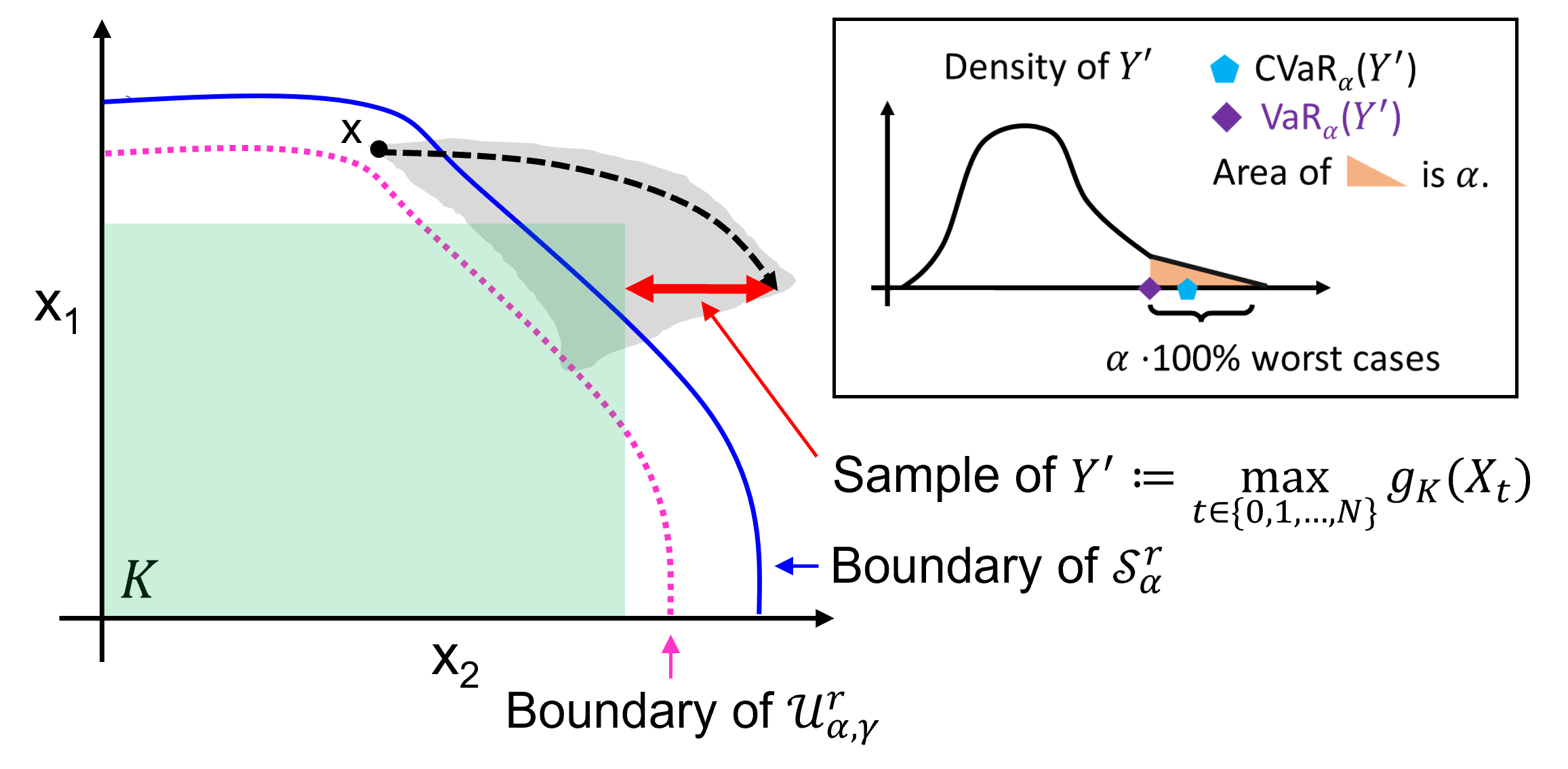
Here, we study a nonstandard safety analysis problem, which concerns the notion of a risk-averse safe set . represents the set of initial states from which the maximum distance between the trajectory and a desired operating region averaged over the worst cases can be reduced to a threshold (Fig. 1). The system of interest is a Markov decision process (MDP) with Borel spaces of states, controls, and disturbances, operating on a discrete-time horizon of length , a natural number. is the optimal value of a stochastic optimal control problem with a Conditional Value-at-Risk maximum cost objective:
| (1a) | ||||
| (1b) | ||||
The random variable depends on stage and terminal cost functions , random states , and random controls . The quantity represents the average value of in the worst cases when the initial state is and the system uses the control policy . A control policy provides distributions for the realizations of . (We will formalize and in Sec. 3.2 and Sec. 4.1, respectively.) The setting is fairly general in theory. It permits nonlinear dynamics, nonconvex bounded cost functions, continuous spaces, and non-Gaussian stochastic disturbances. First, we will explain why (1) is an important problem to solve, and then we will explain the novelty of our contribution.
1.1 Relevance of the CVaR
The CVaR functional, which defines the objective of (1), provides an intuitive and quantitative interpretation for risk because it represents the average value of a random variable in a fraction of the worst cases [24, Th. 6.2]. Other common risk functionals do not have interpretations that are as consistent or clear. Expected utility risk functionals encode risk preferences using utility functions and their parameters [14, 15, 16, 17, 18, 19]. It is challenging to provide a precise meaning for the parameter of the classical expected exponential utility functional, which limits its applicability to control systems with specific safety or performance requirements [20]. It may be difficult to interpret a recursive risk functional because it takes the form , where is a random variable and is a map between spaces of random variables [21, 22, 23]. A weighted sum of the mean and a moment-based dispersion functional, e.g., variance, standard deviation, and upper-semideviation [24], provides an heuristic for the probability and severity of more rare and harmful outcomes. The CVaR is arguably more intuitive than the broader class of spectral risk functionals, which are “mixtures” of the CVaRα over the values of [25, Prop. 2.5]. The Value-at-Risk (VaR) at level , which is the left-side -quantile, has a clear quantitative interpretation. However, the VaR’s ability to summarize the severity of harmful outcomes is limited because it is insensitive to the shape of the distribution beyond the ()-quantile. From a decision-theoretic perspective, the VaR has the disadvantage of lacking a desirable property called subadditivity [26]. Both of these shortcomings are overcome by the CVaR [27, 24].
1.2 Relevance of the Maximum Cost
We focus on a maximum cost (1b) generated by an MDP rather than a cumulative cost. While a cumulative cost is typical for MDP problems [17, 28, 21, 29, 30, 23, 25], a maximum cost is typical for robust safety and reachability analysis problems for nonstochastic systems, e.g., see [3, 4], and the references therein. Maximum costs have natural roles in systems theory, beyond robust safety and reachability analysis. The theory of the long-term behavior of normalized maxima of random variables, i.e., extreme value theory, has applications in finance, the study of human longevity, and hydrology [31].
A maximum cost is appropriate for applications in which the extent of a constraint violation over a brief time interval is more critical to assess than its accumulation.111A constraint violation means that a state or control leaves a desired operating region, and its extent refers to the severity of the violation. For example, in stormwater management, the maximum water level can be a useful surrogate for the maximum flood extent (in more extreme cases) and the maximum discharge rate (in general). These are instantaneous rather than cumulative properties. For gravity-drained stormwater systems, the instantaneous discharge rate through an uncontrolled outlet into open atmosphere is a function of the water level behind the outlet. Therefore, from water levels, we can estimate instantaneous demands on downstream conveyance infrastructure (i.e., infrastructure to transport water rather than to store it). Designing this infrastructure for the worst maximum discharge rate may be cost-prohibitive. However, assessing the average maximum water level in the worst of cases from historical data would allow designers to estimate downstream conveyance capacity demands along a spectrum of worst cases.
1.3 Related Literature
The problem of computing risk-averse safe sets is distinct from established problems in the stochastic and risk-averse control theory literature and necessitates different techniques. Classical discrete-time stochastic control theory, e.g., [32], studies the problem of optimizing the expectation of a cumulative cost. In contrast, our focus is optimizing the CVaR of a maximum cost (1). The dynamic programming (DP) proofs from stochastic control theory do not apply to our problem directly. Theoretical challenges arise because the CVaR satisfies only some of the properties that are enjoyed by the expectation. Moreover, while sums and integrals of nonnegative Borel-measurable functions can be interchanged, this is not the case for maxima and integrals in general. Such technical differences between our problem and the scenarios that prevail in the literature make it necessary to build a pathway from measure-theoretic first principles. Doing so enables us to solve for the sets and the associated optimal control policies under appropriate assumptions.
We take inspiration from a technique called state-space augmentation, which has been used to solve risk-averse MDP problems with cumulative costs [28, 17, 29, 30, 25]. The problem of minimizing the expectation of a cumulative cost subject to an upper bound on the CVaR of a cumulative cost has been studied in [29]. The authors propose offline and online algorithms on augmented state spaces to update a Lagrange multiplier and a lower bound on a cumulative cost [29]. Several risk-averse control problems with cumulative costs over an infinite time horizon have been investigated using infinite-dimensional linear programming and state-space augmentation [30]. Bäuerle and Ott provide a DP solution to the problem of minimizing the CVaR of a cumulative cost [28]. While we also use DP, our approach requires different proof techniques to manage a maximum cost (1b) and to study our proposed algorithm, which we define in terms of dynamics functions , stage and terminal cost functions , and disturbance distributions .
Most literature about risk-averse MDPs concerns exponential utility, taking inspiration from decision theory in economics and extending from 1972 to present-day [14, 15, 16, 33, 18, 19]. Bäuerle and Rieder study the problem of optimizing an expected utility for systems on Borel spaces with state-space augmentation, analyzing exponential utility as a special case [17]. Another line of work considers the optimization of recursive risk functionals [21, 33, 22, 23]; the basic approach is to replace a conditional expectation with a “conditional risk functional” to derive a risk-based Bellman equation. The problem of minimizing an expected cumulative cost subject to a risk constraint has been studied by, e.g., [29, 30, 40, 35, 11, 9]. Linear-quadratic settings have been studied in [40, 35, 11], and a safety analysis problem with CVaR has been proposed by [9]. Our problem (1) assesses the risk of the entire trajectory, whereas the framework in [9] is concerned with the risk of each state in the trajectory separately, i.e., must be small for every . An emerging research direction proposes risk-averse signal temporal logic specifications for linear-quadratic model predictive control [11] and for a setting with continuous-time systems of the form [13]. We refer the reader to our survey about risk-averse autonomous systems [34] and the references therein for additional literature.
Contributions. We show that any collection of risk-averse safe sets is characterized exactly using the solutions to a family of stochastic dynamic programs on an augmented state space under a measurable selection assumption. We derive this characterization by expressing the minimum CVaR (for a given initial state and a given level ) as a nested optimization problem with respect to a control policy and a dual parameter . We propose a nonstandard stochastic dynamic program that is parametrized by to assess a maximum random cost. We show that the algorithm returns an optimal -dependent value function and policy under regularity conditions on the dynamics functions, stage and terminal cost functions, and disturbance distributions. Subsequently, we perform an outer minimization over to obtain (1). The framework permits nonlinear dynamics, non-Gaussian noise, nonconvex bounded cost functions, and continuous spaces. We solve the risk-averse safety analysis problem, whereas our prior works [10, 12] provide approximations. For detailed derivations of our theory, we refer the interested reader to the Appendix.
The numerical tractability of the method is limited due to its reliance on DP and an augmented state space. In this work, we provide a nonlinear two-dimensional example motivated by a stormwater management application and offer a comparison to our underapproximation method from [12]. Our on-going and future work involves developing more scalable approaches using extreme value theory and value function approximations.
Notation. We define and . Given , we define and . If is a metrizable space, then is the Borel sigma algebra on . If , then means that there is a point such that ; i.e., attains its infimum, and is a minimizer. If , where is a metrizable space, then we define by . If is a Borel space, then is the space of probability measures on with the weak topology; if , then is the Dirac measure in that is concentrated at . We distinguish between random objects and their realizations (i.e., values) using capital letters and lower-case letters, respectively. The abbreviation l.s.c. means lower semi-continuous.
2 Control System Model
We consider a fully observable MDP operating on a finite discrete-time horizon , where is given. The state space , control space , and disturbance space are nonempty Borel spaces. , , and are random objects, whose co-domains are , , and , respectively.222The realizations of , , and include the possible states, controls, and disturbances at time , respectively. The disturbance process satisfies the following property: for every , given , is conditionally independent of for every . The realizations of are concentrated at an arbitrary element of . For every , is a Borel-measurable stochastic kernel on given , providing a conditional distribution for the realizations of . For every , if is the realization of , then the probability that is in is defined by
| (2) |
where is a Borel-measurable function for the dynamics. The stage cost function for every and the terminal cost function are Borel-measurable.
Assumption 1 (Measurable selection)
We assume:
-
1.
There exist and such that for every . (We define .)
-
2.
The control space is compact.
-
3.
For every , and are continuous functions, and is a continuous stochastic kernel.
We will show that Assumption 1 guarantees the existence of an optimal policy that depends on the dynamics of a running maximum (Sec. 4). It is standard to impose a measurable selection assumption for stochastic optimal control problems on Borel spaces, e.g., see [32]. As risk-aware MDP problems can pose additional technical challenges, it is common to assume bounded costs, e.g., [28, 17, 30, 33]. We assume continuous cost functions because our cost-update operation is a composition of two functions (rather than a sum). Hence, we replace the typical l.s.c. assumption by a property that is preserved under compositions. In the theoretical sections of this work, we assume that Assumption 1 holds, even without an explicit statement.
3 Risk-Averse Safety Analysis
First, we will present an example for the maximum random cost (1b) in terms of a desired operating region . Then, we will provide measure-theoretic definitions for and CVaR to formalize our risk-averse safety specification .
3.1 as a Distance between the State Trajectory and
Suppose that is a desired operating region. While we would like the state trajectory to remain inside always, this may not be possible due to disturbances that may arise. We will explain how one may choose (1b) to represent a distance between the state trajectory and .
Let be bounded and continuous, where quantifies a signed distance between a state and the boundary of . For example, if is bounded and is the set of desired water levels in two storage tanks, then or are suitable choices for with . More generally, if is outside and far from its boundary, then has a large positive value. Otherwise, if is inside , then there are two options: 1) equals zero, or 2) equals a more negative value if is located more deeply inside . The former applies when there is no preference for certain trajectories inside . The latter applies when there is a preference for trajectories that are inside and farther from its boundary.
To quantify the extent of the state trajectory’s departure relative to , we can choose the terminal and stage cost functions to be . That is, we can choose and for every and . In this case, if is the realization of , then is the realization of (1b). In this example, represents the extent of the state trajectory’s departure from , and we use the notation (Fig. 1).
3.2 A CVaR-based Trajectory-wise Safety Specification
To define risk-averse safe sets formally, we must describe (1b) in measure-theoretic terms. Let be an initial state and be a control policy. (We will specify the control policy class in Sec. 4.) is a random variable defined on a probability space . The sample space contains all possible trajectories; a trajectory is a tuple of states, maximum stage costs, and controls over time. From Assumption 1, every is bounded below by . Given , , and the system dynamics, there exists a unique probability measure (Ionescu-Tulcea Theorem). We write instead of for brevity. denotes the expectation operator with respect to . Since the stage and terminal cost functions are bounded (Assumption 1), is bounded everywhere. This is one way to ensure that is finite, which will allow us to define .
As we have mentioned, represents the average value of in the worst cases when the initial state is and the system uses the control policy . The meaning of the worst cases is made precise using a quantity called the Value-at-Risk of at level , which we denote by . Formally, is the expectation of conditioned on the event that exceeds , provided that and the distribution function of is continuous at [24, Th. 6.2]. The Value-at-Risk of at level is defined by
| (3) |
where is the distribution function of . Now, for every , we define by
| (4) |
following Shapiro et al. [24, Eq. (6.22)]. We call a dual parameter. Using the derivation from [24, p. 258], one can show that if , then equals
| (5) |
This relation implies that assesses a probability-weighted average of the realizations of above .
CVaR is an attractive choice for defining safety specifications for two reasons. First, the parameter has a quantitative interpretation as a fraction of the worst cases. Second, CVaR assesses the part of a distribution above a particular quantile and therefore is designed to assess more rare and harmful outcomes. We define risk-averse safe sets as the sublevel sets of the optimal CVaR of the maximum random cost .
Definition 1 ()
For every and , we define the -risk-averse safe set by with (1).
In the next section, we will show that risk-averse safe sets can be characterized exactly using stochastic dynamic programs on an augmented state space.
4 Characterization of Risk-averse Safe Sets using Stochastic Dynamic Programs
Unlike the minimum expectation of a cumulative cost, cannot be computed using a DP recursion on the state space alone. Such a recursion holds in special cases due to the structure inherent in certain problems, but it does not hold universally. To alleviate the challenge of optimizing the CVaR of a maximum cost, we will construct an augmented state space to record the running maximum. Recall that .
4.1 Construction of an Augmented State Space
We define the random augmented state by for every . is the original -valued random state. is a -valued random object that records the maximum stage cost up to time (to be further described). The realizations of are concentrated at , where we recall that is arbitrary. depends on , , and as follows: for every . We define for brevity.
and are functions defined on . Every takes the form
| (6) |
with for every and for every . We define and for every whose coordinates are specified by (105). It follows that and are Borel-measurable functions. While these definitions are general enough to capture arbitrary dependencies between the coordinates of , we restrict ourselves to particular casual dependencies, which we have discussed and will continue to present. Next, we will define the class of control policies using the augmented state space .
Definition 2 ()
Every control policy takes the form , where is a Borel-measurable stochastic kernel on given for every .
Remark 1 ( is history-dependent)
Let be given, and suppose that is the realization of . The distribution for the realizations of depends on , which depends on the previous states and controls.
Remark 2 (A deterministic control law )
Let be Borel-measurable. We use the notation to denote the following Borel-measurable stochastic kernel on given : for every , is the Dirac measure in that is concentrated at the point .
The next remark presents a convenient notation for an element of and a transition law for the realizations of .
Remark 3 (, )
Now, we are ready to formalize the expectation operator . Let and be given. If is Borel-measurable and exists, then
| (7) |
by applying [32, Prop. 7.28] and Assumption 1 (see Appendix). The kernels in (7) describe how an augmented state may lead to a control , how may lead to a subsequent augmented state , and so on. The point serves as the initial augmented state.
4.2 Characterization of Risk-Averse Safe Sets
Here, we show that risk-averse safe sets enjoy an equivalent representation in terms of a family of stochastic dynamic programs on the augmented state space under Assumption 1. For convenience, for every , we define by
| (8) |
Let and be given. The optimal value (1) can be expressed using the definitions of (4) and (8) as follows:
| (9) |
where we exchange the order of the infima over and . By the definition of (1b) and Assumption 1, we have that for every . Consequently, a minimizer in exists for the outer problem of (9) by the next lemma.
Lemma 1 (Existence of a minimizer)
Let Assumption 1 hold, , , be Borel-measurable, and for every . Define for every . Then, , i.e., a minimizer exists.
Proof 4.1.
Define . Then, for every , . Now, if , then , and hence, . However, if , then , and thus, . Since for every , holds. Since is continuous in and is compact, the infimum is attained by a point [42, Th. A6.3].
For every , we define by
| (10) |
By Lemma 1, there exists a point such that
| (11) |
We will develop a dynamic programming-based solution for to characterize . Toward this aim, we define extended random variables that represent costs-to-go. For every and , we define by
| (12) |
with , , . The next theorem specifies some properties of a conditional expectation of given . The theorem is based on the definition of conditional expectation [42, Th. 6.3.3] and a basic change-of-measure theorem [42, Th. 1.6.12]. For brevity, we use the notation , where is Borel-measurable.
Theorem 4.2 (Properties of ).
Let Assumption 1 hold, and let , , and be given. Define the function by
| (13) |
Then, the following statements hold:
| (14) | ||||
| (15) | ||||
| (16) |
Proof 4.3.
For every , is an extended random variable on , is Borel-measurable, and exists (recall that is nonnegative). The probability measure induced by is defined by for every . By the definition of conditional expectation [42, Th. 6.3.3] and the change-of-measure theorem [42, Th. 1.6.12], we have
| (17) |
where the integrals exist. Now,
| (18) |
as a consequence of . The relations (51)–(52) imply the relation (188). The relation (186) is derived using (7) and (51) with ; note that because for every and the realizations of are concentrated at . The relation (187) holds by (51) with and by .
Subsequently, we will use Theorem 4.2 to derive a DP-based solution for (10), and we will show the existence of a control policy that is optimal for under Assumption 1.
Theorem 4.4 (DP on ).
Let Assumption 1 hold, and let be given. Recall the definition of (185). For , we define recursively by
| (19a) | |||
| where we define by | |||
| (19b) | |||
Then, for every , is l.s.c. and bounded below by zero. Moreover, for every , there is a Borel-measurable function such that
| (20) |
We define , which is an element of . Then, for every , we have
| (21) |
Proof 4.5.
being l.s.c. and bounded below by zero for every and the existence of a Borel-measurable function that satisfies (289) for every follow from standard induction arguments. These arguments use Assumption 1, properties that are preserved under integration with respect to a continuous stochastic kernel [32, Prop. 7.30], and a measurable selection result [32, Prop. 7.33].
Next, we prove (21). We work on the probability spaces . For (21), it suffices to show that for every and ,
| (22a) | ||||
| (22b) | ||||
Indeed, if , then the above statement implies that for every and ,
| (23) |
using (186) from Theorem 4.2 and the realizations of being concentrated at (7). Then, we take the infimum of the expression in (23) with respect to to derive (21). The function appears inside an integral in (22) because a conditional expectation is not unique everywhere in general [42, Th. 6.3.3]. We proceed by induction to prove (22). The base cases for (22) hold by (187) from Theorem 4.2. Now, suppose that for some , we have: for every ,
| (24) |
Let and be given. To show the induction step for (22a), it suffices to show that
| (25) |
by applying (188) from Theorem 4.2 and the induction hypothesis (24). Noting that is Borel-measurable and nonnegative, we use (7), the change-of-measure result [42, Th. 1.6.12], and the Fubini Theorem [42, Th. 2.6.6] to derive
| (26) |
where is given by
| (27) |
Since and are Borel-measurable and satisfy and (288) holds, the relation (25) follows. An induction argument for (22b) is similar. A key step is using (289) to find that .
In particular, by letting any be the dual parameter’s value and any be the initial state, we have shown that (21) holds under Assumption 1. Therefore, under Assumption 1, we conclude that for every and , . This conclusion permits a useful characterization for risk-averse safe sets (Def. 1) in terms of the family under Assumption 1:
| (28) |
To derive (44), we use (11) as well. Since does not depend on or , the family characterizes any collection of risk-averse safe sets , where is a subset of and is a subset of .
The results in this section provide a nonunique optimal policy on the augmented state space under Assumption 1. Policies on augmented state spaces have also been developed by, e.g., [28, 17, 30, 25]. Nonunique optimal policies are typical in stochastic optimal nonlinear control.
Remark 4.6 (Policy deployment).
5 Numerical Example
Risk-averse safety analysis, as presented here, suffers from the curse of dimensionality inherent to DP and requires an augmented state space. Despite these computational challenges, risk-averse safety analysis may be a useful tool for designing control systems. At the design stage, large-scale off-line simulations may be commonplace, and designers may be required to assess multiple alternatives in light of uncertainty.
5.1 Description of the Application
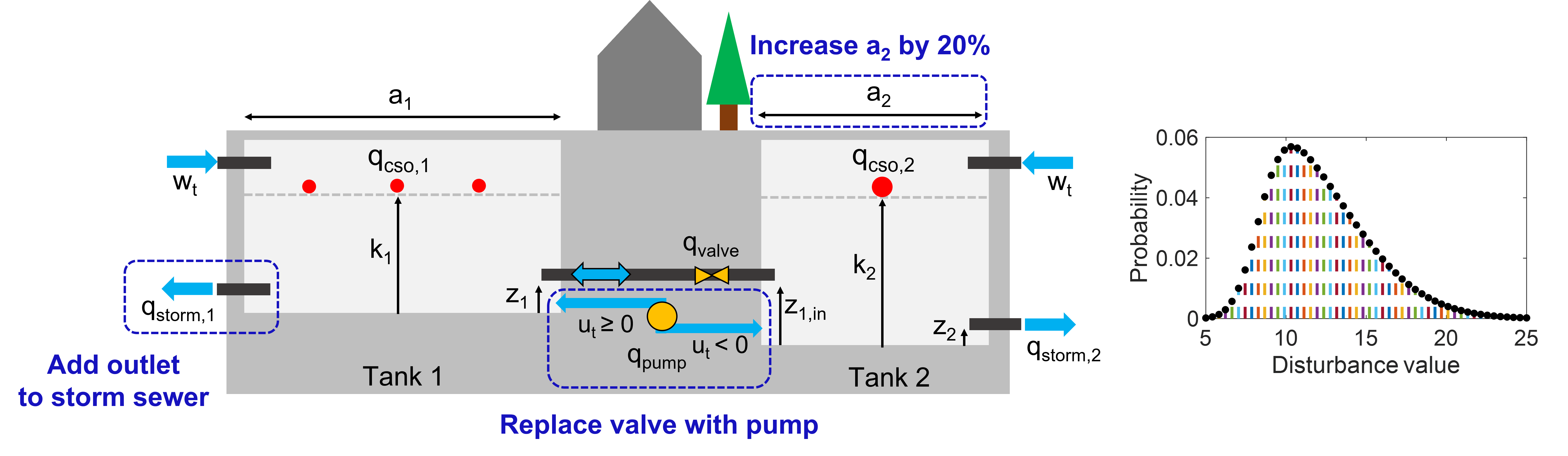
We consider the problem of modifying the design of an urban stormwater system (i.e., a network of pipes, storage tanks, natural streams, etc., near an urban area). Apart from being actively controlled, the stormwater system that we consider is otherwise typical.333Actively controlled stormwater systems are becoming more common but are relatively novel technologies, e.g., see [43]. The system consists of two tanks connected by a valve, and water flows by gravity between the tanks based on the relative difference in water levels and the position of the valve (Fig. 2). Water enters the system through a random process of surface runoff. Water exits the system through a storm sewer drain that is connected to tank 2 or through outlets that lead to a combined sewer. The storm sewer directs stormwater to a nearby water body; this is the desired outcome and occurs without penalty. Unfortunately, the storm sewer’s capacity is limited, and when water levels become too high, excess flows are directed to a combined sewer. In drier periods, a combined sewer carries a mixture of untreated wastewater and stormwater to a wastewater treatment plant. However, when storm events cause the flow in a combined sewer to exceed its design capacity, a flow regulator (downstream from our system) will divert some of the untreated mixture of stormwater and sewage into a nearby water body. This event is known as a combined sewer overflow. Combined sewers are present in older cities, such as Toronto and San Francisco, and overflows from these sewers can harm local ecosystems. We aim to use risk-averse safety analysis to examine how design modifications to the system above may reduce the risk of combined sewer overflows by managing the maximum water levels in the system.
5.2 System Model for the Baseline Design
The state is a vector of the random water levels in tank 1 and tank 2 at time . The co-domain of is ft2, where ft and is the maximum water level that tank can hold without releasing water into the combined sewer. The control input is the valve position at time , and the co-domain of is (closed to open, unitless). The tuple represents surface runoff that arises due to precipitation uncertainty. The disturbances are independent and identically distributed, and their distribution does not depend on the current state or control. The realizations of have units of cubic feet per second (cfs). The disturbance space is a subset of the non-negative orthant in containing finitely many elements, with . In prior work [44], we simulated a design storm in PCSWMM software (Computational Hydraulics International), which is an extension of the US Environmental Protection Agency’s Stormwater Management Model [45]. A design storm is a synthetic precipitation time series based on historical data that a local government uses to specify regulations for new or retrofitted stormwater systems. The empirical distribution from our simulations had positive skew, and the mean was approximately 12.2 cfs. We used these characteristics to inform the choice of the disturbance distribution shown in Fig. 2: mean (12.2 cfs), variance (9.9 cfs2), and skew (0.74).
Let be given. If , , and are the values of , , and , respectively, then the value of is given by
| (29a) | ||||
| such that if , then we redefine . The symbol is the duration between time and time , which is constant for all . In this model, for all . The function is chosen according to simplified Newtonian physics: | ||||
| (29b) | ||||
| Table 1 lists model parameters. The outlets to the combined sewer and to the storm sewer are equipped with outflow regulation devices that produce a linear outflow rate. For example, with is given by | ||||
| (29c) | ||||
where is tank 2’s maximum outflow rate to the storm sewer, is a discharge coefficient, , is gravitational acceleration, is the storm sewer outlet radius, and is the storm sewer outlet elevation. The outflow rates to the combined sewer, and , are defined similarly to (29c). The constraint set specifies the invert elevations of the combined sewer outlets (i.e., the maximum water levels that the tanks can hold without releasing water into the combined sewer). The function quantifies the maximum water elevation above the combined sewer invert elevations,
| (30) |
| Symbol | Description | Value |
| Surface area of tank 1 | 30000 ft2 | |
| Surface area of tank 2 | 10000 ft2 | |
| Discharge coefficient | 0.61 (no units) | |
| Acceleration due to gravity | 32.2 | |
| Minimum of (30) | 0 ft | |
| Maximum of (30) | 2 ft | |
| Combined sewer outlet elevation, tank 1 | 3 ft | |
| Combined sewer outlet elevation, tank 2 | 4 ft | |
| Maximum value of | 5 ft | |
| Maximum value of | 6 ft | |
| Length of discrete time horizon | 20 ( 1 h) | |
| Circle circumference-to-diameter ratio | 3.14 | |
| Storm sewer outlet radius | ft | |
| Valve radius | ft | |
| Duration of | 3 min | |
| Pipe elevation with respect to base of tank 1 | 1 ft | |
| Pipe elevation with respect to base of tank 2 | 2 ft | |
| Storm sewer outlet elevation | 1 ft | |
| N/A | Number of combined sewer outlets, tank 1 | 3 |
| N/A | Number of combined sewer outlets, tank 2 | 1 |
| N/A | Combined sewer outlet radius, tank 1 | 1/4 ft |
| N/A | Combined sewer outlet radius, tank 2 | 3/8 ft |
| ft feet, s seconds, min minutes, h hours. | ||
5.3 Verification of Assumption 1
It holds that for all , where is defined by (30). We choose for all . Thus, is -valued and continuous. The control space is compact. In our example, the stochastic kernel for the disturbance process does not depend on , which implies that it is constant and therefore continuous in . The dynamics function (29) is continuous because it is a composition of continuous functions. Recall that the function is continuous since .
5.4 Designs
We investigate the effect of different designs on the system’s safety, as quantified in terms of risk-averse safe sets. The designs are listed below:
-
a)
Baseline;
-
b)
Replace the valve with a controllable bidirectional pump, whose maximum pumping rate is ;
-
c)
Retrofit tank 1 with an outlet that drains to a storm sewer without penalty; or
-
d)
Increase the surface area of tank 2 by 20%.
We modify the baseline system model to obtain a model representing design b, c, or d. For design d, we set ft2. For design c, the equation for the flow through tank 1 changes to the following:
| (31) |
where takes the same form as in (29c).
For design b, the control space becomes , and the term is replaced by , which models the flow rate generated by a pump. Prior to presenting the form of , we introduce its dependencies, and . is a Boolean variable that determines whether the water level is too low to permit pumping, and the function represents a start-up phase. is true if and only if the pump attempts to push water from tank 1 to tank 2 (), but the water level in tank 1 is too low. has an analogous interpretation. Formally, we define and as follows:
| (32a) | ||||
| where is a threshold elevation and is a small positive number. We define the function as follows: | ||||
| (32b) | ||||
| We define as follows: | ||||
| (32c) | ||||
One can show that is a composition of continuous functions by replacing the case statements in (32c) with minimum and maximum operators:
Table 2 lists model parameters for the pump design (b).
| Symbol | Description | Value |
| Maximum pumping rate | 10 cfs | |
| Slack variable | ft | |
| Threshold pumping elevation | 1 ft | |
| ft feet, cfs cubic feet per second. | ||
5.5 Current Method vs. Under-approximation Method
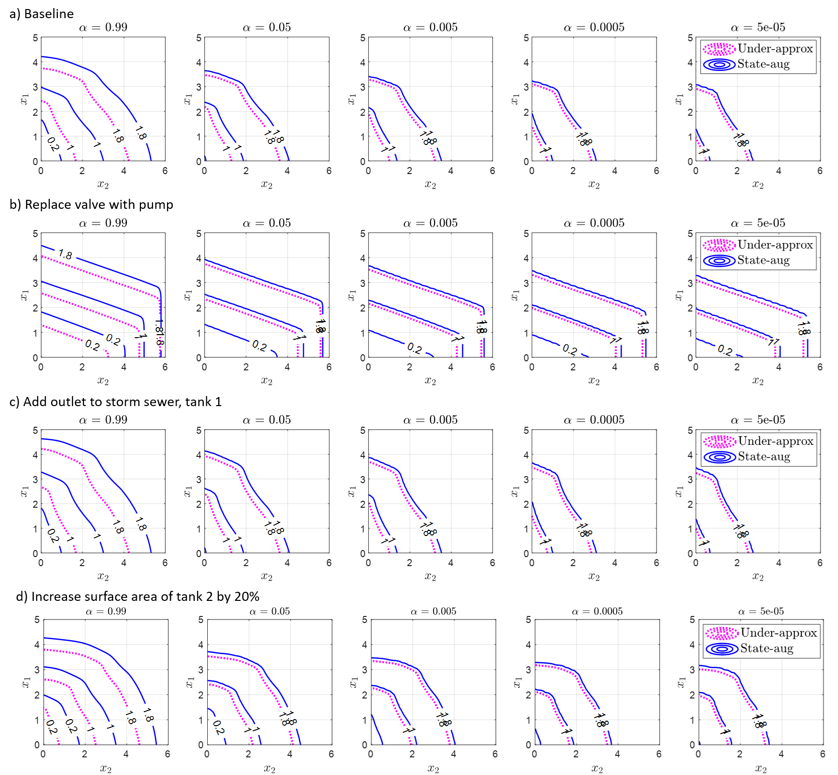
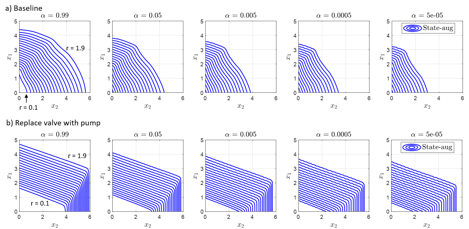
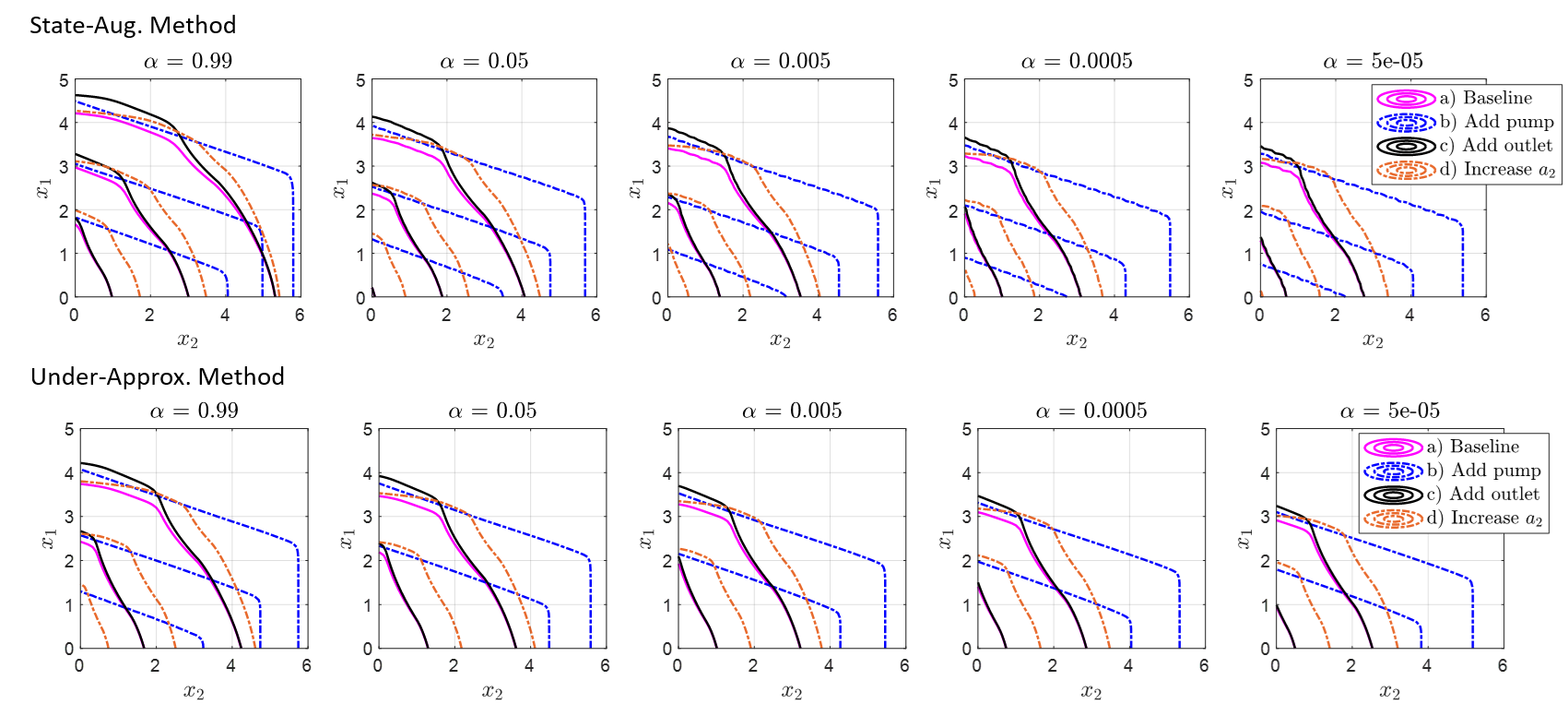
Computations of for the four designs are shown in Fig. 3. For comparison, we provide computations of the under-approximation set () using the method from our prior work [12]. The under-approximation method uses a -dependent soft-maximum and an -dependent upper bound for the CVaR to derive a -dependent upper bound for the optimal value (1) with . For a fixed , solving one MDP problem is required to compute for all and of interest. The DP iterates for this MDP problem are defined on the original state space , and the objective is an expected cumulative -dependent cost. We have explored values of between 10 and 120 in increments of roughly 10. We have chosen because this value provides relatively large estimates of for more risk-averse values of . The selection of an appropriate depends on one’s preferences, and additional guidance is provided in [12].
While no parameter tuning is required for the current method, which provides exactly in principle, greater computational resources are required. First, due to time inconsistency and a non-additive cost function, the dynamic program that determines the minimum CVaR is defined on an augmented state space, which is the Cartesian product of the original state space and the interval . Moreover, due to the definition for the CVaR (4), a second outer optimization with respect to the dual parameter is required. Consequently, the inner dynamic program is implemented repeatedly for different values of the dual parameter. While this increases the computational complexity significantly, problems with different dual parameters can be solved in parallel to reduce computation time.
One can run the under-approximation method on a standard laptop (2–4 CPU cores) in approximately 10 minutes for a fixed and a fixed design. However, this approach is not suitable for the current method. In particular, we used a high-performance computing cluster. The complete job (four designs) required about 54 hours and 30 CPU cores.444In the main paper, we state that about 13.5 hours is required for each design because (54 hours)/(4 designs) = 13.5 hours per design. We used the Tufts Linux Research Cluster (Medford, MA) running MATLAB (The Mathworks, Inc.), and our code is available from https://github.com/risk-sensitive-reachability/RSSAVSA-2021. These run-time and CPU values should be considered a rough comparison of the resources that naive implementations of the two methods require; we have made no attempt to optimize computational efficiency beyond parallelizing the operations in a given DP recursion. Table 3 summarizes the main trade-offs between the current method and under-approximation method.
| Current Method | Under-Approximation Method [12] |
|---|---|
| Provides exactly in principle | Provides an under-approximation for in principle |
| Does not require parameter tuning | The soft-maximum parameter requires tuning. |
| Requires significantly more computational resources | Requires significantly less computational resources |
| Useful for in-depth analysis of a small number of promising designs | Useful as a screening tool to identify more promising designs from a collection of candidate designs |
5.6 Discussion of the Numerical Results
We use the notation to indicate a computation of . This notation emphasizes the distinction between an exact mathematical quantity and a computation of this quantity returned by a computer program. The under-approximation method preserves interesting and potentially useful qualitative features that are provided by the current method. For example, the -contours for the pump design (b) are more rectangular in comparison to those for the baseline design (a) (Fig. 4). These features are apparent from the -contours as well (Fig. 3, first two rows, pink dotted lines). The -contours for the outlet design (c) are stretched along the -axis in comparison to the baseline design (a) (Fig. 5, top, black vs. pink). This effect is also seen by observing the associated contours of (Fig. 5, bottom, black vs. pink). Increasing the surface area of tank 2 (design d) stretches the contours of and along the -axis in comparison to the baseline design (Fig. 5, top and bottom, orange dotted vs. pink). As the risk-aversion level becomes smaller (more pessimistic), the contours of and contract, as we expect, while the qualitative features are preserved (Fig. 3).
While the under-approximation method recovers qualitative features and requires reduced computational resources, it tends to over-estimate the effect of making a design change (Table 4). Consequently, we see the under-approximation method as a preliminary screening tool to identify more promising designs from a collection of candidate designs. On the other hand, we see the current method as a tool for in-depth analysis of a small number of promising designs that have been selected a priori by preliminary screening.
The risk-aversion level allows one to specify a degree of pessimism in terms of a fraction of worst cases, which has benefits for designing systems in practice. Stormwater systems are often required to satisfy precise regulatory criteria. For example, an outflow rate must be no more than a given threshold when simulating the outcome from a (non-stochastic) design storm via hydrology and hydraulic modeling software, e.g., [45]. Our framework could be used in parallel with standard practices to quantify the effect of stochastic surface runoff on low-dimensional models of proposed designs, as the degree of risk aversion varies. The value of provides a systematic and interpretable way to assess a design with respect to varying degrees of pessimism about the future. While the typical minimax approach to control systems leads to robust designs by adopting a worst-case perspective, designing for the worst case may not be financially feasible, especially given the limited budgets afforded to “ordinary” rather than “safety-critical” infrastructure. Therefore, the flexibility afforded by may be useful for assessing trade-offs between system performance and financial considerations in practice.
| 0.99 | b vs. a | c vs. a | d vs. a |
| Current Method | 0.93 | 0.079 | 0.34 |
| Under-approximation Method | 2.6 | 0.069 | 0.93 |
| 0.05 | b vs. a | c vs. a | d vs. a |
| Current Method | 2.1 | 0.068 | 0.71 |
| Under-approximation Method | 3.6 | 0.059 | 1.3 |
| 0.005 | b vs. a | c vs. a | d vs. a |
| Current Method | 3.1 | 0.059 | 1.1 |
| Under-approximation Method | 5.1 | 0.072 | 1.9 |
| 0.0005 | b vs. a | c vs. a | d vs. a |
| Current Method | 4.9 | 0.055 | 1.8 |
| Under-approximation Method | 7.6 | 0.03 | 2.8 |
| 0.00005 | b vs. a | c vs. a | d vs. a |
| Current Method | 9.0 | 0.054 | 3.3 |
| Under-approximation Method | 14 | 0.031 | 5.3 |
| We list the increase in the size of a risk-averse safe set for design b, c, or d compared to the baseline (design a). This is a quantitative depiction of the some of the results in Fig. 5. Let denote the number of states in the computation of for design y and . Let denote the number of states in the computation of for design y, , and . Each quantity in a row labeled Current Method takes the form . Each quantity in a row labeled Under-approximation Method takes the form . | |||
6 Conclusions
By overcoming theoretical challenges attributed to optimizing the CVaR of a trajectory-wise maximum cost, we have shown that risk-averse safe sets enjoy an equivalent representation in terms of the solutions to a family of stochastic dynamic programs. We are investigating extensions to higher-dimensional systems in the finite-time case using extreme value theory [31] and in the infinite-time case using value function approximations. In the future, we hope to study new problems that combine performance and risk-averse safety criteria, such as optimizing a utility functional subject to a constraint on the CVaR of a maximum cost.
7 Appendix
Here, we provide step-by-step technical details underlying the theoretical results of the main paper. Throughout the Appendix, we assume that Assumption 1 holds, even if this is not explicitly stated. This assumption is useful for ensuring that integrals are well-defined, optimal policies exist, etc. In particular, while a milder assumption may be sufficient, we construct using Assumption 1 (Sec. 7.3).
7.1 An Extended Proof for Lemma 1
Lemma 1 (Existence of a minimizer in ): Let Assumption 1 hold. Let and be given. Suppose that is measurable relative to and , and suppose that for every . Define with (8). Then,
| (33) |
where min means that a minimizer exists.
Proof 7.7.
Note that is given by
| (34) | ||||
| (35) |
is -valued in particular because
| (36) |
Define
| (37) |
is finite because
| (38) |
To derive the second inequality, note that
| (39) |
We will show that for any , , from which we will conclude that
| (40) |
First, for any , holds by the definition of . Second, consider , equivalently, . In this case, for every ,
| (41) |
and therefore,
| (42) |
We continue the algebra to find that
| (43) |
If in (43), then we have
| (44) |
Now, since and , it holds that
| (45) |
Therefore,
| (46) |
The third and last case is to consider , equivalently, , from which we deduce that for every ,
| (47) |
It follows that
| (48) |
We have shown that for every , holds, and therefore, we conclude that (40) holds, equivalently,
| (49) |
To show that , we prove that is continuous in .555The infimum of a lower semi-continuous function on a compact topological space is attained [42, Th. A6.3, p. 389]. Since , it suffices to show that
| (50) |
is continuous in . We will show that for any and ,
| (51) |
that is, is Lipschitz continuous in with Lipschitz constant equal to one. First, note that for any and , we have
| (52) |
because
| (53) |
is non-decreasing, and thus,
| (54) |
where the equality holds because . In addition, holds because
| (55) |
By using (52) and , we have that for any ,
| (56) | ||||
| (57) | ||||
| (58) |
From (58), we conclude that for any ,
| (59) |
By taking the infimum over , we have
| (60) |
and by using the definition (50), it holds that
| (61) |
By exchanging the roles of and in (56)–(61), we find that
| (62) |
| (63) |
which proves the desired statement (51).
7.2 About the Dirac measure
This subsection derives a fact about the Dirac measure. While the content is elementary, we could not find a full explanation in any classical measure theory or real analysis textbook. So, we provide an explanation here.
Let us study a Dirac measure on a Borel space. Suppose that is a Borel space and is given. Let be the Dirac measure in concentrated at . is also called the unit mass concentrated at [39, p. 17]. If is Borel-measurable, then
| (64) |
Why does the equation (64) hold? Recall that is defined by [39, Examples 1.20 (b), p. 17], [32, p. 130 top],
| (65) |
and therefore,
| (66) |
for every . First, suppose that , where . In this case, we have
| (67) |
where holds by the definition of the integral [42, 1.5.3, p. 36]. Second, suppose that , where , is a disjoint collection of sets in , and for every . In this second case, is called a nonnegative finite-valued simple function, and we have
| (68) |
Third, suppose that is a nonnegative Borel-measurable function. Then, is the (pointwise) limit of a nondecreasing sequence of nonnegative, finite-valued, simple functions [42, Th. 1.5.5 (a), p. 38]. That is, is nonnegative, finite-valued, and simple for every , for every , and
| (69) |
Then, by the Monotone Convergence Theorem [42, 1.6.2, p. 44], we have
| (70) |
Moreover, since is nonnegative, finite-valued, and simple, we have
| (71) |
All together, we have
| (72) |
Finally, suppose that is an arbitrary Borel-measurable function. Then, we can write in terms of its positive and negative parts as follows [42, p. 37]:
| (73) |
The right side of (73) can never have the form because
-
•
and ;
-
•
and ;
-
•
and .
Since and are Borel-measurable and nonnegative, we have
| (74) | ||||
Then,
| (75) |
does not have the form , as explained above. Lastly, we apply the definition of the integral [42, p. 37] to conclude that
| (76) |
which shows the desired statement (64). In the next subsection, we derive and the associated expectation.
7.3 A Derivation for and the Associated Expectation
It is well-established that the system model of interest permits the construction of a unique probability measure on a space containing all possible trajectories.666For example, see [32, Prop. 7.28, pp. 140–141], which is a special case of the Ionescu-Tulcea Theorem. This measure is used to evaluate expectations of random variables, which can represent costs that may be incurred as the system evolves over time. Recall Assumption 1:
-
1.
There exist and such that for every . (We define .)
-
2.
The control space is compact.
-
3.
For every , and are continuous functions, and is a continuous stochastic kernel.
Note that we are working with Borel spaces:
-
•
, , and are Borel spaces by the assumed system model. is a closed subset of , which implies that . Since is a Borel space and , is also a Borel space [32, Prop. 7.12, p. 119]. with the product topology is a Borel space because it is a finite Cartesian product of Borel spaces [32, Prop. 7.13, p. 119]. Similarly, with the product topology is a Borel space. Borel spaces are separable and metrizable [32, p. 118].
Often, we use the notation , and or denotes an arbitrary element of . If is a metrizable space, we equip the set of probability measures on with the weak topology, and we denote this topological space by [32, p. 122, p. 127]. Next, we will define a stochastic kernel on given that provides the conditional distribution for the realizations of the augmented state.
7.3.1 Construction and Analysis of
Recall the definition
| (77) |
and the notation
| (78) |
For every , let be the product measure of and . The product measure is the unique measure on such that
| (79) |
by [42, Cor. 2.6.3, p. 100] and [32, Prop. 7.13, p. 119]. When we apply [42, Cor. 2.6.3], we are working with the probability spaces and , where the measures are sigma finite because they are finite (as they are probability measures). The domain of the product measure is the product sigma algebra of and [42, Cor. 2.6.3], which is the smallest sigma algebra that contains all sets of the form with and [42, p. 97]. Since and are Borel spaces, the product sigma algebra of and is equivalent to [32, Prop. 7.13, p. 119].
Lemma 7.8 (Analysis of ).
Under Assumption 1, is a continuous stochastic kernel on given .
Proof 7.9.
For every , we have that because is a probability measure on and we have equipped the set of probability measures on with the weak topology. is a stochastic kernel on given because it provides a family of elements of , where each element of depends on an element of [32, Def. 7.12, p. 134]. Now, consider the function defined by
| (80) |
To show that is a continuous stochastic kernel, we need to show that is continuous [32, Def. 7.12]. Recall the following properties:
-
•
The map defined by
(81) is continuous because is continuous, , , and are Borel spaces, and is a continuous stochastic kernel on given [32, top of p. 209].
-
•
The map defined by
(82) is continuous. The reason is three-fold: the map defined by is continuous [32, Cor. 7.21.1, p. 130],777In our work, denotes the Dirac measure on concentrated at . The reference [32] uses the notation instead. When reading [32, Cor. 7.21.1, p. 130], note that a homeomorphism is continuous. the map is continuous due to and being continuous, and a composition of two continuous maps on topological spaces is continuous [36, p. 119].
- •
-
•
We paraphrase the following result [32, Lemma 7.12, p. 144]: If and are separable metrizable spaces, then the map defined by
(84) where is the product of the measures and , is continuous.
Since and are Borel spaces, they are separable and metrizable [32, p. 118]. For every , the product of and is , and thus,
| (85) |
All together, we have
| (86) |
Since is a composition of continuous maps, is continuous. We conclude that is a continuous stochastic kernel under Assumption 1.
7.3.2 Construction of and Definition of
Let Assumption 1 hold, and let and be given. Please note the following items:
-
•
is the Dirac measure on concentrated at the point , i.e., for every ,
(87) - •
-
•
For every , is a Borel-measurable stochastic kernel on given by the definition of .
Next, we use [32, Prop. 7.28] to construct a unique probability measure , where we define . We translate the notation from [32, Prop. 7.28] to our setting in Tables 5 and 6. The text in blue denotes the symbols from [32, Prop. 7.28], and the text in black denotes our symbols.
| Borel space | ||||||||
| Borel space | ||||||||
| Sample | ||||||||
| Sample |
| Stochastic kernel or probability measure | Samples permitted in conditional statement, | Stochastic kernel or probability measure |
|---|---|---|
| N/A | ||
The result [32, Prop. 7.28], which is a special case of the Ionescu-Tulcea Theorem, states that for , there is a unique probability measure such that
| (88) | ||||
for every , , . Using and the notation from Tables 5 and 6,888The tuple has entries. there is a unique probability measure such that
| (89) | ||||
for every and for every . While depends on , we do not include when writing the symbol for brevity.
Let be measurable relative to and , i.e., . Our presentation of the definition of the expectation of with respect to follows [42] and [32]. The positive and negative parts of are defined by
| (90) | ||||
| (91) |
respectively, where and are measurable relative to and [42, p. 37], [32, p. 103]. The expectation of with respect to is defined by
| (92a) | |||
| if the right side of (92a) does not take the form ; if the right side of (92a) takes the form , then we say that does not exist [42, p. 37]. While depends on through , we do not include when writing the symbol for brevity. If or , that is, if exists,999If is Borel-measurable and nonnegative, then for every , which implies that . then we have | |||
| (92b) | |||
by [32, Prop. 7.28, see Eq. (47)], where we only write some of the stochastic kernels from (89) for brevity. Many of the subsequent sections will use the definition of the expectation with respect to .
7.3.3 Further Discussion about Integration
Suppose that is Borel-measurable (i.e., measurable relative to and ) and bounded below. Let be given. Consider the function defined by
| (93) |
where we only write some of the integrals for brevity. Why is (93) Borel-measurable and bounded below? To address this question, the following fact is useful.
Remark 7.10 (Extending stochastic kernels).
Suppose that , , and are Borel spaces, and let be a Borel-measurable stochastic kernel on given . Then, the stochastic kernel on given defined by
| (94) |
is Borel-measurable. To prove this fact, we need to show that the function defined by
| (95) |
is Borel-measurable, i.e., for every , it holds that
| (96) |
Let be given. Since is a Borel-measurable stochastic kernel on given , the function defined by
| (97) |
is Borel-measurable, implying that
| (98) |
Since contains all sets of the form with and (for instance, see the proof of [32, Prop. 7.13, p. 119]), we have
| (99) |
By (94), (95), and (97), we have
| (100) |
Therefore,
| (101) |
which is a member of by (99).
The desired properties of (93) (Borel-measurable, bounded below) follow from Remark 7.10 and by successive applications of [32, Prop. 7.29, p. 144], which we paraphrase: Let and be Borel spaces, be a Borel-measurable stochastic kernel on given , and be Borel-measurable and bounded below. Then, the function defined by is Borel-measurable and bounded below.101010The bounded-below property is not included in the statement of [32, Prop. 7.29, p. 144]. To show that (93) is Borel-measurable and bounded below, one applies this proposition to the inner-most integral in (93) and then proceeds to the outer-most integral. We outline the first two steps below:
-
1.
Consider and . Define a stochastic kernel on given by
(102) for every . is Borel-measurable due to the Borel-measurability of (Remark 7.10). The function in (93) is Borel-measurable and bounded below by assumption. Thus, the function defined by
(103) is Borel-measurable and bounded below by applying [32, Prop. 7.29, p. 144]. We also use the fact that a finite Cartesian product of Borel spaces with the product topology is a Borel space [32, Prop. 7.13, p. 119].
- 2.
7.4 More Measure-theoretic Fundamentals
First, we recall some preliminaries. Every takes the form
| (105) |
and we recall the notation . We define , , and to be projections from to , , and , respectively, such that for every of the form in (105),
| (106a) | ||||
| (106b) | ||||
| (106c) | ||||
depends on , , and as follows:
| (107) |
The realizations of are concentrated at , where can be any element of . For every and , we define
| (108) | ||||
| (109) | ||||
| (110) |
where is defined by
| (111) |
which is nonnegative and continuous.
Remark 7.11 (Equivalent expressions for and ).
7.4.1 Analysis of
Here, we explain why is a random object. First, we introduce some terminology. If and are measurable spaces and is measurable relative to and , then is called a random object [42, p. 214]. If , then is called a random variable. If , then is called an extended random variable.
Now, let be given, and recall that and are defined by
| (115) | |||
| (116) |
for every of the form in (105). is measurable relative to and ; i.e., is Borel-measurable. This is because for every , we have
| (117) | ||||
| (118) | ||||
| (119) |
The set is an element of because is a measurable rectangle by (119); e.g., see the proof of [32, Prop. 7.13, p. 119]. Analogous steps show that is measurable relative to and ; i.e., is Borel-measurable.
To show that is Borel-measurable, we can use [32, Prop. 7.14, p. 120], which we paraphrase: Let , , and be Borel spaces, and for , let be a function. If and are Borel-measurable, then the function defined by
| (120) |
is Borel-measurable.
In our problem, , , and are Borel spaces, and and are functions. For brevity, we define . Since and are Borel-measurable, the function defined by
| (121) |
is Borel-measurable, i.e., measurable relative to and , by [32, Prop. 7.14]. The function being Borel-measurable means that is a random object.
7.4.2 Studying and
The next lemma provides a relationship between and .
Lemma 7.12.
Let Assumption 1 hold, and let , , and be given. Then, we have
| (122) |
Proof 7.13.
is a random variable on because is measurable relative to and , and is a probability measure on . For convenience, we restate (109) using
| (123) |
and using the definition of (111) and the definition of (108):
| (124) |
By comparing (123) and (124), to show that , it suffices to show that
| (125) |
Indeed, if (125) holds, then
| (126) |
equivalently, using (123),
| (127) |
equivalently, using (124),
| (128) |
The statement (128) implies that
| (129) |
which is equivalent to the desired statement (122). The integrals in (129) exist because and are Borel-measurable and nonnegative. Thus, it suffices to show (125) to complete the proof.
We need to explain two items before proceeding. The first item concerns the probability measure induced by . This measure is defined by
| (130) |
It holds that . Indeed, for every , we have
| (131) | ||||
because the innermost integrals evaluate to one. Secondly, since the stage and terminal cost functions are bounded below by , we have
| (132) |
for every and for every . That is, the is redundant for evaluating the maximum. To see this explicitly, denote for brevity. If
| (133) |
then
| (134) |
which is equivalent to (132) because
| (135) |
The inequality (133) holds because and .
Now, suppose that satisfies . Then,
| (136) | ||||
| (137) | ||||
| (138) | ||||
| (139) | ||||
| (140) |
Therefore,
| (141) |
is a subset of
| (142) |
and hence,
| (143) |
The statement that we desire is (125), which is the same as . It suffices to show that , since then we would have
| (144) |
Finally, we have
| (145) | ||||
| (146) | ||||
| (147) | ||||
| (148) | ||||
| (149) |
where the last line holds because (87).
7.4.3 Analysis of
We recall from (109)–(110) that for every and ,
where is a nonnegative continuous function defined by . Each is real-valued and Borel-measurable, and , , and are Borel-measurable functions (106). As Borel-measurability is preserved under compositions and maximums, for every is Borel-measurable, i.e., measurable relative to and . The following lemma verifies additional useful properties.
Lemma 7.14.
Let Assumption 1 hold. For every , , , and , is an extended random variable on . In addition, for every , it holds that .
Proof 7.15.
Let and be given. For every and , is a probability space because is a sigma algebra of subsets of and is a probability measure on . To verify that is an extended random variable on , we must show that is measurable relative to and .
For every , it holds that , so we can view as a function from to . Next, we explain why is measurable relative to and .
-
1.
Note that is generated by, for example, the family [36, p. 45].
-
2.
Since is generated by , is measurable relative to and if and only if
(150) by [36, Prop. 2.1, p. 43].
-
3.
Let be given. So, for some . Then,
(151) where the last step holds because for every .
-
4.
Since is an open set in , it is an element of . Since and is measurable relative to and , we have that
(152) proving (150). We conclude that is measurable relative to and .
The last part of the proof is to show that . We will use the following: for any with ,
| (153) | ||||
| (154) |
and
| (155) |
To show that for every , first let be given. For every , we have
| (156) | ||||
| (157) | ||||
| (158) | ||||
| (159) | ||||
| (160) |
Now, let . For every , we have
| (161) | ||||
| (162) | ||||
| (163) | ||||
| (164) |
Therefore, we conclude that for every .
7.4.4 Change-of-Variable Image Measure Theorem
We paraphrase a change-of-variable image measure theorem from [42, Th. 1.6.12, p. 50]: Let and be measurable spaces, and let be measurable relative to and . Suppose that is a measure on . Define a measure on by
| (165) |
If is measurable relative to and and , then
| (166) |
in the sense that if one of the integrals exists, then the other integral exists also, and the two integrals are equal. Some textbooks, e.g., [37, p. 92], call (165) the image measure of by .
7.4.5 Relating Integrals with respect to and
Let and be given. Recall the notation , where is an arbitrary element of . For every , the probability measure on induced by encodes the process starting from time zero and ending where may be realized. The symbol denotes this induced measure. While depends on , , , and , we omit the symbol from the notation for brevity. Recall that (121) is defined by
For any , it holds that
| (167) |
because is measurable relative to and (Sec. 7.4.1). Thus, we can use the probability measure (89) to evaluate the event . This evaluation defines the induced probability measure :111111Since we only know the form of on measurable rectangles in , we only know the form of on measurable rectangles in . We note that (168) A set of form is called a measurable rectangle in . contains measurable rectangles and other forms of subsets of .
| (169) |
We recall from (131) that . Note that
| (170) |
Let be given, and suppose that is measurable relative to and . We note the following properties:
-
•
and are measurable spaces;
-
•
is measurable relative to and (Sec. 7.4.1);
-
•
(89) is a probability measure on ;
-
•
(169) is a probability measure on .
Therefore, by the change-of-variable image measure theorem (Sec. 7.4.4), we have
| (171) |
in the sense that if one of the integrals exists, then the other integral exists as well, and the two integrals are equal. We would like to provide an explicit form for (171).
We consider the case for and the case for separately. First, if , then
| (172a) | |||
| We are permitted to apply (64) because is Borel-measurable and (with the product topology) is a Borel space. In the second step, we use (131). | |||
Now, let be given, and suppose that or exists.121212If exists, then exists and by the statement below (171). Similarly, if exists, then exists and by the statement below (171). Then, we have
| (172b) |
Next, we explain why the last line of (7.4.5) holds. The key idea is to use the change-of-variable image measure theorem (Sec. 7.4.4) again but for a different reference measure (to be denoted by ). For convenience, we define
| (173) |
is a finite sequence of Borel spaces, (173) is a Cartesian product of these spaces, is given, is a continuous stochastic kernel under Assumption 1 (Lemma 7.8), and is a Borel-measurable stochastic kernel. Hence, we apply [32, Prop. 7.28, pp. 140–141] to guarantee the existence of a unique probability measure (which depends on as well) such that
| (174) |
for every , and if is Borel-measurable and exists, then
| (175) |
We define by
| (176) |
and therefore, for every , it holds that
| (177) | ||||
We know that the set because this set is a measurable rectangle. We claim that
| (178) |
Indeed, for every , we have131313We use the product measure instead of the two measures and separately. If we did not use the product measure, then the expression would arise in (179). This expression does not quite make sense because need not take the form with and .
| (179) | ||||
The third step of (179) holds because we use (89) and the innermost integrals evaluate to one. Now, we apply the change-of-variable image measure theorem [42, Th. 1.6.12, p. 50]. is defined by (176). It is Borel-measurable, and hence, we write . By our previous discussion, we have and for every . By [42, Th. 1.6.12, p. 50], if and , then
| (180) |
in the sense that if one of the integrals exist, then the other does as well, and the two integrals are equal. Now, consider and , and recall our assumption that or exists.
-
•
exists exists and the two integrals are equal (Footnote 12).
-
•
and .
-
•
and exists exists.
Therefore, we have
| (181) |
and the integrals exist. Since is Borel-measurable and (181) exists, we have
| (182) | ||||
Finally, we have
| (183) | ||||
completing the proof of the last line of (7.4.5) under the assumption that or exists.
7.5 An Extended Proof for Theorem 1
For every , we denote a conditional expectation of given by such that
| (184) |
which is unique almost everywhere with respect to . Next, we study in Theorem 1.
Theorem 1 (Properties of ): Let , , and be given, and let Assumption 1 hold. Define the function by141414 and is defined by (185) for every , for every , . Hence, we can view as a function from to .
| (185) |
Then, the following relations hold:
| (186) | ||||
| (187) | ||||
| (188) |
Proof 7.16.
We note the following facts. For every ,
-
•
is an extended random variable on (Sec. 7.4.3);
-
•
is a random object, as it is measurable relative to and (Sec. 7.4.1);151515The following statements are equivalent: is measurable relative to and ; is Borel-measurable; and .
-
•
exists (it does not take the form ) because for every .
Therefore, by [42, Th. 6.3.3, p. 245], there is a function , measurable relative to and , such that for every ,
| (189a) | |||
| We define | |||
| (189b) | |||
which is unique almost everywhere with respect to [42, Th. 6.3.3]. This result holds as a consequence of the Radon-Nikodym Theorem.
First, we write (189) in a particularly useful form. Let be given. Consider in (189) to find that
| (190) |
Since exists, it follows that (190) exists. Since is measurable relative to and and exists, we apply the change-of-variable image measure theorem to find that
| (191) |
where the integrals exist. By combining the previous two expressions (190)–(191), we have
| (192) |
We note that (192) holds for every because it has been derived for an arbitrary time index .
Next, we show (188), i.e.,
Let be given. From Lemma 7.14, we have , and therefore,
| (193) |
where the integrals exist because is nonnegative and Borel-measurable for every . Since , it holds that . Since (192) applies to any time index in , we have
| (194) |
We show (188) by combining prior steps:
| (195) |
noting that is arbitrary.
The next result is useful for Theorem 2.
7.6 Analysis of Lower Semi-continuous Bounded Below Functions
Variations of the lemma in this section can be found in the literature, e.g., see [32, Lemma 7.14 (a), p. 147] and [42, Th. A6.6, pp. 390–391].161616Another example is [41, Prop. D.5, pp. 182–183]. Our proof combines techniques from these textbooks. We present the technical details of the proof in one place for convenience. The notation denotes the Banach space of bounded, real-valued, and continuous functions on , where is a metrizable space.
Lemma 7.17.
Let be a metrizable space. Suppose that is lower semi-continuous (l.s.c.) and bounded below by zero. Then, there is a sequence in such that , i.e.,
-
1.
for every and , and
-
2.
for every .
Remark 7.18 (Generalization of Lemma 7.17).
Before proving the lemma, we note a generalization. Let be l.s.c. and bounded below by . We would like to show that there is a sequence in such that . Define , which is l.s.c. and bounded below by 0. By Lemma 7.17, there is a sequence in such that . Now, define . Then, is a sequence in such that , which is equivalent to .
A proof for Lemma 7.17 follows.
Proof 7.19.
Let be a metric on . We recall that is l.s.c. for any sequence in converging to ,171717 as . it holds that .
There are two cases to consider. The first case is that for every .181818We know that for every because is bounded below. In this case, we define by
| (203) |
which implies that
| (204) |
because for every . For every , is constant and finite, and therefore is continuous and bounded, i.e., . Finally,
| (205) |
which completes the proof in the first case.
Now, in the second case, there exists an such that . Define
| (206) |
Since for every and , and since for every , we have
| (207) |
Thus, zero is a lower bound for the set for every and , which implies
| (208) |
Since , , and metrics are real-valued, we have
| (209) |
Thus, for every and . (In (209), for example, we have written “,” which means for every and for every . In the rest of the proof, we use the symbol .)
To show that for every , note that since for every and for every , we have
| (210) |
By taking infima over , we obtain
| (211) |
To show that , note that
| (212) |
which we obtained by setting in the objective of .
For any , is an increasing sequence that is bounded above by . Thus, the limit of exists in (it may be ), and the limit is less than or equal to . Therefore,
| (214) |
For any , to show that is (uniformly) continuous (with respect to ), we will show that
Using the procedure on p. 126 of [32] (a symmetry argument using the definition of ), we have that
| (215) |
Let be given, and set . Suppose that satisfies . Then, we have
| (216) |
Thus, for every , is (uniformly) continuous (with respect to ).
We will show that (214) holds with equality by considering two cases. In the first case, we assume that is finite-valued. Let be given. For every , , which implies (by using the definition of the infimum) that
| (217) |
Note that depends on and , which we do not write explicitly for brevity. We will construct a sequence using (217). Let be given. Since , we have
| (218) |
Since , we have
| (219) |
By repeating this process, we obtain a sequence in such that
| (220) |
Moreover, since and for every , we have
| (221) |
Therefore,
| (222) |
where we also use the fact that for every . Since is positive and finite,
| (223) |
Since is finite, it follows that
| (224) |
The statements (223) and (224) imply that the limit of exists and equals zero. This is because
| (225) |
and
| (226) |
and therefore,
| (227) |
which allows us to conclude that
| (228) |
Moreover, since is lower semi-continuous and by (228), we have
| (229) |
By using (220), , and , we have
| (230) |
which implies that
| (231) |
By (229), (231), and the existence of the limit of , we have
| (232) |
Since , it follows that
| (233) |
Since the above analysis holds for any , we conclude that
| (234) |
Since the above analysis holds for any , we have that for every , under the assumption that is finite-valued.
Now, suppose that is not necessarily finite-valued. The function defined by is increasing and continuous (Fig. 6). The inverse of exists and is increasing and continuous; the inverse is such that (Fig. 6). Since the range of is , the composition is finite-valued and bounded below by 0.
As a consequence of being increasing, continuous, and finite-valued, and being l.s.c., the composition is also l.s.c. To show this explicitly, let converge to , i.e., , and we will show that
| (235) |
Since converges to and is l.s.c., it holds that
| (236) |
Since is increasing and its domain is , we have
| (237) |
Now,
| (238) |
The second inequality holds because
| (239) |
By (238) and since is continuous,
| (240) |
Let be given. Note that
| (241) |
and since is increasing, it holds that
| (242) |
Now, is a lower bound for , and so it is less than the greatest lower bound,
| (243) |
Since we have derived (243) for any , it holds for every ,
| (244) |
The limit of the left side is the limit inferior, and the limit of the right side exists by (240), and thus,
| (245) |
Finally, we derive
| (246) |
which shows that is lower semi-continuous.
Since is finite-valued, l.s.c., and bounded below by 0, there is a sequence of continuous functions such that
-
1.
for every and ,191919Recall that is bounded above by . and
-
2.
for every .
Recall that such that is continuous and increasing (Fig. 6). It follows that
-
1.
for every and , and
-
2.
for every .
In summary, is continuous and .
For any , we define by
| (247) |
which is a composition of continuous functions, and therefore is continuous. Each is bounded because
| (248) |
It holds that
| (249) |
holds because
| (250) | ||||
| (251) |
and therefore,
| (252) |
holds because
| (253) |
Finally, since is continuous, we have for every ,
| (254) |
The last equality holds because
| (255) |
In summary, each is continuous and bounded and , where need not be finite-valued. This concludes the proof of Lemma 7.17.
We will use Lemma 7.17 to show that key properties are preserved under integration, which is needed for Theorem 2.
7.7 Analysis of Properties under Integration
Recall the notation and . We consider the following conditions:
-
1.
For every , and are continuous functions, and is a continuous stochastic kernel on given ;
-
2.
For every , , where and .
Lemma 7.20.
Let Conditions (i)–(ii) hold. If is lower semi-continuous (l.s.c.) and bounded below by zero, then the function defined by
| (256) |
is l.s.c. and bounded below by zero.
Lemma 7.20 is different from [32, Prop. 7.31, p. 148] because the functions , , and appear in the integral in (256). Therefore, we cannot say that Lemma 7.20 holds by this proposition immediately. To prove Lemma 7.20, we use Lemma 7.17 from the previous subsection and two other results, which are stated below.
Lemma 7.21.
Let Conditions (i)–(ii) hold. If , then the function defined by (256) is continuous.
Lemma 7.22.
Let Conditions (i)–(ii) hold. Let be Borel-measurable for every , be Borel-measurable, and . Suppose that holds, i.e., for every and for every . Then, for every , we have
| (257) |
In short, Lemma 7.22 holds by an application of the Monotone Convergence Theorem [42, Th. 1.6.7, p. 47].
First, we prove Lemma 7.20, and then we prove the supporting results.
Proof 7.23.
Since for every , we have
| (258) |
For every , it holds that
-
1.
is Borel-measurable,
-
2.
is nonnegative, and
-
3.
is a probability space.
By the above three items, the integral
| (259) |
exists and is nonnegative for every . Therefore, is bounded below by zero.
To prove that is l.s.c., it suffices to show that if is a sequence in converging to , then
| (260) |
is a metrizable space,202020 is a metrizable space because and are Borel spaces, a Cartesian product of Borel spaces with the product topology is a Borel space, and a Borel space is metrizable [32, pp. 118–119, Prop. 7.13]. and is l.s.c. and bounded below by zero by assumption. Therefore, by Lemma 7.17, there is a sequence in such that , i.e.,
-
1.
for every , and
-
2.
for every .
Let and be given, and consider a probability space . Since , we have
| (261) |
Since , , , and are Borel-measurable functions, the functions
| (262) | ||||
are also Borel-measurable. It follows that
| (263) | ||||
where all the integrals exist. Since the inequality (263) was derived for arbitrary and , we have
| (264) |
For any , we have , which implies that is continuous (Lemma 7.21). Therefore, we have
| (265) |
where we use .
7.7.1 Proof of Lemma 7.21
Recall that and are continuous functions, and is a continuous stochastic kernel. We will show that if , then the function defined by (256) and provided below:
is continuous by applying [32, Prop. 7.30, p. 145] to our problem setting.
Proof 7.24.
The spaces , , and are separable and metrizable.212121, , and are Borel spaces, and therefore, they are separable and metrizable [32, p. 118]. is a closed set in is a Borel space. , , and are Borel spaces by the assumed system model. A countable Cartesian product of Borel spaces with the product topology is a Borel space [32, Prop. 7.13, p. 119]. is a continuous stochastic kernel on given by assumption. Recall that is the space of probability measures on with the weak topology. The following statements are equivalent:
-
1.
is a continuous stochastic kernel on given .
-
2.
The function defined by is continuous [32, Def. 7.12, p. 134].
-
3.
For any converging to , it holds that converges to in the weak topology.
-
4.
For any , it holds that for any continuous bounded function , i.e., [32, Prop. 7.21, p. 128].
The stochastic kernel on given defined by
| (268) |
is continuous. To see this, let and a continuous bounded function be given. Then,
| (269) |
where the equalities hold by (268); the limit holds because is a continuous stochastic kernel on given , , and is continuous and bounded.
If , then the function defined by
| (270) |
is continuous by [32, Prop. 7.30]. Hence, it suffices to show that
| (271) |
satisfies . Consider the function
| (272) | ||||
| (273) |
Since , , and are continuous, it holds that
| (274) | ||||
| (275) | ||||
| (276) |
for any sequence in converging to a point . Therefore, is continuous. The function can be written as , where denotes composition. Since the composition of continuous functions is again a continuous function [sutherland1975introduction, Prop. 3.1.8], is continuous. Moreover, it holds that
| (277) |
where the last inequality holds because is bounded. Hence, is bounded. Since is continuous and bounded, we have that , which concludes the proof of Lemma 7.21.
7.7.2 Proof of Lemma 7.22
Recall that and are continuous functions, and is a continuous stochastic kernel. Let be Borel-measurable for every , be Borel-measurable, and . Suppose that holds, i.e., and for every . Under these conditions, we will show that for every
| (278) |
Proof 7.25.
We use the Extended Monotone Convergence Theorem [42, Th. 1.6.7, p. 47]: Let be a measure space. Let be functions from to , which are measurable relative to and . If for every and , , and ,222222 means for every and , and for every . then .
Let be given. We use the probability space . Define the functions for every , , and as follows:
| (279) | ||||
| (280) | ||||
| (281) |
The functions (279)–(281) are measurable relative to and . , , , and are continuous, which implies that they are Borel-measurable. and are Borel-measurable, and the composition of Borel-measurable functions is Borel-measurable.
Recall that for every and . Therefore, for every and , we have
| (282) |
Recall that for every , we have . Let be given. Then, and . Therefore,
| (283) |
Since in (283) is arbitrary and by using the definitions (279)–(280), we conclude that
| (284) |
By using the definition (281), we have .
To summarize, we are working on the probability space , and the following properties hold:
-
•
, and are functions from to , which are measurable relative to and .
-
•
for every , , and .
Thus, by the Extended Monotone Convergence Theorem, it holds that
| (285) |
Since we have derived the equality (285) for an arbitrary , it holds for every , which completes the proof of Lemma 7.22.
7.8 Background about Measurable Selection
We use a measurable selection result [32, Prop. 7.33, p. 153] to prove Theorem 2 in the main paper. Variations of [32, Prop. 7.33] can be found in other texts, e.g., [41] and [38]. To understand how [32, Prop. 7.33] applies to our setting, we state a special case below.
Remark 7.26 (Special case of Prop. 7.33, Bertsekas and Shreve, 1996).
Let and be metrizable spaces, where is compact. Assume that is lower semi-continuous (l.s.c.). Let be defined by
| (286) |
Then, is l.s.c., and there is a Borel-measurable function such that
| (287) |
Remark 7.27.
If is bounded below by , then is also bounded below by .
7.9 An Extended Proof for Theorem 2
We use the previous results to prove Theorem 2.
Theorem 2 (DP on ): Let Assumption 1 hold, and let be given. Recall that is given by (185). For , we define recursively by
| (288a) | ||||
| where depends on as follows: | ||||
| (288b) | ||||
Then, for every , is lower semi-continuous (l.s.c.) and bounded below by zero. For every , there is a Borel-measurable function such that
| (289) |
For every , let denote the Dirac measure on concentrated at the point .232323Recall that is the space of probability measures on with the weak topology. is a Borel-measurable stochastic kernel on given because the function defined by is Borel-measurable. is a composition of Borel-measurable functions. The function , where is the Dirac measure on concentrated at the point , is continuous by [32, Corollary 7.21.1, p. 130]. The function is Borel-measurable by Theorem 2. We define , which is an element of . Then, for every , we have
| (290) |
Proof 7.28.
The proof has two parts.
7.9.1 Properties of the dynamic programming iterates
We proceed by induction. is continuous because is continuous, is continuous, and a composition of continuous functions is continuous. Since is continuous, it is also l.s.c. is bounded below by zero because for every . Now, assume (the induction hypothesis) that for some , is l.s.c. and bounded below by zero. Then, by Lemma 7.20 and Assumption 1, the function defined by
is l.s.c. and bounded below by zero. Moreover, the function defined by
is l.s.c. and bounded below by zero, where we use the compactness of in particular and apply [32, Prop. 7.33]; the reader may refer to Sec. 7.8 for details. Since we have shown the induction step, we conclude that is l.s.c. and bounded below by zero for every .
Let be given. Since is l.s.c., and are metrizable spaces, and is compact, there is a Borel-measurable function such that (289) holds, which we repeat below:
We define . For every , is the Dirac measure on that is concentrated at the point . is a Borel-measurable stochastic kernel on given (Footnote 23). Since is a tuple of Borel-measurable stochastic kernels on given , is an element of .
7.9.2 Optimality
Our goal is to prove that (290) holds:
We recall the results from Theorem 1. For every and , the following statements hold:
where for every , is a Borel-measurable function that characterizes the conditional expectation of given . We will explain why it suffices to show that
| (291a) | ||||
| (291b) | ||||
(Since is nonnegative for every and is a probability measure on for every and , the integral exists and is nonnegative for every , , and .) If (291) holds, then by considering , we find that
| (292a) | ||||
| (292b) | ||||
( is measurable relative to and because it is l.s.c.) We can write (292) more concisely as follows:
| (293) |
where the last quantity is bounded below by 0. We take the infimum over in (293) to find that
| (294) |
which shows the desired statement: for every , (290). In summary, if (291) holds, then the desired statement (290) holds, and the proof is complete.
To show (291), we proceed by induction. For the base case (), we recall from Theorem 1 that
which implies
| (295) | ||||
| (296) |
Now, assume (the induction hypothesis for (291a)) that for some , it holds that
| (297) |
We will show that
| (298) |
to prove (291a) by induction. Let and be given. By Theorem 1 (188) and the induction hypothesis (297), we have
| (299) |
To show that (298) holds, it suffices to show that
| (300) |
Since , , and the integral exists, we have
| (301) |
In the last line, we use
| (302) |
For convenience, we define by
| (303) |
is Borel-measurable by an application of [32, Prop. 7.29, p. 144] and nonnegative.242424 and are Borel spaces. is a Borel-measurable stochastic kernel on given because . is Borel-measurable because it is l.s.c. (Sec. 7.9.1). For every , it holds that . Next, we show the second equality in (303). Let be given. Since is nonnegative, the integral exists. We apply the Classical Fubini Theorem [42, Th. 2.6.6, p. 103] using the product measure of and to find
| (304) |
Since , we have
| (305) |
For every , is Borel-measurable, and thus,
| (306) |
| (307) |
Finally, we use the definition
| (308) |
and the change-of-variable image measure theorem [42, Th. 1.6.12, p. 50] to find that
| (309) | ||||
Recalling the notation , we have
| (310) |
which implies the second equality in (303).
By substituting (303) into (301), we have
| (311) | |||
Now, for , we have
| (312) |
We are permitted to apply (172a) in particular because is Borel-measurable.
Next, we consider . Since is nonnegative and , the map is nonnegative. Hence, the integral exists, and we have
| (313) | ||||
| (314) |
By (312) and (314), we conclude that
| (315) |
Now, for every , it holds that , is Borel-measurable, and is a probability measure on . Therefore, we have252525We paraphrase Proposition 1.24(c) from [39, pp. 19–20]: Let be a measure space, be measurable, and . If , then . Next, we refer to [39, Exercise 13, p. 32]: Show that Proposition 1.24(c) is also true when . These two statements are useful for us because we would like to evaluate , where . From the previous discussion, we have .
| (316) |
Since , we also have
| (317) |
Note that and are Borel-measurable because and are l.s.c. and is Borel-measurable. All together, we have
| (318) |
which shows (300), and therefore, the first induction step (298) is complete.
We provide a similar induction argument for (291b). The base case holds by (296). Assume (the induction hypothesis for (291b)) that for some , it holds that
| (319) |
and we will show that
| (320) |
to prove (291b) by induction. Let be given. Since and , we use the relation (188) from Theorem 1 and the induction hypothesis (319) to find that
| (321) |
Therefore, to prove the desired statement (320), it suffices to show that
| (322) |
Now, the function is equivalent to because for every ,
| (323) |
noting that is a Dirac measure on and using the expression for from (289). By applying the expression for from (315) to the particular policy , we find that
| (324) |
which shows (322) and therefore shows (320), completing the proof of Theorem 2.
Acknowledgement
The authors would like to thank Dr. H. Vincent Poor and Mr. Chuanning Wei for discussions.
References
- [1] D. P. Bertsekas and I. B. Rhodes, “On the minimax reachability of target sets and target tubes,” Automatica, vol. 7, no. 2, pp. 233–247, 1971.
- [2] K. Margellos and J. Lygeros, “Hamilton-Jacobi formulation for reach-avoid differential games,” IEEE Trans. Autom. Control, vol. 56, no. 8, pp. 1849–1861, 2011.
- [3] M. Chen and C. J. Tomlin, “Hamilton-Jacobi reachability: Some recent theoretical advances and applications in unmanned airspace management,” Annu. Rev. Control Rob. Auton. Syst., vol. 1, no. 1, pp. 333–358, 2018.
- [4] S. L. Herbert, Safe Real-World Autonomy in Uncertain and Unstructured Environments (Doctoral dissertation). Technical Report No. UCB/EECS–2020–147. University of California Berkeley, 2020.
- [5] J. Ding, M. Kamgarpour, S. Summers, A. Abate, J. Lygeros, and C. Tomlin, “A stochastic games framework for verification and control of discrete time stochastic hybrid systems,” Automatica, vol. 49, pp. 2665–2674, 2013.
- [6] I. Yang, “A dynamic game approach to distributionally robust safety specifications for stochastic systems,” Automatica, vol. 94, pp. 94–101, 2018.
- [7] A. Abate, M. Prandini, J. Lygeros, and S. Sastry, “Probabilistic reachability and safety for controlled discrete time stochastic hybrid systems,” Automatica, vol. 44, no. 11, pp. 2724–2734, 2008.
- [8] S. Summers and J. Lygeros, “Verification of discrete time stochastic hybrid systems: A stochastic reach-avoid decision problem,” Automatica, vol. 46, no. 12, pp. 1951–1961, 2010.
- [9] S. Samuelson and I. Yang, “Safety-aware optimal control of stochastic systems using Conditional Value-at-Risk,” in Proc. Am. Control Conf., pp. 6285–6290, 2018.
- [10] M. P. Chapman, J. Lacotte, A. Tamar, D. Lee, K. M. Smith, V. Cheng, J. F. Fisac, S. Jha, M. Pavone, and C. J. Tomlin, “A risk-sensitive finite-time reachability approach for safety of stochastic dynamic systems,” in Proc. Am. Control Conf., pp. 2958–2963, 2019.
- [11] S. Safaoui, L. Lindemann, D. V. Dimarogonas, I. Shames, and T. H. Summers, “Control design for risk-based signal temporal logic specifications,” IEEE Control Syst. Lett., vol. 4, no. 4, pp. 1000–1005, 2020.
- [12] M. P. Chapman, R. Bonalli, K. Smith, I. Yang, M. Pavone, and Claire J. Tomlin, “Risk-sensitive safety analysis using Conditional Value-at-Risk,” IEEE Trans. Autom. Control, in press, 2022.
- [13] L. Lindemann, G. J. Pappas, and D. V. Dimarogonas, “Reactive and risk-aware control for signal temporal logic,” IEEE Trans. Autom. Control, in press, 2022.
- [14] R. A. Howard and J. E. Matheson, “Risk-sensitive Markov decision processes,” Manage. Sci., vol. 18, no. 7, pp. 356–369, 1972.
- [15] D. H. Jacobson, “Optimal stochastic linear systems with exponential performance criteria and their relation to deterministic differential games,” IEEE Trans. Autom. Control, vol. 18, no. 2, pp. 124–131, 1973.
- [16] P. Whittle, “Risk-sensitive linear/quadratic/Gaussian control,” Adv. Appl. Probab., vol. 13, no. 4, pp. 764–777, 1981.
- [17] N. Bäuerle and U. Rieder, “More risk-sensitive Markov decision processes,” Math. Oper. Res., vol. 39, no. 1, pp. 105–120, 2014.
- [18] N. Saldi, T. Başar, and M. Raginsky, “Approximate Markov-Nash equilibria for discrete-time risk-sensitive mean-field games,” Math. Oper. Res, vol. 45, no. 4, pp. 1596–1620, 2020.
- [19] M. P. Chapman and K. M. Smith, “Classical risk-averse control for a finite-horizon Borel model,” IEEE Control Syst. Lett., vol. 6, pp. 1525–1530, 2021.
- [20] K. M. Smith and M. P. Chapman, “On Exponential Utility and Conditional Value-at-Risk as risk-averse performance criteria,” under review for IEEE Trans. Control Syst. Technol., arXiv preprint arXiv:2108.01771.
- [21] A. Ruszczyński, “Risk-averse dynamic programming for Markov decision processes,” Math. Program., vol. 125, no. 2, pp. 235–261, 2010.
- [22] S. Singh, Y. Chow, A. Majumdar, M. Pavone, “A framework for time-consistent, risk-sensitive model predictive control: Theory and algorithms,” IEEE Trans. Autom. Control, vol. 64, no. 7, pp. 2905–2912, 2018.
- [23] N. Bäuerle and A. Glauner, “Markov decision processes with recursive risk measures,” Eur. J. Oper. Res., vol. 296, no. 3, pp. 953–966, 2022.
- [24] A. Shapiro, D. Dentcheva, and A. Ruszczyński, Lectures on Stochastic Programming: Modeling and Theory. MOS-SIAM, 2009.
- [25] N. Bäuerle and A. Glauner, “Minimizing spectral risk measures applied to Markov decision processes,” Math. Methods Oper. Res., vol. 94, no. 1, pp. 35–69, 2021.
- [26] P. Artzner, F. Delbaen, J. M. Eber, and D. Heath, “Coherent measures of risk,” Math. Finance, vol. 9., no. 3, pp. 203–228, 1999.
- [27] R. T. Rockafellar and S. Uryasev, “Conditional Value-at-Risk for general loss distributions,” J. Bank. Financ., vol. 26, no. 7, pp. 1443–1471, 2002.
- [28] N. Bäuerle and J. Ott, “Markov decision processes with Average-Value-at-Risk criteria,” Math. Methods Oper. Res., vol. 74, no. 3, pp. 361–379, 2011.
- [29] V. Borkar and R. Jain, “Risk-constrained Markov decision processes,” IEEE Trans. Autom. Control, vol. 59, no. 9, pp. 2574–2579, 2014.
- [30] W. B. Haskell and R. Jain, “A convex analytic approach to risk-aware Markov decision processes,” SIAM J. Control Optim., vol. 53, no. 3, pp. 1569–1598, 2015.
- [31] L. de Haan and A. Ferreira, Extreme Value Theory: An Introduction, New York: Springer, 2006.
- [32] D. P. Bertsekas and S. Shreve, Stochastic Optimal Control: The Discrete-Time Case, Belmont: Athena Scientific, 1996.
- [33] H. Asienkiewicz and A. Jaśkiewicz, “A note on a new class of recursive utilities in Markov decision processes,” Applicationes Mathematicae, vol. 44, no. 2, pp. 149–161, 2017.
- [34] Y. Wang and M. P. Chapman, “Risk-averse autonomous systems: A brief history and recent developments from the perspective of optimal control,” J. Artif. Intell., in press, 2022.
- [35] A. Tsiamis, D. S. Kalogerias, L. F. Chamon, A. Ribeiro, and G. J. Pappas, “Risk-constrained linear-quadratic regulators,” in Proc. IEEE Conf. Decis. Control, pp. 3040–3047, 2020.
- [36] G. B. Folland, Real Analysis: Modern Techniques and Their Applications, 2nd Edition, New York: John Wiley & Sons, Inc., 1999.
- [37] R. M. Dudley, Real Analysis and Probability. Boca Raton: CRC Press, 1989.
- [38] E. B. Dynkin and A. A. Yushkevich, Controlled Markov Processes, Springer, 1979.
- [39] W. Rudin, Real and Complex Analysis, 3rd Edition, New York: McGraw-Hill Book Company, 1987.
- [40] B. P. G. Van Parys, D. Kuhn, P. J. Goulart, and M. Morari, “Distributionally robust control of constrained stochastic systems,” IEEE Trans. Automat. Control, vol. 61, no. 2, pp. 430–442, 2015.
- [41] O. Hernández-Lerma and J. B. Lasserre, Discrete-Time Markov Control Processes: Basic Optimality Criteria, New York: Springer, 1996.
- [42] R. B. Ash, Real Analysis and Probability, New York: Academic Press, 1972.
- [43] A. Mullapudi, B. P. Wong, and B. Kerkez, “Emerging investigators series: Building a theory for smart stormwater systems,” Environmental Science: Water Research & Technology, vol. 3, no. 1, pp. 66–77, 2017.
- [44] M. P. Chapman, K. M. Smith, V. Cheng, D. L. Freyberg, and C. J. Tomlin, “Reachability analysis as a design tool for stormwater systems,” in Proc. IEEE Conf. Technol. Sustain., pp. 1–8, 2018.
- [45] L. A. Rossman, Storm Water Management Model User’s Manual, Version 5.0. National Risk Management Research Laboratory, Office of Research and Development, US EPA, Cincinnati, 2010.
- [46] G. Petrucci, E. Rioust, J.-F. Deroubaix, and B. Tassin, “Do stormwater source control policies deliver the right hydrologic outcomes?,” Journal of Hydrology, vol. 485, pp. 188–200, 2013.
- [47] C. H. Emerson, C. Welty, and R. G. Traver, “Watershed-Scale Evaluation of a System of Storm Water Detention Basins,” Journal of Hydrologic Engineering, vol. 10, no. 3, pp. 237–242, 2005.