On Dirichlet problem for second-order elliptic equations in the plane and uniform approximation problems for solutions of such equations

Abstract.

We consider the Dirichlet problem for solutions to general second-order homogeneous elliptic equations with constant complex coefficients. We prove that any Jordan domain with $C^{1,\alpha}$-smooth boundary, $0<\alpha<1$, is not regular with respect to the Dirichlet problem for any not strongly elliptic equation $\mathcal{L}f=0$ of this kind, which means that for any such domain $G$ it always exists a continuous function on the boundary of $G$ that can not be continuously extended to the domain under consideration to a function satisfying the equation $\mathcal{L}f=0$ therein. Since there exists a Jordan domain with Lipschitz boundary that is regular with respect to the Dirichlet problem for bianalytic functions, this result is near to be sharp. We also consider several connections between Dirichlet problem for elliptic equations under consideration and problems on uniform approximation by polynomial solutions of such equations.

1. Introduction and description of main result

Let $\mathcal{L}$ be a second-order elliptic homogeneous partial differential operator in the complex plane $\mathbb{C}$ with constant complex coefficients. That is

(1.1) $$\mathcal{L}f=c_{11}\frac{\partial^{2}f}{\partial x^{2}}+2c_{12}\frac{\partial^{2}f}{\partial x\partial y}+c_{22}\frac{\partial^{2}f}{\partial y^{2}},$$

where $c_{11},c_{12},c_{22}\in\mathbb{C}$. Throughout this paper, $z$ will mean both a complex number $x+iy$ and the eponymous point $(x,y)$ in the $2$-dimensional plane. As usual, $\overline{z}=x-iy$ stands for the complex conjugate to $z$.

Recall that the ellipticity of $\mathcal{L}$ means that the expression $c_{11}\xi_{1}^{2}+2c_{12}\xi_{1}\xi_{2}+c_{22}\xi_{2}^{2}$ (the symbol of $\mathcal{L}$) does not vanish for real $\xi_{1}$ and $\xi_{2}$ unless $\xi_{1}=\xi_{2}=0$. It may be readily verified that the ellipticity of $\mathcal{L}$ is equivalent to the property that both roots $\lambda_{1}$ and $\lambda_{2}$ of the corresponding characteristic equation $c_{11}\lambda^{2}+2c_{12}\lambda+c_{22}=0$ are not real. We denote by $\operatorname{\mathcal{E}}$ the class of all elliptic operators of the form (1.1).

Let $U\subset\mathbb{C}$ be an open set. A complex-valued function $f$ is called $\mathcal{L}$-analytic on $U$, if it is defined on $U$ and satisfies there the equation

(1.2) $$\mathcal{L}f=0,$$

which is treated in the classical sense. Denote by $\mathcal{O}(U,\mathcal{L})$ the class of all $\mathcal{L}$-analytic functions on $U$. One ought to recall that any continuous function $f$ on $U$ satisfying the equation (1.2) in the sense of distributions is real-analytic in $U$ and satisfies this equation in $U$ in the classical sense (see, for instance, [32], Theorem 18.1).

Let us highlight two most typical examples of operators under consideration. Put for brevity $\partial_{x}=\partial\big{/}\partial x$ and $\partial_{y}=\partial\big{/}\partial y$. The first example is the Laplace operator $\Delta=(\partial_{x})^{2}+(\partial_{y})^{2}$. In this case $\lambda_{1}=i$ and $\lambda_{2}=-i$. The class $\mathcal{O}(U,\Delta)$ consists of all (complex-valued) harmonic functions in $U$, and every function $f\in\mathcal{O}(U,\Delta)$ has the form $f(z)=h(z)+g(\overline{z})$, where $h$ and $g$ are holomorphic functions in $U$ and $\{\overline{z}\colon z\in U\}$, respectively.

The second example is the operator $\overline{\partial}^{2}$, where $\overline{\partial}=\partial_{\overline{z}}=\frac{1}{2}\big{(}\partial_{x}+i\partial_{y}\big{)}$ is the standard Cauchy–Riemann operator. The operator $\overline{\partial}^{2}$ is often called the Bitsadze operator. For $\mathcal{L}=\overline{\partial}^{2}$ we have $\lambda_{1}=\lambda_{2}=-i$. The functions $f\in\mathcal{O}(U,\overline{\partial}^{2})$ are called bianalytic functions (in $U$), and it is clear that every such function has the form $f(z)=\overline{z}h(z)+g(z)$, where $h$ and $g$ are holomorphic functions in $U$.

The possibility to express a given $\mathcal{L}$-analytic function by means of a pair of holomorphic functions, noted in both examples given, remains true for general $\mathcal{L}\in\operatorname{\mathcal{E}}$, and this circumstance is one of keystones for our further considerations and constructions.

In what follows $C(X)$ will stand for the space of all bounded and continuous complex-valued functions on a closed set $X\subset\mathbb{C}$.

In this paper we are interested in the problem to find conditions for a bounded domain $G$ in $\mathbb{C}$, which ensure that every function of class $C(\partial G)$ can be continuously extended to a function being continuous on $\overline{G}$ and $\mathcal{L}$-analytic in $G$. In other words, we are dealing with the question whether a given domain $G$ is regular with respect to the Dirichlet problem for $\mathcal{L}$-analytic functions which we will call $\mathcal{L}$-Dirichlet problem for brevity.

This problem is by no means the only question associated with the Dirichlet problem for the equation (1.2). There is a number of works that deal with this problem in various classes of functions (for instance, in $L^{p}$-spaces, in Sobolev spaces, etc.). Moreover, a plenty of works deal with Dirichlet problem for elliptic equations and systems of equations with varying coefficients of certain classes. In spite of the significant interest and importance of these problems and results obtained we will not touch them here. In our studies of $\mathcal{L}$-Dirichlet problem we are motivated by problems on uniform approximation by $\mathcal{L}$-analytic polynomials, that is by polynomial solutions of the equation (1.2). In this context we need exactly the description of $\mathcal{L}$-regular domains. We turn now to the exact formulation of the problem in question.

Definition 1.

A bounded domain $G\subset\mathbb{C}$ is called regular with respect to the $\mathcal{L}$-Dirichlet problem or, shortly, $\mathcal{L}$-regular, if for every function $\psi\in C(\partial G)$ there exists a function $f_{\psi}\in C(\overline{G})\cap\mathcal{O}(G,\mathcal{L})$ such that $f_{\psi}|_{\partial G}=\psi$.

Problem 1.

Given $\mathcal{L}\in\operatorname{\mathcal{E}}$, to find necessary and sufficient conditions for a bounded domain $G\subset\mathbb{C}$ to be $\mathcal{L}$-regular.

It turns out that Problem 1 differs significantly in the following two mutually complementary cases: in the case when $\mathcal{L}$ is strongly elliptic, and in the opposite one. Let us recall how these classes of elliptic operators are defined.

Definition 2.

An operator $\mathcal{L}$ of the type (1.1) is strongly elliptic, if its characteristic roots $\lambda_{1}$ and $\lambda_{2}$ belong to different half-planes with respect to the real line, that is, if $\operatorname{sgn}\Im\lambda_{1}\neq\operatorname{sgn}\Im\lambda_{2}$. We denote by $\operatorname{\mathcal{S}\mathcal{E}}$ the class of all strongly elliptic operators of the form (1.1); thus $\operatorname{\mathcal{S}\mathcal{E}}=\{\mathcal{L}\in\operatorname{\mathcal{E}}\colon\operatorname{sgn}\Im\lambda_{1}\neq\operatorname{sgn}\Im\lambda_{2}\}$, and we put $\operatorname{\mathcal{N}\kern-1.5pt\mathcal{S}\mathcal{E}}=\operatorname{\mathcal{E}}\setminus\operatorname{\mathcal{S}\mathcal{E}}$.

Formally this definition of strong ellipticity differs from the classical one due to Vishik [37], but it can be derived from it in the case under consideration.

For operators $\mathcal{L}\in\operatorname{\mathcal{S}\mathcal{E}}$ several results are obtained about $\mathcal{L}$-regularity under certain restrictions on $\mathcal{L}$ and on the class of domains under consideration. First of all, one ought to state the famous result due to A. Lebesgue [18], which sounds as follows:

Theorem A.

Let $G$ be an arbitrary bounded simply connected domain in $\mathbb{C}$. Then $G$ is $\Delta$-regular (i.e. regular with respect to the standard Dirichlet problem for harmonic functions).

This result is one of keystones, underlying the proof of the celebrated Walsh–Lebesgue criterion for uniform approximation by harmonic polynomials on compact sets in the complex plane. A brief account concerning the corresponding topic in Approximation Theory and the role of Problem 1 in this themes, will be presented in the final section of this paper.

It is a clear that the result similar to Theorem A also takes place for every $\mathcal{L}\in\operatorname{\mathcal{S}\mathcal{E}}$ possessing the property $\lambda_{1}=\overline{\lambda}_{2}$ (such operators $\mathcal{L}$ are exactly the operators with real coefficients, up to a common complex multiplier).

To the best of our knowledge, the conditions of $\mathcal{L}$-regularity of domains for general $\mathcal{L}\in\operatorname{\mathcal{S}\mathcal{E}}$ were obtained only under additional fairly stringent constraints on the properties of $G$. For instance, the following result was proved in [33], Theorem 7.4:

Theorem B.

Let $G$ be a Lipschitz domain whose boundary consists of a finite number of $C^{1}$-curves. Then $G$ is $\mathcal{L}$-regular for any $\mathcal{L}\in\operatorname{\mathcal{S}\mathcal{E}}$.

Without going into further details, we note that all known results about $\mathcal{L}$-regularity of bounded simply connected domains in $\mathbb{C}$ in the case of general operators $\mathcal{L}\in\operatorname{\mathcal{S}\mathcal{E}}$ are quite far from to cover even the case of general Jordan domains.

In the case of operators which are not strongly elliptic, Problem 1 remains quite poorly studied. The almost only considered case is the one where $\mathcal{L}=\overline{\partial}^{2}$ (the square of the Cauchy–Riemann operator). The $\overline{\partial}^{2}$-Dirichlet problem was studied in several works, see, for instance, [11] and [19]. The following results were obtained in [19], Theorem 1 and Example 2:

Theorem C.

1. Let $G$ be a Jordan domain with rectifiable boundary in $\mathbb{C}$, and let $\varphi$ be some conformal mapping from $\mathbb{D}$ onto $G$. If $\displaystyle\int_{\mathbb{D}}|\varphi^{\prime\prime}(z)|\,dxdy<\infty$, then $G$ is not $\overline{\partial}^{2}$-regular.

2. There exists a Jordan domain with Lipschitz boundary which is $\overline{\partial}^{2}$-regular.

It follows from this theorem, that Jordan domains with at least $C^{1,\alpha}$-smooth boundaries, $0<\alpha<1$, are not $\overline{\partial}^{2}$-regular; the exact definition of this class of domains is given in Section 2 below. Thus the situation in Problem 1 for operators that are not strongly elliptic looks “turned upside down” with respect to the strongly elliptic case: domains with sufficiently smooth boundaries can not be regular, but some special domains (having not too smooth boundaries) may have such behavior.

Problem 1 in the case of general $\mathcal{L}\in\operatorname{\mathcal{N}\kern-1.5pt\mathcal{S}\mathcal{E}}$ was touched upon in [41], where it was proved that any Jordan domain whose boundary contains some analytic arc is not $\mathcal{L}$-regular for any $\mathcal{L}\in\operatorname{\mathcal{N}\kern-1.5pt\mathcal{S}\mathcal{E}}$ (see [41], Proposition 1).

In the present paper we consider Problem 1 for general operators $\mathcal{L}\in\operatorname{\mathcal{N}\kern-1.5pt\mathcal{S}\mathcal{E}}$. Our main result — Theorem 1 stated in Section 2 below — asserts that Jordan domains with $C^{1,\alpha}$-smooth boundary, $0<\alpha<1$, are not $\mathcal{L}$-regular for such operators. It is not clear at the moment whether this result is sharp; but the part 2 of Theorem C shows that it is “near to be sharp”. Although the example of a Jordan domain with the boundary that is less regular than $C^{1,\alpha}$-smooth, which is however $\mathcal{L}$-regular for some $\mathcal{L}\in\operatorname{\mathcal{N}\kern-1.5pt\mathcal{S}\mathcal{E}}$, is known only for $\mathcal{L}=\overline{\partial}^{2}$, the general situation when domains with sufficiently regular (smooth) boundaries are not $\mathcal{L}$-regular, while domains having less regular boundaries may be $\mathcal{L}$-regular is rather unexpected and essentially new. We also consider the problem on uniform approximation by $\mathcal{L}$-analytic polynomials and its relations with $\mathcal{L}$-Dirichlet problem and with weak maximum modulus principle for $\mathcal{L}$-analytic functions.

The structure of the paper is as follows. In Section 2 we present the necessary background information. Also we formulate in this section one result of a technical nature that underlies our proof of the main result. Firstly we present this result in a somewhat informal form (see the estimate (2.19)) and show how Theorem 1 can be derived from it, and later on we provide an accurate formulation of this result, see Theorem 2. The proof of Theorem 2 is given in Section 3. In Section 4 we give a schematic outline of the construction given in [19] to verify the second statement of Theorem C.

Finally, in Section 5 we consider the problem about approximation by $\mathcal{L}$-analytic polynomials and its connections with Problem 1. We present the new proof of the criterion for uniform approximability of functions by $\mathcal{L}$-analytic polynomials on boundaries of Carathéodory domains, see Theorem 3. This result was firstly obtained in [39], but the proof given there is rather involved technically and, moreover, it is not enough complete in a certain place. As a consequence of Theorem 3 one can show that weak maximum modulus principle (i.e. a maximum modulus principle with a constant depending on the domain under consideration) is certainly failed for any $\mathcal{L}\in\operatorname{\mathcal{N}\kern-1.5pt\mathcal{S}\mathcal{E}}$.

Through the paper we will use the following common notations. For a given closed set $X\subset\mathbb{C}$ the space $C(X)$ will be endowed with the standard uniform norm $\|f\|_{X}=\sup_{z\in X}|f(z)|$. When $X=\mathbb{C}$ we will write $\|f\|$ instead of $\|f\|_{\mathbb{C}}$. We will denote by $\mathbb{D}$ and $\mathbb{T}$ the unit disk and the unit circle in $\mathbb{C}$, that is $\mathbb{D}=\{z\colon|z|<1\}$ and $\mathbb{T}=\{z\colon|z|=1\}$. The symbol $D(a,r)$ will stand for the open disk in $\mathbb{C}$ with center $a$ and radius $r$, while $m_{2}(\cdot)$ will stand for the 2-dimensional Lebesgue measure. Moreover, we will denote by $C,C_{1},C_{2},\ldots$ positive numbers (constants) which are not necessarily the same in distinct formulae.

2. Background and auxiliary results

Solutions to the equation (1.2)

Let $\mathcal{L}\in\operatorname{\mathcal{E}}$. Let $\lambda_{1},\lambda_{2}$ be the characteristic roots of $\mathcal{L}$, that is $c_{11}\lambda_{s}^{2}+2c_{12}\lambda_{s}+c_{22}=0$, $s=1,2$, and $\lambda_{1},\lambda_{2}$ are not real. Then $\mathcal{L}$ may be represented in the following form

(2.1) $$\mathcal{L}=\left\{\begin{array}[]{ll}c_{11}\big{(}\partial_{x}-\lambda_{1}\partial_{y}\big{)}\big{(}\partial_{x}-\lambda_{2}\partial_{y}\big{)},&\text{if}\quad\lambda_{1}\neq\lambda_{2},\\[4.30554pt] c_{11}\big{(}\partial_{x}-\lambda\partial_{y}\big{)}^{2},&\text{if}\quad\lambda_{1}=\lambda_{2}=\lambda.\end{array}\right.$$

Let $U$ be an open set in $\mathbb{C}$. Using (2.1) one can show (see, for instance, [25], Proposition 2.1) that every function $f\in\mathcal{O}(U,\mathcal{L})$ may be expressed in terms of a pair of holomorphic functions in the following form. When $\lambda_{1}\neq\lambda_{2}$, the function $f$ has the form

(2.2) $$f(z)=f_{1}(T_{(1)}z)+f_{2}(T_{(2)}z),$$

where $T_{(1)}z=x+\lambda_{2}^{-1}y$, $T_{(2)}z=x+\lambda_{1}^{-1}y$, and where $f_{1}$ and $f_{2}$ are holomorphic functions in $\{T_{(1)}z\colon z\in U\}$ and $\{T_{(2)}z\colon z\in U\}$, respectively. One ought to emphasize, that $\lambda_{1}$ and $\lambda_{2}$ are not real. Next, if $\lambda_{1}=\lambda_{2}=\lambda$, then $f$ has the form

(2.3) $$f(z)=(T_{(1)}z)f_{1}(T_{(2)}z)+f_{0}(T_{(2)}z),$$

where $T_{(1)}z=x-\lambda^{-1}y$, $T_{(2)}z=x+\lambda^{-1}y$, and where $f_{0}$ and $f_{1}$ are holomorphic functions in $\{T_{(2)}z\colon z\in U\}$.

For example, if $\mathcal{L}=\Delta$, then $\lambda_{1}=i$, $\lambda_{2}=-i$, and hence $T_{(1)}z=z$, $T_{(2)}z=\overline{z}$ and (2.2) is the standard decomposition of a harmonic function onto sum of its holomorphic and antiholomorphic parts. Similarly, for $\mathcal{L}=\overline{\partial}^{2}$ we have $\lambda_{1}=\lambda_{2}=-i$, $T_{(1)}z=\overline{z}$, $T_{(2)}z=z$, and (2.3) looks in this case as a polynomial on $\overline{z}$ of degree $1$ with holomorphic coefficients, which is the standard form of a generic bianalytic function.

In what follows we will work with slightly different representation of $\mathcal{L}$ and, respectively, with different representation of $\mathcal{L}$-analytic functions. It turns out that one can find a not degenerate real-linear (that is linear over the reals) transformation of the plane that reduces $\mathcal{L}$ to the form

(2.4) $$\mathcal{L}_{*}=c\overline{\partial}\partial^{\prime}_{\beta},$$

where $c\in\mathbb{C}$, $\beta\in\mathbb{R}$, $|\beta|\geqslant 1$, and $\partial^{\prime}_{\beta}=\partial_{x}+i\beta\partial_{y}$. This representation was used in several papers and it turned out to be quite useful (see, for instance, [40] and [41]), but we need to modify it a bit more to get a more simple notation system which allows one to distinguish strongly elliptic and not strongly elliptic cases in a more clear way. Note that $\beta\leqslant-1$ if and only if $\mathcal{L}\in\operatorname{\mathcal{S}\mathcal{E}}$, while $\beta\geqslant 1$ if and only if $\mathcal{L}\in\operatorname{\mathcal{N}\kern-1.5pt\mathcal{S}\mathcal{E}}$.

Given $\tau\in\mathbb{C}$ with $|\tau|<1$, we put

(2.5) $$\partial_{\tau}=\overline{\partial}+\tau\partial,$$

where $\partial=\partial_{z}=\frac{1}{2}\big{(}\partial_{x}-i\partial_{y}\big{)}$. Sometimes the operator $\partial$ is called the conjugate (or antiholomorphic) Cauchy–Riemann operator.

Similarly to representation of $\mathcal{L}$ in the form (2.4), it can be shown that $\mathcal{L}$ can be reduced by means of a suitable not degenerate real-linear transformation of the plane to the form

(2.6) $$\mathcal{L}_{*}=c\partial\partial_{\tau},\quad c=c(\mathcal{L})\in\mathbb{C},\quad\tau=\tau(\mathcal{L})\in[0,1),$$

when $\mathcal{L}\in\operatorname{\mathcal{S}\mathcal{E}}$, or

(2.7) $$\mathcal{L}_{*}=c\overline{\partial}\partial_{\tau},\quad c=c(\mathcal{L})\in\mathbb{C},\quad\tau=\tau(\mathcal{L})\in[0,1),$$

when $\mathcal{L}\in\operatorname{\mathcal{N}\kern-1.5pt\mathcal{S}\mathcal{E}}$, respectively. Observe, that $\partial\partial_{0}=\partial\overline{\partial}=\frac{1}{4}\Delta$, while $\overline{\partial}\partial_{0}=\overline{\partial}^{2}$. Let us accent that $0\leqslant\tau<1$ (i.e.$\tau$ is real) both in (2.6) and in (2.7). In both these cases the characteristic root of $\partial_{\tau}$ lies in the lower half-plane $\{\Im\lambda<0\}$, and the operator $\partial_{\tau}$ itself is more “close” to $\overline{\partial}$ than to $\partial$.

Remark 1.

Let $\mathcal{L}$ be an arbitrary operator of the form (1.1), and suppose $T_{*}$ to be the non degenerate real-linear transformation of the plane that reduces $\mathcal{L}$ to the operator $\mathcal{L}_{*}$ of the form (2.4), (2.6) or (2.7). It is not difficult to show that $f\in\mathcal{O}(U,\mathcal{L})$ if and only if $f\circ T_{*}^{-1}\in\mathcal{O}(T_{*}U,\mathcal{L}_{*})$, where $U$ is an open set in $\mathbb{C}$.

Therefore the question about $\mathcal{L}$-regularity of a given domain $G$ is equivalent to the question about $\mathcal{L}_{*}$-regularity of the domain $T_{*}G$. Bearing this in mind, we will always assume in what follows that the operator under consideration is already given in the reduced form (2.6) or (2.7) with $c=1$. Let us clarify how the solution representations (2.2) and (2.3) will look in this case. Given $\tau$, $0\leqslant\tau<1$, and an open set $U\subset\mathbb{C}$ we put

(2.8) $$\mathcal{L}_{\tau} =\overline{\partial}\partial_{\tau},$$

(2.9) $$\mathcal{L}^{\dagger}_{\tau} =\partial\partial_{\tau}.$$

Therefore $\mathcal{L}_{\tau}\in\operatorname{\mathcal{N}\kern-1.5pt\mathcal{S}\mathcal{E}}$, while $\mathcal{L}^{\dagger}_{\tau}\in\operatorname{\mathcal{S}\mathcal{E}}$. Moreover, we put

$$\mathcal{O}_{\tau}(U)=\mathcal{O}(U,\mathcal{L}_{\tau}),\qquad\mathcal{O}^{\dagger}_{\tau}(U)=\mathcal{O}(U,\mathcal{L}^{\dagger}_{\tau}).$$

Denote by $T$ the real-linear transformation of the plane defined by the formula

$$Tz=z_{\tau},$$

where

(2.10) $$z_{\tau}=z-\tau\overline{z}.$$

Since $\tau\in[0,1)$, then $T$ is a sense-preserving mapping (notice that the Jacobian of $T$ is $1-\tau^{2}$). Moreover, it can be easily verified that $\overline{\partial}z=0$, $\overline{\partial}z_{\tau}=-\tau$, $\partial_{\tau}z=\tau$, $\partial_{\tau}z_{\tau}=0$.

It follows from (2.2) that any function $f\in\mathcal{O}^{\dagger}_{\tau}(U)$ has the form

(2.11) $$f(z)=h(z_{\tau})+g(\overline{z}),$$

where $g$ and $h$ are holomorphic functions on $\{\overline{z}\colon z\in U\}$ and $TU$, respectively. Next, if $\tau>0$, then any function $f\in\mathcal{O}_{\tau}(U)$ has the form

(2.12) $$f(z)=h(z_{\tau})+g(z),$$

where $g$ and $h$ are holomorphic functions on $U$ and $TU$, respectively. The remaining class $\mathcal{O}_{0}(U)=\mathcal{O}(U,\overline{\partial}^{2})$ consists of bianalytic functions, and any function $f\in\mathcal{O}_{0}(U)$ has the form $\overline{z}f_{1}(z)+f_{0}(z)$ where $f_{0}$ and $f_{1}$ are holomorphic functions in $U$.

Dealing with the case of not strongly elliptic equations, we assume that $\mathcal{L}=\mathcal{L}_{\tau}$ for some $\tau\in[0,1)$. As it was mentioned above, the problem we are interested in was studied in this case mainly for bianalytic functions, while the general case remained quite poorly studied. Note that the space $\mathcal{O}_{0}(U)$ has an additional algebraic structure, in contrast to the space $\mathcal{O}_{\tau}(U)$ for $\tau>0$. Indeed, $\mathcal{O}_{0}(U)$ is a module over the space of holomorphic functions on $U$ generated by the function $\overline{z}$. This circumstance is one plausible reason that explains new significant difficulties for working with functions of class $\mathcal{O}_{\tau}(U)$, because many ideas and constructions which are useful for bianalytic functions do not work properly for functions from $\mathcal{O}_{\tau}(U)$, $\tau>0$. One ought to emphasize also that the class $\mathcal{O}_{\tau}(U)$, $\tau>0$, is neither conformally invariant nor, even, Möbius invariant. It also causes additional difficulties for working with this class. Moreover, we need to make the following observation.

Remark 2.

Let $a\in\mathbb{C}$, $a\neq 0$, and $b\in\mathbb{C}$. It can be readily verified that $\mathcal{L}_{\tau}f(az+b)=|a|^{-1}\mathcal{L}_{\tau^{\prime}}f(z)$, where $\tau^{\prime}=\tau\overline{a}\big{/}a$ (recall, that we have allowed complex values of $\tau$ in the initial definition of $\partial_{\tau}$). Therefore, the equation $\mathcal{L}_{\tau}f=0$ is invariant under shifts and dilations of the plane, but this equations is changed under rotations of the plane as follows: the rotation of the plane to the angle $\alpha$ leads to the rotation of the parameter $\tau$ to the angle $2\alpha$ in the opposite direction.

The next lemma shows how functions from the space $C(\overline{G})\cap\mathcal{O}_{\tau}(G)$ behave near the boundary of a given domain $G\subset\mathbb{C}$. In this connection see also [2], Lemma 1, where one close result was proved in a different manner.

Lemma 1.

Let $G$ be a bounded simply connected domain in $\mathbb{C}$, let $\tau\in(0,1)$, and let $f\in C(\overline{G})\cap\mathcal{O}_{\tau}(G)$. For a given point $a\in G$ take a point $a^{\prime}\in\partial G$ such that $|a-a^{\prime}|=\operatorname{dist}(a,\partial G)$, and put $d=|a-a^{\prime}|$ and $d_{\tau}=|Ta-Ta^{\prime}|=|a_{\tau}-a^{\prime}_{\tau}|$, where the mapping $T\colon z\mapsto z_{\tau}$ is defined by the formula (2.10). Then for every integer $m\geqslant 1$ the functions $g$ and $h$ from the representation (2.12) for $f$ admit the estimates

(2.13) $$|h^{(m)}(a_{\tau})| \leqslant C_{1}\frac{m!}{d_{\tau}^{m}}\omega(f,d_{\tau}),$$

(2.14) $$|g^{(m)}(a)| \leqslant C_{2}\frac{m!}{d^{m}}\omega(f,d),$$

where $\omega(f,\cdot)$ stands for the modulus of continuity of $f$ on $\overline{G}$.

Proof.

It is enough to prove (2.13), the proof of the remaining estimate (2.14) is similar. Take an arbitrary $r<d_{\tau}$. For every $z\in D(a,r)$ the following Taylor-type expansion holds

$$h^{\prime}(z_{\tau})=\sum_{k=0}^{\infty}\frac{h^{(k+1)}(a_{\tau})}{k!}(z_{\tau}-a_{\tau})^{k}.$$

Multiplying this decomposition by $(\overline{z}_{\tau}-\overline{a}_{\tau})^{m-1}$ and integrating thereafter over the ellipse $D_{\tau}(a,r)=\{z\colon|(z-a)_{\tau}|<r\}$, where $(z-a)_{\tau}=T(z-a)$, we obtain

(2.15) $$\int_{D_{\tau}(a,r)}h^{\prime}(z_{\tau})\,(\overline{z}_{\tau}-\overline{a}_{\tau})^{m-1}\,dm_{2}(z_{\tau})=\frac{\pi r^{2m}}{m!}h^{(m)}(a_{\tau}).$$

Since $h^{\prime}(z_{\tau})=-\tau^{-1}\overline{\partial}f(z)=-\tau^{-1}\overline{\partial}f_{a}(z)$, where $f_{a}(z)=f(z)-f(a)$, we have

$$\frac{\pi r^{2m}}{m!}h^{(m)}(a_{\tau})= -\frac{1}{\tau}\int_{D_{\tau}(a,r)}\overline{\partial}f_{a}(z)\,(\overline{z}_{\tau}-\overline{a}_{\tau})^{m-1}\,dm_{2}(z_{\tau})$$

$$= -\frac{1}{\tau}\int_{D_{\tau}(a,r)}\big{(}\overline{\partial}\big{(}f_{a}(z)(\overline{z}_{\tau}-\overline{a}_{\tau})^{m-1}\big{)}-f_{a}(z)\overline{\partial}(\overline{z}_{\tau}-\overline{a}_{\tau})^{m-1}\big{)}\,dm_{2}(z_{\tau})$$

$$= -\frac{1-\tau^{2}}{2i\tau}\int_{C_{\tau}(a,r)}f_{a}(z)\,(\overline{z}_{\tau}-\overline{a}_{\tau})^{m-1}\,dz$$

$$+\frac{m-1}{\tau}\int_{D_{\tau}(a,r)}f_{a}(z)\,(\overline{z}_{\tau}-\overline{a}_{\tau})^{m-2}\,dm_{2}(z_{\tau}),$$

where $C_{\tau}(a,r)=\{z\colon|(z-a)_{\tau}|=r\}$. Both items in the last sum may be estimated directly, so that

$$\bigg{|}\frac{\pi r^{2m}}{m!}h^{(m)}(a_{\tau})\bigg{|}\leqslant\frac{\pi r^{m}\omega(f,r)}{\tau}\bigg{(}1+\tau+\frac{2m-2}{m}\bigg{)}\leqslant\frac{3\pi r^{m}}{\tau}\omega(f,r),$$

which yields the desired estimate when we take $r=d_{\tau}$. ∎

Remark 3.

In the proof of Lemma 1 one may use [2], Lemma 1, that gives the desired estimates for $h^{\prime}$ and $g^{\prime}$. We can continue the proof of Lemma 1 by putting this estimate into (2.15) and estimating the resulting integral in a suitable way. Doing this one can show even a bit stronger estimates, than (2.13) and (2.14), namely the multiplier $m!$ in (2.13) and (2.14) can be replaced with $(m-1)!\sqrt{m}$.

As a corollary of this lemma one can prove the following statement that was obtained in a slightly different way in [41], Proposition 1.

Corollary 1.

Let $G$ be a bounded simply connected domain in $\mathbb{C}$ such that its boundary $\varGamma$ contains an analytic arc $\varUpsilon$, none of whose points are cluster points for the set $\varGamma\setminus\varUpsilon$. Let $\tau\in[0,1)$. Then $G$ is not $\mathcal{L}_{\tau}$-regular, and the $\mathcal{L}_{\tau}$-Dirichlet problem in $G$ with the boundary function $1\big{/}(z-a)$ is unsolvable, for any point $a\in G$ lying sufficiently close to $\varUpsilon$.

Proof.

We start with the general case when $0<\tau<1$.

Let $a\in G$. Arguing by contradiction, let us assume that there exists a function $f\in C(\overline{G})\cap\mathcal{O}_{\tau}(G)$ such that $f|_{\varUpsilon}=1\big{/}(z-a)$. By (2.12) we have $f(z)=g(z)+h(z_{\tau})$, where $g$ and $h$ are two holomorphic functions in $G$ and $TG$, respectively.

Let $S$ be a Schwarz function of $\varUpsilon$, that is $S$ is the holomorphic function in a neighborhood $V$ of $\varUpsilon$ such that $\overline{z}=S(z)$ for all $z\in\varUpsilon$. It is clear, that such function exists for any analytic curve or arc. See [12], where one can find an interesting introductory survey concerning the concept of a Schwarz functions. Put $S_{\tau}(z):=z-\tau S(z)$, so that $z_{\tau}=S_{\tau}(z)$ for all $z\in\varUpsilon$. It can be readily verified that $S_{\tau}(z)\in TG$ for all $z$ lying in $G$ sufficiently close to $\varUpsilon$. Indeed, let $\zeta\in\varUpsilon$. Since $S^{\prime}_{\tau}(\zeta)=1-\tau S^{\prime}(\zeta)$ and $|S^{\prime}(\zeta)|=1$, then $S^{\prime}_{\tau}(\zeta)\neq 0$ and therefore $S_{\tau}$ is univalent in some neighborhood of $\zeta$. Let $\gamma$ be some subarc of $\varUpsilon$ ending at the point $\zeta$ and let $\gamma^{\prime}\subset G\cup\{\zeta\}$ be some Jordan arc ending at $\zeta$ and non-tangential to $\gamma$. So, $\angle_{\zeta}(\gamma,\gamma^{\prime})\in(0,\pi)$, where $\angle_{\zeta}(\gamma,\gamma^{\prime})$ stands for the angle between $\gamma$ and $\gamma^{\prime}$ at $\zeta$. Since $S_{\tau}$ is univalent in a neighborhood of $\zeta$, then $\angle_{\zeta_{\tau}}(S_{\tau}(\gamma),S_{\tau}(\gamma^{\prime})=\angle_{\zeta}(\gamma,\gamma^{\prime})$. The mapping $T\colon z\mapsto z_{\tau}$ is sense-preserving and hence $\angle_{\zeta_{\tau}}(T\gamma,T\gamma^{\prime})\in(0,\pi)$. Since $T\gamma=S_{\tau}(\gamma)$, then $\angle_{\zeta_{\tau}}(S_{\tau}(\gamma^{\prime}),T\gamma)\in(0,\pi)$. Finally, since $T\gamma^{\prime}\subset TG\cup\{\zeta_{\tau}\}$, and since $TG$ is a Carathéodory domain, then $S_{\tau}(\gamma^{\prime})\subset TG\cup\{\zeta_{\tau}\}$ whenever the length of $\gamma^{\prime}$ is sufficiently small.

Let now $z\in G$ and $d=\operatorname{dist}(z,\varUpsilon)$. Then there exists two numbers $C_{1}>0$ and $C_{2}>0$, independent on $d$, such that for all sufficiently small $d$ the points $S_{\tau}(z)$ and $z_{\tau}$ can be join by some rectifiable curve $J\subset TG$ with $\operatorname{length}(J)\leqslant C_{1}d$ and $\operatorname{dist}(J,T\varUpsilon)\geqslant C_{2}d$. Thus

$$h(S_{\tau}(z))-h(z_{\tau})=\int_{J}h^{\prime}(\zeta_{\tau})\,d\zeta_{\tau}$$

and hence

$$|h(S_{\tau}(z))-h(z_{\tau})|\leqslant C_{1}d\max_{\zeta\in J}|h^{\prime}(\zeta_{\tau})|.$$

According to Lemma 1 this gives $h(S_{\tau}(z))-h(z_{\tau})\to 0$ as $d\to 0$. Therefore

$$g(z)-h(S_{\tau}(z))-\frac{1}{z-a}\to 0,\qquad\text{as}\quad d\to 0,$$

and hence, according to Luzin–Privalov boundary uniqueness theorem, we have

$$g(z)-h(S_{\tau}(z))=\frac{1}{z-a}$$

for all $z\in G$ sufficiently close to $\varUpsilon$. It remains to take a domain $G_{0}\subset G$ such that $\varUpsilon\subset\partial G_{0}$ and the function $h\circ S_{\tau}$ is holomorphic in $G_{0}$, and, finally, to take $a\in G_{0}$. Then we arrive to a contradiction, because the function $g-h\circ S_{\tau}$ is holomorphic in a neighborhood of $a$, but $1\big{/}(z-a)$ has a pole therein.

The case $\tau=0$ was considered in [11], Proposition 5.2. The proof in this case is more simple. Indeed, the function $f$ has now the form $f(z)=\overline{z}f_{1}(z)+f_{0}(z)$, where $f_{0},f_{1}$ are holomorphic functions in $G$, and $f(z)-(f_{0}(z)+S(z)f_{1}(z))=f_{1}(z)(\overline{z}-S(z))\to 0$ uniformly as $z\to\varUpsilon_{0}$, $z\in G\cap V$, for some subarc $\varUpsilon_{0}\subset\varUpsilon$. Then $f_{1}(z)S(z)+f_{0}(z)$ coincides with $1\big{/}(z-a)$ in $G\cap V$, which is clearly impossible. ∎

Domains in $\mathbb{C}$ and their conformal mappings

We recall that a Jordan curve $\varGamma$ is a homeomorphic image of the unit circle $\mathbb{T}$, and an arc is a homeomorphic image of a straight line segment. By virtue of the classical Jordan curve theorem, the set $\mathbb{C}\setminus\varGamma$ is not connected. It consists of two connected components $D(\varGamma)$ and $D_{\infty}(\varGamma)$, where $D(\varGamma)$ is the bounded one. The domain $D(\varGamma)$ is called a Jordan domain bounded by $\varGamma$. Moreover, one has $\varGamma=\partial D(\varGamma)=\partial D_{\infty}(\varGamma)$. It is clear, that every Jordan domain is simply connected.

Following [29] we say, that a curve $\varGamma$ (which may be both an arc, or a Jordan curve) is of class $C^{n}$, $n=1,2,\ldots$, if it has a parametrization $\varGamma\colon w(\xi)$, $0\leqslant\xi\leqslant 1$, which is $n$ times continuously differentiable and satisfies $w^{\prime}(\xi)\neq 0$ for $\xi\in[0,1]$. The curve $\varGamma$ is of class $C^{n,\alpha}$ where $0<\alpha\leqslant 1$, if moreover, this parametrization possesses the property

$$|w^{(n)}(\xi_{1})-w^{(n)}(\xi_{2})|\leqslant C|\xi_{1}-\xi_{2}|^{\alpha},\quad\text{for}\quad\xi_{1},\xi_{2}\in[0,1].$$

If $\varGamma$ is a Jordan curve of class $C^{n,\alpha}$, and if $G=D(\varGamma)$ is a Jordan domain bounded by $\varGamma$, one says that $G$ is a Jordan domain with the boundary of class $C^{n,\alpha}$.

Let now $G=D(\varGamma)$ be some Jordan domain in the complex plane bounded by a Jordan curve $\varGamma$, and let $\varphi$ be some conformal map from $\mathbb{D}$ onto $G$. According to the classical Carathéodory extension theorem (see, for instance, [29], Theorem 2.6), the function $\varphi$ can be extended to the homeomorphism from $\overline{\mathbb{D}}$ onto $\overline{G}$. We will keep the notation $\varphi$ for this extended homeomorphism. The following Kellogg–Warschawski theorem, see [29], Theorem 3.6, says that for any Jordan domain $G$ with the boundary of class $C^{n,\alpha}$ the function $\varphi$ has the following smoothness property:

Theorem D.

Let $\varphi$ map $\mathbb{D}$ conformally onto the inner domain of the Jordan curve $\varGamma$ of class $C^{n,\alpha}$ where $n=1,2,\ldots$ and $0<\alpha<1$. Then $\varphi^{(n)}$ has a continuous extension to $\overline{\mathbb{D}}$ and

(2.16) $$|\varphi^{(n)}(z_{1})-\varphi^{(n)}(z_{2})|\leqslant C|z_{1}-z_{2}|^{\alpha},\quad\text{for}\quad z_{1},z_{2}\in\overline{\mathbb{D}}.$$

The following proposition is the direct consequence of Theorem D and the Cauchy integral formula.

Corollary 2.

Let $\alpha\in(0,1)$, let $G$ be a Jordan domain with the boundary $\varGamma$ of class $C^{1,\alpha}$, and let $\varphi$ maps $\mathbb{D}$ conformally onto $G$. Then for every $z\in\mathbb{D}$ one has

(2.17) $$|\varphi^{\prime\prime}(z)|\leqslant\frac{C}{(1-|z|)^{1-\alpha}},\quad z\in\mathbb{D}.$$

Main result and scheme of its proof

As noted above, the problem of $\mathcal{L}$-regularity of a given domain $G$ is equivalent to the problem of $\mathcal{L}_{\tau}$-regularity of the domain $TG$ for $\tau=\tau(\mathcal{L})$. It is worth to note that the lack of invariance of $\mathcal{L}$ (and even $\mathcal{L}_{\tau}$) under transformations that change angles, takes no effect to the forthcoming constructions and arguments, since we are dealing with the class of domains with $C^{1,\alpha}$-smooth boundaries.

Theorem 1.

Let $\alpha\in(0,1)$, and let $G$ be a Jordan domain with the boundary $\varGamma$ of class $C^{1,\alpha}$. Then, for every $\tau$, $0\leqslant\tau<1$, the domain $G$ is not $\mathcal{L}_{\tau}$-regular.

Proof.

For $\tau=0$ this theorem was proved in [19]. Thus, in the rest of the proof we assume that $\tau>0$. Let $\varphi$ be some conformal mapping from $\mathbb{D}$ onto $G$ which is assumed already extended to the corresponding homeomorphism from $\overline{\mathbb{D}}$ to $\overline{G}$. Define the class of functions

$$\mathcal{K}_{\tau}=\big{\{}F\colon F(z)=f(\varphi(z))\ \text{for}\ f\in C(\overline{G})\cap\mathcal{O}_{\tau}(G)\big{\}}.$$

In view of (2.12) every function $F\in\mathcal{K}_{\tau}$ has the form $F(z)=h(\varphi(z)-\tau\overline{\varphi(z)})+g(\varphi(z))$, where $g$ and $h$ are holomorphic functions in $G$ and $TG$, respectively. We will prove not only the fact that $C(\mathbb{T})\neq\mathcal{K}_{\tau,\mathbb{T}}=\{F|_{\mathbb{T}}\colon F\in\mathcal{K}_{\tau}\}$, but we will establish that $\mathcal{K}_{\tau,\mathbb{T}}$ is a Baire first category set in $C(\mathbb{T})$. As usual, $F|_{\mathbb{T}}$ stands for the restriction of $F$ to $\mathbb{T}$.

We need the following result that will be established in Section 3 below: There exists a family $\{M_{n}\}_{n=1}^{\infty}$ of functionals defined on the space $C(\mathbb{T})$ satisfying the following properties

• 1) there exists an absolute constant $\mu_{0}>0$ such that for every positive integer $n$

  (2.18) $$\|M_{n}\|=\mu_{0}=M_{n}(-i\overline{z}^{n+1});$$

• 2) for every function $F\in K_{\tau}$, $F=f\circ\varphi$, $f\in C(\overline{G})\cap\mathcal{O}_{\tau}(G)$, and for every positive integer $n$ large enough we have

  (2.19) $$|M_{n}(F)|\leqslant\gamma_{n}\|f\|_{\overline{G}},$$

  where $\gamma_{n}=\gamma_{n}(G,\tau)$ and $\gamma_{n}\to 0$ as $n\to\infty$;

• 3) for every trigonometric polynomial $P$ of degree $\nu$ and for every integer $n>\nu$ large enough we have

  (2.20) $$|M_{n}(P)|\leqslant\gamma_{n-\nu}\|P\|_{\overline{\mathbb{T}}}.$$

  We recall, that $P$ is a function of the form $P(z)=\sum_{k=-\nu}^{\nu}c_{k}z^{k}$, and $P|_{\mathbb{T}}=\sum_{k=-\nu}^{\nu}c_{k}e^{ik\vartheta}$, where $\nu$ is a positive integer and $c_{k}$, $-\nu\leqslant k\leqslant\nu$, are complex numbers (coefficients).

It is crucial that $\gamma_{n}$ in (2.19) and (2.20) depends only on $G$ and $\tau$.

Take a number $H>0$ and consider the set

$$\mathcal{K}_{\tau,\mathbb{T},H}=\{F|_{\mathbb{T}}\colon F\in\mathcal{K}_{\tau},\ \|F\|_{\overline{\mathbb{D}}}\leqslant H\}.$$

For an arbitrary $\psi\in C(\mathbb{T})$ and $\delta>0$, let $B(\psi,\delta)$ be the ball in the space $C(\mathbb{T})$ with center $\psi$ and radius $\delta$. We are going to prove that $\mathcal{K}_{\tau,\mathbb{T},H}$ is not dense in $B(\psi,\delta)$. Assume that $\|\psi\|_{\mathbb{T}}=1$ and take a trigonometric polynomial $P$ of degree $\nu$ such that $\|\psi-P\|_{\mathbb{T}}\leqslant\delta/3$. It follows from (2.20) that $|M_{n}(P)|\leqslant C_{1}\gamma_{n-\nu}$ if $n>\nu$ is large enough. Let $P_{0}(z)=P(z)-i\delta z^{-(n+1)}/3$. Since $\gamma_{n}\to 0$ as $n\to\infty$, one can find $n_{1}$ such that $\gamma_{n-\nu}<\delta\mu_{0}/(6C_{1})$ for $n>n_{1}$. Therefore, for $n>n_{1}$ we have $|M_{n}(P_{0})|\geqslant\delta\mu_{0}/6$. It yields that for every function $\chi\in B(P_{0},\delta/12)\subset B(\psi,\delta)$ we have $|M_{n}(\chi)|\geqslant\delta\mu_{0}/12$ for $n>n_{1}$. On the other hand, since $\gamma_{n}\to 0$ as $n\to\infty$, there exists a positive integer $n_{2}$ such that $\gamma_{n}<\delta\mu_{0}/(20H)$ for every integer $n>n_{2}$. Thus, $|M_{n}(F)|<\delta\mu_{0}/20$ for every integer $n>n_{2}$ and for every function $F\in\mathcal{K}_{\tau,\mathbb{T},H}$. This yields that the ball $B(P_{0},\delta/12)$ is contained in $B(\psi,\delta)$ and does not contain any function from the space $\mathcal{K}_{\tau,\mathbb{T},H}$. ∎

3. Theorem 2 and its proof

Within this section $G$ will denote a Jordan domain in $\mathbb{C}$ with the boundary $\varGamma$, and $\varphi$ will denote some conformal mapping from $\mathbb{D}$ onto $G$ which is already considered extended to the corresponding homeomorphism from $\overline{\mathbb{D}}$ onto $\overline{G}$.

Our main aim in this section is to prove that there exists a family of functionals $M_{n}$ on the space $C(\overline{G})\cap\mathcal{O}_{\tau}(G)$ for which the properties 1)–3) used in the proof of Theorem 1 are satisfied for some $\gamma_{n}=\gamma_{n}(G,\tau)\to 0$ as $n\to\infty$.

Take a sufficiently small number $\varepsilon>0$ whose value will be specified later, and for a given point $\zeta\in\mathbb{T}$ let us take the positive real-valued function $\varPsi_{\varepsilon,\zeta}\in C^{\infty}_{0}(D(\zeta,\varepsilon))$ such that

$$\int\varPsi_{\varepsilon,\zeta}(z)\,dm_{2}(z)=1$$

and

$$\mu_{0}=\int_{\mathbb{T}}\varPsi_{\varepsilon,\zeta}(z)\,|dz|>0.$$

Using this function, for every integer $n\geqslant 0$ we define the functional

$$\mathcal{M}_{n,\varepsilon,\zeta}\colon F\mapsto\int_{\mathbb{T}}\varPsi_{\varepsilon,\zeta}(z)\,F(z)\,z^{n}\,dz$$

acting on the space $C(\mathbb{T})$. Since $\overline{z}z=|z|^{2}=1$ on $\mathbb{T}$ we have

$$|\mathcal{M}_{n,\varepsilon,\zeta}(F)|\leqslant \|F\|_{\mathbb{T}}\int\varPsi_{\varepsilon,\zeta}(z)\,|dz|=\mu_{0}\|F\|_{\mathbb{T}},$$

for $$F\in C(\mathbb{T})$$, and

$$\mathcal{M}_{n,\varepsilon,\zeta}(-i\overline{z}^{n+1})= \int_{\mathbb{T}}\varPsi_{\varepsilon,\zeta}(z)\,|dz|=\mu_{0},$$

which gives (2.18).

The estimate (2.19) is the consequence of the following result, the proof of which is the main aim of this section.

Theorem 2.

Let $\alpha\in(0,1)$ and let $G$, $\varGamma$ and $\varphi$ be as mentioned above. Assume that $\varGamma$ is of class $C^{1,\alpha}$. Moreover, suppose that $0\in\varGamma$, $\varphi(1)=0$, and the tangent line to $\varGamma$ at the origin coincides with the real axis.

Then for every $\tau\in(0,1)$ there exist such point $\zeta\in\mathbb{T}$ and numbers $A=A(\tau,G)>0$ and $\varepsilon>0$, that for each function $f\in C(\overline{G})\cap\mathcal{O}_{\tau}(G)$ and for every sufficiently large $n\in\mathbb{N}$ the following inequality is satisfied

(3.1) $$\mathcal{M}^{*}_{n,\varepsilon,\zeta}(f)=\mathcal{M}_{n,\varepsilon,\zeta}(f\circ\varphi|_{\mathbb{T}})\leqslant A\frac{\|f\|_{\overline{G}}}{n^{\alpha/2}}.$$

To prove this theorem we need several technical lemmas. Let us recall that the real-linear transformation $T\colon\mathbb{C}\mapsto\mathbb{C}$ is defined in such a way that $Tz=z_{\tau}=z-\tau\overline{z}$.

Lemma 2.

Let $G$ be a Jordan domain in $\mathbb{C}$ with the boundary $\varGamma$, and let $\varphi$ be some conformal mapping from $\mathbb{D}$ onto $G$. Assume that $\varphi\in C^{1}(\overline{\mathbb{D}})$ and $\varphi^{\prime}(z)\neq 0$ as $z\in\varGamma$. Suppose moreover, that $0=\varphi(1)\in\varGamma$, and the tangent line to $\varGamma$ at the origin is the real line. Then there exists $\varepsilon>0$ such that for every point $a\in B_{\varepsilon}=\varphi(D(1,\varepsilon)\cap\mathbb{D})$ the following estimate takes place

$$|T(a-b)|\geqslant(1+\tau)(1-\varepsilon)(1-|a_{0}|)\min_{z\in D(1,\varepsilon)\cap\mathbb{D}}|\varphi^{\prime}(z)|,$$

where $a_{0}=\varphi^{-1}(a)$ and $b\in\varGamma$ is the nearest point to $a$.

Proof.

For notation simplification we put $D_{\varepsilon}=D(1,\varepsilon)$ and $W_{\varepsilon}=D_{\varepsilon}\cap\mathbb{D}$. Also we put $a=\xi_{0}+i\eta_{0}$. Consider a sufficiently small arc $\gamma$ of $\varGamma$ containing the origin such that $\gamma$ can be parameterized by the equation $\eta=\psi(\xi)$, $\zeta=\xi+i\eta\in\gamma$ (we have used here the fact that $\varGamma$ is a smooth curve and $\varphi^{\prime}(z)\neq 0$ for $z\in\varGamma$). Taking $\varepsilon$ small enough we obtain that $\gamma\subset\varphi(D_{\varepsilon}\cap\mathbb{T})$, and the point $c:=\xi_{0}+i\psi(\xi_{0})\in\varGamma$, see Fig. 1.

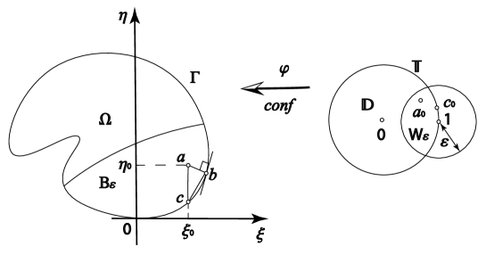
Figure 1. Construction from Lemma 2

For an arbitrary point $\zeta\in\gamma$ the quantity $|a-\zeta|^{2}=(\xi_{0}-\xi)^{2}+(\eta_{0}-\psi(\xi))^{2}$ attains its minimum at the point $\xi+i\psi(\xi)$ where $\xi$ is such that $(\xi_{0}-\xi)+\psi^{\prime}(\xi)(\eta_{0}-\psi(\xi))=0$. Notice that the latter equation is the equation of normal to $\gamma$ passed from the point $a$. Thus, the point $b\in\gamma$ nearest to $a$ belongs to the normal to $\gamma$ passing from $a$. Notice, that without loss of generality we may assume that $\xi>\xi_{0}$.

Denote by $\varDelta$ the triangle with vertexes at the points $a$, $b$ and $c$, and denote the angles at the vertices $a$, $b$ and $c$ of this triangle by $\beta(a)$, $\beta(b)$ and $\beta(c)$, respectively. Since the points $a$ and $b$ belong to the normal to $\varGamma$, then $b-a=k(\psi^{\prime}(\xi)-i)$ with $k\in\mathbb{R}$. Thus

$$\sin\beta(a)=\frac{|\psi^{\prime}(\xi)|}{\sqrt{1+\psi^{\prime}(\xi)^{2}}},\quad\text{and}\quad\cos\beta(c)=\frac{\psi^{\prime}(\widetilde{\xi})}{\sqrt{1+\psi^{\prime}(\widetilde{\xi})^{2}}},$$

where $\xi_{0}\leqslant\widetilde{\xi}\leqslant\xi$ (according to Lagrange’s mean value theorem). Since $\psi^{\prime}(0)=0$ and since $\xi-\xi_{0}$ is small when $\varepsilon$ is small enough, then both quantities $\sin\beta(a)$ and $\cos\beta(c)$ are also small and hence $\beta(a)\to 0$ and $\beta(c)\to\dfrac{\pi}{2}$ as $\varepsilon\to 0$. Therefore $\beta(b)\to\dfrac{\pi}{2}$ as $\varepsilon\to 0$. Applying the sine theorem to the triangle $\varDelta$ we obtain

$$\frac{|c-b|}{\sin\beta(a)}=\frac{|a-c|}{\sin\beta(b)},$$

which gives that

$$\frac{|c-b|}{|a-c|}=\frac{\sin\beta(a)}{\sin\beta(b)}\to 0$$

as $\varepsilon\to 0$. Hence, for sufficiently small $\varepsilon$ we have that $|c-b|<\varepsilon|a-c|$ for all $a\in B_{\varepsilon}$. Moreover, for all such $a$ we have

$$|(a-b)_{\tau}|\geqslant(1+\tau)\big{|}|a-c|-|b-c|\big{|}\geqslant(1+\tau)(1-\varepsilon)|a-c|.$$

It remains to use this estimate together with the following one

$$|a-c|=|\varphi(a_{0})-\varphi(c_{0})|\geqslant|a_{0}-c_{0}|\min_{z\in W_{\varepsilon}}|\varphi^{\prime}(z)|\geqslant(1-|a_{0}|)\min_{z\in W_{\varepsilon}}|\varphi^{\prime}(z)|,$$

where $c_{0}=\varphi^{-1}(c)$. The lemma is proved. ∎

Remark 4.

In the context of the problem under consideration we may assume that for any Jordan domain $B$ with smooth boundary the origin belongs to $\partial B$ and the tangent line to $B$ at this point is the real line. Indeed for any such domain $B$ the set $\partial B$ contains a point $w$ having minimum ordinate along $\partial B$. The tangent line to $\partial B$ at $w$ is horizontal. It remains to use shift moving $w$ to the origin, and recall that the operator $\mathcal{L}_{\tau}$ is invariant under such transformation of the plane (see Remark 2).

Combining Lemmas 1 and 2 together we have the next proposition that contains our central estimates.

Lemma 3.

Suppose all conditions of Lemmas 1 and 2 to be satisfied, and let $\varepsilon$ is taken from Lemma 2. Then for all $z\in W_{\varepsilon}=D(1,\varepsilon)\cap\mathbb{D}$ we have

(3.2) $$\big{|}\varphi^{\prime}(z)^{m}h^{(m)}(T\varphi(z))\big{|} \leqslant C\frac{m!R_{\varepsilon}^{m}}{(1+\tau)^{m}(1-\varepsilon)^{m}(1-|z|)^{m}}\|f\|_{\overline{G}},$$

(3.3) $$\big{|}\varphi^{\prime}(z)^{m}g^{(m)}(\varphi(z))\big{|} \leqslant C\frac{m!R_{\varepsilon}^{m}}{(1-|z|)^{m}}\|f\|_{\overline{G}},$$

where $R_{\varepsilon}=\dfrac{\max\{|\varphi^{\prime}(z)\colon z\in W_{\varepsilon}\}}{\min\{|\varphi^{\prime}(z)\colon z\in W_{\varepsilon}\}}$.

In fact we need to strengthen the estimates obtained in Lemma 3 in the case where the initial function $f\in C(\overline{G})\cap\mathcal{O}_{\tau}(G)$ is $\mathcal{L}_{\tau}$-analytic in some neighborhood of $\overline{G}$. Namely, the next proposition takes place.

Lemma 4.

Let $U$ be an open set such that $\overline{G}\subset U$ and let $f\in\mathcal{O}_{\tau}(U)$. Assume that all conditions of Lemmas 1 and 2 are fulfilled. Then for all $z\in W_{\varepsilon}=D(1,\varepsilon)\cap\mathbb{D}$ the estimate is satisfied

(3.4) $$\big{|}\overline{\varphi^{\prime}(z)}{}^{m}h^{(m)}(T\varphi(z))\big{|}\leqslant Cm!\bigg{(}\frac{1+\beta(\varepsilon)}{1+\tau}\bigg{)}^{m}\dfrac{\rho_{m}(z)}{(1-|z|)^{m}}\|f\|_{U},$$

where $\beta(\varepsilon)\to 0$ as $\varepsilon\to 0$, and

$$\rho_{m}(z)=\bigg{(}\frac{1-|z|}{R-|z|}\bigg{)}^{m}$$

for some number $R>1$.

To verify this lemma we need to apply Lemma 3 considering a conformal mapping from the disk $D(0,R)$ for some $R>1$ onto $G$ instead of $\varphi$ and taking into account the fact that $R_{\varepsilon}\big{/}(1-\varepsilon)$ in this case is $C_{1}(1+\beta(\varepsilon))$ with $\beta(\varepsilon)\to 0$ as $\varepsilon\to 0$ and with certain constant $C_{1}>0$.

The next simple statement may be readily verified using Green’s formula and integration by parts taking into account the facts that $1-|z|^{2}=0$ for $z\in\mathbb{T}$ and $\overline{\partial}(1-|z|^{2})=-z$, see [19], formula (2.3).

Lemma 5.

Let $F\in C^{\infty}(D(0,R))$ for some $R>1$. Then for any $k,N\in\mathbb{N}$, one has

(3.5) $$\int_{\mathbb{D}}(1-|z|^{2})^{k-1}\,F(z)\,z^{N-k+1}\,dm_{2}(z)=\frac{1}{k}\int_{\mathbb{D}}(1-|z|^{2})^{k}\,z^{N-k}\,\overline{\partial}F(z)\,dm_{2}(z).$$

Proof of Theorem 2.

According to Remark 4 one may (and shall) assume that $G$ and $\varphi$ satisfy all conditions of Lemma 2. Thus take $\varepsilon$ from this lemma and assume that $\zeta=1$.

Take a function $f\in C(\overline{G})\cap\mathcal{O}_{\tau}(G)$. According to (2.12) one has $f(z)=h(z_{\tau})+g(z)$, $z\in G$, where $g$ and $h$ are holomorphic functions in $G$ and $TG$, respectively. Let us assume for a moment that $f\in\mathcal{O}_{\tau}(U)$ for some open set $U$ that contains $\overline{G}$, so that the functions $g$ and $h$ are holomorphic in $U$ and $TU$, respectively. We will argue in the frameworks of this assumption. At the last step of the proof it remains to apply the regularization arguments based in the fact that the initial function $f$ can be approximated uniformly on $\overline{G}$ by functions $\mathcal{L}_{\tau}$-analytic in neighborhoods of $\overline{G}$ (each function in its own neighborhood).

In what follows we will use the following notations. For $k\in\mathbb{N}$ we put $\mu_{k}(z)=\overline{\varphi^{\prime}(z)}^{k}$, $z\in\overline{\mathbb{D}}$. We will write $A\lesssim B$ if $A\leqslant CB$ for some number $C>0$ which may depend on $\|\varPsi_{\varepsilon}\|$, $\|\overline{\partial}\varPsi_{\varepsilon}\|$, $\min_{z\in\overline{\mathbb{D}}}|\varphi^{\prime}(z)|$. Similarly, all constants in the usual “O-big” notation $\mathop{\mathbb{O}}(\cdot)$ may (and will) depend on these quantities. Moreover, for $k\in\mathbb{N}$ we put

$$F_{k}(z):=\frac{(-\tau)^{k}}{(k-1)!}\varPsi_{\varepsilon}(z)\,\mu_{k}(z)\,h^{(k)}(T\varphi(z)).$$

Direct computations based on the standard Green’s formula give that

(3.6) $$\mathcal{M}^{*}_{n,\varepsilon,\zeta}(f)=\int_{\mathbb{T}}\varPsi_{\varepsilon}(z)\,f(\varphi(z))\,z^{n}\,dz=2i\int_{\mathbb{D}}z^{n}\overline{\partial}[\varPsi_{\varepsilon}(z)f(\varphi(z))]\,dm_{2}(z)=\\ =2i\int_{\mathbb{D}}z^{n}f(\varphi(z))\,\overline{\partial}\varPsi_{\varepsilon}(z)\,dm_{2}(z)-2i\int_{\mathbb{D}}z^{n}F_{1}(z)\,dm_{2}(z).$$

It is clear that

$$\bigg{|}\int_{\mathbb{D}}z^{n}f(\varphi(z))\,\overline{\partial}\varPsi_{\varepsilon}(z)\,dm_{2}(z)\bigg{|}\leqslant\dfrac{2\pi\|\varPsi^{\prime}_{\varepsilon}\|\,\|f\|}{n+2},$$

and we need to estimate only the second summand in the right-hand side of (3.6). This estimate requires much more delicate considerations. The main idea how to estimate the quantity $\displaystyle\int_{\mathbb{D}}z^{n}F_{1}(z)\,dm_{2}(z)$, is to apply Lemma 5 to the functions $F_{k}$, $k\in\mathbb{N}$, consequently. Take an arbitrary $m\in\mathbb{N}$. Since

$$\overline{\partial}h^{(k)}(T\varphi(z))=-\tau\overline{\varphi^{\prime}(z)}h^{(k+1)}(T\varphi(z))$$

and $\mu_{k}(z)\overline{\varphi^{\prime}(z)}=\mu_{k+1}(z)$, we have

$$\int_{\mathbb{D}}F_{1}(z)z^{n}\,dm_{2}(z)= \int_{\mathbb{D}}(1-|z|^{2})z^{n-1}\,\overline{\partial}F_{1}(z)\,dm_{2}(z)$$

$$= -\tau\int_{\mathbb{D}}(1-|z|^{2})z^{n-1}\,\overline{\partial}[\varPsi_{\varepsilon}(z)\mu_{1}(z)]h^{\prime}(T\varphi(z))\,dm_{2}(z)$$

$$+\int_{\mathbb{D}}(1-|z|^{2})z^{n-1}\,F_{2}(z)\,dm_{2}(z)$$

$$= \cdots\;\cdots\;\cdots$$

$$= \sum_{k=1}^{m}\frac{(-\tau)^{k}}{k!}\int_{\mathbb{D}}(1-|z|^{2})^{k}z^{n-k}\overline{\partial}[\varPsi_{\varepsilon}(z)\mu_{k}(z)]h^{(k)}(T\varphi(z))\,dm_{2}(z)$$

$$+\int_{\mathbb{D}}(1-|z|^{2})^{m}z^{n-m}\,F_{m+1}(z)\,dm_{2}(z).$$

Let us estimate the integrals

$$I_{k}=\frac{(-\tau)^{k}}{k!}\int_{\mathbb{D}}(1-|z|^{2})^{k}z^{n-k}\overline{\partial}[\varPsi_{\varepsilon}(z)\mu_{k}(z)]h^{(k)}(T\varphi(z))\,dm_{2}(z),\quad k\in\mathbb{N}.$$

Observe that for $p\in\mathbb{N}$ and $\nu\in(0,1)$ it holds

(3.7) $$\int_{0}^{1}\dfrac{r^{p}\,dr}{(1-r)^{1-\nu}}\approx\dfrac{1}{\nu p^{\nu}}.$$

Let now $\beta(\varepsilon)$ be taken from Lemma 4, so that $\beta(\varepsilon)\to 0$ as $\varepsilon\to 0$. Then for sufficiently small $\varepsilon$ we have

(3.8) $$\frac{2\tau(1+\beta(\varepsilon))}{1+\tau}<\tau_{1}<1$$

for some $\tau_{1}\in(0,1)$ which may depend only on $\tau$ and $G$ (of course implicitly, via $\varphi$, $\varepsilon$, etc.). Since $(1-|z|^{2})^{k}\leqslant 2^{k}(1-|z|)^{k}$ for $z\in\mathbb{D}$, then using (3.4) and (3.8) we have

(3.9) $$|I_{k}|\leqslant C\tau^{k}\bigg{(}\frac{1+\beta(\varepsilon)}{1+\tau}\bigg{)}^{k}2^{k}\int_{D(z_{0},\varepsilon)}(1-|z|)^{k}\frac{k}{\varphi^{\prime}(z)}\frac{\rho_{k}(z)}{(1-|z|)^{k+1-\alpha}}|z|^{n-k}\,dm_{2}(z).$$

For $k<n$ this inequality together with (3.7) gives that

$$|I_{k}|=\mathop{\mathbb{O}}\Big{(}\frac{k\tau_{1}^{k}}{(n-k)^{\alpha}}\Big{)}.$$

For $k\geqslant n$ in order to estimate $I_{k}$ we will use next arguments. For $z\in W_{\varepsilon}=D(1,\varepsilon)\cap\mathbb{D}$ we have $r^{n-m}\leqslant(1-\varepsilon)^{n-k}$. Moreover, for sufficiently small $\varepsilon$ it holds that

$$\tau_{2}=\frac{\tau_{1}}{1-\varepsilon}<1.$$

So that for $k\geqslant n$ we have $|I_{k}|=\mathop{\mathbb{O}}(k\tau_{2}^{k})$.

It can be readily checked that

$$\sum_{k=1}^{n-1}\frac{k\tau_{1}^{k}}{(n-k)^{\alpha}}\lesssim\rho(n,\alpha,\tau),$$

where

$$\rho(n,\alpha,\tau_{1})=\frac{1}{n^{\alpha/2}}+\frac{n^{\alpha/4}\tau_{1}^{n^{\alpha/4}}}{1-\tau_{1}}+\frac{\tau_{1}^{n^{\alpha/4}+1}}{(1-\tau_{1})^{2}}.$$

Indeed it is enough to split the sum being estimate into two sums (where the first sum is taken over $k$ running from $0$ to the integer part of the number $n^{\alpha/4}$, while the second one is taken over remaining values of $k$) and to estimate directly both sums obtained. Moreover,

$$\sum_{k=n}^{\infty}k\tau_{2}^{k}=\frac{\tau_{2}^{n}}{1-\tau_{2}}\Big{(}n+\frac{\tau_{2}}{1-\tau_{2}}\Big{)}.$$

Since the last quantity tends to zero as $n\to\infty$, and since $\rho(n,\alpha,\tau_{1})\to 0$ as $n\to\infty$, then the integrals $\displaystyle\int_{\mathbb{D}}(1-|z|^{2})^{m}z^{n-m}\,F_{m+1}(z)\,dm_{2}(z)$ can be made arbitrary small by taking $m$ large enough. It gives, finally, that (3.1) takes place and the proof of Theorem 2 is completed. ∎

The remaining estimate (2.20) for $M_{n}=\mathcal{M}_{n,\varepsilon,\zeta}$ is the consequence of the following observation: for $P(z)=\sum_{k=-\nu}^{\nu}c_{k}z^{k}$ with integer $\nu>0$ and $c_{k}\in\mathbb{C}$, $-\nu\leqslant k\leqslant\nu$, we have

$$|\mathcal{M}_{n,\varepsilon,\zeta}(P)|=|\mathcal{M}_{n-\nu,\varepsilon,\zeta}(z^{\nu}P)|\leqslant A(n-\nu)^{-\alpha/2}\|P\|_{\mathbb{T}}$$

in view of (3.1), because for $Q=z^{\nu}P$ we have $Q\circ\varphi^{-1}\in C(\overline{G})\cap\mathcal{O}_{\tau}(G)$ since $Q\circ\varphi^{-1}$ is holomorphic in $G$.

Using the family of functionals $M_{n}=\mathcal{M}_{n,\varepsilon,\zeta}$ constructed in this section and follow the line of reasoning presented at the end of Section 2 we arrive to the complete proof of Theorem 1.

At the end of this section let us note that in the bianalytic case (that is for $\tau=0$) the estimate (3.1) can be improved a bit. Namely, for every function $f\in C(\overline{G})\cap\mathcal{O}(G,\overline{\partial}^{2})$ and for all sufficiently large integer $n$, it holds

$$\bigg{|}\int_{\mathbb{T}}f(\varphi(z))\,z^{n}\,dz\bigg{|}\leqslant A\frac{\|f\|_{\overline{G}}}{n^{\alpha}}.$$

The proof of this estimate may be obtained following the same scheme that was used in the proof of the estimate (3.1), but in this (in view of special algebraic structure of bianalytic functions) it is enough to use Green’s formula only twice and estimate thereafter the obtained integrals directly using (2.17) and applying Lemma 3 from [9] instead of Lemma 3.

4. Outline of the proof of the second statement in Theorem C

In this section we are going to present a schematic outline of the proof of the following proposition which is the second statement of Theorem C.

Proposition 1.

There exists a Jordan domain $G$ with Lipschitz boundary such that $G$ is $\overline{\partial}^{2}$-regular.

This result was obtained in [19], and its proof is very involved both substantively and technically. The construction of the desired domain $G$ is based on lacunary series technique, on variational principles of conformal mappings, and on Rudin–Carleson theorem about interpolation peak sets for continuous holomorphic functions.

The main aim of this section is to highlight the main steps of the construction of $\overline{\partial}^{2}$-regular domain $G$, and to show the way how the main difficulties of the corresponding construction may be overcome.

Let $G$ be a Jordan domain and $\varphi$ be some conformal mapping from $\mathbb{D}$ onto $G$, and assume that $\varphi$ is already extended to the eponymous homeomorphism from $\overline{\mathbb{D}}$ onto $\overline{G}$ according to the Carathéodory extension theorem. In order to satisfy the property that $G$ is $\overline{\partial}^{2}$-regular we need to have

(4.1) $$\int_{\mathbb{D}}|\varphi^{\prime\prime}(z)|\,dm_{2}(z)=\infty.$$

Indeed, otherwise the space of functions belonging to $C(\partial G)$ which are restrictions to $\partial G$ of some functions belonging to the space $C_{\overline{\partial}^{2}}(\overline{G})$ is a Baire first category set. This fact is proved in [19], Theorem 1; its proof may be obtained following the same scheme that was used above to prove Theorem 1 (see also the latter paragraph of Section 3), but the proof in the bianalytic case turns out to be rather simpler in view of some special properties bianalytic functions possessed in contrast to $\mathcal{L}_{\tau}$ analytic ones, $\tau\in(0,1)$.

Before constructing the univalent function $\varphi$ satisfying the above mentioned conditions, let us make one auxiliary construction. We need to construct the function $\psi\in C(\overline{\mathbb{D}})$ which is holomorphic in $\mathbb{D}$, such that $\psi^{\prime}\in H^{2}(\mathbb{D})$ (this condition is weaker than the univalence one) and for which the condition (4.1) is satisfied. Here $H^{p}(\mathbb{D})$, $p>0$, is the standard Hardy spaces in the unit disk. Let now $\psi$ be an arbitrary function that has the form

(4.2) $$\psi(z)=z+\sum_{k=k_{0}}\frac{z^{m_{k}}}{km_{k}},$$

where $m_{k}$, $k\geqslant k_{0}$, are positive integers such that the lacunary conditions are fulfilled

$$\frac{m_{k+1}}{m_{k}}>2,\qquad\sum_{n=2}^{\infty}\sum_{k=1}^{n-1}\frac{m_{k}}{m_{n}}<\infty.$$

It is clear that $\psi\in C(\overline{\mathbb{D}})$ and the condition (4.1) is an immediate consequence of the fact that the series $\sum_{k=1}^{\infty}k^{-1}$ diverges. Unfortunately, for functions of the form (4.2) the condition (4.1) forbids completely the univalence of $\psi$. But the following important results takes place (see [19], Lemma 3.2 and Theorem 3).

Proposition 2.

For every function $f\in C(\mathbb{T})$ and for every function $\psi$ of the form (4.2) there exists a couple $(\varPhi_{1},\varPhi_{2})$ of functions holomorphic in $\mathbb{D}$ such that the function $F_{f}=\varPhi_{1}\overline{\psi}-\varPhi_{2}$ is extended continuously to $\mathbb{T}$ and satisfies the conditions $\sup_{z\in\mathbb{D}}|F_{f}(z)|\leqslant 2\|f\|_{\mathbb{T}}$ and $F_{f}=f$ on $\mathbb{T}$.

In connection to this proposition one ought to note that the functions $\varPhi_{1}$ and $\varPhi_{2}$ separately do not belong to any of the spaces $H^{p}(\mathbb{D})$ as $p>0$, and only the function $F_{f}$ possesses the good properties mentioned above.

In spite of the circumstance that the function $\psi$ from (4.2) is never univalent in $\mathbb{D}$ (see, for instance, [28], Section 5.4), Proposition 2 is an important ingredient of the construction of domain $G$ from Proposition 1. The desired domain $G$ may be constructed as an image a certain Lipschits domain $\Omega\subset\mathbb{D}$ under conformal mapping by univalent and Lipschitz in $\Omega$ function $\varphi$, where $\Omega$ is obtained as a small perturbation of $\mathbb{D}$, while $\varphi$ is obtained as a small perturbation of $\psi$ with respect to the $L^{2}$-norm on the boundary.

The desired domain $\Omega$ is constructed as a kernel of a decreasing sequence of Jordan domains $\Omega_{j}$, $j=0,1,2\ldots$, where $\Omega_{0}=\mathbb{D}$, with uniform estimate of Lipschitz constants of their boundaries. Let us describe the first step of this construction. The domain $\Omega_{1}$ is obtained from $\Omega_{0}=\mathbb{D}$ using the celebrated Privalov’s ice-cream cone construction, see [17], Chapter III, Section D. Indeed, the $L^{2}$-norm of the function $\psi^{\prime}-1$ on $\mathbb{T}$ can be made arbitrary small together with the quantity $\sum_{k=k_{0}}^{\infty}k^{-2}$; the same takes place for $L^{2}$-norm of the corresponding non-tangential maximal function. Thus, for a given $\delta>0$ and for sufficiently large $k_{0}=k_{0}(\delta)$ there exists a domain $\Omega_{1}=\Omega_{0}\setminus\bigcup_{\alpha\in A}T_{\alpha}$, where $A$ is at most countable set of indices and $T_{\alpha}$, $\alpha\in A$, are mutually disjoint closed isosceles triangles with the bases on $\partial\Omega_{0}$ such that the function $\psi^{\prime}$ is continuous on $\overline{\Omega}_{1}$ and such that everywhere on $\overline{\Omega}_{1}$ it holds $|\psi^{\prime}(z)-1|<\delta$. Moreover, the triangles $T_{\alpha}$, $\alpha\in A$ may be chosen such that the angles at the base of every $T_{\alpha}$ are less than $\delta$, and the sum of perimeters of all $T_{\alpha}$, $\alpha\in A$ is also less than $\delta$.

The part of the boundary $\partial\Omega_{1}$ that does not belong to $\partial\Omega_{0}$ consists of at most countable family of intervals of the total length $\ell<\delta$. Our aim is to modify the function $\psi$ on these intervals. Take a finite family of pairwise disjoint closed segments of the total length greater than $0.9\,\ell$ belonging to the intervals of this family. For every such segment $I$ let us proceed as follows.

Let $Q$ be a circular lune whose boundary consists of $I$ and the circular arc $I^{\prime}$ of some circle with center lying outside $\Omega_{1}$ and with the angle measure less than $\delta^{2}$ (the arcs $I$ and $I^{\prime}$ intersect only by their end-points). Take a function $\chi$ that maps conformally the exterior of $Q$ onto $\mathbb{D}$ with the normalization $\chi(\infty)=0$ and assume that $\chi$ is already extended to the homeomorphism of the corresponding closed domains. Define

$$\psi_{I}(z)=\sum_{k=k_{0}(I)}^{\infty}\frac{(\chi(z))^{m_{k}}}{km_{k}},$$

where $k_{0}(I)$ is sufficiently large. At the next step we remove from $\Omega_{1}$ all domains $Q$ constructed above and all isosceles triangles constructed on all arcs $I^{\prime}$ using the ice-cream cone construction as it was mentioned above. The resulting domain will be $\Omega_{2}$. For this domain we repeat the same construction as before.

It can be readily verified that the result of Proposition 2 will be preserved if replace the function $\psi$ with $\psi(z)-z$. Therefore we can use the function $\psi_{I}$ constructed above for modification of the initial function $\psi$. Indeed, we can define $\varphi=\psi+\sum_{I}\psi_{I}$, where the sum is taken over all $\psi_{I}$ constructed in all steps. It is not difficult to prove that $\varphi$ is univalent in the resulting domain $\Omega$ which is the kernel of the sequence $\Omega_{j}$, $j\geqslant 0$.

Finally, we need to check that the domain $\Omega$ is $\overline{\partial}^{2}$-regular. In order to verify this property we will use the following criterion of $\overline{\partial}^{2}$-regularity, which was proved in [19], Lemma 4.2, and which is obtained using the functional analysis methods and the Rudin–Carleson theorem stating that any compact set of zero length is an interpolation peak set for continuous holomorphic functions, see [30] and [8].

Proposition 3.

The domain $G$ is $\overline{\partial}^{2}$-regular if and only if the following property is satisfied. There exists an increasing sequence $(E_{n})$, $n=1,2,\ldots$, of closed subsets of $\partial G$ such that

1) the length of the set $\partial G\setminus\bigcup_{n}E_{n}$ is zero, and

2) for every $f\in C(\partial G)$ with $\|f\|_{\partial G}\leqslant 1$, for every $E_{n}$, and for every $\varepsilon>0$ there exists $F\in C(\overline{G})\cap\mathcal{O}(G,\overline{\partial}^{2})$ such that $|F(z)|\leqslant 2$ for $z\in G$ and $|f(z)-F(z)|<\varepsilon$ for $z\in E_{n}$.

5. Uniform approximation by $\mathcal{L}$-analytic
polynomials and $\mathcal{L}$-Dirichlet problem

Denote by $\mathcal{P}$ the class of all polynomials in the complex variable $z$. Let $\mathcal{L}\in\operatorname{\mathcal{E}}$, and let $\lambda_{1}$ and $\lambda_{2}$ be the characteristic roots of $\mathcal{L}$. Recall that by $\mathcal{L}$-analytic polynomial we mean any complex-valued polynomial $P$ in two real variables that satisfies the equation $\mathcal{L}P=0$. If $\lambda_{1}\neq\lambda_{2}$, then any $\mathcal{L}$-analytic polynomial has the form (2.2), where $f_{1},f_{2}\in\mathcal{P}$. If $\lambda_{1}=\lambda_{2}$, then any $\mathcal{L}$-analytic polynomial is the function of the form (2.3), where also $f_{0},f_{1}\in\mathcal{P}$. Denote by $\mathcal{P}_{\mathcal{L}}$ the class of all $\mathcal{L}$-analytic polynomials.

Note that if we reduce the operator $\mathcal{L}$ to the form (2.6) with $\tau\in[0,1)$ or (2.7) with $\tau\in(0,1)$, respectively, then $\mathcal{L}$-analytic polynomials will take the form (2.11) or (2.12), respectively, where $g,h\in\mathcal{P}$. Moreover, any $\mathcal{L}_{0}$-analytic polynomials has the form $\overline{z}P_{1}(z)+P_{0}(z)$ with $P_{0},P_{1}\in\mathcal{P}$ (since $\mathcal{L}_{0}=\overline{\partial}{}^{2}$).

For a given compact set $X\subset\mathbb{C}$ we denote by $P_{\mathcal{L}}(X)$ the space of all functions that can be approximated uniformly on $X$ by $\mathcal{L}$-analytic polynomials. In other words, a function $f$ belongs to $P_{\mathcal{L}}(X)$ if and only if for every $\varepsilon>0$ there exists $P\in\mathcal{P}_{\mathcal{L}}$ such that $\|f-P\|_{X}<\varepsilon$. It is clear that

$$P_{\mathcal{L}}(X)\subset C_{\mathcal{L}}(X):=C(X)\cap\mathcal{O}(X^{\circ},\mathcal{L}),$$

where $X^{\circ}=\operatorname{Int}(X)$ is the interior of $X$. Let us consider the following problem.

Problem 2.

To describe compact sets $X\subset\mathbb{C}$ for which $P_{\mathcal{L}}(X)=C_{\mathcal{L}}(X)$.

More precisely, it is demanded in Problem 2 to obtain necessary and sufficient conditions on $X$ in order that the equality $P_{\mathcal{L}}(X)=C_{\mathcal{L}}(X)$ is satisfied. This problem is the well-known classical problem in complex analysis. Its statement is traced to the classical problems on uniform approximation by harmonic polynomials and by polynomials in the complex variables that were solved by Walsh and Mergelyan, respectively. One ought to emphasize that Problem 2 is still open in the general case. We refer the interested reader to [22], where one can find a detailed survey concerning the matter. Let us also note that Problem 2 is closely related with the problem on approximation of functions $f\in C_{\mathcal{L}}(X)$ by functions which are $\mathcal{L}$-analytic in neighborhoods of $X$. This is a classical problem in the case of holomorphic and harmonic functions and its consideration is out of the scope of this paper. The studies of this problem in the context of approximation by solutions of general elliptic equations was started in 1980s–1990s. A more or less exhaustive bibliography on this subject may be found in [22], but let us mention here a couple of important works [26], [31], [34], [35] and [36].

The only case where Problem 2 was solved completely is the case $\mathcal{L}=\Delta$, and, as a clear consequence, a slightly more general case when $\mathcal{L}$ has real coefficients (up to a common complex multiplier). To state the corresponding result we need the concept of a Carathéodory compact set.

We recall, that a compact set $X\subset\mathbb{C}$ is called a Carathéodory compact set, if $\partial X=\partial\widehat{X}$, where $\widehat{X}$ denotes the union of $X$ and all bounded connected components of $\mathbb{C}\setminus X$.

Theorem E.

Let $X$ be a compact set in $\mathbb{C}$. Then $P_{\Delta}(X)=C_{\Delta}(X)$ if and only if $X$ is a Carathéodory compact set.

This remarkable result was proved by Walsh at the end of 1920s, see [38], and nowadays it is called the Walsh–Lebesgue theorem in view of the crucial role the Lebesgue theorem (Theorem A) plays in the proof. Note that in [38] only the case of nowhere dense compact sets was considered explicitly, but the general case may be obtained as a consequence of this partial result. Let us also observe that the first, to the best of our knowledge, formulation of the Walsh–Lebesgue theorem in the above form was presented in [24], Section 1. The deep enough exposition of the Walsh–Lebesgue theorem and certain related topics may be found in Chapter 2 of the book [15].

The second case, when the substantial progress was achieved in studies of Problem 2, is the case where $\mathcal{L}=\overline{\partial}{}^{2}$. In this case Problem 2 was solved completely for Carathéodory compact sets. The following results was obtained in [11], Theorem 2.2.

Theorem F.

Let $X$ be a Carathéodory compact set in $\mathbb{C}$. Then $P_{\overline{\partial}^{2}}(X)=C_{\overline{\partial}^{2}}(X)$ if and only if any bounded connected component of the set $\mathbb{C}\setminus X$ is not a Nevanlinna domain.

The concept of a Nevanlinna domain is the special analytic characteristic of bounded simply connected domains in $\mathbb{C}$. It’s formal definition is given in [13], Definition 1, in the case of Jordan domains with rectifiable boundaries, and in [11], Definition 2.1, in the general case. We are not going to define this concept explicitly here, but we ought to note that the property of a given domain $G$ in $\mathbb{C}$ to be a Nevanlinna domain consists in the possibility of representing the function $\overline{z}$ almost everywhere on $\partial G$ in the sense of conformal mappings as a ratio of two bounded holomorphic functions in $G$. The properties of Nevanlinna domains has been studied in detail during the two last decades (see, for instance, [14, 3, 20, 4, 21, 6, 5]. It was shown that the class of Nevanlinna domains is rather big in spite of the fact that the definition of a Nevanlinna domain imposes quite rigid condition to the boundary of the domain under consideration. For instance, there exists such Nevanlinna domains $G$ that the Hausdorff dimension of $\partial G$ could take any value in $[1,2]$ (see [5], Theorem 3).

For compact sets $X$ which are not Carathéodory compact sets the question whether the equality $P_{\overline{\partial}^{2}}(X)=C_{\overline{\partial}^{2}}(X)$ holds or not, is solved only for some particular cases. In the general case the answer to this question is know only in the form of a certain approximability condition of a reductive nature. For certain non-Carathéodory compact sets of a special form the sufficient approximability conditions were obtained in [7], [11] and [10]. One interesting and helpful tool using in these works is the concept of an analytic balayage of measures which was introduced by D. Khavinson [16], which was rediscovered in [11] in a slightly different terms, and which was studied by several authors both as an object of an independent interest and in connection with properties of badly approximable functions in $L^{p}(\mathbb{T})$ (see [1] and bibliography therein). It seems to us interesting and appropriate to note this point.

In order to proceed further with our discussions of Problem 2 and its relations with $\mathcal{L}$-Dirichlet problem let us introduce one more space of functions. For a pair of compact sets $X$ and $Y$ in $\mathbb{C}$ with $X\subseteq Y$, let $A_{\mathcal{L}}(X,Y)$ be the closure in $C(X)$ of the space $\{f|_{X}\colon f\in\mathcal{O}(U_{f}(Y),\mathcal{L})\}$, where $U_{f}(X)$ is some, depending on $f$, neighborhood of $Y$. The typical case when we are needed this space, is the case when $X=\partial G$ and $Y=\overline{G}$ for some bounded simply connected domain $G$ in $\mathbb{C}$. It is clear, that

$$P_{\mathcal{L}}(X)\subset A_{\mathcal{L}}(X,Y)\subset A_{\mathcal{L}}(X,X)\subset C_{\mathcal{L}}(X).$$

Let us also note that if $X$ has a connected complement, then $A_{\mathcal{L}}(X,Y)=P_{\mathcal{L}}(X)$ for every $Y$ with $X\subseteq Y$. This is a direct consequence of the standard Runge’s pole shifting method which remains valid for $\mathcal{L}$-analytic functions, see [23], Section 3.10.

Although a complete solution to Problem 2 has not yet been obtained (for any operator $\mathcal{L}$ under consideration, except for the Laplace operator $\Delta$ and for operators that can be reduced to it by a not degenerate real-linear transformation of the plane), the following approximability criterion of a reductive nature was established in connection with this problem in the early 2000s.

Theorem G.

Let $X$ be a compact set in $\mathbb{C}$ having disconnected complement, and let $\mathcal{L}$ be an arbitrary operator of the form (1.1). The equality $P_{\mathcal{L}}(X)=C_{\mathcal{L}}(X)$ takes place if and only if for every connected component $G$ of the set $\operatorname{Int}(\widehat{X})$ such that $G\cap(\mathbb{C}\setminus X)\neq\emptyset$ the equality is satisfied

$$A_{\mathcal{L}}(\overline{G}\cap X,\overline{G})=C_{\mathcal{L}}(\overline{G}\cap X).$$

This theorem was firstly proved in [7] for bianalytic functions, and almost immediately after that the proof was modified for general $\mathcal{L}$ in [40]. Theorem G allows us to reduce the problem of $\mathcal{L}$-analytic polynomial approximation on a given compact set $X$ to compact subsets of $X$ having more simple topological structure.

In the particular case, when $X$ is a Carathéodory compact set, Theorem G gives that the equality $P_{\mathcal{L}}(X)=C_{\mathcal{L}}(X)$ takes place if and only if for any bounded connected component $G$ of the set $\mathbb{C}\setminus X$ one has $A_{\mathcal{L}}(\partial G,\overline{G})=C(\partial G)$. In this case the domain $G$ under consideration is such that $\partial G=\partial G_{\infty}$, where $G_{\infty}$ is the unbounded connected component of the set $\mathbb{C}\setminus\overline{G}$. Such domain $G$ is called a Carathéodory domain. It is clear that every Carathéoodry domain is simply connected and possesses the property $G=\operatorname{Int}(\overline{G})$.

Given a bounded simply connected domain $\Omega$ let us denote by $\partial_{a}\Omega$ the accessible part of $\partial\Omega$, namely the set of all points $\zeta\in\partial\Omega$ which are accessible from $G$ by some Jordan curve lying in $G\cup\{\zeta\}$ and ending at $\zeta$.

We are going to present one criterion in order that the equality $A_{\mathcal{L}}(\partial G,\overline{G})=C(\partial G)$ holds for a given Carathéodory domain $G$ (see Theorem 3 below). This result was firstly obtained in [39], but the proof given therein is not enough complete in a certain place. To state Theorem 3 we need to introduce yet another space of functions and give one more definition. Let $G$ be a Carathéodory domain in $\mathbb{C}$, and let $\varphi$ be some conformal mapping from $\mathbb{D}$ onto $G$. One says that a holomorphic function $f$ in $G$ belongs to the space $\operatorname{\mathit{AC}}(G)$, if the function $f\circ\varphi$ is extendable to a function which is continuous on $\overline{\mathbb{D}}$ and absolutely continuous on $\mathbb{T}$. It follows from the standard facts about conformal mappings, that for every function $f\in\operatorname{\mathit{AC}}(G)$, for every point $\zeta\in\partial_{a}G$, and for every path $\varUpsilon$ lying in $G\cup\{\zeta\}$ and ending at $\zeta$, the limit of $f$ along $\varUpsilon$ exists and is equal to the same value $f(\zeta)$, which is called a boundary value of $f$ at $\zeta$.

Definition 3.

Let $\mathcal{L}$ be an operator of the form (1.1) with characteristic roots $\lambda_{1}\neq\lambda_{2}$. A Carathéodory domain $G$ is called an $\mathcal{L}$-special domain, if there exist two functions $F_{1}\in\operatorname{\mathit{AC}}(T_{(1)}G)$ and $F_{2}\in\operatorname{\mathit{AC}}(T_{(2)}G)$ such that for every $\zeta\in\partial_{a}G$ one has $F_{1}(T_{(1)}\zeta)=F_{2}(T_{(2)}\zeta)$.

The real linear transformations $T_{(1)}$ and $T_{(2)}$ of the plane are defined just after the formula (2.2) in Section 2 above.

Theorem 3.

Let $G$ be a Carathéodory domain in $\mathbb{C}$ and let $\mathcal{L}$ be an operator of the form (1.1) with characteristic roots $\lambda_{1}\neq\lambda_{2}$.

1) The equality $A_{\mathcal{L}}(\partial G,\overline{G})=C(\partial G)$ takes place if and only if the domain $G$ is not an $\mathcal{L}$-special domain.

2) If $\mathcal{L}\in\operatorname{\mathcal{S}\mathcal{E}}$ then every Carathéodory domain in $\mathbb{C}$ is not $\mathcal{L}$-special.

Proof.

Let $\varphi$ be a conformal mapping from $\mathbb{D}$ onto $G$ and let $\psi$ be the respective inverse mapping. Without lost of generality we may assume that $\varphi$ has angular boundary value at the point $1$. By virtue of [29], Propositions 2.14 and 2.17, we have $\partial_{a}G=\{\varphi(\xi)\colon\xi\in\mathcal{F}(\varphi)\}$, where $\mathcal{F}(\varphi)$ is the Fatou set of $\varphi$, that is the set of all points $\xi\in\mathbb{T}$, where $\varphi$ has finite angular boundary values $\varphi(\xi)$ according to the classical Fatou’s theorem. As it was shown in [10], $\partial_{a}G$ is a Borel set. In view of [10], Corollary 1, the functions $\varphi$ and $\psi$ can be extended to Borel measurable functions (denoted also by $\varphi$ and $\psi$) on $\mathbb{D}\cup\mathcal{F}(\varphi)$ and $G\cup\partial_{a}G$ respectively in such a way, that $\varphi(\psi(\zeta))=\zeta$ for all $\zeta\in\partial_{a}G$ and $\psi(\varphi(\xi))=\xi$ for all $\xi\in\mathcal{F}(\varphi)$.

Let $\omega$ be the measure on $\partial G$ defined by $\omega:=\varphi(d\xi)$ (see [10], Section 3, for detailed construction of this measure and its properties). In fact $\omega$ is a measure on $\partial_{a}G$ and has no atoms. Moreover, $|\omega(\cdot)|=2\pi\omega(\varphi(0),\cdot,G)$, where $\omega(\varphi(0),\cdot,G)$ is the harmonic measure on $\partial G$ evaluated with respect to $\varphi(0)$ and $G$.

Taking into account Remark 1 we assume that $\mathcal{L}$ is already reduced to the form $c\mathcal{L}^{\dagger}_{\tau}$, $\tau\in[0,1)$ in the case where $\mathcal{L}$ is strongly elliptic, or to the form $c\mathcal{L}_{\tau}$, $\tau\in(0,1)$, in the opposite case. Since the further constructions are actually the same in both these cases, we will deal in details only with the case $\mathcal{L}=\mathcal{L}_{\tau}$. Let us recall that $z_{\tau}=z-\tau\overline{z}$ and $T\colon z\mapsto z_{\tau}$.

Suppose that $G$ is such that $A_{\tau}(\partial G,\overline{G}):=A_{\mathcal{L}_{\tau}}(\partial G,\overline{G})\neq C(\partial G)$. It means that there exists a (finite complex-valued Borel) measure $\mu$ on $\partial G$ which is orthogonal to the space $A_{\tau}(\partial G,\overline{G})$. In view of (2.12) the orthogonality of $\mu$ to $A_{\tau}(\partial G,\overline{G})$ means that $\mu$ is orthogonal to the space $R(\overline{G})$ consisting of functions which can be approximated uniformly on $\overline{G}$ by rational functions in the complex variable with poles lying outside $\overline{G}$ and to the space $\{h(z_{\tau})\colon h\in R(T\overline{G})\}$. The orthogonality of $\mu$ to $R(\overline{G})$ means that $\int f\,d\mu=0$ for every $f\in R(\overline{G})$.

Since $\mu$ is orthogonal to $R(\overline{G})$, then, according to [10], Theorem 2, there exists a function $b$ belonging to the Hardy space $H^{1}(\mathbb{D})$ in the unit disk such that

$$\mu=(b\circ\psi)\,\omega.$$

Let $\varPhi$ be some primitive to $b$ in $\mathbb{D}$. According to [27], Section II.5.7, $\varPhi\in C(\overline{\mathbb{D}})$ and $\varPhi$ is absolutely continuous on $\mathbb{T}$. Moreover, for any point $\xi\in\mathbb{T}$ we have $\varPhi(\xi)=\varPhi(1)+\nu(\varUpsilon_{\xi})$, where $\nu$ is the measure on $\mathbb{T}$ defined by the setting $d\nu=b\,d\xi$, and $\varUpsilon_{\xi}$ is the arc of $\mathbb{T}$ running from $1$ to $\xi$ in the positive direction. Finally, let $F(z)=\varPhi(\psi(z))$, $z\in G$. Since $G$ is a Carathéodory domain, for any point $\zeta\in\partial_{a}G$ there exists a unique point $\xi\in\mathbb{T}$ such that $\xi\in\mathcal{F}(\varphi)$ and $\varphi(\xi)=\zeta$, see [10], Proposition 1. Therefore, $F$ is well-defined on $\partial_{a}G$ and $F\in\operatorname{\mathit{AC}}(G)$.

Next we do the same thing for the domain $G_{\tau}:=TG$, which is a Carathéodory one, and for which it holds $\partial_{a}G_{\tau}=T(\partial_{a}G)$. Let $\varphi_{\tau}$ be some conformal mapping from $\mathbb{D}$ onto $G_{\tau}$ such that $1\in\mathcal{F}(\varphi_{\tau})$ and $T\varphi(1)=\varphi_{\tau}(1)$. As previously we denote by $\psi_{\tau}$ the inverse mapping for $\varphi_{\tau}$ in $G_{\tau}$ and by $\omega_{\tau}$ the measure $\varphi_{\tau}(d\xi)$ on $\partial G_{\tau}$. Furthermore, let $\mu_{\tau}$ be the measure on $\partial G_{\tau}$ defined by the setting $\mu_{\tau}(E)=\mu(T^{-1}E)$, where $E$ is a Borel set. It is clear that $\mu_{\tau}$ is orthogonal to $R(\overline{G_{\tau}})$.

Repeating the construction of $b$, $\varPhi$, $\nu$ and $F$ given above, using $\mu_{\tau}$, $\varphi_{\tau}$ and $\psi_{\tau}$ instead of $\mu$, $\varphi$, and $\psi$, respectively, we obtain the function $b_{\tau}\in H^{1}(\mathbb{D})$ such that $\mu_{\tau}=(b_{\tau}\circ\psi_{\tau})\,\omega_{\tau}$, and take $\varPhi_{\tau}$ to be the primitive of $b_{\tau}$ such that $\varPhi_{\tau}(1)=\varPhi(1)$. We have used here the fact that $\varPhi_{\tau}\in C(\overline{\mathbb{D}})$. Finally we put $F_{\tau}(w)=\varPhi_{\tau}(\psi_{\tau}(w))$, $w\in G_{\tau}$, so that $F_{\tau}\in\operatorname{\mathit{AC}}(G_{\tau})$.

It remains to show, how the functions $F$ and $F_{\tau}$ are related to each other. Let $\varGamma$ is a closed Jordan curve and let $\varOmega$ be the domain bounded by $\varGamma$. Take three points $\zeta_{1},\zeta_{2},\zeta_{3}\in\varGamma$. One says that a triplet $(\zeta_{1},\zeta_{2},\zeta_{3})$ is positive with respect to $\varOmega$, if $\zeta_{2}$ lies on the arc of $\varGamma$ running from $\zeta_{1}$ to $\zeta_{3}$ in the positive direction on $\varGamma$ (with respect to $\varOmega$).

Let $\alpha,\xi\in\mathbb{T}\cap\mathcal{F}(\varphi)$ are such that the triplet $(1,\alpha,\xi)$ is positive with respect to $\mathbb{D}$. Let $\alpha^{\prime}=\psi_{\tau}(T\varphi(\alpha))$ and $\xi^{\prime}=\psi_{\tau}(T\varphi(\xi))$.

We claim that the triplet $(1,\alpha^{\prime},\xi^{\prime})$ is also positive with respect to $\mathbb{D}$. Assuming this claim already proved, let us finish the proof of Theorem 3. Since the triplets $(1,\alpha,\xi)$ and $(1,\alpha^{\prime},\xi^{\prime})$ are both positive with respect to $\mathbb{D}$, and since the sets $\mathcal{F}(\varphi)$ and $\mathcal{F}(\varphi_{\tau})$ are everywhere dense in $\mathbb{T}$, then for the arc $\varUpsilon_{\xi}$ defined above we have

(5.1) $$\psi_{\tau}(T\varphi(\varUpsilon_{\xi}\cap\mathcal{F}(\varphi)))=\varUpsilon_{\xi^{\prime}}\cap\mathcal{F}(\varphi_{\tau}).$$

Using this equality we have that for $\zeta=\varphi(\xi)\in\partial_{a}G$ and $\xi^{\prime}=\psi_{\tau}(T\zeta)$ it holds

$$F_{\tau}(T\zeta)-\varPhi_{\tau}(1) =\varPhi_{\tau}(\xi^{\prime})-\varPhi_{\tau}(1)=\nu_{\tau}(\varUpsilon_{\xi^{\prime}}\cap\mathcal{F}(\varphi_{\tau}))$$

$$=\mu_{\tau}(\varphi_{\tau}(\varUpsilon_{\xi^{\prime}}\cap\mathcal{F}(\varphi_{\tau})))=\mu_{\tau}(T\varphi(\varUpsilon_{\xi}\cap\mathcal{F}(\varphi)))$$

$$=\mu(\varphi(\varUpsilon_{\xi}\cap\mathcal{F}(\varphi)))=\nu(\varUpsilon_{\xi}\cap\mathcal{F}(\varphi))=\varPhi(\xi)-\varPhi(1)$$

$$=F(\zeta)-\varPhi(1).$$

Since $\varPhi_{\tau}(1)=\varPhi(1)$ we finally have that $F_{\tau}(T\zeta)=F(\zeta)$ for every $\zeta\in\partial_{a}G$, as demanded in Definition 3 and Theorem 3.

It remains to prove our claim stating that the triplet $(1,\alpha^{\prime},\xi^{\prime})$ is positive whenever the initial triplet $(1,\alpha,\xi)$ is positive (with respect to $\mathbb{D}$).

For two points $p,q\in\mathbb{T}$ let $C_{p,q}$ be some circular arc belonging to $\mathbb{D}\cup\{p,q\}$ that starts at $p$, ends at $q$ and intersects $\mathbb{T}$ at both $p$ and $q$ non-tangentially. Let $\Omega_{1,\alpha,\xi}$ be the Jordan domain bounded by the closed Jordan curve $\varGamma_{1,\alpha,\xi}=C_{1,\alpha}\cup C_{\alpha,\xi}\cup C_{\xi,1}$, where we assume that $C_{1,\alpha}$, $C_{\alpha,\xi}$ and $C_{\xi,1}$ are taken in such a way that $\varGamma_{1,\alpha,\xi}$ is a closed Jordan curve, and $0\in\Omega_{1,\alpha,\xi}$. It is clear that the triplet $(1,\alpha,\xi)$ is positive with respect to $\Omega_{1,\alpha,\xi}$.

Since $\alpha$ and $\xi$ are Fatou points for $\varphi$, and since all three arcs $C_{1,\alpha}$, $C_{\alpha,\xi}$ and $C_{\xi,1}$ intersects $\mathbb{T}$ non-tangentially, we have $\varphi\in C(\overline{\Omega}_{1,\alpha,\xi})$. Moreover, since $G$ is a Carathéodory domain, then for each point $\zeta\in\partial_{a}G$ there exists a unique point $\eta\in\mathcal{F}(\varphi)$ such that $\varphi(\eta)=\zeta$ (see [10], Proposition 1), and hence $\varphi$ is injective on $\overline{\Omega}_{1,\alpha,\xi}$. Finally, in view of the Carathéodory extension theorem (see, for instance, [29], Theorem 2.6) the domain $\varphi(\Omega_{1,\alpha,\xi})\subset G$ is a Jordan domain. Furthermore, the triplet $(\varphi(1),\varphi(\alpha),\varphi(\xi))$ is positive with respect to $\varphi(\Omega_{1,\alpha,\xi})$ (it can be readily verified by direct computation of index of the curve $\varphi(\varGamma_{1,\alpha,\xi}$ with respect to the point $\varphi(0)\in\varphi(\Omega_{1,\alpha,\xi})$). Since $T$ is sense-preserving mapping, then the triplet $(\varphi_{\tau}(1),\varphi(\alpha^{\prime}),\varphi(\xi^{\prime}))=(T\varphi(1),T\varphi(\alpha),T\varphi(\xi))$ is positive with respect to the domain $T\varphi(\Omega_{1,\alpha,\xi})$.

Let us consider the domain $\Omega^{\prime}=\psi_{\tau}(T\varphi(\Omega_{1,\alpha,\xi}))\subset\mathbb{D}$. It is clear that $\partial\Omega^{\prime}\subset\mathbb{D}\cup\{1,\alpha^{\prime},\xi^{\prime}\}$. Repeating the arguments used above we conclude that $\Omega^{\prime}$ is a Jordan domain and $\varphi_{\tau}$ is continuous and injective on $\overline{\Omega^{\prime}}$. Therefore the triplet $(1,\alpha^{\prime},\xi^{\prime})$ is positive with respect to $\mathbb{D}$, as it was claimed.

Let us briefly explain how to proceed in the remaining case, namely in the case when $\mathcal{L}$ is reduced to the form $c\mathcal{L}^{\dagger}_{\tau}$. For a given set $E\subset\mathbb{C}$ we put $E_{C}=\{\overline{z}\colon z\in E\}$. Similarly to the previous case we consider some measure $\mu$ on $\partial G$ orthogonal to $A_{\mathcal{L}^{\dagger}_{\tau}}(\partial G,\overline{G})$. In view of (2.11) it means that $\mu$ is orthogonal to the space $\{g(\overline{z})\colon g\in R(\overline{G_{C}})\}$ and to the space $\{h(z_{\tau})\colon h\in R(\overline{G_{\tau}})\}$. The first orthogonality condition yields that the measure $\mu_{C}$ defined by the setting $\mu_{C}(E)=\mu(E_{C})$ on $\partial G_{C}$ is orthogonal to $R(\overline{G_{C}})$.

Now we can repeat the constructions of $F$ and $F_{\tau}$ given above using $\mu_{C}$ instead of $\mu$ and keeping $\mu_{\tau}$ unchanged. Doing this we obtain the functions $F\in\operatorname{\mathit{AC}}(G_{C})$ and $F_{\tau}\in\operatorname{\mathit{AC}}(G_{\tau})$ such that $-F(\overline{z})=F_{\tau}(z_{\tau})$ for all $z\in\partial_{a}G$. The negative sign at the left-hand side of this equality is related with the following circumstance. Let $(1,\alpha,\xi)$ be a positive (with respect to $\mathbb{D}$) triplet of points in $\mathbb{T}\cap\mathcal{F}(\varphi)$, let $\varphi_{C}$ be some conformal mapping from $\mathbb{D}$ onto $G_{C}$ such that $1\in\mathcal{F}(\widetilde{\varphi})$ and $C\varphi(1)=\widetilde{\varphi}(1)$, and let $\psi_{C}=\varphi_{C}^{-1}$. Then the triplet $(1,\alpha^{\prime\prime},\xi^{\prime\prime})$, where $\alpha^{\prime\prime}=\psi_{C}(\overline{\varphi(\alpha)})$ and $\xi^{\prime\prime}=\psi_{C}(\overline{\varphi(\xi)})$, is a negative triplet (since the mapping $z\mapsto\overline{z}$ reverses orientation), and hence $\psi_{C}(\varphi(\varUpsilon_{\xi}\cap\mathcal{F}(\varphi))_{C})=\mathbb{T}\setminus(\varUpsilon_{\xi^{\prime\prime}}\cap\mathcal{F}(\varphi_{\tau}))$. It remains to note that $\mu_{C}(\partial_{a}G_{C})=0$ in view of orthogonality of $\mu_{C}$ to constants.

To prove the second statement let us observe that the function $\varPhi$ can be chosen in such a way that is has zeros on $\mathbb{D}$, but it has no zeros on $\mathbb{T}$ (it is enough to chose a suitable value of $\varPhi(1)$). It can be readily verified (see [39], the proof of Corollary 1, for details), that the function $1/F(\overline{z})$ in $\mu$-integrable over $\partial_{a}G$ and

$$\int_{\partial_{a}G}\dfrac{d\mu(z)}{F(\overline{z})}=\int_{\partial_{a}G_{C}}\dfrac{d\mu_{C}(w)}{F(w)}=\int_{\mathbb{T}}\dfrac{d\varPhi(\xi)}{\varPhi(\xi)}=\frac{1}{2\pi}\Delta_{\mathbb{T}}\operatorname{Arg}(\varPhi)>0,$$

according to out assumption on $\varPhi$. On the other hand,

$$\int_{\partial_{a}G}\dfrac{d\mu(z)}{F(\overline{z})}=-\int_{\partial_{a}G_{\tau}}\dfrac{d\mu_{\tau}(w)}{F_{\tau}(w)}=-\int_{\mathbb{T}}\dfrac{d\varPhi_{\tau}(\xi)}{\varPhi_{\tau}(\xi)}=-\frac{1}{2\pi}\Delta_{\mathbb{T}}\operatorname{Arg}(\varPhi_{\tau})\leqslant 0,$$

which is a clear contradiction. Therefore, there are no $\mathcal{L}$-special domains in the strongly elliptic case. The proof is completed. ∎

In the case where $\mathcal{L}\in\operatorname{\mathcal{N}\kern-1.5pt\mathcal{S}\mathcal{E}}$ the concept of a $\mathcal{L}$-special domain is quite poorly studied. The important fact is that $\mathcal{L}$-special domains exist for any such $\mathcal{L}$, but only a few explicit examples of such domains are known. Dealing with the concept of a $\mathcal{L}$-special domain, let us refer to [40] where some simple statements are obtained that allow one to conclude that a given domain with certain peculiar properties of the boundary is not $\mathcal{L}$-special for every $\mathcal{L}\in\operatorname{\mathcal{N}\kern-1.5pt\mathcal{S}\mathcal{E}}$.

The following result is the direct corollary of Theorems G and 3.

Theorem 4.

Let $X\subset\mathbb{C}$ be a Carathéodory compact set, and $\mathcal{L}\in\operatorname{\mathcal{S}\mathcal{E}}$. Then $P_{\mathcal{L}}(X)=C_{\mathcal{L}}(X)$.

It means that the sufficient approximability condition similar to the one stated in the Walsh–Lebesgue theorem remains valid for general strongly elliptic second order operators. The question whether this sufficient approximability condition is also a necessary one in the case of general $\mathcal{L}\in\operatorname{\mathcal{S}\mathcal{E}}$ is still open. The following conjecture which was posed in [25], Conjecture 4.1 (2), and which is still open in the general case, asserts that the proclaimed result is true.

Conjecture 1.

Let $\mathcal{L}\in\operatorname{\mathcal{S}\mathcal{E}}$, and let $X$ be a compact set in $\mathbb{C}$. Then $P_{\mathcal{L}}(X)=C_{\mathcal{L}}(X)$ if and only if $X$ is a Carathéodory compact set.

Note, that the statement of this conjecture has sense for any operator $\mathcal{L}\in\operatorname{\mathcal{N}\kern-1.5pt\mathcal{S}\mathcal{E}}$, but the corresponding result is certainly failed. Indeed, for every such $\mathcal{L}$ one can find a compact set $X$ (the union of the some ellipse and its center) which is not a Carathéodory compact set, but $C(X)=P_{\mathcal{L}}(X)$, see [25], Section 4. This is related to the lack of solvability and the non-uniqueness of solutions of the $\mathcal{L}$-Dirichlet problem in the corresponding ellipse.

The inverse statement in Conjecture 1 is very interesting open question. Of course it has an affirmative answer for every operator $\mathcal{L}$ with complex conjugate characteristic roots (every such case can be reduced to the harmonic one by means of suitable non degenerate real-linear transformation of the plane). But in the general case it is rather incomprehensible how to proof this result until it would be proved the following quite plausible conjecture.

Conjecture 2.

For every $\mathcal{L}\in\operatorname{\mathcal{S}\mathcal{E}}$ any bounded simply connected domain $G\subset\mathbb{C}$ is $\mathcal{L}$-regular.

By Theorem B this conjecture is true for Jordan domains bounded by sufficiently regular curves, but it is not enough to prove Conjecture 1 in its full generality.

Let $\mathcal{L}\in\operatorname{\mathcal{E}}$. We are going now to discuss the question on whether the property of $\mathcal{L}$-regularity of a given domain $G\subset\mathbb{C}$ and the uniqueness property in $\mathcal{L}$-Dirichlet problem in $G$ can be fulfilled simultaneously. We pay attention to this question because of its connection with the weak maximum modulus principle for $\mathcal{L}$-analytic functions. There are several different concepts referred as a weak maximum modulus principle. We are dealing with the following one.

Definition 4.

One says that a bounded simply connected domain $G\subset\mathbb{C}$ satisfies the weak maximum modulus principle for $\mathcal{L}$, if there exists a number $C(G,\mathcal{L})>0$ such that for every function $f\in C(\overline{G})\cap\mathcal{O}(G,\mathcal{L})$ the inequality is satisfied

$$\max\limits_{z\in\overline{G}}|f(z)|\leqslant C(\mathcal{L},G)\max\limits_{z\in\partial G}|f(z)|.$$

As an immediate consequence of the open mapping theorem one can see, that for any domain $G$ which is $\mathcal{L}$-regular and possesses the uniqueness property for $\mathcal{L}$-Dirichlet problem, the weak maximum modulus principle for $\mathcal{L}$ is also took place. As usual, one says that $G$ possesses the uniqueness property for $\mathcal{L}$-Dirichlet problem, if for every $h\in C(\partial G)$ the function $f\in C(\overline{G})\cap O(G,\mathcal{L})$ with $f|_{\partial G}=h$ is uniquely determined.

Furthermore, in many instances the weak maximum modulus principle for $\mathcal{L}$ is an important tool to prove the property of $\mathcal{L}$-regularity of $G$. Thus, in [33] the result stated in Theorem B above was proved using a certain version of the weak maximum modulus principle for $\mathcal{L}$ in the domain under consideration, see [33], Theorem 7.3.

We are going to explain that for every $\mathcal{L}\in\operatorname{\mathcal{N}\kern-1.5pt\mathcal{S}\mathcal{E}}$ the weak maximum modulus principle for $\mathcal{L}$ is certainly failed in a sufficiently wide range of domains. This fact is a consequence of the results about uniform $\mathcal{L}$-analytic polynomial approximation, which are considered here.

Let us start with the simple case when we do not need any special approximation results to analyze the situation. Let $\mathcal{L}=\overline{\partial}^{2}$ and let $G$ be an arbitrary bounded simply connected domain in $\mathbb{C}$. Assume that $G$ is $\overline{\partial}^{2}$-regular and, simultaneously, possesses the uniqueness property for $\overline{\partial}^{2}$-Dirichlet problem. Take a function $h=\dfrac{1}{z-a}\Big{|}_{\partial G}$ with $a\in G$ and consider the function $f\in C(\overline{G})\cap\mathcal{O}(G,\overline{\partial}^{2})$ such that $f|_{\partial G}=h$. Then the function $f(z)(z-a)-1$ is also belonging to $C(\overline{G})\cap\mathcal{O}(G,\overline{\partial}^{2})$ and vanishes on $\partial G$. Then, in view of the uniqueness property, $f(z)(z-a)-1=0$ identically in $G$, but it is failed, for instance, at the point $a$.

The given arguments in the bianalytic case are very short and simple, but they seems to be not appropriate in a more general case. Indeed, the class $\mathcal{O}(G,\overline{\partial}^{2})$ of bianalytic functions in $G$ has a structure of a holomorphic module (we are able to multiply bianalytic functions to holomorphic ones keeping the class), but it is not the case for more general $\mathcal{L}$.

In the case of general operator $\mathcal{L}\in\operatorname{\mathcal{N}\kern-1.5pt\mathcal{S}\mathcal{E}}$ we will use a different construction. It is based on the following lemma.

Lemma 6.

Let $\mathcal{L}\in\operatorname{\mathcal{N}\kern-1.5pt\mathcal{S}\mathcal{E}}$, and let $G$ be a Carathéodory domain in $\mathbb{C}$ such that $A_{\mathcal{L}}(\partial G,\overline{G})=C(\partial G)$. Then for every point $z_{0}\in G$ and for $Y=\partial G\cup\{z_{0}\}$ it holds $A_{\mathcal{L}}(Y,\overline{G})=C(Y)$.

This lemma is a particular case of [41], Theorem 3. Moreover, according to Theorem G this lemma yields the following more general result (see [41], Theorem 3): if $X$ is a Carathéodory compact set with disconnected complement and such that $P_{\mathcal{L}}(X)=C_{\mathcal{L}}(X)$. Then for every point $z_{0}$ belonging to any bounded connected component of $\mathbb{C}\setminus X$ it holds $P_{\mathcal{L}}(X\cup\{z_{0}\})=C_{\mathcal{L}}(X\cup\{z_{0}\})$.

Proof of Lemma 6..

The proof of this lemma can be extract from the proof of [41], Theorem 3, but we present here a new fairly short proof, which can be regarded as a somewhat modified version of the proof given in [41]. From the very beginning we assume that $\mathcal{L}$ is already reduced to the form $\mathcal{L}_{\tau}$, $\tau\in(0,1)$. In what follows we will use the same system of notations that in the proof of Theorem 3.

Arguing by contradiction, let us suppose that $A_{\tau}(Y,\overline{G})=A_{\mathcal{L}_{\tau}}(Y,\overline{G})\neq C(Y)$. It means that there exists a finite complex-valued Borel measure $\eta$ on $Y$ that is orthogonal to $A_{\tau}(Y,\overline{G})$, so that $\eta$ is orthogonal to $R(\overline{G})$ and $\eta$ is orthogonal to $\{h(z_{\tau})\colon h\in R(T\overline{G})\}$. Notice, that the measure $\eta$ supported on $\partial G\cup\{z_{0}\}$ and $\eta_{0}=\eta(\{z_{0}\})\neq 0$, otherwise $\eta$ is the measure on $\partial G$ which is impossible since $A_{\mathcal{L}}(\partial G,\overline{G})=C(\partial G)$.

Let $\varphi$ be some conformal mapping from $\mathbb{D}$ onto $G$ such that $\varphi(0)=z_{0}$ and let $\omega_{0}=\varphi(d\xi/(2\pi))$, that is $\omega_{0}$ is the harmonic measure on $\partial G$ evaluated with respect to $G$ and $z_{0}$. It is easy to check that the measure $\eta_{0}\omega_{0}-\eta_{0}\delta_{z_{0}}$, where $\delta_{z_{0}}$ is the unit point mass measure supported at the point $z_{0}$, is orthogonal to $R(\overline{G})$. Next, let $\mu=\eta|_{\partial G}$. Therefore, the measure $\eta+\eta_{0}\omega_{0}-\eta_{0}\delta_{z_{0}}=\mu+\eta_{0}\omega_{0}$ is also orthogonal to $R(\overline{G})$. But this measure is supported on $\partial G$ and hence $\mu+\eta_{0}\omega_{0}=(b\circ\psi)\,\omega_{0}$, where $b\in H^{1}(\mathbb{D})$, $b(0)=0$, and $\psi=\varphi^{-1}$. Finally, we have $\mu=(b\circ\psi+\eta_{0})\,\omega_{0}$. Let $\varPhi$ be some primitive of $b$ in $\mathbb{D}$. As it was mentioned in the proof of Theorem 3 above, $\varPhi\in C(\overline{\mathbb{D}})$ and $\varPhi$ is absolutely continuous on $\mathbb{T}$.

Let $\eta_{\tau}$ be the measure defined as follows $\eta_{\tau}(E)=\eta(T^{-1}E)$. Using this measure and taking into account the fact that it is orthogonal to $R(\overline{G_{\tau}})$ we can find $b_{\tau}\in H^{1}(\mathbb{D})$ such that the measure $\mu_{\tau}=\eta_{\tau}|_{\partial TG}$ has the form $\mu_{\tau}=(b_{\tau}\circ\psi_{\tau}+\eta_{0})\,\omega_{\tau,0}$, where $\varphi_{\tau}$ is some conformal map from $\mathbb{D}$ onto $G_{\tau}$ such that $\varphi_{\tau}(0)=Tz_{0}$, $\psi_{\tau}=\varphi_{\tau}^{-1}$, and $\omega_{\tau,0}\varphi_{\tau}(d\xi/(2\pi))$ is the harmonic measure on $\partial G_{\tau}$ evaluated with respect to $G_{\tau}$ and $Tz_{0}$. Let $\varPhi_{\tau}$ be some primitive for $b_{\tau}$ in $\mathbb{T}$ such that $\varPhi_{\tau}(1)=\varPhi(1)$.

Using (5.1) by the same way as in the proof of Theorem 3 we obtain, that if $\xi=e^{i\vartheta}$ and $\xi^{\prime}=e^{i\vartheta^{\prime}}=\psi_{\tau}(T\varphi(\xi))$, then

$$\varPhi(e^{i\vartheta})+\frac{\eta_{0}}{2\pi{}i}i\vartheta=\varPhi_{\tau}(e^{i\vartheta^{\prime}})+\frac{\eta_{0}}{2\pi{}i}i\vartheta^{\prime},$$

which gives $\xi\exp(\varPhi(\xi))=\xi^{\prime}\exp(\varPhi_{\tau}(\xi^{\prime}))$. Putting $F(z)=\varPhi(\psi(z))$, $z\in G$ and $F_{\tau}(z)=\varPhi_{\tau}(\psi_{\tau}(z))$, $z\in G_{\tau}$ we have $F\in\operatorname{\mathit{AC}}(G)$, $F_{\tau}\in\operatorname{\mathit{AC}}(G_{\tau})$ and

$$\psi(z)e^{F(z)}=\psi_{\tau}(z_{\tau})e^{F_{\tau}(z_{\tau})},\quad z\in\partial_{a}G.$$

It remains to observe that $\psi\,e^{F}\in\operatorname{\mathit{AC}}(G)$ and $\psi_{\tau}\,e^{F_{\tau}}\in\operatorname{\mathit{AC}}(G_{\tau})$, and both these functions are non-constant. Therefore $G$ is $\mathcal{L}$-special domain and hence $A_{\tau}(\partial G,\overline{G})\neq C(\partial G)$ which is a contradiction. Therefore, $A_{\tau}(Y,\overline{G})=C(Y)$, as it is demanded. ∎

Using this lemma we are able to state the following result which was firstly obtained in [41], Corollary 4 and which says that the weak maximum modulus principle is lack for every operator $\mathcal{L}\in\operatorname{\mathcal{N}\kern-1.5pt\mathcal{S}\mathcal{E}}$ in every Carathéodory domain.

Theorem 5.

Let $G$ be a Carathéodory domain in $\mathbb{C}$, and let $\mathcal{L}\in\operatorname{\mathcal{N}\kern-1.5pt\mathcal{S}\mathcal{E}}$. Then $G$ does not satisfy the weak maximum modulus principle for $\mathcal{L}$.

We are not going to give a detailed proof of this theorem, but we present here a more or less complete scheme of the proof for the sake of completeness and for the reader convenience. As previously let us assume that $\mathcal{L}=\mathcal{L}_{\tau}$, $\tau\in(0,1)$. Let $G$ is such that $A_{\tau}(\partial G,\overline{G})=C(\partial G)$. Then, according to Lemma 6, the function that equals to $1$ at the given point $z_{0}\in G$ and that vanishes in $\partial G$ can be approximated uniformly on $G\cup\{z_{0}\}$ (and hence on $\partial G$) with an arbitrary accuracy by function $\mathcal{L}_{\tau}$-analytic in a neighborhood of $\overline{G}$. This function gives a clear contradiction with the weak maximum modulus principle for $\mathcal{L}_{\tau}$-analytic functions in $G$. Next, let $G$ is such that $A_{\tau}(\partial G,\overline{G})\neq C(\partial G)$. It means that $G$ is a $\mathcal{L}_{\tau}$-special domain. By definition it means that there exists two non-constant functions $F\in\operatorname{\mathit{AC}}(G)$ and $F_{\tau}\in\operatorname{\mathit{AC}}(TG)$ such that $F(z)=F_{\tau}(z_{\tau})$ for every $z\in\partial_{a}G$. Let $\varphi$ be some conformal mapping from $\mathbb{D}$ onto $G$. It is not difficult to show that the function $F(\varphi(w))-F_{\tau}(\varphi(w)-\tau\overline{\varphi(w)})$, $w\in\mathbb{D}$, is extended continuously to $\overline{\mathbb{D}}$ and vanishes everywhere on $\mathbb{T}$. Therefore, the function $F(z^{\prime})-F_{\tau}(z^{\prime}_{\tau})\to 0$ when $z^{\prime}\in G$ tends to an arbitrary point $z\in\partial_{a}G$. Therefore, the uniqueness property for the $\mathcal{L}$-Dirichlet problem in $G$ fails and hence, the weak maximum modulus principle is also fails for $\mathcal{L}$ in $G$.

References

- [1] E. Abakumov, K. Fedorovskiy, Analytic balayage of measures, Carathéodory domains, and badly approximable functions in , C. R. Math. Acad. Sci. Paris, 356 (2018), no. 8, 870–874.
- [2] A. O. Bagapsh, K. Yu. Fedorovskiy, Uniform and -approximation of functions by solutions of second order elliptic systems on compact sets in , Proc Steklov Inst Math., 298 (2017), 35–50.
- [3] A. D. Baranov, K. Yu. Fedorovskiy, Boundary regularity of Nevanlinna domains and univalent functions in model subspaces, Sb. Math., 202 (2011), no. 12, 1723–1740.
- [4] A. D. Baranov, K. Yu. Fedorovskiy, On -estimates of derivatives of univalent rational functions, J. Anal. Math., 132 (2017), 63–80.
- [5] Yu. Belov, A. Borichev, K. Fedorovskiy, Nevanlinna domains with large boundaries, J. Funct. Anal., 277 (2019), 2617–2643.
- [6] Yu. S. Belov, K. Yu. Fedorovskiy, Model spaces containing univalent functions, Russian Math. Surveys, 73 (2018), no. 1, 172–174.
- [7] A. Boivin, P. M. Gauthier, P. V. Paramonov, On uniform approximation by n-analytic functions on closed sets in , Izv. Math., 68 (2004), no. 3, 447–459.
- [8] L. Carleson, Representation of continuous functions, Math. Zeit., 66 (1957), 447–451.
- [9] J. J. Carmona, Mergelyan’s approximation theorem for rational modules, J. Approx. Theory, 44 (1985), 113–126.
- [10] J. J. Carmona, K. Yu. Fedorovskiy, Conformal maps and uniform approximation by polyanalytic functions, Selected topics in complex analysis, Oper. Theory Adv. Appl., 158, Birkhäuser, Basel, 2005, 109–130.
- [11] J. J. Carmona, P. V. Paramonov, K. Yu. Fedorovskiy, On uniform approximation by polyanalytic polynomials and the Dirichlet problem for bianalytic functions, Sb. Math., 193 (2002), no. 10, 1469–1492.
- [12] P. Davis, The Schwarz function and its applications, Carus Math. Monogr., 17, Math. Ass. of America, Buffalo, NY 1974.
- [13] K. Yu. Fedorovskii, Uniform -analytic polynomial approximations of functions on rectifiable contours in , Math. Notes, 59 (1996), no. 4, 435–439.
- [14] K. Yu. Fedorovskii, On some properties and examples of Nevanlinna domains, Proc. Steklov Inst. Math., 253 (2006), 186–194.
- [15] T. W. Gamelin, Uniform Algebras, Chelsea Publishing Company, New York, 1984.
- [16] D. Khavinson, F. and M. Riesz theorem, analytic balayage, and problems in rational approximation, Constr. Approx., 4 (1988), no. 4, 341–356.
- [17] P. Koosis, Introduction to -spaces, Cambridge Tracts in Mathematics, 115, Cambridge University Press, 1998.
- [18] H. Lebesgue, Sur le problème de Dirichlet, Rend. Circ. Mat. di Palermo, 29 (1907), 371–402.
- [19] M. Ya. Mazalov, The Dirichlet problem for polyanalytic functions, Sb. Math., 200 (2009), no. 10, 1473–1493.
- [20] M. Ya. Mazalov, An example of a non-rectifiable Nevanlinna contour, St. Petersburg Math. J., 27 (2016), no. 4, 625–630.
- [21] M. Ya. Mazalov, On Nevanlinna domains with fractal boundaries, St. Petersburg Math. J., 29 (2018), no. 5, 777–791.
- [22] M. Ya. Mazalov, P. V. Paramonov, K. Yu. Fedorovskiy, Conditions for -approximability of functions by solutions of elliptic equations, Russ. Math. Surveys, 67 (2012), no. 6, 1023–1068.
- [23] R. Narasimhan, Analysis on real and complex manifolds, Advanced studies in pure mathematics, 1, North–Holland Publishig Company, Amsterdam, 1968.
- [24] P. V. Paramonov, -approximations by harmonic polynomials on compact sets in , Russian Acad. Sci. Sb. Math., 78 (1994), no. 1, 231–251.
- [25] P. V. Paramonov, K. Yu. Fedorovskiy, Uniform and -approximability of functions on compact subsets of by solutions of second-order elliptic equations, Sb. Math., 190 (1999), no. 2, 285–307.
- [26] P. V. Paramonov, J. Verdera, Approximation by solutions of elliptic equations on closed subsets of Euclidean space, Math. Scand., 74 (1994), no. 2, 249–259.
- [27] I. I. Privalov, Boundary properties of analytic functions, 2nd ed., GITTL, Moscow, 1950; German transl.: Randeigenschaften analytischer Funktionen, Hochschulbücher für Mathematik, Bd. 25. VEB Deutscher Verlag der Wissenschaften, Berlin, 1956.
- [28] Ch. Pommerenke, Univalent functions, Studia Mathematica / Mathematische Lehrbücher, Vandenhoeck & Ruppert, Göttingen, 1975.
- [29] Ch. Pommerenke, Boundary behaviour of conformal maps, Grundlehren der mathematischen Wissenschaften, 299, Springer-Verlag, 1992.
- [30] W. Rudin, Boudary values of continuous analytic functions, Proc. Amer. Math. Soc., 7 (1956), no. 5, 808–811.
- [31] N. N. Tarkhanov, Uniform approximation by solutions of elliptic systems, Math. USSR-Sb., 61 (1988), no. 2, 351–377.
- [32] J. F. Treves, Lectures on linear partial differential equations with constant coefficients, Notas de Matematica, Instituto de Matematica Pura e Aplicada de Conselho Nacional de Pesquisas, Rio de Janeiro 1961.
- [33] G. C. Verchota, A. L. Vogel, Nonsymmetric systems on nonsmooth planar domains, Trans. Amer. Math. Soc., 349 (1997), no. 11, 4501–4535.
- [34] J. Verdera, -approximation by solutions of elliptic equations, and Calderón–Zygmund operators, Duke Math. J., 55 (1987), no. 1, 157–187.
- [35] J. Verdera, On the uniform approximation problem for the square of the Cauchy–Riemann operator, Pacific J. Math., 159 (1993), no. 2, 379–396.
- [36] J. Verdera, Removability, capacity and approximation, Complex potential theory, NATO Adv. Sci. Inst. Ser. C Math. Phys. Sci., 439, Dordrecht, Kluwer Acad. Publ., 1994, 419–473.
- [37] M. I. Vishik, On strongly elliptic systems of differential equations, Mat. Sb. (N.S.), 29(71) (1951), no, 3, 615–676.
- [38] J. L. Walsh, The approximation of harmonic functions by harmonic polynomials and by harmonic rational functions, Bull. Amer. Math. Soc., 35 (1929), 499–544.
- [39] A. B. Zaitsev, Uniform approximability of functions by polynomials of special classes on compact sets in , Math. Notes, 71 (2002), no. 1, 68–79.
- [40] A. B. Zaitsev, Uniform approximability of functions by polynomial solutions of second-order elliptic equations on compact plane sets, Izv. Math., 68 (2004), no. 6, 1143–1156.
- [41] A. B. Zaitsev, Uniform approximation by polynomial solutions of second-order elliptic equations, and the corresponding Dirichlet problem, Proc. Steklov Inst. Math., 253 (2006), 57–70.