Relativistic Frozen Density Embedding calculations of solvent effects on the NMR shielding constants of transition metal nuclei.

Abstract

Nuclear Magnetic Resonance (NMR) shielding constants of transition metals in solvated complexes are computed at the relativistic density functional theory (DFT) level. The solvent effects evaluated with subsystem-DFT approaches are compared with the reference solvent shifts predicted from supermolecular calculations. Two subsystem-DFT approaches are analyzed – in the standard frozen density embedding (FDE) scheme the transition metal complexes are embedded in an environment of solvent molecules whose density is kept frozen, in the second approach the densities of the complex and of its environment are relaxed in the “freeze-and-thaw” procedure. The latter approach improves the description of the solvent effects in most cases, nevertheless the FDE deficiencies are rather large in some cases.

Keywords — Frozen Density Embedding, NMR shielding constant, solvent shifts, transition-metal complexes

1 Introduction

When we consider heavy atom NMR shielding constants, there are two factors which complicate a reliable comparison of the theoretical results with the experimental data. First, the relativistic effects have to be taken into account, they are too large to be determined as corrections to nonrelativistic values.[1, 2, 3, 4, 5, 6] Secondly, gas-phase NMR data is rare for heavy nuclei; only condensed phase spectra are usually accessible and therefore the effect of the environment should be accounted for in the theoretical analysis. While the first problem can be bypassed by a combination of two-component and four-component relativistic Hamiltonians with the density functional theory (DFT),[2, 6] the latter difficulty still remains a challenge.

The modeling of a total system – consisting of solute and solvent molecules – by quantum chemistry methods is an explicit path to study solvent effects, yet it may be unaffordable if the number of solvent molecules is large. On the other hand, truncating the system to a smaller model or treating the solvent implicitly, for instance as a continuous medium like in PCM[7, 8, 9, 10] or COSMO[11] methods may not lead to sufficiently accurate results, especially when specific solvent effects occur, such as hydrogen bonds.[12] A frequent practice in these cases is to include few solvent molecules in the part of the system treated explicitly by quantum chemistry methods.[13, 14] This approach leads to more accurate results, but it is computationally cumbersome and cannot be easily generalized.[15]

A promising alternative are subsystem-DFT-based techniques in which the total molecular system is partitioned into subsystems, each handled by the best-suited quantum chemistry model.[16, 17, 18] In this work we employ the Frozen Density Embedding (FDE) scheme,[18] which can be considered as a practical prescription to implement the subsystem-DFT concept.[19] FDE is based on the partitioning of the total system into subsystems, which are treated separately (the computational procedure is set for one subsystem at a time) with the interaction between subsystems accounted for through the so-called embedding potential. As such, it is an appealing compromise between the (usually costly) calculations on the full system and the calculations on a selected part of the system with its environment either completely or partly neglected, or treated by approximate schemes. This partitioning has originally been performed in terms of the electron density, however it can also be applied to the current density and to the spin density, what allows to extend the FDE formalism for instance to magnetic properties in non-relativistic [12, 20] and relativistic contexts [21, 22]. Among many successful applications of FDE, [19, 23, 24, 25, 26, 27] so far only few studies devoted to NMR shielding constants of nuclei in molecules in various environments are reported.[12, 20, 28] Moreover, the use of four-component relativistic framework in this context was discussed for a few selected systems only.[22, 28]

The aim of this work is to test the performance of the FDE method for modeling solvent effects on NMR shielding constants in transition metal complexes used as NMR standards.[29] We compare the FDE results with the reference solvent effects estimated from calculations on the total systems (and treated as accurate) and with solvent effects obtained using other methods.[30] The selected set of systems represents an excellent test set for the FDE method: it contains complexes which are very distinct chemically, exhibit different charge states, ranging from cations and neutral complexes to anions, and are in various environments of polar or non-polar solvents (including e.g. water, acetonitrile and benzene). To our best knowledge, it is the first systematic study based on the four-component relatvistic FDE framework of solvent effects on the NMR shielding constants in a large group of complexes, in which relativistic effects are expected to be of various importance.

2 Theory and computational aspects

2.1 FDE scheme - an overview

In the FDE scheme adapted for the purpose of calculating the NMR shielding constant in the relativistic formalism,[22] the partitioning of the total system into subsystems is realized in terms of the general density component,[31, 32, 33] $\rho_{k}$ $(k=0,x,y,z)$ which collects the charge density and the spin-magnetization vector whose norm defines the spin density (non-collinear definition):

$$\rho_{k;\text{super}}=\rho_{k}^{\text{I}}+\rho_{k}^{\text{II}}$$ (1)

In the following discussion of FDE, supermolecule (denoted as “super") refers to the total molecular system. Each molecular system that we consider can be partitioned without loss of generality into two subsystems: an “active" one (in our case the transition metal complex), which is the moiety with the nucleus X of interest and the “environment" (in our case the solvent).

In the approach adopted here, we treat both subsystems separately, with the geometry of the active subsystem either optimized as if in vacuum (“vac") or with the structures of both subsystems fixed, as parts of the optimized geometry of the supermolecule. The former setting allows to estimate the truly non-interacting limit of properties of the active subsystem, while in the latter case the supermolecule is partitioned into subsystems, but their geometries are not relaxed (“isol"). Capturing this effect of the environment on the properties of the active subsystem is referred to as “mechanical embedding" in the literature.[23] FDE adds another layer of environmental effects, as described below.

The partitioning of the density introduced in Eq. 1 implies that the energy of the total system is expressed as a sum of energies calculated for isolated subsystems and an interaction energy term, which depends on the densities of both subsystems

$$E_{\text{super}}[\rho_{k;\text{super}}]=E^{\text{I}}[\rho_{k}^{\text{I}}]+E^{\text{II}}[\rho_{k}^{\text{II}}]+E^{\text{(int)}}[\rho_{k}^{\text{I}},\rho_{k}^{\text{II}}],$$ (2)

The density of a selected subsystem is then optimized in the relativistic Kohn-Sham (KS) equations formulated for a constrained electron density (KSCED),[34] in which the KS potential is augmented by a potential accounting for the presence of other subsystems.

This additional embedding potential, determined as a functional derivative of the interaction energy $E^{\text{(int)}}[\rho_{k}^{\text{I}},\rho_{k}^{\text{II}}]$ with respect to the density of a subsystem for which the KSCED equations are set up, depends also on the frozen density of the other subsystem, therefore it holds the information on the coupling between the subsystems. The embedding potential involves classical terms (nuclear attraction and Coulomb repulsion of electrons) and non-classical terms that arise as functional derivatives of the non-additive contributions to the exchange-correlation and kinetic energy.[18]

FDE and the NMR shielding tensor

It is then straightforward to adapt the FDE scheme to the response theory. The static response equations are derived considering the energy derivatives, thus the only additional difficulty in the FDE formulation is due to the need to determine various derivatives of the interaction energy and – consequently – of the embedding potential.[35, 36, 37, 38] Here we focus directly on the formulation of the NMR shielding tensor. As a second-order derivative of the total energy with respect to the external magnetic field (B) and the magnetic moment (m${}^{\text{X}}$) of the nucleus X as perturbations, in the FDE scheme this tensor (in the exact case equal to the supermolecular property) can be presented as a sum of contributions from isolated subsystems supplemented by an interaction-related part

$$\bm{\sigma}_{\text{super}}(\text{X})=\left.\frac{d^{2}E_{\text{super}}}{d\textbf{B}d\textbf{m}^{\text{X}}}\right|_{0}=\left.\frac{d^{2}E^{\text{I}}}{d\textbf{B}d\textbf{m}^{\text{X}}}\right|_{0}+\left.\frac{d^{2}E^{\text{II}}}{d\textbf{B}d\textbf{m}^{\text{X}}}\right|_{0}+\left.\frac{d^{2}E^{\text{(int)}}}{d\textbf{B}d\textbf{m}^{\text{X}}}\right|_{0}.$$ (3)

The last term involves the derivatives of the interaction energy, which introduce the embedding potential and the embedding kernel contributions to the quantities calculated in the linear response equations and to the expectation value part of the shielding tensor.[22]

An alternative presentation of the NMR shielding constant in subsystem-based context stems from the partitioning of the density of a supermolecule (Eq. 1) and from describing each subsystem by its own set of externally-orthogonal orbitals, which implies that

$$\sigma_{\text{super}}(\text{X})=\sigma^{\text{I}}(\text{X})+\sigma^{\text{II}}(\text{X}).$$ (4)

This formulation emphasizes that the shielding constant of nucleus X in the total system, $\sigma_{\text{super}}(\text{X})$, arises as a response of both densities (composing the total density) to the magnetic perturbations. In particular, $\sigma^{\text{I}}(\text{X})$ – the shielding of X in the active subsystem which contains this nucleus – involves the contributions from the derivatives of $E^{\text{I}}[\rho^{\text{I}}]$ as well as the functional derivatives of $E^{\text{(int)}}[\rho^{\text{I}},\rho^{\text{II}}]$ with respect to the density of the active subsystem. The shielding of X originating from the response in the environment (which does not contain X) – $\sigma^{\text{II}}(\text{X})$ – can be interpreted and estimated by using an idea similar to NICS;[39] the value of $\sigma^{\text{II}}(\text{X})$ represents the effect of the magnetically-induced current density in the environment at the position of X in the active subsystem. This becomes more intuitive once we recall that the NMR shielding tensor of the nucleus X can be considered as a measure of the magnetically-induced current probed by the nuclear magnetic dipole moment of that nucleus. Therefore, despite the local nature of the nuclear magnetic dipole moment operator which would suggest the unimportance of $\sigma^{\text{II}}(\text{X})$, the presence of neighboring subsystems exhibiting significant induced currents (e.g. aromatic[20] or anti-aromatic) or subsystems that strongly overlap with the active subsystem, may lead to a non-negligible contribution to the value of the shielding constant of X. This motivates a yet another presentation of $\sigma_{\text{super}}(\text{X})$ of Eq. 4 as

$$\sigma_{\text{super}}(\text{X}) =\leavevmode\nobreak\ \sigma^{\text{I}}_{\text{isol}}(\text{X})+\sigma^{\text{I,(I)}}_{\text{int}}(\text{X})+\sigma^{\text{I,(II)}}_{\text{int}}(\text{X})$$ (5)

$$+\leavevmode\nobreak\ \sigma^{\text{II}}_{\text{isol}}(\text{X})+\sigma^{\text{II,(II)}}_{\text{int}}(\text{X})+\sigma^{\text{II,(I)}}_{\text{int}}(\text{X})$$ (6)

in which the shielding of the isolated subsystem, $\sigma^{\text{I}}_{\text{isol}}(\text{X})$, is augmented with several contributions due to the presence of neighboring subsystems (K,L $\in$ {I, II}),

$$\bm{\sigma}^{\text{K,(L)}}_{\text{int}}(\text{X}) =\iint\left.\frac{\delta^{2}E^{\text{(int)}}}{\delta\rho_{k}^{\text{K}}(\textbf{r}_{1})\delta\rho_{k^{\prime}}^{\text{L}}(\textbf{r}_{2})}\right|_{0}\frac{\partial\rho_{k}^{\text{K}}(\textbf{r}_{1})}{\partial\textbf{m}^{\text{X}}}\frac{\partial\rho_{k^{\prime}}^{\text{L}}(\textbf{r}_{2})}{\partial\textbf{B}}d\textbf{r}_{1}d\textbf{r}_{2}.$$ (7)

$$+\delta_{\text{KL}}\int\left.\frac{\delta E^{\text{(int)}}}{\delta\rho_{k}^{\text{K}}\text{(}\textbf{r})}\right|_{0}\frac{\partial^{2}\rho_{k}^{\text{K}}(\textbf{r})}{\partial\textbf{B}\partial\textbf{m}^{\text{X}}}d\textbf{r}$$ (8)

including two types of contributions arising from the interaction energy term: one involving its functional derivatives with respect to the general density component of the same subsystem (K=L), and the other corresponding to its mixed functional derivatives with respect to the active and the frozen general density components (K$\neq$L).

What we aim at in this work is to analyse the performance of FDE for the description of solvent effects on $\sigma\text{(X)}$. In practice, we will test two approximations for that purpose:

• “fde0”, which assumes that in all calculations the density of the environment is fixed and frozen (as an isolated subsystem II) and

• “fde(N)”, a freeze-and-thaw procedure, which allows to iteratively relax the densities of both subsystems (in N cycles, in principle until self-consistency) prior to property calculations.

In each case, the embedding potential is added to the KS potential in the KSCED equations. Applying the freeze-and-thaw procedure in the FDE scheme one may in principle reproduce exactly the corresponding KS-DFT supermolecular results (which for us constitute the proper benchmark values), provided that the same approximate exchange-correlation potential is used in both calculations and that the exact embedding potential is employed in the former. In its practical realization, few caveats should be mentioned: (i) two non-classical contributions to the interaction energy – due to the non-additive exchange-correlation energy and the non-additive kinetic energy – are not known and have to be approximated with the density functionals and (ii) all contributions arising from the derivatives of the interaction energy should be considered – including the mixed derivatives with respect to active and frozen densities, responsible for the coupling not only of the ground-state densities, but also of their responses in consecutive property calculations.

2.2 Computational aspects

We make use of the equilibrium structures of the transition metal complexes with the explicit first solvent shell which have been optimized [30] at the DFT level using the PBE0 functional. [40] For atoms belonging to the complexes the Def2-QZVP [41] basis set and for solvent molecules the double-$\zeta$ basis set were used in the optimization. The effect of the rest of the solvent has been modeled by the implicit solvent COSMO model. The resulting equilibrium transition metal complex geometries are in a good agreement with experimental data (for more details see Ref. [30]). The complexes have been modeled including either six (C₆H₆, Cd(CH₃)₂, Hg(CH₃)₂) or twelve (TiCl₄, H₂O, CH₃CN) solvent molecules.

The calculations of the NMR shielding constants at the spin-orbit zeroth-order regular approximation (SO-ZORA level)[42, 43] were performed using the ADF software (version 2019.301)[44, 45] with the Slater-type TZP basis on all atoms, augmented by the diffuse QZ4P functions added for the fit procedure. These calculations were facilitated by the PyADF program package.[46]

Four-component relativistic calculations were performed within the development version of the DIRAC software (version 7aaf401).[47, 48] The Dirac–Coulomb (DC) Hamiltonian and uncontracted ANO-RCC [49] basis set for the heavy metal combined with uncontracted cc-pVDZ [50] basis for all the other atoms in both subsystems were used. This combination of basis sets was previously recommended for these systems[30]. The simple magnetic balance scheme was used to generate the exponents for the small-component basis.[33] The (SS$|$SS)-type two-electron integrals were approximated by a Coulombic correction.[51] DIRAC calculations were restricted to complexes in aqueous environment.

B3LYP[52] was chosen as the exchange–correlation functional for all calculations at both SO-ZORA and DC levels (we have verified that at the SO-ZORA level the PBE0 functional gives for the complexes in vacuo qualitatively similar results, see the supplementary information). The choice of B3LYP is motivated by its good performance on the same molecular complexes, discussed previously.[30] In addition, we have used BLYP[53, 54] functional for the non-additive exchange-correlation energy potential and PW91k[55] functional for the non-additive kinetic energy potential (therefore FDE calculations involved B3LYP, BLYP and PW91k functionals). The selection of BLYP was dictated by its availability in both programs, while the choice of PW91k is based on its good performance for transition metal complexes.[56] Freeze-and-thaw calculations were restricted to 6 iterations, which in every case was sufficient to converge the electronic energy of the transition metal complex. In FDE calculations and in calculations on isolated subsystems, the molecular orbitals were expanded in monomer basis functions.

In the calculations of $\sigma_{\text{isol}}$, $\sigma_{\text{fde0}}$ and $\sigma_{\text{fde(N)}}$, aimed at approximating the $\sigma_{\text{super}}$ value, the contributions from the isolated frozen subsystem (the first term of Eq. 6) were either neglected (in DC) or estimated by considering the effect of the magnetically-induced current density in the frozen subsystems in a NICS-like manner (in SO-ZORA). The coupling terms ($\sigma_{\text{int}}^{\text{I,(II)}}$ in Eq. 5 and $\sigma_{\text{int}}^{\text{II,(I)}}$ in Eq. 6) were neglected in all calculations.

All calculations employed London atomic orbitals (LAOs, otherwise known as gauge-including atomic orbitals - GIAOs), [57, 58] which eliminate gauge-origin dependence of the results obtained otherwise with incomplete basis sets. Nuclear charges were modeled by Gaussian functions.

The integration grid generated in ADF ("very good" quality[59]) taking into account all atoms in the total systems was used in all calculations (ADF and DIRAC), except for the $\sigma_{\text{vac}}$ and the $\sigma_{\text{isol}}$ values which were computed for isolated subsystems on their respective grids.

3 Results and discussion

3.1 Absolute shielding constants

Table 1: Absolute heavy atom shielding constants, $\sigma$(X), calculated with the SO-ZORA Hamiltonian. The descriptions of computational details and of the symbols used in the table are given in the text^a. All values in ppm.

	Solvent	$\sigma_{\text{vac}}$	$\sigma^{\text{I}}_{\text{isol}}$	$\sigma^{\text{II}}_{\text{isol}}$	$\sigma^{\text{I}}_{\text{fde0}}$	$\sigma^{\text{I}}_{\text{fde(N)}}$	$\sigma^{\text{II}}_{\text{fde}}$	$\sigma_{\text{super}}$
TiCl4	TiCl4	-821.8	-799.6	-0.5	-800.1	-799.9	-0.6	-817.5
VOCl3	C6H6	-1860.1	-1857.3	3.4	-1859.1	-1860.2	3.4	-1885.4
CrO${}_{4}^{2-}$	H2O	-2725.8	-2602.8	-0.1	-2621.8	-2649.2	-0.3	-2662.0
MnO${}_{4}^{-}$	H2O	-3934.9	-3899.4	0.0	-3905.8	-3919.7	-0.2	-3942.2
Fe(CO)5	C6H6	-2331.0	-2263.6	2.8	-2265.6	-2266.4	2.8	-2283.9
Co(CN)${}_{6}^{3-}$	H2O	-5774.5	-4676.2	0.1	-4646.9	-4650.0	0.0	-4677.1
Ni(CO)4	C6H6	-1629.9	-1639.2	2.8	-1647.8	-1651.3	2.8	-1657.4
Cu(CH3CN)${}_{4}^{+}$	CH3CN	477.4	454.1	0.1	432.5	429.5	0.1	423.9
Zn(H2O)${}_{6}^{2+}$	H2O	1914.1	1884.4	-0.1	1883.8	1884.0	-0.1	1871.0
NbCl${}_{6}^{-}$	CH3CN	-317.9	-302.0	0.1	-314.7	-317.8	0.0	-337.5
MoO${}_{4}^{2-}$	H2O	-559.2	-489.7	-0.1	-501.7	-521.2	-0.2	-542.9
TcO${}_{4}^{-}$	H2O	-1419.1	-1396.4	-0.1	-1390.2	-1395.2	-0.2	-1392.1
Ru(CN)${}_{6}^{4-}$	H2O	-811.5	16.7	0.1	20.3	22.7	-0.1	-23.7
PdCl${}_{6}^{2-}$	H2O	-1580.6	-1377.7	0.0	-1342.0	-1310.1	-0.1	-1309.6
Ag(H2O)${}_{4}^{+}$	H2O	4315.0	4139.9	-0.2	4140.7	4141.5	-0.1	4104.8
Cd(CH3)2	Cd(CH3)2	3456.2	3463.2	0.0	3478.9	3503.0	0.0	3511.1
TaCl${}_{6}^{-}$	CH3CN	3410.5	3422.1	0.1	3403.7	3399.0	0.0	3441.2
WO${}_{4}^{2-}$	H2O	3002.0	3087.2	0.0	3054.4	3027.1	-0.2	2927.6
ReO${}_{4}^{-}$	H2O	1892.7	1914.3	-0.1	1904.2	1895.4	-0.2	1839.8
OsO4	CCl4	1218.4	1351.1	-0.5	1354.0	1356.0	-0.6	1339.6
PtCl${}_{6}^{2-}$	H2O	1885.3	2177.6	0.0	2256.4	2313.3	-0.1	2383.7
Hg(CH3)2	Hg(CH3)2	8882.6	8914.5	-0.1	8949.8	8978.1	-0.1	8922.7

^aThe values denoted as $\sigma^{\text{II}}_{\text{fde}}$ represent $\sigma^{\text{II}}_{\text{fde0}}$ and $\sigma^{\text{II}}_{\text{fde(N)}}$, which are the same within the given accuracy, Their contributions to the total shielding constants are practically negligible, thus we do not discuss them in the text.

Table 2: Absolute heavy atom shielding constants, $\sigma$(X), calculated with the DC Hamiltonian for H₂O complexes. The descriptions of computational details and of the symbols used in the table are given in the text. All values in ppm.

	$\sigma_{\text{vac}}$	$\sigma^{\text{I}}_{\text{isol}}$	$\sigma^{\text{I}}_{\text{fde0}}$	$\sigma^{\text{I}}_{\text{fde(N)}}$	$\sigma_{\text{super}}$
CrO${}_{4}^{2-}$	-2944.3	-2813.9	-2796.4	-2816.3	-2863.7
MnO${}_{4}^{-}$	-4259.9	-4221.8	-4225.8	-4236.5	-4279.8
Co(CN)${}_{6}^{3-}$	-6125.7	-4967.6	-4963.6	-4966.1	-4993.8
Zn(H2O)${}_{6}^{2+}$	1985.4	1947.7	1946.9	1946.9	1939.1
MoO${}_{4}^{2-}$	-403.3	-335.6	-315.8	-324.5	-383.7
TcO${}_{4}^{-}$	-1264.3	-1241.6	-1228.4	-1230.4	-1254.5
Ru(CN)${}_{6}^{4-}$	-762.9	74.8	205.0	220.3	228.3
PdCl${}_{6}^{2-}$	-1768.4	-1550.4	-1532.9	-1501.8	-1477.3
Ag(H2O)${}_{4}^{+}$	4589.1	4408.0	4408.3	4407.4	4377.6
WO${}_{4}^{2-}$	4468.9	4547.6	4567.5	4557.9	4436.9
ReO${}_{4}^{-}$	3414.6	3435.8	3446.9	3442.5	3390.2
PtCl${}_{6}^{2-}$	2557.5	2884.9	3066.9	3125.7	3376.8

The calculated values of the absolute shielding constants of heavy atoms in the set of studied systems are summarized in Table 1 (SO-ZORA) and Table 2 (DC).

The transition metal nuclei of the 3d and 4d elements of the periodic table in negatively-charged complexes adopt negative $\sigma_{\text{vac}}$ values, while those of the 5d elements in all considered complexes display large positive shielding constants. The transition metal nuclei in positively-charged complexes have positive shielding constants (Cu, Zn and Ag complexes), while those in neutral complexes manifest mixed $\sigma_{\text{vac}}$ values, with a tendency to adopt negative values for lighter metals (Ti, V, Fe and Ni) and positive values for heavier ones (Cd, Os, Hg).

In this respect, both SO-ZORA and DC calculations lead to the same qualitative conclusions. Yet, a closer look at the results obtained with these two Hamiltonians paints a more nuanced picture. For instance, for the complexes in vacuo - considering the DC values as the most accurate - the error of the approximate SO-ZORA approach, calculated as $e_{\text{vac}}=100\times(\sigma_{\text{vac}}\text{(SO-ZORA)}-\sigma_{\text{vac}}\text{(DC)})/\sigma_{\text{vac}}\text{(DC)}$, can be as large as -33% in W and -45% in Re complexes ($e_{\text{vac}}$ values for complexes in water are demonstrated in Table 3). There is no obvious correlation of $e_{\text{vac}}$ with the charge of the complex or the atomic number of the nucleus of interest for the 3d and 4d elements. However, in all complexes involving 5d transition metals, the SO-ZORA values significantly underestimate the DC reference.

The signs of $\sigma_{\text{super}}$ of transition metals in solvents follow similar trends as the signs of $\sigma_{\text{vac}}$ for complexes of different charge. The comparison of $\sigma_{\text{super}}$ of selected transition metals obtained with SO-ZORA and DC Hamiltonians does not lend itself to systematic trends as well. The differences between the results for these two Hamiltonians are similar to the ones for transition metal complexes in vacuo ($e_{\text{super}}$ in Table 3).

Table 3: The percentage values of errors of the SO-ZORA results for heavy atoms with respect to the DC values, calculated as $e=100\times(\sigma\text{(SO-ZORA)}-\sigma\text{(DC)})/\sigma\text{(DC)}$, for supermolecules ($e_{\text{super}}$), complexes in vacuo ($e_{\text{vac}}$), and for complexes with estimated mechanical solvent effects ($e_{\text{isol}}$), solvent effects estimated at fde0 ($e_{\text{fde0}}$) and fde(N) ($e_{\text{fde(N)}}$) levels.^a

	$e_{\text{super}}$	$e_{\text{vac}}$	$e_{\text{isol}}$	$e_{\text{fde0}}$	$e_{\text{fde(N)}}$
CrO${}_{4}^{2-}$	-7.0	-7.4	-7.5	-6.2	-5.9
MnO${}_{4}^{-}$	-7.9	-7.6	-7.6	-7.6	-7.5
Co(CN)${}_{6}^{3-}$	-6.3	-5.7	-5.9	-6.4	-6.4
Zn(H2O)${}_{6}^{2+}$	-3.5	-3.6	-3.2	-3.2	-3.2
MoO${}_{4}^{2-}$	41.5	38.7	45.9	58.9	60.6
TcO${}_{4}^{-}$	11.0	12.2	12.5	13.2	13.4
Ru(CN)${}_{6}^{4-}$	-110.4	6.4	-77.7	-90.1	-89.7
PdCl${}_{6}^{2-}$	-11.4	-10.6	-11.1	-12.5	-12.8
Ag(H2O)${}_{4}^{+}$	-6.2	-6.0	-6.1	-6.1	-6.0
WO${}_{4}^{2-}$	-34.0	-32.8	-32.1	-33.1	-33.6
ReO${}_{4}^{-}$	-45.7	-44.6	-44.3	-44.8	-44.9
PtCl${}_{6}^{2-}$	-29.4	-26.3	-24.5	-26.4	-26.0

^a Results are available for complexes in water.

3.2 Solvent effects

For the discussion of the computed solvent effects on the shielding we introduce the solvent shifts defined as

$$\delta=\sigma-\sigma_{\text{vac}}$$ (9)

where $\sigma_{\text{vac}}$ corresponds to the shielding constant in the in vacuo complex, and $\sigma$ - to the corresponding shielding constant in the solvent calculated with one of the approximations explored in this work. In particular,

• selecting $\sigma=\sigma_{\text{isol}}$ allows to estimate $\delta_{\text{isol}}$, which represents the solvent shift driven by relaxation of the geometry of the active complex to the geometry it acquires in a supermolecule,

• selecting $\sigma=\sigma_{\text{fde0}}$ results in $\delta_{\text{fde0}}$ representing the solvent shift due to the geometry relaxation and to the electronic effects captured by the fde0 approximation,

• selecting $\sigma=\sigma_{\text{fde(N)}}$ allows to evaluate $\delta_{\text{fde(N)}}$ embodying the solvent shift due to the geometry relaxation and to the electronic effects captured by the fde(N) approximation,

• finally $\delta_{\text{super}}$, calculated with $\sigma=\sigma_{\text{super}}$, represents the supermolecular solvent shift.

We shall assess the solvent shift approximations assuming $\delta_{\text{super}}$ to be the exact reference value; the systematic error of $\delta_{\text{super}}$ cannot be determined, because it is impossible to perform a direct measurement of absolute solvent shifts for most of the studied complexes.

Table 4: Solvent shifts on heavy atom $\sigma$(X) using SO-ZORA Hamiltonian. The descriptions of computational details and of the symbols used in the table are given in the text. All values in ppm.

	Solvent	$\delta_{\text{isol}}$	$\delta_{\text{fde0}}$	$\delta_{\text{fde(N)}}$	$\delta_{\text{super}}$
TiCl4	TiCl4	22.2	21.7	21.9	4.3
VOCl3	C6H6	2.8	1.0	-0.1	-25.3
CrO${}_{4}^{2-}$	H2O	123.0	104.0	76.7	63.9
MnO${}_{4}^{-}$	H2O	35.5	29.1	15.2	-7.2
Fe(CO)5	C6H6	67.4	65.4	64.6	47.1
Co(CN)${}_{6}^{3-}$	H2O	1098.3	1127.6	1124.5	1097.4
Ni(CO)4	C6H6	-9.4	-18.0	-21.5	-27.5
Cu(CH3CN)${}_{4}^{+}$	CH3CN	-23.3	-44.9	-47.9	-53.5
Zn(H2O)${}_{6}^{2+}$	H2O	-29.7	-30.3	-30.1	-43.1
NbCl${}_{6}^{-}$	CH3CN	15.9	3.2	0.2	-19.5
MoO${}_{4}^{2-}$	H2O	69.5	57.5	38.0	16.3
TcO${}_{4}^{-}$	H2O	22.7	28.9	23.9	27.0
Ru(CN)${}_{6}^{4-}$	H2O	828.1	831.8	834.2	787.8
PdCl${}_{6}^{2-}$	H2O	202.9	238.6	270.5	271.0
Ag(H2O)${}_{4}^{+}$	H2O	-175.0	-174.3	-173.4	-210.2
Cd(CH3)2	Cd(CH3)2	7.0	22.7	46.8	54.9
TaCl${}_{6}^{-}$	CH3CN	11.6	-6.8	-11.6	30.6
WO${}_{4}^{2-}$	H2O	85.2	52.4	25.1	-74.4
ReO${}_{4}^{-}$	H2O	21.6	11.6	2.7	-52.8
OsO4	CCl4	132.7	135.6	137.6	121.2
PtCl${}_{6}^{2-}$	H2O	292.3	371.2	428.1	498.5
Hg(CH3)2	Hg(CH3)2	32.0	67.2	95.5	40.1

Table 5: Solvent shifts on heavy atom $\sigma$(X) for H₂O complexes calculated using DC Hamiltonian. The descriptions of computational details and of the symbols used in the table are given in the text. All values in ppm.

	$\delta_{\text{isol}}$	$\delta_{\text{fde0}}$	$\delta_{\text{fde(N)}}$	$\delta_{\text{super}}$
CrO${}_{4}^{2-}$	130.4	147.8	128.0	80.6
MnO${}_{4}^{-}$	38.0	34.1	23.4	-20.0
Co(CN)${}_{6}^{3-}$	1158.1	1162.1	1159.6	1131.9
Zn(H2O)${}_{6}^{2+}$	-37.7	-38.6	-38.5	-46.3
MoO${}_{4}^{2-}$	67.7	87.5	78.8	19.6
TcO${}_{4}^{-}$	22.7	35.9	33.9	9.8
Ru(CN)${}_{6}^{4-}$	837.7	967.9	983.2	991.2
PdCl${}_{6}^{2-}$	218.0	235.5	266.6	291.1
Ag(H2O)${}_{4}^{+}$	-181.0	-180.8	-181.7	-211.4
WO${}_{4}^{2-}$	78.7	98.6	89.0	-31.9
ReO${}_{4}^{-}$	21.2	32.3	27.9	-24.3
PtCl${}_{6}^{2-}$	327.5	509.4	568.2	819.3

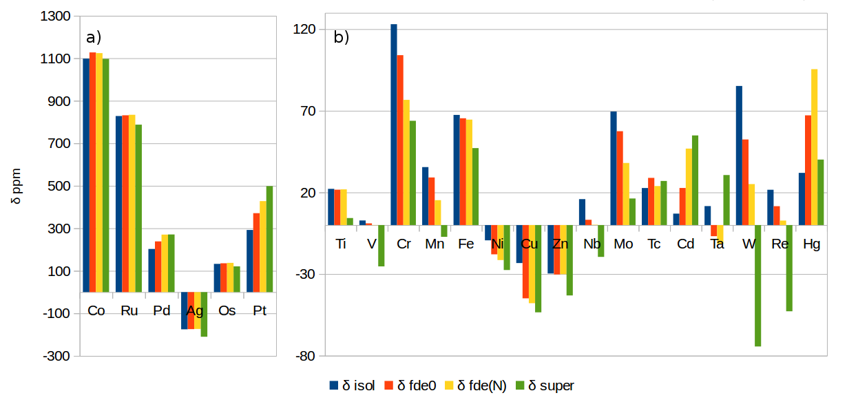
Figure 1: SO-ZORA solvent shifts $\delta_{\text{isol}}$, $\delta_{\text{fde0}}$, $\delta_{\text{fde(N)}}$ and $\delta_{\text{super}}$ calculated for a) systems with $|\delta_{\text{super}}|$ larger than 150 ppm. b) systems with $|\delta_{\text{super}}|$ smaller than 150 ppm.

Comparison of SO-ZORA and DC solvent shifts

Due to the expected cancellation of errors a better agreement between SO-ZORA and DC results is typically obtained for the differences of the absolute shielding constants - for instance for the chemical shifts.[60] This is also observed to some extent for the solvent shifts calculated in this work. As presented in Tables 4 and 5, the overall trends for accurate solvent shifts ($\delta_{\text{super}}$) and for solvent shifts determined by the FDE scheme in fde0 or in fde(N) variants ($\delta_{\text{fde0}}$ and $\delta_{\text{fde(N)}}$, respectively) at the SO-ZORA and DC levels agree rather well. This agreement is not as close as could be expected based on experience with chemical shifts,[60] however, non-negligible differences in the description of solvent effects offered by these two Hamiltonians were already observed in smaller systems with heavy nuclei.[22]

In particular, accurate solvent shifts predicted with these two approaches differ for the studied anionic four-coordinated transition metal oxides in water. In case of heavy 5d transition metals, the SO-ZORA values of $\delta_{\text{super}}$ are significantly larger (in absolute terms) than the DC $\delta_{\text{super}}$ estimates (over 2 times larger in W and Re complexes), while it is the opposite for 3d elements Cr and Mn, in which the absolute values of $\delta_{\text{super}}$ predicted by the SO-ZORA Hamiltonian are smaller than the more accurate four-component values. Among the intermediate 4d elements, the accurate solvent shifts of Mo in MoO${}_{4}^{2-}$ + 12 H₂O are substantially larger when predicted with the SO-ZORA Hamiltonian than when the DC framework is used, while the opposite trend is observed for Ru in Ru(CN)${}_{6}^{4-}$ + 12 H₂O. Other complexes in water do not manifest significant discrepancies of $\delta_{\text{super}}$ values obtained with these two Hamiltonians.

In order to better analyze the FDE results, the SO-ZORA solvent shifts collected in Table 4 are also presented separately for systems with the solvent shifts larger (Figure 1a) and smaller (Figure 1b) than 150 ppm. Taking into account the nature of ’isol’, ’fde0’ and ’fde(N)’ approximations, monotonous convergence of $\delta_{\text{isol}}$, $\delta_{\text{fde0}}$, $\delta_{\text{fde(N)}}$ values towards the reference $\delta_{\text{super}}$ solvent shift is expected. For the systems with largest solvent shifts (Figure 1a), this series of approximations either leads to a systematic improvement of computed solvent shifts (e.g. for PdCl${}_{6}^{2-}$ and PtCl${}_{6}^{2-}$ complexes in water), or results in equally good estimations of these shifts. However, when we consider small solvent shifts we observe a few problematic cases in our test set. For WO${}_{4}^{2-}$ and ReO${}_{4}^{2-}$ complexes in water we find negative reference solvent shifts $\delta_{super}$, whereas the $\delta_{\text{isol}}$, $\delta_{\text{fde0}}$, $\delta_{\text{fde(N)}}$ series of approximations predicts positive solvent shifts, but the trend in the series is correct. A different pattern is observed for Ta(Cl)${}_{6}^{-}$ and Hg(CH₃)₂ systems only, where the sequence of $\delta_{\text{isol}}$, $\delta_{\text{fde0}}$ and $\delta_{\text{fde(N)}}$ does not converge to reference supermolecular shift $\delta_{\text{super}}$.

SO-ZORA $\delta_{\text{fde(N)}}$ predicts the sign of the solvent shift correctly for most complexes in our test set, the most noticeable failures are the W and Re complexes. We recall here that the solvent shift is computed as the difference of two larger numbers (in case of W and Re thousands of ppm), and the performance of the applied approximations for the isolated complex and for the solvated complex may differ. Nevertheless, SO-ZORA $\delta_{\text{fde(N)}}$ approximation predicts the solvent shifts within 20-30 ppm accuracy in most cases.

The DC solvent shifts are presented in Table 5. The monotonous convergence of $\delta_{\text{isol}}$, $\delta_{\text{fde0}}$, $\delta_{\text{fde(N)}}$ values towards the reference $\delta_{\text{super}}$ values is observed only for MnO${}_{4}^{2-}$, Ru(CN)${}_{6}^{4-}$, Pd(Cl)${}_{6}^{2-}$ and Pt(Cl)${}_{6}^{2-}$ complexes. The breakdown of the monotonous behavior in other systems is due to the fact that $\delta_{\text{fde0}}$ values significantly overestimate the reference shifts, yet the correct trend is restored by the fde(N) approach.

For water solvated complexes, DC fde(N) predicts the signs of the solvent shifts consistent with SO-ZORA fde(N) approximation. However, the discrepancy between fde(N) and the corresponding reference supermolecular result, $|\delta_{\text{fde(N)}}$ - $\delta_{\text{super}}|$, is about two times larger for the DC method than for the SO-ZORA method.

Absolute NMR shielding constants are important for the derivation of nuclear magnetic dipole moments [30] from NMR experiments. Therefore, it is instructive to estimate the relative error in absolute shielding constants introduced by different approaches to solvent shifts. In order to analyze the performance of FDE in this context, we define a relative discrepancy $d_{r}$ measured with respect to the solvent-independent absolute value of the shielding in vacuum $|\sigma_{\text{vac}}|$,

$$d_{r}=\frac{\delta-\delta_{\text{super}}}{|\sigma_{\text{vac}}|}=\frac{\sigma-\sigma_{\text{super}}}{|\sigma_{\text{vac}}|},$$ (10)

where $\sigma$ and $\delta$ refer to one of the isol, fde0 and fde(N) models. The relative discrepancies of isol, fde0 and fde(N) approximations for SO-ZORA method are shown in Figure 2a. We note that fairly large $d_{r}$ discrepancies for Cu, Nb and Mo complexes reflect the smallest values of the reference ${|\sigma_{\text{vac}}|}$ for these complexes. In Figure 2b,c, relative discrepancies for SO-ZORA and DC method are compared for the subset of water solvated systems. The calculated average (avg) discrepancy and the standard deviation (std) are shown in Table 6 for the whole set and separately for systems with positive and negative discrepancies, and the largest positive (max) and the largest negative (min) discrepancy is identified. The statistics is calculated separately for SO-ZORA-based results for the complete set of complexes as well as for the SO-ZORA and for the DC results for water solvated systems.

The discrepancy statistics shows that isol, fde0 and fde(N) series of approximations provides an improving description of the solvent effects, toward the reference supermolecular results for all tested subsets except the positive values subset for DC method. However, the statistics of this positive subset for DC method is strongly affected by large discrepancies of Mo complex, which stems from the small value of ${|\sigma_{\text{vac}}|}$. The iterative freeze-and-thaw procedure fde(N) improves noticeably the agreement with the reference supermolecular solvent shifts in comparison to the fde0 procedure. This is mainly due to the capability of fde(N) procedure to reduce the extreme discrepancies (see Figure 2 and Table 6). Generally, all the extreme discrepancies come from the water solvated systems subset, demonstrating that water is a difficult solvent to model. We also note that the improvement within isol, fde0 and fde(N) series of approximations is not guaranteed for every system. Although the extreme discrepancies indicate non-negligible errors in the fde approximations, we find - based on the data of Ref. [30] - that the average and extreme discrepancies between PCM solvent model and supermolecular solvent model in the studied systems reached much larger values (as shown in Table 6).

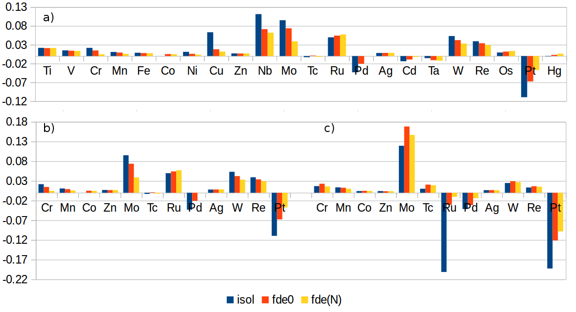
Figure 2: Relative discrepancies between reference $\delta_{\text{super}}$ and $\delta_{\text{isol}}$, $\delta_{\text{fde0}}$ and $\delta_{\text{fde(N)}}$ solvent shifts, calculated using Eq. 10. a) SO-ZORA all systems, b) SO-ZORA water solvated systems, c) DC water solvated systems

Table 6: Discrepancy $d_{r}$ statistics for heavy atoms.

	all $d_{r}$ values			positive $d_{r}$ values				negative $d_{r}$ values
	$avg$	$std$		$avg$	$std$	$max$		$avg$	$std$	$min$
all complexes
SO-ZORA isol	0.016	0.045		0.033	0.033	0.111		-0.029	0.042	-0.109
SO-ZORA fde0	0.013	0.030		0.022	0.023	0.074		-0.027	0.027	-0.068
SO-ZORA fde(N)	0.012	0.022		0.018	0.019	0.062		-0.011	0.016	-0.037
H2O complexes
SO-ZORA isol	0.011	0.051		0.032	0.032	0.095		-0.052	0.053	-0.109
SO-ZORA fde0	0.013	0.036		0.025	0.025	0.074		-0.044	0.033	-0.068
SO-ZORA fde(N)	0.012	0.024		0.021	0.019	0.057		-0.013	0.021	-0.037
DC isol	-0.018	0.091		0.024	0.036	0.119		-0.145	0.090	-0.201
DC fde0	0.009	0.065		0.032	0.052	0.168		-0.061	0.052	-0.121
DC fde(N)	0.011	0.054		0.028	0.045	0.147		-0.041	0.050	-0.098
PCMa	-0.017	0.108		0.162	0.124	0.287		-0.035	0.047	-0.163

^a The discrepancy between PCM and supermolecular solvent shifts, calculated using an analogue of Eq. 10 (based on the data of Ref. [30])

Contributions to solvent effects

More insight into these solvent shifts can be gained from the analysis of different contributions to $\delta$ values. These contributions, measured by the $\Delta$ values defined as

$$\Delta_{\text{isol}} =\sigma_{\text{isol}}-\sigma_{\text{vac}}\equiv\delta_{\text{isol}}$$ (11)

$$\Delta_{\text{fde0}} =\sigma_{\text{fde0}}-\sigma_{\text{isol}}$$ (12)

$$\Delta_{\text{fde(N)}} =\sigma_{\text{fde(N)}}-\sigma_{\text{fde0}}$$ (13)

$$\Delta_{\text{super}} =\sigma_{\text{super}}-\sigma_{\text{fde(N)}}$$ (14)

are summarized in Table 7.

Table 7: Contributions to heavy atom solvent shifts calculated from Eqs. 11-14 with the SO-ZORA and DC Hamiltonians. All values in ppm.

	Solvent	SO-ZORA				DCa
		$\Delta_{\text{isol}}$	$\Delta_{\text{fde0}}$	$\Delta_{\text{fdeN}}$	$\Delta_{\text{super}}$	$\Delta_{\text{isol}}$	$\Delta_{\text{fde0}}$	$\Delta_{\text{fdeN}}$	$\Delta_{\text{super}}$
TiCl4	TiCl4	22.2	-0.5	0.2	-17.6
VOCl3	C6H6	2.8	-1.8	-1.1	-25.2
CrO${}_{4}^{2-}$	H2O	123.0	-19.0	-27.4	-12.8	130.4	17.4	-19.9	-47.4
MnO${}_{4}^{-}$	H2O	35.5	-6.4	-13.9	-22.5	38.0	-3.9	-10.7	-43.3
Fe(CO)5	C6H6	67.4	-2.0	-0.8	-17.5
Co(CN)${}_{6}^{3-}$	H2O	1098.3	29.3	-3.1	-27.1	1158.1	4.0	-2.5	-27.7
Ni(CO)4	C6H6	-9.4	-8.6	-3.5	-6.1
Cu(CH3CN)${}_{4}^{+}$	CH3CN	-23.3	-21.6	-3.0	-5.6
Zn(H2O)${}_{6}^{2+}$	H2O	-29.7	-0.6	0.2	-13.0	-37.7	-0.9	0.1	-7.8
NbCl${}_{6}^{-}$	CH3CN	15.9	-12.7	-3.0	-19.7
MoO${}_{4}^{2-}$	H2O	69.5	-12.0	-19.5	-21.8	67.7	19.8	-8.7	-59.2
TcO${}_{4}^{-}$	H2O	22.7	6.2	-5.0	3.1	22.7	13.2	-2.0	-24.1
Ru(CN)${}_{6}^{4-}$	H2O	828.1	3.6	2.4	-46.4	837.7	130.2	15.3	7.9
PdCl${}_{6}^{2-}$	H2O	202.9	35.7	31.9	0.5	218.0	17.5	31.1	24.5
Ag(H2O)${}_{4}^{+}$	H2O	-175.0	0.8	0.8	-36.7	-181.0	0.2	-0.9	-29.7
Cd(CH3)2	Cd(CH3)2	7.0	15.7	24.1	8.1
TaCl${}_{6}^{-}$	CH3CN	11.6	-18.4	-4.7	42.2
WO${}_{4}^{2-}$	H2O	85.2	-32.8	-27.3	-99.5	78.7	19.9	-9.6	-120.9
ReO${}_{4}^{-}$	H2O	21.6	-10.0	-8.8	-55.6	21.2	11.1	-4.4	-52.2
OsO4	CCl4	132.7	2.8	2.0	-16.4
PtCl${}_{6}^{2-}$	H2O	292.3	78.9	56.9	70.4	327.5	181.9	58.8	251.0
Hg(CH3)2	Hg(CH3)2	32.0	35.2	28.3	-55.4

^a DC results are available only for complexes in water.

The analysis of the $\Delta$ values demonstrates that the solvent shifts in the studied complexes are largely driven by the change of geometry of the solute complexes upon interaction with solvent molecules, with the proportionate contribution of these mechanical effects depending on the Hamiltonian. The relative importance of mechanical and electronic effects may also largely depend on the chosen geometries of these complexes, as previously observed for the MoO${}_{4}^{2-}$ ions in water.[28] Taking the dynamical effects into account – for instance by means of statistical averaging over the range of geometries from molecular dynamics simulations – would then be needed to estimate how these effects interplay in the experimental NMR shielding constants of these complexes in solutions.

In many studied systems the effects not covered by the FDE schemes employed here – measured by $\Delta_{\text{super}}$ – are relatively large. There are many sources of errors that can sum up to $\Delta_{\text{super}}$ values, such as: (i) the neglect of the coupling of responses of subsystems (“uncoupled FDE” approach), (ii) the errors introduced with the selection of the functionals for the non-additive exchange-correlation and the non-additive kinetic energy potentials, and (iii) the use of monomer basis sets.

The lack of intersubsystem coupling at the response level, (i), has two direct consequences. First, it affects the quality of a frozen density – generated without taking into account the response of an active subsystem – which consequently compromises the quality of the embedding potential. Secondly, no information about the response of the environment is included in the response calculations for the active subsystem. To our knowledge, there are no studies that address the errors introduced with this approximation for NMR properties; FDE studies of excitation spectra[61, 62, 63] and chirooptical properties[64] of embedded species indicate that the presence of charge transfer or strong polarization between subsystems requires this coupling to be well described.

In this respect, the quality of the embedding potential is extremely important. Due to the use of approximate exchange-correlation and kinetic energy functionals, (ii), the embedding potential is a local (at best - semilocal) operator, which may not sufficiently well describe the redistribution of the unperturbed densities of an active subsystem and its environment upon interaction. Commonly used functionals for the non-additive kinetic energy potential[24, 65, 66] may introduce artificial low-energy virtual orbitals on the frozen subsystems, in consequence significantly affecting the NMR shielding calculations.[65] The choice of the functionals used for the the non-additive exchange-correlation energy potential can also be relevant. For instance, systems including transition metals may require the use of double-hybrid exchange-correlation functionals,[67] or long-range corrections.[62]

The use of monomer basis sets, (iii), can further compromise the quality of results, because it does not allow for straightforward description of charge transfer between the subsystems. We have performed test calculations on MnO${}_{4}^{-}$ using for each subsystem the supermolecule basis set; we did not pursue this line of inquiry because the small gain in accuracy did not justify the increased computational demands. Typically, the problem is resolved by modifying the partitioning of the total molecular system into subsystems – which might be a sensitive issue in systems involving charged complexes of transition metal atoms. It has been observed that the inclusion of some molecules from the solvent into the active subsystem might be necessary to circumvent the errors introduced with approximations (i)-(iii).[63]

4 Conclusions

We have employed the FDE scheme to calculate solvent shifts of the NMR shielding constants of selected transition metal nuclei in complexes in various solvents. FDE was applied at the relativistic level with the two- and four-component Hamiltonians (SO-ZORA and DC) and with the DFT method used for all subsystems.

In almost every case, for both SO-ZORA and DC Hamiltonians, the fde(N) results are in better agreement with the supermolecular solvent shifts than the fde0 results. Although fde(N) is an iterative procedure, thus more time consuming than fde0, in contrast to the supermolecular approach it still involves only calculations on separate subsystems (which can be performed in their respective basis sets in order to reduce the computational cost - as we have done in this work). Moreover, the fde(N) procedure was found to converge fast (the changes in the total energies in two last freeze-and-thaw iterations are lower than 1e-06 a.u.), thus qualitatively correct results could be obtained in smaller number of freeze-and-thaw iterations.

In comparison with recently published PCM results on the same systems,[30] FDE values seem to be more reliable overall - the dispersion of FDE solvent shifts in the studied set is significantly lower than the one based on PCM values. Qualitatively, both models agree in most cases by predicting the same signs of solvent shifts, yet neither is accurate in all studied systems. With these studies we therefore hope to encourage further tests of the FDE scheme on NMR properties, in order to understand its applicability in various complex systems and direct its further developments.

Accompanying supermolecular calculations (at the same relativistic DFT levels) allowed to assess the accuracy of the FDE approach. We found that FDE in its canonical formulation does not guarantee satisfactory results, even when the role of subsystems is repeatedly interchanged in the freeze-and-thaw procedure leading to self-consistently optimized electron densities of subsystems. The electronic contributions to solvent shifts cannot be neglected, even when a significant portion of the solvent shifts is actually recovered by mechanical solvent effects – the latter governed by the relaxation of subsystems’ geometries in the formation of the supermolecule. This calls for a better description and analysis of these electronic effects on the shifts, one that goes beyond the fde(N) approach. Another interesting dilemma are the differences between solvent shifts at the SO-ZORA and DC levels, which emphasize that one should not rely on the cancellation of errors when calculating solvent shifts to the same degree as in the evaluation of the NMR chemical shifts. Recalling that NMR properties depend on the magnetic-field induced currents, which may encompass the whole supermolecule, a "coupled-FDE" approach in which each subsystem interacts with the other, with both simultaneously perturbed by the external field, appears to be an extension worth exploring. Considering the number of approximations in our work (such as the use of DFT and monomer basis sets) the improved performance of fde(N) with respect to fde0 successfully confirms the advantages of the FDE approach.

Research Resources

This research was supported in part by PLGrid Infrastructure.

Conflict of interest

There are no conflicts to declare.

Data Accessibility

The data that support the findings of this study (inputs and outputs of calculations) are openly available in Zenodo at DOI: 10.5281/zenodo.4883729

References

- [1] M. Kaupp, M. Buhl, and V. G. Malkin, Calculation of NMR and EPR Parameters: Theory and Applications; Wiley-VCH, 2004.
- [2] J. Autschbach, Phil. Trans. R. Soc. A, 2014, 372, 20120489.
- [3] M. Kaupp; Relativistic Effects on NMR Chemical Shifts; In P. Schwerdtfeger, Eds., Relativistic Electronic Structure Theory. Part 2. Applications, pages 552–597, Amsterdam, 2004. Elsevier.
- [4] J. Autschbach; Relativistic Effects on Magnetic Resonance Parameters and Other Properties of Inorganic Molecules and Metal Complexes; In M. Barysz and Y. Ishikawa, Eds., Relativistic Methods for Chemists, pages 521–598. Springer, Dordrecht, 2010.
- [5] A. Antušek and M. Jaszuński; Accurate Nonrelativistic Calculations of NMR Shielding Constants; In K. Jackowski and M. Jaszuński, Ed., Gas Phase NMR, pages 186–217. The Royal Society of Chemistry, 2016.
- [6] M. Repisky, S. Komorovsky, R. Bast, and K. Ruud; Relativistic Calculations of Nuclear Magnetic Resonance Parameters; In K. Jackowski and M. Jaszuński, Ed., Gas Phase NMR, chapter 8, pages 267–303. The Royal Society of Chemistry, 2016.
- [7] J. Tomasi, B. Mennucci, and R. Cammi, Chem. Rev., 2005, 105, 2999–3094.
- [8] R. Di Remigio, R. Bast, L. Frediani, and T. Saue, J. Phys. Chem. A, 2015, 119, 5061–5077.
- [9] A. Fortunelli and J. Tomasi, Chem. Phys. Lett., 1994, 231, 34–39.
- [10] R. Di Remigio, A. H. Steindal, K. Mozgawa, V. Weijo, H. Cao, and L. Frediani, Int. J. Quantum Chem., 2018, 119, e25685.
- [11] A. Klamt and G. Schüürmann, J. Chem. Soc., Perkin Trans. 2, 1993, pages 799–805.
- [12] C. R. Jacob and L. Visscher, J. Chem. Phys., 2006, 125, 194104.
- [13] B. Mennucci, J. M. Martínez, and J. Tomasi, J. Phys. Chem. A, 2001, 105, 7287–7296.
- [14] C. Steinmann, J. M. H. Olsen, and J. Kongsted, J. Chem. Theory Comp., 2014, 10, 981–988.
- [15] C. Steinmann, L. A. Bratholm, J. M. H. Olsen, and J. Kongsted, J. Chem. Theory Comp., 2017, 13, 525–536.
- [16] G. Senatore and K. R. Subbaswamy, Phys. Rev. B, 1986, 34, 5754–5757.
- [17] P. Cortona, Phys. Rev. B, 1991, 44, 8454–8458.
- [18] T. A. Wesolowski and A. Warshel, J. Phys. Chem., 1993, 97, 8050–8053.
- [19] A. Krishtal, D. Sinha, A. Genova, and M. Pavanello, J. Phys.: Condens. Matter, 2015, 27, 183202.
- [20] R. E. Bulo, C. R. Jacob, and L. Visscher, J. Phys. Chem. A, 2008, 112, 2640–2647.
- [21] A. W. Götz, J. Autschbach, and L. Visscher, J. Chem. Phys., 2014, 140, 104107.
- [22] M. Olejniczak, R. Bast, and A. S. Pereira Gomes, Phys. Chem. Chem. Phys., 2017, 19, 8400–8415.
- [23] A. S. P. Gomes and C. R. Jacob, Annu. Rep. Prog. Chem., Sect. C: Phys. Chem., 2012, 108, 222–277.
- [24] C. R. Jacob and J. Neugebauer, Wiley Interdiscip. Rev. Comput. Mol. Sci., 2014, 4, 325–362.
- [25] T. A. Wesolowski, S. Shedge, and X. Zhou, Chem. Rev., 2015, 115, 5891–5928.
- [26] Q. Sun and G. K. L. Chan, Acc. Chem. Res., 2016, 49, 2705–2712.
- [27] L. O. Jones, M. A. Mosquera, G. C. Schatz, and M. A. Ratner, J. Am. Chem. Soc., 2020, 142, 3281–3295.
- [28] L. Halbert, M. Olejniczak, V. Vallet, and A. S. P. Gomes, Int. J. Quantum Chem., 2020, 120, e26207.
- [29] R. K. Harris, E. D. Becker, S. M. C. de Menezes, R. Goodfellow, and P. Granger, Pure Appl. Chem, 2001, 73, 1795–1818, reprinted in Magn. Reson. in Chem. 40 (2002) 489–505.
- [30] A. Antušek and M. Repisky, Phys. Chem. Chem. Phys., 2020, 22, 7065–7076.
- [31] R. Bast, H. J. Aa. Jensen, and T. Saue, Int. J. Quantum Chem., 2009, 109, 2091–2112.
- [32] S. Komorovský, M. Repiský, O. L. Malkina, V. G. Malkin, I. Malkin Ondík, and M. Kaupp, J. Chem. Phys., 2008, 128, 104101.
- [33] M. Olejniczak, R. Bast, T. Saue, and M. Pecul, J. Chem. Phys., 2012, 136, 014108, Erratum: ibid. 136, 239902, (2012).
- [34] T. A. Wesolowski and J. Weber, Chem. Phys. Lett., 1996, 248, 71–76.
- [35] M. E. Casida and T. A. Wesolowski, Int. J. Quantum Chem., 2004, 96, 577–588.
- [36] J. Neugebauer, J. Chem. Phys., 2007, 126, 134116.
- [37] J. Neugebauer, J. Chem. Phys., 2009, 131, 084104.
- [38] S. Höfener, A. S. P. Gomes, and L. Visscher, J. Chem. Phys., 2012, 136, 044104.
- [39] P. v. R. Schleyer, C. Maerker, A. Dransfeld, H. Jiao, and N. J. R. v. E. Hommes, J. Am. Chem. Soc., 1996, 118, 6317–6318.
- [40] C. Adamo and V. Barone, J. Chem. Phys., 1999, 110, 6158–6170.
- [41] F. Weigend and R. Ahlrichs, Phys. Chem. Chem. Phys., 2005, 7, 3297–3305.
- [42] E. van Lenthe, E. J. Baerends, and J. G. Snijders, J. Chem. Phys., 1993, 99, 4597–4610.
- [43] E. van Lenthe, E. J. Baerends, and J. G. Snijders, J. Chem. Phys., 1994, 101, 9783–9792.
- [44] G. te Velde, F. M. Bickelhaupt, E. J. Baerends, C. Fonseca Guerra, S. J. A. van Gisbergen, J. G. Snijders, and T. Ziegler, J. Comput. Chem., 2001, 22, 931–967.
- [45] ADF 2019.3, SCM, Theoretical Chemistry, Vrije Universiteit, Amsterdam, The Netherlands, http://www.scm.com.
- [46] C. R. Jacob, S. M. Beyhan, R. E. Bulo, A. S. P. Gomes, A. W. Götz, K. Kiewisch, J. Sikkema, and L. Visscher, J. Comput. Chem., 2011, 32, 2328–2338.
- [47] T. Saue, R. Bast, A. S. P. Gomes, H. J. Aa. Jensen, L. Visscher, I. A. Aucar, R. Di Remigio, K. G. Dyall, E. Eliav, E. Faßhauer, T. Fleig, L. Halbert, E. D. Hedegård, B. Heimlich-Paris, M. Iliaš, Ch. R. Jacob, S. Knecht, J. K. Lærdahl, M. L. Vidal, M. K. Nayak, M. Olejniczak, J. M. H. Olsen, M. Pernpointner, B. Senjean, A. Shee, A. Sunaga, and J. van Stralen, J. Chem. Phys., 2020, 152, 204104.
- [48] DIRAC, a relativistic ab initio electronic structure program, Release DIRAC19 (2019), written by A. S. P. Gomes, T. Saue, L. Visscher, H. J. Aa. Jensen, and R. Bast, with contributions from I. A. Aucar, V. Bakken, K. G. Dyall, S. Dubillard, U. Ekström, E. Eliav, T. Enevoldsen, E. Faßhauer, T. Fleig, O. Fossgaard, L. Halbert, E. D. Hedegård, B. Heimlich–Paris, T. Helgaker, J. Henriksson, M. Iliaš, Ch. R. Jacob, S. Knecht, S. Komorovský, O. Kullie, J. K. Lærdahl, C. V. Larsen, Y. S. Lee, H. S. Nataraj, M. K. Nayak, P. Norman, G. Olejniczak, J. Olsen, J. M. H. Olsen, Y. C. Park, J. K. Pedersen, M. Pernpointner, R. di Remigio, K. Ruud, P. Sałek, B. Schimmelpfennig, B. Senjean, A. Shee, J. Sikkema, A. J. Thorvaldsen, J. Thyssen, J. van Stralen, M. L. Vidal, S. Villaume, O. Visser, T. Winther, and S. Yamamoto (available at http://dx.doi.org/10.5281/zenodo.3572669, see also http://www.diracprogram.org).
- [49] B. O. Roos, R. Lindh, P.-Å. Malmqvist, V. Veryazov, and P.-O. Widmark, J. Phys. Chem. A, 2004, 108, 2851–2858.
- [50] T. H. Dunning Jr., J. Chem. Phys., 1989, 90, 1007–1023.
- [51] L. Visscher, Theor. Chem. Acc., 1997, 98, 68–70.
- [52] A. D. Becke, J. Chem. Phys., 1993, 98, 5648–5652.
- [53] A. D. Becke, Phys. Rev. A, 1988, 38, 3098–3100.
- [54] C. Lee, W. Yang, and R. G. Parr, Phys. Rev. B, 1988, 37, 785–789.
- [55] A. Lembarki and H. Chermette, Phys. Rev. A, 1994, 50, 5328–5331.
- [56] A. W. Götz, S. Maya Beyhan, and L. Visscher, J. Chem. Theory Comput., 2009, 5, 3161–3174.
- [57] F. London, J. Phys. Radium, 1937, 8, 397–409.
- [58] K. Wolinski, J. F. Hinton, and P. Pulay, J. Am. Chem. Soc., 1990, 112, 8251–8260.
- [59] J. Neugebauer, Ch. R. Jacob, T. A. Wesolowski, and E. J. Baerends, J. Phys. Chem. A, 2005, 109, 7805–7814.
- [60] J. Autschbach, Mol. Phys., 2013, 111, 2544–2554.
- [61] N. Ricardi, A. Zech, Y. Gimbal-Zofka, and T. A Wesołowski, Phys. Chem. Chem. Phys., 2018, 20, 26053–26062.
- [62] J. Tölle, M. Böckers, N. Niemeyer, and J. Neugebauer, J. Chem. Phys., 2019, 151, 174109.
- [63] L. Scholz, J. Tölle, and J. Neugebauer, Int. J. Quantum Chem., 2020, 120, e26213.
- [64] N. Niemeyer, J. Tölle, and J. Neugebauer, J. Chem. Theory Comput., 2020, 16, 3104–3120.
- [65] C. R. Jacob, S. M. Beyhan, and L. Visscher, J. Chem. Phys., 2007, 126, 234116.
- [66] M. Banafsheh and T.A. Wesolowski, Int. J. Quantum Chem., 2018, 118, e25410.
- [67] M. Bensberg and J. Neugebauer, Phys. Chem. Chem. Phys., 2020, 22, 26093–26103.