Motif Prediction with Graph Neural Networks

Abstract.

Link prediction is one of the central problems in graph mining. However, recent studies highlight the importance of higher-order network analysis, where complex structures called motifs are the first-class citizens. We first show that existing link prediction schemes fail to effectively predict motifs. To alleviate this, we establish a general motif prediction problem and we propose several heuristics that assess the chances for a specified motif to appear. To make the scores realistic, our heuristics consider – among others – correlations between links, i.e., the potential impact of some arriving links on the appearance of other links in a given motif. Finally, for highest accuracy, we develop a graph neural network (GNN) architecture for motif prediction. Our architecture offers vertex features and sampling schemes that capture the rich structural properties of motifs. While our heuristics are fast and do not need any training, GNNs ensure highest accuracy of predicting motifs, both for dense (e.g., $k$-cliques) and for sparse ones (e.g., $k$-stars). We consistently outperform the best available competitor by more than 10% on average and up to 32% in area under the curve. Importantly, the advantages of our approach over schemes based on uncorrelated link prediction increase with the increasing motif size and complexity. We also successfully apply our architecture for predicting more arbitrary clusters and communities, illustrating its potential for graph mining beyond motif analysis.

1. Introduction and Motivation

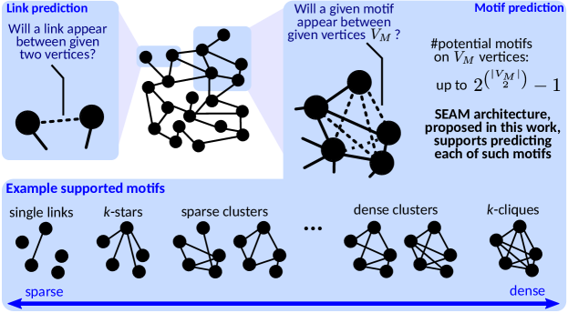
One of the central problems in graph mining and learning is link prediction (lu2011link, ; al2006link, ; taskar2004link, ; al2011survey, ; zhang2018link, ; zhang2020revisiting, ), in which one is interested in assessing the likelihood that a given pair of vertices is, or may become, connected. However, recent works argue the importance of higher-order graph organization (benson2016higher, ), where one focuses on finding and analyzing small recurring subgraphs called motifs (sometimes referred to as graphlets or graph patterns) instead of individual links. Motifs are central to many graph mining problems in computational biology, chemistry, and a plethora of other fields (besta2021graphminesuite, ; besta2021sisa, ; cook2006mining, ; jiang2013survey, ; horvath2004cyclic, ; chakrabarti2006graph, ; besta2019slim, ). Specifically, motifs are building blocks of different networks, including transcriptional regulation graphs, social networks, brain graphs, or air traffic patterns (benson2016higher, ). There exist many motifs, for example $k$-cliques, $k$-stars, $k$-clique-stars, $k$-cores, and others (lee2010survey, ; jabbour2018pushing, ; besta2017push, ). For example, cliques or quasi-cliques are crucial motifs in protein-protein interaction networks (bhattacharyya2009mining, ; li2005interaction, ). A huge number of works are dedicated to motif counting, listing (also called enumeration), or checking for the existence of a given motif (besta2021graphminesuite, ; cook2006mining, ). However, while a few recent schemes focus on predicting triangles (benson2018simplicial, ; nassar2020neighborhood, ; nassar2019pairwise, ), no works target the problem of general motif prediction, i.e., analyzing whether specified complex structures may appear in the data. As with link prediction, it would enable predicting the evolution of data, but also finding missing structures in the available data. For example, one could use motif prediction to find probable missing clusters of interactions in biological (e.g., protein) networks, and use the outcomes to limit the number of expensive experiments conducted to find missing connections (lu2011link, ; martinez2016survey, ).

In this paper, we first (Section 3) establish and formally describe a general motif prediction problem, going beyond link prediction and showing how to predict higher-order network patterns that will appear in the future (or which may be missing from the data). A key challenge is the appropriate problem formulation. Similarly to link prediction, one wants a score function that – for a given vertex set $V_{M}$ – assesses the chances for a given motif to appear. Still, the function must consider the combinatorially increased complexity of the problem (compared to link prediction). In general, contrary to a single link, a motif may be formed by an arbitrary set $V_{M}$ of vertices, and the number of potential edges between these vertices can be large, i.e., $O(|V_{M}|^{2})$. For example, one may be interested in analyzing whether a group of entities $V_{M}$ may become a $k$-clique in the future, or whether a specific vertex $v\in V_{M}$ will become a hub of a $k$-star, connecting $v$ to $k-1$ other selected vertices from $V_{M}\setminus\{v\}$. This leads to novel issues, not present in link prediction. For example, what if some edges, belonging to the motif being predicted, already exist? How should they be treated by a score function? Or, how to enable users to apply their domain knowledge? For example, when predicting whether the given vertices will form some chemical particle, a user may know that the presence of some link (e.g., some specific atomic bond) may increase (or decrease) the chances for forming another bond. Now, how could this knowledge be provided in the motif score function? We formally specify these and other aspects of the problem in a general theoretical framework, and we provide example motif score functions. We explicitly consider correlations between edges forming a motif, i.e., the fact that the appearance of some edges may increase or decrease the overall chances of a given motif to appear.

Figure 1. Motivating our work (SEAM): the accuracy (%) of predicting different motifs with SEAM compared to using a state-of-the-art SEAL link prediction scheme (zhang2018link, ; zhang2020revisiting, ) and a naive one that does not consider correlations between edges. The details of the experimental setup are in Section 5 (the dataset is USAir). Importantly: (1) SEAM outperforms all other methods, (2) the accuracy of SEAM increases with the size ($k$) of each motif, while in other methods it decreases.

Then, we develop a learning architecture based on graph neural networks (GNNs) to further enhance motif prediction accuracy (Section 4). For this, we extend the state-of-the-art SEAL link prediction framework (zhang2018link, ) to support arbitrary motifs. For a given motif $M$, we train our architecture on what is the “right motif surroundings” (i.e., nearby vertices and edges) that could result in the appearance of $M$. Then, for a given set of vertices $V_{M}$, the architecture infers the chances for $M$ to appear. The key challenge is to be able to capture the richness of different motifs and their surroundings. We tackle this with an appropriate selection of negative samples, i.e., subgraphs that resemble the searched motifs but that are not identical to them. Moreover, when selecting the size of the “motif surroundings” we rely on an assumption also used in link prediction, which states that only the “close surroundings” (i.e., nearby vertices and edges, 1–2 hops away) of a link to be predicted have a significant impact on whether or not this link would appear (zhang2018link, ; zhang2020revisiting, ). We use this assumption for motifs: as our evaluation shows, it ensures high accuracy while significantly reducing runtimes of training and inference (as only a small subgraph is used, instead of the whole input graph). We call our GNN architecture SEAM: learning from Subgraphs, Embeddings and Attributes for Motif prediction. Our evaluation (Section 5) illustrates the high accuracy of SEAM (often more than 90%), for a variety of graph datasets and motif sizes.

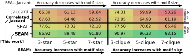
To motivate our work, we now compare SEAM and a proposed Jaccard-based heuristic that considers link correlations to two baselines that straightforwardly use link prediction independently for each motif link: a Jaccard-based score and the state-of-the-art SEAL scheme based on GNNs (zhang2018link, ). We show the results in Figure 1. The correlated Jaccard outperforms a simple Jaccard, while the proposed SEAM is better than SEAL. The benefits generalize to different graph datasets. Importantly, we observe that the larger the motif to predict becomes (larger $k$), the more advantages our architecture delivers. This is because larger motifs provide more room for correlations between their associated edges. Straightforward link prediction based schemes do not consider this effect, while our methods do, which is why we offer more benefits for more complex motifs. The advantages of SEAM over the correlated Jaccard show that GNNs more robustly capture correlations and the structural richness of motifs than simple manual heuristics. Simultaneously, heuristics do not need any training. Finally, SEAM also successfully predicts more arbitrary communities or clusters (lee2010survey, ; gibson2005discovering, ; besta2021graphminesuite, ; besta2021sisa, ). They differ from motifs as they do not have a very specific fixed structure (such as a star) but simply have the edge density above a certain threshold. SEAM’s high accuracy in predicting such structures illustrates its potential for broader graph mining beyond motif analysis.

Overall, the key contributions of our paper are (1) identifying and formulating the motif prediction problem and the associated score functions, (2) showing how to solve this problem with heuristics and graph neural networks, and (3) illustrating that graph neural networks can solve this problem more effectively than heuristics.

2. Background and Notation

We first describe the necessary background and notation.

Graph Model We model an undirected graph $G$ as a tuple $(V,E)$; $V$ and $E\subseteq V\times V$ are sets of nodes (vertices) and links (edges); $|V|=n$, $|E|=m$. Vertices are modeled with integers $1,...,n$; $V=\{1,...,n\}$. $N_{v}$ denotes the neighbors of $v\in V$; $d(v)$ denotes the degree of $v$.

Link Prediction We generalize the well-known link prediction problem. Consider two unconnected vertices $u$ and $v$. We assign a similarity score $s_{u,v}$ to them. All pairs of vertices that are not edges receive such a score and are ranked according to it. The higher a similarity score is, the “more likely” a given edge is to be missing in the data or to be created in the future. We stress that the link prediction scores are usually not based on any probabilistic notion (in the formal sense) and are only used to make comparisons between pairs of vertices in the same input graph dataset.

There are numerous known similarity scores. First, a large number of scores are called first order because they only consider the neighbors of $u$ and $v$ when computing $s_{u,v}$. Examples are the Common Neighbors scheme $s_{u,v}^{CN}=\lvert N_{u}\cap N_{v}\rvert$ or the Jaccard scheme $s_{u,v}^{J}=\frac{\lvert N_{u}\cap N_{v}\rvert}{\lvert N_{u}\cup N_{v}\rvert}$ (besta2020communication, ). These schemes assume that two vertices are more likely to be linked if they have many common neighbors. There also exist similarity schemes that consider vertices not directly attached to $u$ and $v$. All these schemes can be described using the same formalism of the $\gamma$-decaying heuristic proposed by (zhang2018link, ). Intuitively, for a given pair of vertices $(u,v)$, the $\gamma$-decaying heuristic for $(u,v)$ provides a sum of contributions into the link prediction score for $(u,v)$ from all other vertices, weighted in such a way that nearby vertices have more impact on the score.

Graph Neural Networks Graph neural networks (GNNs) are a recent class of neural networks for learning over irregular data such as graphs (scarselli2008graph, ; zhang2019heterogeneous, ; zhou2020graph, ; thekumparampil2018attention, ; wu2020comprehensive, ; sato2020survey, ; wu2020graph, ; zhang2020deep, ; chen2020bridging, ; cao2020comprehensive, ). There exists a plethora of models and methods for GNNs; most of them consist of two fundamental parts: (1) an aggregation layer that combines the features of the neighbors of each node, for all the nodes in the input graph, and (2) combining the scores into a new score. The input to a GNN is a tuple $G=(A,X)$. The input graph $G$ having $n$ vertices is modeled with an adjacency matrix $A\in\mathbb{R}^{n\times n}$. The features of vertices (with dimension $d$) are modeled with a matrix $X\in\mathbb{R}^{n\times d}$.

Figure 2. Illustration of the motif prediction problem and example supported motifs. We provide support for predicting arbitrary motifs.

Symbol	Description
$E_{M}$	All edges forming a motif in question; $E_{M}=E_{M,\mathcal{N}}\cup E_{M,\mathcal{E}}$
$E_{M,\mathcal{N}}$	Motif edges that do not yet exist
$E_{M,\mathcal{E}}$	Motif edges that already exist in the data
$\overline{E}_{M}$	Edges not in $E_{M}$, defined over vertex pairs in $V_{M}$; $\overline{E}_{M}=\overline{E}_{M,\mathcal{D}}\cup\overline{E}_{M,\mathcal{I}}$
$E_{V_{M}}$	All possible edges between motif vertices; $E_{V_{M}}=\overline{E}_{M}\cup E_{M}$
$\overline{E}_{M,\mathcal{D}}$	Deal-breaker edges; $\overline{E}_{M,\mathcal{D}}=\overline{E}_{M,\mathcal{D},\mathcal{N}}\cup\overline{E}_{M,\mathcal{D},\mathcal{E}}$
$\overline{E}_{M,\mathcal{D},\mathcal{N}}$	Deal-breaker edges that do not exist yet
$\overline{E}_{M,\mathcal{D},\mathcal{E}}$	Deal-breaker edges that already exist
$\overline{E}_{M,\mathcal{I}}$	Non deal-breaker edges in $\overline{E}_{M}$; “edges that do not matter”
$E^{*}_{M}$	“Edges that matter for the score”: $E^{*}_{M}=E_{M}\cup\overline{E}_{M,\mathcal{D}}$
$E^{*}_{M,\mathcal{E}}$	All existing edges “that matter”: $E^{*}_{M,\mathcal{E}}=E_{M,\mathcal{E}}\cup\overline{E}_{M,\mathcal{D},\mathcal{E}}$
$E^{*}_{M,\mathcal{N}}$	All non-existing edges “that matter”: $E^{*}_{M,\mathcal{N}}=E_{M,\mathcal{N}}\cup\overline{E}_{M,\mathcal{D},\mathcal{N}}$

Table 1. Different types of edges used in this work.

3. Motif Prediction: Formal Statement and Score Functions

We now formally establish the motif prediction problem. We define a motif as a pair $M=(V_{M},E_{M})$. $V_{M}$ is the set of existing vertices of $G$ that form a given motif ($V_{M}\subseteq V$). $E_{M}$ is the set of edges of $G$ that form the motif being predicted; some of these edges may already exist ($E_{M}\subseteq V_{M}\times V_{M}$).

We make the problem formulation (in § 3.1–§ 3.3) general: it can be applied to any graph generation process. Using this formulation, one can then devise specific heuristics that may assume some details on how the links are created, similarly as is done in link prediction. Here, we propose example motif prediction heuristics that harness the Jaccard, Common Neighbors, and Adamic-Adar link scores.

We illustrate motif prediction problem and example supported motifs in Figure 2.

3.1. Motif Prediction vs. Link Prediction

We illustrate the motif prediction problem by discussing the differences between link and motif prediction. We consider all these differences when proposing specific schemes for predicting motifs.

(M) There May Be Many Potential New Motifs For a Fixed Vertex Set  Link prediction is a “binary” problem: for a given pair of unconnected vertices, there can only be one link appearing. In motif prediction, the situation is more complex. There are many possible motifs to appear between given vertices $v_{1},...,v_{k}$. We now state a precise count; the proof is in the appendix.

Observation 1.

Consider vertices $v_{1},...,v_{k}\in V$. Assuming no edges already connecting $v_{1},...,v_{k}$, there are $2^{\binom{k}{2}}-1$ motifs (with between 1 and $\binom{k}{2}$ edges) that can appear to connect $v_{1},...,v_{k}$.

Note that this is the largest possible number, which assumes no previously existing edges, and permutation dependence, i.e., two motifs that are isomorphic but have different vertex orderings, are treated as two different motifs. This enables, for example, the user to be able to distinguish between two stars rooted at different vertices. This is useful in, e.g., social network analysis, when stars rooted at different persons may well have different meaning.

(E) There May Be Existing Edges A link can only appear between unconnected vertices. Contrarily, a motif can appear and connect vertices already with some edges between them.

(D) There May Be “Deal-Breaker” Edges There may be some edges, the appearance of which would make the appearance of a given motif unlikely or even impossible (e.g., existing chemical bonds could prevent other bonds). For example, consider a prediction query where one is interested whether a given vertex set can become connected with a star but in such a way that none of the non-central vertices are connected to one another. Now, if there is already some edge connecting these non-central vertices, this makes it impossible a given motif to appear while satisfying the query. We will refer to such edges as the “deal-breaker” edges.

(L) Motif Prediction Query May Depend on Vertex Labeling The query can depend on a specific vertex labeling. For example, when asking whether a 5-star will connect six given vertices $v_{1},...,v_{6}$, one may be interested in any 5-star connecting $v_{1},...,v_{6}$, or a 5-star connecting these vertices in a specific way, e.g., with its center being $v_{1}$. We enable the user to specify how edges in $E_{M}$ should connect vertices in $V_{M}$.

3.2. Types of Edges in Motifs

Figure 3. Illustration of edge types in motif prediction.

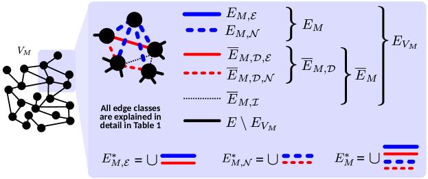
We first describe different types of edges related to a motif. They are listed in Table 1 and shown in Figure 3. First, note that motif edges $E_{M}$ are a union of two types of motif edges, i.e., $E_{M}=E_{M,\mathcal{N}}\cup E_{M,\mathcal{E}}$ where $E_{M,\mathcal{N}}$ are edges that do not exist in $G$ at the moment of querying ($\forall_{e\in E_{M,\mathcal{N}}}e\not\in E$; $\mathcal{N}$ indicates “$\mathcal{N}$on-existing”) and $E_{M,\mathcal{E}}$ are edges that already exist, cf. (E) in § 3.1 ($\forall_{e\in E_{M,\mathcal{E}}}e\in E$; $\mathcal{E}$ indicates “$\mathcal{E}$xisting”). Moreover, there may be edges between vertices in $V_{M}$ which do not belong to $M$ (i.e., they belong to $E_{V_{M}}=\{\{i,j\}:i,j\in V_{M}\land i\neq j\}$ but not $E_{M}$). We refer to such edges as $\overline{E}_{M}$ since $E_{V_{M}}=\overline{E}_{M}\cup E_{M}$ (i.e., a union of disjoints sets). Some edges in $\overline{E}_{M}$ may be deal-breakers (cf. (D) in § 3.1), we denote them as $\overline{E}_{M,\mathcal{D}}$ ($\mathcal{D}$ indicates “$\mathcal{D}$eal-breaker”). Non deal-breakers that are in $\overline{E}_{M}$ are denoted with $\overline{E}_{M,\mathcal{I}}$ ($\mathcal{I}$ indicates “$\mathcal{I}$nert”). Note that $\overline{E}_{M}=\overline{E}_{M,\mathcal{D}}\cup\overline{E}_{M,\mathcal{I}}$ and $\overline{E}_{M}=E_{V_{M}}\setminus E_{M}$. To conclude, as previously done for the set $E_{M}$, we note that $\overline{E}_{M,\mathcal{D}}=\overline{E}_{M,\mathcal{D},\mathcal{N}}\cup\overline{E}_{M,\mathcal{D},\mathcal{E}}$ where $\overline{E}_{M,\mathcal{D},\mathcal{N}}$ are deal-breaker edges that do not exist in $G$ at the moment of querying ($\forall_{e\in\overline{E}_{M,\mathcal{D},\mathcal{N}}}e\not\in E$; $\mathcal{N}$ indicates “$\mathcal{N}$on-existing”) and $\overline{E}_{M,\mathcal{D},\mathcal{E}}$ are deal-breaker edges that already exist, cf. (E) in § 3.1 ($\forall_{e\in\overline{E}_{M,\mathcal{D},\mathcal{E}}}e\in E$; $\mathcal{E}$ indicates “$\mathcal{E}$xisting”). We explicitly consider $\overline{E}_{M,\mathcal{D},\mathcal{N}}$ because – even if a given deal-breaker edge does not exist, but it does have a large chance of appearing – the motif score should become lower.

3.3. General Problem and Score Formulation

We now formulate a general motif prediction score. Analogously to link prediction, we assign scores to motifs, to be able to quantitatively assess which motifs are more likely to occur. Thus, one obtains a tool for analyzing future (or missing) graph structure, by being able to quantitatively compare different ways in which vertex sets may become (or already are) connected. Intuitively, we assume that a motif score should be high if the scores of participating edges are also high. This suggests one could reuse link prediction score functions. Full extensive details of score functions, as well as more examples, are in the appendix.

A specific motif score function $s(M)$ will heavily depend on a targeted problem. In general, we define $s(M)$ as a function of $V_{M}$ and $E^{*}_{M}$; $s(M)=s(V_{M},E^{*}_{M})$. Here, $E^{*}_{M}=E_{M}\cup\overline{E}_{M,\mathcal{D}}$ are all the edges “that matter”: both edges in a motif ($E_{M}$) and the deal-breaker edges ($\overline{E}_{M,\mathcal{D}}$). To obtain the exact form of $s(M)$, we harness existing link prediction scores for edges from $E_{M}$, when deriving $s(M)$ (details in § 3.4–§ 3.5). When using first-order link prediction methods (e.g., Jaccard), $s(M)$ depends on $V_{M}$ and potential direct neighbors. With higher-order methods (e.g., Katz (katz1953new, ) or Adamic-Adar (adamic2003friends, )), a larger part of the graph that is “around $V_{M}$” is considered for computing $s(M)$. Here, our evaluation (cf. Section 5) shows that, similarly to link prediction (zhang2018link, ), it is enough to consider a small part of $G$ (1-2 hops away from $V_{M}$) to achieve high prediction accuracy for motifs.

Still, simply extending link prediction fails to account for possible correlations between edges forming the motif (i.e., edges in $E_{M}$). Specifically, the appearance of some edges may impact (positively or negatively) the chances of one or more other edges in $E_{M}$. We provide score functions that consider such correlations in § 3.5.

3.4. Heuristics with No Link Correlations

There exist many score functions for link prediction (lu2011link, ; al2006link, ; taskar2004link, ; al2011survey, ). Similarly, one can develop motif prediction score functions with different applications in mind. As an example, we discuss score functions for a graph that models a set of people. An edge between two vertices indicates that two given persons know each other. For simplicity, let us first assume that there are no deal-breaker edges, thus $E^{*}_{M}=E_{M}$. For a set of people $V_{M}$, we set the score of a given specific motif $M=(V_{M},E_{M})$ to be the product of the scores of the associated edges: $s_{\perp}(M)=\prod_{e\in E_{M,\mathcal{N}}}s(e)$ where $\perp$ denotes the independent aggregation scheme. Here, $s(e)$ is any link prediction score which outputs into $[0,1]$ (e.g., Jaccard). Thus, also $s_{\perp}(M)\in[0,1]$ by construction. Moreover, this score implicitly states that $\forall e\in E_{M,\mathcal{E}}$ we set $s(e)=1$. Clearly, this does not impact the motif score $s_{\perp}(M)$ as the edges are already $\mathcal{E}$xisting. Overall, we assume that a motif is more likely to appear if the edges that participate in that motif are also more likely. Now, when using the Jaccard Score for edges, the motif prediction score becomes $s_{\perp}(M)^{J}=\prod_{e_{u,v}\in E_{M,\mathcal{N}}}\frac{\lvert N_{u}\cap N_{v}\rvert}{\lvert N_{u}\cup N_{v}\rvert}$.

To incorporate deal-breaker edges, we generalize the motif score defined previously as $s_{\perp}^{*}(M)=\prod_{e\in E_{M}}{s(e)}\cdot\prod_{e\in\overline{E}_{M,\mathcal{D}}}\left(1-{s(e)}\right)$, where the product over $E_{M}$ includes partial scores from the edges that belong to the motif, while the product over $\overline{E}_{M,\mathcal{D}}$ includes the scores from deal-breaker edges. Here, the larger the chance for a $e$ to appear, the higher its score $s(e)$ is. Thus, whenever $e$ is a deal-breaker, using $1-s(e)$ has the desired diminishing effect on the final motif score $s_{\perp}^{*}(M)$.

3.5. Heuristics for Link Correlations

The main challenge is how to aggregate the link predictions taking into account the rich structural properties of motifs. Intuitively, using a plain product of scores implicitly assumes the independence of participating scores. However, arriving links may increase the chances of other links’ appearance in non-trivial ways. To capture such positive correlations, we propose heuristics based on the convex linear combination of link scores. To show that such schemes consider correlations, we first (Proposition 3.1) prove that the product $P$ of any numbers in $[0,1]$ is always bounded by the convex linear combination $C$ of those numbers (the proof is in the appendix). Thus, our motif prediction scores based on the convex linear combination of link scores are always at least as large as the independent products of link scores (as we normalize them to be in $[0,1]$, see § 3.6). The difference $(C-P)$ is due to link correlations. Details are in § 3.5.1.

Proposition 3.1.

Let $\{x_{1},...,x_{n}\}$ be any finite collection of elements from $U=\{x\in\mathbb{R}:0\leq x\leq 1\}$. Then, $\forall n\in\mathbb{N}$ we have $\prod_{i=1}^{n}x_{i}\leq\sum_{i=1}^{n}w_{i}x_{i}$, where $w_{i}\geq 0\;\forall i\in\{1,...,n\}$ and subject to the constraint $\sum_{i=1}^{n}w_{i}=1$.

For negative correlations caused by deal-breaker edges, i.e., correlations that lower the overall chances of some motif to appear, we introduce appropriately normalized scores with a negative sign in the weighted score sum. The validity of this approach follows from Proposition 3.1 by noting that $\prod_{i=1}^{n}x_{i}\geq-\sum_{i=1}^{n}w_{i}x_{i}$ under the conditions specified in the proposition. This means that any combination of such negatives scores is always lower than the product of scores $P$; the difference $|C-P|$ again indicates effects between links not captured by $P$. Details are in § 3.5.2.

3.5.1. Capturing Positive Correlation

In order to introduce positive correlation, we set the score of a given specific motif $M=(V_{M},E_{M})$ to be the convex linear combination of the vector of scores of the associated edges:

(1) $$s(M)=f(\mathbf{s(e)})=\langle\mathbf{w},\mathbf{s(e)}\rangle$$

Here, $f(\mathbf{s(e)}):[0,1]^{|E_{M}|}\rightarrow[0,1]$ with $|E_{M}|=|E_{V_{M}}\setminus\overline{E}_{M}|$ (i.e., not considering either $\mathcal{I}$nert or $\mathcal{D}$eal-breaker edges). In the weight vector $\mathbf{w}\in[0,1]^{|E_{M}|}$, each component $w_{i}$ is larger than zero, subject to the constraint $\sum_{i=1}^{|E_{M}|}w_{i}=1$. Thus, $s(M)$ is a convex linear combination of the vector of link prediction scores $\mathbf{s(e)}$. Finally, we assign a unit score for each existing edge $e\in E_{M,\mathcal{E}}$.

Now, to obtain a correlated Jaccard score for motifs, we set a score for each $\mathcal{N}$on-existing edge $e_{(u,v)}$ as $\frac{\lvert N_{u}\cap N_{v}\rvert}{\lvert N_{u}\cup N_{v}\rvert}$. $\mathcal{E}$xisting edges each receive scores 1. Finally, we set the weights as $\mathbf{w}=\mathbf{1}\frac{1}{|E_{M}|}$, assigning the same importance to each link in the motif $M$. This gives $s(M)^{J}=\frac{1}{|E_{M}|}\;\;\left(\;\;\sum_{e_{u,v}\in E_{M,\mathcal{N}}}\frac{\lvert N_{u}\cap N_{v}\rvert}{\lvert N_{u}\cup N_{v}\rvert}+|E_{M,\mathcal{E}}|\;\;\right)$. Any choice of $w_{i}>\frac{1}{|E_{M}|}$ places a larger weight on the $i$-th edge (and lower for others due to the constraint $\sum_{i=1}^{|E_{M}|}w_{i}=1$). In this way we can incorporate domain knowledge for the motif of interest. For example, in Figure 5, we set $\mathbf{w}=\mathbf{1}\frac{1}{|E_{M,\mathcal{N}}|}$ because of the relevant presence of $\mathcal{E}$xisting edges (each receiving a null score).

3.5.2. Capturing Negative Correlation

To capture negative correlation potentially coming from deal-breaker edges, we assign negative signs to the respective link scores. Let $e\in E^{*}_{M}=E_{M}\cup\overline{E}_{M,\mathcal{D}}$. Then we set $s^{*}_{i}(e)=-{s_{i}(e)}$ if $e\in\overline{E}_{M,\mathcal{D},\mathcal{N}}$, $\forall i\in\{1,...,|E^{*}_{M}|\}$. Moreover, if there is an edge $e\in\overline{E}_{M,\mathcal{D},\mathcal{E}}$, we have $\mathbf{s^{*}(e)}=\mathbf{0}$. Assigning a negative link prediction score to a potential $\mathcal{D}$eal-breaker edge lowers the score of the motif. Setting $\mathbf{s^{*}(e)}=\mathbf{0}$ when at least one $\mathcal{D}$eal-breaker edge exists, allows us to rule out motifs which cannot arise. We now state a final motif prediction score:

(2) $$s^{*}(M)=f(\mathbf{s^{*}(e)})=\max(0,\langle\mathbf{w},\mathbf{s^{*}(e)}\rangle)$$

Here $s^{*}(M):[0,1]^{|E^{*}_{M}|}\rightarrow[0,1]$ with $|E^{*}_{M}|\leq\binom{|V_{M}|}{2}$. Furthermore, we apply a rectifier on the convex linear combination of the transformed scores vector (i.e., $\langle\mathbf{w},\mathbf{s^{*}(e)}\rangle$) with the rationale that any negative motif score implies the same impossibility of the motif to appear. All other score elements are identical to those in Eq. (1).

3.6. Normalization of Scores for Meaningful Comparisons and General Applicability

The motif scores defined so far consider only link prediction scores $s(e)$ with values in $[0,1]$. Thus, popular heuristics such as Common Neighbors, Preferential Attachment, and the Adamic-Adar index do not fit into this framework. For this, we introduce a normalized score $\nicefrac{{s(e)}}{{c}}$ enforcing $c\geq\lceil\lVert\mathbf{s(e)}\rVert_{\infty}\rceil$ since the infinity norm of the vector of scores is the smallest value that ensures the desired mapping (the ceil function defines a proper generalization as $\lceil\lVert\mathbf{s(e)}\rVert_{\infty}\rceil=1$ for, e.g., Jaccard (besta2020communication, )). To conclude, normalization also enables the meaningful comparison of scores of different motifs which may differ in size or in their edge sets $E_{M}$.

Figure 4. High-level overview of SEAM.

4. SEAM GNN ARCHITECTURE

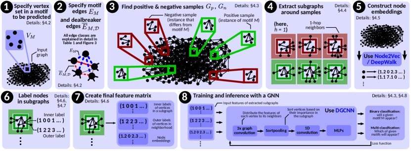
We argue that one could use neural networks to learn a heuristic for motif prediction. Following recent work on link prediction (zhang2018link, ; zhang2020revisiting, ), we use a GNN for this; a GNN may be able to learn link correlations better than a simple hand-designed heuristic. Simultaneously, heuristics are still important as they do not require expensive training. We now describe a GNN architecture called SEAM (learning from Subgraphs, Embeddings and Attributes for Motif prediction). A high-level overview is in § 4.1 and in Figure 4.

4.1. Overview

Let $M=(V_{M},E_{M})$ be a motif to be predicted in $G$. First, we extract the already existing instances of $M$ in $G$, denoted as $G_{p}=(V_{p},E_{p})$; $V_{p}\subseteq V$ and $E_{p}\subseteq E$. We use these instances $G_{p}$ to generate positive samples for training and validation. To generate negative samples (details in § 4.3), we find subgraphs $G_{n}=(V_{n},E_{n})$ that do not form a motif $M$ (i.e., $V_{n}=V_{M}$ and $E_{M}\nsubseteq E_{n}$ or $\overline{E}_{M,\mathcal{D}}\cap E_{n}\neq\emptyset$). Then, for each positive and negative sample, consisting of sets of vertices $V_{p}$ and $V_{n}$, we extract a “subgraph around this sample”, $G_{s}=(V_{s},E_{s})$, with $V_{p}\subseteq V_{s}\subseteq V$ and $E_{p}\subseteq E_{s}\subseteq E$, or $V_{n}\subseteq V_{s}\subseteq V$ and $E_{n}\subseteq E_{s}\subseteq E$ (details in § 4.4). Here, we rely on the insights from SEAL (zhang2018link, ) on their $\gamma$-decaying heuristic, i.e., it is $G_{s}$, the “surroundings” of a given sample (be it positive or negative), that are important in determining whether $M$ appears or not. The nodes of these subgraphs are then appropriately labeled to encode the structural information (details in § 4.6). With these labeled subgraphs, we train our GNN, which classifies each subgraph depending on whether or not vertices $V_{p}$ or $V_{n}$ form the motif $M$. After training, we evaluate the real world accuracy of our GNN by using the validation dataset.

4.2. Specifying Motifs of Interest

The user specifies the motif to be predicted. SEAM provides an interface for selecting (1) vertices $V_{M}$ of interest, (2) motif edges $E_{M}$, and (3) potential deal-breaker edges $\overline{E}_{M,\mathcal{D}}$. The user first picks $V_{M}$ and then they can specify any of up to $2^{\binom{|V_{M}|}{2}}-1$ potential motifs as a target of the prediction. The interface also enables specifying the vertex ordering, or motif’s permutation invariance.

4.3. Positive and Negative Sampling

We need to provide a diverse set of samples to ensure that SEAM works reliably on a wide range of real data. For the positive samples, this is simple because the motif to be predicted ($M$) is specified. Negative samples are more challenging, because – for a given motif – there are many potential “false” motifs. In general, for each motif $M$, we generate negative samples using three strategies. (1) We first select positive samples and then remove a few vertices, replacing them with other nearby vertices (i.e., only a small number of motif edges are missing or only a small number of deal-breaker edges are added). Such negative samples closely resemble the positive ones. (2) We randomly sample $V_{M}$ vertices from the graph; such negative samples are usually sparsely connected and do not resemble the positive ones. (3) We select a random vertex $r$ into an empty set, and then we keep adding randomly selected vertices from the union over the neighborhoods of vertices already in the set, growing a subgraph until reaching the size of $V_{M}$; such negative samples may resemble the positive ones to a certain degree. The final set of negative samples usually contains about 80% samples generated by strategy (1) and 10% each of samples generated by (2) and (3). This distribution could be adjusted based on domain knowledge of the input graph (we also experiment with other ratios). Strategies (2) and (3) are primarily used to avoid overfitting of our model.

As an example, let our motif $M$ be a 3-clique ($|V_{M}|=3$ and $|E_{M}|=3$). Consider a simple approach of generating negative samples, in which one randomly samples 3 vertex indices and verifies if there is a closed 3-clique between them. If we use these samples, in our evaluation for considered real world graphs, this leads to a distribution of 90% unconnected samples $|E_{n}|=0$, 9% samples with $|E_{n}|=1$ and only about 1% of samples with $|E_{n}|=2$. Thus, if we train our GNN with this dataset, it would hardly learn the difference between open 3-cliques $|E_{n}|=2$ and closed 3-cliques $|E_{M}|=3$. Therefore, we provide our negative samples by ensuring that a third of samples are open 3-cliques $|E_{n}|=2$ and another third of samples have one edge $|E_{M}|=1$. For the remaining third of samples, we use the randomly generated vertex indices described above, which are mostly unconnected vertices $|E_{M}|=0$.

For dense subgraphs, the sampling is less straightforward. Overall, the goal is to find samples with edge density being either close to, or far away from, the density threshold of a dense subgraph to be predicted. If the edge density of the sampled subgraph is lower than the density threshold it becomes a negative sample and vice versa. The samples chosen further away from the density threshold are used to prevent overfitting similar to strategies (2) and (3) from above. For this, we grow a set of vertices $R$ (starting with a single random vertex), by iteratively adding selected neighbors of vertices in $R$ such that we approach the desired density.

Overall, we choose equally many positive and negative samples to ensure a balanced dataset. Furthermore, we limit the number of samples if there are too many, by taking a subset of the samples (selected uniformly at random). The positive and negative samples are split into a training dataset and a validation dataset. This split is typically done in a $9/1$ ratio. To ensure an even distribution of all types of samples in these two datasets, we randomly permute the samples before splitting them.

4.4. Extracting Subgraphs Containing Samples

To reduce the computational costs of our GNN, we do not use the entire graph $G$ as input in training or validation. Instead, we rely on recent insights on link prediction with GNNs (zhang2018link, ; zhang2020revisiting, ), which illustrate that it suffices to provide a subgraph capturing the “close surroundings” (i.e., 1–2 hops away) of the vertices we want to predict a link between, cf. Section 2. We take an analogous assumption for motifs (our evaluation confirms the validity of the assumption). For this, we define the “surroundings” of a given motif $M=(V_{M},E_{M})$. For $G=(V,E)$ and $V_{M}\subseteq V$, the $h$-hop enclosing subgraph $G^{h}_{V_{M}}$ is given by the set of nodes $\{i\in V\mid\exists x\in V_{M}:d(i,x)\leq h\}$. To actually extract the subgraph, we simply traverse $G$ starting from vertices in $V_{M}$, for $h$ hops.

4.5. Node Embeddings for More Accuracy

In certain cases, the $h$-hop enclosing subgraph might miss some information about the motif in question (the details of is missed depend on a specific input graph and selected motif). To alleviate this, while simultaneously avoiding sampling a subgraph with large $h$, we also generate a node embedding $X_{E}\in\mathbb{R}^{n\times f}$ which encodes the information about more distant graph regions using random walks. For this, we employ the established node2vec (grover2016node2vec, ) with the parameters from DeepWalk (perozzi2014deepwalk, ). $f$ is the dimension of the low-dimensional vector representation of a node. We generate such a node embedding once and then only append the embedding vectors (corresponding to the nodes in the extracted subgraph) to the feature matrix of each extracted subgraph. We obtain (cf. § 4.6) $X_{s}=\begin{pmatrix}X_{s_{i}}&X_{s_{E}}&X_{H}&X_{L}&X_{E}\end{pmatrix}\in\mathbb{R}^{s\times(d+2f+2k)}.$

Here, we also extend the SEAL approach called negative injection for more effective embeddings (zhang2018link, ; zhang2020revisiting, ). The authors of SEAL observe that if embeddings are constructed using the edge set containing positive training samples, the GNN would focus on fitting this part of information. Thus, SEAL generates embedding based on the edge set containing also negative training samples, which ultimately improves accuracy. In SEAM, we analogously include all potential motif and deal-breaker edges $E^{*}_{M}$ of all training samples to the input graph when generating the node embedding.

4.6. Node Labeling for Structural Features

In order to provide our GNN with as much structural information as possible, we introduce two node labeling schemes. These schemes serve as structural learning features, and we use them when constructing feature matrices of the extracted subgraphs, fed into a GNN. Let $s$ be the total number of vertices in the extracted subgraph $G_{s}$ and $k$ be the number of vertices forming the motif. We call the vertices in the respective samples ($V_{p}$ or $V_{n}$) the inner vertices since they form a motif sample. The rest of the nodes in the subgraph $G_{s}$ are called outer vertices.

The first label is simply an enumeration of all the inner vertices. We call this label the inner label. It enables ordering each vertex according to its role in the motif. For example, to predict a $k$-star, we always assign the inner label 1 to the star central vertex. This inner node label gets translated into a one-hot matrix $H\in\mathbb{N}^{k\times k}$; $H_{ij}=1$ means that the $i$-th vertex in $V_{M}$ receives label $j$. In order to include $H$ into the feature matrix of the subgraph, we concatenate $H$ with a zero matrix $0_{(s-k)k}\in\mathbb{N}^{(s-k)\times k}$, obtaining $X_{H}=(H\quad 0_{(s-k)k})^{T}$.

The second label is called the outer label. The label assigns to each outer vertex its distances to each inner vertex. Thus, each of the $s-k$ outer vertices get $k$ labels. The first of these $k$ labels describes the distance to the vertex with inner label 1. All these outer labels form a labeling matrix $L\in\mathbb{N}^{(s-k)\times k}$, appended with a zero matrix $0_{kk}$, becoming $X_{L}=(0_{kk}\quad L)^{T}\in\mathbb{N}^{s\times k}$. The final feature matrix $X_{s}$ of the respective subgraph $G_{s}$ consists of $X_{H}$, $X_{L}$, the subgraph node embedding matrix $X_{E}$ and the subgraph input feature matrix $X_{s_{i}}\in\mathbb{R}^{s\times d}$; we have $X_{s}=\begin{pmatrix}X_{s_{i}}&X_{E}&X_{H}&X_{L}\end{pmatrix}\in\mathbb{R}^{s\times(d+f+2k)}$; $d$ is the dimension of the input feature vectors and $f$ is the dimension of the node embedding vectors.

4.7. Different Orderings of Motif Vertices

SEAM supports predicting both motifs where vertices have pre-assigned specific roles, i.e., where vertices are permutation dependant, and motifs with vertices that are permutation invariant. The former enables the user to assign vertices meaningful different structural roles (e.g., star roots). The latter enables predicting motifs where the vertex order does not matter. For example, in a clique, the structural roles of all involved vertices are equivalent (i.e., these motifs are vertex-transitive). This is achieved by permuting the inner labels according to the applied vertex permutation.

4.8. Used Graph Neural Network Model

For our GNN model, we use the graph classification neural network DGCNN (zhang2018end, ), used in SEAL (zhang2018link, ; zhang2020revisiting, ). We now summarize its architecture. The first stage of this GNN consist of three graph convolution layers (GConv). Each layer distributes the vertex features of each vertex to its neighbors. Then, we feed the output of each of these GConv layers into a layer called $k$-sortpooling where all vertices are sorted based on their importance in the subgraph. After that, we apply a standard 1D convolution layer followed by a dense layer, followed by a softmax layer to get the prediction probabilities.

The input for our GNN model is the adjacency matrix of the selected $h$-hop enclosing subgraph $G^{h}_{V_{s}}$ together with the feature matrix $X_{s}$. With these inputs, we train our GNN model for 100 epochs. After each epoch, to validate the accuracy, we simply generate $G^{h}_{V_{p}}$ and $G^{h}_{V_{n}}$ as well as their feature matrix $X_{p}$ and $X_{n}$ from our samples in the validation dataset. We know for each set of vertices $V_{p}$ or $V_{n}$, if they form the motif $M$. Thus, we can analyse the accuracy of our model by comparing the predictions with the original information about the motifs. Ultimately, we expect our model to predict the set of vertices $V_{p}$ to form the motif $M$ and the set of vertices $V_{n}$ not to form the motif $M$.

4.9. Computational Complexity of SEAM

We discuss the time complexity of different parts of SEAM, showing that motif prediction in SEAM is computationally feasible even for large graphs and motifs. Assume that $k$, $t$, and $d$ are #vertices in a motif, the number of mined given motifs per vertex, and the maximum degree in a graph, respectively.

First, extracting samples depends on a motif of interest. For example, positive sampling takes $O(nd^{k})$ ($k$-cliques), $O(tm)$ ($k$-stars), $O(nd^{k})$ ($k$-db-stars), and $O(ndk^{3})$ (dense clusters). These complexities assume mining all instances of respective motifs; SEAM further enables fixing the number of samples to find upfront, which further limits the complexities. Negative sampling (of a single instance) takes $O(dk)$ ($k$-cliques), $O(d)$ ($k$-stars), $O(d+k^{2})$ ($k$-db-stars), and $O(ndk^{3})$ (dense clusters). The complexities may be reduced is the user chooses to fix sampling counts. The $h$-hop subgraph extraction, and inner and outer labeling, take – respectively – $O(kd^{2h})$ and $O(k^{2}d^{h})$ time per sample. Finally, finding node embeddings (with Node2Vec) and training as well as inference (with DGCNN) have complexities as described in detail in the associated papers (zhang2018end, ; grover2016node2vec, ); they were illustrated to be feasible even for large datasets.

Figure 5. Comparison of different motif prediction schemes; SEAM is the proposed GNN based architecture. Other baselines use different link prediction schemes as building blocks; CN stands for Common Neighbors, AA stands for Adamic-Adar. We use graphs also used by the SEAL link prediction method (zhang2018link, ; zhang2020revisiting, ). “$k$-db-star” indicate motifs with deal-breaker edges considered. In the presented data, we predict new instances of a given selected motif in a given graph dataset.

5. Evaluation

We now illustrate the advantages of our correlated heuristics and of our learning architecture SEAM. We feature a representative set of results, extended results are in the appendix.

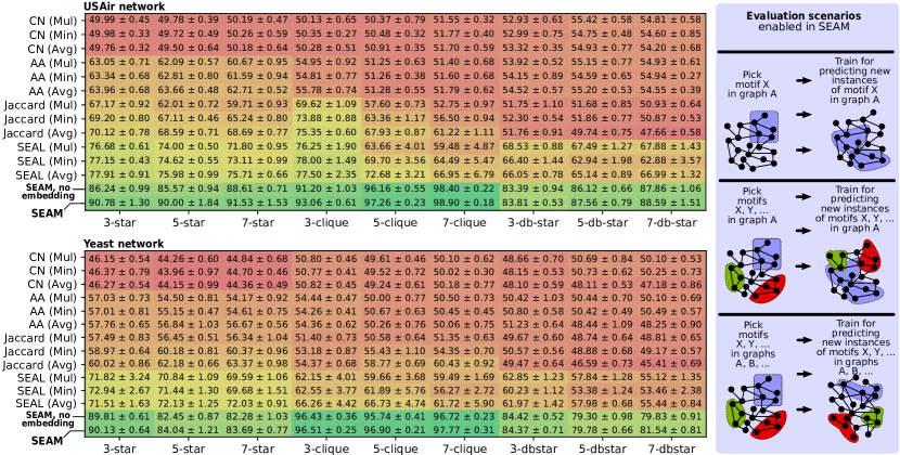
As comparison targets, we use motif prediction based on three link prediction heuristics (Jaccard, Common Neighbors, Adamic-Adar), and on the GNN based state-of-the-art SEAL link prediction scheme (zhang2018link, ; zhang2020revisiting, ). Here, the motif score is derived using a product of link scores with no link correlation (“Mul”). We also consider our correlated heuristics, using link scores, where each score is assigned the same importance (“Avg”, $\mathbf{w}=\mathbf{1}\frac{1}{|E_{M,\mathcal{N}}|}$), or the smallest link score is assigned the highest importance (“Min”). This gives a total of 12 comparison targets. We then consider different variants of SEAM (e.g., with and without embeddings described in § 4.5). More details on the evaluation setting are presented on the right side of Figure 5.

To assess accuracy, we use AUC (Area Under the Curve), a standard metric to evaluate the accuracy of any classification model in machine learning. We also consider a plain fraction of all correct predictions; these results resemble the AUC ones, see the appendix.

Details of parametrization and datasets are included in the appendix. In general, we use the same datasets as in the SEAL paper (zhang2020revisiting, ) for consistent comparisons; these are, among others, Yeast (protein-protein interactions), USAir (airline connections), and Power (a power grid). Overall, our current selection of tested motifs covers the whole motif spectrum in terms of their density: stars (very sparse), communities (moderately sparse and dense, depending on the threshold), and cliques (very dense).

We ensure that the used graphs match our motivation, i.e., they are either evolving or miss higher order structures that are then predicted. For this, we prepare the data so that different edges are removed randomly, imitating noise.

5.1. SEAM GNN vs. SEAL GNN vs.  Heuristics

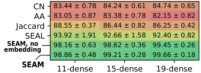
We compare the accuracy of (1) our heuristics from Section 3, (2) a scheme using the SEAL link prediction, and (3) our proposed SEAM GNN architecture. The results for $k$-stars, $k$-cliques, and $k$-db-stars (for networks USAir and Yeast) are in Figure 5 while clusters and communities are analyzed in Figure 6 (“$k$-dense” indicates a cluster of $k$ vertices, with at least 90% of all possible edges present).

Behavior and Advantages of SEAM  First, in Figure 5, we observe that the improvement in accuracy in SEAM almost always scales with the size of the motif. This shows that SEAM captures correlation between different edges (in larger motifs, there is more potential correlation between links). Importantly, the advantages and the capacity of SEAM to capture correlations, also hold in the presence of deal-breaker edges (“$k$-db-star”). Here, we assign links connecting pairs of star outer vertices as deal-breakers (e.g., 7-db-star is a 7-star with 15 deal-breaker edges connecting its arms with one another). We observe that the accuracy for $k$-stars with deal-breaker edges is lower than that for standard $k$-stars. However, SEAM is still the best baseline since it appropriately learns such edges and their impact on the motif appearance. The results in Figure 6 follow similar trends to those in Figure 5; SEAM outperforms all other baselines. Its accuracy also increases with the increasing motif size. Overall, SEAM significantly outperforms both SEAL and heuristics in accuracy, and is the only scheme that captures higher-order characteristics, i.e., its accuracy increases with the amount of link correlations.

Behavior and Advantages of Heuristics  While the core result of our work is the superiority of SEAM in accuracy, our correlated heuristics (“Avg”, “Min”) also to a certain degree improve the motif prediction accuracy over methods that assume link independence (“Mul”). This behavior holds often in a statistically significant way, cf. Jaccard results for 3-cliques, 5-cliques, and 7-cliques. In several cases, the differences are smaller and fall within the standard deviations of respective schemes. Overall, we observe that $AUC_{Mul}<AUC_{Min}<AUC_{Avg}$ (except for $k$-db-stars). This shows that different aggregation schemes have different capacity in capturing the rich correlation structure of motifs. In particular, notice that “Min” is by definition (cf. Proposition 3.1) a lower bound of the score $s(M)$ defined in § 3.5.1. This implies that it is the smallest form of correlation that we can include in our motif score given the convex linear combination function proposed in § 3.5.1.

The main advantage of heuristics over SEAM (or SEAL) is that they do not require training, and are thus overall faster. For example, to predict 100k motif samples, the heuristics take around 2.2 seconds with a standard deviation of 0.05 seconds, while SEAM has a mean execution time (including training) of 1280 seconds with a standard deviation of 30 seconds. Thus, we conclude that heuristics could be preferred over SEAM when training overheads are deemed too high, and/or when the sizes of considered motifs (and thus the amount of link correlations) are small.

Interestingly, the Common Neighbors heuristic performs poorly. This is due to the similar neighborhoods of the edges that have to be predicted. The high similarity of these neighborhoods is caused by our subgraph extraction strategy discussed in Section 4.4, where we select the existing motif edges of the positive samples in such a way as to mimic the edge structure of the negative samples. These results show also that different heuristics do not perform equally with respect to the task of motif prediction and further studies are needed in this direction.

Figure 6. Comparison of prediction schemes as in Figure 5 for predicting dense subgraph motif described in § 4.3. All link prediction based schemes use the same motif score. We use the Yeast graph, also used by the SEAL link prediction method (zhang2018link, ; zhang2020revisiting, ).

The accuracy benefits of SEAM over the best competitor (SEAL using the “Avg” way to compose link prediction scores into motif prediction scores) range from 12% to almost 32%. This difference is even larger for other methods; it is because there comparison targets cannot effectively capture link correlations in motifs. This result shows that the edge correlation in motifs is important to accurately predict a motif’s appearance, and that it benefits greatly from being learned by a neural network.

5.2. Additional Analyses

The only difference in this dataset is the slight drop in accuracy for bigger stars and stars with deal-breaker edges. We conjecture this is because (1) this dataset has many challenging negative samples (4.3) for bigger motifs, and (2) the neighborhoods of negative and positive samples being almost indistinguishable. We also consider a Power graph, see Figure 7. This graph dataset is very sparse with a very low average vertex degree of 2.7 (see the appendix for dataset details). SEAM again offers the best accuracy.

Figure 7. Comparison of different motif prediction schemes for a very sparse Power (power grid) graph. CN: Common Neighbors, AA: Adamic-Adar, Jac: Jaccard, SL: SEAL. “$k$-db-star”: motifs with deal-breaker edges considered.

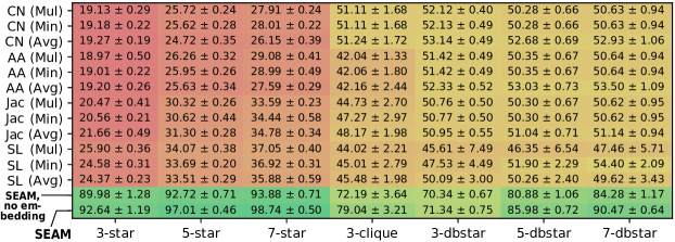
This result clearly shows very low accuracy of SEAL and other motif scores if there are just a few vertices in the neighborhood of the motif. The prediction accuracy for $k$-stars with deal-breaker edges is significantly better. This is caused by the properties of the positive samples discussed in Section 4.3. The prediction task of these positive samples boils down to predicting one motif edge, which has to be added, and several deal-breaker edges, that cannot appear. Due to the sparsity of the motif neighborhood, these deal-breaker edges are often predicted correctly to not appear, which significantly increases the prediction strength of SEAL and all the other motif scores.

We also analyze the impact of additionally using Node2Vec node embeddings (cf. § 4.5). Interestingly, it consistently (by 0.2 – 4%) improves the accuracy while simultaneously reducing the variance in most cases by around 50% for cliques and dense clusters.

We also consider other aspects, for example, we vary the number of existing edges, and even eliminate all such edges; the results follow similar patterns to those observed above.

SEAM’s running times heavily depend on the used model parameters. A full SEAM execution on the Yeast graph dataset with 40,000 training samples and 100 training epochs does typically take between 15–75 minutes (depending on the complexity of the motif, with stars and dense clusters being the fastest and slowest to process, respectively). The used hardware configuration includes an Intel 6130 @2.10GHz with 32 cores and an Nvidia V100 GPU; details are in the appendix.

Other analyses are in the appendix, they include varying the used labeling schemes, training dataset sizes, learning rates, epoch counts, or sizes of enclosing subgraphs.

6. Related Work

Our work is related to various parts of data mining and learning. First, we generalize the established link prediction problem (lu2011link, ; al2006link, ; taskar2004link, ; al2011survey, ; zhang2018link, ; zhang2020revisiting, ; cook2006mining, ; jiang2013survey, ; horvath2004cyclic, ; chakrabarti2006graph, ) into arbitrary higher-order structures, considering inter-link correlations, and providing prediction schemes based on heuristics and GNNs. Next, many works exist on listing, counting, or finding different patterns (also referred to as motifs, graphlets, or subgraphs) (besta2021graphminesuite, ; besta2021sisa, ; chakrabarti2006graph, ; washio2003state, ; lee2010survey, ; rehman2012graph, ; gallagher2006matching, ; ramraj2015frequent, ; jiang2013survey, ; aggarwal2010managing, ; tang2010graph, ; leicht2006vertex, ; besta2017push, ; liben2007link, ; ribeiro2019survey, ; lu2011link, ; al2011survey, ; bron1973algorithm, ; cazals2008note, ; DBLP:conf/isaac/EppsteinLS10, ; DBLP:journals/tcs/TomitaTT06, ; danisch2018listing, ; jabbour2018pushing, ). Our work enables predicting any of such patterns. Moreover, SEAM can use these schemes as subroutines when mining for specific samples. Third, different works analyze the temporal aspects of motifs (kovanen2013temporal, ; torkamani2017survey, ), for example by analyzing the temporal dynamics of editor interactions (jurgens2012temporal, ), temporal dynamics of motifs in general time-dependent networks (paranjape2017motifs, ; kovanen2011temporal, ), efficient counting of temporal motifs (liu2019sampling, ), predicting triangles (benson2018simplicial, ; nassar2019pairwise, ), or using motif features for more effective link predictions (abuoda2019link, ). However, none of them considers prediction of general motifs. Moreover, there exists an extensive body of work on graph processing and algorithms, both static and dynamic (also called temporal, time-evolving, or streaming) (besta2019demystifying, ; besta2019practice, ; sakr2020future, ; Besta:2015:AIC:2749246.2749263, ; gianinazzi2018communication, ; besta2020high, ; solomonik2017scaling, ; besta2020substream, ; besta2017slimsell, ; ediger2010massive, ; ediger2012stinger, ; bulucc2011combinatorial, ; kepner2016mathematical, ; mccoll2013new, ; madduri2009faster, ; kepner2016mathematical, ). Still, they do not consider prediction of motifs.

Finally, GNNs have recently become a subject of intense research (wu2020comprehensive, ; zhou2020graph, ; scarselli2008graph, ; zhang2020deep, ; chami2020machine, ; hamilton2017representation, ; bronstein2017geometric, ; kipf2016semi, ; gianinazzi2021learning, ; bronstein2021geometric, ; wu2020comprehensive, ; zhou2020graph, ; zhang2020deep, ; chami2020machine, ; hamilton2017representation, ; bronstein2017geometric, ; zhang2019graph, ). In this work, we use GNNs for making accurate predictions about motif appearance. While we pick DGCNN as a specific model to implement SEAM, other GNN models can also be used; such an analysis is an interesting direction for future work. An interesting venue of future work would be harnessing GNNs for other graph related tasks, such as compression (besta2019slim, ; besta2018survey, ; besta2018log, ). We implement SEAM within the Pytorch Geometric GNN framework. Still, other GNN frameworks could also be used (li2020pytorch, ; fey2019fast, ; zhu2019aligraph, ; wu2021seastar, ; hu2020featgraph, ; zhang2020agl, ). An interesting line of work would be to implement motif prediction using the serverless paradigm (jonas2019cloud, ; mcgrath2017serverless, ; baldini2017serverless, ; copik2020sebs, ), for example within one of recent dedicated serverless engines (thorpe2021dorylus, ).

7. Conclusion & Discussion

Higher-order network analysis is an important approach for mining irregular data. Yet, it lacks methods and tools for predicting the evolution of the associated datasets. For this, we establish a problem of predicting general complex graph structures called motifs, such as cliques or stars. We illustrate its differences to simple link prediction, and then we propose heuristics for motif prediction that are invariant to the motif size and capture potential correlations between links forming a motif. Our analysis enables incorporating domain knowledge, and thus – similarly to link prediction – it can be a foundation for developing motif prediction schemes within specific domains.

While being fast, heuristics leave some space for improvements in prediction accuracy. To address this, we develop a graph neural network (GNN) architecture for predicting motifs. We show that it outperforms the state of the art by up to 32% in area under the curve, offering excellent accuracy, which improves with the growing size and complexity of the predicted motif. We also successfully apply our architecture to predicting more arbitrarily structured clusters, indicating its broader potential in mining irregular data.

Acknowledgements We thank Hussein Harake, Colin McMurtrie, Mark Klein, Angelo Mangili, and the whole CSCS team granting access to the Ault and Daint machines, and for their excellent technical support. We thank Timo Schneider for immense help with computing infrastructure at SPCL. This research received funding from Google European Doctoral Fellowship, Huawei, and the European Research Council (ERC) under the European Union’s Horizon 2020 programme (grant agreement DAPP, No. 678880).

Appendix A: Proofs

We recall the statement of Observation 1 in Section 3.1:

Consider vertices $v_{1},...,v_{k}\in V$. Assuming no edges already connecting $v_{1},...,v_{k}$, there are $2^{\binom{k}{2}}-1$ motifs (with between 1 and $\binom{k}{2}$ edges) that can appear to connect $v_{1},...,v_{k}$.

Proof.

We denote as $E_{k}=\{\{i,j\}:i,j\in V_{k}\land i\neq j\}$ the edge set of the undirected subgraph $(V_{k},E_{k})$ with $V_{k}\subseteq V$. The number of all possible edges between $k$ vertices is $|E_{k}|=\binom{k}{2}$. Any subset of $E_{k}$, with the exception of the empty set, defines a motif. Thus the set of all possible subsets (i.e., the power set $\mathcal{P}$) of $E_{k}$ is the set of motifs. Then, since $|\mathcal{P}(E_{k})|=2^{\binom{k}{2}}$, we subtract the empty set (which we consider as an invalid motif) from the total count to obtain the desired result. ∎

We recall the statement of Proposition 3.1 in Section 3.5:

Let $\{x_{1},...,x_{n}\}$ be any finite collection of elements from $U=\{x\in\mathbb{R}:0\leq x\leq 1\}$. Then, $\forall n\in\mathbb{N}$ we have $\prod_{i=1}^{n}x_{i}\leq\sum_{i=1}^{n}w_{i}x_{i}$, where $w_{i}\geq 0\;\forall i\in\{1,...,n\}$ and subject to the constraint $\sum_{i=1}^{n}w_{i}=1$.

Proof.

We start by noticing that $\prod_{i=1}^{n}x_{i}\leq\min\{x_{1},...,x_{n}\}$. This is trivial to verify if $\exists\;x_{i}=0$ for $i\in\{1,...,n\}$. Otherwise, it can be shown by contradiction: imagine that $\prod_{i=1}^{n}x_{i}>\min\{x_{1},...,x_{n}\}$. We know that $U$ is closed with respect to the product (i.e., $\prod_{i=1}^{n}x_{i}\in U\;\forall\;n\in\mathbb{N}$). Then, we can divide both sides by $\min\{x_{1},...,x_{n}\}$, since we ruled out the division by zero, to obtain $\prod_{i=1}^{n-1}x_{i}>1$. This implies $\prod_{i=1}^{n-1}x_{i}\notin U$, which contradicts that $U$ is closed to the product. For the right side of the original statement, we know by definition that $x_{i}\geq\min\{x_{1},...,x_{n}\}\;\forall i\in\{1,...,n\}$. Since $w_{i}\geq 0$, we can also write that $w_{i}x_{i}\geq w_{i}\min\{x_{1},...,x_{n}\}\;\forall i\in\{1,...,n\}$. Thus, since $U$ is an ordered set, we can state that $\sum_{i=1}^{n}w_{i}x_{i}\geq\sum_{i=1}^{n}w_{i}\min\{x_{1},...,x_{n}\}$. But then, since $\sum_{i=1}^{n}w_{i}\min\{x_{1},...,x_{n}\}=\min\{x_{1},...,x_{n}\}$, we conclude that $\min\{x_{1},...,x_{n}\}\leq\sum_{i=1}^{n}w_{i}x_{i}$. This ends the proof thanks to the transitive property. ∎

We also justify some complexity bounds from § 4.9. Mining $k$-stars is independent of $k$. To find a $k$-star at a given node $x$, one chooses $k-1$ random nodes of $x$. This has a complexity of $O(k+d(x))$. If $k$ is larger than $d(x)$, there is no star and one can skip the node in $O(1)$. Otherwise, it takes $O(d(x))$ to extract a star. Thus, for a given star, we extract $t$ samples in $O(td(x))$. Summing over all nodes is hence $O(tm)$. Next, the bounds for cliques and clusters are straightforward. Finally, for the enclosing subgraph extraction and labeling, we do a BFS starting from each of the $k$ motif vertices that visits all $h$-hop neighbors. Each node has at most $d$ neighbors, hence there is at most $kd^{h}$ nodes in the $h$-hop neighborhood that need to be visited. But, as BFS is also linear in the number of edges, the complexity is $O(kd^{2h}$). The inner labels are a one-hot-encoding of the motif vertices, which can be produced in $O(k^{2}d^{h})$ time. The outer labels are the distances to the motif nodes, which can be computed at the same time as the BFS traversal for the extraction, so it is the overhead of $O(k^{2}d^{h})$.

Appendix B: Details of Datasets

In this section, we provide additional details on the various datasets that we used. We selected networks of different origins (biological, engineering, transportation), with different structural properties (different sparsities and skews in degree distributions).

USAir (batagelj2006pajek, ) is a graph with 332 vertices and 2,126 edges representing US cities and the airline connections between them. The vertex degrees range from 1 to 139 with an average degree of 12.8. Yeast (mering2002comparative, ) is a graph of protein-protein interactions in yeast with 2,375 vertices and 11,693 edges. The vertex degrees range from 1 to 118 with an average of 9.8. Power (watts1998collective, ) is the electrical grid of the Western US with 4,941 vertices and 6,594 edges. The vertex degrees range from 1 to 19 with an average degree of 2.7.

Appendix C: SEAM Model Parameters

We now discuss in more detail the selection of the SEAM model parameters.

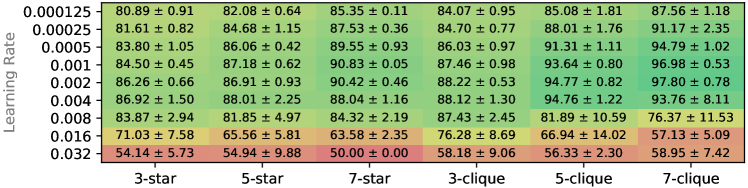
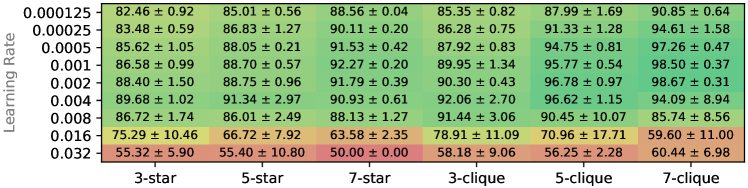
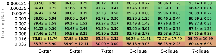
Choosing learning rate and number of epochs

We first describe how we tune the hyperparameters for our motif prediction framework. To find the optimal learning rate for SEAM we try different learning rates as shown in Figures 8, 9 and 10. The associated hyperparameters are highly dependent on the specific motif to be predicted and on the used dataset. As an example, we analyze the hyperparameters for $k$-stars and $k$-cliques on the USAir graph dataset. The plots show that there is a sweet spot for the learning rate at 0.001-0.002. Any value below that rate is too small and our model cannot train its neural network effectively, while for the values above that, the model is unable to learn the often subtle differences between hard negative samples and positive samples. The number of epochs of the learning process can be chosen according to the available computational resources of the user.

Figure 8. AUC-Score comparison for different learning rates on USAir graph. SEAM parameters: proposed labels enabled, proposed embedding disabled. Number of epochs = 50, training dataset size = 100,000.

Figure 9. AUC-Score comparison for different learning rates on USAir graph. SEAM parameters: proposed labels enabled, proposed embedding disabled. Number of epochs = 100, training dataset size = 100,000.

Figure 10. AUC-Score comparison for different learning rates on USAir graph. SEAM parameters: proposed labels enabled, proposed embedding disabled. Number of epochs = 150, training dataset size = 100,000.

Figure 11. AUC-Score comparison for different training dataset sizes on USAir graph. SEAM parameters: proposed labels enabled, proposed embedding enabled. Learning rate = 0.002, number of epochs = 100.

Analysis of different training dataset sizes

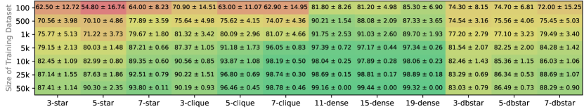
We also analyze the effect of different training dataset sizes on the prediction strength of SEAM. We want to assess the smallest number of samples that still ensures an effective learning process. Figure 11 shows the different accuracy results of SEAM, for different motifs and training dataset sizes. We observe that the accuracy strongly depends on the motif to be predicted. For example, a dense subgraph can be predicted with high accuracy with only 100 training samples. On the other hand, prediction accuracy of the 5-star motif improves proportionally to the amount of training samples while still requiring more samples (than plain dense subgraphs) for a high accuracy score. For all motifs, we set our minimal amount of training samples to 20,000 for positive and for negative ones.

Appendix D: Analysis of Different Variants of Motif Prediction in SEAM

Here, we analyze the effects and contributions from different variants of SEAM. First, we investigate the accuracy improvements due to our proposed labeling scheme in Section 4.6. Then, we empirically justify our approach to only sample the $h$-hop enclosing subgraph for small $h$ (1–2). Finally, we evaluate the performance of every prediction method if there are no motif edges already present.

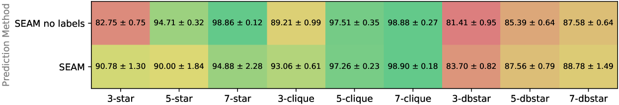
Labeling Scheme vs. Accuracy

Figure 12 shows that our proposed labeling scheme generally has a positive impact on the accuracy of SEAM. The exception is the $k$-star motif. For $k=3$, the labeling scheme significantly improves the accuracy. On the other hand, using $k>3$ reduces the accuracy while simultaneously increasing the variance of test results. This effect can be explained with the implementation details of our labeling scheme. We remove every edges between all the motif vertices to calculate our $k$-dimensional distance labels. This procedure seems to misrepresent the structure of $k$-stars for $k>3$. There are possible improvements to be gained in future work by further optimizing our labeling scheme.

Figure 12. Effect of our proposed labeling scheme on USAir graph. $h$-hop = 1, learning rate = 0.002, number of epochs = 100, training dataset size = 100,000.

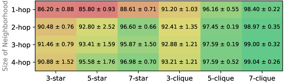
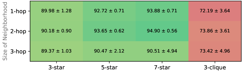
$h$-Hop Enclosing Subgraphs vs. Accuracy

Zhang et al. (zhang2018link, ) motivated the use of small $h$-hop neighborhoods for SEAL with the $\gamma$-decaying heuristic. We now provide additional data to backup this decision in SEAM. Figures 14 and 13 show that in most cases there is not much performance to be gained by sampling an $h$-hop enclosing subgraph with $h>2$. This effect is especially striking for sparse graph datasets like the Power shown in Figure 14. The accuracy starts to drop significantly for $h>2$. The only outlier in our little test was the 5-star motif shown in Figure 13. This effect was most likely caused by the specifics of this particular dataset and it does reflect a trend for other graphs. An additional explanation could also be the non-optimal labeling implementation for the 5-star motif. These special cases do not justify to increase the neighborhood size of the motif in a general case.

Figure 13. Comparison of different $h$-hop enclosing subgraphs used in SEAM, for the USAir graph. Learning rate = 0.002, number of epochs = 100.

Figure 14. Comparison of different $h$-hop enclosing subgraphs used in SEAM, for the Power graph. Learning rate = 0.002, number of epochs = 100, training dataset size = 100,000. The graph does not contain enough 5-cliques and 7-cliques due to its sparsity.

Presence of Motif Edges vs. Accuracy

Figure 15. Comparison of the prediction accuracy of SEAM for different already present motif edges for the Power graph. $h$-hop = 1, learning rate = 0.002, number of epochs = 100, training dataset size = 100,000. The graph does not contain enough 5-cliques and 7-cliques due to its sparsity.

Figure 16. Comparison of the prediction accuracy of SEAM for different already present motif edges for the USAir graph. $h$-hop = 1, learning rate = 0.002, number of epochs = 100, training dataset size = 100,000.

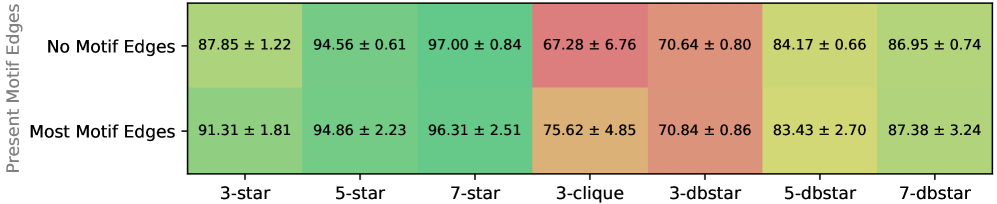
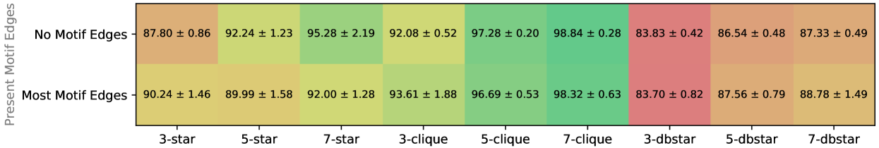
We now illustrate that SEAM also ensures high accuracy when no or very few motif edges are already present, see Figures 15 and 16. Thus, we can conclude that SEAM’s prediction strength relies mostly on the structure of the neighborhood subgraph, embeddings, vertex attributes, and our proposed labeling scheme, and not necessarily on whether a given motif is already partially present. Outliers in this experiment are the 3–clique in the Power graph, the $k$-star motif with $k>3$ in the USAir graph, and the 3-star motif in general. Still, there is no general tendency indicating that SEAM would profit greatly from the presence of most motif edges.

Appendix F: Details of Implementation & Used Hardware

Our implementation of SEAM and SEAL use the PyTorch Geometric Library (fey2019geometric, ). We employ Ray (moritz2017ray, ) for distributed sampling and preprocessing, and RaySGD for distributed training and inference.

To run our experiments, we used the AULT cluster and the Piz Daint cluster at CSCS (CSCS2021, ). For smaller tasks, we used nodes from the AULT cluster such as AULT9/10 (64 AMD EPYC 7501 @ 2GHz processors, 512 GB memory and 4 Nvidia V100 GPUs), AULT23/24 (32 Intel Xeon 6130 @ 2.10GHz processors, 1.5TB memory and 4 Nvidia V100 GPUs), and AULT25 (128 AMD EPYC 7742 @ 2.25GHz processors, 512 GB memory and 4 Nvidia A100 GPUs). For larger, tasks we used our distributed implementation on the Piz Daint cluster (5704 compute nodes, each with 12 Intel Xeon E5-2690 v3 @ 2.60GHz processors, 64 GB memory and a Nvidia Tesla P100 GPU).

References

- [1] G. AbuOda, G. D. F. Morales, and A. Aboulnaga. Link prediction via higher-order motif features. In ECML PKDD, 2019.
- [2] L. A. Adamic and E. Adar. Friends and neighbors on the web. Social networks, 2003.
- [3] C. C. Aggarwal and H. Wang. Managing and mining graph data, volume 40. Springer, 2010.
- [4] M. Al Hasan, V. Chaoji, S. Salem, and M. Zaki. Link prediction using supervised learning. In SDM06: workshop on link analysis, counter-terrorism and security, 2006.
- [5] M. Al Hasan and M. J. Zaki. A survey of link prediction in social networks. In Social network data analytics, pages 243–275. Springer, 2011.
- [6] I. Baldini, P. Castro, K. Chang, P. Cheng, S. Fink, V. Ishakian, N. Mitchell, V. Muthusamy, R. Rabbah, A. Slominski, et al. Serverless computing: Current trends and open problems. In Research Advances in Cloud Computing, pages 1–20. Springer, 2017.
- [7] V. Batagelj and A. Mrvar. Pajek datasets, 2006. http://vlado.fmf.uni-lj.si/pub/networks/data/.
- [8] A. R. Benson et al. Simplicial closure and higher-order link prediction. Proceedings of the National Academy of Sciences, 115(48):E11221–E11230, 2018.
- [9] A. R. Benson, D. F. Gleich, and J. Leskovec. Higher-order organization of complex networks. Science, 353(6295):163–166, 2016.
- [10] M. Besta et al. To push or to pull: On reducing communication and synchronization in graph computations. In HPDC, pages 93–104. ACM, 2017.
- [11] M. Besta et al. Slim graph: Practical lossy graph compression for approximate graph processing, storage, and analytics. In ACM/IEEE Supercomputing, pages 1–25, 2019.
- [12] M. Besta et al. Communication-efficient jaccard similarity for high-performance distributed genome comparisons. In IPDPS, pages 1122–1132. IEEE, 2020.
- [13] M. Besta et al. Graphminesuite: Enabling high-performance and programmable graph mining algorithms with set algebra. arXiv preprint arXiv:2103.03653, 2021.
- [14] M. Besta et al. Sisa: Set-centric instruction set architecture for graph mining on processing-in-memory systems. arXiv preprint arXiv:2104.07582, 2021.
- [15] M. Besta, M. Fischer, T. Ben-Nun, D. Stanojevic, J. D. F. Licht, and T. Hoefler. Substream-centric maximum matchings on fpga. ACM Transactions on Reconfigurable Technology and Systems (TRETS), 13(2):1–33, 2020.
- [16] M. Besta, M. Fischer, V. Kalavri, M. Kapralov, and T. Hoefler. Practice of streaming processing of dynamic graphs: Concepts, models, and systems. arXiv preprint arXiv:1912.12740, 2019.
- [17] M. Besta and T. Hoefler. Accelerating Irregular Computations with Hardware Transactional Memory and Active Messages. In Proc. of the Intl. Symp. on High-Perf. Par. and Dist. Comp., HPDC ’15, pages 161–172, 2015.
- [18] M. Besta and T. Hoefler. Survey and taxonomy of lossless graph compression and space-efficient graph representations. arXiv preprint arXiv:1806.01799, 2018.
- [19] M. Besta, F. Marending, E. Solomonik, and T. Hoefler. Slimsell: A vectorizable graph representation for breadth-first search. In Parallel and Distributed Processing Symposium (IPDPS), 2017 IEEE International, pages 32–41. IEEE, 2017.
- [20] M. Besta and otherd. High-performance parallel graph coloring with strong guarantees on work, depth, and quality. In ACM/IEEE Supercomputing, 2020.
- [21] M. Besta, E. Peter, R. Gerstenberger, M. Fischer, M. Podstawski, C. Barthels, G. Alonso, and T. Hoefler. Demystifying graph databases: Analysis and taxonomy of data organization, system designs, and graph queries. arXiv preprint arXiv:1910.09017, 2019.
- [22] M. Besta, D. Stanojevic, T. Zivic, J. Singh, M. Hoerold, and T. Hoefler. Log (graph): a near-optimal high-performance graph representation. In Proceedings of the 27th International Conference on Parallel Architectures and Compilation Techniques, page 7. ACM, 2018.
- [23] M. Bhattacharyya and S. Bandyopadhyay. Mining the largest quasi-clique in human protein interactome. In EAIS. IEEE, 2009.
- [24] C. Bron and J. Kerbosch. Algorithm 457: finding all cliques of an undirected graph. Communications of the ACM, 16(9):575–577, 1973.
- [25] M. M. Bronstein, J. Bruna, T. Cohen, and P. Veličković. Geometric deep learning: Grids, groups, graphs, geodesics, and gauges. arXiv preprint arXiv:2104.13478, 2021.
- [26] M. M. Bronstein, J. Bruna, Y. LeCun, A. Szlam, and P. Vandergheynst. Geometric deep learning: going beyond euclidean data. IEEE Signal Processing Magazine, 34(4):18–42, 2017.
- [27] A. Buluç and J. R. Gilbert. The combinatorial blas: Design, implementation, and applications. The International Journal of High Performance Computing Applications, 25(4):496–509, 2011.
- [28] W. Cao, Z. Yan, Z. He, and Z. He. A comprehensive survey on geometric deep learning. IEEE Access, 8:35929–35949, 2020.
- [29] F. Cazals and C. Karande. A note on the problem of reporting maximal cliques. Theoretical Computer Science, 407(1-3):564–568, 2008.
- [30] D. Chakrabarti and C. Faloutsos. Graph mining: Laws, generators, and algorithms. ACM computing surveys (CSUR), 38(1):2, 2006.
- [31] I. Chami, S. Abu-El-Haija, B. Perozzi, C. Ré, and K. Murphy. Machine learning on graphs: A model and comprehensive taxonomy. arXiv preprint arXiv:2005.03675, 2020.
- [32] Z. Chen et al. Bridging the gap between spatial and spectral domains: A survey on graph neural networks. arXiv preprint arXiv:2002.11867, 2020.
- [33] D. J. Cook and L. B. Holder. Mining graph data. John Wiley & Sons, 2006.
- [34] M. Copik, G. Kwasniewski, M. Besta, M. Podstawski, and T. Hoefler. Sebs: A serverless benchmark suite for function-as-a-service computing. arXiv preprint arXiv:2012.14132, 2020.
- [35] CSCS. Swiss national supercomputing center, 2021. https://cscs.ch.
- [36] M. Danisch, O. Balalau, and M. Sozio. Listing k-cliques in sparse real-world graphs. In Proceedings of the 2018 World Wide Web Conference on World Wide Web, pages 589–598. International World Wide Web Conferences Steering Committee, 2018.
- [37] D. Ediger et al. Massive streaming data analytics: A case study with clustering coefficients. In IEEE IPDPSW, 2010.
- [38] D. Ediger, R. McColl, J. Riedy, and D. A. Bader. Stinger: High performance data structure for streaming graphs. In 2012 IEEE Conference on High Performance Extreme Computing, pages 1–5. IEEE, 2012.
- [39] D. Eppstein, M. Löffler, and D. Strash. Listing all maximal cliques in sparse graphs in near-optimal time. In Algorithms and Computation - 21st International Symposium, ISAAC 2010, Jeju Island, Korea, December 15-17, 2010, Proceedings, Part I, pages 403–414, 2010.
- [40] M. Fey and J. E. Lenssen. Fast graph representation learning with pytorch geometric. arXiv preprint arXiv:1903.02428, 2019.
- [41] M. Fey and J. E. Lenssen. Fast graph representation learning with pytorch geometric. In Proceedings of the International Conference on Learning Representations, volume 7, 2019.
- [42] B. Gallagher. Matching structure and semantics: A survey on graph-based pattern matching. In AAAI Fall Symposium: Capturing and Using Patterns for Evidence Detection, pages 45–53, 2006.
- [43] L. Gianinazzi et al. Communication-avoiding parallel minimum cuts and connected components. In PPoPP, pages 219–232. ACM, 2018.
- [44] L. Gianinazzi, M. Fries, N. Dryden, T. Ben-Nun, and T. Hoefler. Learning combinatorial node labeling algorithms. arXiv preprint arXiv:2106.03594, 2021.
- [45] D. Gibson, R. Kumar, and A. Tomkins. Discovering large dense subgraphs in massive graphs. In Proceedings of the 31st international conference on Very large data bases, pages 721–732, 2005.
- [46] A. Grover and J. Leskovec. node2vec: Scalable feature learning for networks. In KDD, pages 855–864, 2016.
- [47] W. L. Hamilton et al. Representation learning on graphs: Methods and applications. arXiv preprint arXiv:1709.05584, 2017.
- [48] T. Horváth, T. Gärtner, and S. Wrobel. Cyclic pattern kernels for predictive graph mining. In KDD, pages 158–167. ACM, 2004.
- [49] Y. Hu et al. Featgraph: A flexible and efficient backend for graph neural network systems. arXiv preprint arXiv:2008.11359, 2020.
- [50] S. Jabbour et al. Pushing the envelope in overlapping communities detection. In IDA, pages 151–163. Springer, 2018.
- [51] C. Jiang, F. Coenen, and M. Zito. A survey of frequent subgraph mining algorithms. The Knowledge Engineering Review, 28(1):75–105, 2013.
- [52] E. Jonas, J. Schleier-Smith, V. Sreekanti, C.-C. Tsai, A. Khandelwal, Q. Pu, V. Shankar, J. Carreira, K. Krauth, N. Yadwadkar, et al. Cloud programming simplified: A berkeley view on serverless computing. arXiv preprint arXiv:1902.03383, 2019.
- [53] D. Jurgens and T.-C. Lu. Temporal motifs reveal the dynamics of editor interactions in wikipedia. In AAAI ICWSM, volume 6, 2012.
- [54] L. Katz. A new status index derived from sociometric analysis. Psychometrika, 1953.
- [55] J. Kepner et al. Mathematical foundations of the graphblas. In HPEC, pages 1–9. IEEE, 2016.
- [56] T. N. Kipf and M. Welling. Semi-supervised classification with graph convolutional networks. arXiv preprint arXiv:1609.02907, 2016.
- [57] L. Kovanen et al. Temporal motifs in time-dependent networks. Journal of Statistical Mechanics: Theory and Experiment, 2011(11):P11005, 2011.
- [58] L. Kovanen, M. Karsai, K. Kaski, J. Kertész, and J. Saramäki. Temporal motifs. In Temporal networks, pages 119–133. Springer, 2013.
- [59] V. E. Lee, N. Ruan, R. Jin, and C. Aggarwal. A survey of algorithms for dense subgraph discovery. In Managing and Mining Graph Data, pages 303–336. Springer, 2010.
- [60] E. A. Leicht, P. Holme, and M. E. Newman. Vertex similarity in networks. Physical Review E, 73(2):026120, 2006.
- [61] S. Li et al. Pytorch distributed: Experiences on accelerating data parallel training. arXiv preprint arXiv:2006.15704, 2020.
- [62] X.-L. Li, C.-S. Foo, S.-H. Tan, and S.-K. Ng. Interaction graph mining for protein complexes using local clique merging. Genome Informatics, 2005.
- [63] D. Liben-Nowell and J. Kleinberg. The link-prediction problem for social networks. Journal of the American society for information science and technology, 58(7):1019–1031, 2007.
- [64] P. Liu, A. R. Benson, and M. Charikar. Sampling methods for counting temporal motifs. In ACM WSDM, pages 294–302, 2019.
- [65] L. Lü and T. Zhou. Link prediction in complex networks: A survey. Physica A: statistical mechanics and its applications, 390(6):1150–1170, 2011.
- [66] K. Madduri, D. Ediger, K. Jiang, D. A. Bader, and D. Chavarria-Miranda. A faster parallel algorithm and efficient multithreaded implementations for evaluating betweenness centrality on massive datasets. In Parallel & Distributed Processing, 2009. IPDPS 2009. IEEE International Symposium on, pages 1–8. IEEE, 2009.
- [67] V. Martínez, F. Berzal, and J.-C. Cubero. A survey of link prediction in complex networks. ACM computing surveys (CSUR), 49(4):1–33, 2016.
- [68] R. McColl, O. Green, and D. A. Bader. A new parallel algorithm for connected components in dynamic graphs. In 20th Annual International Conference on High Performance Computing, pages 246–255. IEEE, 2013.
- [69] G. McGrath and P. R. Brenner. Serverless computing: Design, implementation, and performance. In 2017 IEEE 37th International Conference on Distributed Computing Systems Workshops (ICDCSW), pages 405–410. IEEE, 2017.
- [70] P. Moritz et al. Ray: A distributed framework for emerging ai applications. arXiv preprint arXiv:1712.05889, 2017.
- [71] H. Nassar, A. R. Benson, and D. F. Gleich. Pairwise link prediction. In ASONAM, pages 386–393. IEEE, 2019.
- [72] H. Nassar, A. R. Benson, and D. F. Gleich. Neighborhood and pagerank methods for pairwise link prediction. Social Network Analysis and Mining, 10(1):1–13, 2020.
- [73] A. Paranjape, A. R. Benson, and J. Leskovec. Motifs in temporal networks. In Proceedings of the Tenth ACM International Conference on Web Search and Data Mining, pages 601–610, 2017.
- [74] B. Perozzi, R. Al-Rfou, and S. Skiena. Deepwalk: Online learning of social representations. In KDD, pages 701–710, 2014.
- [75] T. Ramraj and R. Prabhakar. Frequent subgraph mining algorithms-a survey. Procedia Computer Science, 47:197–204, 2015.
- [76] S. U. Rehman, A. U. Khan, and S. Fong. Graph mining: A survey of graph mining techniques. In Seventh International Conference on Digital Information Management (ICDIM 2012), pages 88–92. IEEE, 2012.
- [77] P. Ribeiro, P. Paredes, M. E. Silva, D. Aparicio, and F. Silva. A survey on subgraph counting: Concepts, algorithms and applications to network motifs and graphlets. arXiv preprint arXiv:1910.13011, 2019.
- [78] S. Sakr et al. The future is big graphs! a community view on graph processing systems. arXiv preprint arXiv:2012.06171, 2020.
- [79] R. Sato. A survey on the expressive power of graph neural networks. arXiv preprint arXiv:2003.04078, 2020.
- [80] F. Scarselli, M. Gori, A. C. Tsoi, M. Hagenbuchner, and G. Monfardini. The graph neural network model. IEEE transactions on neural networks, 20(1):61–80, 2008.
- [81] E. Solomonik, M. Besta, F. Vella, and T. Hoefler. Scaling betweenness centrality using communication-efficient sparse matrix multiplication. In Proceedings of the International Conference for High Performance Computing, Networking, Storage and Analysis, page 47. ACM, 2017.
- [82] L. Tang and H. Liu. Graph mining applications to social network analysis. In Managing and Mining Graph Data, pages 487–513. Springer, 2010.
- [83] B. Taskar, M.-F. Wong, P. Abbeel, and D. Koller. Link prediction in relational data. In Advances in neural information processing systems, pages 659–666, 2004.
- [84] K. K. Thekumparampil, C. Wang, S. Oh, and L.-J. Li. Attention-based graph neural network for semi-supervised learning. arXiv preprint arXiv:1803.03735, 2018.
- [85] J. Thorpe, Y. Qiao, J. Eyolfson, S. Teng, G. Hu, Z. Jia, J. Wei, K. Vora, R. Netravali, M. Kim, et al. Dorylus: Affordable, scalable, and accurate gnn training over billion-edge graphs. arXiv preprint arXiv:2105.11118, 2021.
- [86] E. Tomita, A. Tanaka, and H. Takahashi. The worst-case time complexity for generating all maximal cliques and computational experiments. Theor. Comput. Sci., 363(1):28–42, 2006.
- [87] S. Torkamani and V. Lohweg. Survey on time series motif discovery. Wiley Interdisciplinary Reviews: Data Mining and Knowledge Discovery, 7(2):e1199, 2017.
- [88] C. Von Mering et al. Comparative assessment of large-scale data sets of protein–protein interactions. Nature, 417(6887):399–403, 2002.
- [89] T. Washio and H. Motoda. State of the art of graph-based data mining. Acm Sigkdd Explorations Newsletter, 5(1):59–68, 2003.
- [90] D. J. Watts and S. H. Strogatz. Collective dynamics of ‘small-world’networks. nature, 393(6684):440–442, 1998.
- [91] S. Wu, F. Sun, W. Zhang, and B. Cui. Graph neural networks in recommender systems: a survey. arXiv preprint arXiv:2011.02260, 2020.
- [92] Y. Wu, K. Ma, Z. Cai, T. Jin, B. Li, C. Zheng, J. Cheng, and F. Yu. Seastar: vertex-centric programming for graph neural networks. In EuroSys, 2021.
- [93] Z. Wu, S. Pan, F. Chen, G. Long, C. Zhang, and S. Y. Philip. A comprehensive survey on graph neural networks. IEEE Transactions on Neural Networks and Learning Systems, 2020.
- [94] C. Zhang, D. Song, C. Huang, A. Swami, and N. V. Chawla. Heterogeneous graph neural network. In KDD, pages 793–803, 2019.
- [95] D. Zhang et al. Agl: a scalable system for industrial-purpose graph machine learning. arXiv preprint arXiv:2003.02454, 2020.
- [96] M. Zhang and Y. Chen. Link prediction based on graph neural networks. arXiv preprint arXiv:1802.09691, 2018.
- [97] M. Zhang, Z. Cui, M. Neumann, and Y. Chen. An end-to-end deep learning architecture for graph classification. In AAAI, volume 32, 2018.
- [98] M. Zhang, P. Li, Y. Xia, K. Wang, and L. Jin. Revisiting graph neural networks for link prediction. arXiv preprint arXiv:2010.16103, 2020.
- [99] S. Zhang, H. Tong, J. Xu, and R. Maciejewski. Graph convolutional networks: a comprehensive review. Computational Social Networks, 6(1):1–23, 2019.
- [100] Z. Zhang, P. Cui, and W. Zhu. Deep learning on graphs: A survey. IEEE Transactions on Knowledge and Data Engineering, 2020.
- [101] J. Zhou, G. Cui, S. Hu, Z. Zhang, C. Yang, Z. Liu, L. Wang, C. Li, and M. Sun. Graph neural networks: A review of methods and applications. AI Open, 1:57–81, 2020.
- [102] R. Zhu, K. Zhao, H. Yang, W. Lin, C. Zhou, B. Ai, Y. Li, and J. Zhou. Aligraph: A comprehensive graph neural network platform. arXiv preprint arXiv:1902.08730, 2019.