Electromagnetic radii of the nucleon in soft-wall holographic QCD

Abstract

We revisit the electromagnetic form factors of the proton and neutron in the original-minimal soft-wall holographic QCD, which has only two parameters, i.e., the mass scale $\kappa$ and the twist parameter of the nucleon $\tau$. We first fix $\tau=3$ by the hard scattering rule, and extract $\kappa=0.402~{}\text{GeV}$ from the world data (including the Mainz A1 data) of the Sachs magnetic form factor of the proton $G_{M}^{p}$. We then predict among others, the charge radius of the proton to be $\bf{r_{p}=0.831\,\pm\,0.008\,\,\text{fm}}$, in perfect agreement with the recent charge radius of the proton measured by the PRad collaboration at Jefferson Lab, and in agreement with the muonic hydrogen experiments. Our prediction for the proton elastic form factor ratio $\mu_{p}G_{E}^{p}/G_{M}^{p}$ is also in very good agreement with the recent high precision Jefferson Lab recoil polarization experiment E08-007 for $Q^{2}=0.3\,-\,0.6~{}\text{GeV}^{2}$, and with the recent high precision Mainz A1 experiment for $Q^{2}<0.13~{}\text{GeV}^{2}$.

I Introduction

The nucleon is a composite hadron with quarks and gluons constituents, the stuff at the origin of all hadronic matter. The quarks are charged and their distribution inside a nucleon is captured by the electric and magnetic charge radii, which measure the charge and current distributions respectively. Precision electron scattering and spectroscopic measurements show a stubborn 4% discrepancy, the so-called proton radius puzzle Carlson (2015); Bernauer (2020); Gao and Vanderhaeghen (2022); Arrington et al. (2021). This is a surprising state of affairs given the fundamental nature of the proton.

The proton structure is the quintessential QCD problem, currently addressed using ab-initio lattice simulations Durr et al. (2008). Empirically, the mass of the proton is known with great accuracy, but its fundamental charge radius is not, as shown in Fig. 1. The high precision elastic e-p scattering measurement of 0.879 fm by Mainz A1 collaboration Bernauer et al. (2010) while consistent with the value of 0.877 fm from the previous hydrogen spectroscopy Fleurbaey et al. (2018), is larger than the reported value of 0.841 fm from muonic hydrogen spectroscopy Antognini et al. (2013), and the values of 0.833 fm and 0.848 fm from the recent hydrogen spectroscopy measurements Bezginov et al. (2019); Grinin et al. (2020). Moreover, the newest e-p measurement by the PRad collaboration at Jefferson Lab has reported a small charge radius of 0.831 fm Xiong et al. (2019). A smaller charge radius is also supported by various re-analysis of the Mainz A1 e-p scattering data Mart and Sulaksono (2013); Lorenz and Meißner (2014); Griffioen et al. (2016); Higinbotham et al. (2016); Horbatsch et al. (2017); Zhou et al. (2019) with few exceptions Lee et al. (2015); Gramolin and Russell (2022). In addition, the recent combined re-analysis of the Mainz A1 and PRad data has also favored a small charge radius Alarcón et al. (2020); Atac et al. (2021a); Lin et al. (2021); Cui et al. (2021); Zhou et al. (2021).

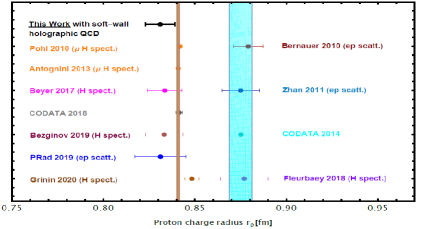
Figure 1: World data for the proton charge radius. The black dot (with its theoretical error bar) is our prediction within the original-minimal soft-wall holographic QCD Karch et al. (2006) with $\tau=3$ and $\kappa=0.402~{}\rm GeV$, see Table 1. The dark-yellow dot is the prediction of Abidin and Carlson Abidin and Carlson (2009) (which is also within the original-minimal soft-wall holographic QCD Karch et al. (2006) with $\tau=3$ and $\kappa=0.350~{}\rm GeV$), see also Table 1. The other dots are the world experimental data for the proton charge radius Pohl 2010 ($\mu$ H spect.) Pohl et al. (2010), Antognini 2013 ($\mu$ H spect.) Antognini et al. (2013), Beyer 2017 (H spect.) Beyer et al. (2017), CODATA 2018 Mohr et al. (2019), Bezignov 2019 (H spect.) Bezginov et al. (2019), PRad 2019 (ep scatt.) Xiong et al. (2019), Grinin 2020 (H spect.) Grinin et al. (2020), Bernauer 2010 (ep scatt.) Bernauer et al. (2010), Zhan 2011 (ep scatt.) Zhan et al. (2011), CODATA 2014 Mohr et al. (2016), and Fleurbaey 2018 (H spect.) Fleurbaey et al. (2018).

All in all, tension seems to exist between e-p scattering measurements of the proton charge radius, and atomic measurements using muonic hydrogen as illustrated in Fig. 1. Although ideas beyond the standard model have been suggested to fix the discrepancy Krasznahorkay et al. (2016); Carlson and Rislow (2012), none so far has been empirically conclusive.

The proton structure emerges from a subtle interplay between the sources composing the nucleon and the primordial glue in the vacuum Zahed (2021). Most of the proton mass arises from the primordial and topological glue at the origin of the spontaneous breaking of chiral symmetry, but its moderatly large size makes it still susceptible to the effects of confinement. This last feature is also shared by the vector mesons, but not the light and more compact pseudoscalar Goldstone bosons. This last observation is further supported by the straight character of the nucleon and rho Regge trajectories, and their remarkable parallelism.

We will address the proton and neutron size problem non-perturbatively in the context of holographic QCD, which among other embodies Regge physics, and provides a field theoretical realization for the dual resonance framework Frampton (1970) postulated decades ago outside the realm of QCD. It is the most economical way of enforcing basic symmetries, including crossing symmetry and unitarity, the key tenets in dispersive analyses. The approach, originates from a conjecture that observables in strongly coupled and conformal gauge theories in the limit of a large number of colors and strong gauge coupling, can be determined from classical fields interacting through gravity, in an anti-de-Sitter space in higher dimensions Maldacena (1998); Aharony et al. (2000). The conjecture has been extended since to non-conformal gauge theories Witten (1998); Karch et al. (2006).

The holographic description of the electromagnetic form factors in the context of the original-minimal soft-wall holographic QCD Karch et al. (2006) was initially addressed in Abidin and Carlson (2009) (with just two parameters, the mass scale $\kappa$ and twist of proton $\tau$) with rather large electromagnetic radii for $\kappa=0.350~{}\text{GeV}$ (fixed by simultaneously fitting the holographic mass of the rho meson and proton to their experimental values, see Table 1), and $\tau=3$ (fixed by the hard scattering rule). Here we show how to overcome this major shortcoming by fixing $\kappa=0.402~{}\text{GeV}$ (fixed by fitting the holographic Sachs magnetic form factor of the proton to the world data (including the Mainz A1 data) of the Sachs magnetic form factor of proton), see Table 1), and Fig. 2. We also fix $\kappa=m_{\rho}/2=0.388~{}\text{GeV}$, and $\tau={m_{N}^{2}}/{m_{\rho}^{2}}+1=2.465$ at low energy, assuming that the nucleon anomalous dimension or the twist $\tau$, runs with the energy scale to asymptote its hard scaling value $\tau=3$ at high energy Lepage and Brodsky (1980), see Table 1. The difference between these two choices of the holographic parameters $\kappa$ and $\tau$, will help us estimate our theoretical uncertainty in determining the electromagnetic radii of the nucleons.

The organization of the paper is as follows: in section II, we write down the holographic Sachs electric and magnetic form factor of the nucleon which are derived in detail, within the original-minimal holographic QCD Karch et al. (2006); Abidin and Carlson (2009). In section III, we show the three possible ways of fixing the only two parameters $\kappa$ and $\tau$ of the original-minimal holographic QCD, and summarize the corresponding predictions for the charge radius of the proton in Table 1. Finally, in section IV, we compute the charge and magnetic radii of both the proton and neutron, and compare the holographic predictions, within the theoretical uncertainties, to the experimental values. We also summarize our results in Table 2. Our conclusions are in V. More details can be found in the Appendices.

II Nucleon electric and magnetic Sachs form factors

We define the standard electric and magnetic Sachs form factors of the proton and neutron as

$$G_{E}^{P,N}(Q) = F_{1}^{P,N}(Q)-\frac{Q^{2}}{4m_{N}^{2}}F_{2}^{P,N}(Q)\,,$$ (II.1)

$$G_{M}^{P,N}(Q) = F_{1}^{P,N}(Q)+F_{2}^{P,N}(Q)\,,$$ (II.2)

where the Dirac $F_{1}(Q)$ and Pauli $F_{2}(Q)$ form factors of proton (P) and neutron (N) in the original-minimal soft-wall holographic QCD Karch et al. (2006) are given by (see the Appendix for their detailed derivation, see also Abidin and Carlson (2009); Vega et al. (2011))

$$F_{1}^{P}(Q) = \left(\frac{a}{2}+\tau\right)\times B(\tau,a+1)+\eta_{P}\times(\tau-1)\times\frac{a(a(\tau-1)-1)}{(a+\tau)(a+\tau+1)}\times B(\tau-1,a+1)\,,$$ (II.3)

$$F_{2}^{P}(Q) = \eta_{P}\times 4(\tau-1)\times\tau\times B(\tau,a+1)\,,$$ (II.4)

$$F_{1}^{N}(Q) = \eta_{N}\times(\tau-1)\times\frac{a(a(\tau-1)-1)}{(a+\tau+1)(a+\tau)}\times B(\tau-1,a+1)\,,$$ (II.5)

$$F_{2}^{N}(Q) = \eta_{N}\times 4(\tau-1)\times\tau\times B(\tau,a+1)\,,$$ (II.6)

Here we have defined $a=Q^{2}/4\kappa^{2}$ with $Q^{2}=-q^{2}\leq 0$, and denoted by $\kappa$ the mass scale, $\tau$ the twist parameter of the nucleon, and by $B(x,y)={\Gamma(x)\Gamma(y)}/{\Gamma(x+y)}$ the Euler beta function. The additional coefficients $\eta_{P,N}=2g_{5}^{2}\times(\eta_{3}\pm\eta_{0})/2$ in (II.3-II.6) follow from the extra couplings $\eta_{0,3}$, for the singlet and triplet contributions of the bulk Pauli contribution Abidin and Carlson (2009).

The Pauli parameter of the proton $\eta_{P}$ can be determined by matching the value of $F_{2}^{P}(0)$ with the experimental data which is $1.793$, i.e.

$$\eta_{P}=\frac{1.793}{C_{3}(0)}=\frac{1.793}{4(\tau-1)}\,.$$ (II.7)

Similarly, the Pauli parameter of the neutron $\eta_{N}$ can be determined by matching the value of $F_{2}^{N}(0)$ with the experimental data which is $-1.913$, i.e.

$$\eta_{N}=\frac{-1.913}{C_{3}(0)}=\frac{-1.913}{4(\tau-1)}\,.$$ (II.8)

Soft-wall AdS/QCD	$\kappa$	$\tau$	$m^{2}_{\rho}=4\kappa^{2}$	$m^{2}_{N}=4\kappa^{2}(\tau-1)$	$\sqrt{\langle r^{p}_{C}\rangle^{2}}$
This Work	0.388 GeV	2.465	$0.775^{2}$ $\text{GeV}^{2}$    (exp.)	$0.938^{2}$ $\text{GeV}^{2}$    (exp.)	0.839   fm (pr.)
This Work	0.402 GeV	3.000	$0.804^{2}$ $\text{GeV}^{2}$    (pr.)	$1.137^{2}$ $\text{GeV}^{2}$    (pr.)	0.831   fm (pr.)
Abidin-Carlson Abidin and Carlson (2009)	0.350 GeV	3.000	$0.700^{2}$ $\text{GeV}^{2}$    (pr.)	$0.990^{2}$ $\text{GeV}^{2}$    (pr.)	0.960   fm (pr.)

Table 1: Comparison of the values of the holographic parameters ($\kappa$ and $\tau$), and the corresponding predictions for the charge radius of the proton $\sqrt{\langle r^{p}_{C}\rangle^{2}}$ in our work (see (IV.14 - IV.15)) within the original-minimal soft-wall holographic QCD Karch et al. (2006), and the work of Abidin and Carlson Abidin and Carlson (2009) (which is also within the original-minimal soft-wall holographic QCD Karch et al. (2006)). Note that pr. and exp. are shorthand for the predicted and experimental values, respectively.

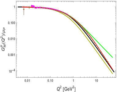
(a)

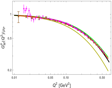
(b)

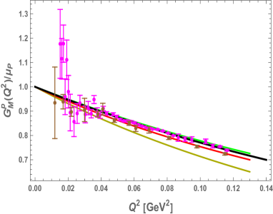
(c)

Figure 2: Sachs magnetic form factor of the proton at high and low momentum transfer. The black-solid curve is our soft-wall holographic QCD result with $\tau=3$ (fixed by the hard counting rule) and $\kappa=0.402\,\text{GeV}$ (extracted from the best fit to the world data (including Mainz A1 data) of Sachs magnetic form factor of proton). The green-solid curve is our soft-wall holographic QCD result with $\tau={m_{N}^{2}}/{m_{\rho}^{2}}+1=2.465$ and $4\kappa^{2}=m_{\rho}^{2}=0.775^{2}\,\text{GeV}^{2}$. The dark-yellow-solid curve is the soft-wall holographic QCD result for $\tau=3$ and $\kappa=0.350~{}\rm GeV$ Abidin and Carlson (2009). The solid-red curve is the Arrington fit to world data (without Mainz A1 data) Arrington et al. (2007) (brown data points). The magenta data points are the Mainz A1 data Bernauer et al. (2014). Throughout, we have used the proton magnetic moment $\mu_{p}=G_{M}^{P}(0)=F_{1}^{P}(0)+F_{2}^{P}(0)=2.793$.

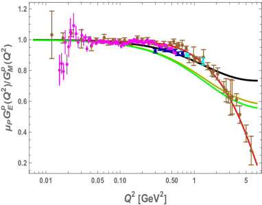
(a)

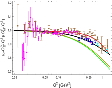
(b)

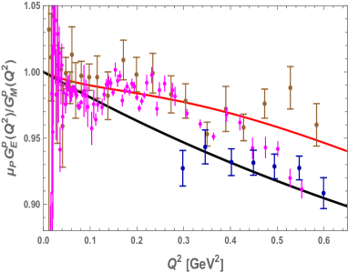
(c)

Figure 3: The ratio of the Sachs electric and magnetic form factor of the proton at high and low momentum transfer. The black-solid curve is our soft-wall holographic QCD result with $\tau=3$ (fixed by the hard counting rule) and $\kappa=0.402\,\text{GeV}$ (extracted from the best fit to the world data (including Mainz A1 data) of Sachs magnetic form factor of proton). The green-solid curve is our soft-wall holographic QCD result with $\tau={m_{N}^{2}}/{m_{\rho}^{2}}+1=2.465$ and $4\kappa^{2}=m_{\rho}^{2}=0.775^{2}\,\text{GeV}^{2}$. The dark-yellow-solid curve is the soft-wall holographic QCD result for $\tau=3$ and $\kappa=0.350~{}\rm GeV$ Abidin and Carlson (2009). The solid-red curve is the Arrington fit Arrington et al. (2007) to the world data (brown data points) (note that the world data (brown data points) is without the Mainz A1 Bernauer et al. (2014) and the recent JLab recoil polarization experimental data Paolone et al. (2010); Zhan et al. (2011)). The magenta data points are the Mainz A1 data Bernauer et al. (2014). The two cyan data points are from the recent high precision JLab recoil polarization experiment E03-104 Paolone et al. (2010). The dark-blue data points are from the recent high precision JLab recoil polarization experiment E08-007 Zhan et al. (2011). Throughout, we have used the proton magnetic moment $\mu_{p}=G_{M}^{P}(0)=F_{1}^{P}(0)+F_{2}^{P}(0)=2.793$.

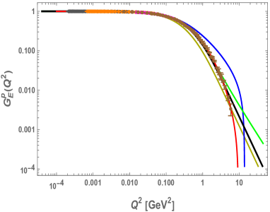
(a)

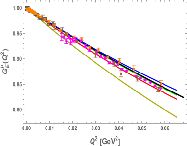
(b)

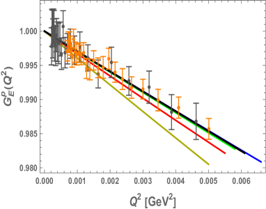
(c)

Figure 4: Sachs electric form factor of the proton at high and low momentum transfer. The black-solid curve is our soft-wall holographic QCD result with $\tau=3$ and $\kappa=0.402\,\text{GeV}$. The green-solid curve is our soft-wall holographic QCD result with $\tau={m_{N}^{2}}/{m_{\rho}^{2}}+1=2.465$ and $4\kappa^{2}=m_{\rho}^{2}=0.775^{2}\,\text{GeV}^{2}$. The dark-yellow-solid curve is the soft-wall holographic QCD result for $\tau=3$ and $\kappa=0.350~{}\rm GeV$ Abidin and Carlson (2009). The solid-blue curve is the PRad fit to PRad data Xiong et al. (2019) (orange and gray data points). The solid-red curve is the Arrington fit to world data (without PRad and Mainz A1 data) Arrington et al. (2007) (brown data points). The magenta data points are the Mainz A1 data Bernauer et al. (2014). Note that in (c) our holographic prediction (solid-black curve) completely overlaps with the PRad fit to PRad data (solid-blue curve).

III Fixing the mass scale $\kappa$ and twist $\tau$, in the original-minimal soft-wall holographic QCD

In this work, we first fix the twist parameter of the proton $\tau=3$, to match the hard counting rule in the large $Q^{2}$ regime (see Appendix C for more details). We then fix the mass scale $\kappa=0.402\,\text{GeV}$ by fitting the holographic Sachs magnetic form factor $G_{M}^{P}(Q)$ (II.2), to the world experimental data (including the Mainz A1 data) on the Sachs magnetic form factor, see Table 1, and the solid-black curves in Fig. 2 - 4.

In this work, we also fix $\kappa$, as was done in the original-minimal soft-wall holographic QCD Karch et al. (2006), by the mass of the $\rho$ meson using the relation $4\kappa^{2}=m_{\rho}^{2}$. Then, we fix $\tau$ by the mass of the nucleon using the relation $m^{2}_{N}=4\kappa^{2}(\tau-1)$. Therefore, for $m_{\rho}=0.775\,\text{GeV}$ and $m_{N}=0.938$, we find $\tau={m_{N}^{2}}/{m_{\rho}^{2}}+1=2.465$ and $\kappa=m_{\rho}/2=0.388\,\text{GeV}$, see Table 1, and the solid-green curves in Fig. 2 - 4.

Our choice is in contrast to the earlier work of Abidin and Carlson Abidin and Carlson (2009), within the original-minimal soft-wall holographic QCD Karch et al. (2006), where they first fixed $\tau=3$ to match the hard counting rule in the large $Q^{2}$ regime, and then fixed $\kappa=0.350\,\text{GeV}$ (by simultaneously fitting to the experimental mass of the rho meson and proton) which gives a smaller $m_{\rho}=2\kappa=0.700\,\text{GeV}$, and a larger mass of the nucleon $m_{N}=2\kappa\sqrt{\tau-1}=0.990\,\text{GeV}$, see Table 1, and the dark-yellow-solid curves in Figs. 2 - 4.

In Fig. 2, we show the magnetic Sachs form factor of the proton. The black-solid curve is our soft-wall holographic QCD result with $\tau=3$ and $\kappa=0.402\,\text{GeV}$. The green-solid curve is our soft-wall holographic QCD result with $\tau={m_{N}^{2}}/{m_{\rho}^{2}}+1=2.465$ and $4\kappa^{2}=m_{\rho}^{2}=0.775^{2}\,\text{GeV}^{2}$. The dark-yellow-solid curve is the soft-wall holographic QCD result for $\tau=3$ and $\kappa=0.350~{}\rm GeV$ Abidin and Carlson (2009). The solid-red curve is the Arrington fit to world data (without the Mainz A1 data) Arrington et al. (2007) (brown data points). The magenta data points are the Mainz A1 data Bernauer et al. (2014). Throughout, we have used the proton magnetic moment $\mu_{p}=G_{M}^{P}(0)=F_{1}^{P}(0)+F_{2}^{P}(0)=2.793$.

In Fig. 3, we show the ratio of the Sachs electric and magnetic form factor of the proton at high and low momentum transfer. The black-solid curve is our soft-wall holographic QCD result with $\tau=3$ (fixed by the hard counting rule) and $\kappa=0.402\,\text{GeV}$ (extracted from the best fit to the world data (including Mainz A1 data) of Sachs magnetic form factor of proton). The green-solid curve is our soft-wall holographic QCD result with $\tau={m_{N}^{2}}/{m_{\rho}^{2}}+1=2.465$ and $4\kappa^{2}=m_{\rho}^{2}=0.775^{2}\,\text{GeV}^{2}$. The dark-yellow-solid curve is the soft-wall holographic QCD result for $\tau=3$ and $\kappa=0.350~{}\rm GeV$ Abidin and Carlson (2009). The solid-red curve is the Arrington fit Arrington et al. (2007) to the world data (brown data points) (note that the world data (brown data points) is without the Mainz A1 Bernauer et al. (2014) and the recent JLab recoil polarization experimental data Paolone et al. (2010); Zhan et al. (2011)). The magenta data points are the Mainz A1 data Bernauer et al. (2014). The two cyan data points are from the recent high precision JLab recoil polarization experiment E03-104 Paolone et al. (2010). The dark-blue data points are from the recent high precision JLab recoil polarization experiment E08-007 Zhan et al. (2011).

In Fig. 4, we show the electric Sachs form factor of the proton. The black-solid curve is our soft-wall holographic QCD result with $\tau=3$ and $\kappa=0.402\,\text{GeV}$ (fixed using the world data of magnetic Sachs form factor of proton). The green-solid curve is our soft-wall holographic QCD result with $\tau={m_{N}^{2}}/{m_{\rho}^{2}}+1=2.465$ and $4\kappa^{2}=m_{\rho}^{2}=0.775^{2}\,\text{GeV}^{2}$. The dark-yellow-solid curve is the soft-wall holographic QCD result for $\tau=3$ and $\kappa=0.350~{}\rm GeV$ Abidin and Carlson (2009). The solid-blue curve is the PRad fit to PRad data Xiong et al. (2019) (orange and gray data points). The solid-red curve is the Arrington fit to world data (without PRad and Mainz A1 data) Arrington et al. (2007) (brown data points). The magenta data points are the Mainz A1 data Bernauer et al. (2014). Note that our holographic prediction (solid-black curve) completely overlaps with the PRad fit to the PRad data (solid-blue curve) in Fig. 4.c for $Q^{2}<0.006$.

IV Electromagnetic radii

IV.1 Proton

The magnetic radius of the proton is defined as

$$\left<r_{M}^{2}\right>_{p}=-6\bigg{(}\frac{d{\rm ln}G_{M}^{P}(Q)}{dQ^{2}}\bigg{)}_{0}\,\hbar^{2}c^{2}\,,$$ (IV.9)

with $\hbar c=0.197\,\text{GeV}\,\rm fm$. Using (II.2) in (IV.9), we find

$$\left<r_{M}^{2}\right>_{p}=(0.803~{}\rm fm)^{2}$$

$$(\textbf{extracted from world data})\,,$$ (IV.10)

with $\kappa$=0.402 GeV (fixed using the world data (including the Mainz A1 data) of the magnetic Sachs form factor of the proton, see Fig. 2), and $\tau=3$ (fixed by the hard scattering rule). Alternatively, we have

$$\left<r_{M}^{2}\right>_{p}=(0.791~{}\rm fm)^{2}\,,$$ (IV.11)

for $\kappa=m_{\rho}/2=0.388\,\text{GeV}$, and $\tau={m_{N}^{2}}/{m_{\rho}^{2}}+1=2.465$. Combining (IV.1) and (IV.11), we find our final magnetic radius of the proton

$$\left<r_{M}^{2}\right>_{p}=(0.803\pm 0.012~{}\rm fm)^{2}$$

$$(\textbf{extracted from world data})\,,$$ (IV.12)

in good agreement with the average of e-p scattering Mainz A1 data (with the average of the most flexible Spline and Polynomial fits) Bernauer et al. (2014), and world data (with Arrington and Sick (2015) world updated value Arrington and Sick (2015) or equivalently with the extraction of Zhan, et al. (2011) Zhan et al. (2011)), respectively, which is $\left<r_{M}^{2}\right>_{p}^{\frac{1}{2}}=(0.777~{}\rm fm+0.867~{}\rm fm)/2=0.822~{}\rm fm$.

The charge radius of the proton is given by

$$\left<r_{C}^{2}\right>_{p}=-6\bigg{(}\frac{d{\rm ln}G_{E}^{P}(Q)}{dQ^{2}}\bigg{)}_{0}\,\hbar^{2}c^{2}\,.$$ (IV.13)

Using (II.1) in (IV.13), we find

$$\left<r_{C}^{2}\right>_{p}=(0.831~{}\rm fm)^{2}\,,$$ (IV.14)

for $\kappa$=0.402 GeV, and $\tau=3$, see Table 1 - 2. We also find

$$\left<r_{C}^{2}\right>_{p}=(0.839~{}\rm fm)^{2}\,,$$ (IV.15)

for $\kappa$=0.388 GeV, and $\tau=2.465$, see Table 1. Combining (IV.14) and (IV.15), we find our final charge radius of the proton

$$\left<r_{C}^{2}\right>_{p}=(0.831\pm 0.008~{}\rm fm)^{2}~{}(\textbf{prediction})\,,$$

see Fig. 1.

IV.2 Neutron

The magnetic radius of the neutron is defined as

$$\left<r_{M}^{2}\right>_{n}=-6\bigg{(}\frac{d{\rm ln}G_{M}^{N}(Q)}{dQ^{2}}\bigg{)}_{0}\,\hbar^{2}c^{2}\,.$$ (IV.17)

Using (II.2) in (IV.9), we find

$$\left<r_{M}^{2}\right>_{n}=(0.817~{}\rm fm)^{2}\,,$$

with $\kappa$=0.402 GeV, and $\tau=3$. We also find

$$\left<r_{M}^{2}\right>_{n}=(0.810~{}\rm fm)^{2}\,,$$ (IV.19)

for $\kappa=0.388\,\text{GeV}$, and $\tau=2.465$. Combining (IV.2) and (IV.19), we find our final magnetic radius of the neutron

$$\left<r_{M}^{2}\right>_{n}=(0.817\pm 0.007~{}\rm fm)^{2}~{}(\textbf{prediction})\,,$$ (IV.20)

in good agreement with the PDG world average Zyla et al. (2020) $\left<r_{M}^{2}\right>_{n}^{\frac{1}{2}}=0.864~{}\rm fm$.

The charge radius of the neutron is given by

$$\left<r_{C}^{2}\right>_{n}=-6\bigg{(}\frac{dG_{E}^{N}(Q)}{dQ^{2}}\bigg{)}_{0}\,\hbar^{2}c^{2}\,.$$ (IV.21)

Using (II.1) in (IV.21), we find

$$\left<r_{C}^{2}\right>_{n}=(-0.094~{}\rm fm)^{2}\,,$$ (IV.22)

for $\kappa$=0.402 GeV, and $\tau=3$. We also find

$$\left<r_{C}^{2}\right>_{n}=(-0.142~{}\rm fm)^{2}\,,$$ (IV.23)

for $\kappa$=0.388 GeV, and $\tau=2.465$. Combining (IV.22) and (IV.23), we find our final charge radius of the neutron

$$\left<r_{C}^{2}\right>_{n}=(-0.094\pm 0.048~{}\rm fm)^{2}~{}(\textbf{prediction})\,.$$

in good agreement with the average of MAMI, JLab/Hall-A, and CLAS experiments (with H. Atac, et al. (2021) fit Atac et al. (2021b)), and the world data (with Kelly (2004) fit Kelly (2004)), which is $\left<r_{E}^{2}\right>_{n}=(-0.110~{}\rm fm^{2}-0.112~{}\rm fm^{2})/2=-0.111~{}\rm fm^{2}$.

We have summarized our result for the electromagnetic radii of the proton and neutron in Table 2.

Nucleon radii	Experimental values	Soft-wall AdS/QCD [This work]
$\sqrt{\langle r^{p}_{M}\rangle^{2}}$	0.822  fm (e-p world average)	0.803 $\pm$ 0.012  fm (extracted)
$\sqrt{\langle r^{p}_{C}\rangle^{2}}$	0.831 fm (PRad 2019)	0.831 $\pm$ 0.008  fm (predicted)
$\sqrt{\langle r^{p}_{C}\rangle^{2}}$	0.841  fm ($\mu p$ Lamb shift)	0.831 $\pm$ 0.008  fm (predicted)
$\sqrt{\langle r^{n}_{M}\rangle^{2}}$	0.864  fm (PDG world average)	0.817 $\pm$ 0.007  fm (predicted)
$\langle(r^{n}_{C})^{2}\rangle$	-0.111  $\text{fm}^{2}$ (world average)	-0.094 $\pm$ 0.048  $\text{fm}^{2}$ (predicted)

Table 2: Comparison of the soft-wall holographic QCD electromagnetic radii of the proton and neutron with experiment. See text for the references of the quoted experimental values.

V Conclusions

By fixing the twist parameter of the nucleon $\tau=3$, and $\kappa=0.402~{}\text{GeV}$, we have found a much improved description of the world data (including the Mainz A1 Bernauer et al. (2010), Jefferson Lab recoil polarization experiment E08-007 Zhan et al. (2011), and PRad data Xiong et al. (2019)), of both the electric and magnetic Sachs form factors (including their ratio) of the proton. The agreement with the data range from low to high momentum transfers, all within the original-minimal soft-wall holographic QCD Karch et al. (2006); Abidin and Carlson (2009), see Figs. 2 - 4. For example, from our electric Sachs form factor of the proton (II.1), we have found the charge radius of the proton to be $\bf{r_{p}=0.831\,\pm\,0.008\,\,\text{fm}}$ in perfect agreement with the recent charge radius of the proton measured by the PRad collaboration at Jefferson Lab Xiong et al. (2019). Our theoretical error in the charge radius of the proton, stems from our alternative choice of $\tau={m_{N}^{2}}/{m_{\rho}^{2}}+1=2.465$, and $\kappa=m_{\rho}/2=0.388~{}\text{GeV}$, which gives the charge radius of proton to be $r_{p}=0.839\,\,\text{fm}$, see Table 1.

To our knowledge, our holographic framework is the only theoretical work that produces a perfect match to the recent PRad collaboration measurement of the charge radius of the proton. We have also computed the charge and magnetic radii of the neutron, as well as the magnetic radius of the proton, with a good agreement to the experimental values, see Table 2. This is not surprising given the non-perturbative nature of the problem, and the phenomenological success of the original soft-wall holographic QCD construction Karch et al. (2006); Abidin and Carlson (2009); Grigoryan and Radyushkin (2007); Colangelo et al. (2008); Forkel (2008); Vega et al. (2011); Braga and Vega (2012); Mamo and Zahed (2021a, 2020a, b, c), with only three parameters: the mass scale $\kappa$, the twist parameter of the nucleon $\tau$, and the ^′t Hooft coupling constant $\lambda$ (also needed for high energy t-channel diffractive processes).

Holography recovers the old dual description with all its phenomenological successes. As we noted earlier, it is the most economical way of enforcing QCD symmetries, duality and crossing symmetries, all usually sought by dispersive analyses, and yet within a well defined and minimal organisational principle using field theory. The present analyses and results are an illustration of that.

However, holography provides much more. Indeed, the bulk holographic description in higher dimension allows for the assessment of any n-point function on the boundary, using field theoretical methods through dual Witten diagrams, in the double limit of large $N_{c}$ and strong gauge coupling. It is the QCD string made user friendly. It also provides for novel physics for processes at low parton-x Mamo and Zahed (2020a), and for scattering on dense systems as dual to black holes Mamo and Zahed (2020b, c).

Appendix A Soft-wall holographic QCD

A simple way to capture AdS/CFT duality in the non-conformal limit is to model it using a slice of AdS₅ with various bulk fields with assigned anomalous dimensions and pertinent boundary values, in the so-called bottom-up approach which we will follow here using the conventions in our recent work in DIS scattering Mamo and Zahed (2020a, 2021a). We consider AdS₅ with a soft wall with a background metric $g_{MN}=(\eta_{\mu\nu},-1)R^{2}/z^{2}$ with the flat metric $\eta_{\mu\nu}=(1,-1,-1,-1)$ at the boundary. Confinement will be described by a harmonic background dilaton $\phi={\kappa}^{2}z^{2}$.

A.1 Bulk vector mesons

The vector mesons fields $L,R$ are described by the bulk effective action Hirn and Sanz (2005); Domokos et al. (2009); Mamo and Zahed (2021a)

$$S_{M}= -\frac{1}{4g_{5}^{2}}\int d^{5}xe^{-\phi(z)}\sqrt{g}\,g^{MP}g^{NQ}{\rm Tr}\bigg{(}{\cal F}^{L}_{MN}{\cal F}^{L}_{PQ}+{\cal F}^{R}_{MN}{\cal F}^{R}_{PQ}\bigg{)}+\int d^{5}x\,\bigg{(}\omega^{L}_{5}({\cal A})-\omega^{R}_{5}({\cal A})\bigg{)}$$ (A.25)

with the Chern-Simons contribution

$$\omega_{5}({\cal A})=\frac{N_{c}}{24\pi^{2}}\int d^{5}x\,{\rm Tr}\left({\cal AF}^{2}+\frac{1}{2}{\cal A}^{3}{\cal F}-\frac{1}{10}{\cal A}^{5}\right)$$ (A.26)

Here ${\cal F}=d{\cal A}-i{\cal A}^{2}$ and ${\cal A}={\cal A}^{a}T^{a}$ with $T^{0}=\frac{3}{2}{\bf 1_{2}}$ and $T^{i}=\frac{1}{2}\tau^{i}$, with the form notation subsumed. Also the vector fields are given by $V=(R+L)/2$ and the axial-vector fields are given by $A=(R-L)/2$. The coupling $g_{5}$ in (A.25) is fixed by the brane embeddings in bulk, or phenomenologically as ${1}/{g_{5}^{2}}\equiv{N_{c}}/(12\pi^{2})$ Cherman et al. (2009).

The flavor gauge fields solve

$$\Box V^{\mu}+ze^{\kappa^{2}z^{2}}\partial_{z}\Big{(}e^{-\kappa^{2}z^{2}}\frac{1}{z}\partial_{z}V^{\mu}\Big{)}\,=\,0\qquad\Box V_{z}-\partial_{z}\Big{(}\partial_{\mu}V^{\mu}\Big{)}\,=\,0\,.$$ (A.27)

subject to the gauge condition

$$\partial_{\mu}V^{\mu}\,+\,ze^{\kappa^{2}z^{2}}\partial_{z}\Big{(}e^{-\kappa^{2}z^{2}}\frac{1}{z}V_{z}\Big{)}\,=\,0\,,$$ (A.28)

with the boundary condition $V_{\mu}(z,y)|_{z\to 0}\,=\,\epsilon_{\mu}(q)\,e^{-iq\cdot y}$. The non-normalizable solutions are

$$V_{\mu}(z,y) = \epsilon_{\mu}(q)\,e^{-iq\cdot y}\,\Gamma\bigg{(}1-\frac{q^{2}}{4\kappa^{2}}\bigg{)}\,\,\kappa^{2}z^{2}\,\,{\cal U}\bigg{(}1-\frac{q^{2}}{4\kappa^{2}};2;\kappa^{2}z^{2}\bigg{)}$$

$$V_{z}(z,y) = \frac{i}{2}\,\epsilon(q)\cdot q\,e^{-iq\cdot y}\,\,\Gamma\bigg{(}1-\frac{q^{2}}{4\kappa^{2}}\bigg{)}\,\,z\,\,{\cal U}\bigg{(}1-\frac{q^{2}}{4\kappa^{2}};1;\kappa^{2}z^{2}\bigg{)}\,,$$ (A.29)

with $\,{\cal U}(a;b;w)\,$ the confluent hypergeometric functions of the second kind.

The normalizable solutions (vector wavefunctions) are also given by Grigoryan and Radyushkin (2007)

$$\phi_{n}(z)=c_{n}\times\kappa^{2}z^{2}L_{n}^{1}(\kappa^{2}z^{2})\,,$$ (A.30)

with $c_{n}=\sqrt{{2}/{n+1}}$ which is determined from the normalization condition (for the soft-wall model with background dilaton $\phi=\kappa^{2}z^{2}$)

$$\int dz\,\sqrt{g}e^{-\phi}\,(g^{xx})^{2}\,\phi_{n}(z)\phi_{m}(z)=\delta_{nm}\,,$$

Here $L_{n}^{(\alpha)}(\xi)$ are the generalized Laguerre polynomials. Therefore, we have

$$F_{n}=\frac{1}{g_{5}}\bigg{(}-e^{-\phi}\frac{1}{z^{\prime}}\partial_{z^{\prime}}\phi_{n}(z^{\prime})\bigg{)}_{z^{\prime}=\epsilon}=-\frac{2}{g_{5}}c_{n}(n+1)\kappa^{2}\,,$$

with $\phi_{n}(z\rightarrow 0)\approx c_{n}\kappa^{2}z^{2}(n+1)$. Then, defining the decay constant as

$$f_{n}=-{F_{n}}/{m_{n}}\,,$$

we have

$$\phi_{n}(z)=\frac{f_{n}}{m_{n}}\times 2g_{5}\times\kappa^{2}z^{2}L_{n}^{1}(\kappa^{2}z^{2})\,,$$ (A.33)

as required by vector meson dominance (VMD).

We can also write the non-normalizable solution as sum over the normalizable solutions as Grigoryan and Radyushkin (2007)

$$V(q,z)=\sum_{n}\frac{-g_{5}F_{n}\phi_{n}(z)}{q^{2}-m_{n}^{2}}=g_{5}^{2}\times\sum_{n}\frac{f_{n}^{2}}{q^{2}-m_{n}^{2}}\times 2\xi L_{n}^{1}(\xi)\,,$$ (A.34)

with $\xi=\kappa^{2}z^{2}$.

A.2 Bulk Dirac fermions

The bulk Dirac fermion action in a sliced of AdS₅ is

$$S_{F}=\frac{1}{2g_{5}^{2}}\int d^{5}x\,e^{-\phi(z)}\,\sqrt{g}\,\Big{(}\mathcal{L}_{F1}+\mathcal{L}_{F2}\Big{)}+\frac{1}{2g_{5}^{2}}\int d^{4}x\sqrt{-g^{(4)}}\,\Big{(}\mathcal{L}_{UV1}+\mathcal{L}_{UV2}\Big{)}\,,$$

(A.35)

The Dirac and Pauli contributions to ${\cal L}_{F1,2}$ are respectively

$$\mathcal{L}_{\rm Dirac1,2} = \bigg{(}\frac{i}{2}\overline{\Psi}_{1,2}e^{N}_{A}\Gamma^{A}\big{(}\overrightarrow{D}_{N}^{L,R}-\overleftarrow{D}_{N}^{L,R}\big{)}\Psi_{1,2}-(\pm M+V(z))\bar{\Psi}_{1,2}\Psi_{1,2}\bigg{)}\,,$$

$$\mathcal{L}_{\rm Pauli1,2} = \pm 2g_{5}^{2}\times\eta\,\bar{\Psi}_{1,2}e^{M}_{A}e^{N}_{B}\sigma^{AB}{\cal F}^{L,R}_{MN}\Psi_{1,2}\,,$$

with $V(z)={\kappa}^{2}z^{2}$, $e^{N}_{A}=z\delta^{N}_{A}$, $\sigma^{AB}=\frac{i}{2}[\Gamma^{A},\Gamma^{B}]$, and $\omega_{\mu z\nu}=-\omega_{\mu\nu z}=\frac{1}{z}\eta_{\mu\nu}$. The Dirac gamma matrices $\Gamma^{A}=(\gamma^{\mu},-i\gamma^{5})$ are chosen in the chiral representation. They satisfy the flat anti-commutation relation $\{\Gamma^{A},\Gamma^{B}\}=2\eta^{AB}$. The left and right covariant derivatives are defined as

$$\overrightarrow{D}_{N}^{X=L,R}= \overrightarrow{\partial}_{N}+\frac{1}{8}\omega_{NAB}[\Gamma^{A},\Gamma^{B}]-iX_{N}^{a}T^{a}\equiv\overrightarrow{\mathcal{D}}_{N}-iX_{N}^{a}T^{a}$$

$$\overleftarrow{D}_{N}^{X=L,R}= \overleftarrow{\partial}_{N}+\frac{1}{8}\omega_{NAB}[\Gamma^{A},\Gamma^{B}]+iX_{N}^{a}T^{a}\equiv\overleftarrow{\mathcal{D}}_{N}+iX_{N}^{a}T^{a}$$ (A.37)

The nucleon doublet refers to

$$\Psi_{1,2}\equiv\begin{pmatrix}\Psi_{p1,2}\\ \Psi_{n1,2}\end{pmatrix}\,.$$ (A.38)

The nucleon fields in bulk form an iso-doublet $p,n$ with $1,2$ referring to their boundary chirality $1,2=\pm=R,L$ Hong et al. (2007). They are dual to the boundary sources $\Psi_{p1,2}\leftrightarrow{\cal O}_{p,\pm}$ and $\Psi_{n1,2}\leftrightarrow{\cal O}_{n,\pm}$ with anomalous dimensions $\pm M=\pm(\Delta-2)=\pm(\tau-3/2)$.

The equation of motions for the bulk Dirac chiral doublet is

$$\bigg{(}ie^{N}_{A}\Gamma^{A}D_{N}^{L,R}-\frac{i}{2}(\partial_{N}\phi)\,e^{N}_{A}\Gamma^{A}-(\pm M+V(z))\bigg{)}\Psi_{1,2}=0\,,$$ (A.39)

The normalizable solution to (A.39) are

$$\Psi_{1}(p,z) = \psi_{R}(z)\Psi^{0}_{R}(p)+\psi_{L}(z)\Psi^{0}_{L}(p)$$

$$\Psi_{2}(p,z) = \psi_{R}(z)\Psi^{0}_{L}(p)+\psi_{L}(z)\Psi^{0}_{R}(p)$$ (A.40)

with the normalized bulk wave functions

$$\psi_{R}(z)=\tilde{n}_{R}{\xi^{\tau-\frac{3}{2}}}L^{(\tau-2)}_{n}(\xi)=\frac{\tilde{n}_{R}}{\kappa^{\tau-2}}z^{\frac{5}{2}}\xi^{\frac{\tau-2}{2}}L_{n}^{(\tau-2)}(\xi)\,,$$

$$\psi_{L}(z)=\tilde{n}_{L}{\xi^{\tau-1}}L^{(\tau-1)}_{n}(\xi)=\frac{\tilde{n}_{L}}{\kappa^{\tau-1}}z^{\frac{5}{2}}\xi^{\frac{\tau-1}{2}}L_{n}^{(\tau-1)}(\xi)\,,$$

Here $\xi=\kappa^{2}z^{2}$, $L_{n}^{(\alpha)}(\xi)$, $\tilde{n}_{R}=\tilde{n}_{L}\kappa^{-1}\sqrt{\tau-1}$ are the generalized Laguerre, and $\tilde{n}_{L}=\kappa^{\tau}\sqrt{{2}/{\Gamma(\tau)}}$. The free Weyl spinors $\Psi^{0}_{R/L}(p)=P_{\pm}u(p)$ and $\bar{\Psi}^{0}_{R/L}(p)=\bar{u}(p)P_{\mp}$, and the free boundary spinors satisfy

$$\bar{u}(p)u(p)=2m_{N}\qquad\qquad 2m_{N}\times\bar{u}(p^{\prime})\gamma^{\mu}u(p)=\bar{u}(p^{\prime})\left[(p^{\prime}+p)^{\mu}+i\sigma^{\mu\nu}(p^{\prime}-p)_{\nu}\right]u(p)\,.$$ (A.42)

The fermionic spectrum Reggeizes $m_{n}^{2}=4\kappa^{2}(n+\tau-1)$. The assignments $1=+$ and $2=-$ at the boundary are commensurate with the substitutions $\psi_{R,L}\leftrightarrow\mp\psi_{L,R}$ by parity.

Using the Dirac 1-form currents

$$J^{aN}_{L}= \frac{\partial\mathcal{L}_{\rm Dirac1}}{\partial L^{a}_{N}}=\overline{\Psi}_{1}e^{N}_{A}\Gamma^{A}T^{a}\Psi_{1}\,,$$

$$J^{aN}_{R}= \frac{\partial\mathcal{L}_{\rm Dirac2}}{\partial R^{a}_{N}}=\overline{\Psi}_{2}e^{N}_{A}\Gamma^{A}T^{a}\Psi_{2}\,,$$ (A.43)

and Pauli 2-form currents

$$J^{aMN}_{L}= \frac{\partial\mathcal{L}_{\rm Pauli1}}{\partial L^{a}_{MN}}=+2g_{5}^{2}\times\eta^{a}\overline{\Psi}_{1}e^{M}_{A}e^{N}_{B}\sigma^{AB}T^{a}\Psi_{1}\,,$$

$$J^{aMN}_{R}= \frac{\partial\mathcal{L}_{\rm Pauli2}}{\partial R^{a}_{MN}}=-2g_{5}^{2}\times\eta^{a}\overline{\Psi}_{2}e^{M}_{A}e^{N}_{B}\sigma^{AB}T^{a}\Psi_{2}\,.$$ (A.44)

we can rewrite (A.2) with the explicit isoscalar ($a=0$) and isovector ($a=3$) contributions

$$\mathcal{L}_{F1}+\mathcal{L}_{F2}\supset \frac{i}{2}\bar{\Psi}_{1}e^{N}_{A}\Gamma^{A}\big{(}\overrightarrow{\mathcal{D}}_{N}-\overleftarrow{\mathcal{D}}_{N}\big{)}\Psi_{1}-(M+V(z))\bar{\Psi}_{1}\Psi_{1}+\frac{i}{2}\bar{\Psi}_{2}e^{N}_{A}\Gamma^{A}\big{(}\overrightarrow{\mathcal{D}}_{N}-\overleftarrow{\mathcal{D}}_{N}\big{)}\Psi_{2}-(-M+V(z))\bar{\Psi}_{2}\Psi_{2}$$

$$+V_{N}^{0}J_{V}^{0N}+A_{N}^{0}J_{A}^{0N}+V_{N}^{3}J_{V}^{3N}+A_{N}^{3}J_{A}^{3N}+V^{0}_{MN}J_{V}^{0MN}+A^{0}_{MN}J_{A}^{0MN}+V^{3}_{MN}J_{V}^{3MN}+A^{3}_{MN}J_{A}^{3MN}$$

with $J_{V,A}^{aN}=J_{L}^{aN}\pm J_{R}^{aN}$ and $J_{V,A}^{aMN}=J_{L}^{aMN}\mp J_{R}^{aMN}$.

Appendix B Electromagnetic form factors

The electromagnetic form factors for the nucleon in the context of the soft wall model have been originally addressed in Abidin and Carlson (2009), although with a different analysis at low momentum transfer than the one we will present and which will fix the numerical shortcomings they encountered. Holographic QCD maps gauge invariant operators at the boundary with supergravity fields in bulk with pertinent anomalous dimensions. The bulk srting theory is in general difficult to solve, but in the double limit of a large number of colors and strong gauge coupling $\lambda=g^{2}N_{c}$, it reduces to a weakly coupled supergravity in the classical limit in $AdS_{5}$ geometry, with a weak string coupling $g_{string}=g^{2}/4\pi$. The n-point functions at the boundary of $AdS_{5}$ follow from variation of the on-shell supergravity action in bulk with respect to the boundary values. The results are tree-level Feynman graphs with fixed end-points on the boundary also known as Witten diagrams Nastase (2015) (and references therein).

The electromagnetic form factor for the nucleon can be extracted from the normalized boundary-to-bulk Witten diagram for the 3-point function, with pertinent LSZ reduction

$${W}_{V}^{a\mu}(q)=\lim_{p_{2}^{2},p_{1}^{2}\to m_{N}^{2}}{(p_{2}^{2}-m_{N}^{2})(p_{1}^{2}-m_{N}^{2})}\,\frac{\left<{\cal O}_{N}(-p_{2})\,{J}_{V}^{a\mu}(q)\,{\cal O}_{N}(p_{1})\right>}{F_{N}(p_{2})F_{N}(p_{1})}\,,$$ (B.46)

for the isoscalar $a=0$ and the isovector $a=3$ current $J_{V}^{a\mu}$, The nucleon source constant is $F_{N}(p)=\left<0\left|{\cal O}_{N}(0)\right|N(p)\right>$. The electromagnetic current form factors follow from the identification

$$\left<N(p_{2})\left|{J}_{EM}^{\mu}(0)\right|N(p_{1})\right>=\bar{u}(p_{2})\left(F_{1}(Q)\gamma^{\mu}+F_{2}(Q)\frac{i\sigma^{\mu\nu}q_{\nu}}{2m_{n}}\right)u(p_{1})=\frac{1}{3}{W}_{V}^{0\mu}(Q^{2})+{W}_{V}^{3\mu}(Q^{2})={W}_{EM}^{\mu}(Q^{2})$$

with $q^{2}=(p_{2}-p_{1})^{2}=-Q^{2}$ (space-like). Here $N(p)$ refers to the U(2) proton-neutron doublet.

The vector currents ${J}_{V}^{a\mu}$ at the boundary are sourced by the dual bulk vector fields $V_{\mu}^{a}(Q,z\rightarrow 0)$. The Dirac and Pauli contributions to the direct part of the electromagnetic current can be extracted from the pertinent bulk Dirac and Pauli parts of the action in the soft wall model. The Dirac part of the action in (A.2) yields

$$S_{Dirac}^{EM}[i,f]= \frac{1}{2g_{5}^{2}}\,\int dzd^{4}y\sqrt{g}e^{-\phi}\,\frac{z}{R}$$

$$\times\bigg{(}\bar{\Psi}_{1f}\gamma^{N}\Big{(}\frac{1}{3}V_{N}^{0}T^{0}+V_{N}^{3}T^{3}\Big{)}\Psi_{1i}+\bar{\Psi}_{2f}\,\gamma^{N}\Big{(}\frac{1}{3}V_{N}^{0}T^{0}+V_{N}^{3}T^{3}\Big{)}\Psi_{2i}\bigg{)}\,,$$

$$= (2\pi)^{4}\delta^{4}(p^{\prime}-p-q)\times F_{N}(p^{\prime})\times F_{N}(p)$$

$$\times\,\frac{1}{2g_{5}^{2}}\times 2g_{5}^{2}\times e_{N}\times\bar{u}_{s_{f}}(p^{\prime})\not{\epsilon}(q)u_{s_{i}}(p)\times\frac{1}{2}\int\frac{dz}{z^{2M}}\,e^{-\phi}{\mathcal{V}}(Q,z)\,\left({\tilde{\psi}_{L}}^{2}(z)+{\tilde{\psi}_{R}}^{2}(z)\right)\,.$$

Here $M=\tau-\frac{3}{2}$, $\phi=\kappa^{2}z^{2}$, and $\epsilon^{\mu}(q)$ is the polarization of the electromagnetic (EM) probe. In the last equality in (B), we substituted the bulk gauge fields by (A.29), and the bulk fermionic currents in terms of the fermionic fields (A.2). The charge assignments are $e_{N}=1$ for the proton, and $e_{N}=0$ for the neutron. We also use the nucleon (ground state) bulk wave functions given by (A.2)

$$\tilde{\psi}_{R}(z)=n_{R}{\xi^{\tau-\frac{3}{2}}}L^{(\tau-2)}_{0}(\xi)\equiv n_{R}{\xi^{\tau-\frac{3}{2}}}\,,$$

$$\tilde{\psi}_{L}(z)=n_{L}{\xi^{\tau-1}}L^{(\tau-1)}_{0}(\xi)\equiv n_{L}{\xi^{\tau-1}}\,,$$ (B.49)

with the generalized Laguerre polynomials $L_{n}^{(\alpha)}(\xi)$, $\xi=\kappa^{2}z^{2}$, $n_{R}=n_{L}\sqrt{\tau-1}$ and $n_{L}=\kappa^{-(\tau-2)}\sqrt{{2}/{\Gamma(\tau)}}$. We also use the non-normalizable solution to the bulk U(1) gauge field (the bulk-to-boundary vector propagator) (A.29)

$$\mathcal{V}(Q,z) = g_{5}^{2}\times\sum_{n}\frac{-f_{n}^{2}}{Q^{2}+m_{n}^{2}}\times 2\xi L_{n}^{1}(\xi)=\xi\,\Gamma(1+a)\,\,{\cal U}(1+a;2;\xi)=\xi\int_{0}^{1}\frac{dx}{(1-x)^{2}}x^{a}{\rm exp}\Big{(}-\frac{x\,\xi}{1-x}\Big{)}\,,$$

(B.50)

with the decay constant of the vector meson resonances $f_{n}=\frac{\sqrt{2}\kappa}{g_{5}}$, linear Regge trajectory for mass of vector meson resonances $m_{n}^{2}=4\kappa^{2}(n+1)$, $a=Q^{2}/(4\kappa^{2})$, and $\xi=\kappa^{2}z^{2}$. The bulk-to-boundary propagator satisfies ${\cal V}(0,z)={\cal V}(Q,0)=1$.

The Dirac part of the electromagnetic current (B) follows from (B) by variation

$${W}_{EM(Dirac)}^{\mu}(Q^{2})=\bar{u}_{s^{\prime}}(p^{\prime})\gamma^{\mu}u_{s}(p)\times e_{N}\times C_{1}(Q)\equiv\frac{1}{F_{N}(p^{\prime})F_{N}(p)}\frac{\delta S_{Dirac}^{EM}}{\delta\epsilon_{\mu}(q)}$$ (B.51)

or more explicitly

$$C_{1}(Q) = \frac{1}{2}\int\frac{dz}{z^{2M}}\,e^{-\phi}{\mathcal{V}}(Q,z)\,\left({\tilde{\psi}_{L}}^{2}(z)+{\tilde{\psi}_{R}}^{2}(z)\right)=g_{5}^{2}\times\sum_{n}\frac{-1}{Q^{2}+m_{n}^{2}}\times\left[f_{n}^{2}\int\frac{dz}{z^{2M}}\,e^{-\xi}\xi L_{n}^{1}(\xi)\,\left({\tilde{\psi}_{L}}^{2}(z)+{\tilde{\psi}_{R}}^{2}(z)\right)\right]\,,$$

$$= g_{5}^{2}\times\sum_{n}\frac{-1}{Q^{2}+m_{n}^{2}}\times\mathcal{G}_{V_{n}\bar{B}B}=\int_{0}^{1}dx\,\left(\tau\left(1-\frac{x}{2}\right)-\frac{1}{2}\right)\,x^{a}\,(1-x)^{\tau-2}=\frac{(a+2\tau)\Gamma(a+1)\Gamma(\tau)}{2\Gamma(a+\tau+1)}\,,$$

$$= \left(\frac{a}{2}+\tau\right)B(\tau,a+1)\,,$$

where, in the last line, we have defined the Euler beta function $B(x,y)=\frac{\Gamma(x)\Gamma(y)}{\Gamma(x+y)}$. In the second line, we have also defined the vector meson resonances $V_{n}$ coupling to the proton (baryon) $B$ as

$$\mathcal{G}_{V_{n}\bar{B}B}\equiv f_{n}^{2}\int\frac{dz}{z^{2M}}\,e^{-\xi}\xi L_{n}^{1}(\xi)\,\left({\tilde{\psi}_{L}}^{2}(z)+{\tilde{\psi}_{R}}^{2}(z)\right)\,,$$

from which we can conclude that $\mathcal{G}_{V_{n}\bar{B}B}\sim N_{c}$, as expected in the large-$N_{c}$ limit. Note that normalizing $C_{1}(0)=1$ for the proton, fixes $1+\mathcal{O}(N_{c}^{-2})=1$. The form factor readily crosses to time-like (modulo $1/N_{c}$ widths), with all meson-baryon-antibaryon couplings (B) fixed, in the double limit of large $N_{c}$ and strong ^′t Hooft coupling! This clearly shows the relationship with constructions based on dispersive analyses Lin et al. (2021) (and references therein).

The nucleon electromagnetic form factors including the Pauli contribution follows a similar reasoning, with the result for the proton

$$F^{P}_{1}(Q) = C_{1}(Q)+\eta_{P}C_{2}(Q)\,,$$

$$F^{P}_{2}(Q) = \eta_{P}C_{3}(Q)\,,$$ (B.54)

and the neutron

$$F^{N}_{1}(Q) = \eta_{N}C_{2}(Q)\,,$$

$$F^{N}_{2}(Q) = \eta_{N}C_{3}(Q)\,.$$ (B.55)

The additional invariant form factors stem from the Pauli contribution. They are structurally similar to the Dirac one in (B), with

$$C_{2}(Q) = \frac{1}{2}\int\frac{dz}{z^{2M}}\,e^{-\phi}\,z{\partial_{z}\mathcal{V}(Q,z)}\left({\tilde{\psi}_{L}}^{2}(z)-{\tilde{\psi}_{R}}^{2}(z)\right)\,,$$

$$= \int_{0}^{1}dx\,\left(\tau x(\tau x+x-3)+1\right)\,x^{a}\,(1-x)^{\tau-2}\,,$$

$$= \frac{a(a(\tau-1)-1)\Gamma(a+1)\Gamma(\tau)}{\Gamma(a+\tau+2)}\,,$$

$$= (\tau-1)\frac{a(a(\tau-1)-1)}{(a+\tau)(a+\tau+1)}B(\tau-1,a+1)\,,$$

and

$$C_{3}(Q) = 2\int\frac{dz}{z^{2M}}\,e^{-\phi}\,m_{N}z{\mathcal{V}(Q,z)}\tilde{\psi}_{L}(z)\tilde{\psi}_{R}(z)\,,$$

$$= \int_{0}^{1}dx\,\left(4(\tau-1)\tau\right)\,x^{a}(1-x)^{\tau-1}\,,$$

$$= \frac{4(\tau-1)\tau\Gamma(a+1)\Gamma(\tau)}{\Gamma(a+\tau+1)}\,,$$

$$= 4(\tau-1)\tau B(\tau,a+1)\,,$$

with $m_{N}^{2}=4\kappa^{2}(\tau-1)$. Note that the contributions $C_{1,2}(Q)$ to the Dirac form factors are chirality-spin preserving with $LL$ and $RR$ following the $\gamma^{\mu}$ assignment, while the contribution $C_{3}(Q)$ to the Pauli form factor is chirality-spin flipping with $LR$ following the $\sigma^{\mu\nu}$ assignment.

Appendix C Hard scattering rule and the dual resonance model

The hard scaling behavior for the electric form factor Lepage and Brodsky (1980) is recovered at high energy by fixing $\tau\rightarrow 3$. Indeed, the contribution $C_{1}(Q)$ to the Dirac form factor $F_{1}(Q)$ in (B) with $a\gg 1$ and fixed $\tau$, asymptotes

$$C_{1}(Q)=\left(\frac{a}{2}+\tau\right)\times B(\tau,a+1)\approx\frac{1}{2}\frac{\Gamma(\tau)}{a^{\tau-1}}\,,$$ (C.58)

in agreement with the hard scattering rule for $\tau=3$. Similarly, the Pauli contribution $C_{2}(Q)$ to the Dirac form factor $F_{1}(Q)$ in (B), at high momentum with $a\gg 1$ and fixed $\tau$, asymptotes

$$C_{2}(Q) = (\tau-1)\frac{a(a(\tau-1)-1)}{(a+\tau)(a+\tau+1)}B(\tau-1,a+1)\,,$$ (C.59)

$$\approx (\tau-1)\frac{\Gamma(\tau)}{a^{\tau-1}}\,,$$

also in agreement with the hard scattering rule for $\tau=3$. Note that The Pauli term contribution $C_{3}(Q)$ to the Pauli form factor $F_{2}(Q)$ in (B), at high momentum with $a\gg 1$ and fixed $\tau$, asymptotes to

$$C_{3}(Q) = 4\tau(\tau-1)B(\tau,a+1)\approx 4\tau(\tau-1)\frac{\Gamma(\tau)}{a^{\tau}}\,,$$

which is subleading in $1/Q^{2}$.

This scaling law originates from the contribution of the R-spinor (B) in the form factor near the UV boundary, as it dwarfs that of the L-spinor (B) when inserted in the integral (B), with the bulk-to-boundary propagator ${\cal V}(Q,z\sim 1/Q)\approx 1$. More specifically, the integrand in (B) gives

$$\bigg{(}\frac{z}{z^{2M}}\bigg{)}\times\xi^{2\tau-3}(1+\xi)\approx\frac{z^{4\tau-6}}{z^{2\tau-4}}\approx\bigg{(}\frac{1}{Q^{2}}\bigg{)}^{\tau-1}$$ (C.61)

Note that the Pauli contributions in (B) carry integrands with extra $z\sim 1/Q$ suppression near the UV boundary, and are sub leading in $1/Q^{2}$. This is expected since the Pauli term is helicity-flipping.

Finally, we note the close relationship between the nucleon form factor obtained in the old resonance dual model Frampton (1970)

$$\frac{B(r_{V},\frac{1}{2}+a)}{B(r_{V},\frac{1}{2})}$$ (C.62)

and the holographic form factors (C.58-C). In (C.62), the spin rho Regge trajectory is

$$\frac{1}{2}+a=\frac{1}{2}+\alpha^{\prime}t\,,$$

with $r_{V}=\tau-1$ and $\alpha^{\prime}=1/4\kappa^{2}$ the open string or rho meson Regge slope. Since the dual resonance description is rooted in the Veneziano amplitude for open string scattering, it is not surprising that the holographic description which captures the dominant stringy excitations in bulk, yields similar results.

References

• Carlson (2015) C. E. Carlson, Prog. Part. Nucl. Phys. 82, 59 (2015), eprint 1502.05314.
• Bernauer (2020) J. C. Bernauer, EPJ Web Conf. 234, 01001 (2020).
• Gao and Vanderhaeghen (2022) H. Gao and M. Vanderhaeghen, Rev. Mod. Phys. 94, 015002 (2022), eprint 2105.00571.
• Arrington et al. (2021) J. Arrington et al. (2021), eprint 2112.00060.
• Durr et al. (2008) S. Durr et al., Science 322, 1224 (2008), eprint 0906.3599.
• Bernauer et al. (2010) J. C. Bernauer et al. (A1), Phys. Rev. Lett. 105, 242001 (2010), eprint 1007.5076.
• Fleurbaey et al. (2018) H. Fleurbaey, S. Galtier, S. Thomas, M. Bonnaud, L. Julien, F. Biraben, F. Nez, M. Abgrall, and J. Guéna, Phys. Rev. Lett. 120, 183001 (2018), eprint 1801.08816.
• Antognini et al. (2013) A. Antognini et al., Science 339, 417 (2013).
• Bezginov et al. (2019) N. Bezginov, T. Valdez, M. Horbatsch, A. Marsman, A. C. Vutha, and E. A. Hessels, Science 365, 1007 (2019).
• Grinin et al. (2020) A. Grinin et al., Science 370, 1061 (2020).
• Xiong et al. (2019) W. Xiong et al., Nature 575, 147 (2019).
• Mart and Sulaksono (2013) T. Mart and A. Sulaksono, Phys. Rev. C 87, 025807 (2013), eprint 1302.6012.
• Lorenz and Meißner (2014) I. T. Lorenz and U.-G. Meißner, Phys. Lett. B 737, 57 (2014), eprint 1406.2962.
• Griffioen et al. (2016) K. Griffioen, C. Carlson, and S. Maddox, Phys. Rev. C 93, 065207 (2016), eprint 1509.06676.
• Higinbotham et al. (2016) D. W. Higinbotham, A. A. Kabir, V. Lin, D. Meekins, B. Norum, and B. Sawatzky, Phys. Rev. C 93, 055207 (2016), eprint 1510.01293.
• Horbatsch et al. (2017) M. Horbatsch, E. A. Hessels, and A. Pineda, Phys. Rev. C 95, 035203 (2017), eprint 1610.09760.
• Zhou et al. (2019) S. Zhou, P. Giulani, J. Piekarewicz, A. Bhattacharya, and D. Pati, Phys. Rev. C 99, 055202 (2019), eprint 1808.05977.
• Lee et al. (2015) G. Lee, J. R. Arrington, and R. J. Hill, Phys. Rev. D 92, 013013 (2015), eprint 1505.01489.
• Gramolin and Russell (2022) A. V. Gramolin and R. L. Russell, Phys. Rev. D 105, 054004 (2022), eprint 2102.13022.
• Alarcón et al. (2020) J. M. Alarcón, D. W. Higinbotham, and C. Weiss, Phys. Rev. C 102, 035203 (2020), eprint 2002.05167.
• Atac et al. (2021a) H. Atac, M. Constantinou, Z. E. Meziani, M. Paolone, and N. Sparveris, Eur. Phys. J. A 57, 65 (2021a), eprint 2009.04357.
• Lin et al. (2021) Y.-H. Lin, H.-W. Hammer, and U.-G. Meißner, Phys. Lett. B 816, 136254 (2021), eprint 2102.11642.
• Cui et al. (2021) Z.-F. Cui, D. Binosi, C. D. Roberts, and S. M. Schmidt (2021), eprint 2102.01180.
• Zhou et al. (2021) J. Zhou, V. Khachatryan, H. Gao, S. Gorbaty, and D. W. Higinbotham (2021), eprint 2110.02557.
• Karch et al. (2006) A. Karch, E. Katz, D. T. Son, and M. A. Stephanov, Phys. Rev. D 74, 015005 (2006), eprint hep-ph/0602229.
• Abidin and Carlson (2009) Z. Abidin and C. E. Carlson, Phys. Rev. D 79, 115003 (2009), eprint 0903.4818.
• Pohl et al. (2010) R. Pohl et al., Nature 466, 213 (2010).
• Beyer et al. (2017) A. Beyer et al., Science 358, 79 (2017).
• Mohr et al. (2019) P. J. Mohr, D. B. Newell, and B. N. Taylor, CODATA recommended values of the fundamental physical constants: 2018. (2019), URL http://physics.nist.gov/constants.
• Zhan et al. (2011) X. Zhan et al., Phys. Lett. B 705, 59 (2011), eprint 1102.0318.
• Mohr et al. (2016) P. J. Mohr, D. B. Newell, and B. N. Taylor, Journal of Physical and Chemical Reference Data 45, 043102 (2016), URL https://doi.org/10.1063/1.4954402.
• Krasznahorkay et al. (2016) A. J. Krasznahorkay et al., Phys. Rev. Lett. 116, 042501 (2016), eprint 1504.01527.
• Carlson and Rislow (2012) C. E. Carlson and B. C. Rislow, Phys. Rev. D 86, 035013 (2012), eprint 1206.3587.
• Zahed (2021) I. Zahed (2021), eprint 2102.08191.
• Frampton (1970) P. H. Frampton, Phys. Rev. D 1, 3141 (1970).
• Maldacena (1998) J. M. Maldacena, Adv. Theor. Math. Phys. 2, 231 (1998), eprint hep-th/9711200.
• Aharony et al. (2000) O. Aharony, S. S. Gubser, J. M. Maldacena, H. Ooguri, and Y. Oz, Phys. Rept. 323, 183 (2000), eprint hep-th/9905111.
• Witten (1998) E. Witten, Adv. Theor. Math. Phys. 2, 505 (1998), eprint hep-th/9803131.
• Lepage and Brodsky (1980) G. P. Lepage and S. J. Brodsky, Phys. Rev. D 22, 2157 (1980).
• Vega et al. (2011) A. Vega, I. Schmidt, T. Gutsche, and V. E. Lyubovitskij, Phys. Rev. D 83, 036001 (2011), eprint 1010.2815.
• Arrington et al. (2007) J. Arrington, W. Melnitchouk, and J. A. Tjon, Phys. Rev. C 76, 035205 (2007), eprint 0707.1861.
• Bernauer et al. (2014) J. C. Bernauer et al. (A1), Phys. Rev. C 90, 015206 (2014), eprint 1307.6227.
• Paolone et al. (2010) M. Paolone et al., Phys. Rev. Lett. 105, 072001 (2010), eprint 1002.2188.
• Arrington and Sick (2015) J. Arrington and I. Sick, J. Phys. Chem. Ref. Data 44, 031204 (2015), eprint 1505.02680.
• Zyla et al. (2020) P. A. Zyla et al. (Particle Data Group), PTEP 2020, 083C01 (2020).
• Atac et al. (2021b) H. Atac, M. Constantinou, Z. E. Meziani, M. Paolone, and N. Sparveris, Nature Commun. 12, 1759 (2021b), eprint 2103.10840.
• Kelly (2004) J. J. Kelly, Phys. Rev. C 70, 068202 (2004).
• Grigoryan and Radyushkin (2007) H. R. Grigoryan and A. V. Radyushkin, Phys. Rev. D 76, 095007 (2007), eprint 0706.1543.
• Colangelo et al. (2008) P. Colangelo, F. De Fazio, F. Giannuzzi, F. Jugeau, and S. Nicotri, Phys. Rev. D 78, 055009 (2008), eprint 0807.1054.
• Forkel (2008) H. Forkel, Phys. Rev. D 78, 025001 (2008), eprint 0711.1179.
• Braga and Vega (2012) N. R. F. Braga and A. Vega, Eur. Phys. J. C 72, 2236 (2012), eprint 1110.2548.
• Mamo and Zahed (2021a) K. A. Mamo and I. Zahed, Phys. Rev. D 104, 066010 (2021a), eprint 2102.00608.
• Mamo and Zahed (2020a) K. A. Mamo and I. Zahed, Phys. Rev. D 101, 086003 (2020a), eprint 1910.04707.
• Mamo and Zahed (2021b) K. A. Mamo and I. Zahed, Phys. Rev. D 103, 094010 (2021b), eprint 2103.03186.
• Mamo and Zahed (2021c) K. A. Mamo and I. Zahed, Phys. Rev. D 104, 066023 (2021c), eprint 2106.00722.
• Mamo and Zahed (2020b) K. A. Mamo and I. Zahed, Phys. Rev. D 101, 066013 (2020b), eprint 1807.07969.
• Mamo and Zahed (2020c) K. A. Mamo and I. Zahed, Phys. Rev. D 101, 066014 (2020c), eprint 1905.07864.
• Hirn and Sanz (2005) J. Hirn and V. Sanz, JHEP 12, 030 (2005), eprint hep-ph/0507049.
• Domokos et al. (2009) S. K. Domokos, H. R. Grigoryan, and J. A. Harvey, Phys. Rev. D 80, 115018 (2009), eprint 0905.1949.
• Cherman et al. (2009) A. Cherman, T. D. Cohen, and E. S. Werbos, Phys. Rev. C 79, 045203 (2009), eprint 0804.1096.
• Hong et al. (2007) D. K. Hong, T. Inami, and H.-U. Yee, Phys. Lett. B 646, 165 (2007), eprint hep-ph/0609270.
• Nastase (2015) H. Nastase, Introduction to the ADS/CFT Correspondence (Cambridge University Press, 2015), ISBN 978-1-107-08585-5, 978-1-316-35530-5.