The chemistry of chlorine-bearing species in the diffuse interstellar medium, and new SOFIA/GREAT^∗ observations of HCl⁺

Abstract

We have revisited the chemistry of chlorine-bearing species in the diffuse interstellar medium with new observations of the HCl⁺ molecular ion and new astrochemical models. Using the GREAT instrument on board SOFIA, we observed the ${}^{2}\Pi_{3/2}\,J=5/2–3/2$ transition of HCl⁺ near 1444 GHz toward the bright THz continuum source W49N. We detected absorption by diffuse foreground gas unassociated with the background source, and were able to thereby measure the distribution of HCl⁺ along the sight-line. We interpreted the observational data using an updated version of an astrochemical model used previously in a theoretical study of Cl-bearing interstellar molecules. The abundance of HCl⁺ was found to be almost constant relative to the related H₂Cl⁺ ion, but the observed $n({\rm H_{2}Cl^{+}})/n({\rm HCl^{+}})$ abundance ratio exceeds the predictions of our astrochemical model by an order-of-magnitude. This discrepancy suggests that the rate of the primary destruction process for ${\rm H_{2}Cl^{+}}$, dissociative recombination, has been significantly overestimated. For ${\rm HCl^{+}}$, the model predictions can provide a satisfactory fit to the observed column densities along the W49N sight-line while simultaneously accounting for the ${\rm OH^{+}}$ and ${\rm H_{2}O^{+}}$ column densities.

1 Introduction

Hydride molecules, consisting of a single heavy element atom with one or more hydrogen atoms, have been studied extensively in the interstellar medium (ISM). Such molecules are valuable probes of the environment in which they are found; collectively, they provide unique information about the density of cosmic rays, the prevalence of shocks, and the dissipation of interstellar turbulence (Gerin et al. 2016 and references therein). To date, 19 interstellar hydrides have been detected in diffuse interstellar gas clouds containing the elements C, N, O, F, S, Cl, or Ar. For most of these elements, their interstellar hydrides are only a trace constituent in diffuse atomic and molecular clouds; here, the dominant reservoirs are atoms or atomic ions, and hydrides typically account for only $\sim 0.01\%$ the overall gas-phase inventory of a given element (Gerin et al. 2016; their Table 2). The two exceptions are the halogen elements, F and Cl. The very stable hydrogen fluoride molecule typically accounts for $\sim 40\%$ of the gas-phase fluorine in diffuse molecular clouds, and the molecular ions HCl⁺ and H₂Cl⁺ may account for several percent of the gas-phase chlorine.

The great tendency of fluorine and chlorine to form hydride molecules in the diffuse ISM is a consequence of thermochemistry (e.g. Neufeld & Wolfire 2009; hereafter NW09): they are the only two elements that can react exothermically with molecular hydrogen when in their primary ionization state in diffuse atomic clouds (i.e. as F and Cl⁺, respectively). While the observed abundance of HF (e.g. Sonnentrucker et al. 2015) is well accounted for by astrochemical models (NW09), such models have tended to underpredict the observed abundances of H₂Cl⁺ (Lis et al. 2010; Neufeld et al. 2012; 2015) and HCl⁺ (De Luca et al. 2012; hereafter DL12).

In the present paper, we address the puzzle of the interstellar HCl⁺ and H₂Cl⁺ abundances with additional observational and theoretical studies. The only previous detections of interstellar HCl⁺ were obtained by DL12 using the HIFI instrument on the Herschel Space Telescope. DL12 detected the 1444 GHz ${}^{2}\Pi_{3/2}\,J=5/2–3/2$ transition of HCl⁺ in absorption toward the bright THz continuum sources W49N and W31C. The Doppler velocities of the detected absorption indicated that it arose in diffuse foreground gas clouds along the sight-lines to – but physically unassociated with – these background continuum sources. Although these HCl⁺ detections were unequivocal, the extraction of reliable column densities was made more difficult by the complex hyperfine structure of HCl⁺ and by the technical challenges entailed by operating at the required frequency near the very bottom of HIFI Band 6. Several spectra had to be discarded due to insufficient mixer pumping, and instrumental drifts – to which the hot electron bolometer mixers were prone – led to strong standing waves that had to be removed. As a result of these difficulties, the observed HCl⁺ spectra had to be fit by using H₂Cl⁺ as a template for the distribution of HCl⁺ in velocity space along the line-of-sight. This procedure yielded the total HCl⁺ column density along the sight-lines to W49N and W31C but did not permit a determination of the column densities over specific velocity intervals within the absorbing gas. The two sources showed almost identical absorbing column densities of HCl⁺, and very similar HCl⁺ to H₂Cl⁺ abundance ratios.

With the goal of improving the observational data available for the study of interstellar HCl⁺, we have reobserved its ${}^{2}\Pi_{3/2}\,J=5/2–3/2$ ground-state transition toward W49N using the GREAT instrument (Heyminck et al. 2012) on SOFIA . The new observations and data reduction are described in Section 2 below, and the results are discussed in Section 3. We have compared the measured column densities of HCl⁺ and H₂Cl⁺ (the latter observed previously by Neufeld et al. 2015; hereafter N15) with the predictions of a grid of astrochemical models. These predictions are based on the NW09 model, which we have updated to account for several laboratory experiments or theoretical calculations performed in the last decade. These developments required modifications to the adopted rates of several significant processes that form or destroy HCl⁺ and H₂Cl⁺. The astrochemical model is described in Section 4. In Section 5, we discuss the comparison between the astronomical observations and the predictions of the astrochemical model. A brief summary follows in Section 6.

2 New observations and data reduction

The observations of W49N were performed on 2016 May 18 UT with the GREAT receiver on SOFIA. The ${}^{2}\Pi_{3/2}\,J=5/2–3/2$ transition of HCl⁺ was observed in the lower sideband of the L1 receiver. At the observing frequency of 1444 GHz, the half power beam width of the telescope was $\sim 20^{\prime\prime}$. The observations were performed with the AFFTS backend, which provides 16384 spectral channels with a spacing of 244.1 kHz. The dual beam switch mode was used to carry out the observation, with a chopper frequency of 2.5 Hz and the reference positions located 160^′′ on either side of the source along an east-west axis.

Using an independent fit to the dry and the wet content of the atmospheric emission, the raw data were calibrated to the $T_{A}^{*}$ (“forward beam brightness temperature”) scale. The assumed forward efficiency was 0.97 and the uncertainty in the flux calibration is estimated to be $\sim 20\%$ (Heyminck et al. 2012). Additional data reduction was performed using CLASS to rebin the data into 20-channel bins (each corresponding to a velocity width of 1.0$\rm\,km\,s^{-1}$), remove a linear baseline, perform the conversion to a single sideband spectrum, and finally obtain a transmission spectrum by dividing the single sideband antenna temperature, $T_{A}^{*}({\rm SSB})$, by the continuum temperature, $T_{\rm cont}=6.2\,\rm K$. The latter corresponds to a main-beam brightness temperature of 9.1 K, given a main beam efficiency of 0.66 as measured on Jupiter.

3 Results

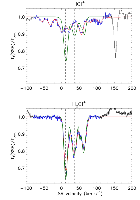
Figure 1: Single-sideband W49N absorption spectra for HCl⁺ (SOFIA/GREAT; top panel; present work) and H₂Cl⁺ (Herschel/HIFI; bottom panel; N15). Histograms: observed spectra normalized relative to the continuum flux. Green curves: hyperfine-deconvolved spectra obtained for the blue portions of the histograms. Red curves: convolution of the green curves with the hyperfine structure. The fitting procedure (see the text for details) optimizes the agreement between the blue portion of the histogram and the red curve.

The HCl⁺ spectrum observed toward W49N is presented in the upper panel of Figure 1 (histogram), where the transmission, $T_{A}^{*}({\rm SSB})/T_{\rm cont}^{*}({\rm SSB})$ is shown as a function of LSR velocity, $v_{\rm LSR}$; the latter is shown for an assumed line rest frequency of 1444.3 GHz. In reality, the effects of lambda-doubling and the nuclear hyperfine interaction split the ${}^{2}\Pi_{3/2}\,J=5/2–3/2$ transition into 18 transitions spanning the 1443.643 – 1444.635 GHz frequency range (DL12, their Table 1). Thus, the observed spectrum (covering only part of this frequency range) represents a convolution between the velocity structure of the absorbing material and the hyperfine structure of the absorption. To deconvolve the observed spectrum and recover the intrinsic velocity structure of the absorbing material, we represented the column density per unit velocity interval as the sum of $N$ Gaussians, each with an adjustable height, width and centroid position. The $3N$ resulting parameters were then varied to optimize the agreement between the observed spectrum and the convolution of the velocity structure with the hyperfine structure. The optimization was performed using the Levenberg-Marquardt algorithm as implemented in the IDL routine mpfit.pro (Markwardt 2009). Five Gaussian components ($N=5$) were found sufficient to provide an excellent fit to the data (red curve in Figure 1). The “hyperfine-convolved” spectrum, shown in green, represents the absorption spectrum that would have resulted in the absence of hyperfine structure.

In the deconvolution procedure described above, only the $[-80,+140]\,{\rm km\,s^{-1}}$ velocity interval was fit (blue portion of the histogram shown in Figure 1). A strong para-NH₂ absorption feature appearing at $+155\,\rm km\,s^{-1}$ was thereby excluded. Gaussian centroid velocities were permitted to range over the $[0,+65]\,{\rm km\,s^{-1}}$ velocity interval for which other molecules are known to absorb along the sight-line to W49N. While the deconvolution procedure should preserve the equivalent width of optically-thin lines, the equivalent width of the deconvolved spectrum significantly exceeds that of the observed spectrum shown in Figure 1. The explanation for this discrepancy is that much of the expected absorption in the convolved spectrum lies outside the frequency range covered by the observations.

For comparison, the histogram in the lower panel of Figure 1 shows H₂Cl⁺ spectrum obtained by Neufeld et al. (2012), together with the deconvolved spectrum (green) and the fit to the observed spectrum (red). The two molecular ions exhibit remarkably similar distributions in $v_{\rm LSR}$, as is demonstrated in Figure 2 (top panel) where the column density per unit velocity interval, $dN/dv$, is shown for each species. Here, we adopted the line frequencies and strengths given by DL12 for HCl⁺ and the Cologne Database for Molecular Spectroscopy (CDMS; Müller et al. 2001, 2005; Endres et al. 2016) for H₂Cl⁺, line frequencies for the latter being based on laboratory spectroscopy reported by Araki et al. (2001). The line strengths are for assumed dipole moments of 1.75 Debye for HCl⁺ (calculation of Cheng et al. 2007) and 1.89 Debye for H₂Cl⁺ (unpublished calculation by H. S. P. Müller 2008).

We have computed the HCl⁺ column density for seven velocity intervals that have been defined in previous studies of W49N (e.g. Indriolo et al. 2015 and references therein). The results are listed in Table 1, along with the column densities of atomic hydrogen (Winkel et al. 2017). We also list the average abundances of HCl⁺ and H₂Cl⁺ (N15) in each velocity interval, relative to atomic hydrogen, along with those of two other molecular ions observed with Herschel (Indriolo et al. 2015): $\rm OH^{+}$ and $\rm H_{2}O^{+}$. Finally, we compute the values of two column density ratios that are expected to probe the molecular hydrogen fraction $N({\rm H_{2}Cl^{+}})/N({\rm HCl^{+}})$ and $N({\rm H_{2}O^{+}})/N({\rm OH^{+}})$. The results for $N({\rm HCl^{+}})/N({\rm H})$ and $N({\rm H_{2}Cl^{+}})/N({\rm H})$ are also represented graphically in Figure 2 (middle panel), as are those for $N({\rm H_{2}Cl^{+}})/N({\rm HCl^{+}})$ (bottom panel).

Table 1: Column densities and column density ratios observed toward W49N

Velocity interval	$N({\rm HCl^{+}})$	$N({\rm H})$	$N({\rm HCl^{+}})/N({\rm H})$	$N({\rm H_{2}Cl^{+}})/N({\rm H})$	$N({\rm H_{2}Cl^{+}})/N({\rm HCl^{+}})$	$N({\rm H_{2}O^{+}})/N({\rm OH^{+}})$
$(\rm km\,s^{-1})$	$(10^{13}\rm\,cm^{-2})$	$(10^{21}\rm\,cm^{-2})$	$\times 10^{9}$	$\times 10^{9}$
$[1,10]$	$1.15\pm 0.34$	$4.44\pm 0.18$	$2.59\pm 0.78$	$2.84\pm 0.85$	$1.10\pm 0.33$	$0.191\pm 0.025$
$[10,17]$	$1.65\pm 0.49$	$3.58\pm 0.13$	$4.61\pm 1.38$	$6.30\pm 1.89$	$1.37\pm 0.41$	$0.347\pm 0.029$
$[17,25]$	$0.68\pm 0.20$	$2.34\pm 0.08$	$2.90\pm 0.87$	$3.43\pm 1.03$	$1.18\pm 0.36$	$0.104\pm 0.011$
$[25,43]$	$1.42\pm 0.43$	$5.58\pm 0.17$	$2.55\pm 0.77$	$5.02\pm 1.51$	$1.97\pm 0.59$	$0.190\pm 0.015$
$[43,51]$	$0.36\pm 0.11$	$1.67\pm 0.05$	$2.13\pm 0.64$	$3.54\pm 1.06$	$1.66\pm 0.50$	$0.134\pm 0.015$
$[51,66]$	$0.97\pm 0.29$	$6.15\pm 0.23$	$1.58\pm 0.47$	$3.46\pm 1.04$	$2.20\pm 0.66$	$0.143\pm 0.014$
$[66,80]$	$0.40\pm 0.12$	$2.89\pm 0.11$	$1.38\pm 0.42$	$2.24\pm 0.67$	$1.62\pm 0.49$	$0.127\pm 0.021$

^a Column densities considered unreliable for this velocity interval, which lies close to the systemic velocity of the background source

The results shown for $N({\rm H_{2}Cl^{+}})$ and $N({\rm HCl^{+}})$, both in Figure 2 and Table 1, are estimates for the total column densities including both stable isotopologs and both spin-isomers for ${\rm H_{2}Cl^{+}}$. Here, we inferred those column densities from the observations of $\rm H^{35}Cl^{+}$ and ortho-${\rm H_{2}^{35}Cl^{+}}$ by assuming and isotopic ratio $\rm{}^{35}Cl/^{37}Cl=3.1$ with no fractionation and an ortho-to-para ratio of 3 for ${\rm H_{2}Cl^{+}}$ (N15).

The overall shape of the HCl⁺ spectrum shown in Figure 1 agrees well with that presented by DL12 (their Figure 1), except in regions where the DL12 results were considered unreliable (shaded regions in their Figure 3) and were excluded from their fit. One notable difference, however, is that all the absorption lines measured in the present study are $\sim 30-40\%$ less deep than those in the DL21 spectrum. This is seen most clearly in the narrow para-$\rm NH_{2}$ feature: in Figure 1 of the present study, the interstellar transmission at line center is 78$\%$, whereas in the DR12 spectrum it is only $\sim 66\%$. Both the DL12 Herschel/HIFI spectrum and the GREAT spectrum obtained with SOFIA were acquired with dual sideband receivers, and we speculate that uncertainties in the sideband gain ratios (SBR) might be cause of these discrepancies. Accordingly, in Table 1, we estimate the uncertainties in the ${\rm HCl^{+}}$ column densities as $\pm 30\%$.

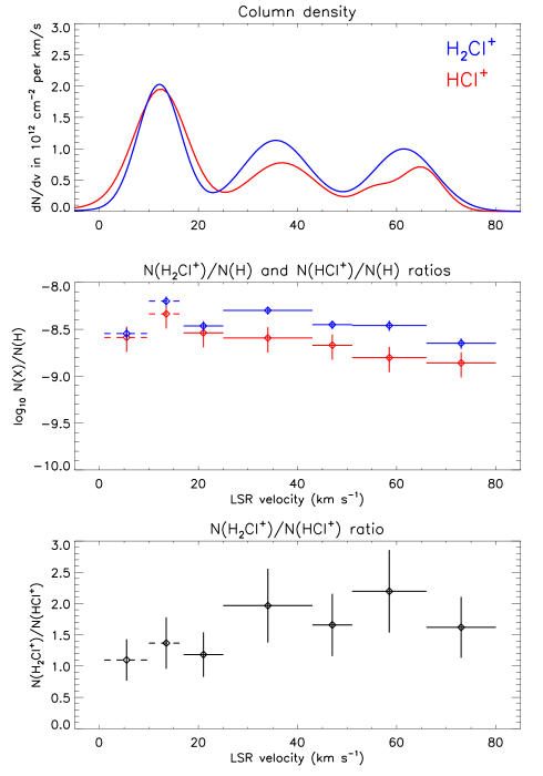
Figure 2: Top panel: column density per unit velocity interval, $dN/dv$, for HCl⁺ (red) and H₂Cl⁺ (blue). Middle panel: average abundances of HCl⁺ (red) and H₂Cl⁺ (blue) relative to atomic hydrogen for 7 velocity intervals defined by Indriolo et al. (2015). Bottom panel: $N({\rm H_{2}Cl^{+}})/N({\rm HCl^{+}})$ for each velocity interval. The data represented by dotted lines in the middle and bottom panels indicate values obtained for material close to the systemic velocity of the background source where the results may be unreliable.

4 Model

To interpret our observations of ${\rm HCl^{+}}$ and ${\rm H_{2}Cl^{+}}$, we have constructed a grid of interstellar cloud models similar to that described by Neufeld & Wolfire (2017; hereafter NW17). In NW17, we obtained predictions for the equilibrium column densities of ${\rm OH^{+}}$ and ${\rm H_{2}O^{+}}$ and other species for a grid of 1440 isochoric cloud models. Our grid covers 9 values of the primary cosmic ray ionization rate per H nucleus, $\zeta_{p}({\rm H})=$ 0.006, 0.02, 0.06, 0.2, 0.6, 2.0, 6.0, 20, and $60\times 10^{-16}\,\rm s^{-1}$; 10 values of the interstellar radiation field, $\chi_{UV}$, defined here as the ratio of the UV energy density to the average interstellar value estimated by Draine (1978): 0.05, 0.1, 0.2, 0.3, 0.5, 1, 2, 3, 5, and 10; and 16 values of the total visual extinction through the cloud, $A_{V}({\rm tot})$: 0.0003, 0.001, 0.003, 0.01, 0.03, 0.1, 0.2, 0.3, 0.5, 0.8, 1.0, 1.5, 2.0, 3.0, 5.0, and 8.0 mag. The grid of models was computed for a single density of H nuclei, $n_{\rm H}=n({\rm H})+2n({\rm H}_{2})=50\,\rm cm^{-3}$. However, the cloud properties can be predicted for other values of $n_{\rm H}$ by means of a simple scaling because the cloud properties are completely determined by $\zeta_{p}({\rm H})/n_{50}$, $\chi_{UV}/n_{50}$, and $A_{V}({\rm tot})$, where $n_{50}\equiv n_{\rm H}/(50\,\rm cm^{-3})$. We will refer to $\zeta_{p}({\rm H})/n_{50}$ and $\chi_{UV}/n_{50}$ as the “environmental parameters,” because they reflect the environment (pressure, cosmic ray density, UV energy density) in which a cloud is located. The third parameter, $A_{V}({\rm tot})$, is related to the cloud column density.

Details of the diffuse cloud model, which solves for the equilibrium physical and chemical structure of a cloud with a slab geometry, have been given in N17, Hollenbach et al. (2012), and references therein: they will not be repeated here except in section 4.2 where minor updates to the model are enumerated. In the present study, our diffuse cloud model was supplemented by the inclusion of additional processes governing the chemistry of chlorine-bearing species, leading to predictions for the column densities of ${\rm HCl^{+}}$ and ${\rm H_{2}Cl^{+}}$.

4.1 Chemical network for chlorine-bearing species

Figure 3 represents the chemical network we adopted, with key reactions shown in red. The basic structure of this network is similar to that discussed by NW09, but several reaction rates have been updated to reflect recent laboratory measurements or new theoretical calculations. The rate coefficients or photorates that we adopted are listed in Table 2.

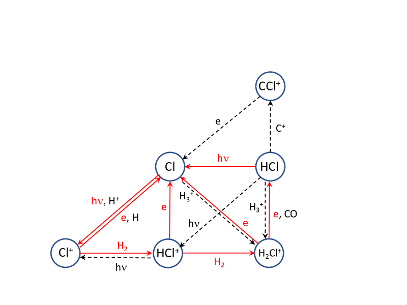
Figure 3: Diagram representing the chemical network for chlorine-bearing species in the ISM. The most important processes in diffuse atomic and molecular clouds are shown with solid red arrows.

Table 2: Reaction list for Cl-bearing species

	Reaction	Rate ($\rm s^{-1})$ or rate coefficient ($\rm cm^{3}\,s^{-1}$)	Referencea
(1)	$\rm Cl+H_{2}\rightarrow HCl+H\phantom{00}$	$2.52\times\rm 10^{-11}\,\exp\,(-2214\,K/{\it T})$ $\phantom{0000000000000}\rm({\it T}\leq 354\,K)$
		$\rm 2.86\times\rm 10^{-12}\,({\it T}/300\,K)^{1.72}\,\exp\,(-1544\,K/{\it T})$ $\,\,\rm({\it T}\geq 354\,K)$
(2)	$\rm HCl+H\rightarrow Cl+H_{2}\phantom{00}$	$1.49\times\rm 10^{-11}\,\exp\,(-1763\,K/{\it T})$ $\phantom{0000000000000}\rm({\it T}\leq 354\,K)$
		$\rm 1.69\times\rm 10^{-12}\,({\it T}/300\,K)^{1.72}\,\exp\,(-1093\,K/{\it T})$ $\,\,\rm({\it T}\geq 354\,K)$
(3)	$\rm C^{+}+HCl\rightarrow CCl^{+}+H$	$1.84\times 10^{-9}\,(T/300\rm\,K)^{-0.202}$
(4)	$\rm H_{3}^{+}+HCl\rightarrow H_{2}+H_{2}Cl^{+}$	$6.35\times 10^{-9}\,(T/300\rm\,K)^{-0.202}$
(5∗)	$\rm Cl^{+}+H_{2}\rightarrow HCl^{+}+H$	$1.0\times\rm 10^{-9}$
(6∗)	$\rm HCl^{+}+H_{2}\rightarrow H_{2}Cl^{+}+H$	$1.3\times\rm 10^{-9}$
(7)	$\rm CCl^{+}+e\rightarrow C+Cl$	$2.0\times 10^{-7}\,(T/300\rm\,K)^{-0.5}$
(8∗)	$\rm HCl^{+}+e\rightarrow H+Cl$	Fitting formula given by N13	N13
(9∗)	$\rm H_{2}Cl^{+}+e\rightarrow products$	$4.3\times 10^{-7}\,(T/300\rm\,K)^{-0.5}$	N18
(10)	$\rm H_{2}Cl^{+}+CO\rightarrow HCl+HCO^{+}$	$\rm 7.8\times 10^{-10}\,$
(11)	$\rm H_{2}Cl^{+}+H_{2}O\rightarrow HCl+H_{3}O^{+}$	$3.7\times 10^{-9}\,(T/300\rm\,K)^{-0.194}$
(12)	$\rm Cl+H_{3}^{+}\rightarrow H_{2}Cl^{+}+H$	$1.0\times\rm 10^{-9}$
(13)	$\rm HCl+h\nu\rightarrow H+Cl$	$\,1.7\times 10^{-9}\,\chi_{UV}[\,{1\over 2}E_{2}(2.02A_{V})+{1\over 2}E_{2}(2.02[A_{V,{\rm tot}}-A_{V}])]$
(14)	$\rm HCl+h\nu\rightarrow HCl^{+}+e$	$\,4.5\times 10^{-11}\,\chi_{UV}[\,{1\over 2}E_{2}(3.18A_{V})f_{1}(N_{a})+{1\over 2}E_{2}(3.18[A_{V,{\rm tot}}-A_{V}])f_{1}(N_{b})]$	H17 b
(15∗)	$\rm Cl+h\nu\rightarrow Cl^{+}+e$	$\,4.7\times 10^{-11}\,\chi_{UV}[\,{1\over 2}E_{2}(3.21A_{V})f_{2}(N_{a})+{1\over 2}E_{2}(3.21[A_{V,{\rm tot}}-A_{V}])f_{2}(N_{b})]$	H17 b
(16)	$\rm HCl^{+}+h\nu\rightarrow H+Cl^{+}$	$\,1.1\times 10^{-10}\,\chi_{UV}[\,{1\over 2}E_{2}(2.12A_{V})+{1\over 2}E_{2}(2.12[A_{V,{\rm tot}}-A_{V}])]$	H17
(17∗)	$\rm Cl^{+}+e\rightarrow Cl+h\nu$	$1.34\times 10^{-11}\,(T/300\rm\,K)^{-0.738}$
(18)	$\rm Cl^{+}+H\rightarrow Cl+H^{+}$	$6.2\times\rm 10^{-11}\,(T/300\rm\,K)^{0.79}\,\exp\,(-6920\,K/{\it T})$
(19)	$\rm Cl+H^{+}\rightarrow Cl^{+}+H$	$9.3\times\rm 10^{-11}\,(T/300\rm\,K)^{0.73}\,\exp\,(-232\,K/{\it T})$
(20)	$\rm HCl+H^{+}\rightarrow HCl^{+}+H$	$3.3\times\rm 10^{-9}\,(T/300\rm\,K)^{1.00}$
∗ Important reaction in diffuse interstellar clouds
a References are given where the rate adopted differs from that in NW09
N13 = Novotný et al. (2013) and see the text; N18 = Novotný et al. (2018), H17 = Heays et al. (2017)
b $N_{a}$ and $N_{b}=N({\rm H_{2}})-N_{a}$ are the H2 column densities to the cloud surfaces. Shielding by H2 is accounted for (NW09) with
the functions $f_{1}(10^{21}N_{21}\,{\rm cm}^{-2})=\exp(-N_{21}/3.5)/(1+N_{21}/0.32)^{1/2}$ or $f_{2}(10^{21}N_{21}\,{\rm cm}^{-2})=\exp(-N_{21}/4.28)/(1+N_{21}/0.49)^{1/2}$

Among the key reactions shown by red arrows in Figure 3, the dissociative recombination (DR) rates for HCl⁺ and H₂Cl⁺ are of critical importance and have recently been the subject of extensive laboratory investigation. For the case of DR of $\rm HCl^{+}$ (Table 2, Reaction 8), and in the absence of any laboratory data, NW09 assumed the rate coefficient to be typical of those for the DR of diatomic molecular ions and adopted a value $k_{\rm DR}({\rm HCl^{+}})=2\times 10^{-7}(T/{\rm 300\,K})^{-1/2}\rm cm^{3}\,s^{-1}$. Over the past decade, two laboratory determinations of this key reaction rate have been undertaken and are in good agreement with each other. First, measurements performed by Novotný et al. (2013; hereafter N13) at the TSR heavy-ion storage ring in Heidelberg used a merged beams configuration to derive DR rate coefficients that were 1.5, 1.1, 0.64, 0.33, and 0.16 times as large as this generic estimate at temperatures of 10, 30, 100, 300, and 1000 K, respectively. Subsequently, Wiens et al. (2016; hereafter W16) measured the DR rate coefficient for several chlorine-bearing molecular ions, including $\rm HCl^{+}$, under thermal conditions with the use of a flowing afterglow –- Langmuir probe apparatus; their results for $\rm HCl^{+}$ DR were entirely consistent with those of N13 to within the estimated uncertainties. Accordingly, we adopted N13’s estimates of the rate coefficient of HCl⁺ DR and used their fitting formula to characterize its temperature dependence.

In the case of $\rm H_{2}Cl^{+}$ DR, the experimental picture is less clear. For this reaction, NW09 adopted a rate coefficient provided by an unpublished storage ring (CRYRING) experiment involving the $\rm D_{2}Cl^{+}$ isotopologue (Geppert et al. 2009, private communication): $k_{\rm DR}({\rm D_{2}Cl^{+}})=1.2\times 10^{-7}(T/{\rm 300\,K})^{-0.85}\rm cm^{3}\,s^{-1}$. NW09 assumed the $\rm H_{2}Cl^{+}$ DR rate to be equal to that for $\rm D_{2}Cl^{+}$. In the past decade, three additional experiments of relevance have been performed. Kawaguchi et al. (2016) obtained an estimate of the total DR rate for $\rm H_{2}Cl^{+}$ using absorption spectroscopy in a pulsed discharge plasma. Their value, obtained at 209 K, was a factor 3 smaller than the CRYRING value for $\rm D_{2}Cl^{+}$. This study was followed by the flowing afterglow investigation of W16, which yielded a DR rate coefficient for $\rm D_{2}Cl^{+}$ at 300 K that was in excellent agreement with the CRYRING value, and a DR rate coefficient for $\rm H_{2}Cl^{+}$ that was roughly twice as large. Interestingly, the temperature dependence inferred for DR of both isotopologues over the 300 – 500 K range was considerably stronger than in the CRYRING estimate with $k_{\rm DR}\propto T^{-1.4}$. Most recently, another determination of the DR rate coefficient for $\rm D_{2}Cl^{+}$ has been obtained at the TSR heavy-ion storage ring (Novotný et al. 2018; hereafter N18): $k_{\rm DR}({\rm D_{2}Cl^{+}})=4.3\times 10^{-7}(T/{\rm 300\,K})^{-0.5}\rm cm^{3}\,s^{-1}$. At 300 K, this expression yields a value that is a factor $\sim 3$ larger than the results obtained for $\rm D_{2}Cl^{+}$ by Geppert et al. (2009) and W16; and at 209 K, it is an order-of-magnitude larger than the $\rm H_{2}Cl^{+}$ DR rate reported by Kawaguchi et al. (2016). The ambiguous experimental picture discussed above is summarized nicely by Figure 3 in N18.

In our standard model, we have adopted the $\rm D_{2}Cl^{+}$ DR rate given by N18 (Table 2, Reaction 9) and assumed the $\rm H_{2}Cl^{+}$ DR rate to be identical. But we have also obtained column density predictions for HCl⁺ and H₂Cl⁺ with an assumed $k_{\rm DR}({\rm H_{2}Cl^{+}})$ one-tenth this standard value. As will be discussed below, the smaller $\rm H_{2}Cl^{+}$ DR rate yields predicted $\rm H_{2}Cl^{+}$ column densities that are an order-of-magnitude larger without significantly affecting the predictions for $N({\rm HCl^{+}})$; it also provides a much better fit to the observed $\rm H_{2}Cl^{+}$ abundance, which is significantly underpredicted by the standard model. As in previous astrophysical studies, we assume a branching fraction to HCl of 10$\%$ following DR of $\rm H_{2}Cl^{+}$. We note, however, that the predicted abundances of HCl⁺ and H₂Cl⁺ are essentially independent of the branching fraction assumed here (although the predicted HCl abundance scales linearly with that fraction).

One additional uncertainty applies to all the DR rates discussed above. While all the experimental values apply to rotationally-warm molecular ions, HCl⁺ and H₂Cl⁺ are primarily present in their ground rotational states at the low densities of diffuse interstellar clouds. Future experiments with the new cryogenic storage ring (CSR) in Heidelberg will be needed to determine whether there is a significant dependence on the rotational state of the molecular ion. This has recently been found to be the case for DR of HeH⁺ (Novotný et al. 2019), raising a significant caveat about the applicability of the laboratory DR measurements for HCl⁺ and H₂Cl⁺ discussed above.

4.2 Other minor updates to the diffuse cloud models

Several additional changes to the NW17 diffuse cloud models have been implemented in the present study, as described below. The combined effect of these changes on the model predictions is found to be minor.

(1) Wherever available, the photorates of Heays et al. (2017) were adopted, with the $E_{2}(kA_{\rm V})$ attenuation factor appropriate to isotropic radiation and the standard UV spectral shape given by Draine (1978).

(2) The rate coefficient determined in the recent ion-trap experiment of Kovalenko et al. (2018) was adopted for the key hydrogen atom abstraction reaction $\rm O^{+}(H_{2},H)OH^{+}$: $k=1.3\times 10^{-9}\,\rm cm^{3}\,s^{-1}$.

(3) The rate coefficients determined in the recent ion-trap experiment of Tran et al. (2018) were adopted for the key hydrogen atom abstraction reactions $\rm OH^{+}(H_{2},H)H_{2}O^{+}$ ($k=1.0\times 10^{-9}\,\rm cm^{3}\,s^{-1}$) and $\rm H_{2}O^{+}(H_{2},H)H_{3}O^{+}$ ($k=0.97\times 10^{-9}\,\rm cm^{3}\,s^{-1}$).

(4) We adopted the rate coefficients computed recently by Dagdigian et al. (2019) for the reactions $\rm C^{+}(OH,H)CO^{+}$ and $\rm C^{+}(OH,H^{+})CO$.

(5) We adopted collisional rate coefficients computed recently by Lique et al. (2018; and private communication) for the excitation of fine structure states of atomic oxygen by H and H₂.

(6) We adopted the rate coefficient measured by de Ruette et al. (2015) for the reaction $\rm O(H_{3}^{+},H_{2})OH^{+}$.

(7) We adopted the rate coefficients recommended by the KIDA reaction list (Wakelam et al. 2015) for the neutral-neutral reactions $\rm H(OH,H_{2})O$; $\rm H_{2}(OH,H)H_{2}O$; and $\rm H_{2}O(H,H_{2})OH$

4.3 Example results for a typical diffuse molecular cloud

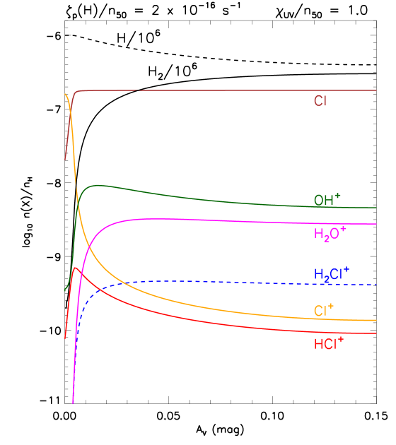
Figure 4: Abundance profiles in an interstellar cloud with properties typical of the diffuse ISM: $\zeta_{p}({\rm H})/n_{50}=2\times 10^{-16}\,\rm s^{-1}$, $\chi_{UV}/n_{50}=1$, and $A_{\rm V}({\rm tot})=0.3$. $A_{\rm V}$ represents the extinction from left edge of the cloud, and cloud center is represented by the right edge of the figure.

In Figure 4, we show the abundance profiles predicted for several species within a diffuse cloud with environmental conditions typical of the diffuse ISM: $\zeta_{p}({\rm H})/n_{50}=2\times 10^{-16}\,\rm s^{-1}$ and $\chi_{UV}/n_{50}=1$. These results plotted here were obtained for a cloud of total visual extinction $A_{V}({\rm tot})=0.3\,\rm mag$, and show the predicted abundances for several species as a function of position in the cloud. Here, the horizontal axis shows the distance from the cloud surface, measured in magnitudes visual extinction, $A_{\rm V}$, and the vertical axis shows the logarithm of the abundances relative to H nuclei. Thus the left edge of the plot represents the irradiated surface of the cloud and the right edge represents its center.

The H₂ abundance rises sharply near the cloud edge, owing to the effects of self-shielding in the dipole-allowed Lyman and Werner band transitions that can lead to photodissociation. This sharp increase is tracked closely by the abundances of OH⁺ and HCl⁺, which are formed in exothermic reactions of H₂ with O⁺ and Cl⁺. As the H₂ fraction increases further, significant abundances of $\rm H_{2}O^{+}$ and $\rm H_{2}Cl^{+}$ appear, the result of further exothermic reactions of H₂ with OH⁺ and HCl⁺. Whereas oxygen is primarily neutral at the cloud surface, chlorine is mainly ionized because its ionization threshold lies (slightly) longward of the Lyman limit. Once the H₂ fraction exceeds $\sim 10^{-3}$, however, chlorine becomes primarily neutral, owing to the reaction of Cl⁺ with H₂ to form HCl⁺. Although the abundances of the oxygen- and chlorine-bearing species are shown in Figure 4 with $A_{V}$ as the independent variable, the fundamental quantity that controls their abundances in this regime is the molecular fraction $2n({\rm H}_{2})/n_{\rm H}$.

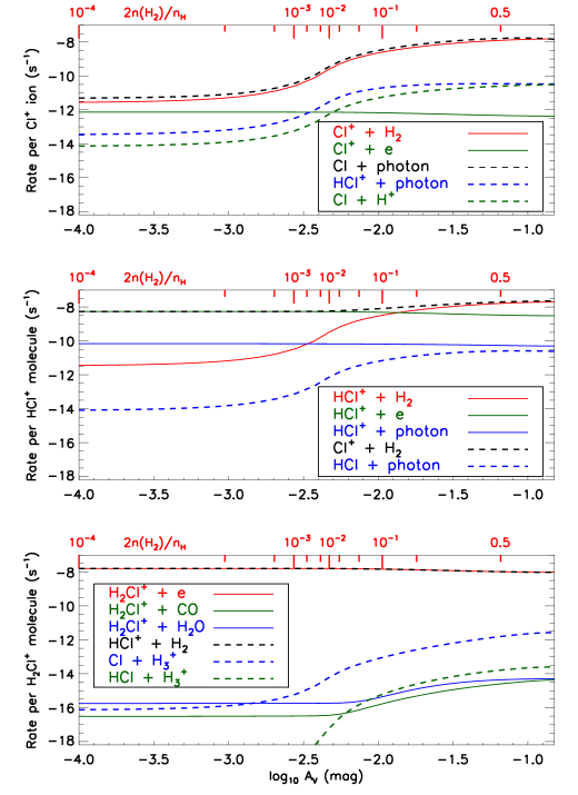
Figure 5: Rates of formation (dashed curves) and destruction (solid curves) per particle for Cl⁺ (top), HCl⁺ (middle), and H₂Cl⁺ (bottom). $A_{\rm V}$, plotted here on a logarithmic scale, represents the extinction from left edge of the cloud, and cloud center is represented by the right edge of the figure. Results are shown for $\zeta_{p}({\rm H})/n_{50}=2\times 10^{-16}\,\rm s^{-1}$, $\chi_{UV}/n_{50}=1$, and $A_{\rm V}({\rm tot})=0.3$.

Figure 5 shows the rates of various reactions in the chemical network. Here, the rates of various destruction and formation processes (solid and dashed curves, respectively) are shown for the three key chlorine-bearing ions: Cl⁺ (top panel), HCl⁺ (middle panel), and H₂Cl⁺. The distance from the cloud surface, again measured in magnitudes of visual extinction, is shown on a logarithmic scale for clarity. Red tick marks at the top of each panel indicate the local molecular fraction, $2n({\rm H}_{2})/n_{\rm H}$. Figure 5 indicates that for the example cloud parameters considered here, the chemistry of these ions is controlled by a relatively small set of processes. Photoionization of Cl dominates the formation of Cl⁺ throughout the cloud, while reaction with H₂ dominates its destruction everywhere. Near the cloud surface, radiative recombination makes a significant additional contribution to the destruction of Cl⁺. The formation of HCl⁺ is dominated by the reaction of Cl⁺ with H₂, and its destruction is dominated by DR (near the surface where $2n({\rm H}_{2})/n_{\rm H}\lower 2.15277pt\hbox{$\;\buildrel<\over{\sim}\;$}0.1$) or reaction with H₂ (in the cloud interior). The latter reaction completely dominates the formation of H₂Cl⁺, for which the only significant destruction process is DR. Beyond the six processes mentioned above – comprising two DR reactions, two hydrogen abstraction reactions, and the photoionization and radiative recombination of Cl – no other process contributes at a level of more than $\sim 2\%$ to the total formation or destruction rate in the case shown here.

5 Discussion

The abundance profiles shown in Figure 4 apply to a single cloud model with given values of $\zeta_{p}({\rm H})/n_{50}$, $\chi_{UV}$, and $A_{\rm V}({\rm tot})$. For this case, and for every other cloud model in the grid we constructed, we may compute the column densities of each species Y, $N({\rm Y})$, for comparison with the measured values.

5.1 Dependence of the $N({\rm H_{2}Cl^{+}})/N({\rm HCl^{+}})$ and $N({\rm H_{2}O^{+}})/N({\rm OH^{+}})$ ratios on the molecular fraction

The chemical network shown in the Figure 3 suggests that the $N({\rm H_{2}Cl^{+}})/N({\rm HCl^{+}})$ ratio, like the $N({\rm H_{2}O^{+}})/N({\rm OH^{+}})$ ratio (e.g. Neufeld et al. 2010), is controlled by the molecular fraction in the ISM. This is demonstrated in Figure 6, where the $N({\rm H_{2}Cl^{+}})/N({\rm HCl^{+}})$ and $N({\rm H_{2}O^{+}})/N({\rm OH^{+}})$ ratios (shown in blue and magenta, respectively) are plotted as a function of $A_{\rm V}({\rm tot})$. All the results shown here were obtained for the same environmental parameters, $\zeta_{p}({\rm H})/n_{50}=2\times 10^{-16}\,\rm s^{-1}$ and $\chi_{UV}/n_{50}=1$. Red tickmarks on the top axis indicate how the average molecular fraction, $2N({\rm H}_{2})/N_{\rm H}$, varies with total visual extinction; and dashed horizontal lines indicate the column density ratios observed for the entire [17,80] km/s velocity interval covered by well-separated foreground gas along the W49N sight-line. As expected, the observed $N({\rm H_{2}X^{+}})/N({\rm HX^{+}})$ ratio generally increases with the molecular fraction for both elements (X = O and X = Cl) However, when compared with the observed ratios, the standard reaction rates (dashed blue curve) yield a clear discrepancy between the predictions for $N({\rm H_{2}O^{+}})/N({\rm OH^{+}})$ (magenta) and those for $N({\rm H_{2}Cl^{+}})/N({\rm HCl^{+}})$. A model with the $2N({\rm H}_{2})/N_{\rm H}$ value $\sim 0.1$ (corresponding to $A_{\rm V}({\rm tot})\sim 0.05$ for these environmental parameters) underpredicts the $N({\rm H_{2}Cl^{+}})/N({\rm HCl^{+}})$ ratio by almost an order-of-magnitude. Moreover, there is no value $A_{\rm V}({\rm tot})$ for which the predicted $N({\rm H_{2}Cl^{+}})/N({\rm HCl^{+}})$ ratio is more than one-third the value observed.

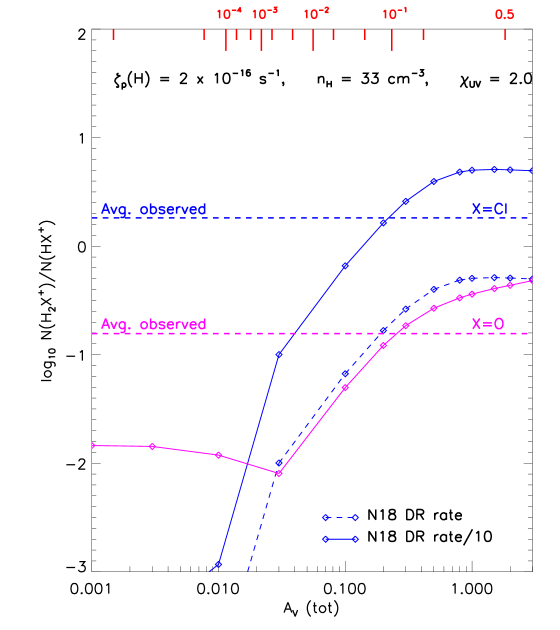
Figure 6: Predicted column density ratios, $N({\rm H_{2}Cl^{+}})/N({\rm HCl^{+}}$ (blue) and $N({\rm H_{2}O^{+}})/N({\rm OH^{+}}$

(magenta), as a function of the total visual extinction through a cloud,$A_{\rm V}({\rm tot})=0.3$. Results are shown for $\zeta_{p}({\rm H})/n_{50}=2\times 10^{-16}\,\rm s^{-1}$ and $\chi_{UV}/n_{50}=1$. Horizontal dashed lines show the values observed for the entire [17,80] km/s velocity interval covered by well-separated foreground gas along the W49N sight-line. Dashed blue curve: predictions with the ${\rm H_{2}Cl^{+}}$ DR rate obtained by N18; solid blue curve: predictions with one-tenth that DR rate (see the text).

The solid blue curve shows $N({\rm H_{2}Cl^{+}})/N({\rm HCl^{+}})$ predictions we obtain with the assumed rate for H₂Cl⁺ DR reduced by a factor 10. Not surprisingly, since DR dominates the destruction of ${\rm H_{2}Cl^{+}}$, the solid blue curve lies a factor of 10 above the dashed blue curve and removes the discrepancy described above. Unless some important ${\rm H_{2}Cl^{+}}$ formation mechanism has been overlooked in our analysis, the observations argue strongly for an H₂Cl⁺ DR rate that is an order-of-magnitude smaller than that adopted in our standard model. The rate coefficient required to match the observed $N({\rm H_{2}Cl^{+}})/N({\rm HCl^{+}})$ ratio is in fact entirely consistent with the measurement of Kawaguchi et al. (2016). The preponderance of the experimental evidence, however, points to a considerably larger DR rate (Geppert et al. 2009, W16, N18) than that measured by Kawaguchi et al. (2016), so the observed $N({\rm H_{2}Cl^{+}})/N({\rm HCl^{+}})$ ratio remains a puzzle. Solutions to this puzzle include the possibility that the DR rate for $N({\rm H_{2}Cl^{+}})$ is anomalously low in its ground rotational state that is predominantly populated at the low density of diffuse interstellar clouds.

5.2 Column densities of molecular ions relative to those of atomic hydrogen

In addition to comparing the observed and predicted values of the ratios $N({\rm H_{2}Cl^{+}})/N({\rm HCl^{+}})$ and $N({\rm H_{2}O^{+}})/N({\rm OH^{+}})$, it is also valuable to consider the column densities of all four molecular ions relative to that of atomic hydrogen. In this part of the analysis, we have fine-tuned the environmental parameters to optimize the fit to $N({\rm HCl^{+}})/N({\rm H})$, $N({\rm OH^{+}})/N({\rm H})$ and $N({\rm H_{2}O^{+}})/N({\rm H})$. Here, we interpolated between grid points and allowed the values of the environmental parameters $\zeta_{p}({\rm H})/n_{50}$ and $\chi_{UV}/n_{50}$ to vary between one-third and three times the “typical” diffuse cloud parameters adopted for Figures 4 – 6. Taking the typical density as $33\,\rm cm^{-3}$ (i.e. $n_{\rm 50}=0.66$) following Wolfire et al. (2003) , we were able to obtain the best simultaneous fit to $N({\rm HCl^{+}})/N({\rm H})$, $N({\rm OH^{+}})/N({\rm H})$ and $N({\rm H_{2}O^{+}})/N({\rm H})$ with an assumed $\zeta_{p}({\rm H})$ of $2.0\times 10^{-16}\,\rm s^{-1}$ and an assumed $\chi_{UV}$ of 2.0. Given these environmental parameters and an assumed total visual extinction of 0.2 mag, we were able to fit the ${\rm HCl^{+}}$, ${\rm OH^{+}}$, and ${\rm H_{2}O^{+}}$ column densities to better than $20\%$. As implied by Section 4.2 above, the ${\rm H_{2}Cl^{+}}$ abundance was, of course, underpredicted by an order-of-magnitude given the standard DR given in Table 2; with the assumed ${\rm H_{2}Cl^{+}}$ DR rate reduced by a factor 10, the column densities of all four molecular ions, relative to that of atomic hydrogen, could be fit simultaneously for entirely reasonable environmental parameters.

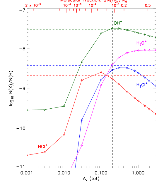
Figure 7: Predicted abundances relative to atomic hydrogen for the optimized environmental parameters $\zeta_{p}({\rm H})=2\times 10^{-16}\,\rm s^{-1}$, $n_{\rm H}=33\,\rm cm^{-3}$, and $\chi_{UV}=2$. The four molecular ion abundances are fit to within $20\%$ for $A_{\rm V}({\rm tot})=0.2$. Here, we adopted an ${\rm H_{2}Cl^{+}}$ DR rate one-tenth that obtained by N18.

The column density ratios $N({\rm HCl^{+}})/N({\rm H})$, $N({\rm H_{2}Cl^{+}})/N({\rm H})$, $N({\rm OH^{+}})/N({\rm H})$ and $N({\rm H_{2}O^{+}})/N({\rm H})$ are shown in Figure 7 as a function of $A_{\rm V}({\rm tot})$. These results apply for the optimal environmental parameters $\zeta_{p}({\rm H})=2.0\times 10^{-16}\,\rm s^{-1}$, $n_{\rm H}=33\,\rm cm^{-3}$ and $\chi_{UV}=2.0$. The dashed horizontal lines indicate the values observed for the entire [17,80] km/s velocity interval covered by well-separated foreground gas along the W49N sight-line; here, the color-coding follows that adopted the theoretical predictions, with results for $N({\rm HCl^{+}})/N({\rm H})$, $N({\rm H_{2}Cl^{+}})/N({\rm H})$, $N({\rm OH^{+}})/N({\rm H})$ and $N({\rm H_{2}O^{+}})/N({\rm H})$ shown respectively in red, blue, green and magenta. The dashed vertical line indicates where the fit is optimized at a molecular fraction $\sim 8\%$ (achieved for $A_{\rm V}({\rm tot})\sim 0.2$ mag).

The satisfactory fit to the $N({\rm HCl^{+}})/N({\rm H})$ described above contrasts with the conclusion reached by DL12 that the observed abundance of ${\rm HCl^{+}}$ exceeded the NW09 model predictions by a factor of 3. Three effects contribute to this difference: (1) the $N({\rm HCl^{+}})$ obtained in the present study is almost $40\%$ smaller than that inferred from the earlier Herschel spectrum; (2) at the kinetic temperature $\sim 120$ K predicted in the gas responsible for the ${\rm HCl^{+}}$ absorption, the ${\rm HCl^{+}}$ DR rate adopted here is $\sim 40\%$ smaller than that adopted by NW09; (3) the optimum fit reported here is obtained for an enhanced (but not unreasonably high) UV field twice the value considered in the models of NW09.

5.3 Variations along the sight-line

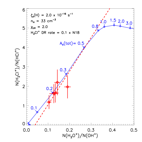
Figure 8: Predicted column density ratios, $N({\rm H_{2}Cl^{+}})/N({\rm HCl^{+}}$ (vertical axis) and $N({\rm H_{2}O^{+}})/N({\rm OH^{+}}$ (horizontal axis), for the optimized environmental parameters. Here, we adopted an ${\rm H_{2}Cl^{+}}$ DR rate one-tenth that obtained by N18. Red points show the observed ratios for the five velocity intervals in which they can be determined reliably. The dashed red line shows the best linear fit to the observed data (with a slope that has a 1 $\sigma$ fractional uncertainty of $\sim 55\%$).

Finally, in Figure 8, we present (red points) the observed $N({\rm H_{2}Cl^{+}})/N({\rm HCl^{+}})$ and $N({\rm H_{2}O^{+}})/N({\rm OH^{+}})$ ratios for the five velocity intervals in Table 2 that are well separated from the source velocity. These are compared with the theoretical predictions obtained for the optimal environmental parameters ($\zeta_{p}({\rm H})=2.0\times 10^{-16}\,\rm s^{-1}$, $n_{\rm H}=33\,\rm cm^{-3}$ and $\chi_{UV}=2.0$) and with the ${\rm H_{2}Cl^{+}}$ DR rate a factor 10 below the standard value. The predictions for this model are represented by the blue locus with values of $A_{\rm V}({\rm tot})$ marked in blue.

As expected the observed $N({\rm H_{2}Cl^{+}})/N({\rm HCl^{+}})$ and $N({\rm H_{2}O^{+}})/N({\rm OH^{+}})$ ratios are positively-correlated with a Pearson correlation coefficient of 0.7 and a best fit linear regression represented by the dashed red line. However, the measured correlation, although suggestive, does not quite reach even a 2 $\sigma$ level of statistical significance.

6 Summary

(1) We have used the GREAT instrument on SOFIA to observe the ${}^{2}\Pi_{3/2}\,J=5/2–3/2$ transition of HCl⁺ near 1444 GHz toward the bright THz continuum source W49N.

(2) The resultant HCl⁺ spectrum reveals absorption by diffuse foreground gas unassociated with the background continuum source.

(3) A comparison with previous Herschel observations of H₂Cl⁺ suggests that the $n({\rm H_{2}Cl^{+}})/n({\rm HCl^{+}})$ abundance ratio varies by a factor of at most 2 along the sight-line.

(4) We have constructed a grid of diffuse cloud models in which the equilibrium abundances of ${\rm HCl^{+}}$ and ${\rm H_{2}Cl^{+}}$ are computed as function of the cloud properties. These models incorporate updates to the rates adopted by NW09 for several significant reactions.

(5) The total column density ratio, $N({\rm H_{2}Cl^{+}})/N({\rm HCl^{+}})$, within the diffuse foreground gas is an order-of-magnitude larger than the predictions of our standard diffuse cloud model. In that model, we adopted a dissociative recombination rate for ${\rm H_{2}Cl^{+}}$ that reflects the values typically obtained in recent laboratory measurements. This discrepant $N({\rm H_{2}Cl^{+}})/N({\rm HCl^{+}})$ ratio suggests that recent laboratory values for the ${\rm H_{2}Cl^{+}}$ or ${\rm D_{2}Cl^{+}}$ DR rates are inapplicable, perhaps because the laboratory studies apply to rotationally-warm molecular ions whereas ${\rm H_{2}Cl^{+}}$ is rotationally-cold in low density interstellar clouds.

(6) For the molecular ions ${\rm HCl^{+}}$, ${\rm OH^{+}}$, and ${\rm H_{2}O^{+}}$, the model predictions can provide a satisfactory fit to the observed column densities along the W49N sight-line. For a cloud density typical of the diffuse ISM, $n_{\rm H}=33\,\rm cm^{-3}$, the optimal parameters are an assumed cosmic-ray ionization rate of $\zeta_{p}({\rm H})=2\times 10^{-16}\,\rm s^{-1}$, an interstellar radiation field $\chi_{\rm UV}$ of 2.0 (i.e. twice the standard value), and a total visual extinction $A_{V}({\rm tot})=0.2$ mag across an individual cloud (leading to a molecular fraction $2N({\rm H}_{2})/N_{\rm H}\sim 8\%$).

References

- Araki et al. (2001) Araki, M., Furuya, T., & Saito, S. 2001, Journal of Molecular Spectroscopy, 210, 132. doi:10.1006/jmsp.2001.8450
- Dagdigian (2019) Dagdigian, P. J. 2019, J. Chem. Phys., 151, 054306. doi:10.1063/1.5115992
- De Luca et al. (2012) De Luca, M., Gupta, H., Neufeld, D., et al. 2012, ApJ, 751, L37. doi:10.1088/2041-8205/751/2/L37 (DL12)
- de Ruette et al. (2016) de Ruette, N., Miller, K. A., O’Connor, A. P., et al. 2016, ApJ, 816, 31. doi:10.3847/0004-637X/816/1/31
- Draine (1978) Draine, B. T. 1978, ApJS, 36, 595. doi:10.1086/190513
- Endres et al. (2016) Endres, C. P., Schlemmer, S., Schilke, P., et al. 2016, Journal of Molecular Spectroscopy, 327, 95. doi:10.1016/j.jms.2016.03.005
- Müller et al. (2005) Müller, H. S. P., Schlöder, F., Stutzki, J., et al. 2005, Journal of Molecular Structure, 742, 215. doi:10.1016/j.molstruc.2005.01.027
- Gerin et al. (2015) Gerin, M., Ruaud, M., Goicoechea, J. R., et al. 2015, A&A, 573, A30. doi:10.1051/0004-6361/201424349 (G15)
- Gerin et al. (2016) Gerin, M., Neufeld, D. A., & Goicoechea, J. R. 2016, ARA&A, 54, 181. doi:10.1146/annurev-astro-081915-023409
- Heays et al. (2017) Heays, A. N., Bosman, A. D., & van Dishoeck, E. F. 2017, A&A, 602, A105. doi:10.1051/0004-6361/201628742
- Heyminck et al. (2012) Heyminck, S., Graf, U. U., Güsten, R., et al. 2012, A&A, 542, L1. doi:10.1051/0004-6361/201218811
- Hollenbach et al. (2012) Hollenbach, D., Kaufman, M. J., Neufeld, D., et al. 2012, ApJ, 754, 105. doi:10.1088/0004-637X/754/2/105
- Kawaguchi et al. (2016) Kawaguchi, K., Muller, S., Black, J. H., et al. 2016, ApJ, 822, 115. doi:10.3847/0004-637X/822/2/115
- Kester et al. (2017) Kester, D., Higgins, R., & Teyssier, D. 2017, A&A, 599, A115. doi:10.1051/0004-6361/201629553
- Kovalenko et al. (2018) Kovalenko, A., Dung Tran, T., Rednyk, S., et al. 2018, ApJ, 856, 100. doi:10.3847/1538-4357/aab106
- Indriolo et al. (2015) Indriolo, N., Neufeld, D. A., Gerin, M., et al. 2015, ApJ, 800, 40. doi:10.1088/0004-637X/800/1/40
- Lis et al. (2010) Lis, D. C., Pearson, J. C., Neufeld, D. A., et al. 2010, A&A, 521, L9. doi:10.1051/0004-6361/201014959
- Lique et al. (2018) Lique, F., Kłos, J., Alexander, M. H., et al. 2018, MNRAS, 474, 2313. doi:10.1093/mnras/stx2907
- Markwardt (2009) Markwardt, C. B. 2009, Astronomical Data Analysis Software and Systems XVIII, 411, 251
- Müller et al. (2001) Müller, H. S. P., Thorwirth, S., Roth, D. A., et al. 2001, A&A, 370, L49. doi:10.1051/0004-6361:20010367
- Neufeld & Wolfire (2009) Neufeld, D. A. & Wolfire, M. G. 2009, ApJ, 706, 1594. doi:10.1088/0004-637X/706/2/1594 (NW09)
- Neufeld et al. (2010) Neufeld, D. A., Sonnentrucker, P., Phillips, T. G., et al. 2010, A&A, 518, L108. doi:10.1051/0004-6361/201014523
- Neufeld et al. (2012) Neufeld, D. A., Roueff, E., Snell, R. L., et al. 2012, ApJ, 748, 37. doi:10.1088/0004-637X/748/1/37
- Neufeld et al. (2015) Neufeld, D. A., Black, J. H., Gerin, M., et al. 2015, ApJ, 807, 54. doi:10.1088/0004-637X/807/1/54 (N15)
- Neufeld & Wolfire (2017) Neufeld, D. A. & Wolfire, M. G. 2017, ApJ, 845, 163. doi:10.3847/1538-4357/aa6d68
- Novotný et al. (2013) Novotný, O., Becker, A., Buhr, H., et al. 2013, ApJ, 777, 54. doi:10.1088/0004-637X/777/1/54 (Errata: ApJ, 795, 176; ApJ, 810, 169) (N13)
- Novotný et al. (2018) Novotný, O., Buhr, H., Geppert, W., et al. 2018, ApJ, 862, 166. doi:10.3847/1538-4357/aacefc (N18)
- Novotný et al. (2019) Novotný, O., Wilhelm, P., Paul, D., et al. 2019, Science, 365, 676. doi:10.1126/science.aax5921
- Sonnentrucker et al. (2015) Sonnentrucker, P., Wolfire, M., Neufeld, D. A., et al. 2015, ApJ, 806, 49. doi:10.1088/0004-637X/806/1/49
- Tran et al. (2018) Tran, T. D., Rednyk, S., Kovalenko, A., et al. 2018, ApJ, 854, 25. doi:10.3847/1538-4357/aaa0d8
- Wakelam et al. (2015) Wakelam, V., Loison, J.-C., Herbst, E., et al. 2015, ApJS, 217, 20. doi:10.1088/0067-0049/217/2/20
- Wiens et al. (2016) Wiens, J. P., Miller, T. M., Shuman, N. S., et al. 2016, J. Chem. Phys., 145, 244312. doi:10.1063/1.4972063 (W16)
- Winkel et al. (2017) Winkel, B., Wiesemeyer, H., Menten, K. M., et al. 2017, A&A, 600, A2. doi:10.1051/0004-6361/201628597
- Wolfire et al. (2003) Wolfire, M. G., McKee, C. F., Hollenbach, D., et al. 2003, ApJ, 587, 278. doi:10.1086/368016