Repulsive Casimir force in stationary axisymmetric spacetimes

Abstract

We study the influence of stationary axisymmetric spacetimes on Casimir energy. We consider a massive scalar field and analyze its dependence on the apparatus orientation with respect to the dragging direction associated with such spaces. We show that, for an apparatus orientation not considered before in the literature, the Casimir energy can change its sign, producing a repulsive force. As applications, we analyze two specific metrics: one associated with a linear motion of a cylinder and a circular equatorial motion around a gravitational source described by Kerr geometry.

1 Introduction

In its original form, the Casimir effect is a quantum phenomenon that arises in the vacuum state of the electromagnetic field in the presence of two neutral metal parallel plates, which impose boundary conditions to the field and produce attraction force between the plates Casimir1 ; Casimir2 . A problem that have attracted a considerable attention in recent years is on which conditions the Casimir force can change from attractive to repulsive, see JeanWi2018 and references therein.

The original attractive force results from a negative Casimir energy. We are especially interested in conditions that can cause a change in the sign of the Casimir energy. It can happen, for example, if a mixed boundary condition (BC) is considered. That is, if Dirichlet or Neumann boundary condition is imposed on both plates, this force is attractive, but it becomes repulsive when fixing a plate with the Dirichlet boundary condition and the other plate with Neumann boundary condition Mostepanenko . In the context of dielectrics materials, Lifshitz predicted in 1956 that the force is attractive for two identical dielectric plates in vacuum Liftshitz2 . A few years later, in 1961, Lifshitz and colleagues generalized this result by considering a medium between the dielectrics plates Liftshitz . As a result, they showed that, if the two plates and the medium have different dielectric constants, the force can become repulsive. Experimental verification of the repulsive Casimir effect was performed at Capasso , by filling the medium with a dielectric liquid, such that the dielectric constants of the three bodies involved in the experiment differ causing a repulsive effect. However, if the two plates have the same dielectric constant, the force is always attractive, regardless the dielectric constant of the medium Liftshitz . Indeed, this last conclusion is a particular result of a non-go theorem Israel , which states that “the Casimir force between two dielectric objects, related by reflection, is attractive.” A possible “loophole” in this theorem may arises when a chiral material is considered as a medium between the plates JeanWi2018 .

In the context of curved spacetimes, Ref. Saharian showed that, in the de Sitter spacetime, for a massive scalar field minimally or conformally coupled to the curvature, the Casimir force can change its sign (for the same BC) if the proper distances between the plates is larger than the curvature radius. We stress that this effect is a consequence of a coupling between the field and the spacetime curvature. Other important result is exposed in the quantum cosmology landscape at Odintsov , where it is shown that the character of being attractive or repulsive Casimir effect is due to the choice of boundary condition related with the dynamic properties of the scale factor in an expanding Friedmann-Robertson-Walker universe.

Other works have considered the Casimir plates immersed in stationary axisymmetric spacetime, with the assumption of the apparatus is very small compared with typical scale on which the metric varies. In this case, the Casimir effect does not break the equivalence principle Milton1 ; Milton2 . The influence of the gravity in the Casimir energy in such scenario was studied for some specific geometries. For example, the Kerr spacetime in Sorge , which study the corrections of the Casimir energy due to the influence of a rotating gravitational source, for a Casimir apparatus describing a circular equatorial orbit. In the aforementioned work, the plates of the apparatus are oriented parallel to the radial coordinate of the gravitational source. The extension for a general stationary spacetime was presented in zhang .

From the above discussion we see that, in a stationary spacetime, the Casimir force is known to change from attractive to repulsive in three cases: for a mixed boundary conditions; with change of the media between the plates (chiral material) and as a consequence of a non-null Ricci scalar curvature. In this work we present a new case when this change can occur. Namely, the change in the sign of the (static) Casimir energy of an identical plates apparatus, for a massive scalar field described by a vacuum solution of a stationary axisymmetric metric. In this case, the Ricci scalar curvature $R$ is zero and the change of sign cannot be associated with direct coupling between the scalar field and $R$. As we will show, in this scenario the Casimir force changes sign when the plates are parallel to the direction of spacetime drag, a case not considered before in the literature. This effect is related with the presence of intrinsic non-diagonal terms in the metric, that is, metrics in which the timelike Killing field fails to be globally hypersurface-orthogonal.

This paper is organized as follows, in Sec. 2 we consider a massive scalar field immersed in a general axisymmetric spacetime, where we solve the Klein-Gordon equation and determine the eigenfrequencies and the normalized solutions. In the Sec. 3 we compute the Casimir energy and present our main result, i.e., the fact that Casimir energy change sign due to the orientation of the apparatus with respect to the drag of the spacetime, we also establish the connection with some already known results for massless case. In the Sections 4 and 5 we apply our approach for two specific stationary background geometries: one with cylindrical symmetry and Kerr metric, respectively. Some final remarks are presented in Sec. 6.

Throughout this paper we use natural units $\hslash=c=G=1$ and we work in signature metric equal to $-2$.

2 Klein-Gordon equation and the frequencies

We are interested in vacuum solutions for massive scalar field inside a Casimir apparatus in an axially symmetric stationary spacetime. Following Sloane and Chandrasekhar Sloane ; chandrasekhar , we demand that such spacetime is stationary, $x^{0}\rightarrow x^{0}+c_{0}$, has axial symmetry, $x^{1}\rightarrow x^{1}+c_{1}$ and is invariant under simultaneous reflection with respect to both $x^{0}$ and $x^{1}$, $x^{0}\rightarrow-x^{0}$ and $x^{1}\rightarrow-x^{1}$. Under these assumptions, the most general line element is given by:

$$ds^{2} =g_{00}\left(dx^{0}\right)^{2}+2g_{01}dx^{0}dx^{1}+g_{11}\left(dx^{1}\right)^{2}$$

$$+g_{22}\left(dx^{2}\right)^{2}+g_{33}\left(dx^{3}\right)^{2}\,,$$ (1)

where the components of the metric tensor depend only on coordinates $x^{2}$ and $x^{3}$. The above metric reflects the non-reversal of time. For a stationary (non-static) spacetime, it is related to the lack of a global time-oriented Killing field (the time-like Killing field is no longer hypersurface orthogonal). A well-known example, which will be analyzed as a special case of our development, is Kerr’s geometry. In this case the cross term, $g_{01}$, is associated with the rotation of the gravitational field source. However, $g_{01}$ is not necessarily related with a rotating source CanSc2003 . Nonrotating vacuum solutions with this term can be used, e.g., to describe superconducting strings with linear momentum GeliTi2000 .

Our goal is to analyze the impact of scalar field mass and the apparatus orientation with respect to the symmetry axis, $x^{1}$, on the Casimir energy. We also compare our results with previous ones, where a specific orientation was chosen for the massless field case Sorge ; zhang . Since energy is a frame-dependent quantity, we must choose the same coordinate frame used in these papers. Namely, a local Cartesian coordinate frame $\left(x,y,z\right)$ comoving with the apparatus. In this frame we have the following line element,

$$ds^{2}=g_{tt}dt^{2}+2g_{tx}dtdx+g_{xx}dx^{2}+g_{yy}dy^{2}+g_{zz}dz^{2}~{},$$ (2)

with determinant $g$,

$$g=g_{yy}g_{zz}\tilde{g}~{},\ \tilde{g}=g_{tt}g_{xx}-g_{tx}^{2}~{}.$$ (3)

A time-dependent transformation applied to the metric (2) may change the notion of energy, making comparisons with the previous results meaningless.

Let us consider a scalar field $\psi\left(x\right)$, with minimal coupling to gravity and mass $m$, that obeys the Klein-Gordon (KG) equation, which in a curved spacetime reads

$$\hat{D}\psi=0~{},\ \hat{D}\equiv\frac{1}{\sqrt{-g}}\partial_{\mu}\sqrt{-g}g^{\mu\nu}\partial_{\nu}+m^{2}~{}.$$ (4)

We call $\hat{D}$ the KG operator. Now, we assume the same approximation made in Sorge ; zhang . Namely, that the apparatus has a small size compared to the scale on which the metric varies. In this situation, one can consider a zero-order expansion of $g_{\mu\nu}$ around the origin. At a first glance, the constant metric approximation on the Klein-Gordon equation makes the problem appear equivalent to the flat case. However, it has been demonstrated by Sorge Sorge and Zhang zhang that this situation is not equivalent to the one in flat space-time. As pointed out in Sorge , this unexpected behavior is due to a symmetry breaking. Namely, for a Casimir apparatus in an axial symmetric metric, with non-diagonal element $g_{tx}$ and the plates orthogonal to the $x$-direction, the associated break of translational invariance induces a distortion in the discretized field modes inside the cavity. In zhang it is shown that, even in this constant metric approximation, the breaking of translational invariance induces non-trivial corrections in Casimir thermodynamic description. For more developments and discussion in this context see ValBeM2019 ; BezCuFM2017 . Our goal is to show that, not only this translational invariance, but also the apparatus orientation with respect to the $x$-direction, influences the discretized field modes inside the cavity. In this zero order expansion of the metric, the KG operator takes the form

$$\hat{D}=g^{tt}\partial_{t}^{2}+2g^{tx}\partial_{t}\partial_{x}+g^{xx}\partial_{x}^{2}+g^{yy}\partial_{y}^{2}+g^{zz}\partial_{z}^{2}+m^{2}~{}.$$ (5)

For constants $K,~{}N~{},\omega$, and considering a solution of the form

$$\psi=Ne^{-i\omega_{n}t}e^{ik_{z}z}\exp\left(iK\omega x\right)f\left(x\right)g\left(y\right)~{},$$ (6)

we have

$$\hat{D} =\left(2g^{tx}K-g^{tt}-g^{xx}K^{2}\right)\omega^{2}+g^{yy}\partial_{y}^{2}-g^{zz}k_{z}^{2}+m^{2}$$

$$+g^{xx}\left[\left(\frac{d}{dx}\ln f\right)^{2}+\frac{d^{2}}{dx^{2}}\ln f\right]$$

$$-2i\omega\left(\frac{d}{dx}\ln f\right)g^{xx}\left(\frac{g^{tx}}{g^{xx}}-K\right).$$ (7)

We can eliminate the imaginary term, linear in $\omega$, by choosing

$$K\equiv\frac{g^{tx}}{g^{xx}}~{}.$$ (8)

Let us assume a local Cartesian frame centered in one of the plates and two different orientations of the Casimir apparatus. The first with the $x$ axis being perpendicular to the plates, which we call the $x$-orientation, note that this is the orientation considered in Ref. Sorge ; zhang . The second one with the $y$ axis being perpendicular to the plates, which we call the $y$-orientation. In what follows we call $\xi$ the coordinate perpendicular to the plates, then we can generally refer to the $\xi$-orientation.

We fix a Dirichlet boundary condition in the first plate. Then we have

$$x\text{-orientation}: f\equiv\sin(k_{x}x)~{},\ g\equiv\exp\left(ik_{y}y\right)~{},$$

$$k_{x}\equiv k_{\xi}~{},\ k_{y}\in\mathbb{R}~{},$$

$$y\text{-orientation}: f\equiv\exp\left(ik_{x}x\right)~{},\ g\equiv\sin\left(k_{y}y\right)~{},$$

$$k_{x}\in\mathbb{R~{}},\ k_{y}\equiv k_{\xi}~{},$$ (9)

where

$$k_{\xi}\equiv\frac{\pi}{L}\left[n-\frac{b}{2}\right]~{},\ n=1,2,\ldots\ ,$$ (10)

and$\ L$ is the (coordinate) distance between the plates. The parameter $b$ fixes the boundary condition on the second plate. For $b=0$, the same condition as Dirichlet is fixed on the second plate, while for $b=1$, one has a Neumann boundary condition on this second plate. The second case ($b=1$) is known as a mixed (or hybrid) boundary condition.

Noting, however, that for both orientations $d^{2}g/dy^{2}=-k_{y}^{2}g$ and that

$$\left(\frac{d}{dx}\ln f\right)^{2}+\frac{d^{2}}{dx^{2}}\ln f=-k_{x}^{2}~{},$$ (11)

we can write

$$\hat{D} =\left[\frac{\left(g^{tx}\right)^{2}}{g^{xx}}-g^{tt}\right]\omega^{2}-g^{xx}k_{x}^{2}$$

$$-g^{zz}k_{z}^{2}-g^{yy}k_{y}^{2}+m^{2}~{}.$$ (12)

Therefore, for both orientations, the spectrum has the form

$$\omega^{2}=\left(g^{xx}k_{x}^{2}+g^{zz}k_{z}^{2}+g^{yy}k_{y}^{2}-m^{2}\right)\left[\frac{\left(g^{tx}\right)^{2}}{g^{xx}}-g^{tt}\right]^{-1}~{}.$$ (13)

Note that, according to (9), $k_{x,y}$ can assume discrete or continuous values.

The solutions must be normalized according to the KG scalar product

$$\left\langle\psi_{m},\psi_{n}\right\rangle=i\int_{\Sigma}\left(\psi_{n}^{\ast}\partial_{\mu}\psi_{m}-\psi_{m}\partial_{\mu}\psi_{n}^{\ast}\right)\,\sqrt{-g_{\Sigma}}\,n^{\mu}~{}d\Sigma~{}.$$ (14)

Where $\Sigma$ is a spacelike Cauchy surface, $g_{\Sigma}$ is the determinant of the metric induced in $\Sigma$ and $n^{\mu}$ is a timelike future-directed unit vector orthogonal to $\Sigma$.

From the arc length, Eq. (2), we can calculate the inverse metric

$$\frac{\partial^{2}}{\partial s^{2}} =\frac{g_{xx}}{\tilde{g}}\frac{\partial^{2}}{\partial t^{2}}-\frac{2g_{tx}}{\tilde{g}}\frac{\partial^{2}}{\partial t\partial x}+\frac{g_{tt}}{\tilde{g}}\frac{\partial^{2}}{\partial x^{2}}$$

$$+\frac{1}{g_{yy}}\frac{\partial^{2}}{\partial y^{2}}+\frac{1}{g_{zz}}\frac{\partial^{2}}{\partial z^{2}}~{}.$$ (15)

From where we can write (13) as

$$\omega^{2}=-g_{tt}\left(\frac{g_{tt}}{\tilde{g}}k_{x}^{2}+\frac{1}{g_{yy}}k_{y}^{2}+\frac{1}{g_{zz}}k_{z}^{2}-m^{2}\right)~{}.$$ (16)

The orthonormal vector to the $\Sigma$ surface can be constructed as

$$\frac{\partial^{2}}{\partial s^{2}} =\frac{1}{\tilde{g}}\left[\left(\sqrt{g_{xx}}\frac{\partial}{\partial t}-\frac{g_{tx}}{\sqrt{g_{xx}}}\frac{\partial}{\partial x}\right)^{2}-\left(\frac{(g_{tx})^{2}}{g_{xx}}-g_{tt}\right)\frac{\partial^{2}}{\partial x^{2}}\right]$$

$$+\frac{1}{g_{yy}}\frac{\partial^{2}}{\partial y^{2}}+\frac{1}{g_{zz}}\frac{\partial^{2}}{\partial z^{2}}~{}.$$ (17)

From this expression, we find

$$n^{\mu}=\left(\sqrt{\frac{g_{xx}}{\tilde{g}}},\frac{g_{tx}}{\sqrt{\tilde{g}g_{xx}}},0,0\right)~{},\ g_{\Sigma}=\frac{g}{g_{tt}}~{}.$$ (18)

As stated, this is a timelike normalized vector, $n^{\mu}n_{\mu}=1$. Using the above $n^{\mu}$ vector in (14), we find the normalization of the solutions of the KG equation

$$\left|N\right|^{2}=-\frac{g_{tt}\sqrt{-g_{tt}g_{xx}g_{yy}g_{zz}}}{g\left(2\pi\right)^{2}L}\left[\omega+\frac{g_{tt}g_{tx}}{\tilde{g}}G_{\xi}k_{x}\right]^{-1}~{},$$ (19)

where

$$G_{\xi}=\begin{cases}0~{},&\text{for }x\text{-orientation}\\ 1~{},&\text{for }y\text{-orientation }\end{cases}~{}.$$ (20)

The main consequence of our development comes from the dependence of the normalization factor, Eq. (19), with the orientation of the plates. In the $x$-orientation, the discrete modes of the field, which do not contribute to the normalization in Eq. (14), are those influenced by the non-diagonal part of the metric. Hence, the non-diagonal metric does not affect the normalization and we have the usual $1/\omega$ dependence, present in the case of the diagonal metric (as well as in the case of the flat space). However, in the $y$-orientation, the continuous modes of the field, which do contribute to the normalization, are influenced by the non-diagonal term in the metric. Therefore $N$ becomes dependent on $g_{tx}$, which, as we will see, also affect the vacuum energy and consequently the Casimir energy.

Regarding this dependence of the normalization with the orientation, it is interesting to note that, in the case of Casimir apparatus in the format of a box (see, e.g. Mostepanenko ), in which case all modes of the field are discrete, the normalization of the field is insensitive to the orientation, because these modes do not contribute to the KG product, regardless of the non-diagonal term in the metric.

3 The vacuum and Casimir energy

In order to compute the Casimir energy, we proceed with the usual techniques of quantum fields in curved spacetimes Birrell . From the energy-momentum tensor for the field,

$$T_{\mu\nu}=\partial_{\mu}\psi\partial_{\nu}\psi^{\ast}-\frac{1}{2}g_{\mu\nu}\left(g^{\rho\sigma}\partial_{\rho}\psi\partial_{\sigma}\psi^{\ast}-m^{2}\left|\psi\right|^{2}\right)~{},$$ (21)

we evaluate the average energy density of the vacuum $\bar{\epsilon}_{vac}$ for the scalar field within the cavity (Casimir’s energy density). This average value reads

$$\bar{\epsilon}_{vac}=\frac{1}{V_{p}}\int dxdydz\sqrt{-g_{\Sigma}}\,\epsilon_{vac}~{},$$ (22)

where

$$V_{P}=\int dxdydz\sqrt{-g_{\Sigma}}~{},$$ (23)

is the proper volume of the cavity, as measured by static observer with four velocity

$$w^{\mu}=\frac{1}{\sqrt{g_{tt}}}\delta^{\mu_{t}}~{},\ g_{tt}>0~{},$$ (24)

while

$$\epsilon_{vac} =w^{\mu}w^{\nu}\left\langle 0\right|T_{\mu\nu}\left|0\right\rangle$$

$$=\left(g_{tt}\right)^{-1}\sum_{n}\int dk_{\alpha}dk_{z}T_{tt}\left[\psi(\vec{k}),\psi^{\ast}(\vec{k})\right]~{}.$$ (25)

The bilinear form $T_{\mu\nu}$ was defined in (21). From now on, we use $\alpha$ to denote the direction orthogonal to the orientation $\xi$ of the plates and $z$ direction, i.e., $\alpha=x$ for the $y$-orientation and $\alpha=y$ for the $x$-orientation.

Our goal is to find the gravity-induced corrections to the vacuum energy density for a scalar quantum field enclosed in the cavity. From (22) and (25) we have,

$$\bar{\epsilon}_{vac}=\frac{1}{g_{tt}}\sum_{n}\int dk_{\alpha}dk_{z}\frac{1}{V_{p}}\int d\Sigma\sqrt{-g_{\Sigma}}T_{tt}\left[\psi(\vec{k}),\psi^{\ast}(\vec{k})\right]~{}.$$ (26)

Using (15) to determine $g^{\rho\sigma}\partial_{\rho}\psi\partial_{\sigma}\psi^{\ast}$, and the solutions (6), with the appropriate choice (9), we find

$$\int_{\Sigma}T_{tt}\sqrt{-g_{\Sigma}}d\Sigma=\int_{z}\int_{\alpha}\int_{\xi}T_{tt}\left(\psi,\psi^{\ast}\right)\sqrt{-g_{\Sigma}}~{}dzd\alpha d\xi~{},$$

$$T_{tt}\left(\psi,\psi^{\ast}\right)=-g_{tt}\left|N\right|^{2}$$

$$\times\left[\sin^{2}\left(k_{\xi}\xi\right)\left(g^{zz}k_{z}^{2}+g^{\alpha\alpha}k_{\alpha}^{2}-m^{2}\right)+\frac{g^{\xi\xi}k_{\xi}^{2}}{2}\right]~{},$$ (27)

where $k_{\alpha}\in\mathbb{R}$ and $\xi$ the variable along the orientation of the plates,

$$x\text{-orientation} :\xi=x\in\left[0,L\right]~{},\ \alpha=y~{},$$

$$y\text{-orientation} :\xi=y\in\left[0,L\right]~{},\ \alpha=x~{}.$$ (28)

Using (16), and evaluating the integrals, we find

$$\frac{1}{V_{p}}\int_{\Sigma}T_{tt}(\psi,\psi^{\ast})\sqrt{-g_{\Sigma}}d\Sigma=\frac{\left|N\right|^{2}\omega^{2}}{2}~{}.$$ (29)

Note that, apart from $N$, the result above does not depend on the orientation of the apparatus. Using (29) in (26) we have

$$\bar{\epsilon}_{vac}=(g_{tt})^{-1}\sum_{n}\int dk_{\alpha}dk_{z}\frac{\left|N\right|^{2}\omega^{2}}{2}~{}.$$ (30)

Substituting now Eq. (19) for the normalization, we obtain,

$$\left|N\right|^{2}\omega^{2}=-\frac{\omega^{2}g_{tt}\sqrt{-g_{tt}g_{xx}g_{yy}g_{zz}}}{g\left(2\pi\right)^{2}L\left(\omega+\frac{g_{tt}g_{tx}}{\tilde{g}}G_{\xi}k_{x}\right)}~{}.$$ (31)

Note that, once $G_{\xi}=0$ for the $x$-orientation, we can write $k_{x}$ or $k_{\alpha}$ in the above equation. We can now determine the average vacuum energy density (26),

$$\bar{\epsilon}_{vac}=-\frac{\sqrt{-g_{tt}g_{xx}g_{yy}g_{zz}}}{2g\left(2\pi\right)^{2}L}\sum_{n}I_{n}~{},$$ (32)

where, making explicit the discrete dependence of $N$ and $\omega$ due to (10), $k_{\xi}=\left(k_{\xi}\right)_{n}$,

$$I_{n}=\int dk_{\alpha}dk_{z}\frac{\omega_{n}^{2}}{\omega_{n}+\frac{g_{tt}g_{tx}}{\tilde{g}}G_{\xi}k_{\alpha}}~{},$$ (33)

and $\omega_{n}$ is given in (16), or (13). Making the variables transformations

$$k_{\alpha}=\sqrt{-\frac{1}{g^{\alpha\alpha}}}k\cos\theta,\quad k_{z}=\sqrt{-g_{zz}}k\sin\theta~{},$$ (34)

we find

$$\omega_{n}^{2}=\left[k^{2}-g^{\xi\xi}k_{\xi}^{2}+m^{2}\right]g_{tt}~{}.$$ (35)

Substituting (35) in (33), and making the integral in $\theta$, we have

$$I_{n}=\frac{\pi}{F^{2}}\sqrt{\frac{g_{tt}g_{zz}}{g^{\alpha\alpha}}}\left[I_{+}+\left(1-F\right)\left(g^{\xi\xi}k_{\xi}^{2}-m^{2}\right)I_{-}\right]~{},$$ (36)

where

$$u=Fk^{2}-g^{\xi\xi}k_{\xi}^{2}+m^{2}~{},\ F=1+\frac{g_{tt}}{g^{\alpha\alpha}}\left(\frac{g_{tx}}{\tilde{g}}G_{\xi}\right)^{2}~{},$$ (37)

and

$$I_{\pm}=\int_{u(0)}^{u(\infty)}u^{\pm 1/2}~{}du~{}.$$ (38)

Both integrals $I_{\pm}$ in (36) diverge, but can be regularized using, for example, zeta regularization zeta . Following the usual method, we start by considering the integral,

$$\int_{u\left(0\right)}^{\infty}u^{-s/2}~{}du=-\frac{u\left(0\right)^{1-s/2}}{1-s/2},\quad\operatorname{Re}\left(s\right)>2~{}.$$ (39)

Where, from (37), we have

$$u\left(0\right)=u_{n}\left(0\right)=-\left(g^{\xi\xi}k_{\xi}^{2}-m^{2}\right)~{},$$ (40)

with $k_{\xi}$ giving in (10). Relaxing for a moment the restriction $\operatorname{Re}\left(s\right)>2$ in (39), we can write (36) as

$$I_{n} =\left[\left(1-F\right)u_{n}\left(0\right)\left.\frac{u_{n}\left(0\right)^{1-s/2}}{1-s/2}\right|_{s=1}-\left.\frac{u_{n}\left(0\right)^{1-s/2}}{1-s/2}\right|_{s=-1}\right]$$

$$\times\frac{\pi}{F^{2}}\sqrt{\frac{g_{tt}g_{zz}}{g^{\alpha\alpha}}}~{},$$ (41)

or yet,

$$I_{n}=\frac{2\pi}{F^{2}}\sqrt{\frac{g_{tt}g_{zz}}{g^{\alpha\alpha}}}\left(\frac{2}{3}-F\right)\left[u_{n}\left(0\right)\right]^{3/2}~{}.$$ (42)

Now we can evaluate the (analytic continuation of the) sum

$$\sum_{n}u_{n}\left(0\right)^{3/2}=\pi^{3}\left[\frac{\sqrt{-g^{\xi\xi}}}{L}\right]^{3}\sum_{n}\left[\left(n+\frac{b}{2}\right)^{2}+q^{2}\right]^{3/2}~{},$$

$$q^{2}=-\frac{L^{2}m^{2}}{\pi^{2}g^{\xi\xi}}~{},$$ (43)

and use the relation zeta

$$\sum_{n=-\infty}^{\infty}\left[\left(n+\frac{b}{2}\right)^{2}+q^{2}\right]^{-s}=\sqrt{\pi}\frac{\Gamma\left(s-\frac{1}{2}\right)}{\Gamma\left(s\right)}$$

$$+\frac{4\pi^{s}}{\Gamma\left(s\right)}q^{\frac{1}{2}-s}\sum_{n=1}^{\infty}\left(-1\right)^{bn}n^{s-\frac{1}{2}}K_{s-\frac{1}{2}}\left(2\pi nq\right)~{},$$ (44)

where $K_{\nu}$ is the modified Bessel function of the second kind. As a result

$$\sum_{n=0}^{\infty}u_{n}\left(0\right)^{3/2} =\frac{3q^{2}\pi}{2}\left[\frac{\sqrt{-g^{\xi\xi}}}{L}\right]^{3}\sum_{n=1}^{\infty}\frac{\left(-1\right)^{bn}}{n^{2}}K_{2}\left(2\pi nq\right)$$

$$+E_{0}\,,$$ (45)

where we use $K_{-2}\left(x\right)=K_{2}\left(x\right)$ and

$$E_{0}=\frac{3}{8}\left[\frac{\pi\sqrt{-g^{\xi\xi}}}{L}\right]^{3}\Gamma\left(-2\right)~{}.$$ (46)

From the asymptotic behavior of the Bessel function AbraSt1072

$$x>>n\Rightarrow K_{n}\left(x\right)\sim\sqrt{\pi}\frac{e^{-x}}{\sqrt{2x}}~{},$$ (47)

we see that the divergent term $E_{0}$ can be associated with the limit $L\rightarrow\infty$ ($q\rightarrow\infty$) and, consequently, it corresponds to the (always divergent) vacuum energy without boundaries. This term must be discounted in the computation of the Casimir energy EliRo1989 . Therefore, discounting $E_{0}$,

$$\sum_{n=0}^{\infty}I_{n} =\frac{3q^{2}\pi^{2}}{F^{2}}\sqrt{\frac{g_{tt}g_{zz}}{g^{\alpha\alpha}}}\left[\frac{\sqrt{-g^{\xi\xi}}}{L}\right]^{3}\left(\frac{2}{3}-F\right)$$

$$\times\sum_{n=1}^{\infty}\frac{\left(-1\right)^{bn}}{n^{2}}K_{2}\left(2q\pi n\right)~{}.$$ (48)

For our consideration of zero order expansion of the metric in the region of the apparatus, the term in brackets from the above equation can be recognized as the proper length $L_{p}$ Sorge ,

$$L_{p}=\int_{0}^{L}\sqrt{-\frac{1}{g^{\xi\xi}}}~{}d\xi=L\sqrt{-\frac{1}{g^{\xi\xi}}}~{}.$$ (49)

Finally, after some manipulations of the elements of the metric, using (49), (48) and (37) in (32), we can write the Casimir energy in the $\xi$-direction as

$$\bar{\epsilon}_{vac}^{\left(\xi\right)}=\left(\frac{\tilde{g}}{g_{tt}g_{xx}}\right)^{\left(4G_{\xi}-1\right)/2}\left(1+3G_{\xi}\frac{g_{tx}^{2}}{\tilde{g}}\right)\mathcal{E}_{m}\mathcal{~{}},$$ (50)

where,

$$\mathcal{E}_{m}=-\frac{m^{2}}{8\pi^{2}L_{p}^{2}}\sum_{n=1}^{\infty}\frac{\left(-1\right)^{bn}}{n^{2}}K_{2}\left(2mL_{p}n\right)~{}.$$ (51)

For the Dirichlet boundary condition ($b=0$) $\mathcal{E}_{m}$ is the well-known Casimir energy for a massive scalar field in flat spacetime, calculated using cutoff or dimensional regularization methods PluMu1986 ; AmbWo1983 . Although the result is not surprising, we have not been able to find this result in the literature for a massive scalar field with mixed boundary conditions ($b=1$).

Equation (50) is our main result. This expression is unchanged by $g_{yy}\leftrightarrow g_{zz}$, indicating that a reorientation of the plates in the $z$-direction reproduces the same result (with $G_{\xi}\equiv G_{y}=1$). Then, while the $x$-orientation has no rotation symmetry, we expect the $y$-orientation to have a symmetry for rotations on the $x$ axis. As highlighted in Sorge the new effects, not present on the flat background, are due to the breaking of $x\rightarrow-x$ symmetry (azimuthal reflection in Kerr geometry). Although diagonalization of Eq. (2) is possible, it would hide this symmetry breaking thus eliminating the new effects originally associated with space-time described by Eq. (1). However, it is possible that the transformation of the spatial coordinates from (1) to (2) is precisely the one that restores this symmetry, diagonalizing the metric of the local Cartesian coordinate frame (e.g., the zero angular momentum observer in Kerr geometry). In this special case, we have

$$g_{tx}=0\Rightarrow\frac{g_{tt}g_{xx}}{\tilde{g}}=1\Rightarrow\bar{\epsilon}_{vac}^{\left(\xi\right)}=\mathcal{E}_{m}\mathcal{~{}},$$ (52)

and all corrections induced by gravity disappear. We will present some concrete examples.

Finally, we highlight the last term in parenthesis in (50). This term could cause a change in the Casimir energy sign, without the insertion of a medium or a change in the boundary condition. A new and unexpected effect. Namely, this change occurs if

$$g_{tx}^{2}<-G_{\xi}\frac{g_{tt}g_{xx}}{2}~{}.$$ (53)

To see that this condition can actually be met, in the next sections we analyze some specific geometries.

This possible change of sign in the Casimir energy can be understood in connection to the dependence of normalization, Eq. (19), on $g_{tx}$ as follows. In the $y$-orientation, the normalization of the field, and consequently the vacuum energy, is affected by the non-diagonal term in the metric. In this case, the balance of energy between continuous and discrete modes inside the apparatus can be modified by the spacetime, changing the sign of the Camisir energy. Conversely, in the $x$-direction, the normalization is not affected by the non-diagonal term, hence the balance of energy inside the apparatus can not be changed.

Now, let’s consider the case without mass. The expressions for the massless scalar field can be obtained from the limit $m\rightarrow 0$. For this goal, we use the behavior of the Bessel functions for small arguments AbraSt1072

$$z\rightarrow 0\Rightarrow K_{\nu}\left(z\right)\sim\frac{1}{2}\Gamma\left(\nu\right)\left(\frac{z}{2}\right)^{-\nu}.$$ (54)

Which implies

$$\mathcal{E}_{m\rightarrow 0}\sim\frac{-1}{16\pi^{2}L_{p}^{4}}\sum_{n=1}^{\infty}\frac{\left(-1\right)^{bn}}{n^{4}}=-\left(-\frac{7}{8}\right)^{b}\frac{\pi^{2}}{1440L_{p}^{4}}~{}.$$ (55)

We can recognize $\mathcal{E}\equiv\mathcal{E}_{m\rightarrow 0}$ as the Casimir energy in the flat spacetime. For $b=1$ we have the $(-7/8)$ factor, resulting a repulsive effect. For the massless case, this sign change, resulting from a mixed boundary condition, is a well-known effect Mostepanenko .

The expression (50) reproduces the results in zhang by choosing the $x$-orientation ($G_{\xi}\equiv G_{x}=0$) and making $m\rightarrow 0$. Unlike flat spacetime, when condition (53) is satisfied, we have a repulsive Casimir force for the same boundary condition in both plates ($b=0$), and an attractive force for a mixed boundary condition ($b=1$).

4 Constant linear momentum cylinder

As a first example, we consider the spacetime external to a distribution of mass-energy with cylindrical symmetry. The distribution is in a non-rotating stationary state of motion along the symmetry axis $\tilde{x}$. Such a system can be described by the metric GeliTi2000

$$ds^{2} =r^{2q_{-}}\cos\left(2k\ln r\right)\left(dt^{2}-d\tilde{x}^{2}\right)-dr^{2}$$

$$-2r^{2q_{-}}\sin\left(2k\ln r\right)dtd\tilde{x}-r^{2q_{+}}d\theta^{2}~{},$$ (56)

where $k$ is a (not necessary positive) constant related with the source momentum, and

$$q_{\pm}=\frac{1}{3}\left[1\pm 2\left(1+3k^{2}\right)^{\frac{1}{2}}\right]~{}.$$ (57)

This metric is stationary but can be static when $k=0$. For $k\neq 0$ it’s an example of a metric satisfying the conditions which define Eq. (1). Possible physical sources for this metric are discussed in GeliTi2000 .

We want to consider a Casimir apparatus moving along the $\tilde{x}$ direction, with constant $r$, $\theta$ and velocity $v=d\tilde{x}/dt$. This apparatus has four-velocity

$$\tilde{w}^{\mu}=S\left(k,r,v\right)\left(1,v,0,0\right)~{},$$ (58)

where

$$S^{-1}\left(k,r,v\right)=r^{q_{-}}\sqrt{\left(v^{2}-1\right)\cos\left(2k\ln r\right)+2v\sin\left(2k\ln r\right)}~{}.$$ (59)

The considered orientations are illustrated in Fig. 1.

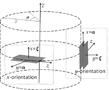
Figure 1: Orientations of the Casimir apparatus for the cylindrically symmetric distribution.

In order to change for a comoving Cartesian reference frame, we first consider the transformation,

$$x^{\prime}=\tilde{x}-vt~{}.$$ (60)

Next, we consider a Cartesian local frame $\left(x,y,z\right)$ attached to the Casimir device and centered on one of the plates. In this frame

$$dx=dx^{\prime},~{}dy=dr~{},~{}dz=rd\theta~{}.$$ (61)

In the comoving frame, the metric assumes the form,

$$g_{tt}=2vg_{tx}-\left(1+v^{2}\right)g_{xx}~{},\ g_{yy}=-1~{},$$

$$g_{tx}=g_{xx}v-r^{2q_{-}}\sin\left(2k\ln r\right)~{},$$

$$g_{xx}=-r^{2q_{-}}\cos\left(2k\ln r\right)~{},\ g_{zz}=-r^{2\left(q_{+}-1\right)}~{}.$$ (62)

In this new metric the apparatus is static with four velocity

$$w^{\mu}=S(k,r,v)(1,0,0,0)~{}.$$ (63)

In addition, for

$$v=v_{d}\equiv-\tan\left(2k\ln r\right)~{},$$ (64)

the three-velocity $\mathbf{w}=0$ is static in coordinates in which the metric locally takes a diagonal form $g_{tx}=0$. It corresponds to an observer (or apparatus) with zero linear momentum. This zero linear momentum observer, with non-vanishing velocity with respect to the original metric (56), represents a form of “frame dragging”, as the one associated with the spacetime of sources endowed with rotation. In other words, using the elements of the original metric (56),

$$v_{d}=-\frac{g_{t\tilde{x}}}{g_{\tilde{x}\tilde{x}}}~{},$$ (65)

is the dragging linear velocity of spacetime.

As pointed out in GeliTi2000 ; ThaMo1998 , for a fixed $\theta$, the Killing vectors $\partial_{t}$ and $\partial_{x}$ may interchange their spacelike/timelike characteristic. Nevertheless, it is possible to define a time orientation at each spacetime point (except $r=0$). Since we consider a fixed $r$, this time orientation does not change. Then, to preserve the time orientation, we must set

$$v_{-}<v<v_{+}~{},\ v_{\pm}=v_{d}\pm\sqrt{v_{d}^{2}+1}~{}.$$ (66)

The $v_{\pm}$ values represent the limit velocities of the apparatus, which we refer to as the ultra-relativistic cases.

Substituting the above components of the metric in (50), and choosing the $x$-orientation for the apparatus ($G_{\xi}=0$), we have

$$\bar{\epsilon}_{vac}^{\left(x\right)}=\mathcal{E}_{m}\sqrt{1-\frac{\left(v-v_{d}\right)^{2}}{v_{d}^{2}+1}}~{}.$$ (67)

While for the $y$-orientation we have

$$\bar{\epsilon}_{vac}^{\left(y\right)}=\mathcal{E}_{m}\frac{v_{d}^{2}+1-3\left(v-v_{d}\right)^{2}}{\left[\left(v_{d}^{2}+1\right)-\left(v-v_{d}\right)^{2}\right]^{\frac{3}{2}}}\sqrt{v_{d}^{2}+1}~{}.$$ (68)

The values coincide for the zero linear momentum

$$v=v_{d}\Rightarrow\bar{\epsilon}_{vac}^{\left(y\right)}=\bar{\epsilon}_{vac}^{\left(x\right)}=\mathcal{E}_{m}~{}.$$ (69)

But it behaves completely differently for all other velocities. In particular, in the ultra-relativistic regimes, $v\rightarrow v_{\pm}$ , we have,

$$v\rightarrow v_{\pm}\Rightarrow\left\{\begin{array}[c]{l}\bar{\epsilon}_{vac}^{\left(x\right)}\rightarrow 0\\ \bar{\epsilon}_{vac}^{\left(y\right)}\rightarrow\left(\pm\right)\infty\end{array}\right.~{},$$ (70)

with the $\left(\pm\right)$ sign for Dirichlet and mixed boundary condition, respectively. While in the $x$-orientation the Casimir energy goes to zero, in the $y$-orientation this energy diverges. Remembering that, as in the Minkowski case, the $\mathcal{E}_{m}$ energy decays with the increase in the mass, in the $y$-orientation a very massive scalar field could still produce a Casimir force. Besides, in the $y$-orientation, the energy, not only diverges, but with a sign opposite to $\mathcal{E}_{m}$. So, without changing the boundary condition, we can change the Casimir force from attractive to repulsive. Namely, the Casimir energy assumes the usual intensity, but with opposite sign when

$$v=\hat{v}_{\pm}\Rightarrow\bar{\epsilon}_{vac}^{\left(y\right)}=-\mathcal{E}_{m}~{}~{},$$

$$\hat{v}_{\pm}=v_{d}\pm\sqrt{\left(2\sqrt{3}-3\right)\left(v_{d}^{2}+1\right)}~{}.$$ (71)

The energy disappear at the velocity

$$v=v_{0\pm}=v_{d}\pm\sqrt{\frac{v_{d}^{2}+1}{3}}\Rightarrow\bar{\epsilon}_{vac}^{\left(y\right)}=0~{}.$$ (72)

Being attractive for $v_{0-}<v<v_{0+}$ and repulsive out this interval.

It is important to note that all values of $\hat{v}_{\pm}$ and $v_{0\pm}$ are in the range (66). This means that the effect of the change in the Casimir force sign cannot be associated with any causal defect in the trajectory, or other prohibited relativistic process.

5 Application for Kerr metric

As a second example, we now apply our result to Kerr’s geometry. A case with more direct applications in physical problems. In this case, the considered orientations are illustrated in Fig. 2.

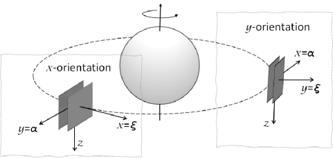
Figure 2: Orientations of the Casimir apparatus for the Kerr metric.

Following Sorge we start with the Kerr metric in the Boyer-Lindquist coordinates,

$$ds^{2} =\left(1-\frac{2Mr}{\Sigma}\right)dt^{2}+2\frac{A}{\Sigma}\omega_{d}\sin^{2}\theta dtd\varphi$$

$$-\frac{\Sigma}{\Delta}dr^{2}-\Sigma d\theta^{2}-\frac{A\sin^{2}\theta}{\Sigma}d\varphi^{2}~{},$$ (73)

where

$$\Sigma=r^{2}+a^{2}\cos^{2}\theta,\hskip 14.22636pt\Delta=r^{2}+a^{2}-2Mr~{},$$

$$A=\left(r^{2}+a^{2}\right)\Sigma+2Mra^{2}\sin^{2}\theta~{},$$ (74)

$a=J/M$ is the Komar angular momentum by unit mass, and

$$\omega_{d}=-\frac{g_{t\varphi}}{g_{\varphi\varphi}}=\frac{2Mar}{A}~{},$$ (75)

is the dragging angular velocity of spacetime. We are interested in circular equatorial orbits, so, as in the previous case, we consider a comoving observer with the apparatus via the transformation,

$$\varphi^{\prime}=\varphi-\Omega t~{},$$ (76)

where $\Omega$ is the angular velocity of the Casimir apparatus. With the transformation (76) the Kerr metric (73) becomes

$$ds^{2} =g_{tt}dt^{2}-\frac{\Sigma}{\Delta}dr^{2}-\Sigma d\theta^{2}-\frac{A\sin^{2}\theta}{\Sigma}d\varphi^{{}^{\prime}2}$$

$$-2\left(\Omega-\omega_{d}\right)\frac{A}{\Sigma}\sin^{2}\theta\,dtd\varphi^{\prime}~{},$$ (77)

where

$$g_{tt}=1-\frac{2A}{\Sigma}\left[\frac{Mr}{A}-\Omega\left(\omega_{d}-\frac{\Omega}{2}\right)\sin^{2}\theta\right]~{}.$$ (78)

For an apparatus in the equatorial orbit ($\theta=\pi/2$, not necessarily geodesic) we can write

$$g_{tt}=\frac{\Delta\Sigma}{A}\left[1-\frac{A^{2}}{\Delta\Sigma^{2}}\left(\Omega-\omega_{d}\right)^{2}\right]~{}.$$ (79)

Allowed observers require $g_{tt}>0$, so

$$\Omega_{-}<\Omega<\Omega_{+}~{},\ \Omega_{\pm}=\omega_{d}\pm\frac{\Sigma\sqrt{\Delta}}{A}~{}.$$ (80)

Now we consider the comoving Cartesian local frame $\left(x,y,z\right)$ attached to the Casimir device and centered on one of the plates,

$$dx=rd\varphi^{\prime},~{}dy=dr,~{}dz=rd\theta~{}.$$ (81)

As a result, the metric (77) takes the form

$$g_{tx} =-\frac{A}{r^{3}}\left(\Omega-\omega_{d}\right)~{},\ g_{xx}=-\frac{A}{r^{4}}~{},$$

$$g_{yy} =-\frac{r^{2}}{\Delta}~{},\ g_{zz}=-1~{}.$$ (82)

Substituting the above components of the metric in (50), and choosing the $x$-orientation ($G_{x}=0$),

$$\bar{\epsilon}_{vac}^{\left(x\right)}=R\left(r;\Omega,M,a\right)\mathcal{E}_{m}~{},$$ (83)

where

$$R\left(r;\Omega,M,a\right) =\sqrt{\frac{g_{tt}g_{xx}}{\tilde{g}}}$$

$$=\left[1-\frac{A^{2}}{r^{4}\Delta}\left(\Omega-\omega_{d}\right)^{2}\right]^{\frac{1}{2}}~{}.$$ (84)

That is the result obtained in Sorge for the massless case, i.e., $\mathcal{E}_{m}=\mathcal{E}_{m\rightarrow 0}$ with $\mathcal{E}_{m\rightarrow 0}$ in (55), where one can find the analysis of $R$ for various parameters ranges.

For the $y$-orientation we have

$$\bar{\epsilon}_{vac}^{\left(y\right)}=\frac{3}{R}\left(1-\frac{2}{3R}\right)\mathcal{E}_{m}~{},$$ (85)

where we used (3). Note that, for $\Omega=\omega_{d}$, called zero-angular-momentum observer (ZAMO), $g_{tx}=0$ and

$$\Omega=\omega_{d}\Rightarrow\bar{\epsilon}_{vac}^{\left(y\right)}=\bar{\epsilon}_{vac}^{\left(x\right)}=\mathcal{E}_{m}~{}.$$ (86)

So (as pointed in Sorge for the $x$-orientation), in this case the symmetry of the spacetime is restored for all orientations. However, out of the ZAMO configuration, the behavior of the Casimir apparatus strongly depends on the orientation,

$$\frac{\bar{\epsilon}_{vac}^{\left(y\right)}}{\bar{\epsilon}_{vac}^{\left(x\right)}}=1-g\left(\delta\right)\left[1+2g\left(\delta\right)\right]~{},$$

$$\delta=\left|\Omega-\omega_{d}\right|\in\left[0,\frac{r^{2}}{A}\sqrt{\Delta}\right)~{},\$$ (87)

where

$$g\left(\delta\right)=-\frac{g_{tx}^{2}}{g_{tt}g_{xx}}=\frac{\left(A\delta\right)^{2}}{\Delta r^{4}-\left(A\delta\right)^{2}}\in\left[0,\infty\right)~{}.$$ (88)

From the above expressions we see that $\bar{\epsilon}_{vac}^{\left(y\right)}\geq\bar{\epsilon}_{vac}^{\left(x\right)}$. This difference in the energy may results in a tendency of the apparatus to assume the lowest energy configuration, i.e., the $x$-orientation, or a torque generating a precession around the $x$ axis.

As a special case we can considered the weak field regime, i.e., let’s keep terms up to first order in the quantities $M/r$ and $a/r$. In this case we can write

$$R=1-x+O\left(x^{2}\right)\Rightarrow R^{-1}\simeq 1+x~{},$$ (89)

which results

$$\frac{\bar{\epsilon}_{vac}^{\left(y\right)}}{\mathcal{E}_{m}}\simeq 1-3x~{}.$$ (90)

Which show that, in the weak field regime, the correction in the $y$-orientation is three times greater than in the $x$-orientation. For the example of a Casimir device resting at the equator of a spinning neutron star, considering $M\simeq 1.4M_{\odot}$, $r\simeq 10^{4}\operatorname{m}$ and $\Omega\simeq 190\operatorname{rad}/\operatorname{s}$, the reference Sorge determines $x=2.3\times 10^{-5}$.

As in the previous example, in the ultra-relativistic regime we have,

$$\Omega\rightarrow\Omega_{\pm}\Rightarrow\left\{\begin{array}[c]{l}\bar{\epsilon}_{vac}^{\left(x\right)}\rightarrow 0\\ \bar{\epsilon}_{vac}^{\left(y\right)}\rightarrow\left(\pm\right)\infty\end{array}\right.~{},$$ (91)

with the $\left(\pm\right)$ sign for Dirichlet and mixed boundary condition, respectively. Again, in the case of the $x$-orientation the Casimir energy goes to zero, as for the Schwarzschild geometry when the orbital motion of the cavity approaches a null geodesic orbit at $r=3M$ Sorge . But, in the $y$-orientation, the energy diverges for a value with a sign opposite to $\mathcal{E}_{m}$. The Casimir force (energy) disappear at the angular velocity

$$\Omega=\Omega_{0\pm}=\omega_{d}\pm\sqrt{\frac{\Delta}{3}}\frac{r^{2}}{A}\Rightarrow\bar{\epsilon}_{vac}^{\left(y\right)}=0~{}.$$ (92)

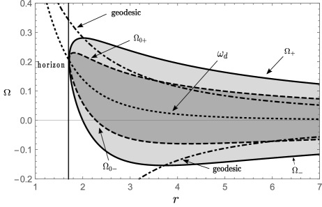
Figure 3: Plot of $\Omega$ with respect to $r$ for $M=1$ and $a=0.7$. The solid lines $\Omega_{\pm}$ represents the ultra-relativistic cases, where the Casimir energy disappear in the $x$-orientation. The dashed line $\Omega_{0\pm}$ are the trajectories where the Casimir energy disappear in the $y$-orientation. The dotted line $\omega_{d}$ the ZAMO trajectory and the dot-dashed line the geodesic trajectories. In the $y$-orientation the energy is negative in the dark gray region and positive in the bright gray region. These grays regions are all the admissible trajectories.

The trajectories for the velocities $\Omega_{0\pm}$ (92) are shown in Fig. 3. In this picture $\Omega_{\pm}$ corresponded to the velocities (80) when the energy tends to zero for the $x$-orientation. In the $x$-orientation the energy is always negative. In the $y$-orientation the energy is negative in the dark gray region and positive in the bright gray region. The energy of both orientations coincides in the ZAMO trajectory $\omega_{d}$. This picture shows also the geodesic trajectories. We have geodesic trajectories where the Casimir force is attractive, repulsive, or null, in the $y$-orientation.

6 Discussion

We studied the Casimir effect in stationary axisymmetric spacetimes, considering two orientations of the plates with respect to the drag of spacetime. We showed that the continuous modes of the field, which contribute to the normalization of the field and, consequently, the Casimir energy, can change the sign of Casimir energy when the plates are perpendicular to the direction of spacetime drag. We have explicitly showed this effect for two examples of such metrics, one associated with a mass-energy with cylindrical symmetry and Kerr spacetime.

Our work reproduce previous results for the massless scalar field in a specific orientation and predict new effects for a massive scalar field. In special, we showed that the geometry of spacetime represents a new mechanism to change the sign of the Casimir energy, even in the absence of gravitational coupling between the scalar and gravitational fields and mixed boundary conditions.

For the Kerr geometry we showed that the Casimir energy for the $y$-orientation is greater than the energy for the $x$-orientation for all admissible circular trajectories, including the geodesics. One can expect that this difference may result in a tendency of the apparatus to assume the lowest energy orientation and align itself in the tangential direction with respect to the object rotation, what can be understood as a quantum compass for spacetime drag. Moreover, in the existence of a torque, that implies in a precession in such direction, in a similar manner that occurs in the Lense-Thirring effect. The effective determination of this new precession effect requires the analyzes of the continuous variation of the orientation, a work in progress.

Although the gravitational verification of this effects requires setups involving the orbits around very massive and rapidly rotating objects (like neutron stars), maybe it can be explored using some hydrodynamic analog of a rotating black hole, as done in hydro2018 to study quasinormal modes of such objects.

References

- (1) H. Casimir, Proc. Kon. Ned. Akad. Wetensch 51, 793 (1948).
- (2) H. Casimir and D. Polder, Phys. Rev. 73, 360 (1948).
- (3) Q. D. Jiang and F. Wilczek, Phys. Rev. B 99, 125403 (2019).
- (4) M. Bordag, G. L. Klimchitskaya, U. Mohideen, and V. M. Mostepanenko, Advances in the Casimir Effect (Oxford University Press, 2008).
- (5) E. M. Lifshitz, Soviet Physics JETP 2, 73 (1956).
- (6) I. E. Dzyaloshinskii, E. M. Lifshitz, and L. P. Pitaevskii, Advan. Phys. 10, 165 (1961).
- (7) J. N. Munday, F. Capasso, and V. A. Parsegian, Nature 457, 170 (2009).
- (8) O. Kenneth and I. Klich, Phys. Rev. Lett. 97, 160401 (2006).
- (9) E. Elizalde, A. A. Saharian, and T. A. Vardanyan, Phys. Rev. D 81, 124003 (2010).
- (10) I. Brevik, K. A. Milton, S. D. Odintsov, and K. E. Osetrin, Phys. Rev. D 62, 064005 (2000).
- (11) K. A. Milton, S. A. Fulling, P. Parashar, A. Romeo, K. V. Shajesh, and J. Wagner, J. Phys. A 41, 164052 (2008).
- (12) S. A. Fulling, K. A. Milton, P. Parashar, A. Romeo, K. V. Shajesh, and J. Wagner, Phys. Rev. D 76, 025004 (2007).
- (13) F. Sorge, Phys. Rev. D 90, 084050 (2014).
- (14) A. Zhang, Phys. Lett. B 125, 773 (2017).
- (15) A. Sloane, Aust. J. Phys. 31, 427 (1978).
- (16) S. Chandrasekhar, The Mathematical Theory of Black Holes (Oxford University Press, 1983).
- (17) F. Canfora and H.-J. Schmidt, Gen. Rel. Grav. 35, 2117 (2003).
- (18) R. J. Gleiser and M. H. Tiglio, Phys. Rev. D 61, 104006 (2000).
- (19) V. B. Bezerra, C. R. Muniz, and H. S. Vieira, Eur. Phys. J. C 79, 879 (2019).
- (20) V. B. Bezerra, M. S. Cunha, L. F. F. Freitas, C. R. Muniz, and M. O. Tahim, Mod. Phys. Lett. A 32, 1750005 (2017).
- (21) N. D. Birrell and P. C. W. Davies, Quantum Fields in Curved Space (Cambridge University Press, 1982).
- (22) E. Elizalde, S. D. Odintsov, A. A. B. Romeo, and S. Zerbini, Zeta Regularization Techniques with Applications (World Scientific, 1994).
- (23) M. Abramowitz and A. Stegun, Handbook of Mathematical Functions with Formulas, Graphs, and Mathematical Tables (National Bureau of Standars, 1972).
- (24) E. Elizalde and A. Romeo, J. Math. Phys. 30, 1133 (1989).
- (25) G. Plunien, B. Muller, and W. Greiner, Phys. Rep. 134, 89 (1986).
- (26) J. Ambjorn and S. Wolfram, Ann. Phys. 147, 1 (1983).
- (27) M. J. Thatcher and M. J. Morgan, Phys. Rev. D 58, 043505 (1998).
- (28) S. Patrick, A. Coutant, M. Richartz, and S. Weinfurtner, Phys. Rev. Lett. 121, 061101 (2018).