A Yang-Baxter integrable cellular automaton
with a four site update rule

Abstract

We present a one dimensional reversible block cellular automaton, where the time evolution is dictated by a period 3 cycle of update rules. At each time step a subset of the cells is updated using a four site rule with two control bits and two action bits. The model displays rich dynamics. There are three types of stable particles, left movers, right movers and “frozen” bound states that only move as an effect of scattering with the left and right movers. Multi-particle scattering in the system is factorized. We embed the model into the canonical framework of Yang-Baxter integrability by rigorously proving the existence of a commuting set of diagonal-to-diagonal transfer matrices. The construction involves a new type of Lax operator.

1 Introduction

Cellular automata are discrete models of classical computation, that can describe complex systems in various domains. They can be applied in physics and chemistry (modeling for example fluid flow, earthquakes, or galaxy formation), but also in biology for the modeling of pattern formation [1, 2]. Their beauty lies in the simplicity of their rules, which can nevertheless lead to very complex behaviour. A famous example is Conway’s Game of Life, which is known to be Turing complete [3].

In physics the cellular automata can play the role of “toy models of nature”: they have the potential to make a bridge between the microscopic and macroscopic physical laws. An important example is the desired rigorous derivation of statistical physics and thermodynamics from the microscopic rules. A special class of models that have been studied for this purpose are the one dimensional reversible cellular automata [4, 5]. The most often studied models are the elementary automata, where the cells are organized in a row, each cell has two states (occupied or empty), the update rules are translationally invariant, and the next state of each cell depends on the current state of the cell and its immediate neighbours. Counting all the possibilities it can be seen that there are $2^{8}=256$ different update rules in this class, and they have been studied and classified in [4, 5]. Reversible models defined on a light cone lattice were afterwards classified and studied in [6]. If cellular automata can serve as toy models for nature, it is very natural to ask whether they can lead to so-called integrable models with non-trivial dynamics. The answer is yes, as we discuss below.

One dimensional integrable models are special systems where the dynamical processes are constrained, leading to completely elastic and factorized scattering [7, 8, 9]. In the quantum mechanical case the wave functions can be constructed with exact methods, leading eventually to the study of the equilibrium and non-equilibrium dynamics of these systems. One of the long standing problems is to compute the macroscopic transport properties from the microscopic dynamics, and this area witnessed tremendous progress since the development of Generalized Hydrodynamics (GHD) [10, 11, 12]. Yet, despite this progress relatively few elements of the theory are rigorously proven (for various partial results see for example [13, 14, 15, 16]). There remains a search for toy models, which are simple enough so that the exact real time dynamics can be computed, but complicated enough in order to have non-trivial interaction effects.

One such toy model is the so-called Rule54 model, which is sometimes also called the Floquet Fredrickson-Andersen (FFA) model, and often claimed to be the simplest interacting integrable model. It is a reversible cellular automaton proposed in [6], where it was shown to have stable particles with soliton-like behaviour. The particles can be right movers or left movers which propagate with a velocity of $\pm 1$. The left-right scattering events are non-trivial: they lead to a displacement of the particle orbits. The Rule54 model has been the subject of active research in the last couple of years, see the recent review [17]. Exact real time evolution in the Rule54 model was computed for special initial states in the recent works [18, 16, 19], leading to a rigorous proof of the predictions of GHD in special cases.

Up to now the Rule54 model remained a somewhat isolated example, residing on the intersection of the worlds of cellular automata and integrable models. Furthermore, the connections with the standard methods of integrability remained obscure. A quantum mechanical deformation of the Rule 54 model was presented in [20], where the so-called Bethe Ansatz solution of the model was also given. Nevertheless it was not known how to embed the model into the famous Yang-Baxter algebra, which is known to be central to integrable models. It is remarkable that the exact computations of [18, 16] did not use any of the standard methods of integrability, and instead they were built on methods developed for “dual unitary quantum gate” models, see [21, 22, 23]. The dual unitary models are not integrable in the traditional sense, but they allow for exact solutions [22, 23].

In this paper it is our goal to construct new cellular automata that are integrable, that show solitonic dynamics, and we make a connection with the canonical methods of quantum integrability.

The possibilities for 2-state cellular automata with strictly local update rules which are also strictly homogeneous in space and time are exhausted by the classifications of [4, 5, 6]. Thus new models can be found if we relax at least some of the requirements. Staying in the realm of 2-state systems one possibility is to look for block cellular automata, where the cells are updated in blocks, and the grouping of the cells into blocks changes periodically with each time step. Such a cellular automaton is a classical version of the brickwork-type local quantum circuits used often in quantum computation. Integrable quantum gate models were studied for example in [24], where a period 2 Floquet cycle of two-site quantum gates was used as an integrable Trotterization of the XXZ Heisenberg chains. It is very natural to attempt to construct block cellular automata using this setup. However, the only deterministic case of the models of [24] is trivial: it leads to simple permutations of quantum spaces and thus to free particle propagation for the resulting cellular automaton. We conclude that new models (with spin-1/2 variables) can be found only if we consider block sizes bigger than 2.

Therefore we consider block cellular automata with block sizes of 3 and 4. This gives us enough freedom to accommodate new and non-trivial solitonic dynamics. The setup we find is similar to that of [24], but now we apply a period 3 Floquet cycle of block updates. We obtain a new integrable cellular automaton, which is perhaps the “next simplest” integrable model after the Rule54 model. The origins of this model lie in the recent works [25, 26, 27, 28], which treated the so-called folded XXZ model, a spin-1/2 chain with remarkably simple dynamical properties. In turn, the folded XXZ model is a special case of the Bariev model [29], which can be interpreted also as a zig-zag spin ladder. As we explain below, our cellular automaton can be regarded as a classical version of the folded XXZ model, and thus of the Bariev model.

In Section 2 we introduce our main model, which uses a 4-site update rule. An alternative version with a 3 site rule (also called the bond model) is introduced in Section 3. We present a quantum mechanical extension (a brickwork-type quantum circuit) in Section 4. The integrability of the models is established in Section 5, where a set of local conserved charges is derived for a certain diagonal-to-diagonal transfer matrix. Our conclusions and a list of open problems is given in Section 6.

2 The cellular automaton: a 4 site model

Consider a spin-1/2 chain of length $L$ with periodic boundary conditions. We require that $L=3k$ with $k\in\mathbb{Z}$. Let us denote the basis states of a local space as ${\left|\circ\right\rangle}$ and ${\left|\bullet\right\rangle}$; they correspond to the up and down spins in the usual $S^{z}$ basis. Correspondingly we introduce the local projection operators onto these basis states:

$$P^{\circ}=\frac{1+\sigma^{z}}{2},\qquad P^{\bullet}=\frac{1-\sigma^{z}}{2}.$$ (2.1)

Here $\sigma^{z}$ is the standard Pauli matrix. We will also use the standard raising and lowering operators with a single matrix element given by the action

$$\sigma^{-}{\left|\circ\right\rangle}={\left|\bullet\right\rangle},\qquad\sigma^{+}{\left|\bullet\right\rangle}={\left|\circ\right\rangle}.$$ (2.2)

Below we introduce quantum circuits, which update the state of the model in discrete time steps. In our main example the update is deterministic. This means that the classical configurations (states of the computational basis) remain classical after each step, and linear combinations do not arise. In this case the quantum circuit model can be interpreted as a cellular automaton.

We start with the unitary quantum gate $U^{(4)}(j)=U^{(4)}_{j,j+1,j+2,j+3}$ which acts on the 4 sites of the segment $[j,\dots,j+3]$. Its explicit form is

$$U^{(4)}(j)=\left(P^{\bullet}_{j}P^{\bullet}_{j+3}+P^{\circ}_{j}P^{\circ}_{j+3}\right)\mathcal{P}_{j+1,j+2}+P^{\bullet}_{j}P^{\circ}_{j+3}+P^{\circ}_{j}P^{\bullet}_{j+3},$$ (2.3)

where $\mathcal{P}_{j+1,j+2}$ is the permutation operator acting on two sites. This is a unitary operator, which is in fact deterministic in the computational basis: acting on any basis state of a segment of 4 sites it results in a single basis state with coefficient 1.

The interpretation of this unitary gate is the following. The outer two spins on site $j$ and $j+3$ are control bits, which control the operation on the inner two bits. If the state of the control bits is the same (be it $\circ$ or $\bullet$) then $U^{(4)}(j)$ permutes the Hilbert spaces on sites $j+1$ and $j+2$. If the two control bits have different values then $U^{(4)}(j)$ acts as identity on the action bits.

The non-zero off-diagonal elements $U^{(4)}(j)$ correspond to the moves shown below:

The action of $U^{(4)}(j)$ leaves all other 4 site combinations invariant.

It is important that $U^{(4)}(j)$ is spin-flip invariant. Furthermore, it is involutive:

$$\left(U^{(4)}(j)\right)^{2}=1.$$ (2.4)

Now we construct the update rules for the cellular automaton. The idea is to construct a period 3 Floquet update rule, such that 3 different update steps are applied periodically. In each update step we identify a subset of the bits as control bits: we designate every third bit as a control bit and apply the 4-site update rule on the pairs of action bits between each pair of neighbouring control bits. In the next time step we shift the selection of the control bits to the right by one site.

This rule can be formalized as follows. We introduce the single step operators $V_{m}$ with $m=1,2,3$ as

$$V_{m}=\prod_{j=1}^{L/3}U^{(4)}(3j+m).$$ (2.5)

Here the $U^{(4)}$-operators are positioned 3 sites apart, which means that two neighbouring $U^{(4)}$ operators share a control bit. The control bits are not changed during the update, thus the operators in the above product commute with each other. The $V_{m}$ operators with different values of $m$ are related by simple translation on the lattice: they merely correspond to shifted choices for the control bits.

Finally we define the period 3 Floquet operator $\mathcal{V}$ as

$$\mathcal{V}=V_{3}V_{2}V_{1}.$$ (2.6)

The time evolution in the cellular automaton is then generated by a repeated action of $\mathcal{V}$ on the chain.

It is important that the operators $V_{m}$ with different values of $m$ do not commute with each other, and it is important to have a pre-defined order of their action. A different ordering leads to a different model.

The single step update rules are reversible, thus the cellular automaton is reversible. Due to the involutive property of the 4-site gate the inverse of the Floquet operator is given by

$$(\mathcal{V})^{-1}=\mathcal{V}^{\prime}=V_{1}V_{2}V_{3}.$$ (2.7)

This ordering of the single step operators corresponds to shifting the control bits to the left after each update step. Thus $\mathcal{V}^{\prime}$ is also the space reflected version of our model, which also implies that the model is $PT$ symmetric.

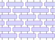
Below we show concrete examples for the dynamics of the model. The time evolution is presented on a two dimensional lattice, where time flows in the vertical direction, such that the bottom line is the initial condition. Sites are indexed such that the leftmost cell corresponds to $j=1$, and the site coordinates increase to the right. We always assume periodic boundary conditions in the horizontal direction, but this is not used explicitly in the examples. The control bits for the update steps are placed according to the formulas (2.6)-(2.5). This means that in the figures the bottom left cell is always a control bit for the corresponding update step. The other control bits are placed on parallel lines in a diagonal direction. We demonstrate this in Figure 1, which shows an empty lattice (all sites unoccupied) with a background coloring of the control bits. We keep this coloring also in the other Figures to be presented below, such that the time evolution can be easily followed/checked by the reader.

Figure 1: An example for the placement of the control bits on a rectangular lattice with $L=9$ and two complete Floquet cycles of length $3$. The vertical axis corresponds to time: each row will depict the state of the cells at a given time. The filled cells are the control bits, that influence the update for the action bits between them. Periodic boundary conditions are understood.

2.1 Dynamics

Now we investigate the dynamics of this cellular automaton. We consider various scenarios (initial states) and look at the outcome of the time evolution. We simply just run the code of the cellular automaton on a periodic lattice and we display the outcome of the dynamics on a two dimensional graph, where the vertical axis corresponds to the time variable. These small runs can be considered as “experiments” with the cellular automaton.

First we consider single particles: we take initial conditions where a single particle is embedded into a vacuum of empty states. Note that due to spin flip invariance the embedding of a single empty state into a fully occupied sea of particles would lead to the same dynamics.

The results of single particle propagation are depicted in Fig. 2. We find that there are two types of particles in the system: right movers and left movers. The position of the particle with respect to the control bits in the given time step decides whether it is a right or a left mover. The rules are the following. Let us assume that at a given time the particle is within the segment $j\dots j+3$ as the unitary gate $U^{(4)}(j)$ is applied. If the particle is at position $j+1$ ($j+2$) then it is moved to the right (left), respectively. If the particle is at site $j$ or $j+4$ then it is not moved in the current step, but it becomes a left mover in the next time step, because it is moved in the next step either by $U^{(4)}(j-2)$ or by $U^{(4)}(j+1)$. Continuing the time evolution we observe that a right mover stays a right mover and it has a constant velocity of 1. Similarly, a left mover stays a left mover, but it moves only in every second step, thus it has an average velocity of $-1/2$.

Figure 2: Propagation of a left mover and a right mover.

Looking at the update rules we also observe that blocks of particles with a minimum length of 2 are frozen, they do not propagate. An example with length 2 is shown below.

These configurations are interpreted as bound states that are not dynamical. The absence of their propagation is a result of the control bits: none of the $U^{(4)}(j)$ gates moves any of the particles in such configurations.

We have thus essentially 3 types of particles in the system with 3 different speeds: right movers with speed 1, left movers with speed -1/2, and bound states with speed 0. It can be seen that bound states with different length behave in the same way, thus there is no need to treat them as separate particle species.

Let us now consider the scattering of particles.

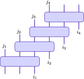
First we look at the scattering of a right mover and a left mover. It is clear from the rules that as the two particles approach each other, there will not be a single time when the two particles occupy neighbouring positions. Any hopping in- and out- of such configuration is forbidden by the control bits. However, there is a non-trivial scattering between the two particles, which is depicted on Fig 3. We see that the right mover eventually continues its orbit, but the left mover suffers a displacement: its outgoing orbit is shifted by one lattice unit to the left and one lattice unit down. This is equivalent to a time delay of $3$ units, which could be considered as a displacement of $\Delta x=-1.5$ due to the average speed of -1/2.

Figure 3: Scattering of a right mover and a left mover.

Let us also consider the scattering of a propagating particle and a bound state. Such processes are depicted on Fig. 4. We observe that the single particles move the frozen bound state by 2 lattice units, always in the direction opposite of the particle propagation. In the case of the right mover we observe that the outgoing orbit is not changed as an effect of the scattering. In the case of the left mover the outgoing orbit suffers a spatial displacement of $\Delta x=-3$. The outcome of the scattering event does not depend on the length of the frozen bound state: the length only affects the duration of the scattering. The explanation for this is simply that as a single particle penetrates the bound state it becomes a hole which can propagate within the bound state with the same fixed velocity, and the time needed to traverse the bound state depends on its size. The scattering displacements are summarized in Table 1.

Figure 4: Scattering of a single particle and a bound state of length 5. Figure on the left: incoming left mover. Figure on the right: incoming right mover.

particle coming	particle coming	$\Delta x_{1}$	$\Delta x_{2}$
from the left	from the right
right mover	left mover	0	-1.5
right mover	bound state	0	-2
bound state	left mover	2	-3

Table 1: A summary of the scattering displacements. Here $\Delta x_{1}$ (or $\Delta x_{2}$) stands for the spatial displacement of the orbit of the particle that was originally incoming from the left (or the right), respectively. The half-integer displacement of $-1.5$ in the case of a left mover signals that in this particular case there is a shift of the orbit in both spatial and temporal directions, resulting in an average spatial displacement that is half-integer.

Let us now turn to multi-particle scattering. A non-trivial multi-particle event can happen only if the incoming particles all have different speed. There are 3 different fixed velocities in the model, thus the only non-trivial case is the 3-body scattering involving a right mover, a bound state, and a left mover. For such processes we find that the scattering displacements are additive, which is a classical version of the “factorized scattering” from quantum integrability. A concrete example for the factorization of the 3-body scattering is shown in Fig 5.

At present we do not have a transparent proof of the factorization, except looking at all the possible scenarios where a non-trivial 3-body effect could happen. It is clear that any violation of the additivity of the displacements can only happen if 3 particles with different velocities occupy positions that are at “interaction distance” with each other. The possibilities for such configurations are limited, and in all cases we found that additivity holds. This property is then extended to all multi-particle scattering events simply because there are only 3 velocities in the model, thus non-trivial 4 body processes are forbidden by kinematics.

Figure 5: An example for a three body scattering, with an incoming right mover from the left, an incoming left mover from the right, and a bound state of length 2. The displacements are found to be additive: The orbit of the right mover is not modified, the position of the bound state is not changed either (displacements due to the left mover and right mover add up to zero), but the left mover suffers a total displacement of -4.5 (once again the half integer replacement is understood as a combined effect of displacement in the horizontal and vertical directions).

3 The bond picture: a 3 site model

An alternative description of the model is achieved by a site-bond transformation that already appeared in the case of the folded XXZ model in [28] (see also [26, 27]). The main observation behind the transformation is that the update rules are spin-flip invariant and they don’t change the state of the control bits. Therefore a simplified rule can be applied by focusing on the bonds between the sites. The idea is to build a new model of length $L$ where the variables are put on the bonds (links) between the original sites. For each configuration we write down a $\circ$ to a given bond if the two cells of the bond have the same state, and a $\bullet$ if they have a different state. Periodic boundary conditions on the original lattice require to have an even number of $\bullet$ states in the bond model. However, it is possible to relax this condition, and we can build an independent bond model where such a condition is not applied.

It can then be seen that each unitary update step $U^{(4)}(j)$ translates into the following three-site unitary $U^{(3)}(j)$ in the bond model:

$$U^{(3)}(j)=P^{\circ}_{j+1}+P^{\bullet}_{j+1}\mathcal{P}_{j,j+2}.$$ (3.1)

Here the middle bit acts as a control bit, which triggers an exchange of the two outer bits. The only transition matrix elements correspond to the moves

All other configurations are left invariant.

In the bond model the time evolution is constructed as

$$\tilde{\mathcal{V}}=\tilde{{V}}_{3}\tilde{{V}}_{2}\tilde{{V}}_{1},$$ (3.2)

where

$$\tilde{V}_{m}=\prod_{j=1}^{L/3}U^{(3)}(3j+m).$$ (3.3)

This time evolution corresponds to a brickwork system of quantum gates depicted in Fig. 6. Notice that now there is no overlap between the gates, as opposed to the four site unitaries of the original representation, whose support overlapped at the control bits.

Figure 6: The system of gates that are used in the 3-site update rules of the bond model. Each brick has three incoming and three outgoing legs, and the action is given by the unitary $U^{(3)}$ defined in the main text. At each step the rows are shifted to the right by one site. The same brickwork structure is used also in the quantum circuit model of Section 4.

The bond model describes the propagation of particles of finite width 2. Once again we find that there are right movers with speed 1 and left movers with an average speed of -1/2. The bound states of the original model are now represented by two single particles that are placed at distance $\ell>1$ from each other. These single particles are interpreted as “domain walls”, as in the case of the folded XXZ model [28]. The domain walls do not propagate on their own, but they are moved by $\pm 2$ sites as an effect of scattering with a dynamical particle. We do not show separate pictures for the time evolution in the bond picture, because they can be obtained easily from the graphs of the original representation by applying the site-bond transformation.

In Section 5 we show that the bond model can be embedded into the canonical algebraic framework of integrability. In order to do this we first introduce a quantum mechanical generalization of the model.

4 Quantum gate model

We consider an extension (or deformation) of the cellular automaton in the bond picture, such that the model becomes fully quantum mechanical. Instead of the deterministic update rule above we introduce a one parameter family of 3-site unitaries given by

$$U^{(3)}_{j,j+1,j+2}(u)=P^{\circ}_{j+1}+P^{\bullet}_{j+1}U^{(2)}_{j,j+2}(u),$$ (4.1)

where now the two-site unitary $U^{(2)}_{j,j+2}(u)$ is defined by its explicit matrix form

$$U^{(2)}_{j,j+2}(u)=\begin{pmatrix}1&0&0&0\\ 0&\text{sech}(u)&i\tanh(u)&0\\ 0&i\tanh(u)&\text{sech}(u)&0\\ 0&0&0&1\\ \end{pmatrix}.$$ (4.2)

Here $\text{sech}(u)=1/\cosh(u)$ and the basis states for the tensor product of the spaces $j$ and $j+2$ are ordered in the standard way of ${\left|\circ\circ\right\rangle},{\left|\circ\bullet\right\rangle},{\left|\bullet\circ\right\rangle},{\left|\bullet\bullet\right\rangle}$. The parameter $u$ is assumed to be a real number. This two-site unitary originates in the $R$-matrix of the XXZ spin chain at the free fermion point [30]. Note that the site in the middle still acts as a control bit and its state is not changed during the update step.

Direct computation shows that

$$U^{(2)}_{j,j+2}(u)U^{(2)}_{j,j+2}(-u)=1,\qquad\left(U^{(2)}_{j,j+2}(u)\right)^{\dagger}=U^{(2)}_{j,j+2}(-u).$$ (4.3)

This confirms the unitarity of $U^{(2)}_{j,j+2}$. The unitarity of the three site gate then follows simply from eq. (4.1).

The three-site gate $U^{(3)}_{j,j+1,j+2}$ can be used to define a one-parameter family of quantum gate models. The time evolution is given by the extension of the formulas (3.2)-(3.3) to include the parameter dependence:

$$\begin{split}\tilde{\mathcal{V}}(u)&=\tilde{{V}}_{3}(u)\tilde{{V}}_{2}(u)\tilde{{V}}_{1}(u),\\ \tilde{V}_{m}(u)&=\prod_{j=1}^{L/3}U^{(3)}_{3j+m,3j+m+1,3j+m+2}(u).\end{split}$$ (4.4)

We refer again to Fig. 6 for a graphical interpretation.

Our main model, the cellular automaton is reproduced in the $u\to\infty$ limit of the quantum gate model. Indeed, in this limit we find

$$\lim_{u\to\infty}U^{(2)}_{j,j+2}(u)=\begin{pmatrix}1&0&0&0\\ 0&0&i&0\\ 0&i&0&0\\ 0&0&0&1\\ \end{pmatrix}.$$ (4.5)

This is identical with the permutation matrix up to the phase factors of $i$ appearing in the exchange transition matrix elements. Thus the three-site unitary (4.1) becomes identical with (3.1) up to these phase factors. It is important, that this operator is deterministic: if the initial condition is a single state from the computational basis, then discrete time evolution will always lead to some other basis state, multiplied with some phase factor. We can then view this motion as purely classical, because there will not be any linear combinations and thus the phases become irrelevant. In other words, the update rules for the mean occupation numbers become identical with the rules of the cellular automaton.

It is also useful to look at the $u\to 0$ limit of the quantum gate model. The two-site and three-site unitaries possess the initial conditions

$$U^{(2)}_{j,j+2}(0)=1,\qquad U^{(3)}_{j,j+1,j+2}(0)=1.$$ (4.6)

Thus at $u=0$ the model becomes completely trivial. The first order Taylor coefficient of the two-site gate gives

$$U^{(2)}_{j,j+1}(u)=1+iu(\sigma^{-}_{j}\sigma^{+}_{j+1}+\sigma^{+}_{j}\sigma^{-}_{j+1})+\mathcal{O}(u^{2}),$$ (4.7)

leading to

$$U^{(3)}_{j,j+1,j+2}(u)=1+iuh_{j,j+1,j+2}+\mathcal{O}(u^{2}),$$ (4.8)

with the Hermitian three-site operator

$$h_{j,j+1,j+2}=\sigma^{-}_{j}P^{\bullet}_{j+1}\sigma^{+}_{j+2}+\sigma^{+}_{j}P^{\bullet}_{j+1}\sigma^{-}_{j+2}.$$ (4.9)

Considering the expansion of the 3-long cycle $\tilde{\mathcal{V}}(u)$ we get

$$\tilde{\mathcal{V}}(u)=1+iuH+\mathcal{O}(u^{2}),$$ (4.10)

where now $H$ is a translationally invariant Hamiltonian

$$H=\sum_{j=1}^{L}h_{j,j+1,j+2}.$$ (4.11)

This is the Hamiltonian of the “folded XXZ model” in the bond model of [28] or in the dual picture of [26, 27]. This model is a special case of the more general Bariev model [29]. Thus the quantum gate model can be regarded as a Trotterization of the folded XXZ and Bariev models. It is remarkable, that this family of quantum models includes the cellular automaton as a special case.

It is important that the spectral parameter dependent Floquet operators $\tilde{\mathcal{V}}(u)$ do not form a commuting family:

$$[\tilde{\mathcal{V}}(u),\tilde{\mathcal{V}}(v)]\neq 0.$$ (4.12)

However, the quantum gate model is still integrable: there is a diagonal-to-diagonal transfer matrix which belongs to a commuting family; this is shown in the next Section. Thus the model can be regarded as an “integrable Trotterization” of the folded XXZ model, and it can be seen as a 3-site analog of the construction of [24], which is an integrable Trotterization of the XXZ spin chain.

For the sake of completeness we also present the quantum gate generalization of the original 4-site update rule of the cellular automaton. Instead of (2.3) we have

$$U^{(4)}(j|u)=\left(P^{\bullet}_{j}P^{\bullet}_{j+3}+P^{\circ}_{j}P^{\circ}_{j+3}\right)U^{(2)}_{j+1,j+2}(u)+P^{\bullet}_{j}P^{\circ}_{j+3}+P^{\circ}_{j}P^{\bullet}_{j+3}$$ (4.13)

with the same two-site unitary given by (4.2). Expanding to first order in $u$ we get

$$U^{(4)}(j|u)=1+iuh_{j,j+1,j+2,j+3}+\mathcal{O}(u^{2})$$ (4.14)

with the four-site Hermitian operator

$$h_{j,j+1,j+2,j+3}=\left(P^{\bullet}_{j}P^{\bullet}_{j+3}+P^{\circ}_{j}P^{\circ}_{j+3}\right)\left(\sigma^{-}_{j+1}\sigma^{+}_{j+2}+\sigma^{+}_{j+1}\sigma^{-}_{j+2}\right).$$ (4.15)

Expanding the $u$-dependent generalization of (2.6) we get

$$\mathcal{V}(u)=1+iuH+\mathcal{O}(u^{2}),$$ (4.16)

where now

$$H=\sum_{j=1}^{L}h_{j,j+1,j+2,j+3}.$$ (4.17)

Apart from a trivial multiplicative normalization this the Hamiltonian of the folded XXZ model treated in [25, 26, 27, 28].

5 Integrability

Now we establish the integrability structure behind the construction, by embedding a certain diagonal-to-diagonal transfer matrix of the bond model into the canonical framework of integrability. As explained in the previous Section, our quantum gate model is a Trotterization of the folded XXZ model, which is a special case of the Bariev model. The algebraic structures behind the Bariev model were worked out in [31, 32]. Our construction to be presented below is independent from these works, but the final result is identical to a specialization of the structures found in [31, 32].

Let us consider the concatenated action of the $U^{(3)}(u)$ gates with some fixed $u$ along a diagonal direction, following the one-site shifts in the definition of (4.4). Formally we have on a chain of length $L$

$$\tau(u)=U^{(3)}_{L-2,L-1,L}\dots U^{(3)}_{3,4,5}(u)U^{(3)}_{2,3,4}(u)U^{(3)}_{1,2,3}(u).$$ (5.1)

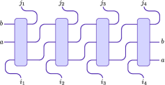
We see that the support for each new gate overlaps with that of the preceding gate on exactly two sites. A graphical representation of such a diagonal-to-diagonal transfer matrix is given in Fig. 7.

The operator $\tau(u)$ is well defined for every finite volume, however, an integrable version is found only in two special situations: either in the infinite volume limit or if we consider periodic boundary conditions along a diagonal direction. We focus on this second possibility. We distribute the incoming and outgoing variables of the transfer matrix such that it will act diagonally from bottom right to the top left, and we apply periodic boundary conditions in a special way: we connect the first two spins at the bottom with the last two spins at the top (see Fig. 7). This is an unphysical boundary condition because it connects spin variables at different times in the lattice. However, this choice leads to a relatively simple embedding of the unitary gates to the standard Yang-Baxter framework of integrability. We give further comments about the utility of the diagonal-to-diagonal transfer matrix at the end of this Section.

Now we present our construction for the transfer matrix. We put forward that the Lax operator and $R$-matrix that we find turn out to be equal to a special case of the same objects given in [31, 32] for the Bariev model. The folded XXZ model corresponds to the special choice $U=\pm 1$ of the Bariev model [29], thus it is very natural that our special solution is included in the general set of results available in the literature . However, we obtained our Lax operator and $R$-matrix using a different route, and for this special model our formulas take simpler form than those of [31, 32]. This is the reason why we chose to publish our derivations.

Let us then consider a tensor product of two auxiliary spaces $a$ and $b$ and a Lax operator $\mathcal{L}_{j,a,b}(u)$ which acts on the tensor product of a physical space $j$ and the two auxiliary spaces. The action of $\mathcal{L}_{j,a,b}(u)$ is given by the three-site unitary above and a permutation which takes care of the proper placement of incoming and outgoing indices for the diagonal-to-diagonal transfer matrix. We get

$$\mathcal{L}_{j,a,b}(u)=\mathcal{P}_{a,b}\mathcal{P}_{j,a}U^{(3)}_{j,a,b}(u).$$ (5.2)

Using this Lax operator we define a new transfer matrix acting on $L$ spins as

$$t(u)=\text{Tr}_{a,b}\left[\mathcal{L}_{L,a,b}(u)\dots\mathcal{L}_{2,a,b}(u)\mathcal{L}_{1,a,b}(u)\right].$$ (5.3)

The trace is taken over both auxiliary spaces. A graphical interpretation of this transfer matrix is given in Fig. 8.

Figure 7: Schematic representation of the diagonal-to-diagonal transfer matrix constructed from three site unitaries. The variables $i_{1},i_{2},\dots$ and $j_{1},j_{2},\dots$ represent the incoming and outgoing indices of the transfer matrix. There are furthermore 4 additional indices corresponding to the first two incoming variables of the first gate, and to the last two outgoing variables of the last gate. Integrability can be established if periodic boundary conditions are applied to these extra 4 variables, see below in Fig. 8.

Figure 8: Schematic representation of the transfer matrix (5.3). Observe that the connectivity of the legs of the quantum gates is the same as in Fig. 7, except for the auxiliary spaces $a$ and $b$ where we apply periodic boundary conditions.

These transfer matrices belong to a commuting family:

$$[t(u),t(v)]=0.$$ (5.4)

This can be proven using the standard steps of the Quantum Inverse Scattering Approach [30]. Let us take two pairs of auxiliary spaces with labels $a,b$ and $c,d$, and let us label the resulting tensor product spaces with $A$ and $B$. Then we can express the two copies of the transfer matrices as

$$\begin{split}t(u)&=\text{Tr}_{A}\left[\mathcal{L}_{L,A}(u)\dots\mathcal{L}_{2,A}(u)\mathcal{L}_{1,A}(u)\right]\\ t(v)&=\text{Tr}_{B}\left[\mathcal{L}_{L,B}(v)\dots\mathcal{L}_{2,B}(v)\mathcal{L}_{1,B}(v)\right],\\ \end{split}$$ (5.5)

where now $\mathcal{L}_{j,A}(u)$ and $\mathcal{L}_{j,B}(v)$ stand for the Lax operator acting on the tensor product of a physical space $j$ and the 4 dimensional auxiliary spaces $A$ and $B$. The commutativity of the transfer matrices can be established if the Lax operators satisfy the so-called RLL relations [30]

$$\begin{split}R_{B,A}(v,u)&\mathcal{L}_{B,j}(v)\mathcal{L}_{A,j}(u)=\mathcal{L}_{A,j}(u)\mathcal{L}_{B,j}(v)R_{B,A}(v,u).\end{split}$$ (5.6)

Here $R_{B,A}(v,u)$ is the so-called $R$-matrix acting on the two auxiliary spaces $A$ and $B$. The spaces $A$ and $B$ are 4 dimensional, therefore $R$ is a matrix of size $16\times 16$.

Consistency of the RLL relations requires that the $R$-matrix satisfies the Yang-Baxter relations, which are operator equations acting on a tensor product of 3 auxiliary spaces:

$$\begin{split}R_{12}(u_{1},u_{2})&R_{13}(u_{1},u_{3})R_{23}(u_{2},u_{3})=\\ &=R_{23}(u_{2},u_{3})R_{13}(u_{1},u_{3})R_{12}(u_{1},u_{2}).\end{split}$$ (5.7)

In our case we find that the Lax operators (5.2) satisfy the RLL relations with the following $R$-matrix :

$$R_{B,A}(v,u)=\begin{pmatrix}E_{11}+E_{44}\rho_{1}&E_{21}&E_{31}+E_{42}\rho_{2}&E_{41}\rho_{5}\\ E_{12}+E_{34}\rho_{2}&E_{22}+E_{44}\rho_{6}&E_{32}\rho_{3}&E_{31}\rho_{4}+E_{42}\rho_{5}\\ E_{13}&E_{23}&E_{33}+E_{44}\rho_{6}&E_{43}\rho_{5}\\ E_{14}\rho_{5}&E_{24}\rho_{5}&E_{12}\rho_{4}+E_{34}\rho_{5}&E_{11}\rho_{7}+(E_{22}+E_{33})\rho_{6}+E_{44}\end{pmatrix}.$$ (5.8)

In the above formula the $R$-matrix is written in a block form, such that it is a $4\times 4$ matrix with respect to the first auxiliary space and the matrix elements written there are operators acting on the second auxiliary space. The operators $E_{\alpha\beta}$ are the elementary matrices with a single matrix element equal to 1 in the row $\alpha$ and column $\beta$. The rapidity dependent functions in the matrix elements above are

$$\begin{split}&\rho_{1}=\tanh(v-u)\tanh(u),\\ &\rho_{2}=i\frac{\tanh(v-u)}{\cosh(u)},\\ &\rho_{3}=\frac{1}{\cosh(v-u)}\left(\frac{\cosh(u)}{\cosh(v)}+\sinh(v-u)\tanh(u)\right),\\ &\rho_{4}=i\frac{\tanh(v-u)}{\cosh(v)},\\ &\rho_{5}=\frac{1}{\cosh(v-u)},\\ &\rho_{6}=i\tanh(v-u),\\ &\rho_{7}=-\tanh(v-u)\tanh(v).\end{split}$$ (5.9)

This $R$-matrix is of non-difference form and it is not symmetric with respect to the two spaces. However, it still satisfies the inversion property

$$R_{B,A}(u,v)R_{A,B}(v,u)=1\quad\text{ with }\quad R_{A,B}(v,u)=\mathcal{P}_{A,B}R_{B,A}(v,u)\mathcal{P}_{A,B}.$$ (5.10)

It also satisfies the so-called regularity condition

$$R_{B,A}(u,u)=\mathcal{P}_{A,B}.$$ (5.11)

The RLL relations and the Yang-Baxter equation can be checked by direct substitution. Afterwards the standard steps of the QISM [30] can be applied to prove the commutativity (5.4).

It is useful to consider the behaviour of $t(u)$ around the initial point $u=0$. The initial condition for the Lax operator follows from (5.2) and (4.6). We get

$$\mathcal{L}_{j,a,b}(u)=\mathcal{P}_{a,b}\mathcal{P}_{j,a}.$$ (5.12)

This is an unusual initial condition, and to our best knowledge it is new. For the transfer matrix it translates into

$$t(0)=\mathcal{U}^{2},$$ (5.13)

where $\mathcal{U}$ is the cyclic shift operator on the finite chain of length $L$. Once again, this initial condition appears to be new: in the standard cases one has simply just $t(0)=\mathcal{U}$. The fact that the transfer matrix describes translation by two sites is very closely tied to the multi-site interactions in the model.

Let us now consider the Taylor expansion of this transfer matrix. Using the expansion (4.8) we obtain the first order terms as

$$t(u)=\mathcal{U}^{2}\left(1+iuH+\mathcal{O}(u^{2})\right),$$ (5.14)

where $H$ is again given by (4.17). Thus the diagonal-to-diagonal transfer matrix also accommodates the “folded XXZ model” (in the bond picture). Due to commutativity of the transfer matrices we can also define further conserved charges by taking the logarithmic derivatives

$$\left.\left(\frac{\partial}{\partial u}\right)^{k}\log(t(u))\right|_{u=0}.$$ (5.15)

Simple arguments show that all of these charges are extensive operators with a short range density, completely analogous to the standard cases. However, the range of these charge densities grows faster than in nearest neighbour interacting chains. The first derivative gives the Hamiltonian which is a 3-site operator, and the next charge is actually a 5-site operator; the range is then increased by 2 with every further derivative.

With this we have obtained an infinite set of local charges for our model. These charges also commute with the Hamiltonian of the “folded XXZ model”. The Bethe Ansatz solution for the eigenstates is already available, it was already given in [26, 27, 28], which diagonalized the Hamiltonian (4.17). Alternatively, the solution could be found by a special limit of the computations given in [29, 31, 32], which could also yield the finite volume transfer matrix eigenvalues.

It is interesting that both $t(u)$ and the 3-cycle operator $\mathcal{V}(u)$ involve the Hamiltonian (4.17) in the first order expansion in $u$ around $u=0$. However, the two operators become different at higher orders in $u$, and only $t(u)$ forms a commuting family.

Let us now return to the original Cauchy problem of the cellular automaton. It is clear that the transfer matrix $t(u)$ can not solve the initial value problem, because it has periodic boundary conditions connecting cells at different time steps. One of the unwanted consequences is that the diagonal-to-diagonal transfer matrix is completely insensitive to the right movers. Those particles actually propagate in parallel with the gates of $t(u)$, and thus the right movers appear as a particle with “infinite velocity” if viewed from the “coordinate frame” of $t(u)$. An analogy is found with relativistic field theories: the right mover is propagating with the “speed of light”, and choosing $t(u)$ as the generator of the dynamics corresponds to choosing light cone coordinates. This is useful only if initial values and boundary values are specified along the light cones, which is a somewhat different setup.

Nevertheless we believe that the Lax operator construction is a clear sign of the algebraic integrability of our model. Perhaps a proper generalization of the Lax operators would actually lead to integrable row-to-row transfer matrices. We leave this as an open problem for future research.

6 Discussion

We presented a new cellular automaton with two different formulations. In the “original picture” the update rule uses two control bits and two action bits, whereas in the “bond picture” only one control bit is used with two action bits. It is important to summarize the connections with existing models in the literature.

First of all, our model can be regarded as a generalization of the Rule54 model, but there are also key differences. Our model has three particle types with three different velocities (left movers, right movers and bound states), and this is richer than simply the left- and right- movers of the Rule54 model. Perhaps our model is the simplest one where factorization of the multi particle scattering can be observed. In the Rule54 model there are no 3 body collisions, but our model has room for such configurations, see for example the scattering event depicted on Fig. 5.

Our model is also similar to various quantum circuit models that appeared in the literature. As explained in Section 4 it can be considered an integrable Trotterization of the “folded XXZ model”, and in this respect it is a 3-site (or 4-site) generalization of the work [24]. Our model is also similar to the dual unitary gate models of [21, 22, 23] and the dual unitary round-a-face models of [33]. These models apply one control bit (dual unitary gate models) or two control bits (dual unitary round-a-face models) for the action of a one site unitary. In our model we have one or two control bits (depending on the formulation) for the action of a two site unitary. Thus we obtained the first member of an even wider class of quantum gate models, potentially including even more integrable models.

One of our key results is the construction of the Lax operator (5.2), which has two new properties as opposed to the standard cases in the literature: it uses two auxiliary spaces (which are coupled), and its initial value at zero rapidity is the cyclic permutation operator acting on the physical space and the two auxiliary spaces. As an effect, the initial value for the resulting transfer matrix is the two-site cyclic shift operator for the underlying spin chain. This leads to a 3-site Hamiltonian, and an infinite family of conserved charges, such that there is no 2-site operator commuting with them. Nevertheless the charges are translationally invariant, with respect to single site shifts. Similar constructions already appeared in the literature. The most important example is the algebraic treatment of the Bariev model [31, 32], which actually includes our solution in a special limit. Other examples for similar constructions are zig-zag spin ladders or coupled XXZ spin chains (see for example [34, 35, 36]). Nevertheless the formalism presented in this paper seems to be new, and for this particular model our formulas are more transparent than those of [31, 32].

Let us now discuss some of the open questions. First of all, it would be important to find out whether the row-to-row transfer matrix $\mathcal{V}(u)$ possesses any integrability properties. Even though $[\mathcal{V}(u),\mathcal{V}(v)]\neq 0$ it is still possible that there is a multi-parametric extension of these transfer matrices, such that a restricted commutativity would still hold within the larger family. This would then extend the commutativity properties of the transfer matrices in [24]. However, at present it is not clear whether such a structure should be expected, and it would be desirable to study the level statistics $\mathcal{V}(u)$ to get a working hypothesis about its integrability. We remind that the diagonal-to-diagonal transfer matrix $t(u)$ can not handle the Cauchy problem of the cellular automaton (see the discussion at the end of the previous Section), and this motivates further study of the row-to-row transfer matrix $\mathcal{V}(u)$.

It would be interesting to determine the large scale transport properties of the present models. We expect to find ballistic transport with diffusive corrections, just like in the Rule54 model [37, 38]. As argued above, our cellular automaton is perhaps the simplest model with factorized multi-particle scattering, therefore it could be used as a further testing ground for the predictions of GHD.

Finally, perhaps the most interesting question is, what type of new integrable models we can still obtain with the present algebraic construction. In this work we used one or two control bits and the $R$-matrix of the XX chain for the two-site unitary $U^{(2)}(u)$. An obvious idea is to use the known $R$-matrix of the XXZ chain for the same purpose. This will not give us a new cellular automaton, but it will result in new integrable spin chains (or quantum gate models), which can be considered as “hard rod deformations” of the XXZ spin chains. This will be presented in a separate publication in collaboration with other researchers.

Acknowledgments

We are grateful to Tamás Gombor, Arthur Hutsalyuk, Yunfeng Jiang, Tomaž Prosen, Eric Vernier and Lenart Zadnik for useful discussions. In particular we thank Arthur Hutsalyuk for providing us the $R$-matrix in eq. 5.8, and Tamás Gombor for checking some of the formulas and for his help with some of the Figures in this document. We are grateful to Lenart Zadnik for referring us to the papers [31, 32] which treated the algebraic structures behind the Bariev model.

References

- [1] M. Mitchell, Computation in Cellular Automata: A Selected Review, ch. 4, pp. 95–140. John Wiley & Sons, Ltd, 1998.
- [2] S. Wolfram, A New Kind of Science. Wolfram Media, 2002.
- [3] P. Rendell, Turing Machine Universality of the Game of Life. Springer International Publishing, 2016.
- [4] S. Wolfram, “Statistical mechanics of cellular automata,” Rev. Mod. Phys. 55 (1983) 601–644.
- [5] S. Takesue, “Reversible Cellular Automata and Statistical Mechanics,” Phys. Rev. Lett. 59 (1987) 2499–2502.
- [6] A. Bobenko, M. Bordemann, C. Gunn, and U. Pinkall, “On two integrable cellular automata,” Comm. Math. Phys. 158 (1993) no. 1, 127 – 134.
- [7] B. Sutherland, Beautiful Models. World Scientific Publishing Company, 2004.
- [8] R. J. Baxter, Exactly solved models in statistical mechanics. London: Academic Press Inc, 1982.
- [9] G. Mussardo, “Off-critical statistical models: Factorized scattering theories and bootstrap program,” Phys. Rept. 218 (1992) 215–379.
- [10] O. A. Castro-Alvaredo, B. Doyon, and T. Yoshimura, “Emergent Hydrodynamics in Integrable Quantum Systems Out of Equilibrium,” Phys. Rev. X 6 (2016) no. 4, 041065, arXiv:1605.07331 [cond-mat.stat-mech].
- [11] B. Bertini, M. Collura, J. De Nardis, and M. Fagotti, “Transport in Out-of-Equilibrium XXZ Chains: Exact Profiles of Charges and Currents,” Phys. Rev. Lett. 117 (2016) no. 20, 207201, arXiv:1605.09790 [cond-mat.stat-mech].
- [12] A collection of review articles in the topic of GHD will appear in the near future in a Special Issue of J. Stat. Mech.
- [13] B. Doyon, “Hydrodynamic projections and the emergence of linearised Euler equations in one-dimensional isolated systems,” arXiv e-prints (2020) , arXiv:2011.00611 [math-ph].
- [14] E. Granet and F. H. L. Essler, “Systematic strong coupling expansion for out-of-equilibrium dynamics in the Lieb-Liniger model,” arXiv e-prints (2021) , arXiv:2102.09987 [cond-mat.stat-mech].
- [15] M. Borsi, B. Pozsgay, and L. Pristyák, “Current operators in integrable models: A review,” arXiv e-prints (2021) , arXiv:2103.12160 [cond-mat.stat-mech].
- [16] K. Klobas and B. Bertini, “Exact relaxation to Gibbs and non-equilibrium steady states in the quantum cellular automaton Rule 54,” arXiv e-prints (2021) , arXiv:2104.04511 [cond-mat.stat-mech].
- [17] B. Buča, K. Klobas, and T. Prosen, “Rule 54: Exactly solvable model of nonequilibrium statistical mechanics,” arXiv e-prints (2021) , arXiv:2103.16543 [cond-mat.stat-mech].
- [18] K. Klobas, B. Bertini, and L. Piroli, “Exact Thermalization Dynamics in the “Rule 54” Quantum Cellular Automaton,” Phys. Rev. Lett. 126 (2021) 160602, arXiv:2012.12256 [cond-mat.stat-mech].
- [19] K. Klobas and B. Bertini, “Entanglement dynamics in Rule 54: exact results and quasiparticle picture,” arXiv e-prints (2021) , arXiv:2104.04513 [cond-mat.stat-mech].
- [20] A. J. Friedman, S. Gopalakrishnan, and R. Vasseur, “Integrable Many-Body Quantum Floquet-Thouless Pumps,” Phys. Rev. Lett. 123 (2019) 170603, arXiv:1905.03265 [cond-mat.stat-mech].
- [21] P. Kos, M. Ljubotina, and T. Prosen, “Many-Body Quantum Chaos: Analytic Connection to Random Matrix Theory,” Phys. Rev. X 8 (2018) no. 2, 021062, arXiv:1712.02665 [nlin.CD].
- [22] B. Bertini, P. Kos, and T. Prosen, “Exact Correlation Functions for Dual-Unitary Lattice Models in 1+1 Dimensions,” Phys. Rev. Lett. 123 (2019) no. 21, , arXiv:1904.02140 [cond-mat.stat-mech].
- [23] L. Piroli, B. Bertini, J. I. Cirac, and T. Prosen, “Exact dynamics in dual-unitary quantum circuits,” Phys. Rev. B 101 (2020) no. 9, 094304, arXiv:1911.11175 [cond-mat.stat-mech].
- [24] M. Vanicat, L. Zadnik, and T. Prosen, “Integrable Trotterization: Local Conservation Laws and Boundary Driving,” Phys. Rev. Lett. 121 (2018) no. 3, 030606, arXiv:1712.00431 [cond-mat.stat-mech].
- [25] Z.-C. Yang, F. Liu, A. V. Gorshkov, and T. Iadecola, “Hilbert-Space Fragmentation from Strict Confinement,” Phys. Rev. Lett. 124 (2020) no. 20, 207602, arXiv:1912.04300 [cond-mat.str-el].
- [26] L. Zadnik and M. Fagotti, “The Folded Spin-1/2 XXZ Model: I. Diagonalisation, Jamming, and Ground State Properties,” SciPost Phys. Core 4 (2021) 10, arXiv:2009.04995 [cond-mat.stat-mech].
- [27] L. Zadnik, K. Bidzhiev, and M. Fagotti, “The Folded Spin-1/2 XXZ Model: II. Thermodynamics and Hydrodynamics with a Minimal Set of Charges,” SciPost Phys. 10 (2021) 99, arXiv:2011.01159 [cond-mat.stat-mech].
- [28] B. Pozsgay, T. Gombor, A. Hutsalyuk, Y. Jiang, L. Pristyák, and E. Vernier, “An integrable spin chain with Hilbert space fragmentation and solvable real time dynamics,” arXiv e-prints (2021) , arXiv:2105.02252 [cond-mat.stat-mech].
- [29] R. Z. Bariev, “Integrable spin chain with two- and three-particle interactions,” Journal of Physics A: Mathematical and General 24 (1991) no. 10, L549–L553.
- [30] V. Korepin, N. Bogoliubov, and A. Izergin, Quantum inverse scattering method and correlation functions. Cambridge University Press, 1993.
- [31] H.-Q. Zhou, “Quantum integrability for the one-dimensional Bariev chain,” Phys. Lett. A 221 (1996) no. 1, 104–108.
- [32] M. Shiroishi and M. Wadati, “Integrability of the one-dimensional Bariev model,” J. Phys. A 30 (1997) no. 4, 1115–1133.
- [33] T. Prosen, “Many Body Quantum Chaos and Dual Unitarity Round-a-Face,” arXiv e-prints (2021) , 2105.08022 [cond-mat.stat-mech].
- [34] V. Popkov and A. Zvyagin, ““Antichiral” exactly solvable effectively two-dimensional quantum spin model,” Phys. Lett. A 175 (1993) no. 5, 295–298.
- [35] H. Frahm and C. Rödenbeck, “Integrable models of coupled Heisenberg chains,” Europhys. Lett. 33 (1996) no. 1, 47–52, arXiv:cond-mat/9502090 [cond-mat].
- [36] A. A. Zvyagin, “Bethe ansatz solvable multi-chain quantum systems,” J. Phys. A 34 (2001) no. 41, R21–R53.
- [37] K. Klobas, M. Medenjak, T. Prosen, and M. Vanicat, “Time-dependent matrix product ansatz for interacting reversible dynamics,” Comm. Math. Phys. 371 (2019) no. 2, 651–688, arXiv:1807.05000.
- [38] S. Gopalakrishnan, D. A. Huse, V. Khemani, and R. Vasseur, “Hydrodynamics of operator spreading and quasiparticle diffusion in interacting integrable systems,” Phys. Rev. B 98 (2018) no. 22, 220303, arXiv:1809.02126 [cond-mat.stat-mech].