High Resolution Time-Frequency Generation
with Generative Adversarial Networks

Abstract

Signal representation in Time-Frequency (TF) domain is valuable in many applications including radar imaging and inverse synthetic aparture radar. TF representation allows us to identify signal components or features in a mixed time and frequency plane. There are several well-known tools, such as Wigner-Ville Distribution (WVD), Short-Time Fourier Transform (STFT) and various other variants for such a purpose. The main requirement for a TF representation tool is to give a high-resolution view of the signal such that the signal components or features are identifiable. A commonly used method is the reassignment process which reduces the cross-terms by artificially moving smoothed WVD values from their actual location to the center of the gravity for that region. In this article, we propose a novel reassignment method using the Conditional Generative Adversarial Network (CGAN). We train a CGAN to perform the reassignment process. Through examples, it is shown that the method generates high-resolution TF representations which are better than the current reassignment methods.

I Introduction

Joint Time-Frequency (TF) representation of a signal reveals many features which are valuable in many applications including radar imaging [1] and inverse synthetic aperture radar (ISAR) [2] in which a high-resolution joint-TF analysis is necessary to obtain a focused image of the target. TF representation is also valuable in many sound classification [3] and recognition [4] applications. In many Convolutional Neural Network (CNN) sound applications [5], TF representations boosts the performance of the Network.

The classical tool for the TF representation is the Wigner-Ville Distribution(WVD) [6]. Though it has many good features, it suffers from cross terms which makes the readability of the TF distribution difficult and hard to interpret. Another well-known tool is the Short Time Fourier Transform (STFT) [7]. STFT does not produce any the cross terms but deteriorates the resolution of the signal. There are various other derivatives of the WVD which are named as the Cohen’s Class of distributions. In addition, there are other representations which process smoothed versions of WVD by a method called as the reassignment [8] to obtain high resolution.

In this article a high resolution TF representation is obtained by using Generative Adversarial Networks (CGAN) [9], in particular by using a Conditional GAN (CGAN) implementation pix2pix [10] developed for general image to image transformation applications.

II TIME FREQUENCY REPRESENTATIONS

The classical tool for the TF analysis is the Wigner-Ville Distribution (WVD)[6]. WVD of a signal $x(t)$ is given by,

$$W_{x}(t,f)=\int_{-\infty}^{+\infty}x(t+\tau/2)x^{*}(t-\tau/2)e^{-j2\pi f\tau}d\tau.$$ (1)

WVD has many good features, such as high resolution and is a real valued distribution but due to its quadratic nature it produces unwanted artifacts, named as cross terms, on the TF plane. This makes the readability of different signal parts on TF plane difficult. A generalization of the WVD is the Cohen’s Class [11] distribution given by,

$$P_{x}(t,f)=\iint_{-\infty}^{+\infty}A_{x}(\theta,\tau)\Phi(\theta,\tau)e^{-j2\pi(\theta t+f\tau)}d\theta d\tau.$$ (2)

where $A_{x}(\theta,\tau)$ is the ambiguity function (AF) of the signal $x(t)$ and has a two-dimensional (2D) Fourier transform relation with WVD. $\Phi(\theta,\tau)$ is the kernel of the distribution and has the time-frequency shaping or smoothing effect on $W_{x}(t,f)$. A proper kernel can attenuate the cross terms and produce high resolution distribution [12, 13, 14].

Another classical tool for the TF analysis is the Short-Time Fourier Transform (STFT) given by

$$STFT_{x}(t,f)=\int_{-\infty}^{+\infty}x(\tau)w^{*}(\tau-t)e^{-j2\pi f\tau}d\tau,$$ (3)

where, $w(t)$ is the time domain window having the smoothing effect on frequency domain. Spectrogram given by $S_{x}(t,f)=|STFT_{x}(t,f)|^{2}$ is a member of Cohen’s Class and depending on the length of the window, can attenuate the cross terms. But there is a trade off between the cross term suppression and the TF resolution or localization.

As a remedy to the resolution problem, the reassignment method is developed [8]. In reassignment, the value of a smoothed version, $P_{x}(t,f)$ of WVD is moved to a new location $(\hat{t},\hat{f})$ which is the center of the gravity of the signal energy distributed around $(t,f)$. In this way, a better localization is obtained. In Figure 1 the ideal TF, the WVD, a smoothed version of WVD, called Smoothed Pseudo WVD (SPWVD) and the reassignment of SPVWD (RSPWVD) are shown for a sample signal. As can be seen WVD is not able to reveal the three TF signal components. The SPWVD is able to show them but with a reduced resolution. But RSPWVD substantially reduces the cross terms and it also achieves high resolution or localization. Though the reassignment has high localization, it may deviate from the desired or ideal TF. In fact, at some $(t,f)$ points it may exhibit peaks which do not explain the underlying signal. This is caused by the nonlinear reassignment operation.

(a) Ideal TF

(b) WVD

(c) SPWVD

(d) RSPWVD

Figure 1: a) TF representation of a signal with ideal, b) WVD, c) SPWVD and d) RSPWVD, respectively.

III GENERATIVE ADVERSARIAL NETWORKS

Convolutional Neural Networks (CNN)s have revolutionized computer vision and image classification fields [15]. Most image processing applications can be regarded as a mapping from an input image to an output image. Until recent advances in (CNN) area, the image mapping tasks have been performed by classical image processing tools [16, 17]. Convolutional autoencoders and Generative Adversarial Networks (GANs)[9] have been successfully used in image generation prediction applications [18]. In general, autoencoder type CNNs are trained to minimize a given cost function which determines whether an image generated by CNN is close to a desired or a given label image [15]. The quality of output or predicted image is heavily dependent on the selected cost function. Autoencoders trained with Euclidean ($\ell^{2}$) distance, or their regularized versions with the $\ell^{1}$ norm produce blurred predictions [19]. Therefore, selecting a proper cost function is crucial in CNN based image prediction problems. On the other hand, Generative Adversarial Networks (GAN) [9] have a different structure with a novel cost function and they achieve sharp image reconstructions. GANs have two competing networks. The Discriminator ($D$) network tries to determine if its input is real or artificially generated by the Generator ($G$) network. GANs are trained with a min-max optimization method given by [9]

$$\min_{G}\max_{D}V(D,G) =E_{Y\sim p_{Y}(Y)}[\log D(Y)]$$

$$+E_{Z\sim p_{Z}(Z)}[\log(1-D(G(Z)))].$$ (4)

where $Y$ represents an actual data sample (image) and $Z$ is a random vector representing the latent space whose probability distribution function (pdf) $p_{Z}(Z)$ is given a priori. The generator network $G$ is trained to generate an image according to its input vector $Z$. $E_{Y\sim p_{Y}(Y)}$ and $E_{Z\sim p_{Z}(Z)}$ are the expectation over data samples and the random variable $Z$, respectively. The network is trained in an alternating manner. In one turn $D$ is fixed and parameters of $G$ are trained, in the next round, $G$ is fixed and $D$ is trained. The aim of GAN is to estimate the pdf $p_{Y}(Y)$ of data so that, when fed by a random variable $Z$ the samples generated by $G$ are indistinguishable from actual data samples. In other words, the generator is trained to fool the discriminator. On the other hand, the discriminator is trained not to be fooled. The beauty of GANs come from the definition of their cost function. Rather than measuring the distance between the desired and the generator ($G$) output with a predefined cost function the generator output is classified either as real or fake via the discriminator network $D$ . In this way, the parameters of of the generator network are ”learned” during training process.

A variant of the original GAN, which has proved success in image prediction and generation, is the Conditional GAN (CGAN). In CGANs the generation process is based on a given condition. During training, together with the random variable $Z$, an input $X$, which define a condition on what is to be generated, is fed both to the generator and the discriminator. In this training approach, the generator is able to generate samples which are restricted by the condition $X$. In CGAN, rather than the prior distribution $p_{Y}(Y)$, the conditional pdf $p_{Y|X}(Y|X)$ is estimated.

IV TF GENERATION WITH CGAN

In this section, we consider the TF plots as two-dimensional images and generate reassigned TF plots from SPWVD distributions using CGANs. Even though the aim of CGAN is to estimate a conditional pdf $p_{Y|X}(Y|X)$, the experimental results shows that, the CGANs produce little stochasticity at the output and the result is nearly deterministic, hence $p_{Y|X}(Y|X)$ is impulse like [20, 21]. Therefore, in some implementations the stochasticity, rather than using the random variable $Z$, is introduced in the form of ”dropout” in generator implementation. In fact, pix2pix [10], which is developed for general image to image translation applications, is implemented in this manner. In this CGAN, an image which represent the condition $X$ is fed to the generator, and the corresponding output is evaluated by the discriminator to be real or fake compared to a ground true or desired image [22]. Starting with this intuition, a high resolution TF generation method is proposed with CGAN as shown in Figure 2,

(a) Training with generator output (Fake) $G$

(b) Training with Ideal (Real) TF

Figure 2: CGAN Training with TF distributions

where the condition $X$ or the input image to the generator, is taken as the TF distribution $P_{x}(t,f)$ of time domain signal $x(t)$. $P_{x}(t,f)$ can be any smoothed version of WVD. In this paper, the smoothed pseudo WVD (SPWVD) distribution given by

$$P_{x}(t,f)=\iint_{-\infty}^{+\infty}h(\tau)g(s-t)R_{x}(s,\tau)e^{-j2\pi f\tau}dsd\tau,$$ (5)

is used, where $R_{x}(s,\tau)=x(s+\tau/2)x^{*}(s-\tau/2)$ is the instantaneous signal auto correlation, $g(t)$ and $h(t)$ are the time and frequency smoothing windows, respectively. SPWV is also a member of Cohen’s class. $Y=G(X)$ is the generator output. As the desired or ground true image, the ideal TF trajectory $I_{x}(t,f)$ of the underlying signal $x(t)$ is used. The ideal TF trajectory for a synthetic signal can be easily obtained as follows. A multi-component signal which has disjoint signal components on TF plane can be constructed as

$$x(t)=\sum_{k=1}^{L}a_{k}(t)e^{j\phi_{k}(t)}$$ (6)

where $a_{k}(t)e^{j\phi_{k}(t)}$ is the $k^{th}$ component of the signal, $a_{k}(t)$ is the amplitude and $\phi_{k}(t)$ is the phase. Though not all the signals with time-varying frequency content can be expressed in this form, most practical ones are in this form. Then the TF trajectory of the $k^{th}$ component can be expressed as,

$$I_{k}(t,f)=a_{k}^{2}(t)\frac{1}{2\pi}\delta\left(f-\frac{d\phi_{k}(t)}{dt}\right)$$ (7)

where $\delta()$ is the Dirac delta function and $\frac{d\phi_{k}(t)}{dt}$ is the instantaneous frequency (IF). We can express the ideal TF trajectory of the signal $x(t)$ as

$$I_{x}(t,f)=\sum_{k=1}^{L}I_{k}(t,f)$$ (8)

Therefore, we can construct a training set for CGAN based signals whose ideal TF trajectory is known. Together with SPWVD, $P_{x}(t,f)$ of the signal, we can train the CGAN setup in Figure 2. After training, the aim is to generate a high resolution TF representation for an arbitrary signal. The benchmark will be the ideal TF trajectory.

The pix2pix model is a modified version of the CGAN. First, it does not use any random variable and uses the condition $X$ only as the input. The randomization is introduced as dropout in generator. Second, Pix2pix uses regularization by the $\ell^{1}$ norm and uses the cost function given by, [10]

$$\min_{G}\max_{D}V_{1}(D,G) =V_{C}(D,G)$$

$$+\lambda E_{X,Y}[\|Y-G(X)\|_{1}]$$ (9)

where the last term regulates the generator output with the $\ell^{1}$ norm. The regularization is arranged with the hyper-parameter $\lambda$. Both the generator and discriminator in pix2pix, uses the U-Net structure [23]. Another variation in pix2pix implementation of CGAN is in the discriminator. The discriminator makes the real or fake decision with a PatchGAN structure where the image is divided into $N\times N$ patches. Each patch is decided whether to be real or fake and then the average of all decisions are used to give final decision about whole image.

V TRAINING AND TEST RESULTS

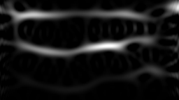
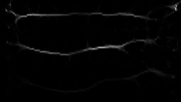
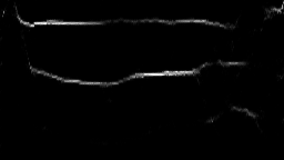
In order to test the effectiveness of the proposed method, a training set of 1320 signals and related SPWVD $P_{x}(t,f)$ and ideal TF distributions $I_{x}(t,f)$ were constructed using the TF toolbox [24]. We also used data augmentation to obtain input-output training pairs. The augmentation was done by first obtaining a smaller set and then applying various jittering operations. The time-domain signals have 256 samples. As a result the corresponding TF distributions are $256\times 256$ images. In addition, 120 test signals are generated for the validation purposes. The pix2pix network [10] was implemented using the Tensorflow Artificial Intelligence (AI) library [25]. The $\ell^{1}$ regularization parameter was set to $\lambda=100$ as selected by [10]. Similarly the Adam optimizer was selected with learning rate $\alpha=0.0002$, $\beta_{1}=0.5$ and $\beta_{2}=0.999$. The training was carried out for 50 epochs over the training set with batches of 10 images. In Figures 3, and 4 the result for two test signals are shown. Part (a) is the ideal TF representation of the signal $I_{x}(t,f)$ and (b) is the SPWVD $P_{x}(t,f)$. Part (c) shows the TF obtained by reassignment of SPWVD, namely RSPWVD. Part (d) is the proposed TF distribution obtained by pix2pix CGAN generator. Based on the Figures 3 and 4 it is clear that pix2pix CGAN produces high resolution TFs whose performance is comparable to the ideal TF. In order to asses the performance of the proposed CGAN based method a quantitative comparison is also carried out and the results are shown in Table I.

TABLE I: Performance comparison for SPVWD, RSPWVD and CGAN methods.

	Ideal TF			WVD			SPWVD			RSPWVD			CGAN TF
	pc $\uparrow$	$\ell^{1}\downarrow$	R $\downarrow$	pc $\uparrow$	$\ell^{1}\downarrow$	R $\downarrow$	pc $\uparrow$	$\ell^{1}\downarrow$	R $\downarrow$	pc $\uparrow$	$\ell^{1}\downarrow$	R $\downarrow$	pc $\uparrow$	$\ell^{1}\downarrow$	R $\downarrow$
$x_{1}$	1	0	9.82	0.27	1735	12.79	0.43	3606	12.88	0.52	820	10.80	0.49	753	10.32
$x_{2}$	1	0	9.64	0.46	816	10.82	0.57	1948	12.07	0.60	424	9.76	0.84	265	9.89
$x_{3}$	1	0	9.71	0.36	1067	11.66	0.56	1975	12.12	0.54	536	10.06	0.78	328	9.85
$x_{4}$	1	0	8.64	0.29	1036	12.52	0.34	1823	12.22	0.57	392	9.97	0.34	361	9.34
$x_{5}$	1	0	11.02	0.27	3757	13.87	0.49	5039	13.51	0.59	1524	11.37	0.67	1325	11.29
$x_{6}$	1	0	9.49	0.20	2052	12.80	0.44	2667	12.40	0.42	719	10.71	0.49	611	9.78
$x_{7}$	1	0	9.87	0.30	1570	12.58	0.48	3056	12.64	0.47	924	10.72	0.73	535	10.09
$x_{8}$	1	0	10.04	0.41	2379	12.80	0.55	3225	12.47	0.52	846	10.29	0.71	656	10.44
$x_{9}$	1	0	10.07	0.39	1927	13.06	0.45	4537	13.05	0.61	849	10.65	0.59	869	10.55
$x_{10}$	1	0	10.10	0.31	2381	13.21	0.52	3352	12.70	0.64	797	10.57	0.74	615	10.37
$\ldots$	$\ldots$	$\ldots$	$\ldots$	$\ldots$	$\ldots$	$\ldots$	$\ldots$	$\ldots$	$\ldots$	$\ldots$	$\ldots$	$\ldots$	$\ldots$	$\ldots$	$\ldots$
$Avg(120)$	1	0	9.82	0.33	1852	12.60	0.48	3075	12.58	0.55	771	10.48	0.64	610	10.16

The first 10 rows ($x_{1},x_{2},\ldots,x_{10}$) shows the result for 10 test signals. The bottom line is obtained by averaging the results for 120 test signals. Three metrics are considered. The first metric is the Pearson correlation (pc) [26] coefficient which is given by,

$$pc=\frac{P_{x}^{T}I_{x}}{\|P_{x}\|_{2}\|I_{x}\|_{2}}$$ (10)

where $P_{x}$ and $I_{x}$ are the vector form of related discrete TF matrices with the mean subtracted. Pearson correlation measures the shape similarity between the vectors. The higher the Pearson correlation the better the similarity. The arrow next to each metric indicates the desired direction. The second metric is the $\ell^{1}$ difference between the method and the ideal TF. The third measure is the Renyi entropy [27] which measures the TF localization. Renyi entropy is given by

$$R_{P}^{\alpha}=\frac{1}{1-\alpha}\log_{2}{\sum_{n=0}^{N}\sum_{m=0}^{M}P_{x}^{\alpha}[m,n]}.$$ (11)

where $\alpha$ is the order of Renyi. A Renyi entropy of order 3 was shown to be a good measure for localization [27]. The lower the Renyi measure the better the localization.

(a) Ideal TF

(b) SPWVD

(c) RSPWVD

(d) CGAN TF

Figure 3: Comparisson of TF distributions for a signal $x_{1}$ with three methods.

(a) Ideal TF

(b) SPWVD

(c) RSPWVD

(d) CGAN TF

Figure 4: Comparison of TF distributions for a signal $x_{2}$ with three methods.

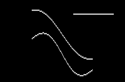
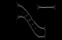
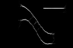
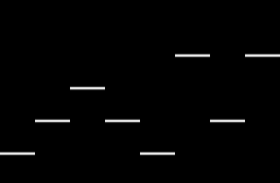
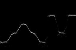
Table I clearly shows that the results obtained with the proposed CGAN approach are better than all the existing reassignment methods. For each metric the method performing the best is is printed in bold. Even though, the localization of RSPWVD and CGAN based method are comparable, CGAN based method is better in terms of $\ell^{1}$ measure and the Pearson correlation. This is attributed to the fact RSPWVD may have some $(t,f)$ points which do not express the underlying signal due to the nonlinear reassignment operation. Yet another comparison is made for a signal obtained from a Dolphin’s click-signal segment. The result is shown in Figure 5. Since it is not a synthetic signal the ideal TF is not known a priori, hence, is not shown. This figure also shows that the method successfully generates the TF representation.

(a) SPWVD

(b) RSPWVD

(c) CGAN TF

Figure 5: Comparison of TF distributions for a signal obtained from Dolphin’s click signal.

VI Conclusion

A method which generates high resolution TF representations was obtained using CGAN. The method uses SPWVD of the signal. Through examples it was shown that the performance is better than the existing methods, in particular the method gives better results than the reassignment method.

References

- [1] D. R. Wehner, High-Resolution Radar (2nd ed.). Boston: Artech House, 1994.
- [2] W. Y., L. H., and C. V. C., “ISAR motion compensation via adaptive joint time-frequency technique,” IEEE Transactions on Aerospace and Electronic Systems, vol. 34, no. 4, pp. 670–677, 1998.
- [3] K. Z. Thwe and N. War, “Environmental sound classification based on time-frequency representation,” in 2017 18th IEEE/ACIS International Conference on Software Engineering, Artificial Intelligence, Networking and Parallel/Distributed Computing (SNPD), 2017, pp. 251–255.
- [4] S. Chu, S. Narayanan, and C.-C. J. Kuo, “Environmental sound recognition with time–frequency audio features,” IEEE Transactions on Audio, Speech, and Language Processing, vol. 17, no. 6, pp. 1142–1158, 2009.
- [5] V. Mitra and H. Franco, “Time-frequency convolutional networks for robust speech recognition,” in 2015 IEEE Workshop on Automatic Speech Recognition and Understanding (ASRU), 2015, pp. 317–323.
- [6] T. A. C. M. Claasen and W. F. G. Mecklenbraiuker, “The Wigner distribution - A tool for time-frequency signal analysis; part III: relations with other time-frequency signal transformations,” Philips Journal of Research, vol. 35, no. 6, pp. 372 – 389, 1980.
- [7] F. Hlawatsch and G. Boudreaux-Bartels, “Linear and quadratic time-frequency signal representations,” IEEE Signal Process. Mag., vol. 9, no. 2, pp. 21–67, 1992.
- [8] P. Flandrin, F. Auger, and E. Chassande-Mottin, “Time-frequency reassignment: From principles to algorithms,” in A. Papandreou-Suppappola (Ed.), Applications in Time-Frequency Signal Processing. CRC Press, 2003, pp. 179 –203, ch. 5.
- [9] I. J. Goodfellow, J. Pouget-Abadie, M. Mirza, B. Xu, D. Warde-Farley, S. Ozair, A. Courville, and Y. Bengio, “Generative adversarial networks,” 2014.
- [10] P. Isola, J.-Y. Zhu, T. Zhou, and A. A. Efros, “Image-to-image translation with conditional adversarial networks,” 2018.
- [11] L. Cohen, “Time-frequency distributions - a review,” Proc. IEEE, vol. 77, no. 7, pp. 941–981, 1989.
- [12] D. L. Jones and R. G. Baraniuk, “An adaptive optimal-kernel time-frequency representation,” IEEE Trans. Signal Process., vol. 43, no. 10, pp. 2361 – 2371, 1995.
- [13] Z. Deprem and A. E. Çetin, “Crossterm-free Time-Frequency Distribution Reconstruction via Lifted Projections,” IEEE Transactions on Aerospace and Electronic Systems, vol. 51, no. 1, pp. 1–13, 2015.
- [14] Z. Deprem and A. E. Çetin, “Kernel estimation for time-frequency distribution,” in 2015 23nd Signal Processing and Communications Applications Conference (SIU), 2015, pp. 1973–1976.
- [15] Y. Lecun, L. Bottou, Y. Bengio, and P. Haffner, “Gradient-based learning applied to document recognition,” Proceedings of the IEEE, vol. 86, no. 11, pp. 2278–2324, 1998.
- [16] A. Buades, B. Coll, and J.-M. Morel, “A non-local algorithm for image denoising,” in 2005 IEEE Computer Society Conference on Computer Vision and Pattern Recognition (CVPR’05), vol. 2, 2005, pp. 60–65 vol. 2.
- [17] D. Eigen and R. Fergus, “Predicting depth, surface normals and semantic labels with a common multi-scale convolutional architecture,” 2015.
- [18] A. Radford, L. Metz, and S. Chintala, “Unsupervised representation learning with deep convolutional generative adversarial networks,” 2015, cite arxiv:1511.06434Comment: Under review as a conference paper at ICLR 2016. [Online]. Available: http://arxiv.org/abs/1511.06434
- [19] R. Zhang, P. Isola, and A. A. Efros, “Colorful image colorization,” 2016.
- [20] M. Mathieu, C. Couprie, and Y. LeCun, “Deep multi-scale video prediction beyond mean square error,” Jan. 2016, 4th International Conference on Learning Representations, ICLR 2016 ; Conference date: 02-05-2016 Through 04-05-2016.
- [21] X. Wang and A. Gupta, “Generative image modeling using style and structure adversarial networks,” 2016.
- [22] M. Mirza and S. Osindero, “Conditional generative adversarial nets,” 2014.
- [23] O. Ronneberger, P. Fischer, and T. Brox, “U-net: Convolutional networks for biomedical image segmentation,” 2015.
- [24] F. Auger, P. Flandrin, P. Gonçalves, and O. Lemoine, “Time-Frequency Toolbox For use with MATLAB,” 2005. [Online]. Available: http://tftb.nongnu.org
- [25] M. Abadi, P. Barham, J. Chen, Z. Chen, A. Davis, J. Dean, M. Devin, S. Ghemawat, G. Irving, M. Isard, M. Kudlur, J. Levenberg, R. Monga, S. Moore, D. G. Murray, B. Steiner, P. Tucker, V. Vasudevan, P. Warden, M. Wicke, Y. Yu, and X. Zheng, “Tensorflow: A system for large-scale machine learning,” in 12th USENIX Symposium on Operating Systems Design and Implementation (OSDI 16), 2016, pp. 265–283. [Online]. Available: https://www.usenix.org/system/files/conference/osdi16/osdi16-abadi.pdf
- [26] K. Pearson, “Notes on regression and inheritance in the case of two parents,” in Proceedings of the Royal Society of London, vol. 58, 1895, pp. 240–242.
- [27] R. G. Baraniuk, P. Flandrin, A. J. E. M. Janssen, and O. Michel, “Measuring time-frequency information content using the Rényi entropies,” IEEE Trans. Inf. Theory, vol. 47, no. 4, pp. 1391–1409, 2001.