Trees, forests, and total positivity:
I. $q$-trees and $q$-forests matrices

Abstract.

We consider matrices with entries that are polynomials in $q$ arising from natural $q$-generalisations of two well-known formulas that count: forests on $n$ vertices with $k$ components; and trees on $n+1$ vertices where $k$ children of the root are smaller than the root. We give a combinatorial interpretation of the corresponding statistic on forests and trees and show, via the construction of various planar networks and the Lindström-Gessel-Viennot lemma, that these matrices are coefficientwise totally positive. We also exhibit generalisations of the entries of these matrices to polynomials in eight indeterminates, and present some conjectures concerning the coefficientwise Hankel-total positivity of their row-generating polynomials.

1. Introduction

Two well-known enumerative formulas that often arise in the study of trees and forests are

$$f_{n}\coloneqq\;(n+1)^{n-1}$$ (1.1)

and

$$t_{n}\coloneqq\;(n+1)^{n}.$$ (1.2)

The first formula, $f_{n}$, gives the number of forests of rooted labelled trees on the vertex set $[n]:=\{1,2,\ldots,n\}$ and has the refinement:

$$f_{n}\;=\;\sum_{k=0}^{n}f_{n,k}$$ (1.3)

where each summand

$$f_{n,k}\coloneqq\binom{n-1}{k-1}n^{n-k}$$ (1.4)

is the number of forests on $[n]$ comprised of $k$ components (that is, $k$ rooted labelled trees). The first few $f_{n}$ and $f_{n,k}$ are

$$\begin{array}[]{c|rrrrrrr|r}\downarrow n,\rightarrow k&0&1&2&3&4&5&6&f_{n}\\ \hline\cr 0&1&&&&&&&1\\ 1&0&1&&&&&&1\\ 2&0&2&1&&&&&3\\ 3&0&9&6&1&&&&16\\ 4&0&64&48&12&1&&&125\\ 5&0&625&500&150&20&1&&1296\\ 6&0&7776&6480&2160&360&30&1&16807\end{array}$$ (1.5)

(see [63, A061356/A137452 and A000272]). By adding a new vertex (labelled $0$) and connecting it to the root of each component in a forest, we see that $f_{n}$ is also the number of trees on vertices labelled $0,1,\ldots,n$, rooted at $0$, where the root has precisely $k$ children.

The formula in (1.2), $t_{n}$, gives the number of rooted labelled trees on the vertex set $[n+1]$ and has the following refinement similar to (1.3):

$$t_{n}\;=\;\sum_{k=0}^{n}t_{n,k},$$ (1.6)

where each summand

$$t_{n,k}\coloneqq\binom{n}{k}n^{n-k}$$ (1.7)

is the number of rooted labelled trees on the vertex set $[n+1]$ in which precisely $k$ children of the root are lower-numbered than the root (see [7, 8, 65]). The first few $t_{n}$ and $t_{n,k}$ are:

$$\begin{array}[]{c|rrrrrrr|r}\downarrow n,\rightarrow k&0&1&2&3&4&5&6&t_{n}\\ \hline\cr 0&1&&&&&&&1\\ 1&1&1&&&&&&2\\ 2&4&4&1&&&&&9\\ 3&27&27&9&1&&&&64\\ 4&256&256&96&16&1&&&625\\ 5&3125&3125&1250&250&25&1&&7776\\ 6&46656&46656&19440&4320&540&36&1&117649\end{array}$$ (1.8)

(see [63, A071207]). We point out that this array has an alternative combinatorial interpretation; in [7, 8] the authors gave a bijection between trees on $n+1$ vertices where $k$ children of the root are lower-numbered than the root and forests on $n+1$ vertices with $k+1$ components where the vertex $n+1$ is a leaf.

The main goal of this paper is to prove the total positivity of some matrices that arise from generalisations of $f_{n,k}$ and $t_{n,k}$. Recall that a matrix is totally positive (strictly totally positive) if all of its minors are nonnegative (strictly positive, respectively). Total positivity has many applications across combinatorics, statistical physics, representation theory, and background material on the topic can be found in [42, 26, 51, 22].

Our first result concerns the forests (of rooted labelled trees) matrix

$$\mathsf{F}\coloneqq(f_{n,k})_{n,k\geq 0}\;=\;\left(\binom{n-1}{k-1}n^{n-k}\right)_{n,k\geq 0},$$ (1.9)

(the first few rows of which appear in (1.5)) and the (rooted labelled) trees matrix

$${\sf T}\coloneqq\left(t_{n,k}\right)_{n,k\geq 0}\;=\;\left(\binom{n}{k}n^{n-k}\right)_{n,k\geq 0},$$ (1.10)

(the first few entries of which appear in (1.8)). We have:

Theorem 1.1.

The matrices $\mathsf{F}$ and ${\sf T}$ are totally positive.

The total positivity of the forests and trees matrices has been proven very recently in [66, 67] using different methods to the ones we employ in the present paper. Sokal observes in [66] that $\mathsf{F}$ is the exponential Riordan array ${\mathcal{R}}[F,G]$ with $F(t):=1$ and $G(t)$ the tree function [16]

$$G(t)\coloneqq\sum_{n=1}^{\infty}n^{n-1}\frac{t^{n}}{n!},$$ (1.11)

and similarly in [67] Sokal and Chen observe that ${\sf T}$ is the exponential Riordan array ${\mathcal{R}}[F,G]$ with

$$F(t)\coloneqq\sum_{n=0}^{\infty}n^{n}\frac{t^{n}}{n!}\;=\;\frac{1}{1-G(t)}$$ (1.12)

and $G(t)$ as above. In [66] and [67] the author(s) exploit these intepretations of $\mathsf{F}$ and ${\sf T}$ and make use of the production-matrix method to prove these matrices are totally positive. The proof of Theorem 1.1 we offer below instead takes a leaf from [5, 24, 22], making use of the Lindström-Gessel-Viennot (LGV) lemma and planar networks (see Section 2.2).

The matrices $\mathsf{F}$ and ${\sf T}$ are closely related; by studying the entries one can, in effect, see the woods for the trees since for $n>0$

$$f_{n,k}\;=\;\binom{n-1}{k-1}n^{n-k}\;=\;\frac{k}{n}\binom{n}{k}n^{n-k}=\frac{k}{n}t_{n,k},$$ (1.13)

that is, $\mathsf{F}$ and ${\sf T}$ are related via a diagonal similarity transform (see Lemma 3.5 in Section 3.3):

$$\mathsf{F}\;=\;\lim_{\epsilon\to 0}\;\mathop{\rm diag}\nolimits((n+\epsilon)_{n\geq 0})^{-1}{\sf T}\mathop{\rm diag}\nolimits((k+\epsilon)_{k\geq 0})$$ (1.14)

where $\mathop{\rm diag}\nolimits({\mathbf{a}})$ denotes (for the sequence ${\mathbf{a}}=(a_{n})_{n\geq 0}$) the diagonal matrix with $(n,n)$-entry equal to $a_{n}$ and all other entries $0$ (note we must take a limit in the above to avoid division by zero in the first column of ${\sf T}$). Total positivity is preserved under matrix multiplication (this follows from the Cauchy-Binet formula), so (1.14) shows that the total positivity of ${\sf T}$ implies that of $\mathsf{F}$ (a diagonal matrix with nonnegative entries on the diagonal is clearly totally positive).

In fact there are a number of identities we present in Section 3.3 that allow one to go from ${\sf T}$ to $\mathsf{F}$ (and vice versa) via simple matrix multiplications that preserve total positivity. By specialising $q$ to $q=1$ in Lemma 3.11 below we obtain the identity

$${\sf T}\;=\;\mathsf{F}\cdot M$$ (1.15)

where $M\coloneqq(m_{n,k})_{n,k\geq 0}$ is the unit-lower-triangular matrix with $(n,k)$-entry

$$m_{n,k}\;=\;\frac{n!}{k!}$$ (1.16)

for $n\geq k$ and all other entries $0$. The matrix $M$ is easily shown to be totally positive (see Section 3.3), so it follows from (1.15) that the total positivity of $\mathsf{F}$ implies that of ${\sf T}$. In order to prove Theorem 1.1 it therefore suffices to prove that the forests matrix $\mathsf{F}$ is totally positive; we do this in Section 4 by constructing a planar network with nonnegative rational weights and showing that the corresponding path matrix is $\mathsf{F}$. The total positivity of $\mathsf{F}$ then follows from the LGV lemma (see Section 2.1).

In this paper, however, we are chiefly concerned with $q$-generalisations of the forests and trees matrices. The formula $f_{n,k}$ has a perfectly natural $q$-analogue, thus we define the $q$-forests matrix $\mathsf{F}(q)\coloneqq(f_{n,k}(q))_{n,k\geq 0}$ to be the matrix with $(n,k)$-entry

$$f_{n,k}(q)\coloneqq\begin{cases}\delta_{nk}&\textrm{if }k=0,\\ \displaystyle\genfrac{(}{)}{0.0pt}{}{n-1}{k-1}_{q}([n]_{q})^{n-k}&\textrm{if }n\geq k\geq 1,\\ 0&\textrm{otherwise.}\end{cases}$$ (1.17)

where

$$[n]_{q}\coloneqq\frac{1-q^{n}}{1-q}\;=\;\begin{cases}1+q+\cdots+q^{n-2}+q^{n-1}&\textrm{if }n>0,\\ 0&\textrm{if }n=0,\end{cases}$$ (1.18)

$\genfrac{(}{)}{0.0pt}{}{n}{k}_{q}$ is the $q$-binomial coefficient:

$$\genfrac{(}{)}{0.0pt}{}{n}{k}_{q}\coloneqq\frac{[n]_{q}!}{[k]_{q}![n-k]_{q}!},$$ (1.19)

in which

$$[n]_{q}!\coloneqq\begin{cases}\displaystyle\prod_{j=1}^{n}[j]_{q}&\textrm{if }n>0,\\ 1&\textrm{if }n=0,\end{cases}$$ (1.20)

and $\delta_{nk}$ is the Kronecker delta:

$$\delta_{nk}\coloneqq\begin{cases}1&\textrm{if }n=k,\\ 0&\textrm{if }n\neq k\end{cases}$$ (1.21)

It follows easily from (1.17) that $f_{n,k}(q)$ is a monic self-reciprocal polynomial of degree $(n-1)^{2}-(k-1)^{2}$, and the first few rows of $\mathsf{F}(q)$ are:

$$\left[\begin{array}[]{ccccc}1&&&&\\ 0&1&&&\\ 0&q+1&1&&\\ 0&q^{4}+2q^{3}+3q^{2}+2q+1&q^{3}+2q^{2}+2q+1&1&\\ \vdots&\vdots&\vdots&\vdots&\ddots\end{array}\right]$$ (1.22)

The $q$-forests matrix counts forests on $n$ vertices with $k$ components with respect to some statistic, which we interpret combinatorially in Section 3 (see Corollary 3.2). Please note that in [66] Sokal considers a different generalisation of $\mathsf{F}$ (he introduces indeterminates into $\mathsf{F}$ that count forests of rooted labelled trees in terms of proper and improper edges), whereas our results grew from studying natural $q$-generalisations of the matrix entries. In Section 6 we discuss how our generalisation gives rise to some curious conjectures concerning generalisations of well-known polynomial sequences including: the Schläfli-Gessel-Seo polynomials; the general Abel polynomials; $(p,q)$-Stirling cycle polynomials; and the reverse Bessel polynomials.

Each entry $t_{n,k}$ of the trees matrix has a similar natural $q$-analogue; we thus define the $q$-trees matrix to be ${\sf T}(q)\coloneqq(t_{n,k}(q))_{n,k\geq 0}$ where

$$t_{n,k}(q)\coloneqq\genfrac{(}{)}{0.0pt}{}{n}{k}_{q}([n]_{q})^{n-k}.$$ (1.23)

Once more it is easy to see that $t_{n,k}(q)$ is a monic self-reciprocal polynomial of degree $n(n-1)-k(k-1)$, and the first few rows of ${\sf T}(q)$ are:

$$\left[{\tiny\begin{array}[]{ccccc}1&&&&\\ 1&1&&&\\ q^{2}+2q+1&q^{2}+2q+1&1&&\\ q^{6}+3q^{5}+6q^{4}+7q^{3}+6q^{2}+3q+1&q^{6}+3q^{5}+6q^{4}+7q^{3}+6q^{2}+3q+1&q^{4}+2q^{3}+3q^{2}+2q+1&1&\\ \vdots&\vdots&\vdots&\vdots&\ddots\\ \end{array}}\right]$$ (1.24)

It follows from [7, 8] that the entries of the matrix ${\sf T}(q)$ count forests on $n+1$ vertices with $k+1$ components where the vertex $n+1$ is a leaf with respect to some statistic, and we give a combinatorial interpretation of $q$ in Section 3. We note that our $q$-generalisation of the tree matrix and the corresponding combinatorial interpretation differs from the generalisation of ${\sf T}$ studied by Chen and Sokal in [67].

The entries of $\mathsf{F}(q)$ and ${\sf T}(q)$ are polynomials in $q$ with integer coefficients, and there is a natural extension of total positivity to matrices whose entries are polynomials in one or more indeterminates ${\mathbf{x}}$. We equip the polynomial ring ${\mathbb{R}}[{\mathbf{x}}]$ with the coefficientwise partial order, that is, we say that $P$ is nonnegative (and write $P\succeq 0$) in case $P$ is a polynomial with nonnegative coefficients. We then say that a matrix with entries in ${\mathbb{R}}[{\mathbf{x}}]$ is coefficientwise totally positive (TP) if all of its minors are polynomials with nonnegative coefficients, and if all of its minors of size $\leq r$ are polynomials with nonnegative coefficients we say that the matrix is totally positive of order $r$ (TP_r). Our main result is the following:

Theorem 1.2.

The matrices $\mathsf{F}(q)$ and ${\sf T}(q)$ with entries in the polynomial ring ${\mathbb{Z}}[q]$ are coefficientwise totally positive.

It is plain to see that the above theorem reduces to Theorem 1.1 when $q$ is specialised to $q=1$. More generally, we say that a matrix $M$ with polynomial entries belonging to ${\mathbb{R}}[{\mathbf{x}}]$ is pointwise totally positive on some domain ${\mathcal{D}}\subseteq\mathbb{R}^{+}$ if $M$ is totally positive for all ${\mathbf{x}}\in{\mathcal{D}}$ (by which we mean all the indeterminates ${\mathbf{x}}$ are specialised to values in ${\mathcal{D}}$). Coefficientwise total positivity of $M$ thus implies pointwise total positivity for all ${\mathbf{x}}\in\mathbb{R}^{+}$, but the converse is not true.

The main goal of this paper is to prove Theorem 1.2 and the structure of our proof is as follows: after reviewing some basic concepts in total positivity from the perspective of planar networks in Section 2, we then provide combinatorial interpretations of the entries of $\mathsf{F}(q)$ and ${\sf T}(q)$ in Section 3 and establish some identities that show the coefficientwise total positivity of $\mathsf{F}(q)$ implies that of ${\sf T}(q)$. In Section 4 we construct a planar network with weights that are rational and pointwise nonnegative functions of $q$, and prove that the path matrix corresponding to this planar network agrees with $\mathsf{F}(q)$; thanks to the LGV lemma this proves pointwise total positivity of $\mathsf{F}(q)$ and ${\sf T}(q)$ for $q\in\mathbb{R}^{+}$ (Theorem 1.1 is then obtained by specialising $q$ to $q=1$). In Section 5 we show how the network from Section 4 can be transformed into a planar network with weights that are polynomials in $q$, thereby proving Theorem 1.2. We conclude in Section 6 with some further generalisations and open problems, some of which will be the subject of future work.

2. Preliminaries

Here we review some fundamental definitions and facts regarding total positivity. Please note that since our proofs rely on Lindström-Gessel-Viennot lemma, many of the results in this section are motivated by performing operations on planar networks (see [22, 24, 5, 6]), from which various matrix identites follow.

2.1. Total positivity and the Lindström-Gessel-Viennot lemma

One fundamental tool in the study of total positivity is the Lindström-Gessel-Viennot (LGV) lemma. Suppose $G$ is a locally finite acyclic digraph with source vertices $U\coloneqq\{u_{0},u_{1},\ldots,u_{n}\}$ and sink vertices $V\coloneqq\{v_{0},v_{1},\ldots,v_{n}\}$, where the weight $w_{e}$ of an edge $e$ is an element of some commutative ring $R$. Let $w(P(u_{i},v_{j}))$ denote the product of the weights of the edges of a path $P(u_{i},v_{j})$ starting at $u_{i}$ and ending at $v_{j}$, and define

$$P_{G}(u_{i}\to v_{j})\coloneqq\sum_{P(u_{i},v_{j})}w(P(u_{i},v_{j}))$$ (2.1)

to be the sum over all weighted paths between $u_{i}$ and $v_{j}$. The path matrix corresponding to $G$ is then the matrix

$$P_{G}\coloneqq(P_{G}(u_{i}\to v_{j}))_{0\leq i,j\leq n}.$$ (2.2)

We say that a family of nonintersecting paths from $U$ to $V$ is an $n$-tuple $(P_{0},P_{1},\ldots,P_{n})$ of paths in $G$ such that:

1. There exists a permutation $\sigma$ of $\{0,1,2,\ldots,n\}$ such that for each $i$, $P_{i}$ is a path from $u_{i}$ to $v_{\sigma(i)}$.

2. Whenever $i\neq j$, paths $P_{i}$ and $P_{j}$ have no vertices in common (this includes endpoints).

The LGV lemma states that

$$\det(P_{G})\;=\;\sum_{(P_{0},P_{1},\ldots,P_{n}):U\to V}\mathop{\rm sgn}\nolimits(\sigma)\prod_{i=0}^{n}w(P_{i}),$$ (2.3)

where $\mathop{\rm sgn}\nolimits(\sigma)=(-1)^{{\rm inv}(\sigma)}$ is the signature of the permutation $\sigma$ arising from $P_{i}$ mapping $u_{i}$ to $v_{\sigma(i)}$ (note that ${\rm inv}(\sigma)$ denotes the number of inversions of $\sigma$, that is, pairs $(i,j)$ in $\{0,1,\ldots,n\}$ such that $i<j$ and $\sigma(i)>\sigma(j)$). In particular, if the only permutation giving rise to nonempty families of nonintersecting paths is the identity then $\det(P_{G})$ gives the sum over all weighted families of nonintersecting paths in $G$ that begin at $U$ and end at $V$, where the weight of each family is the product of the weights of the paths $(P_{0},\ldots,P_{n})$.

Suppose now the source and sink vertices of $G$ are fully compatible, by which we mean that for any subset of sources $u_{n_{1}},u_{n_{2}},\ldots,u_{n_{r}}$ (where $n_{1}<n_{2}<\cdots<n_{r}$) and sinks $v_{k_{1}},v_{k_{2}},\ldots,v_{k_{r}}$ (where $k_{1}<k_{2}<\ldots<k_{r}$), the only permutation $\sigma\in\mathfrak{S}_{r}$ mapping each source $u_{n_{i}}$ to the sink $v_{k_{\sigma(i)}}$ that gives rises to nonempty families of paths is the identity. The LGV lemma then implies that every minor of $P_{G}$ is a sum over families of nonintersecting paths between specified subsets of $U$ and $V$, where each family has weight $\prod w(P_{i})$. If every edge has a weight that is a positive real number then $P_{G}$ is totally positive; if the weights of the network belong to the field ${\mathbb{Q}}({\mathbf{x}})$ of rational functions of ${\mathbf{x}}$ that are pointwise nonnegative on some domain ${\mathcal{D}}$ then $P_{G}$ is pointwise totally positive on ${\mathcal{D}}$; and if the weight of each edge is a polynomial in the indeterminates ${\mathbf{x}}$ with nonnegative integer coefficients then $P_{G}$ is totally positive in ${\mathbb{Z}}[{\mathbf{x}}]$ equipped with the coefficientwise order.

Determining whether a general locally finite acyclic digraph is fully compatible is non-trivial, however, if $G$ is embedded in the plane and the source and sink vertices $U$ and $V$ lie on the boundary of $G$ in the order “first $U$ in reverse order, then $V$ in order” then the topology of $G$ clearly implies that $U$ and $V$ are fully compatible (see, for example, Lemma 9.18 in [49]). From now on we will refer to locally acyclic digraphs embedded in the plane with fully compatible sources and sinks as planar networks, in the spirit of [24].

2.2. The binomial-like planar network

Figure 1. The binomial-like planar network ${\mathcal{N}}$ for vertices $u_{0},u_{1},\ldots,u_{5}$ and $v_{0},v_{1},\ldots,v_{5}$.

The matrices ${\sf T}(q)$ and $\mathsf{F}(q)$ are unit-lower-triangular, so in the sequel we will be principally concerned with what we call the binomial-like planar network (depicted in Figure 1). This planar network consists of vertices indexed by $i$ ($j$) increasing horizontally from the right (vertically upwards, respectively) where $0\leq i\leq j$. Each source $u_{i}$ is the vertex with index $(i,i)$ while each sink $v_{j}$ is the vertex $(0,j)$. Each horizontal edge directed from vertex $(i,j)$ to vertex $(i-1,j)$ has weight $\alpha_{i,j-i+1}$, while the weight of a diagonal edge directed from vertex $(i,j)$ to $(i-1,j-1)$ has weight $\beta_{i,j-i}$. We also assume there exists a directed edge from $u_{0}$ to $v_{0}$ with weight 1.

The binomial-like planar network with weights $\boldsymbol{\alpha}=\{\alpha_{i,l}\}_{i,l\geq 1}$ and $\boldsymbol{\beta}=\{\beta_{i,l}\}_{i\geq 1,l\geq 0}$ described above is denoted ${\mathcal{N}}$. Please note that the source and sink vertices of ${\mathcal{N}}$ are fully compatible, so it follows immediately from the LGV lemma that the path matrix $P_{{\mathcal{N}}}$ is automatically coefficientwise totally positive over ${\mathbb{Z}}[\boldsymbol{\alpha},\boldsymbol{\beta}]$ in all of these indeterminates!

This is really the beauty of the LGV lemma (in the context of total positivity): given a lower-triangular matrix $M$ that appears to be coefficientwise totally positive in ${\mathbb{R}}[{\mathbf{x}}]$, one can try to prove total positivity by specialising $\alpha_{i,l}$, $\beta_{i,l}$ to suitable nonnegative elements of ${\mathbb{R}}[{\mathbf{x}}]$ and showing that under such a specialisation

$$P_{{\mathcal{N}}}\;=\;M.$$ (2.4)

Indeed, this is how we concoct our proof of Theorem 1.2. We first show that specialising the weights of the binomial-like network to suitably chosen rational functions of $q$ yields a path matrix that agrees with $\mathsf{F}(q)$ in Section 4; since these rational functions are all nonnegative for $q\in\mathbb{R}^{+}$ we conclude that $\mathsf{F}(q)$ is pointwise totally positive for $q\in\mathbb{R}^{+}$. In Section 5 we then transform this binomial-like network to obtain a different planar network with weights that are polynomials in $q$ in order to show that $\mathsf{F}(q)$ is coefficientwise totally positive.

The planar network construction described above originally goes back to Brenti [5] who also observed that if the binomial-like network ${\mathcal{N}}$ has weights $\boldsymbol{\alpha}$ and $\boldsymbol{\beta}$ that depend purely on the first index (that is, $\alpha_{i,l}=\alpha_{i,*}$ and $\beta_{i,l}=\beta_{i,*}$ for all $i$) then the entries of the path matrix $P_{{\mathcal{N}}}$ satisfy the $n$-dependent recurrence

$$P_{{\mathcal{N}}}(u_{n}\to v_{k})\;=\;\alpha_{n,*}\,P_{{\mathcal{N}}}(u_{n-1}\to v_{k-1})\>+\>\beta_{n,*}\,P_{{\mathcal{N}}}(u_{n-1}\to v_{k})\;.$$ (2.5)

Similarly if the weights depend solely on the second index (that is, $\alpha_{i,l}=\alpha_{*,l}$ and $\beta_{i,l}=\beta_{*,l}$ for all $l$) then the entries of the path matrix satisfy the $k$-dependent recurrence

$$P_{{\mathcal{N}}}(u_{n}\to v_{k})\;=\;\alpha_{*,k}\,P_{{\mathcal{N}}}(u_{n-1}\to v_{k-1})\>+\>\beta_{*,k}\,P_{{\mathcal{N}}}(u_{n-1}\to v_{k})\;.$$ (2.6)

The most straightforward (and thus, eponymous) example that illustrates this connection between matrices with entries satisfying purely $n$- (or $k$-) dependent recurrences and binomial-like planar networks is the weighted binomial matrix,

$$B_{x,y}\coloneqq\left(\binom{n}{k}x^{n-k}y^{k}\right)_{n,k\geq 0},$$ (2.7)

the entries of which satisfy the $n$-dependent linear recurrence

$$(B_{x,y})_{n,k}\;=\;x(B_{x,y})_{n-1,k}+y(B_{x,y})_{n-1,k-1}$$ (2.8)

for $n>0$ with initial condition $(B_{x,y})_{0,k}=\delta_{0k}$. The corresponding planar network is the network ${\mathcal{N}}$ with $\alpha_{i,l}=y$ and $\beta_{i,l}=x$, and it follows immediately from the LGV lemma that

Corollary 2.1.

The weighted binomial matrix $B_{x,y}$ is coefficientwise totally positive in ${\mathbb{Z}}[x,y]$.

Matrices with entries given by purely $n$-dependent or purely $k$-dependent recurrences have relatively straightforward planar network representations, and often in these cases it is easy to deduce a straightforward planar network by studying the recurrence.

Matrices with entries that satisfy recurrences dependent on both $n$ and $k$, however, give rise to seemingly much more complex planar networks (see, for example, [11]). For example, the entries of the forests matrix

$$\mathsf{F}\;=\;(f_{n,k})_{n,k\geq 0}\;=\;\left(\binom{n-1}{k-1}n^{n-k}\right)_{n,k\geq 0},$$ (2.9)

satisfy the recurrence:

$$f_{n,k}\;=\;\left(\frac{n}{n-1}\right)^{n-1}\left[(n-1)f_{n-1,k}+\frac{1}{k-1}\left(n\left(\frac{n-1}{n}\right)^{k}+(k-n)\right)f_{n-1,k-1}\right]$$ (2.10)

for $n>1$  with initial conditions $f_{n,0}=\delta_{n0}$, and $f_{1,1}=1$. We note that we were able to find the correct weights for the binomial-like planar network corresponding to $\mathsf{F}$ in spite of this complicated recurrence, and not because of it.

In the sequel we will also make use of the following fact. Suppose $\alpha_{i,l}=1$ and consider the sum over all weighted paths from $u_{n}$ to $v_{k}$ in ${\mathcal{N}}$ (denoted $P_{{\mathcal{N}}}(u_{n}\to v_{k})$). By studying the network it is relatively easy to see that $P_{{\mathcal{N}}}(u_{n}\to v_{k})$ can be expressed as a nested sum

$$P_{{\mathcal{N}}}(u_{n}\to v_{k}) = \sum_{i_{1}=1}^{k+1}\beta_{i_{1},k+1-i_{1}}\sum_{i_{2}=i_{1}+1}^{k+2}\beta_{i_{2},k+2-i_{2}}\cdots\sum_{i_{n-k}=i_{n-k-1}+1}^{n}\beta_{i_{n-k},n-i_{n-k}}$$ (2.11)

$$= \sum_{1\leq i_{1}<\cdots<i_{n-k}\leq n}\beta_{i_{1},k+1-i_{1}}\beta_{i_{2},k+2-i_{2}}\cdots\beta_{i_{n-k},n-i_{n-k}}.$$ (2.12)

Observe that if the weights $\beta_{i,l}$ are dependent only on the first index then $P_{{\mathcal{N}}}(u_{n}\to v_{k})$ can be realised as the elementary symmetric polynomial

$${\mathbf{e}}_{n-k}(X_{1},X_{2},\ldots,X_{n})\coloneqq\sum_{1\leq i_{1}<\cdots<i_{n-k}\leq n}X_{i_{1}}X_{i_{2}}\cdots X_{i_{n-k}}$$ (2.13)

where $X_{n}\coloneqq\beta_{n,*}$. If instead the weights $\beta_{i,l}$ depend solely on the second index then (2.12) can be realised as the complete homogeneous symmetric polynomial

$${\mathbf{h}}_{n-k}(X_{1},X_{2},\ldots,X_{k+1})\coloneqq\sum_{1\leq i_{1}\leq\cdots\leq i_{n-k}\leq k+1}X_{i_{1}}X_{i_{2}}\cdots X_{i_{n-k}}$$ (2.14)

where $X_{k}=\beta_{*,k-1}$ (this observation again goes back to Brenti [5]).

In this article we study total positivity primarily through the lens of planar networks; the next section dicusses how planar networks can be intepreted algebraically as matrix factorisations.

2.3. Matrix factorisations

The planar network approach outlined above allows us to easily write down various factorisations of the path matrix $P_{{\mathcal{N}}}$. Before discussing these factorisations we first clarify some notation. We use ${\mathcal{N}}$ to denote the binomial-like network described in the previous subsection with the set of horizontal weights $\boldsymbol{\alpha}$ and diagonal weights $\boldsymbol{\beta}$. Conversely, given a matrix $M$, in this section we will often use ${\mathcal{N}}_{M}$ to denote a planar network with corresponding path matrix $P_{{\mathcal{N}}_{M}}$ satisfying

$$P_{{\mathcal{N}}_{M}}\;=\;M.$$ (2.15)

In this case ${\mathcal{N}}_{M}$ is referred to as a planar network representation of the matrix $M$.

We will make much use of the following definition. For sequences ${\mathbf{a}}\coloneqq(a_{n})_{n\geq 0}$ and ${\mathbf{b}}\coloneqq(b_{n})_{n\geq 0}$, let $L({\mathbf{a}},{\mathbf{b}})$ denote the lower-bidiagonal matrix with $(n,k)$-entry

$$\left(L({\mathbf{a}},{\mathbf{b}})\right)_{n,k\geq 0}\;=\;\begin{cases}a_{k}&\textrm{if }n=k,\\ b_{k}&\textrm{if }n=k+1,\\ 0&\textrm{otherwise.}\end{cases}$$ (2.16)

The first few rows and columns of $L({\mathbf{a}},{\mathbf{b}})$ are:

$$L({\mathbf{a}},{\mathbf{b}})\;=\;\left[\begin{array}[]{cccccccc}a_{0}&&&&&&&\\ b_{0}&a_{1}&&&&&&\\ &b_{1}&a_{2}&&&&&\\ &&b_{2}&a_{3}&&&&\\ &&&b_{3}&a_{4}&&&\\ &&&&b_{4}&a_{5}&&\\ &&&&&b_{5}&a_{6}&\\ &&&&&&\ddots&\ddots\end{array}\right].$$ (2.17)

In case $a_{n}=1$ for all $n$ we abbreviate $L({\mathbf{a}},{\mathbf{b}})$ to $L({\mathbf{b}})$, while if $b_{n}=0$ for all $n$ the matrix $L({\mathbf{a}},{\mathbf{b}})$ is simply the diagonal matrix $\mathop{\rm diag}\nolimits({\mathbf{a}})$ with $(n,n)$-entry $a_{n}$ and all other entries $0$. Lastly, if $a_{n}=1$ and the sequence ${\mathbf{b}}$ is constant, that is, $b_{n}=x$ for all $n$, we abbreviate $L({\mathbf{b}})$ to $L(x)$, and if we have $a_{n}=x$ and $b_{n}=y$ for all $n$ with $y\neq 1$ we abbreviate $L({\mathbf{a}},{\mathbf{b}})$ to $L(x,y)$.

The lower-bidiagonal matrix $L({\mathbf{a}},{\mathbf{b}})$ has a planar network representation ${\mathcal{N}}_{L({\mathbf{a}},{\mathbf{b}})}$ in which

$$P_{{\mathcal{N}}_{L({\mathbf{a}},{\mathbf{b}})}}(u_{n}\to v_{n})\;=\;a_{n}$$ (2.18)

and

$$P_{{\mathcal{N}}_{L({\mathbf{a}},{\mathbf{b}})}}(u_{n}\to v_{n-1})\;=\;b_{n-1}$$ (2.19)

(see the diagram on the left in Figure 2). Since we view these matrices through the lens of planar networks we will refer to the sequences ${\mathbf{a}}$ and ${\mathbf{b}}$ as edge-sequences corresponding to $L({\mathbf{a}},{\mathbf{b}})$. According to the LGV lemma we have:

Figure 2. The planar network ${\mathcal{N}}_{L({\mathbf{a}},{\mathbf{b}})}$ (left), and the planar network that arises from expressing $L({\mathbf{a}},{\mathbf{b}})$ as a product of elementary lower-bidiagonal transfer matrices and concatenating the networks $N_{E_{0}(a_{0},b_{0})},N_{E_{1}(a_{1},b_{1})},\dots$ (right). Note that unlabelled directed edges are assumed to have weight 1.

Corollary 2.2 (Lower-bidiagonal matrices).

The matrix $L({\mathbf{a}},{\mathbf{b}})$ is totally positive in ${\mathbb{Z}}[{\mathbf{a}},{\mathbf{b}}]$ equipped with the coefficientwise order.

It is straightforward to verify that

$$L({\mathbf{a}},{\mathbf{b}})\;=\;E_{0}(a_{0},b_{0})E_{1}(a_{1},b_{1})E_{2}(a_{2},b_{2})\cdots$$ (2.20)

where $E_{n}(a,b)$ denotes the elementary (lower) bidiagonal matrix with $(n,n)$-entry $a$, $(n+1,n)$-entry $b$, all other diagonal entries 1, and all other entries $0$. As with bidiagonal matrices, in case $a=1$ we abbreviate $E_{n}(1,b)$ to $E_{n}(b)$. We now present a useful lemma relating matrix products and concatenated planar networks:

Lemma 2.3 (Concatenating planar networks).

Suppose $M_{1}$ and $M_{2}$ are path matrices corresponding to two planar networks ${\mathcal{N}}_{M_{1}}$ and ${\mathcal{N}}_{M_{2}}$, where ${\mathcal{N}}_{M_{1}}$ has source vertices

$$U\coloneqq\{u_{0},u_{1},\ldots,u_{n}\}$$ (2.21)

and sink vertices

$$V\coloneqq\{v_{0},v_{1},\ldots,v_{m}\},$$ (2.22)

and ${\mathcal{N}}_{M_{2}}$ has source vertices

$$U^{\prime}\coloneqq\{u^{\prime}_{0},u^{\prime}_{1},\ldots,u^{\prime}_{m}\}$$ (2.23)

and sink vertices

$$V^{\prime}=\{v^{\prime}_{0},v^{\prime}_{1},\ldots,v^{\prime}_{l}\}.$$ (2.24)

Then the matrix product $M_{1}M_{2}$ is the path matrix corresponding to the planar network ${\mathcal{N}}_{M_{3}}$ obtained by concatenating $M_{1}$ and $M_{2}$, with source vertices $U$ and sink vertices $V^{\prime}$, where each vertex $v_{i}\in V$ is identified with $u^{\prime}_{i}\in U^{\prime}$ for all $i$.

Proof.

Since $v_{i}$ is identified with $u^{\prime}_{i}$ we can write the sum over over weighted paths from $u_{n}$ to $v^{\prime}_{k}$ in ${\mathcal{N}}_{M_{3}}$ as

$$P_{{\mathcal{N}}_{M_{3}}}(u_{n}\to v^{\prime}_{k})=\sum_{s=0}^{m}P_{{\mathcal{N}}_{M_{1}}}(u_{n}\to v_{s})P_{{\mathcal{N}}_{M_{2}}}(u^{\prime}_{s}\to v_{k}^{\prime})\;=\;(M_{1}M_{2})_{n,k}.$$ (2.25)

∎

Concatenating planar networks thus corresponds to multiplying path matrices, and the matrices $M_{1}$ and $M_{2}$ in the above are referred to as transfer matrices of the planar network ${\mathcal{N}}_{M_{3}}$. The elementary bidiagonal matrices on the right-hand side of (2.20) are thus transfer matrices of ${\mathcal{N}}_{L({\mathbf{a}},{\mathbf{b}})}$, and concatenating the planar networks for $E_{0}(a_{0},b_{0}),E_{1}(a_{1},b_{1}),\ldots$ yields the planar network on the right in Figure 2.

Figure 3. The planar network ${\mathcal{N}}_{1}$ up to sources $u_{0},u_{1},\ldots,u_{4}$ and $v_{0},v_{1},\ldots,v_{4}$ (unlabelled directed edges have weight $1$).

We now interpret the binomial-like planar network ${\mathcal{N}}$ and its path matrix $P_{{\mathcal{N}}}$ from Subsection 2.2 in light of these definitions. By extending the source vertices of ${\mathcal{N}}$ to the left so that they lie on the same vertical line we obtain a planar network ${\mathcal{N}}_{1}$ that is isomorphic to ${\mathcal{N}}$ (see Figure 3), in particular we have

$$P_{{\mathcal{N}}}(u_{n}\to v_{k})\;=\;P_{{\mathcal{N}}_{1}}(u_{n}\to v_{k}).$$ (2.26)

Consider a subnetwork $C^{i}$ of ${\mathcal{N}}_{1}$ consisting of source vertices $U\coloneqq\{(i+1,j):j\in{\mathbb{N}}\}$ and sink vertices $V\coloneqq\{(i,j):j\in{\mathbb{N}}\}$. Let ${\mathbf{a}}_{i}$ denote the sequence of weights of horizontally directed edges emanating from vertex $(i+1,i+n)$ for increasing $n$, that is, ${\mathbf{a}}_{i}\coloneqq(a_{n})_{n\geq 0}$ where

$$a_{n}\;=\;\begin{cases}\alpha_{i+1,n}&\textrm{if }n>0,\\ 1&\textrm{if }n=0\end{cases}.$$ (2.27)

Similarly let ${\mathbf{b}}_{i}$ denote the sequence of weights of the diagonal edges emanating from vertex $(i+1,i+n+1)$ for increasing $n$, that is, ${\mathbf{b}}_{i}\coloneqq(\beta_{i+1,n})_{n\geq 0}$. It is easy to see that the path matrix corresponding to $C^{i}$ is the column transfer matrix

$$P_{C^{i}}\;=\;\left[\begin{array}[]{c|c}I_{i}&0\\ \hline\cr 0&L({\mathbf{a}}_{i},{\mathbf{b}}_{i})\end{array}\right]$$ (2.28)

where $I_{i}$ is the identity matrix of size $i$, and $L({\mathbf{a}}_{i},{\mathbf{b}}_{i})$ is the lower-bidiagonal matrix with corresponding edge sequences ${\mathbf{a}}_{i}$ and ${\mathbf{b}}_{i}$. Obviously the matrix $P_{C^{i}}$ is totally positive in ${\mathbb{Z}}[{\mathbf{a}},{\mathbf{b}}]$ equipped with the coefficientwise order.

Since ${\mathcal{N}}_{1}$ is the concatenation of column transfer matrices we immediately obtain what we refer to as a production-like factorisation of $P_{{\mathcal{N}}}$:

Corollary 2.4 (Production-like factorisation).

The path matrix $P_{{\mathcal{N}}}$ corresponding to the binomial-like planar network ${\mathcal{N}}$ has the factorisation:

$$P_{{\mathcal{N}}}\;=\;\cdots\left[\begin{array}[]{c|c}I_{2}&0\\ \hline\cr 0&L({\mathbf{a}}_{2},{\mathbf{b}}_{2})\end{array}\right]\cdot\left[\begin{array}[]{c|c}I_{1}&0\\ \hline\cr 0&L({\mathbf{a}}_{1},{\mathbf{b}}_{1})\end{array}\right]\cdot L({\mathbf{a}}_{0},{\mathbf{b}}_{0})$$ (2.29)

where ${\mathbf{a}}_{i}=(\alpha_{i+1,n})_{n\geq 0}$ (with $\alpha_{i+1,0}=1$) and ${\mathbf{b}}_{i}=(\beta_{i+1,n})_{n\geq 0}$.

Recall from the previous subsection that the weighted binomial matrix $B_{x,y}$ is the path matrix of the binomial-like network ${\mathcal{N}}$ with $\alpha_{i,l}=y$ and $\beta_{i,l}=x$. The above corollary thus yields the following factorisation of $B_{x,y}$:

Corollary 2.5 (Production-like factorsation of $B_{x,y}$).

The matrix $B_{x,y}$ has the production-like factorisation

$$B_{x,y}\;=\;\cdots\left[\begin{array}[]{c|c}I_{2}&0\\ \hline\cr 0&L({\bf y},x)\end{array}\right]\cdot\left[\begin{array}[]{c|c}I_{1}&0\\ \hline\cr 0&L({\bf y},x)\end{array}\right]\cdot L({\bf y},x)$$ (2.30)

where $L({\bf y},x)$ denotes the lower-bidiagonal matrix with $(0,0)$-entry 1, all other diagonal entries $y$, all subdiagonal entries $x$, and all other entries $0$.

We note that the above corollary imples that $B_{x,y}$ satisfies

$$B_{x,y}\;=\;\left[\begin{array}[]{c|c}1&0\\ \hline\cr 0&B_{x,y}\end{array}\right]L({\bf y},x).$$ (2.31)

Figure 4. The planar network ${\mathcal{N}}_{T({\mathbf{a}})}$ that has corresponding path matrix $T({\mathbf{a}})$.

There are other ways to factorise $P_{{\mathcal{N}}}$ that rely on the following helpful definition. Given a sequence ${\mathbf{a}}=(a_{n})_{n\geq 0}$ let $T({\mathbf{a}})\coloneqq(a^{*}_{n,k})_{n,k\geq 0}$ denote the lower-triangular matrix with $(n,k)$-entry

$$a^{*}_{n,k}\;=\;\prod_{j=k}^{n-1}a_{j}$$ (2.32)

for $n\geq k$ and 0 in all other cases (we consider the empty product arising from $n=k$ to be $1$). The first few rows and columns of $T({\mathbf{a}})$ are thus:

$$T({\mathbf{a}})\;=\;\left[\begin{array}[]{ccccccc}1&&&&&&\\ a^{*}_{1,0}&1&&&&&\\ a^{*}_{2,0}&a^{*}_{2,1}&1&&&&\\ a^{*}_{3,0}&a^{*}_{3,1}&a^{*}_{3,2}&1&&&\\ a^{*}_{4,0}&a^{*}_{4,1}&a^{*}_{4,2}&a^{*}_{4,3}&1&&\\ a^{*}_{5,0}&a^{*}_{5,1}&a^{*}_{5,2}&a^{*}_{5,3}&a^{*}_{5,4}&1&\\ \vdots&\vdots&\vdots&\vdots&\vdots&\vdots&\ddots\\ \end{array}\right].$$ (2.33)

The matrix $T({\mathbf{a}})$ is the path matrix corresponding to the planar network ${\mathcal{N}}_{T({\mathbf{a}})}$ in which

$$P_{{\mathcal{N}}_{T({\mathbf{a}})}}(u_{n}\to v_{k})\;=\;a^{*}_{n,k}$$ (2.34)

(see Figure 4). Clearly $T({\mathbf{a}})$ is totally positive in ${\mathbb{Z}}[{\mathbf{a}}]$ equipped with the coefficientwise order, and by comparing Figure 2 with Figure 4 and (2.20) it is easy to see that

$$T({\mathbf{a}})\;=\;\cdots E_{2}(a_{2})E_{1}(a_{1})E_{0}(a_{0})=(E_{0}(-a_{0})^{-1}E_{1}(-a_{1})^{-1}E_{2}(-a_{2})^{-1}\cdots)^{-1},$$ (2.35)

since $E_{n}(a)^{-1}=E_{n}(-a)$. We thus obtain the following corollary:

Corollary 2.6 (Inverse lower-bidiagonal matrices).

For a sequence ${\mathbf{a}}=(a_{n})_{n\geq 0}$ we have

$$T({\mathbf{a}})\;=\;L(-{\mathbf{a}})^{-1}$$ (2.36)

where $-{\mathbf{a}}=(-a_{n})_{n\geq 0}$.

In light of Corollary 2.6 we refer to the matrix $T({\mathbf{a}})$ as an inverse (lower-)bidiagonal matrix with corresponding edge sequence ${\mathbf{a}}$. The case where $a_{n}=x$ for all $n$ often arises in the study of total positivity, and $T({\mathbf{a}})$ is then referred to as a Toeplitz matrix of powers of $x$ since each $(n,k)$ entry is $x^{n-k}$, and we denote it $T_{\infty}(x)$. It follows from the LGV lemma that $T_{\infty}(x)$ is coefficientwise totally positive in ${\mathbb{Z}}[x]$. More generally, given a sequence ${\mathbf{a}}=(a_{n})_{n\geq 0}$ we call the infinite lower-triangular matrix $T_{\infty}({\mathbf{a}})=(a_{n-k})_{n,k\geq 0}$ where $a_{l}=0$ for $l<0$ the (infinite) Toeplitz matrix associated to ${\mathbf{a}}$.

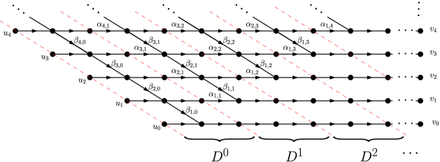
Figure 5. The planar network ${\mathcal{N}}_{2}$ up to source $u_{4}$ and sink $v_{4}$ (unlabelled edges have weight 1). Please note the red dashed lines are not part of the planar network, they delineate the sources and sinks of each diagonal transfer matrix $D^{l}$.

Let us return again to the binomial-like planar network ${\mathcal{N}}$. Observe that ${\mathcal{N}}$ is isomorphic to the planar network ${\mathcal{N}}_{2}$ in Figure 5, in particular we have

$$P_{{\mathcal{N}}}(u_{n}\to v_{k})\;=\;P_{{\mathcal{N}}_{2}}(u_{n}\to v_{k})$$ (2.37)

for all $n,k\geq 0$.

Consider a subnetwork $D^{l}$ of ${\mathcal{N}}_{2}$ contained between a pair of consecutive dashed diagonal lines. The path matrix for each such subnetwork is the diagonal transfer matrix:

$$P_{D^{l}}\;=\;\left[\begin{array}[]{c|c}I_{l}&0\\ \hline\cr 0&\mathop{\rm diag}\nolimits({\mathbf{a}}_{l})T({\mathbf{b}}_{l})\end{array}\right]$$ (2.38)

where ${\mathbf{a}}_{0}=(1)_{n\geq 0}$, ${\mathbf{a}}_{l}=(\alpha_{n+1,l})_{n\geq 0}$ for $l>0$, and ${\mathbf{b}}_{l}=(\beta_{n+1,l})_{n\geq 0}$ for all $l$.

The concatenation of subnetworks $D^{0},D^{1},\ldots$ from left to right yields a different factorisation of $P_{{\mathcal{N}}},$ namely its quasi-production-like factorisation:

Corollary 2.7 (Quasi-production-like factorisation).

The path matrix $P_{{\mathcal{N}}}$ has the factorisation

$$P_{{\mathcal{N}}}\;=\;T({\mathbf{b}}_{0})\cdot\left[\begin{array}[]{c|c}I_{1}&0\\ \hline\cr 0&\mathop{\rm diag}\nolimits({\mathbf{a}}_{1})T({\mathbf{b}}_{1})\end{array}\right]\cdot\left[\begin{array}[]{c|c}I_{2}&0\\ \hline\cr 0&\mathop{\rm diag}\nolimits({\mathbf{a}}_{2})T({\mathbf{b}}_{2})\end{array}\right]\cdots$$ (2.39)

where ${\mathbf{a}}_{l}=(\alpha_{n+1,l})_{n\geq 0}$, and ${\mathbf{b}}_{l}=(\beta_{n,l})_{n\geq 0}$.

The weighted binomial matrix $B_{x,y}$ thus has the following quasi-production-like factorisation which can also be found in [10, Lemma 2.8]:

Corollary 2.8 (Quasi-Production-like factorisation of $B_{x,y}$).

The weighted binomial matrix $B_{x,y}$ has the quasi-production-like factorisation

$$B_{x,y}\;=\;T(x)\cdot\left[\begin{array}[]{c|c}I_{1}&0\\ \hline\cr 0&yT(x)\end{array}\right]\cdot\left[\begin{array}[]{c|c}I_{2}&0\\ \hline\cr 0&yT(x)\end{array}\right]\cdots$$ (2.40)

where

$$yT(x)\;=\;\mathop{\rm diag}\nolimits(y)T(x).$$ (2.41)

Observe that we can write the factorisation of $B_{x,y}$ above as

$$B_{x,y}\;=\;T(x)\mathop{\rm diag}\nolimits({\bf y})\cdot\left[\begin{array}[]{c|c}I_{1}&0\\ \hline\cr 0&T(x)\mathop{\rm diag}\nolimits({\bf y})\end{array}\right]\cdot\left[\begin{array}[]{c|c}I_{2}&0\\ \hline\cr 0&T(x)\mathop{\rm diag}\nolimits({\bf y})\end{array}\right]\cdots$$ (2.42)

where ${\bf y}=(1,y,y,\ldots)$, from which it immediately follows that

$$B_{x,y}\;=\;T(x)\mathop{\rm diag}\nolimits({\bf y})\cdot\left[\begin{array}[]{c|c}1&0\\ \hline\cr 0&B_{x,y}\end{array}\right].$$ (2.43)

We conclude this subsection with one final lemma relating bidiagonal and inverse bidiagonal matrices.

Lemma 2.9.

Suppose ${\mathbf{a}}=(a_{n})_{n\geq 0}$ and ${\mathbf{b}}=(b_{n})_{n\geq 0}$ are sequences of elements belonging to a field $F$. Then

1. If $a_{n}=-b_{n}$ for all $n$ then $L({\mathbf{a}})T({\mathbf{b}})=I$;

2. If $a_{n}+b_{n}\neq 0$ for all $n$ then

   $$L({{\mathbf{a}}})T({{\mathbf{b}}})=\left[\begin{array}[]{c|c}1&0\\ \hline\cr 0&T({{\mathbf{b}}^{\prime}})\end{array}\right]\cdot L({{\mathbf{a}}^{\prime}})$$ (2.44)

   where ${\mathbf{a}}^{\prime}=(a^{\prime}_{n})_{n\geq 0}$ is the edge sequence in which

   $$a^{\prime}_{n}\coloneqq\begin{cases}a_{0}+b_{0}&\textrm{if }n=0,\\ \frac{a_{n-1}(a_{n}+b_{n})}{a_{n-1}+b_{n-1}}&\textrm{if }n>0,\end{cases}$$ (2.45)

   and ${\mathbf{b}}^{\prime}=(b^{\prime}_{n})_{n\geq 0}$ is the edge sequence in which

   $$b^{\prime}_{n}=\frac{b_{n}(a_{n+1}+b_{n+1})}{a_{n}+b_{n}}.$$ (2.46)

Proof.

$(i)$ If $a_{n}=-b_{n}$ then we trivially have

$$L({\mathbf{a}})T({\mathbf{b}})\;=\;L(-{\mathbf{b}})T({\mathbf{b}})\;=\;L(-{\mathbf{b}})L(-{\mathbf{b}})^{-1}\;=\;I,$$ (2.47)

$(ii)$ Suppose $a_{n}+b_{n}\neq 0$ for all $n$, and let $M=L({\mathbf{a}})T({\mathbf{b}})$ and

$$N\;=\;\left[\begin{array}[]{c|c}1&0\\ \hline\cr 0&T({\mathbf{b}}^{\prime})\end{array}\right]\cdot L({{\mathbf{a}}^{\prime}}).$$ (2.48)

Clearly $M_{n,n}=1=N_{n,n}$, while for $n>k\geq 0$ the matrix entries of $M_{n,k}$ can be written as a telescoping product

$$M_{n,k}\;=\;(a_{n-1}+b_{n-1})\prod_{i=k}^{n-2}b_{i}\;=\;(a_{k}+b_{k})\prod_{i=k}^{n-2}\frac{b_{i}(a_{i+1}+b_{i+1})}{(a_{i}+b_{i})}\;=\;N_{n,k}$$ (2.49)

(the empty product is taken to be $1$).

∎

Figure 6. The planar network representation of Lemma 2.9

Figure 6 is a planar network representation of Lemma 2.9. As simple as Lemma 2.9 is, it will prove to be a fundamental tool in our proof of Theorem 1.2. In applications in this paper the field $F$ will be the field ${\mathbb{Q}}(q)$ of rational functions of $q$, which is the fraction field of the ring ${\mathbb{Z}}[q]$ of polynomials in $q$. The planar network we present in Section 4 arises from specialising the weights $\boldsymbol{\alpha}$ and $\boldsymbol{\beta}$ of the binomial-like planar network ${\mathcal{N}}$ to certain rational functions of $q$, and Lemma 2.9 allows us to transform this network into a different network with weights that are polynomials in $q$.

2.4. A remark on Neville elimination

Given a totally positive matrix $M$ there are myriad ways in which to express $M$ as a product of totally positive matrices, however, if the entries of $M$ belong to ${\mathbb{R}}$ then Gasca and Peña [30] provide an algorithm for systematically determining a “canonical” factorisation. The process is based on the Neville-Aitken technique [28] which, in the context of solutions of linear systems, gives rise to Neville elimination [29, 27]. Neville elimination can be a powerful tool for studying totally positive matrices in general; here we sketch a brief overview of it purely for unit-lower-triangular matrices. For a full treatment please see [30].

Let $M\coloneqq(m_{n,k})_{0\leq n,k\leq N}$ be a unit-lower-triangular matrix of size $N+1$. If $M$ contains any zeroes in its initial $k=0$ column then form the matrix $M_{0}\coloneqq(m^{0}_{n,k})_{0\leq n,k\leq N}$ by moving the offending rows of $M$ to the bottom in such a way that the relative order among them is preserved (if $M$ does not contain any zeroes in its initial column then set $M_{0}\coloneqq(m^{0}_{n,k})_{0\leq n,k\leq N}$). The entries $m^{0}_{i,0}$ for $i\geq 0$ are referred to as the $(i,0)$ pivots of $M$.

Suppose row $n_{1}$ is the bottom-most nonzero entry in column $k=0$. For $i$ decreasing from $n_{1}$ to 1 subtract

$$\frac{m^{0}_{i,0}}{m^{0}_{i-1,0}}(\textrm{row }(i-1))$$ (2.50)

from row $i$ (thereby reducing $m^{0}_{i,0}$ to $0$ from bottom to top as $i$ decreases). This operation is equivalent to left-multiplying $M$ by a product of elementary lower-bidiagonal matrices, and can thus be expressed algebraically as

$$E_{N+1,1}(-\rho_{1,0})E_{N+1,2}(-\rho_{2,0})\cdots E_{N+1,N}(-\rho_{N,0})R_{N+1}M\;=\;\left[\begin{array}[]{c|c}1&0\\ \hline\cr 0&M_{1}\end{array}\right],$$ (2.51)

where: $E_{N+1,n}(x)$ is the elementary bidiagonal matrix of size $N+1$ with $(n,n-1)$-entry $x$, $1$s on the diagonal, and $0$s everywhere else; $R_{N+1}$ is some matrix of size $N+1$ that encodes a permutation of rows; and

$$\rho_{i,0}\;=\;\begin{cases}\frac{m^{0}_{i,0}}{m^{0}_{i-1,0}}&\textrm{if }m^{0}_{i,0}\neq 0,\\ 0&\textrm{if }m^{0}_{i,0}=0\end{cases}$$ (2.52)

is a ratio of pivots of $M$.

The entries $m^{1}_{i,0}$ in the $k=0$ column of $M_{1}=(m^{1}_{n,k})_{0\leq n,k\leq N-1}$ are the $(i,1)$ pivots of $M$. Reducing the zeroth column of $M_{1}$ to $0$s everywhere except on the diagonal in the manner described above (that is, rearranging rows and successively subtracting them from each other) yields

$$\left[\begin{array}[]{c|c}1&0\\ \hline\cr 0&E_{N,1}(-\rho_{1,1})E_{N,2}(-\rho_{2,1})\cdots E_{N,N-1}(-\rho_{N-1,1})R_{N}\end{array}\right]\\ \cdot E_{N+1,1}(-\rho_{1,0})E_{N+1,2}(-\rho_{2,0})\cdots E_{N+1,N}(-\rho_{N,0})R_{N+1}M\;=\;\left[\begin{array}[]{c|c}I_{2}&0\\ \hline\cr 0&M_{2}\end{array}\right]$$ (2.53)

where $M_{2}=(m^{2}_{n,k})_{0\leq n,k\leq N-2}$ is a matrix of size $N-1$ and

$$\rho_{i,1}\;=\;\begin{cases}\frac{m^{1}_{i,0}}{m^{1}_{i-1,0}}&\textrm{if }m^{1}_{i,0}\neq 0,\\ 0&\textrm{if }m^{1}_{i,0}=0\end{cases}$$ (2.54)

is a ratio of pivots of $M_{1}$.

Proceeding iteratively on smaller and smaller matrices we obtain, after a finite number of steps, the identity

$$\left[\begin{array}[]{c|c}I_{N-1}&0\\ \hline\cr 0&E_{2,1}(-\rho_{1,N-1})\end{array}\right]\cdot\left[\begin{array}[]{c|c}I_{N-2}&0\\ \hline\cr 0&E_{3,1}(-\rho_{1,N-2})E_{3,2}(-\rho_{2,N-2})R_{3}\end{array}\right]\\ \cdots E_{N+1,1}(-\rho_{1,0})E_{N+1,2}(-\rho_{2,0})\cdots E_{N+1,N}(-\rho_{N,0})R_{N+1}M\;=\;I_{N+1},$$ (2.55)

equivalently,

$$R_{N+1}^{-1}E_{N+1,N}(\rho_{N,0})\cdots E_{N+1,2}(\rho_{2,0})E_{N+1,1}(\rho_{1,0})\cdot\left[\begin{array}[]{c|c}1&0\\ \hline\cr 0&R_{N}^{-1}E_{N,N-1}(\rho_{N-1,1})\cdots E_{N,1}(\rho_{1,1})\end{array}\right]\\ \cdots\left[\begin{array}[]{c|c}I_{N-2}&0\\ \hline\cr 0&R_{3}^{-1}E_{3,2}(\rho_{2,N-2})E_{3,1}(\rho_{1,N-2})\end{array}\right]\left[\begin{array}[]{c|c}I_{N-1}&0\\ \hline\cr 0&E_{2,1}(\rho_{1,N-1})\end{array}\right]\;=\;M.$$ (2.56)

where each $\rho_{i,j}$ is a ratio of pivots obtained at each step of the algorithm:

$$\rho_{i,j}\;=\;\frac{m^{j}_{i,0}}{m^{j}_{i-1,0}}.$$ (2.57)

We call the factorisation of $M$ obtained in this way the Neville factorisation of $M$.

Gasca and Peña showed in [30] that the matrix $M$ is totally positive if and only if $R_{j}=I_{j}$ for all $j$ (that is, Neville elimination can be applied to $M$ without ever interchanging rows at any stage of the algorithm), and the pivots of $M$ are all nonnegative (the same result can also be found in Chapter 6 of Pinkus’ book [51], although Neville elimination is not treated explicitly there).

We can translate the Neville factorisation of $M$ into the language of planar networks. If $M$ is totally positive then it follows from (2.56) that

$$E_{N+1,N}(\rho_{N,0})\cdots E_{N+1,2}(\rho_{2,0})E_{N+1,1}(\rho_{1,0})\cdot\left[\begin{array}[]{c|c}1&0\\ \hline\cr 0&E_{N,N-1}(\rho_{N-1,1})\cdots E_{N,1}(\rho_{1,1})\end{array}\right]\\ \cdots\left[\begin{array}[]{c|c}I_{N-2}&0\\ \hline\cr 0&E_{3,2}(\rho_{2,N-2})E_{3,1}(\rho_{1,N-2})\end{array}\right]\left[\begin{array}[]{c|c}I_{N-1}&0\\ \hline\cr 0&E_{2,1}(\rho_{1,N-1})\end{array}\right]\;=\;M,$$ (2.58)

where every pivot $\rho_{i,j}$ is nonnegative. We can easily construct a planar network representation ${\mathcal{N}}_{M}$ of this factorisation (see Figure 7); the network we obtain is simply the standard binomial-like planar network with $\alpha_{n,k}=1$ and $\beta_{n,k}=\rho_{n,k}$. We call the planar network ${\mathcal{N}}_{M}$ obtained using Neville elimination the Neville network corresponding to $M$.

Figure 7. The binomial-like planar network obtained using Neville elimination.

We have already seen how to interpret such planar networks as production-like and quasi-production-like factorisations. By reading the network as a product of column transfer matrices we obtain the production-like factorisation

$$M\;=\;\left[\begin{array}[]{c|c}I_{N-1}&0\\ \hline\cr 0&L_{2}({\mathbf{b}}^{\prime}_{N-1})\end{array}\right]\cdots\left[\begin{array}[]{c|c}1&0\\ \hline\cr 0&L_{N}({\mathbf{b}}^{\prime}_{1})\end{array}\right]L_{N+1}({\mathbf{b}}^{\prime}_{0})$$ (2.59)

where $L_{N+1-i}({\mathbf{b}}^{\prime}_{i})$ is the finite lower-bidiagonal matrix of size $N+1-i$ with corresponding finite edge sequence

$${\mathbf{b}}^{\prime}_{i}\;=\;(\rho_{i+1,n})_{0\leq n\leq N-1-i}.$$ (2.60)

Similarly, by reading the network as a product of diagonal transfer matrices we obtain the quasi-production-like factorisation

$$M\;=\;T_{N+1}({\mathbf{b}}_{0})\left[\begin{array}[]{c|c}1&0\\ \hline\cr 0&T_{N}({\mathbf{b}}_{1})\end{array}\right]\cdots\left[\begin{array}[]{c|c}I_{N-1}&0\\ \hline\cr 0&T_{2}({\mathbf{b}}_{N-1})\end{array}\right].$$ (2.61)

where

$${\mathbf{b}}_{j}\;=\;\left(\rho_{n,j}\right)_{1\leq n\leq N-j}.$$ (2.62)

We note that the quasi-production-like factoristion above can be obtained directly from the products of elementary bidiagonal matrices in (2.58), since according to (2.35) we have

$$\left[\begin{array}[]{c|c}I_{j}&0\\ \hline\cr 0&E_{N-j+1,N-j}(\rho_{N-j,j})\cdots E_{N-j+1,1}(\rho_{1,j})\end{array}\right]\;=\;\left[\begin{array}[]{c|c}I_{j}&0\\ \hline\cr 0&T_{N-j+1}({\mathbf{b}}_{j})\end{array}\right].$$ (2.63)

The production-like factorisation, on the other hand, can be obtained from (2.58) by commuting elementary bidiagonal matrices. We have

$$\left[\begin{array}[]{c|c}I_{i}&0\\ \hline\cr 0&E_{N-i+1,N-i}(\rho_{N-i,i})\cdots E_{N-i+1,1}(\rho_{1,i})\end{array}\right]\;=\;E_{N+1,N}(\rho_{N-i,i})\cdots E_{N+1,i+1}(\rho_{1,i}),$$ (2.64)

and since $E_{N,n_{1}}(x)E_{N,n_{2}}(x)=E_{N,n_{2}}(x)E_{N,n_{1}}(x)$ for $n_{2}>n_{1}+1$ it follows that we can commute elementary bidiagonal matrices in (2.58), thereby obtaining

$$[E_{N+1,N}(\rho_{N,0})\cdots E_{N+1,2}(\rho_{2,0})E_{N+1,1}(\rho_{1,0})]\cdot[E_{N+1,N}(\rho_{N-1,1})\cdots E_{N+1,2}(\rho_{1,1})]\cdots\\ [E_{N+1,N}(\rho_{2,N-2})E_{N+1,N-1}(\rho_{1,N-2})][E_{N+1,N}(\rho_{1,N-1})]\\ \;=\;[E_{N+1,N}(\rho_{N,0})][(E_{N+1,N-1}(\rho_{N-1,0})E_{N+1,N}(\rho_{N-1,1})]\\ \cdots[E_{N+1,1}(\rho_{1,0})E_{N+1,2}(\rho_{1,1})\cdots E_{N+1,N}(\rho_{1,N-1})].$$ (2.65)

The right-hand side agrees with that of (2.59) since

$$[E_{N+1,i+1}(\rho_{i+1,0})E_{N+1,i+2}(\rho_{i+1,1})\cdots E_{N+1,N}(\rho_{i+1,N-i-1})]\;=\;\left[\begin{array}[]{c|c}I_{i}&0\\ \hline\cr 0&L_{N-i+1}({\mathbf{b}}^{\prime}_{i})\end{array}\right].$$ (2.66)

Neville elimination can easily be applied to a unit-lower-triangular matrix $M$ with entries that belong to the polynomial ring ${\mathbb{Z}}[{\mathbf{x}}]$, though the resulting factorisation may well consist of matrices with entries that belong to the field ${\mathbb{Q}}({\mathbf{x}})$ of rational functions of ${\mathbf{x}}$. The planar network ${\mathcal{N}}_{1}^{\prime}$ described in Section 4 below (see Figure 8) that we use to prove the pointwise total positivity of the $q$-forests matrix is the Neville network for the matrix $\mathsf{F}^{\prime}(q)\;=\;(f_{n,k}(q))_{n,k\geq 1}$. By transforming this Neville network into a different planar network with weights that are polynomials in $q$ we eventually show in Section 5 that $\mathsf{F}(q)$ is coefficientwise totally positive in ${\mathbb{Z}}[q]$.

Determining binomial-like planar networks via Neville elimination can be incredibly useful if the set of pivots are of a “nice” form from which a general pattern is easy to guess; however, often when attempting to construct planar networks for suspected totally positive matrices one finds oneself with a set of rational expressions for the pivots that are difficult to make any sense of at all. Luckily, in the case of the forests and the trees matrices the pivots were of a general form that was easy to understand.

We have now established all of the fundamental concepts required to prove our main result (Theorem 1.2). In the next section we will interpret the entries of the $q$-forests matrix and the $q$-trees matrix combinatorially, and prove some matrix identities relating them.

3. Combinatorial interpretations of the entries of the $q$-forests and $q$-trees matrices, and some identites relating them

The entries of the matrices $\mathsf{F}(q)$ and ${\sf T}(q)$ are polynomials in $q$ that count trees or forests according to some statistic, and it is natural to try to interpret what that statistic might be. We present one such interpretation in the following two subsections, before considering some identities relating $\mathsf{F}(q)$ and ${\sf T}(q)$.

3.1. A combinatorial interpretation of the entries of $\mathsf{F}(q)$

We begin with the $q$-forests matrix

$$\mathsf{F}(q)\;=\;\left(\genfrac{(}{)}{0.0pt}{}{n-1}{k-1}_{q}([n]_{q})^{n-k}\right)_{n,k\geq 0}$$ (3.1)

which counts forests on $n$ vertices with $k$-components. Let ${\mathcal{F}}_{n,k}$ denote the set of such forests for given $n,k$ and consider a forest $F\in{\mathcal{F}}_{n,k}$. The vertices of $F$ can be partitioned into three subsets:

$$V_{r}(F)\cup V_{s}(F)\cup V_{t}(F)$$ (3.2)

where

$$V_{r}(F) \coloneqq \{v\in F:v\textrm{ is a root of a component}\},$$

$$V_{s}(F) \coloneqq \{v\in F:v\textrm{ is a lowest-numbered child of a root}\},$$

$$V_{t}(F) \coloneqq \{v\in F:v\textrm{ is neither a root, nor a lowest-numbered child of a root}\}.$$

We now describe one way in which to assign weights to the vertices in $V_{r}(F),V_{s}(F)$, and $V_{t}(F)$.

For each vertex $v$ in $V_{r}(F)$ define

$$V_{r}(F,v)\coloneqq\{v^{\prime}:v^{\prime}\notin{\mathcal{F}}_{r},v^{\prime}<v\}$$ (3.3)

to be the set of nonroot vertices in $F$ that are lower-numbered than a root vertex $v$. Each root $v\in V_{r}(F)$ is then given the weight

$$\mathop{\rm wt}\nolimits(v)\;=\;r^{|V_{r}(F,v)|}$$ (3.4)

and for a forest $F\in{\mathcal{F}}_{n,k}$ define

$$\mathop{\rm niblings}(F)\coloneqq\sum_{v\in V_{r}(F)}|V_{r}(F,v)|.$$ (3.5)

For the vertex $v_{\min}$ (if it exists), we consider the roots $v_{0},v_{1},\ldots,v_{k-1}\in V_{r}(F)$ where

$$v_{0}<v_{1}<\cdots<v_{k-1}.$$ (3.6)

The vertex $v_{\min}$ is the child of one of $v_{0},\ldots,v_{k-1}$, so we assign $v_{\min}$ the weight

$$\mathop{\rm wt}\nolimits(v_{\min})\;=\;s^{j},$$ (3.7)

where $v_{j}$ is the parent of $v_{\min}$ (we say that $j$ is the smallest child index of $F$ and denote it $\mathop{\rm scindex}(F)$).

Lastly, for each vertex $v$ in $V_{t}(F)$ set

$$\mathop{\rm wt}\nolimits(v)\;=\;t^{\mathop{\rm parent}\nolimits(v)-1},$$ (3.8)

where $\mathop{\rm parent}\nolimits(v)$ denotes the label of the parent of $v$, and define

$$\mathop{\rm parents}(F)\coloneqq\sum_{v\in V_{t}(F)}\mathop{\rm parent}\nolimits(v).$$ (3.9)

Putting the above together in one place we have for a vertex $v$ in $F$:

$$\mathop{\rm wt}\nolimits(v)\coloneqq\begin{cases}r^{|V_{r}(F,v)|}&v\in V_{r}(F),\\ s^{\mathop{\rm scindex}(F)}&v=v_{\min},\\ t^{\mathop{\rm parent}\nolimits(v)-1}&v\in V_{t}(F).\end{cases}$$ (3.10)

We then define the weight of a forest to be the product of the weights of its vertices:

$$\mathop{\rm wt}\nolimits(F)\coloneqq\prod_{v\in F}\mathop{\rm wt}\nolimits(v)\;=\;r^{\mathop{\rm niblings}(F)}s^{\mathop{\rm scindex}(F)}t^{\mathop{\rm parents}(F)-n+k},$$ (3.11)

and note that if $n=k$ we have $\mathop{\rm wt}\nolimits(F)=1$.

Proposition 3.1.

For the set ${\mathcal{F}}_{n,k}$ of forests on $n$ vertices comprised of $k$ components with $n>k$ we have

$$\sum_{F\in{\mathcal{F}}_{n,k}}r^{\mathop{\rm niblings}(F)}s^{\mathop{\rm scindex}(F)}t^{\mathop{\rm parents}(F)-n+k}\;=\;\genfrac{(}{)}{0.0pt}{}{n}{k}_{r}[k]_{s}([n]_{t})^{n-k-1}.$$ (3.12)

Our proof below is an extension of the first proof of Proposition 5.3.2 given by Stanley in [69], and we are very grateful to Bishal Deb for pointing it out.

Proof.

A forest $F\in{\mathcal{F}}_{n,k}$ consists of a root set $V_{r}(F)$, and a subforest attached to the roots consisting of the vertices $V_{t}(F)\cup V_{s}(F)$. We construct a sequence $\sigma_{1},\sigma_{2},\ldots,\sigma_{n-k+1}$ of subforests of $F$ (all with root set $V_{r}(F)$) in the following way: set $\sigma_{1}=F$. If $i<n-k+1$ and $\sigma_{i}$ is defined then let $\sigma_{i+1}$ be the subforest obtained from $\sigma_{i}$ by removing its largest nonroot endpoint $v_{i}$ (together with the edge incident to it). Let $p_{i}$ be the unique vertex of $\sigma_{i}$ adjacent to $v_{i}$ and consider the Prüfer sequence (or Prüfer code, see [54]) of the subforest of $F$ that arises from removing all vertices in $V_{t}(F)$ in this way,

$$\gamma({\mathcal{F}})\coloneqq(p_{1},p_{2},\ldots,p_{n-k}).$$ (3.13)

Note that for $i<n-k$, $p_{i}\in[n]$, while $p_{n-k}\in V_{r}(F)$, so the number of such sequences is $kn^{n-k-1}$.

Now let ${\mathcal{F}}_{n,V_{r}}$ denote the set of forests with a specified root set $V_{r}$ of size $k$. The map from forests to Prüfer sequences described above

$$\gamma:{\mathcal{F}}_{n,V_{r}}\to[n]^{n-k-1}\times V_{r}$$ (3.14)

is a bijection (see [69, Proposition 5.3.2]). Our aim is to understand the contribution of the weights from the vertices in terms of these Prüfer sequences and root sets.

Each subforest on the vertices $V_{t}(F)\cup V_{s}(F)$ has a unique Prüfer sequence

$$(p_{1},p_{2},\ldots,p_{n-k-1},p_{n-k}),$$ (3.15)

and the first $n-k-1$ elements of the sequence correspond to vertices with weights $(t^{p_{1}-1},t^{p_{2}-1},\ldots,t^{p_{n-k-1}-1})$. The weight of all sequences $(p_{1},p_{2},\ldots,p_{n-k-1})$ is thus $([n]_{t})^{n-k-1}$. It is easy to see that the element $p_{n-k}$ is the parent of $v_{\min}$, and since $v_{\min}$ has weight $s^{l}$ for $0\leq l\leq k-1$ (according to the definition of the weight function), the weight of the set of subforests with root set $V_{r}$ is

$$[k]_{s}([n]_{t})^{n-k-1}.$$ (3.16)

What remains is to show that the weight of all possible root sets is

$$\genfrac{(}{)}{0.0pt}{}{n}{k}_{r}.$$ (3.17)

Given a set of $k$ root vertices $V_{r}$ chosen from $[n]$, form the word $w=w_{1}w_{2}\ldots w_{n}$ of length $n$ on the alphabet $\{0,1\}$, containing 0s at positions $v_{1},\ldots,v_{k}\in V_{r}$ and 1s everywhere else. The weight we assign to each vertex $v_{i}\in V_{r}$ then corresponds to the number of $1$s preceding the $0$ at position $w_{v_{i}}$, so counting root sets with the weighting specified above is equivalent to counting all words $w$ with respect to the number of inversions in $w$ (an inversion is a pair $(i,j)$ such that $w_{i}=1$, $w_{j}=0$, and $i<j$). This is a well-known interpretation of the $r$-binomial coefficient:

$$\genfrac{(}{)}{0.0pt}{}{n}{k}_{r}.$$ (3.18)

∎

The above proposition might invite one to consider the more general matrix

$$\mathsf{F}(r,s,t)\coloneqq(f_{n,k}(r,s,t))_{n,k\geq 0}$$ (3.19)

with $(n,k)$-entry given by

$$f_{n,k}(r,s,t)\;=\;\genfrac{(}{)}{0.0pt}{}{n}{k}_{r}[k]_{s}([n]_{t})^{n-k-1},$$ (3.20)

but alas, the first few rows of this matrix are:

$$\left[\begin{array}[]{ccccc}1&&&&\\ 0&1&&&\\ 0&r+1&1&&\\ 0&\left(r^{2}+r+1\right)\left(t^{2}+t+1\right)&\left(r^{2}+r+1\right)(s+1)&1&\\ \vdots&\vdots&\vdots&\vdots&\ddots\\ \end{array}\right]$$ (3.21)

which is not even coefficientwise TP₂ in ${\mathbb{Z}}[r,s,t]$ since

$$f_{2,1}(r,s,t)f_{3,2}(r,s,t)-f_{3,1}(r,s,t)f_{2,2}(r,s,t)\\ =\;(1+r+r^{2})(s+r(1+s)-t(1+t))\not\succeq 0$$ (3.22)

In fact it seems the only way to ensure that $\mathsf{F}(r,s,t)$ is coefficientwise totally positive is to set $r=s=t=q$, thereby reducing $\mathsf{F}(r,s,t)$ to the $q$-forests matrix $\mathsf{F}(q)$. We conclude:

Corollary 3.2.

For the $q$-forests matrix $\mathsf{F}(q)=(f_{n,k}(q))_{n,k\geq 0}$ we have

$$f_{n,k}(q)\;=\;\sum_{F\in{\mathcal{F}}_{n,k}}q^{\mathop{\rm niblings}(F)+\mathop{\rm scindex}(F)+\mathop{\rm parents}(F)-n+k},$$ (3.23)

where ${\mathcal{F}}_{n,k}$ denotes the set of forests on $n$ vertices with $k$ components.

Having established this combinatorial interpretation of the entries of $\mathsf{F}(q)$ we now turn to the $q$-trees matrix.

3.2. A combinatorial interpretation of the entries of ${\sf T}(q)$

The entries of the $q$-trees matrix

$${\sf T}(q)\;=\;\left(\genfrac{(}{)}{0.0pt}{}{n}{k}_{q}([n]_{q})^{n-k}\right)_{n,k\geq 0}$$ (3.24)

count rooted trees on $n+1$ vertices with $k$ children smaller than the root with respect to some statistic. In [7, Lemma 2], however, the authors give a bijection between the set of all such trees and the set of forests ${\mathcal{F}}_{n+1,k+1}^{*}$ on the vertex set $[n+1]$ comprised of $k+1$ components where $n+1$ is a leaf (note that a root with no children is also a leaf); we therefore interpret the entries of ${\sf T}(q)$ as enumerating forests in ${\mathcal{F}}_{n+1,k+1}^{*}$ with respect to certain statistics.

We can can construct the set ${\mathcal{F}}_{n+1,k+1}^{*}$ in the following way: either take the set ${\mathcal{F}}_{n,k+1}$ of forests on $n$ vertices with $k+1$ components, and for each forest $F\in{\mathcal{F}}_{n,k+1}$ attach the vertex $n+1$ as a leaf to any of the vertices in $F$ (there are $n$ ways to do this); or take the set of forests ${\mathcal{F}}_{n,k}$ on $n$ vertices with $k$ components and to each $F\in{\mathcal{F}}_{n,k}$ attach the vertex $n+1$ as a singleton component. It follows that

$$|{\mathcal{F}}_{n+1,k+1}^{*}|\;=\;n|{\mathcal{F}}_{n,k+1}|+|{\mathcal{F}}_{n,k}|\;=\;n\binom{n-1}{k}n^{n-k-1}+\binom{n-1}{k-1}n^{n-k}\;=\;\binom{n}{k}n^{n-k}.$$ (3.25)

If we weight the forests in ${\mathcal{F}}_{n+1,k+1}^{*}$ according to (3.11) in the previous subsection then it is not difficult to see that

$$\sum_{F\in{\mathcal{F}}_{n+1,k+1}^{*}}r^{\mathop{\rm niblings}(F)}s^{\mathop{\rm scindex}(F)}t^{\mathop{\rm parents}(F)-n+k}\;=\;\genfrac{(}{)}{0.0pt}{}{n}{k+1}_{r}[k+1]_{s}([n]_{t})^{n-k-1}\\ +r^{n-k}\genfrac{(}{)}{0.0pt}{}{n}{k}_{r}[k]_{s}([n]_{t})^{n-k-1}$$ (3.26)

since the weight of the set of forests where $n+1$ is a leaf, but not a component, is

$$[n]_{t}\sum_{F\in{\mathcal{F}}_{n,k+1}}r^{\mathop{\rm niblings}(F)}s^{\mathop{\rm scindex}(F)}t^{\mathop{\rm parents}(F)-n+k+1}\;=\;\genfrac{(}{)}{0.0pt}{}{n}{k+1}_{r}[k+1]_{s}([n]_{t})^{n-k-1}$$ (3.27)

(we obtain a multiplicative factor of $t^{\mathop{\rm parent}\nolimits(n+1)-1}$ each time we attach $n+1$ as a leaf to a leaf of a component, and each possible parent of $n+1$ is an element of $[n]$ in a forest $F\in{\mathcal{F}}_{n,k+1}$) and the weight of the set of forests where $n+1$ is a singleton component is

$$r^{n-k}\sum_{F\in{\mathcal{F}}_{n,k}}r^{\mathop{\rm niblings}(F)}s^{\mathop{\rm scindex}(F)}t^{\mathop{\rm parents}(F)-n+k}\;=\;r^{n-k}\genfrac{(}{)}{0.0pt}{}{n}{k}_{r}[k]_{s}([n]_{t})^{n-k-1}$$ (3.28)

(since all nonroot vertices of $F\in{\mathcal{F}}_{n,k}$ are smaller than $n+1$, and this corresponds to appending a $0$ to the word obtained from the root set $V_{r}(F)$ described in the proof of Proposition 3.1). Letting

$${\sf T}(r,s,t)\coloneqq(t_{n,k}(r,s,t))_{n,k\geq 0}\;=\;([n]_{t})^{n-k}\left(r^{n-k}\genfrac{(}{)}{0.0pt}{}{n}{k}_{r}[k]_{s}+[k+1]_{s}\genfrac{(}{)}{0.0pt}{}{n}{k+1}_{r}\right)$$ (3.29)

we have:

Lemma 3.3.

The entries of ${\sf T}(r,s,t)$ satisfy

$$t_{n,k}(r,s,t)\;=\;\sum_{F\in{\mathcal{F}}_{n+1,k+1}^{*}}r^{\mathop{\rm niblings}(F)}s^{\mathop{\rm scindex}(F)}t^{\mathop{\rm parents}(F)-n+k}.$$ (3.30)

The first few rows of ${\sf T}(r,s,t)$ are:

$${\tiny\left[\begin{array}[]{ccccc}1&&&&\\ 1&1&&&\\ (r+1)(t+1)&r^{2}+r+s+1&1&&\\ \left(r^{2}+r+1\right)\left(t^{2}+t+1\right)^{2}&\left(r^{2}+r+1\right)\left(t^{2}+t+1\right)\left(r^{2}+s+1\right)&r^{3}s+r^{2}s+r^{3}+r^{2}+rs+r+s^{2}+s+1&1&\\ \vdots&\vdots&\vdots&\vdots&\ddots\end{array}\right]}$$ (3.31)

which contains the $2\times 2$ minor

$$t_{1,0}(r,s,t)t_{2,1}(r,s,t)-t_{2,0}(r,s,t)t_{1,1}(r,s,t)\;=\;r^{2}+s-t-rt\not\succeq 0,$$ (3.32)

so ${\sf T}(r,s,t)$ is not even coefficientwise TP₂ in ${\mathbb{Z}}[r,s,t]$. Again, it seems the only way to restore total positivity is to specialise $r=s=t=q$, in which case

$$t_{n,k}(q,q,q)\;=\;([n]_{q})^{n-k-1}\left(q^{n-k}\genfrac{(}{)}{0.0pt}{}{n}{k}_{q}[k]_{q}+[k+1]_{q}\genfrac{(}{)}{0.0pt}{}{n}{k+1}_{q}\right)\\ \;=\genfrac{(}{)}{0.0pt}{}{n}{k}_{q}([n]_{q})^{n-k-1}(q^{n-k}[k]_{q}+[n-k]_{q})\;=\;([n]_{q})^{n-k}\genfrac{(}{)}{0.0pt}{}{n}{k}_{q}\\ \;=\;t_{n,k}(q).$$ (3.33)

We thus have:

Corollary 3.4.

The entries of the $q$-trees matrix ${\sf T}(q)=(t_{n,k}(q))_{n,k\geq 0}$ satisfy

$$t_{n,k}(q)\;=\;\sum_{F\in{\mathcal{F}}_{n+1,k+1}^{*}}q^{\mathop{\rm niblings}(F)+\mathop{\rm scindex}(F)+\mathop{\rm parents}(F)-n+k}\;=\;\genfrac{(}{)}{0.0pt}{}{n}{k}_{q}([n]_{q})^{n-k}$$ (3.34)

where ${\mathcal{F}}_{n+1,k+1}^{*}$ denotes the set of forests on $n+1$ vertices with $k+1$ components, in which the vertex $n+1$ is a leaf.

It is safe to say that the statistics defined above are quite unconventional, arising from inserting $q$-weights into the Prüfer sequence for trees and forests. In [21] the authors provide an alternative method for encoding weighted trees that is more refined than that of Prüfer; a closer examination of this weight-preserving bijection in relation to $q$-forests and $q$-trees matrices will form part of future work on these matrices. For the time being we will turn our attention to some identities relating the matrices $\mathsf{F}(q)$ and ${\sf T}(q)$.

3.3. Some identities involving $\mathsf{F}(q)$ and ${\sf T}(q)$

We have already seen in Section 1 that the entries of the forests matrix

$$\mathsf{F}\coloneqq(f_{n,k})_{n,k\geq 0}\;=\;\left(\binom{n-1}{k-1}n^{n-k}\right)_{n,k\geq 0}$$ (3.35)

and the entries of the trees matrix

$${\sf T}\coloneqq(t_{n,k})_{n,k\geq 0}\;=\;\left(\binom{n}{k}n^{n-k}\right)_{n,k\geq 0}$$ (3.36)

satisfy

$$f_{n,k}\;=\;\frac{k}{n}t_{n,k}$$ (3.37)

for $n>0$. We therefore have:

Lemma 3.5.

The matrices $\mathsf{F}$ and ${\sf T}$ satisfy

$$\mathsf{F}\;=\;\lim_{\epsilon\to 0}\mathop{\rm diag}\nolimits((n+\epsilon)_{n\geq 0})^{-1}{\sf T}\mathop{\rm diag}\nolimits((n+\epsilon)_{n\geq 0}).$$ (3.38)

The above lemma shows that the total positivity of ${\sf T}$ implies that of $\mathsf{F}$, however, by observing that $t_{n,0}=t_{n,1}$ we also obtain the following identity:

Lemma 3.6.

The matrices $\mathsf{F}$ and ${\sf T}$ satisfy

$${\sf T}\;=\;\lim_{\epsilon\to 0}\mathop{\rm diag}\nolimits((n+\epsilon)_{n\geq 0})\mathsf{F}\mathop{\rm diag}\nolimits((n+\epsilon)_{n\geq 0})^{-1}E_{0}(1)$$ (3.39)

where $E_{0}(1)$ is the elementary bidiagonal matrix.

Proof.

This follows from Lemma 3.5 and observing that right multiplying a matrix with $E_{0}(1)$ corresponds to adding column $1$ to column $0$. ∎

We conclude that total positivity of $\mathsf{F}$ implies that of ${\sf T}$, but there are yet more identities to uncover. By observing that

$$f_{n+1,k+1}\;=\binom{n}{k}(n+1)^{n-k}\;=\;\binom{n}{k}\sum_{l=0}^{n-k}\binom{n-k}{l}n^{n-k-l}\\ \;=\;\sum_{l=k}^{n}\binom{n}{l}\binom{l}{k}n^{n-l}\;=\;\sum_{l=k}^{n}\binom{l}{k}t_{n,l}$$ (3.40)

we obtain:

Lemma 3.7.

The matrices $\mathsf{F}$ and ${\sf T}$ satisfy

$$\mathsf{F}\;=\;\left[\begin{array}[]{c|c}1&0\\ \hline\cr 0&{\sf T}B\end{array}\right]$$ (3.41)

where $B$ is the weighted binomial matrix $B_{x,y}$ with $x=y=1$,

$$B\coloneqq\left(\binom{n}{k}\right)_{n,k\geq 0}.$$ (3.42)

Combining Lemmas 3.5–3.7 yields the curious dual identities below:

Corollary 3.8.

The matrices $\mathsf{F}$ and ${\sf T}$ satisfy

$$\mathsf{F}\;=\;\left[\begin{array}[]{c|c}1&0\\ \hline\cr 0&\lim_{\epsilon\to 0}\mathop{\rm diag}\nolimits((n+\epsilon)_{n\geq 0})\mathsf{F}\mathop{\rm diag}\nolimits((n+\epsilon)_{n\geq 0})^{-1}E_{0}(1)B\end{array}\right]$$ (3.43)

and

$${\sf T}\;=\;\lim_{\epsilon\to 0}\mathop{\rm diag}\nolimits((n+\epsilon)_{n\geq 0})\left[\begin{array}[]{c|c}1&0\\ \hline\cr 0&{\sf T}B\end{array}\right]\mathop{\rm diag}\nolimits((n+\epsilon)_{n\geq 0})^{-1}E_{0}(1).$$ (3.44)

But what of the more general matrices $\mathsf{F}(q)$ and ${\sf T}(q)$? In order to understand how the $q$-forests and $q$-trees matrices are related we first present some well-known identities concerning $q$-binomial coefficients.

The $q$-binomial coefficient satisfies the dual recurrences:

$$\genfrac{(}{)}{0.0pt}{}{n}{k}_{q}\;=\;\genfrac{(}{)}{0.0pt}{}{n}{n-k}_{q}\;=\;\displaystyle\genfrac{(}{)}{0.0pt}{}{n-1}{k-1}_{q}+q^{k}\genfrac{(}{)}{0.0pt}{}{n-1}{k}_{q}$$ (3.45)

and

$$\genfrac{(}{)}{0.0pt}{}{n}{k}_{q}\;=\;\genfrac{(}{)}{0.0pt}{}{n}{n-k}_{q}\;=\;q^{n-k}\displaystyle\genfrac{(}{)}{0.0pt}{}{n-1}{k-1}_{q}+\genfrac{(}{)}{0.0pt}{}{n-1}{k}_{q}$$ (3.46)

(see [2, equations (3.3.3) and (3.3.4)], for example). Combining (3.45) and (3.46) above we obtain

$$\genfrac{(}{)}{0.0pt}{}{n-1}{k-1}_{q}\;=\;\frac{1-q^{k}}{1-q^{n}}\genfrac{(}{)}{0.0pt}{}{n}{k}_{q},$$ (3.47)

so it follows that for the $q$-forest numbers

$$f_{n,k}(q)\;=\;\genfrac{(}{)}{0.0pt}{}{n-1}{k-1}_{q}([n]_{q})^{n-k}$$ (3.48)

and the $q$-trees numbers

$$t_{n,k}(q)\;=\;\left(\genfrac{(}{)}{0.0pt}{}{n}{k}_{q}([n]_{q})^{n-k}\right)_{n,k\geq 0}$$ (3.49)

we have

$$f_{n,k}(q)\;=\;\frac{[k]_{q}}{[n]_{q}}t_{n,k}(q)$$ (3.50)

for $n\geq 1$. We therefore have a direct $q$-generalisation of Lemma 3.5:

Lemma 3.9.

The matrices $\mathsf{F}(q)$ and ${\sf T}(q)$ satisfy

$$\mathsf{F}(q)\;=\;\lim_{\epsilon\to 0}\mathop{\rm diag}\nolimits(([n]_{q}+\epsilon)_{n\geq 0})^{-1}{\sf T}(q)\mathop{\rm diag}\nolimits(([n]_{q}+\epsilon)_{n\geq 0})$$ (3.51)

By observing that $t_{n,0}(q)=t_{n,1}(q)$ we also obtain a $q$-generalisation of Lemma 3.6:

Lemma 3.10.

The matrices $\mathsf{F}(q)$ and ${\sf T}(q)$ satisfy

$${\sf T}(q)\;=\;\lim_{\epsilon\to 0}\mathop{\rm diag}\nolimits(([n]_{q}+\epsilon)_{n\geq 0})\mathsf{F}(q)\mathop{\rm diag}\nolimits(([n]_{q}+\epsilon)_{n\geq 0})^{-1}E_{0}(1).$$ (3.52)

Since the entries of $\mathop{\rm diag}\nolimits(([n]_{q}+\epsilon)_{n\geq 0})^{-1}$ are rational functions of $q$, Lemma 3.9 shows that the pointwise total positivity of $\mathsf{F}(q)$ implies that of ${\sf T}(q)$, and vice versa (also, note that Lemma 3.10 shows that the pointwise total positivity of $\mathsf{F}(q)$ implies that of ${\sf T}(q)$). It follows that to show both of these matrices are pointwise totally positive (Corollary 4.3 below) it suffices to prove that one of them is. Neither of the above lemmas, however, are of any help when considering the coefficientwise total positivity of our matrices.

We have one more simple identity that shows the coefficientwise total positivity of $\mathsf{F}(q)$ implies the coefficientwise total positivity of ${\sf T}(q)$. It turns out that ${\sf T}(q)$ can be obtained by right-multiplying $\mathsf{F}(q)$ with a simple inverse lower-bidiagonal matrix with entries that are polynomials in $q$.

Lemma 3.11.

The matrices $\mathsf{F}(q)$ and ${\sf T}(q)$ satisfy

$${\sf T}(q)\;=\;\mathsf{F}(q)T({\mathbf{a}}(q)),$$ (3.53)

where $T({\mathbf{a}}(q))$ is the inverse bidiagonal matrix with edge sequence

$${\mathbf{a}}(q)\;=\;(q^{n}[n+1]_{q})_{n\geq 0}.$$ (3.54)

Proof.

Since $T({\mathbf{a}}(q))$ is the inverse of the lower-bidiagonal matrix $L(-{\mathbf{a}}(q))$ (Corollary 2.6 above), proving (3.53) is equivalent to showing that

$$\mathsf{F}(q)\;=\;{\sf T}(q)L(-{\mathbf{a}}(q)),$$ (3.55)

where $L(-{\mathbf{a}}(q))$ is a lower-bidiagonal matrix with 1s on the diagonal, $(n,n-1)$-entry

$$-q^{n}[n+1]_{q}$$ (3.56)

and all other entries $0$. We have

$$({\sf T}(q)L(-{\mathbf{a}}(q)))_{n,k}\;=\;\genfrac{(}{)}{0.0pt}{}{n}{k}_{q}[n]_{q}^{n-k}-q^{k}[k+1]_{q}\genfrac{(}{)}{0.0pt}{}{n}{k+1}_{q}[n]_{q}^{n-k-1}$$ (3.57)

which clearly reduces to $\delta_{nk}$ for $k=0$. For $k>1$ the right-hand side reduces, via the dual recurrences (3.45) and (3.46), to

$$[n]_{q}^{n-k}\left(\genfrac{(}{)}{0.0pt}{}{n}{k}_{q}-q^{k}\genfrac{(}{)}{0.0pt}{}{n-1}{k}_{q}\right)\;=\;\genfrac{(}{)}{0.0pt}{}{n-1}{k-1}_{q}[n]_{q}^{n-k}\;=\;f_{n,k}(q),$$ (3.58)

completing the proof. ∎

The matrix $T({\mathbf{a}}(q))$ in the above lemma is clearly coefficientwise totally positive, so it follows from Lemma 3.11 that in order to prove that ${\sf T}(q)$ is coefficientwise totally positive it suffices to show that $\mathsf{F}(q)$ is coefficientwise totally positive. We were unable to find a similar identity that proves the coefficientwise total positivity of ${\sf T}(q)$ implies that of $\mathsf{F}(q)$, and this is why we focus on the matrix $\mathsf{F}(q)$ in the sequel.

In the next section we describe how to specialise the weights of the binomial-like network to rational functions of $q$, and show that the corresponding path matrix agrees with $\mathsf{F}(q)$. In Section 5 we show how this network can be transformed into a different network with weights that are polynomials in $q$, thus proving that $\mathsf{F}(q)$ (and therefore ${\sf T}(q)$) is coefficientwise totally positive in ${\mathbb{Z}}[q]$.

4. Pointwise total positivity of the q-forests and q-trees matrices

Figure 8. The binomial-like network ${\mathcal{N}}_{1}^{\prime}$ up to $u_{4}$ and $v_{4}$.

Recall the binomial-like network ${\mathcal{N}}$ with edge weights $\boldsymbol{\alpha}$ and $\boldsymbol{\beta}$ described in Section 2. This section is devoted to showing how specialising the weights $\boldsymbol{\alpha}$ and $\boldsymbol{\beta}$ to pointwise nonnegative elements of the field ${\mathbb{Q}}(q)$ (that is, the fraction field of the polynomial ring ${\mathbb{Z}}[q]$) yields a path matrix that agrees with $\mathsf{F}(q)$, from which the pointwise total positivity of $\mathsf{F}(q)$ (and thus, ${\sf T}(q)$) trivially follows. We then present the production-like and quasi-production-like factorisations of $\mathsf{F}(q)$.

4.1. The planar network ${\mathcal{N}}_{1}^{\prime}$

We begin by observing that since

$$\mathsf{F}(q)\;=\;\left[\begin{array}[]{c|c}1&0\\ \hline\cr 0&\mathsf{F}^{\prime}(q)\end{array}\right]$$ (4.1)

where

$$\mathsf{F}^{\prime}(q)\coloneqq(f_{n+1,k+1}(q))_{n,k\geq 0}\;=\;\genfrac{(}{)}{0.0pt}{}{n}{k}_{q}([n+1]_{q})^{n-k},$$ (4.2)

the pointwise (and indeed, coefficientwise) total positivity of $\mathsf{F}(q)$ is trivially equivalent to that of $\mathsf{F}^{\prime}(q)$.

Now let ${\mathcal{N}}_{1}^{\prime}$ denote the binomial-like planar network ${\mathcal{N}}$ in which

$$\alpha_{i,l}\;=\;1$$ (4.3)

and

$$\beta_{i,l}\;=\;q^{l}[i]_{q}\left(\frac{[i+l+1]_{q}}{[i+l]_{q}}\right)^{i}$$ (4.4)

(see Figure 8). Observe that since ${\mathcal{N}}_{1}^{\prime}$ is a binomial-like network in which the horizontal edges have weight $1$ it must be a Neville network for some unit-lower-triangular matrix. We make the following proposition:

Proposition 4.1.

The path matrix matrix $P_{{\mathcal{N}}_{1}^{\prime}}$ satisfies

$$P_{{\mathcal{N}}_{1}^{\prime}}\;=\;\mathsf{F}^{\prime}(q).$$ (4.5)

Please note that by relabelling the source vertices $u_{n}\to u_{n+1}$ and $v_{k}\to v_{k+1}$, and inserting a new source vertex $u_{0}$ at the bottom of ${\mathcal{N}}_{1}^{\prime}$ connected via a horizontal edge of weight $1$ to a new sink vertex $v_{0}$, we obtain the planar network ${\mathcal{N}}_{1}$ with corresponding path matrix

$$P_{{\mathcal{N}}_{1}}\;=\;\left[\begin{array}[]{c|c}1&0\\ \hline\cr 0&P_{{\mathcal{N}}_{1}^{\prime}}\end{array}\right].$$ (4.6)

Since the weights of ${\mathcal{N}}_{1}$ are nonnegative for $q\in\mathbb{R}^{+}$, the pointwise total positivity of $\mathsf{F}(q)$ (and therefore also ${\sf T}(q)$ according to Lemma 3.11) follows from Proposition 4.1. The author would like to point out that he is very grateful to Xi Chen and Shaoshi Chen for discovering a proof of Proposition 4.1 with $q$ specialised to $q=1$, which inspired what follows.

Our proof of Proposition 4.1 arises from considering directly the sum over weighted paths in the network ${\mathcal{N}}_{1}^{\prime}$ from $u_{n}$ to $v_{k}$:

$$P_{{\mathcal{N}}_{1}^{\prime}}(u_{n}\to v_{k})\;=\;\sum_{1\leq i_{1}<\cdots<i_{n-k}\leq n}[i_{1}]_{q}\left(\frac{[k+2]_{q}}{[k+1]_{q}}\right)^{i_{1}}q^{k-i_{1}+1}\\ \cdots[i_{n-k}]_{q}\left(\frac{[n+1]_{q}}{[n]_{q}}\right)^{i_{n-k}}q^{n-i_{n-k}}$$ (4.7)

(see (2.12), where the $\beta_{i,l}$s have been replaced with the weights defined in (4.4)). Proving Proposition 4.1 amounts to showing that the right-hand side of (4.7) equals

$$\genfrac{(}{)}{0.0pt}{}{n-1}{k-1}_{q}([n]_{q})^{n-k}.$$ (4.8)

Since the nested sum in (4.7) is somewhat complicated, in order to make better sense of it we first prove the following lemma:

Lemma 4.2.

Given integers $n,m,t$ with $0\leq m<n$ and $0\leq t<n-m$ we have

$$\sum_{s=t+1}^{n-m}q^{n-m-s}[s]_{q}\left(\frac{[n+1]_{q}}{[n-m]_{q}}\right)^{s}\genfrac{(}{)}{0.0pt}{}{n-s}{m}_{q}\;=\;[n+1]_{q}\genfrac{(}{)}{0.0pt}{}{n-t}{m+1}_{q}\left(\frac{[n+1]_{q}}{[n-m]_{q}}\right)^{t}.$$ (4.9)

Proof of Lemma 4.2.

It is easy to verify (4.9) for $t=n-m-1$ so suppose it holds for $t\leq n-m-1$ and consider the case $t-1$. We have

$$\sum_{s=t}^{n-m}q^{n-m}[s]_{q}\left(\frac{[n+1]_{q}}{q[n-m]_{q}}\right)^{s}\genfrac{(}{)}{0.0pt}{}{n-s}{m}_{q}\;=\;[t]_{q}q^{n-m}\left(\frac{[n+1]_{q}}{q[n-m]_{q}}\right)^{t}\genfrac{(}{)}{0.0pt}{}{n-t}{m}_{q}\\ +[n+1]_{q}\genfrac{(}{)}{0.0pt}{}{n-t}{m+1}_{q}\left(\frac{[n+1]_{q}}{[n-m]_{q}}\right)^{t},$$ (4.10)

the right-hand side of which can be written

$$\left(\frac{[n+1]_{q}}{[n-m]_{q}}\right)^{t}\left([t]_{q}\left(q^{n-m-t}\genfrac{(}{)}{0.0pt}{}{n-t}{m}_{q}+\genfrac{(}{)}{0.0pt}{}{n-t}{m+1}_{q}\right)\right.\\ \left.\;+\;q^{t}[n-t-m]_{q}\frac{[n+1-t]_{q}}{[n-t-m]_{q}}\genfrac{(}{)}{0.0pt}{}{n-t}{m+1}_{q}\right).$$ (4.11)

The dual recurrences for $q$-binomial coefficients (3.45) and (3.46) then reduce (4.11) to

$$\left(\frac{[n+1]_{q}}{[n-m]_{q}}\right)^{t}\genfrac{(}{)}{0.0pt}{}{n-t+1}{m+1}_{q}[n-m]_{q},$$ (4.12)

which agrees with the right-hand side of (4.9) when $t$ is replaced with $t-1$.∎

With Lemma 4.2 in hand we are now ready to prove Proposition 4.1.

Proof of Proposition 4.1.

We will show that

$$P_{{\mathcal{N}}_{1}^{\prime}}(u_{n}\to v_{k})\;=\;\genfrac{(}{)}{0.0pt}{}{n}{k}_{q}([n+1]_{q})^{n-k},$$ (4.13)

where $P_{{\mathcal{N}}_{1}^{\prime}}(u_{n}\to v_{k})$ denotes the sum over weighted directed paths in ${\mathcal{N}}_{1}^{\prime}$ starting at $u_{n}$ and ending at $v_{k}$. According to (4.7) we have

$$P_{{\mathcal{N}}_{1}^{\prime}}(u_{n}\to v_{k})\;=\;\sum_{1\leq i_{1}<\cdots<i_{n-k}\leq n}[i_{1}]_{q}\left(\frac{[k+2]_{q}}{[k+1]_{q}}\right)^{i_{1}}q^{k-i_{1}+1}\\ \cdots[i_{n-k}]_{q}\left(\frac{[n+1]_{q}}{[n]_{q}}\right)^{i_{n-k}}q^{n-i_{n-k}}.$$ (4.14)

The nested sum (4.14) can be expressed recursively. Let

$$S_{n-k}\coloneqq\sum_{i_{n-k}=i_{n-k-1}+1}^{n}[i_{n-k}]_{q}\left(\frac{[n+1]_{q}}{[n]_{q}}\right)^{i_{n-k}}q^{n-i_{n-k}},$$ (4.15)

and for $1\leq m\leq n-k-1$ define

$$S_{n-k-m}\coloneqq\sum_{i_{n-k-m}=i_{n-k-m-1}+1}^{n-m}[i_{n-k-m}]_{q}\left(\frac{[n+1-m]_{q}}{q[n-m]_{q}}\right)^{i_{n-k-m}}q^{n-m}S_{n-k-m+1},$$ (4.16)

so that in particular

$$P_{{\mathcal{N}}_{1}^{\prime}}(u_{n}\to v_{k})\;=\;S_{n-k-m}|_{m=n-k-1,i_{0}=0}$$ (4.17)

(where $S_{n-k-m}|_{m=n-k-1,i_{0}=0}$ denotes the right-hand side of $S_{n-k-m}$ where $m$ is replaced with $n-k-1$ and $i_{0}=0$). We make the following claim:

Claim. For $0\leq m\leq n-k-1$ we have

$$S_{n-k-m}\;=\;([n+1]_{q})^{m+1}\genfrac{(}{)}{0.0pt}{}{n-i_{n-k-m-1}}{m+1}_{q}\left(\frac{[n+1]_{q}}{[n-m]_{q}}\right)^{i_{n-k-m-1}}.$$ (4.18)

To prove (4.18) we first observe that since

$$S_{n-k}\;=\;\sum_{i_{n-k}=i_{n-k-1}+1}^{n}[i_{n-k}]_{q}\left(\frac{[n+1]_{q}}{[n]_{q}}\right)^{i_{n-k}}q^{n-i_{n-k}}\genfrac{(}{)}{0.0pt}{}{n-i_{n-k}}{0}_{q}$$ (4.19)

(remember $\genfrac{(}{)}{0.0pt}{}{n}{0}_{q}=1$), the claim clearly holds for $m=0$ by virtue of Lemma 4.2. Suppose then (4.18) holds for $m\geq 0$ and consider the case $m_{1}=m+1$. Then

$$S_{n-k-m_{1}} = \sum_{s=t+1}^{n-m_{1}}[s]_{q}\left(\frac{[n+1-m_{1}]_{q}}{q[n-m_{1}]_{q}}\right)^{s}q^{n-m_{1}}S_{n-k-l}$$ (4.20)

$$= [n+1]_{q}^{m_{1}}\sum_{s=t+1}^{n-m_{1}-s}q^{n-m_{1}}[s]_{q}\left(\frac{[n+1]_{q}}{[n-m_{1}]_{q}}\right)^{s}\genfrac{(}{)}{0.0pt}{}{n-s}{m_{1}}_{q}$$ (4.21)

by the induction hypothesis (where we have replaced $i_{n-k-m-1}$ and $i_{n-k-m-2}$ with $s$ and $t$ respectively). Applying Lemma 4.2 to (4.21) then proves the claim (4.18).

Substituting $m=n-k-1$ and $i_{0}=0$ in the right-hand side of (4.18)) for $n\geq k\geq 0$ yields

$$P_{{\mathcal{N}}_{1}^{\prime}}(u_{n}\to v_{k}) = ([n+1]_{q})^{n-k}\genfrac{(}{)}{0.0pt}{}{n}{n-k}_{q}$$ (4.22)

$$= \genfrac{(}{)}{0.0pt}{}{n}{k}_{q}([n+1]_{q})^{n-k},$$ (4.23)

completing the proof.

∎

The above proposition immediately implies the following corollary:

Corollary 4.3.

The matrices $\mathsf{F}(q)$ and ${\sf T}(q)$ are pointwise totally positive for $q$ specialised to $q\in\mathbb{R}^{+}$.

Proof.

According to Proposition 4.1 the matrix $\mathsf{F}^{\prime}(q)$ is the path matrix corresponding to a planar network with weights that are rational functions of $q$. Each weight in ${\mathcal{N}}_{1}^{\prime}$ is pointwise totally positive for $q\in\mathbb{R}^{+}$, so according to the LGV lemma (see Subsection 2.1) $\mathsf{F}^{\prime}(q)$ is pointwise totally positive for $q\in\mathbb{R}^{+}$. Since pointwise total positivity of $\mathsf{F}(q)$ is trivially equivalent to that of $\mathsf{F}^{\prime}(q)$, the matrix $\mathsf{F}(q)$ is pointwise totally positive. We have already seen in Section 3 (see Lemma 3.11, for example) that pointwise total positivity of $\mathsf{F}(q)$ implies that of ${\sf T}(q)$, so ${\sf T}(q)$ and $\mathsf{F}(q)$ are pointwise totally positive. ∎

Of course for $q$ specialised to $q=1$, Corollary 4.3 proves that both the trees matrix ${\sf T}$ and the forests matrix $\mathsf{F}$ are totally positive (Theorem 1.1). Moreover, the planar network in Figure 8 implies, via Proposition 4.1, a matrix factorisation of $\mathsf{F}^{\prime}(q)$ and hence a factorisation of $\mathsf{F}(q)$. Indeed, we can obtain two such factorisations depending on whether we view ${\mathcal{N}}_{1}$ as a concatenation of column transfer matrices (yielding a production-like factorisation, see Corollary 2.4 above), or a concatenation of diagonal column transfer matrices (yielding a quasi-production-like factorisation, see Corollary 2.7 above).

Corollary 4.4.

The matrix $\mathsf{F}(q)$ has the production-like factorisation

$$\mathsf{F}(q)\;=\;\cdots\left[\begin{array}[]{c|c}I_{3}&0\\ \hline\cr 0&L({\mathbf{a}}_{2}(q))\end{array}\right]\cdot\left[\begin{array}[]{c|c}I_{2}&0\\ \hline\cr 0&L({\mathbf{a}}_{1}(q))\end{array}\right]\cdot\left[\begin{array}[]{c|c}I_{1}&0\\ \hline\cr 0&L({\mathbf{a}}_{0}(q))\end{array}\right]$$ (4.24)

where $L({\mathbf{a}}_{i}(q))$ is the lower-bidiagonal matrix with corresponding edge sequence

$${\mathbf{a}}_{i}(q)\;=\;\left(q^{n}[i+1]_{q}\left(\frac{[n+i+2]_{q}}{[n+i+1]_{q}}\right)^{i+1}\right)_{n\geq 0}.$$ (4.25)

We will use the above matrix factorisation in our proof of Theorem 1.2, however, we also remark that $\mathsf{F}(q)$ also has a quasi-production-like factorisation (thanks to Corollary 2.7):

Corollary 4.5.

The matrix $\mathsf{F}(q)$ has the quasi-production-like factorisation

$$\mathsf{F}(q)\;=\;\left[\begin{array}[]{c|c}1&0\\ \hline\cr 0&T({\mathbf{a}}^{*}_{0}(q))\end{array}\right]\cdot\left[\begin{array}[]{c|c}I_{2}&0\\ \hline\cr 0&T({\mathbf{a}}^{*}_{1}(q))\end{array}\right]\cdot\left[\begin{array}[]{c|c}I_{3}&0\\ \hline\cr 0&T({\mathbf{a}}^{*}_{2}(q))\end{array}\right]\cdots$$ (4.26)

where $T({\mathbf{a}}^{*}_{l}(q))$ is the inverse bidiagonal matrix with corresponding edge sequence

$${\mathbf{a}}^{*}_{l}(q)\coloneqq\left(q^{l+1}[n+1]_{q}\left(\frac{[n+l+3]_{q}}{[n+l+2]_{q}}\right)^{n+1}\right)_{n\geq 0}.$$ (4.27)

Having established the pointwise total positivity of the $q$-forests and $q$-trees matrix via the planar network ${\mathcal{N}}_{1}^{\prime}$, in the next section we will show how ${\mathcal{N}}_{1}^{\prime}$ can be transformed into a different planar network with weights that are polynomial in $q$, from which the coefficientwise total positivity of $\mathsf{F}(q)$ and ${\sf T}(q)$ follows.

5. Coefficientwise total positivity of the $q$-forests and $q$-trees matrices

We now present a different planar network with weights that are polynomials in $q$ and show that its corresponding path matrix can be transformed into the production-like factorisation of $\mathsf{F}(q)$ from the previous section.

Let ${\mathcal{N}}_{2}$ denote the planar network in Figure 9. Observe that this network does not have the structure of the binomial-like network that we have considered up to this point, nonetheless we can still apply the tools from Section 2 to understand the corresponding path matrix. In particular we will repeatedly make use of Lemma 2.9, so for ease of reading we recall it here:

Lemma (Lemma 2.9 above).

Suppose ${\mathbf{a}}=(a_{n})_{n\geq 0}$ and ${\mathbf{b}}=(b_{n})_{n\geq 0}$ are sequences of elements belonging to a field $F$. Then

1. If $a_{n}=-b_{n}$ for all $n$ then $L({\mathbf{a}})T({\mathbf{b}})=I$;

2. If $a_{n}+b_{n}\neq 0$ for all $n$ then

   $$L({{\mathbf{a}}})T({{\mathbf{b}}})=\left[\begin{array}[]{c|c}1&0\\ \hline\cr 0&T({{\mathbf{b}}^{\prime}})\end{array}\right]\cdot L({{\mathbf{a}}^{\prime}})$$ (5.1)

   where ${\mathbf{a}}^{\prime}=(a^{\prime}_{n})_{n\geq 0}$ is the edge sequence in which

   $$a^{\prime}_{n}\coloneqq\begin{cases}a_{0}+b_{0}&\textrm{if }n=0,\\ \frac{a_{n-1}(a_{n}+b_{n})}{a_{n-1}+b_{n-1}}&\textrm{if }n>0,\end{cases}$$ (5.2)

   and ${\mathbf{b}}^{\prime}=(b^{\prime}_{n})_{n\geq 0}$ is the edge sequence in which

   $$b^{\prime}_{n}=\frac{b_{n}(a_{n+1}+b_{n+1})}{a_{n}+b_{n}}.$$ (5.3)

Consider a subnetwork $C^{i}$ of ${\mathcal{N}}_{2}$ depicted in Figure 9. The column transfer matrix corresponding to each subnetwork is

$$P_{C^{i}}\;=\;\left[\begin{array}[]{c|c}I_{i+1}&0\\ \hline\cr 0&L({\mathbf{a}}_{i}(q))T({\mathbf{b}}_{i}(q))\end{array}\right]$$ (5.4)

where $L({\mathbf{a}}_{i}(q))$ and $T({\mathbf{b}}_{i}(q))$ are lower-bidiagonal and inverse lower-bidiagonal matrices (respectively) with corresponding edge sequences

$${\mathbf{a}}_{i}(q)\;=\;(q^{i+n+1}[i+1]_{q})_{n\geq 0}$$ (5.5)

and

$${\mathbf{b}}_{i}(q)\;=\;(q^{i}[n+1]_{q})_{n\geq 0}.$$ (5.6)

The path matrix corresponding to ${\mathcal{N}}_{2}$ has the factorisation

$$P_{{\mathcal{N}}_{2}}\;=\;\cdots P_{C^{2}}P_{C^{1}}P_{C^{0}}$$ (5.7)

We make the following proposition:

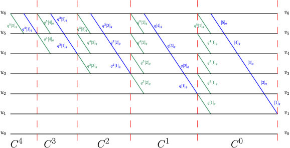
Figure 9. The planar network ${\mathcal{N}}_{2}$ up to source $u_{6}$ and sink $v_{6}$. Note that the dashed red lines do not form part of the network, they simply delineate the column transfer matrices of ${\mathcal{N}}_{2}$. Also note that the direction of the edges have been omitted, the reader should assume all edges are directed from left to right.

Proposition 5.1.

The path matrix for ${\mathcal{N}}_{2}$ satisfies

$$P_{{\mathcal{N}}_{2}}\;=\;\mathsf{F}(q).$$ (5.8)

Before beginning the proof proper we first outline our approach. The factorisation of $P_{{\mathcal{N}}_{2}}$ in (5.7) is of the form

$$\cdots(L_{4}T_{4})(L_{3}T_{3})(L_{2}T_{2})(L_{1}T_{1}),$$ (5.9)

where $L_{i}$ denotes a lower-bidiagonal matrix $L$ downshifted by $i$:

$$L_{i}\;=\left[\begin{array}[]{c|c}I_{i}&0\\ \hline\cr 0&L\end{array}\right],$$ (5.10)

and similarly $T_{i}$ denotes an inverse lower-bidiagonal matrix $T$ downshifted by $i$:

$$T_{i}\;=\;\left[\begin{array}[]{c|c}I_{i}&0\\ \hline\cr 0&T\end{array}\right].$$ (5.11)

Applying Lemma 2.9 to the rightmost product $L_{1}T_{1}$ we obtain

$$L_{1}T_{1}\;=\;T_{2}^{\prime}L_{1}^{\prime},$$ (5.12)

where $T_{2}^{\prime}$ is an inverse lower-bidiagonal matrix downshifted by $2$ and $L_{1}^{\prime}$ a lower-bidiagonal matrix downshifted by $1$. The factorisation in (5.9) can therefore be expressed as

$$\cdots(L_{4}T_{4})(L_{3}T_{3})(L_{2}T_{2}T_{2}^{\prime})L_{1}^{\prime}.$$ (5.13)

More generally, Lemma 2.9 enables us to “pull” lower-bidiagonal matrices “through” inverse lower-bidiagonal matrices to the right (compare Figure 6 with Figure 9), so that in particular for a given $i>0$ the factorisation in 5.9 can be written in the form

$$\cdots(L_{i+2}T_{i+2})\left(L_{i+1}T_{i+1}\prod_{j=1}^{i}T_{i+1,j}\right)L_{i}^{\prime}L_{i-1}^{\prime}\cdots L_{1}^{\prime}$$ (5.14)

where each $T_{i+1,j}$ is an inverse bidiagonal matrix downshifted by $i+1$, and each $L_{i}^{\prime}$ is a lower-bidiagonal matrix downshifted by $i$. It is clear that in the limit (as $i\to\infty$) the inverse lower-bidiagonal matrices disappear, and what remains is a factorisation of $P_{{\mathcal{N}}_{2}}$ into downshifted lower-bidiagonal matrices:

$$P_{{\mathcal{N}}_{2}}\;=\;\cdots L_{4}^{\prime}L_{3}^{\prime}L_{2}^{\prime}L_{1}^{\prime}.$$ (5.15)

We will show that this resulting factorisation of $P_{{\mathcal{N}}_{2}}$ agrees with the production-like factorisation of $\mathsf{F}(q)$ given in Corollary 4.4 of the previous section.

Proof of Proposition 5.1.

It is easy to see that the matrices agree in the first column, since

$$P_{{\mathcal{N}}_{2}}(u_{n}\to v_{0})\;=\;\delta_{n0}\;=\;f_{n,0}(q),$$ (5.16)

so consider again the matrix

$$\mathsf{F}^{\prime}(q)\coloneqq(f^{\prime}_{n,k}(q))_{n,k\geq 0}\;=\;\left(\genfrac{(}{)}{0.0pt}{}{n}{k}_{q}([n+1]_{q})^{n-k}\right)_{n,k\geq 0}$$ (5.17)

and let ${\mathcal{N}}_{2}^{\prime}$ denote the planar network obtained by removing from ${\mathcal{N}}_{2}$ vertices $u_{0},v_{0}$ and relabelling vertices $u_{i}\to u_{i-1}$, $v_{i}\to v_{i-1}$ for $i>0$ (the corresponding path matrix $P_{{\mathcal{N}}_{2}^{\prime}}$ is thus obtained by deleting the first row and column of $P_{{\mathcal{N}}_{2}}$).

As described above, we will prove (5.8) by repeatedly applying Lemma 2.9 to the matrix factorisation of $P_{{\mathcal{N}}_{2}^{\prime}}$, thereby expressing $P_{{\mathcal{N}}_{2}}$ as a product of lower-bidiagonal matrices that agree with those given in Corollary 4.4. To this end, fix $i\geq 0$ and consider the product

$$P^{\prime}_{C^{i}}\cdots P^{\prime}_{C^{1}}P^{\prime}_{C^{0}}\;=\;\left[\begin{array}[]{c|c}I_{i}&0\\ \hline\cr 0&L({\mathbf{a}}_{i}(q))T({\mathbf{b}}_{i}(q))\end{array}\right]\cdots\left[\begin{array}[]{c|c}1&0\\ \hline\cr 0&L({\mathbf{a}}_{1}(q))T({\mathbf{b}}_{1}(q))\end{array}\right]\cdot L({\mathbf{a}}_{0}(q))T({\mathbf{b}}_{0}(q))$$ (5.18)

where

$${\mathbf{a}}_{i}(q)\;=\;(q^{i+n+1}[i+1]_{q})_{n\geq 0}$$ (5.19)

and

$${\mathbf{b}}_{i}(q)\;=\;(q^{i}[n+1]_{q})_{n\geq 0}$$ (5.20)

(each matrix $P^{\prime}_{C^{i}}$ is obtained by deleting the first row and column from $P_{C^{i}}$ defined in (5.4) above).

Claim 1. We claim that

$$P^{\prime}_{C^{i}}\cdots P^{\prime}_{C^{1}}P^{\prime}_{C^{0}}\;=\;\left[\begin{array}[]{c|c}I_{i+1}&0\\ \hline\cr 0&{\bf T}^{i}(q)\end{array}\right]\cdot\left[\begin{array}[]{c|c}I_{i}&0\\ \hline\cr 0&L({\mathbf{c}}_{i}(q))\end{array}\right]\cdots\left[\begin{array}[]{c|c}1&0\\ \hline\cr 0&L({\mathbf{c}}_{1}(q))\end{array}\right]L({\mathbf{c}}_{0}(q))$$ (5.21)

where

$${\bf T}^{i}(q)=\prod_{j=0}^{i}T({\mathbf{b}}_{i,j}(q))$$ (5.22)

is a product of inverse bidiagonal matrices with corresponding edge sequences

$${\mathbf{b}}_{i,j}(q)\coloneqq\left(q^{i-j}[n+1]_{q}\left(\frac{[n+i+3]_{q}}{[n+i+2]_{q}}\right)^{j+1}\right)_{n\geq 0}$$ (5.23)

and each $L({\mathbf{c}}_{i}(q))$ is the lower-bidiagonal matrix with edge sequence

$${\mathbf{c}}_{i}(q)\;=\;\left(q^{n}[i+1]_{q}\left(\frac{[n+i+2]_{q}}{[n+i+1]_{q}}\right)^{i+1}\right)_{n\geq 0}.$$ (5.24)

Please note that the lower-bidiagonal matrices $L({\mathbf{c}}_{i}(q))$ are obtained by deleting the first row and column of the matrices found in the production-like factorisation of $\mathsf{F}(q)$ in Corollary 4.4 above, so proof of the proposition follows once we have proved the claim (since (5.21) implies that for $0\leq n\leq i+1$, each $(n,k)$-entry of $P^{\prime}_{C^{i}}\cdots P^{\prime}_{C^{1}}P^{\prime}_{C^{0}}$ agrees with that of $\mathsf{F}^{\prime}(q)$).

First observe that we can apply Lemma 2.9 to the product $L({\mathbf{a}}_{i}(q))T({\mathbf{b}}_{i}(q))$ in $P^{\prime}_{C^{i}}$, yielding

$$P^{\prime}_{C^{i}}\;=\;\left[\begin{array}[]{c|c}I_{i+1}&0\\ \hline\cr 0&T({\mathbf{b}}^{\prime}_{i}(q))\end{array}\right]\cdot\left[\begin{array}[]{c|c}I_{i}&0\\ \hline\cr 0&L({\mathbf{a}}^{\prime}_{i}(q))\end{array}\right]$$ (5.25)

where

$${\mathbf{a}}^{\prime}_{i}(q)\coloneqq\left(\frac{q^{i+n}[i+1]_{q}[n+i+2]_{q}}{[n+i+1]_{q}}\right)_{n\geq 0},$$ (5.26)

and

$${\mathbf{b}}^{\prime}_{i}(q)\coloneqq\left(\frac{q^{i}[n+1]_{q}[n+i+3]_{q}}{[n+i+2]_{q}}\right)_{n\geq 0}.$$ (5.27)

Clearly $T({\mathbf{b}}^{\prime}_{i}(q))=T({\mathbf{b}}_{i,0}(q))$, moreover it is easily verified that ${\mathbf{a}}^{\prime}_{0}(q)={\mathbf{c}}_{0}(q)$, so suppose (5.21) holds for $i-1\geq 0$. By the induction hypothesis and (5.25) we have

$$P^{\prime}_{C^{i}}\cdots P^{\prime}_{C^{0}}=\left[\begin{array}[]{c|c}I_{i+1}&0\\ \hline\cr 0&T({\mathbf{b}}_{i,0}(q))\end{array}\right]\cdot\left[\begin{array}[]{c|c}I_{i}&0\\ \hline\cr 0&L({\mathbf{a}}^{\prime}_{i}(q)){\bf T}^{(i-1)}(q)\end{array}\right]\cdot\left[\begin{array}[]{c|c}I_{i-1}&0\\ \hline\cr 0&L({\mathbf{c}}_{i-1}(q))\end{array}\right]\cdots L({\mathbf{c}}_{0}(q)).$$ (5.28)

We now make the following claim:

Claim 2. For $0\leq m\leq i-1$,

$$L({\mathbf{a}}^{\prime}_{i}(q))\prod_{j=0}^{m}T({\mathbf{b}}_{i-1,j}(q))\;=\;\left[\begin{array}[]{c|c}1&0\\ \hline\cr 0&T({\mathbf{b}}_{i,1}(q))\cdots T({\mathbf{b}}_{i,m+1}(q))\end{array}\right]\cdot L({\mathbf{c}}^{\prime}_{m+1}(q))$$ (5.29)

where ${\mathbf{c}}^{\prime}_{m}(q)$ is the edge sequence

$${\mathbf{c}}^{\prime}_{m}(q)\coloneqq\left(q^{i+n-m}[i+1]_{q}\left(\frac{[n+i+2]_{q}}{[n+i+1]_{q}}\right)^{m+1}\right)_{n\geq 0}.$$ (5.30)

Claim 2  (5.29) clearly holds for $m=0$ by way of Lemma 2.9:

$$L({\mathbf{a}}^{\prime}_{i}(q))T({\mathbf{b}}_{i-1,0}(q))=\left[\begin{array}[]{c|c}1&0\\ \hline\cr 0&T({\mathbf{b}}_{i,1}(q))\end{array}\right]\cdot L({\mathbf{c}}^{\prime}_{1}(q)),$$ (5.31)

and more generally we have (again by Lemma 2.9)

$$L({\mathbf{c}}^{\prime}_{m}(q))T({\mathbf{b}}_{i-1,m}(q))=\left[\begin{array}[]{c|c}1&0\\ \hline\cr 0&T({\mathbf{b}}_{i,m+1}(q))\end{array}\right]\cdot L({\mathbf{c}}^{\prime}_{m+1}(q)).$$ (5.32)

Letting $m=i-1$ above proves Claim 2 (5.29), which in turn confirms Claim 1 (5.21) since it is straightforward to check that ${\mathbf{c}}^{\prime}_{i}(q)={\mathbf{c}}_{i}(q)$, thereby completing the proof of the proposition.

∎

Coefficientwise total positivity of $\mathsf{F}(q)$ and ${\sf T}(q)$ follows almost immediately from Proposition 5.1:

Proof of Theorem 1.2.

Since ${\mathcal{N}}_{2}$ is a planar network with weights that are polynomials with nonnegative coefficients in $q$ and we have just shown that $P_{{\mathcal{N}}_{2}}=\mathsf{F}(q)$, the matrix $\mathsf{F}(q)$ is coefficientwise totally positive in ${\mathbb{Z}}[q]$ thanks to the LGV lemma. The coefficientwise total positivity of ${\sf T}(q)$ then follows from the fact that

$${\sf T}(q)\;=\;\mathsf{F}(q)T((q^{n}[n+1]_{q})_{n\geq 0})$$ (5.33)

(see Lemma 3.11 above), since the inverse lower-bidiagonal matrix $T((q^{n}[n+1]_{q})_{n\geq 0})$ is coefficientwise totally positive. ∎

Proving Theorem 1.2 was the main goal of this paper, however, the planar network ${\mathcal{N}}_{2}$ can be seen as a specialisation of a more general network that appears to satisfy some interesting properties that we believe warrant further investigation. We discuss this more general network in the following section.

6. Further comments and some open problems

In this final section we turn our attention to a generalisation of the planar network ${\mathcal{N}}_{2}$ that under certain specialisations yield matrices with entries that appear to count a variety of combinatorial objects with respect to different statistics. These matrices are automatically coefficientwise totally positive, since they arise from planar networks with weights that are polynomials with nonnegative coefficients. Furthermore, under certain specialisations, sequences of row-generating polynomials related to these matrices turn out to be sequences of polynomials that are already well-known, and in some cases are also known to be coefficientwise Hankel-totally positive (a sequence ${\mathbf{a}}=(P_{n}({\mathbf{x}}))_{n\geq 0}$ of polynomials in one or more indeterminates ${\mathbf{x}}$ is coefficientwise Hankel-totally positive if its associated Hankel matrix $H_{\infty}({\mathbf{a}})\coloneqq(P_{n+k}({\mathbf{x}}))_{n,k\geq 0}$ is coefficientwise totally positive in all the indeterminates ${\mathbf{x}}$).

We will briefly touch upon the method of production matrices (see [18, 19]), which in recent years has become an important tool in enumerative combinatorics and has its roots in Stieltjes’ work on continued fractions. The theory of production matrices with respect to total positivity is extensively studied in [64], however, since [64] is not yet publicly available we direct the reader to Sections 2.2 and 2.3 of [66] for a fuller treatment.

For our purposes we will require the following principles: let $\mathsf{P}=(p_{i,j})_{i,j\geq 0}$ be an infinite matrix with entries in ${\mathbb{R}}[{\mathbf{x}}]$ equipped with the coefficientwise order. In order that powers of $\mathsf{P}$ are well defined we assume that $\mathsf{P}$ is either row finite (that is, has only finitely many nonzero entries in each row) or column finite. Let us now define the infinite matrix $A\coloneqq(a_{n,k})_{n,k\geq 0}$ where

$$a_{n,k}=(\mathsf{P}^{n})_{0,k},$$ (6.1)

that is, row $n$ of $A$ is the first row of the matrix power $\mathsf{P}^{n}$ (in particular we set $a_{0,k}=\delta_{0k}$). We call $\mathsf{P}$ the production matrix of $A$, while $A$ is referred to as the output matrix of $\mathsf{P}$ and we write ${\mathcal{O}}(\mathsf{P})=A$. The entries of $A$ are, explicitly,

$$a_{n,k}\;=\;\sum_{i_{1},\ldots,i_{n-1}}p_{0,i_{1}}p_{i_{1},i_{2}}p_{i_{2},i_{3}}\cdots p_{i_{n-2},i_{n-1}}p_{i_{n-1},k},$$ (6.2)

which can be seen as the total weight of all $n$-step walks in ${\mathbb{N}}$ from $i_{0}=0$ to $i_{n}=k$, in which the weight of a walk is the product of the weights of its steps, and each step from $i$ to $j$ has weight $p_{i,j}$. An equivalent formulation is to define the entries by the recurrence

$$a_{n,k}\;=\;\sum_{i=0}^{\infty}a_{n-1,i}p_{i,k}$$ (6.3)

for $n\geq 1$ with initial condition $a_{0,k}\;=\;\delta_{0k}$.

Given a production matrix $\mathsf{P}$, we define the augmented production matrix to be

$$\tilde{\mathsf{P}}\;\coloneqq\;\left[\begin{array}[]{c}1\,\,0\,\,0\,\,0\,\,\cdots\\ \hline\cr\mathsf{P}\end{array}\right],$$ (6.4)

and it is easy to show [66, Section 2.2] that the output matrix of $\mathsf{P}$ has the factorisation

$${\mathcal{O}}(\mathsf{P})\;=\;\cdots\left[\begin{array}[]{c|c}I_{3}&0\\ \hline\cr 0&\tilde{\mathsf{P}}\end{array}\right]\cdot\left[\begin{array}[]{c|c}I_{2}&0\\ \hline\cr 0&\tilde{\mathsf{P}}\end{array}\right]\cdot\left[\begin{array}[]{c|c}1&0\\ \hline\cr 0&\tilde{\mathsf{P}}\end{array}\right]\tilde{P}.$$ (6.5)

Clearly if $\mathsf{P}$ is coefficientwise totally positive then so is $\tilde{\mathsf{P}}$, and hence so is ${\mathcal{O}}(\mathsf{P})$ (Theorem 2.9 in [66]). The factorisation given above is the reason we call the factorisation in Corollary 2.4 production-like. The quasi-production-like factorisation in Corollary 2.7 is named after the related concept of quasi-production matrices (see [10]) that we do not require here.

6.1. General Abel Polynomials

Let us now return to the $q$-forests matrix $\mathsf{F}(q)$ and consider the matrix

$$\bar{\mathsf{F}}(q)\coloneqq(\bar{f}_{n,k}(q))_{n,k\geq 0}\;=\;\mathsf{F}(q)\mathop{\rm diag}\nolimits((q^{n(n-1)/2})_{n\geq 0}),$$ (6.6)

the row-generating polynomials of which are defined to be

$$\bar{\mathsf{F}}_{0}(x;q)\coloneqq 1$$ (6.7)

and

$$\bar{\mathsf{F}}_{n}(x;q)\coloneqq\sum_{k=0}^{n}\bar{f}_{n,k}(q)x^{k}\;=\;\sum_{k=0}^{n}\genfrac{(}{)}{0.0pt}{}{n-1}{k-1}_{q}([n]_{q})^{n-k}x^{k}$$ (6.8)

for $n>0$. By employing the finite sum version of the $q$-binomial theorem [2, Theorem 3.3]:

$$\sum_{k=0}^{n}\genfrac{(}{)}{0.0pt}{}{n}{k}_{q}(-z)^{k}q^{\binom{k+1}{2}}\;=\;\prod_{i=0}^{n-1}(1-zq^{i}),$$ (6.9)

in which $z$ has been replaced with $(-qx/[n]_{q})$, we obtain the explicit formulas

$$\bar{\mathsf{F}}_{0}(x;q)\;=\;1$$ (6.10)

and

$$\bar{\mathsf{F}}_{n}(x;q)\;=\;x\prod_{i=1}^{n-1}(xq^{i}+[n]_{q}).$$ (6.11)

For $q$ specialised to $q=1$ the polynomials $\bar{\mathsf{F}}(x;1)$ reduce to the Abel polynomials

$$\bar{\mathsf{F}}_{n}(x;1)\;=\;x(x+n)^{n-1},$$ (6.12)

which are the row-generating polynomials of the forests matrix $\mathsf{F}$. Sokal [66] has already proven that the Abel polynomials (along with further generalisations of the row-generating polynomials of the forests matrix) are coefficientwise Hankel-totally positive. It is natural to ask, then, whether this property is preserved if $q$ is left as an indeterminate in $\bar{\mathsf{F}}_{n}(x;q)$.

The Hankel matrix associated to $\bar{\mathsf{F}}_{n}(x;q)$,

$$H_{\infty}((\bar{\mathsf{F}}_{n}(x;q))_{n\geq 0})=(\pi_{n,k})_{n,k\geq 0},$$ (6.13)

begins:

$$\left[\begin{array}[]{ccc}x&x(qx+q+1)&\cdots\\ x(qx+q+1)&x\left(q^{2}+qx+q+1\right)\left(q^{2}x+q^{2}+q+1\right)&\cdots\\ \vdots&\vdots&\ddots\end{array}\right]$$ (6.14)

which contains the $2\times 2$ minor

$$\pi_{0,0}\pi_{1,1}-\pi_{1,0}\pi_{0,1}\;=\;2q^{2}x^{2}+2q^{3}x^{2}+q^{4}x^{2}-qx^{3}+2q^{3}x^{3}+q^{4}x^{3}-q^{2}x^{4}+q^{3}x^{4}\not\succeq 0,$$ (6.15)

so our generalisation does not preserve coefficientwise Hankel-total positivity. By studying the minor above, however, one might suppose that shifting $q$ by $1$ (that is, replacing $q$ with $1+r$) might yield a polynomial sequence $(\bar{\mathsf{F}}_{n}(x;1+r))_{n\geq 0}$ that is coefficientwise Hankel-totally positive; indeed, computer experiments conducted with Alan Sokal seem to confirm this for $n\leq 10$. We conjecture:

Conjecture 6.1 (with Alan Sokal).

The polynomial sequence $(\bar{\mathsf{F}}_{n}(x;1+r))_{n\geq 0}$ is coefficientwise Hankel-totally positive jointly in $x$ and $r$.

In the following subsections we consider further generalisations of the forests matrix to more indeterminates, and a common theme begins to emerge; in each case we have observed that modifying these matrices in a similar way to (6.6) above and shifting the indeterminates by $1$ yields a set of matrices with row-generating polynomials that appear to be coefficientwise Hankel-totally positive jointly in a number of indeterminates.

The polynomials $\bar{\mathsf{F}}_{n}(x;q)$ are, in fact, specialisations of a $q$-generalisation of the general Abel polynomials presented in [13, 37, 38]:

$$a_{0}(x;b,h,w,q) \coloneqq 1$$ (6.16)

$$a_{n}(x;b,h,w,q) \coloneqq (x+b)\prod_{i=1}^{n-1}(xq^{i}+b+[i]_{q}h+[n]_{q}w)\vskip 12.0pt plus 4.0pt minus 4.0pt\textrm{ for }n\geq 1.$$ (6.17)

Note that for $w=1$, $b=h=0$ the above formula gives a $q$-generalisation of the Stirling cycle polynomials, so the polynomials $a_{n}(x;b,h,w,q)$ interpolate between $q$-forest polynomials and a $q$-generalisation of the Stirling cycle polynomials (below we will consider a different $q$-generalisation of the Stirling cycle polynomials).

Johnson [38, Section 4] showed that the polynomials $a_{n}(x;b,h,w,q)$ are of $q$-binomial type, that is, they satisfy

$$a_{n}(x;a+b,h,w,q)\;=\;\sum_{k=0}^{n}\genfrac{(}{)}{0.0pt}{}{n}{k}_{q}a_{n-k}(0;a,h+(1-q)(b+[k]_{q}w),w(1-(1-q)[k]_{q}))\\ \times a_{k}(x;a,h,w,q)$$ (6.18)

and

$$a_{n}(x+y;a+b,0,w,q)\;=\;\sum_{k=0}^{n}\genfrac{(}{)}{0.0pt}{}{n}{k}_{q}a_{n-k}(yq^{k};a,(1-q)(b+[k]_{q}w),w(1-(1-q)[k]_{q}))\\ \times a_{k}(x;a,0,w,q).$$ (6.19)

The identities above are $q$-extensions of an identity that goes back to Rothe [59] in 1793 and Pfaff [50] in 1795, usually expressed as:

$$R_{n}(x+y;h,w)\;=\;\sum_{k=0}^{n}\binom{n}{k}R_{k}(x;h,w)R_{n-k}(y;h,w)$$ (6.20)

where

$$R_{0}(x;h,w)\coloneqq 1$$ (6.21)

and

$$R_{n}(x;h,w)\coloneqq x\prod_{i=1}^{n-1}(x+ih+nw)$$ (6.22)

for $n>0$.

In [66, Section 6] Sokal explains how these polynomials are a rewriting of the Schläfli-Gessel-Seo polynomials:

$$P_{0}(x;a,b)\coloneqq 1$$ (6.23)

and

$$P_{n}(x;a,b)\coloneqq x\prod_{i=1}^{n-1}(x+ai+(n-i)b)$$ (6.24)

which were introduced by Schläfli in 1847 [61], and resurfaced much later in a 2006 paper by Gessel and Seo [31] who showed that

$$P_{n,k}(a,b)\;=\;[x^{k}]P_{n}(x;a,b)$$ (6.25)

enumerates $k$-component forests on the vertex set $[n]$ by proper and improper vertices, and also by ascents and descents. Sokal’s paper contains a fuller discussion of these polynomials as well as a number of interesting conjectures regarding their coefficientwise Hankel-total positivity, and we enthusiastically encourage the reader to consult the final section of [66] for further details.

There is, unsurprisingly, something of an overlap between this current paper and the generalisations of the forest matrix studied by Sokal [66]. In the next subsection we will show how our planar network ${\mathcal{N}}_{2}$ from Section 5 can be modified to derive some of the results proven in [66].

6.2. Enumerating forests by proper and improper edges

In [66] Sokal considers total positivity properties of generalisations of the forests matrix that differs from the $q$-generalisations studied in this paper. We will now show how making some simple modifications to the planar network ${\mathcal{N}}_{2}$ yields a path matrix that agrees with one of the generalisations studied in [66].

Given two vertices $i$ and $j$ of a tree $T$ belonging to a forest, we say that $j$ is a descendant of $i$ if the unique path from the root of $T$ to $j$ passes through $i$ (note that every vertex is a descendant of itself). Let $e=ij$ be an edge of $T$. We say that $e$ is improper if there is a descendant of $j$ (possibly $j$ itself) that is lower-numbered than $i$, otherwise we say that $e$ is proper (see Section 1 of [66]).

Consider the matrix

$$\mathsf{F}(y,z)\;\coloneqq\;(f_{n,k}(y,z))_{n,k\geq 0},$$ (6.26)

the entries of which are given by

$$f_{n,k}(y,z)\;\coloneqq\;\sum_{m=0}^{n-k}f_{n,k,m}y^{m}z^{n-k-m}$$ (6.27)

where $f_{n,k,m}$ is the number of forests of rooted trees on the vertex set $[n]$ that have $k$ components and $m$ improper edges. The first few rows of $\mathsf{F}(y,z)$ are:

$$\left[\begin{array}[]{cccccc}1&&&&&\\ 0&1&&&&\\ 0&y+z&1&&&\\ 0&3y^{2}+4yz+2z^{2}&3y+3z&1&&\\ 0&25y^{2}z+15y^{3}+18yz^{2}+6z^{3}&15y^{2}+22yz+11z^{2}&6y+6z&1&\\ \vdots&\vdots&\vdots&\vdots&\vdots&\ddots\\ \end{array}\right],$$ (6.28)

each entry is a homogeneous polynomial of degree $n-k$, and under the specialisation $y=z=1$ we recover the forests matrix (that is, $\mathsf{F}(1,1)=\mathsf{F}$). Sokal also observes (see the remark on page 7 of [66]) that the polynomials $f_{n,1}(y,z)$ (which enumerate rooted trees with respect to improper edges) are homogenised versions of the Ramanujan polynomials (see [9, 20, 35, 36, 40, 45, 55, 62, 75] and [63, A054589]).

The matrix $\mathsf{F}(y,z)$ is the exponential Riordan array ${\mathcal{R}}[F,G^{\prime}]$ with $F(t)=1$ and

$$G^{\prime}(t)\;=\;\frac{1}{z}\left[G\left(\left(1-\frac{z}{y}+\frac{z^{2}}{y}t\right)e^{-\left(1-\frac{z}{y}\right)}\right)-\left(1-\frac{z}{y}\right)\right]$$ (6.29)

(Section 3.2 of [66]) where $G(t)$ is the tree function (see [16] and (1.11) above). Sokal proved that $\mathsf{F}(y,z)$ is coefficientwise totally positive in ${\mathbb{Z}}[y,z]$ using the production-matrix method; the production matrix for $\mathsf{F}(y,z)$ is the lower-Hessenberg matrix $\mathsf{P}(y,z)\coloneqq(p_{n,k}(y,z))_{n,k\geq 0}$ with entries

$$p_{n,k}(y,z)\;=\;\frac{n!}{(k-1)!}\sum_{l=0}^{n+1-k}\frac{y^{n-l}z^{l}}{l!}$$ (6.30)

(see [66, Proposition 4.7]). The first few rows of $\mathsf{P}(y,z)$ are:

$$\left[\begin{array}[]{cccccc}0&1&&&&\\ 0&y+z&y&&&\\ 0&2y^{2}+2yz+z^{2}&2y^{2}+2yz&y^{2}&&\\ 0&6y^{2}z+6y^{3}+3yz^{2}+z^{3}&6y^{2}z+6y^{3}+3yz^{2}&3y^{2}z+3y^{3}&y^{3}&\\ \vdots&\vdots&\vdots&\vdots&\vdots&\ddots\end{array}\right],$$ (6.31)

and $\mathsf{P}(y,z)$ has the factorisation [66, Proposition 4.8]

$$\mathsf{P}(y,z)\;=\;B_{z}\mathop{\rm diag}\nolimits((n!)_{n\geq 0})T_{\infty}(y)\mathop{\rm diag}\nolimits((k!)_{k\geq 0})^{-1}\Delta,$$ (6.32)

where $T_{\infty}(y)$ is the Toeplitz matrix of powers of $y$ (see Subsection 2.3 above) and $\Delta\coloneqq(\delta_{n+1,k})_{n,k\geq 0}$ is the lower-Hessenberg matrix with $1$ on the superdiagonal and $0$ elsewhere.

As described above (see (6.5)), the augmented production matrix

$$\tilde{\mathsf{P}}(y,z)\;\coloneqq\;\left[\begin{array}[]{c}1\,\,0\,\,0\,\,0\,\,\cdots\\ \hline\cr\mathsf{P}(y,z)\end{array}\right]$$ (6.33)

with $\mathsf{P}(y,z)$ defined previously yields the following factorisation of $\mathsf{F}(y,z)$:

$$\mathsf{F}(y,z)\;=\;\cdots\left[\begin{array}[]{c|c}I_{3}&0\\ \hline\cr 0&B_{z}T({\bf y}^{*})\end{array}\right]\cdot\left[\begin{array}[]{c|c}I_{2}&0\\ \hline\cr 0&B_{z}T({\bf y}^{*})\end{array}\right]\cdot\left[\begin{array}[]{c|c}1&0\\ \hline\cr 0&B_{z}T({\bf y}^{*})\end{array}\right]$$ (6.34)

where ${\bf y}^{*}=((n+1)y)_{n\geq 0}$ [equivalently, $T({\bf y}^{*})=D\mathop{\rm diag}\nolimits((n!)_{n\geq 0})T_{\infty}(y)\mathop{\rm diag}\nolimits((k!)_{k\geq 0}))^{-1}$] and $B_{z}=B_{z,1}$ is the weighted binomial matrix $B_{x,y}$ with $x=z$ and $y=1$. A diagram of the corresponding planar network ${\mathcal{N}}_{3}$ can be found in Figure 10.

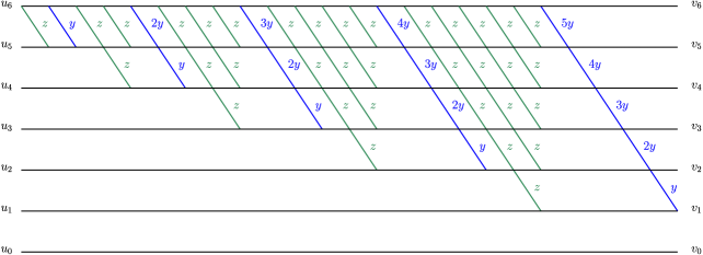
Figure 10. The planar network ${\mathcal{N}}_{3}$ arising from the production-matrix approach used in [66] (unlabelled edges have weight 1).

Now let ${\mathcal{N}}_{4}$ denote the planar network in Figure 11, the corresponding path matrix of which has the production-like factorisation

$$P_{{\mathcal{N}}_{4}}\;=\;\cdots\left[\begin{array}[]{c|c}I_{3}&0\\ \hline\cr 0&L(3z)T({\bf y}^{*})\end{array}\right]\cdot\left[\begin{array}[]{c|c}I_{2}&0\\ \hline\cr 0&L(2z)T({\bf y}^{*})\end{array}\right]\cdot\left[\begin{array}[]{c|c}1&0\\ \hline\cr 0&L(z)T({\bf y}^{*})\end{array}\right]$$ (6.35)

where $L(iz)$ denotes the lower-bidiagonal matrix with 1 on the diagonal, $iz$ on the subdiagonal, and $0$ everywhere else. Comparing Figure 9 in Section 5 with Figure 11 it is easy to see that we obtain ${\mathcal{N}}_{4}$ from ${\mathcal{N}}_{2}$ by specialising $q=1$ and multiplying the weights of the blue and green edges by $y$ and $z$ respectively. We make the following proposition:

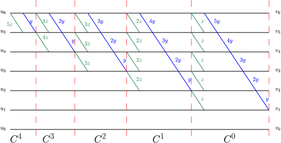
Figure 11. The planar network ${\mathcal{N}}_{4}$ up to source and sink vertices $u_{6}$ and $v_{6}$.

Proposition 6.2.

The path matrix corresponding to ${\mathcal{N}}_{4}$ satisfies

$$P_{{\mathcal{N}}_{4}}\;=\;\mathsf{F}(y,z).$$ (6.36)

Proof.

Consider the factorisation of $\mathsf{F}(y,z)$ in (6.34) above:

$$\mathsf{F}(y,z)\;=\;\cdots\left[\begin{array}[]{c|c}I_{3}&0\\ \hline\cr 0&B_{z}T({\bf y}^{*})\end{array}\right]\cdot\left[\begin{array}[]{c|c}I_{2}&0\\ \hline\cr 0&B_{z}T({\bf y}^{*})\end{array}\right]\cdot\left[\begin{array}[]{c|c}1&0\\ \hline\cr 0&B_{z}T({\bf y}^{*})\end{array}\right].$$ (6.37)

The matrix $B_{z}$ has the production-like factorisation

$$B_{z}\;=\;\cdots\left[\begin{array}[]{c|c}I_{3}&0\\ \hline\cr 0&L(z)\end{array}\right]\cdot\left[\begin{array}[]{c|c}I_{2}&0\\ \hline\cr 0&L(z)\end{array}\right]\cdot\left[\begin{array}[]{c|c}1&0\\ \hline\cr 0&L(z)\end{array}\right]L(z)\;=\;\left[\begin{array}[]{c|c}1&0\\ \hline\cr 0&B_{z}\end{array}\right]\cdot L(z)$$ (6.38)

(see Corollary 2.5 with $y=1$ and $x$ replaced with $z$, and also observe that the right-hand side above implies that $L(z)$ is the augmented production matrix of $B_{z}$). It follows that

$$\mathsf{F}(y,z)\;=\;\cdots\left[\begin{array}[]{c|c}I_{3}&0\\ \hline\cr 0&B_{z}T({\bf y}^{*})\end{array}\right]\cdot\left[\begin{array}[]{c|c}I_{2}&0\\ \hline\cr 0&B_{z}T({\bf y}^{*})B_{z}\end{array}\right]\cdot\left[\begin{array}[]{c|c}1&0\\ \hline\cr 0&L(z)T({\bf y}^{*})\end{array}\right].$$ (6.39)

A straightforward calculation confirms that

$$T({\bf y}^{*})B_{z}\;=DT_{\infty}(y)D^{-1}DT_{\infty}((z^{n}/n!)_{n\geq 0})D^{-1}\;=\;DT_{\infty}((z^{n}/n!)_{n\geq 0})D^{-1}DT_{\infty}(y)D^{-1}\\ \;=\;B_{z}T({\bf y}^{*})$$ (6.40)

where $D=\mathop{\rm diag}\nolimits((n!)_{n\geq 0})$, since Toeplitz matrices matrices commute:

$$T_{\infty}({\mathbf{a}})T_{\infty}({\mathbf{b}})\;=\;T_{\infty}({\mathbf{a}}*{\mathbf{b}})\;=\;T_{\infty}({\mathbf{b}})T_{\infty}({\mathbf{a}})$$ (6.41)

where ${\mathbf{a}}*{\mathbf{b}}$ is the convolution of the sequences ${\mathbf{a}}$ and ${\mathbf{b}}$

$${\mathbf{a}}*{\mathbf{b}}\;=\;\left(\sum_{k=0}^{n}a_{k}b_{n-k}\right)_{n\geq 0}.$$ (6.42)

Furthermore, it is easily verified that

$$B_{z}B_{z^{\prime}}\;=\;B_{z+z^{\prime}}\;=\;\left[\begin{array}[]{c|c}1&0\\ \hline\cr 0&B_{z+z^{\prime}}\end{array}\right]\cdot L(z+z^{\prime}),$$ (6.43)

hence

$$\mathsf{F}(y,z)\;=\;\cdots\left[\begin{array}[]{c|c}I_{3}&0\\ \hline\cr 0&B_{z}T({\bf y}^{*})B_{2z}\end{array}\right]\cdot\left[\begin{array}[]{c|c}I_{2}&0\\ \hline\cr 0&L(2z)T({\bf y}^{*})\end{array}\right]\cdot\left[\begin{array}[]{c|c}1&0\\ \hline\cr 0&L(z)T({\bf y}^{*})\end{array}\right].$$ (6.44)

Iteratively commuting $T({\bf y}^{*})$ with $B_{iz}$ and writing

$$B_{z}B_{iz}\;=\;\left[\begin{array}[]{c|c}1&0\\ \hline\cr 0&B_{(i+1)z}\end{array}\right]L((i+1)z)$$ (6.45)

for increasing $i$ in the factorisation of $\mathsf{F}(y,z)$ given above completes the proof. ∎

The focus of this paper has been $q$-generalisations of the forests and trees matrices, and note that we can easily introduce $q$-weights into the planar network ${\mathcal{N}}_{3}$. Consider the network ${\mathcal{N}}_{5}$ in Figure 12, which has the corresponding path matrix

$$P_{{\mathcal{N}}_{5}}\;=\;\cdots\left[\begin{array}[]{c|c}I_{3}&0\\ \hline\cr 0&B_{q;z}T((y[n+1]_{q})_{n\geq 0})\end{array}\right]\cdot\left[\begin{array}[]{c|c}I_{2}&0\\ \hline\cr 0&B_{q;z}T((y[n+1]_{q})_{n\geq 0})\end{array}\right]\\ \cdot\left[\begin{array}[]{c|c}1&0\\ \hline\cr 0&B_{q;z}T((y[n+1]_{q})_{n\geq 0})\end{array}\right]$$ (6.46)

where $B_{q;z}$ is the $q$-binomial matrix

$$B_{q;z}\;=\;\left(\genfrac{(}{)}{0.0pt}{}{n}{k}_{q}z^{n-k}\right)_{n,k\geq 0}.$$ (6.47)

Now let

$$\hat{\mathsf{F}}(q,y,z)\;=\;(\hat{f}_{n,k}(q,y,z))_{n,k\geq 0}\;=\;P_{{\mathcal{N}}_{5}}$$ (6.48)

and observe that $\hat{\mathsf{F}}(q,y,z)$ is the output matrix of the lower-Hessenberg production matrix $\mathsf{P}^{\prime}(q,y,z)=(p_{n,k}(q,y,z))_{n,k\geq 0}$ where

$$\mathsf{P}^{\prime}(q,y,z)\;=\;D_{q}T_{\infty}((z^{n}/[n]_{q}!)_{n\geq 0})T_{\infty}(y)D_{q}^{-1}\Delta$$ (6.49)

where $D_{q}=\mathop{\rm diag}\nolimits(([n]_{q}!)_{n\geq 0})$.

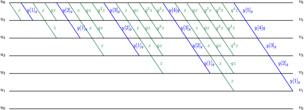
Figure 12. The planar network ${\mathcal{N}}_{5}$, obtained by introducing $q$-weights into the network ${\mathcal{N}}_{3}$.

Define the row-generating polynomials of $\hat{\mathsf{F}}(q,y,z)$ to be:

$$\hat{\mathsf{F}}_{0}(x;q,y,z)\;=\;1$$ (6.50)

and

$$\hat{\mathsf{F}}_{n}(x;q,y,z)\;=\;\sum_{k=0}^{n}\hat{f}_{n,k}(q,y,z)x^{k}$$ (6.51)

for $n\geq 1$. We have the following lemma:

Lemma 6.3.

The sequence $(\hat{\mathsf{F}}_{n}(x;q,y,z))_{n\geq 0}$ of row-generating polynomials of $\hat{\mathsf{F}}(q,y,z)={\mathcal{O}}(\mathsf{P}^{\prime}(q,y,z))$ is coefficientwise Hankel-totally positive jointly in $q,x,y,z$.

In order to prove Lemma 6.3 we first recall two easy results from [66]. The first is:

Lemma 6.4 (Lemma 2.6 in [66]).

Let $P=(p_{i,j})_{i,j\geq 0}$ be a row-finite matrix (with entries in a commutative ring $R$) with output matrix $A={\mathcal{O}}(P)$; and let $B=(b_{i,j})_{i,j\geq 0}$ be a lower-triangular matrix with invertible (in $R$) diagonal entries. Then

$$AB\;=\;b_{0,0}{\mathcal{O}}(B^{-1}PB).$$ (6.52)

That is, up to a factor $b_{0,0},$ the matrix $AB$ has production matrix $B^{-1}PB$.

The second is the following theorem:

Theorem 6.5 (Theorem 2.14 in [66]).

Let $P=(p_{i,j})_{i,j\geq 0}$ be an infinite row-finite or column-finite matrix with entries in a partially ordered commutative ring $R$, and define the infinite Hankel matrix $H_{\infty}({\mathcal{O}}_{0}(P))=((P^{n+n^{\prime}})_{0,0})_{n,n^{\prime}\geq 0}$. If $P$ is totally positive of order $r$, then so is $H_{\infty}({\mathcal{O}}_{0}(P))$.

Our proof of Lemma 6.3 relies on these two useful facts, and follows along the same lines as the argument found in the proof of Lemma 2.16 of [66] where $D$ is replaced with $D_{q}$, $B_{x}$ is replaced with $B_{q;x}$, and

$$\boldsymbol{\phi}\;=\;(\phi_{n})_{n\geq 0}\;=\;\sum_{l=0}^{n}\frac{z^{l}y^{n-l}}{[l]_{q}!}.$$ (6.53)

Proof of Lemma 6.3.

The row-generating polynomials of $\hat{\mathsf{F}}(q,y,z)$ are the entries in the zeroth column of the matrix

$$\hat{\mathsf{F}}^{*}(q,x,y,z)\;=\;\hat{\mathsf{F}}(q,y,z)B_{q;x},$$ (6.54)

and according to Lemma 6.4 above we have

$$\hat{\mathsf{F}}^{*}(q,x,y,z)\;=\;{\mathcal{O}}(B_{q;x}^{-1}\mathsf{P}^{\prime}(q,y,z)B_{q;x}).$$ (6.55)

Since $\mathsf{P}^{\prime}(q,y,z)$ is coefficientwise totally positive it suffices (thanks to Theorem 6.5) to show that the matrix

$$B_{q;x}^{-1}\mathsf{P}^{\prime}(q,y,z)B_{q;x}$$ (6.56)

is coefficientwise totally positive. We have

$$B_{q;x}\;=\;D_{q}T_{\infty}((x^{n}/[n]_{q}!)_{n\geq 0})D_{q}^{-1},$$ (6.57)

and

$$\mathsf{P}^{\prime}(q,y,z)\;=\;D_{q}T_{\infty}(\boldsymbol{\phi})D_{q}^{-1}\Delta,$$ (6.58)

where

$$\boldsymbol{\phi}\;=\;(\phi_{n})_{n\geq 0}\;=\;\sum_{l=0}^{n}\frac{z^{l}y^{n-l}}{[l]_{q}!}.$$ (6.59)

It follows that $B_{q;x}$ and $D_{q}T_{\infty}(\boldsymbol{\phi})D_{q}^{-1}$ commute.

Note further that according to the recurrences for $q$-binomial coefficients (see  (3.45) and (3.46) in Section 3) we have

$$\Delta B_{q;x}\;=\;B_{q;x}(\mathop{\rm diag}\nolimits((q^{n}x)_{n\geq 0})+\Delta).$$ (6.60)

We therefore have

$$B_{q;x}^{-1}\mathsf{P}^{\prime}(q,y,z)B_{q;x} =B_{q;x}^{-1}D_{q}T_{\infty}(\boldsymbol{\phi})D_{q}^{-1}\Delta B_{q;x}$$

$$=B_{q;x}^{-1}D_{q}T_{\infty}(\boldsymbol{\phi})D_{q}^{-1}B_{q;x}(\mathop{\rm diag}\nolimits((q^{n}x)_{n\geq 0})+\Delta)$$

$$=D_{q}T_{\infty}(\boldsymbol{\phi})D_{q}^{-1}(\mathop{\rm diag}\nolimits((q^{n}x)_{n\geq 0})+\Delta)$$

$$=D_{q}T_{\infty}(\boldsymbol{\phi})D_{q}^{-1}\Delta(I+\Delta^{T}\mathop{\rm diag}\nolimits((q^{n}x)_{n\geq 0}))$$

(since $\Delta\Delta^{T}=I$), yielding the identity

$$B^{-1}_{q;x}\mathsf{P}^{\prime}(q,y,z)B_{q;x}\;=\;\mathsf{P}^{\prime}(q,y,z)(I+\Delta^{T}\mathop{\rm diag}\nolimits((q^{n}x)_{n\geq 0})),$$ (6.61)

so $B^{-1}_{q;x}\mathsf{P}^{\prime}(q,y,z)B_{q;x}$ coefficientwise totally positive. This completes the proof. ∎

My experiments suggest that there is a more general principle lurking behind Lemma 6.3, concerning production matrices of $q$-Riordan arrays (see  [12], and also [39, 32]). This will be rigorously addressed in future work; for now we turn our attention to a more general planar network that yields both ${\mathcal{N}}_{2}$ and ${\mathcal{N}}_{4}$ under suitable specialisations.

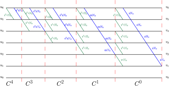
Figure 13. The planar network ${\mathcal{N}}_{6}$.

Consider now the planar network ${\mathcal{N}}_{6}$ in Figure 13 and observe that ${\mathcal{N}}_{4}$ can be obtained from ${\mathcal{N}}_{6}$ by specialising $q=1$ in ${\mathcal{N}}_{6}$ to $q=1$, and by instead specialising $y=z=1$ in ${\mathcal{N}}_{6}$ we obtain the planar network ${\mathcal{N}}_{2}$. The path matrix corresponding to ${\mathcal{N}}_{6}$ has the factorisation:

$$P_{{\mathcal{N}}_{6}}\;=\;\cdots\left[\begin{array}[]{c|c}I_{3}&0\\ \hline\cr 0&L({\mathbf{a}}_{2}(q,z))T({\mathbf{b}}_{2}(q,y))\end{array}\right]\cdot\left[\begin{array}[]{c|c}I_{2}&0\\ \hline\cr 0&L({\mathbf{a}}_{1}(q,z))T({\mathbf{b}}_{1}(q,y))\end{array}\right]\\ \cdot\left[\begin{array}[]{c|c}1&0\\ \hline\cr 0&L({\mathbf{a}}_{0}(q,z))T({\mathbf{b}}_{0}(q,y))\end{array}\right]$$ (6.62)

where

$${\mathbf{a}}_{i}(q,z)\;=\;(q^{n+1+i}z[i+1]_{q})_{n\geq 0}$$ (6.63)

and

$${\mathbf{b}}_{i}(q,y)\;=\;(q^{i}y[n+1]_{q})_{n\geq 0}.$$ (6.64)

Let

$$\tilde{\mathsf{F}}(q,y,z)\;=(\tilde{\mathsf{F}}_{n,k}(q,y,z))_{n,k\geq 0}\;=\;P_{{\mathcal{N}}_{6}}$$ (6.65)

and note that $\tilde{\mathsf{F}}(q,y,z)$ is a generalisation of $\mathsf{F}(q)$ and $\mathsf{F}(y,z)$ in the sense that $\tilde{\mathsf{F}}(1,y,z)=\mathsf{F}(y,z)$, and $\tilde{\mathsf{F}}(q,1,1)=\mathsf{F}(q)$.

Sokal showed in [66] that the row-generating polynomials of $\mathsf{F}(y,z)$:

$$\mathsf{F}_{0}(x;y,z)\coloneqq 1$$ (6.66)

and

$$\mathsf{F}_{n}(x;y,z)\coloneqq\sum_{k=0}^{n}f_{n,k}(y,z)x^{k}$$ (6.67)

for $n>0$ are coefficientwise Hankel-totally positive jointly in $x,y,z$ (Theorem 1.3 of [66]). One might wonder, then, whether the sequence $(\tilde{\mathsf{F}}_{n}(x;q,y,z))_{n\geq 0}$ of row-generating polynomials of $\tilde{\mathsf{F}}(q,y,z)$:

$$\tilde{\mathsf{F}}_{0}(x;q,y,z)\;=\;1$$ (6.68)

and

$$\tilde{\mathsf{F}}_{n}(x;q,y,z)\;=\;\sum_{k=0}^{n}\tilde{f}_{n,k}(q,y,z)x^{k}$$ (6.69)

is also Hankel totally-positive. Unfortunately this is not the case, for the Hankel matrix $H_{\infty}((\tilde{\mathsf{F}}_{n+n^{\prime}})_{n,k\geq 0})=(\pi_{n,k})_{n,k\geq 0}$ contains the $2\times 2$ minor:

$$\pi_{1,0}\pi_{2,1}-\pi_{2,0}\pi_{1,1}=q^{3}x^{2}yz+3q^{2}x^{2}yz+q^{4}x^{2}z^{2}+q^{3}x^{2}z^{2}-q^{2}x^{2}z^{2}+q^{3}x^{3}z+2q^{2}x^{3}z+2qx^{2}y^{2}\\ -2qx^{2}yz+2qx^{3}y-2qx^{3}z-x^{3}y\not\succeq 0.$$ (6.70)

However, it appears that coefficientwise total positivity can be restored by multiplying $\tilde{\mathsf{F}}(q,y,z)$ by a simple diagonal matrix. Consider the matrix

$$\bar{\mathsf{F}}(q,y,z)\;=(\bar{f}_{n,k}(q,y,z))_{n\geq 0}\;=\;\tilde{\mathsf{F}}(q,y,z)\mathop{\rm diag}\nolimits((q^{k(k-1)/2})_{k\geq 0}),$$ (6.71)

the row-generating polynomials of which are

$$\bar{\mathsf{F}}_{0}(x;q,y,z)\;=\;1$$ (6.72)

and

$$\bar{\mathsf{F}}_{n}(x;q,y,z)=\sum_{k=0}^{n}\bar{f}_{n,k}(q,y,z)x^{k}$$ (6.73)

for $n\geq 1$. The matrix $\bar{\mathsf{F}}(q,y,z)$ is manifestly totally positive, and the sequence of row-generating polynomials of $\bar{\mathsf{F}}(q,y,z)$ appear empirically (up to $5\times 5$) to be coefficientwise totally positive jointly in $q,x,y,z$. I conjecture:

Conjecture 6.6.

The Hankel matrix $H_{\infty}(\bar{\mathsf{F}}_{n+n^{\prime}}(x;q,y,z))_{n,n^{\prime}\geq 0})$ is coefficientwise totally positive jointly in $q,x,y,z$.

But what of a combinatorial interpretation of the entries of $\bar{\mathsf{F}}(q,y,z)$? As we have seen, on the one hand the entries of $\bar{\mathsf{F}}(1,y,z)$ count forests on $n$ vertices with $k$ components with respect to proper and improper children, and on the other the entries of $\bar{\mathsf{F}}(q,1,1)$ count forests on $n$ vertices with $k$ components with respect to the statistics defined in Section 3. I therefore pose the following problem:

Problem 1.

Find a combinatorial interpretation of the entries of $\bar{\mathsf{F}}(q,y,z).$

6.3. A generalisation with more variables

Consider now the planar network ${\mathcal{N}}_{7}$ in Figure 14. The path matrix corresponding to ${\mathcal{N}}_{7}$ is

$$P_{{\mathcal{N}}_{7}}\coloneqq(f_{n,k}(p,q,r,s,\gamma,\mu,y,z))_{n,k\geq 0}$$ (6.74)

which has the factorisation

$$P_{{\mathcal{N}}_{7}}\;=\;\cdots P_{C^{2}}P_{C^{1}}P_{C^{0}}$$ (6.75)

where

$$P_{C^{i}}\coloneqq\left[\begin{array}[]{c|c}I_{i+1}&0\\ \hline\cr 0&L({\mathbf{a}}_{i}(p,q,\gamma,z))T({\mathbf{b}}_{i}(r,s,\mu,y))\end{array}\right]$$ (6.76)

in which $L({\mathbf{a}}_{i}(p,q,\gamma,z))$ is the lower-bidiagonal matrix with edge sequences

$${\mathbf{a}}_{i}(p,q,\gamma,z)\;=\;(\gamma^{i+n+1}z[i+1]_{p,q})_{n\geq 0}$$ (6.77)

and $T({\mathbf{b}}_{i}(r,s,\mu,y))$ the inverse lower-bidiagonal matrix with edge sequences

$${\mathbf{b}}_{i}(r,s,\mu,y)\;=\;(\mu^{i}y[n+1]_{r,s})_{n\geq 0}.$$ (6.78)

Now let

$$\mathsf{F}(p,q,r,s,\gamma,\mu,y,z)\;\coloneqq\;(f_{n,k}(p,q,r,s,\gamma,\mu,y,z))_{n,k\geq 0}\;=\;P_{{\mathcal{N}}_{7}},$$ (6.79)

and note that ${\mathcal{N}}_{7}$ reduces to ${\mathcal{N}}_{6}$ (see Figure 13) when $p,r,s,\gamma,\mu$ are specialised to $p=r=1$ and $s=\gamma=\mu=q$, so $\mathsf{F}(p,q,r,s,\gamma,\mu,y,z)$ is a generalisation of the forests matrix to eight indeterminates.

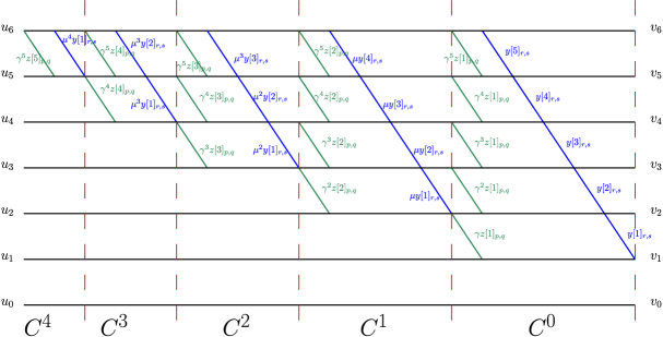
Figure 14. The planar network ${\mathcal{N}}_{7}$ up to source and sink vertices $u_{6}$ and $v_{6}$.

The first few rows of $\mathsf{F}(p,q,r,s,\gamma,\mu,y,z)$ are:

$$\left[\begin{array}[]{cccc}1&&&\\ 0&1&&\\ 0&\gamma z+y&1&\\ 0&\gamma^{2}pyz+\gamma^{3}pz^{2}+\gamma^{2}qyz+\gamma^{3}qz^{2}&\gamma^{2}pz+\gamma^{2}qz+\gamma^{2}z&1\\ &+\gamma^{2}yz+\gamma\mu yz+\mu y^{2}+ry^{2}+sy^{2}&+\mu y+ry+sy&\\ \vdots&\vdots&\vdots&\ddots\end{array}\right]$$ (6.80)

Clearly this matrix is coefficientwise totally positive jointly in $p,q,r,s,\gamma,\mu$, and the entries must count forests of trees on $n$ vertices with $k$ components with respect to eight different statistics. I present two main open problems regarding the matrix $\mathsf{F}(p,q,r,s,\gamma,\mu,y,z)$. The first is:

Problem 2.

Find a combinatorial interpretation of the entries of $\mathsf{F}(p,q,r,s,\gamma,\mu,y,z)$.

We know that specialising $p=r=y=z=1$ and $s=\gamma=\mu=q$ yields the $q$-forests matrix $\mathsf{F}(q)$, and the entries count forests on $n$ vertices with $k$ components according to the statistics presented in Section 3. Similarly, by specialising $\gamma=\mu=p=q=r=s=1$ we obtain the matrix $\mathsf{F}(y,z)$, the entries of which count $k$-component forests on $n$ vertices with respect to proper and improper edges. In the following subsections we identify other specialisations of $p,q,r,s,\gamma,\mu,y,z$ yielding matrices with entries that appear to count a variety of interesting combinatorial objects including: permutations with respect to left-right maxima, unordered forest of increasing labelled trees, $0$-$1$ tableaux by inversions and noninversions, and perfect matchings with respect to crossings and nestings.

Now define the row-generating polynomials of $\mathsf{F}(p,q,r,s,\gamma,\mu,y,z)$ to be

$$\mathsf{F}_{0}(x;p,q,r,s,\gamma,\mu,y,z)\;\coloneqq\;1$$ (6.81)

and

$$\mathsf{F}_{n}(x;p,q,r,s,\gamma,\mu,y,z)\;\coloneqq\;\sum_{l=0}^{n}f_{n,l}(p,q,r,s,\gamma,\mu,y,z)x^{l}$$ (6.82)

for $n>0$, and consider the Hankel matrix

$$H_{\infty}((\mathsf{F}_{n}(x;p,q,r,s,\gamma,\mu,y,z))_{n\geq 0})\coloneqq(\pi_{n,k})_{n,k\geq 0}$$ (6.83)

where

$$\pi_{n,k}\;=\;\mathsf{F}_{n+k}(x;p,q,r,s,\gamma,\mu,y,z).$$ (6.84)

The first few $\mathsf{F}_{n}(x;p,q,r,s,\gamma,\mu,y,z)$ are:

$$\begin{array}[]{c|c}n&\mathsf{F}_{n}(x;p,q,r,s,\gamma,\mu,y,z)\\ \hline\cr 0&1\\ 1&x\\ 2&x(x+y+\gamma z)\\ 3&x(x^{2}+(\mu+r+s)xy+(\mu+r+s)y^{2}+\gamma^{2}(1+p+q)xz\\ &+\gamma(\mu+\gamma(1+p+q))yz+\gamma^{3}(p+q)z^{2})\\ \vdots&\vdots\end{array}$$ (6.85)

so the associated Hankel matrix contains the $2\times 2$ minor:

$$\pi_{1,0}\pi_{2,1}-\pi_{2,0}\pi_{1,1}\;=\;\gamma^{2}px^{2}yz+\gamma^{3}px^{2}z^{2}+\gamma^{2}px^{3}z+\gamma^{2}qx^{2}yz+\gamma^{3}qx^{2}z^{2}+\gamma^{2}qx^{3}z\\ +\gamma^{2}x^{2}yz-\gamma^{2}x^{2}z^{2}+\gamma^{2}x^{3}z+\gamma\mu x^{2}yz-2\gamma x^{2}yz-2\gamma x^{3}z\\ +\mu x^{2}y^{2}+\mu x^{3}y+rx^{2}y^{2}+rx^{3}y+sx^{2}y^{2}+sx^{3}y-x^{2}y^{2}-2x^{3}y\not\succeq 0.$$ (6.86)

The polynomial sequence $(\mathsf{F}_{n}(x;p,q,r,s,\gamma,\mu,y,z))_{n\geq 0}$ is evidently not coefficientwise Hankel-totally positive. However, consider instead the matrix

$$\tilde{\mathsf{F}}(p,q,r,s,\gamma,\mu,y,z)\coloneqq(\tilde{f}_{n,k}(p,q,r,s,\gamma,\mu,y,z))_{n,k\geq 0}\\ \;=\;\mathsf{F}(p,q,r,s,\gamma,\mu,y,z)\mathop{\rm diag}\nolimits(((pqrs\gamma\mu)^{n(n-1)/2})_{n\geq 0}),$$ (6.87)

the row-generating polynomials of which are

$$\tilde{\mathsf{F}}_{0}(x;p,q,r,s,\gamma,\mu,y,z)\coloneqq 1$$ (6.88)

and

$$\tilde{\mathsf{F}}_{n}(x;p,q,r,s,\gamma,\mu,y,z)\coloneqq\sum_{k=0}^{n}\tilde{f}_{n,k}(p,q,r,s,\gamma,\mu)x^{k}$$ (6.89)

for $n>0$.

The sequence $(\tilde{\mathsf{F}}_{n}(x;p,q,r,s,\gamma,\mu,y,z))_{n\geq 0}$ is not coefficientwise Hankel-totally positive, however, my computations suggest that shifting the indeterminates $p,q,r,s,\gamma,\mu$ by $1$ yields a polynomial sequence that appears to be coefficientwise Hankel-totally positive jointly in nine indeterminates! I make the following conjecture:

Conjecture 6.7.

The polynomial sequence

$$(\tilde{\mathsf{F}}_{n}(x;1+p^{\prime},1+q^{\prime},1+r^{\prime},1+s^{\prime},1+\gamma^{\prime},1+\mu^{\prime},y,z))_{n\geq 0}$$ (6.90)

is coefficientwise Hankel-totally positive jointly in $x,y,z,p^{\prime},q^{\prime},r^{\prime},s^{\prime},\gamma^{\prime},\mu^{\prime}$.

I have verified the above conjecture to $5\times 5$, and I do not yet understand what these polynomials enumerate. The conjectured coefficientwise Hankel-total positivity of the shifted row-generating polynomials of $\tilde{\mathsf{F}}(p,q,r,s,\gamma,\mu,y,z)$ is in a sense stronger than the coefficientwise total positivity of $\tilde{\mathsf{F}}(p,q,r,s,\gamma,\mu,y,z)$ alone, and in light of this a combinatorial interpretation of the entries of $\tilde{\mathsf{F}}(p,q,r,s,\gamma,\mu,y,z)$ is much desired. Clearly each $(n,k)$-entry enumerates $k$-component forests on $n$ vertices with respect to eight statistics; interpreting these statistics is left as an open problem:

Problem 3.

Find a combinatorial interpretation of the entries of  $\tilde{\mathsf{F}}(p,q,r,s,\gamma,\mu,y,z)$.

6.4. $(p,q)$-Stirling polynomials

The network ${\mathcal{N}}_{7}$ is an interlacing of two different planar networks (one with green diagonal edges, one with blue). By setting $r=s=\mu=y=0$ we effectively remove the blue edges and are left with a binomial-like planar network we shall denote ${\mathcal{N}}_{7}^{\prime}$. Specialising $\gamma=z=1$ in ${\mathcal{N}}_{7}^{\prime}$ we obtain the binomial-like network with edge weights specialised to $\alpha_{i,l}=1$ and

$$\beta_{i,l}=[i-1]_{p,q},$$ (6.91)

with corresponding path matrix

$$G(p,q)\coloneqq(g_{n,k}(p,q))_{n,k\geq 0}\;=\;P_{{\mathcal{N}}_{7}^{\prime}}\;=\;\mathsf{F}(p,q,0,0,1,0,0,1)$$ (6.92)

The weights of the network ${\mathcal{N}}_{7}^{\prime}$ are purely $i$-dependent so the entries of $G(p,q)$ satisfy the recurrence:

$$g_{n,k}(p,q)\;=\;g_{n-1,k-1}(p,q)\;+\;[n-1]_{p,q}g_{n-1,k-1}(p,q)$$ (6.93)

for $n\geq 1$ with initial condition $g_{0,k}=\delta_{0k}$. Moreover we have

$$g_{n,k}(p,q)\;=\;{\mathbf{e}}_{n-k}([1]_{p,q},[2]_{p,q},\ldots,[n-1]_{p,q})$$ (6.94)

by way of (2.13) in Section 2. The recurrence (6.93) can be found in [17, Proposition 2.2] and [74], and the expression in terms of elementary functions (6.94) can be found in Proposition 2.3 (part (a)) of [17]. The entries of $G(p,q)$ are thus the $(p,q)$-Stirling cycle numbers (or unsigned $(p,q)$-Stirling numbers of the first kind, denoted $c_{p,q}[n,k]$) and the row-generating polynomials of $G(p,q)$ are

$$c_{n}(x;p,q)\coloneqq x\prod_{i=1}^{n-1}(x+y[i]_{p,q})$$ (6.95)

where $y=1$ (see Proposition 2.3 part (b) of [17]). Note that the authors of [17] have a combinatorial interpretation of $c_{p,q}[n,k]$, but it has nothing to do with forests and trees! Intead they consider $0$-$1$ tableaux: a $0$-$1$ tableau is a pair $\psi=(\lambda,f)$ where $\lambda=(\lambda_{1}\geq\lambda_{2}\geq\cdots\geq\lambda_{k})$ is a partition of an integer $m=|\lambda|$ and $f=(f_{i,j})_{1\leq j\leq\lambda_{i}}$ a filling of of the corresponding Ferrer’s diagram of $\lambda$ with $0$s and $1$s such that there is exactly one $1$ in each column. In [17] de Médicis and Leroux define two statistics on $\psi$: the inversion number, ${\rm inv}(\psi)$, is the number of $0$s below a $1$ in $\psi$, and the noninversion number, $\operatorname{nin}(\psi)$, is the number of $0$s above a $1$ in $\psi$. They then show that

$$c_{p,q}[n,k]\;=\;\sum_{\psi\in Td(n-1,n-k)}p^{\operatorname{nin}(\psi)}q^{{\rm inv}(\psi)}$$ (6.96)

where $Td(k,r)$ denotes the set of $0$-$1$ tableaux with $k$ rows and columns of length at most $r$, where the lengths of the columns are distinct.

Permutations, however, are perhaps arguably more natural objects to study in relation to generalisations of the Stirling cycle numbers (the polynomial $c_{n}(x;1,1)$ is the generating function for permutations counted with respect to cycles, after all). For $p$ specialised to $p=1$ Zeng [74, Section 3, where $s_{q}(n,k)=q^{n-k}c_{1,q}[n,k]$] showed that

$$c_{n}(x;1,q)\;=\;\sum_{\sigma\in\mathfrak{S}_{n}}x^{\textrm{lrm}(\sigma)}q^{{\rm inv}(\sigma)}$$ (6.97)

where lrm$(\sigma)$ denotes the number of left-right maxima in a permutation $\sigma$ (that is, the number of $\sigma(i)$ such $\sigma(i)>\sigma(j)$ for all $j<i$), and ${\rm inv}(\sigma)$ the number of inversions of $\sigma$ (that is, the number of pairs $i<j$ such that $\sigma(i)>\sigma(j)$), hence

$$g_{n,k}(1,q)\;=\;\sum_{\sigma\in\mathfrak{S}_{n}(k)}q^{{\rm inv}(\sigma)+k-n},$$ (6.98)

where $\mathfrak{S}_{n}(k)$ denotes the set of permutations on $[n]$ with $k$ left-right maxima.

Clearly $G(p,q)$ is totally positive, and for $p$ specialised to $p=1$ we can express the row-generating polynomials of $G(1,q)$ as the $S$-type (or Stieltjes-type) continued fraction

$$1+\sum_{n,k\geq 1}c_{1,q}[n,k]x^{k}t^{n}\;=\cfrac{1}{1-\cfrac{\lambda_{1}t}{1-\cfrac{\lambda_{2}t}{\cfrac{\cdots}{1-\cfrac{\lambda_{n}t}{\cdots}}}}}$$ (6.99)

where $\lambda_{2n-1}\coloneqq(x+[n]_{q})q^{n-1}$ and $\lambda_{2n}=[n]_{q}q^{n+1}$ for $n\geq 1$ (Lemma 3 of Zeng 1993, where we have replaced $x$ with $tq$, and $a$ with $x/q$). If a sequence of polynomials has an $S$-fraction with nonnegative coefficients then the corresponding Hankel matrix is coefficientwise totally positive (see [64] and [49, Section 9]), so we have:

Corollary 6.8.

The polynomial sequence $(c_{n}(x;1,q))_{n\geq 0}$ is coefficientwise Hankel-totally positive in $x,q$.

The Hankel matrix of $c_{n}(x;p,q)$, where $p$ and $q$ are indeterminates, however, begins

$$\left[\begin{array}[]{cccc}1&x&x(x+1)&\cdots\\ x&x(x+1)&x(x+1)(p+q+x)&\cdots\\ x(x+1)&x(x+1)(p+q+x)&x(x+1)(p+q+x)\left(p^{2}+pq+q^{2}+x\right)&\cdots\\ \vdots&\vdots&\vdots&\ddots\end{array}\right]$$ (6.100)

which contains the $2\times 2$ minor

$$\pi_{0,1}\pi_{1,2}-\pi_{1,1}\pi_{0,2}\;=\;px^{3}+px^{2}+qx^{3}+qx^{2}-x^{3}-x^{2}\not\succeq 0$$ (6.101)

so is not even TP₂ in ${\mathbb{Z}}[p,q]$. Again it appears, however, that right-multiplying $G(p,q)$ by a simple diagonal matrix yields a matrix whose row-generating polynomials appear to be coefficientwise Hankel-totally positive when $p,q$ are shifted by $1$.

Consider the matrix

$$G^{\prime}(p,q,\gamma,z)\;=\;(g^{\prime}_{n,k}(p,q,\gamma,z))_{n,k\geq 0}\;=\;\mathsf{F}(p,q,0,0,\gamma,0,0,z)\mathop{\rm diag}\nolimits(((pq\gamma)^{n(n-1)/2})_{n\geq 0})$$ (6.102)

and define its row-generating polynomials to be

$$G^{\prime}_{n}(x;p,q,\gamma,z)\coloneqq\sum_{k=0}^{n}g^{\prime}_{n,k}(p,q,\gamma,z)x^{k}.$$ (6.103)

Clearly $G^{\prime}(p,q,\gamma,z)$ is coefficientwise totally positive jointly in $p,q,\gamma,z$ (this follows from Cauchy-Binet and the LGV lemma). I make the following conjecture:

Conjecture 6.9.

The polynomial sequence $(G^{\prime}_{n}(x;p+1,q+1,\gamma+1,z))_{n\geq 0}$ is coefficientwise Hankel-totally positive jointly in $p,q,\gamma,z,x$.

I have verified this up to $7\times 7$, and am yet to discover a suitable combinatorial interpretation of these polynomials. I therefore pose the following problem:

Problem 4.

Find a combinatorial interpretation of the polynomials $G^{\prime}_{n}(x;p,q,\gamma,z)$.

6.5. Generalised Bessel polynomials

Now consider the planar network ${\mathcal{N}}_{7}^{\prime\prime}$ obtained by specialising $p=q=\gamma=z=0$ in ${\mathcal{N}}_{7}$ (effectively removing all diagonal blue edges from the network), and let

$$\mathsf{M}(r,s,\mu,y)\coloneqq(m_{n,k}(r,s,\mu,y))_{n,k\geq 0}\;=\;P_{{\mathcal{N}}_{7}^{\prime\prime}}\;=\;\mathsf{F}(0,0,r,s,0,\mu,y,0)$$ (6.104)

be the corresponding path matrix. The matrix $\mathsf{M}(r,s,\mu,y)$ has a factorisation in terms of downshifted inverse bidiagonal matrices:

$$\mathsf{M}(r,s,\mu,y)\;=\;\cdots\left[\begin{array}[]{c|c}I_{3}&0\\ \hline\cr 0&T({\mathbf{a}}_{2}(r,s,\mu,y))\end{array}\right]\cdot\left[\begin{array}[]{c|c}I_{2}&0\\ \hline\cr 0&T({\mathbf{a}}_{1}(r,s,\mu,y))\end{array}\right]\cdot\left[\begin{array}[]{c|c}1&0\\ \hline\cr 0&T({\mathbf{a}}_{0}(r,s,\mu,y))\end{array}\right]$$ (6.105)

where ${\mathbf{a}}_{i}(r,s,\mu,y)=(\mu^{i}y[n+1]_{r,s})_{n\geq 0}$.

Each matrix $T({\mathbf{a}}_{i}(r,s,\mu,y))$ has $(n,k)$-entry:

$$\mu^{i(n-k)}y\frac{[n]_{r,s}!}{[k]_{r,s}!}$$ (6.106)

and specialising $r,s,\mu$ to $r=s=\mu=1$ we obtain

$$\left[\begin{array}[]{c|c}1&0\\ \hline\cr 0&T({\mathbf{a}}_{i}(1,1,1,y))\end{array}\right]\;=\;\left[\begin{array}[]{ccccccc}1&&&&&&\\ 0&1&&&&&\\ 0&y&1&&&&\\ 0&2y^{2}&2y&1&&&\\ 0&6y^{3}&6y^{2}&3y&1&&\\ 0&24y^{4}&24y^{3}&12y^{2}&4y&1&\\ \vdots&\vdots&\vdots&\vdots&\vdots&\vdots&\ddots\end{array}\right]$$ (6.107)

(this array appears in [63, A094587]). Compare the above with the production matrix $\mathsf{P}_{\boldsymbol{\phi}}\coloneqq(p_{n,k})_{n,k\geq 0}$ defined in Proposition 1.4 of [48], where

$$p_{n,k}\;=\;\begin{cases}0&\textrm{if }k=0,\\ \displaystyle\frac{n!}{(k-1)!}\phi_{n-k+1}&\textrm{if }n\geq k-1.\end{cases}$$ (6.108)

We have

$$\mathsf{P}_{\boldsymbol{\phi}}\;=\;\left[\begin{array}[]{ccccccc}0&1&&&&&\\ 0&\phi_{1}&1&&&&\\ 0&2\phi_{2}&2\phi_{1}&1&&&\\ 0&6\phi_{3}&6\phi_{2}&3\phi_{1}&1&&\\ 0&24\phi_{4}&24\phi_{3}&12\phi_{2}&4\phi_{1}&1&\\ \vdots&\vdots&\vdots&\vdots&\vdots&\vdots&\ddots\end{array}\right],$$ (6.109)

(where $\boldsymbol{\phi}=(\phi_{n})_{n\geq 0}$ is a sequence of indeterminates, and for ease of reading we set $\phi_{0}=1$). It is easy to see that (6.107) is the augmented production matrix obtained by setting $\phi_{i}=y^{i}$ in $\mathsf{P}_{\boldsymbol{\phi}}$.

The output matrix of $\mathsf{P}_{\boldsymbol{\phi}}$ is the generic Lah triangle:

$$\mathsf{L}\coloneqq(L_{n,k}(\boldsymbol{\phi}))_{n,k\geq 0}\;=\;\left[\begin{array}[]{ccccccc}1&&&&&&\\ 0&1&&&&\\ 0&\phi_{1}&1&&&\\ 0&\phi_{1}^{2}+2\phi_{2}&3\phi_{1}&1&&\\ 0&\phi_{1}^{3}+8\phi_{1}\phi_{2}+6\phi_{3}&7\phi_{1}^{2}+8\phi_{2}&6\phi_{1}&1&\\ \vdots&\vdots&\vdots&\vdots&\vdots&\ddots\end{array}\right],$$ (6.110)

the row-generating polynomials of which are

$$L_{n}(\boldsymbol{\phi},y)\coloneqq\sum_{k=0}^{n}L_{n,k}(\boldsymbol{\phi})y^{k}.$$ (6.111)

The entries of $\mathsf{L}$ are generating polynomials for unordered forests of increasing ordered trees on the vertex set $[n]$ having $k$ components, in which each vertex with $i$ children is assigned a weight $\phi_{i}$. Setting $\boldsymbol{\phi}=(1)_{n\geq 0}$ in (6.110) we obtain the reverse Bessel triangle:

$$\mathsf{M}(1,1,1,1)\;=\;\left[\begin{array}[]{ccccccc}1&&&&&&\\ 0&1&&&&&\\ 0&1&1&&&&\\ 0&3&3&1&&&\\ 0&15&15&6&1&&\\ 0&105&105&45&10&1&\\ \vdots&\vdots&\vdots&\vdots&\vdots&\vdots&\ddots\end{array}\right]$$ (6.112)

(see [63, A001497]). The row-generating polynomials of $\mathsf{M}(1,1,1,1)$ are the reverse Bessel polynomials (see [33])

$$\theta_{n}(x)\;\coloneqq\;\sum_{k=0}^{n}\frac{(n+k)!}{(n-k)!k!}\left(\frac{x^{n-k}}{2^{k}}\right),$$ (6.113)

which is an orthogonal sequence of polynomials related to the Bessel polynomials (see [44, 33]):

$$y_{n}(x)\coloneqq\sum_{k=0}^{n}\frac{(n+k)!}{(n-k)!k!}\left(\frac{x}{2}\right)^{k}$$ (6.114)

via the identity

$$\theta_{n}(x)\;=\;x^{n}y_{n}(1/x).$$ (6.115)

It follows from [48] that the sequence of polynomials $\theta_{n}(x)$ is coefficientwise Hankel-totally positive.

Consider now the row-generating polynomials of $\mathsf{M}(r,s,\mu,y)$, defined to be

$$\mathsf{M}_{0}(x;r,s,\mu,y)\;\coloneqq\;1$$ (6.116)

and

$$\mathsf{M}_{n}(x;r,s,\mu,y)\coloneqq\sum_{k=0}^{n}m_{n,k}(r,s,\mu,y)x^{k}$$ (6.117)

for $n>0$, and note that the polynomials $\mathsf{M}_{n}(x;r,s,\mu,y)$ are generalisations of the reverse Bessel polynomials in the sense that $\mathsf{M}_{n}(x;1,1,1,1)=\theta_{n}(x)$.

It follows from [48] that the polynomial sequence $(\mathsf{M}_{n}(x;1,1,1,y))_{n\geq 0}$ is coefficientwise totally positive jointly in $x$ and $y$. Again, it is natural to ask whether the generalisation where $r,s,\mu,y$ are left as indeterminates preserves coefficientwise Hankel-totally positivity. The answer is no, since the Hankel matrix

$$H_{\infty}((\mathsf{M}_{n}(x;r,s,\mu,y))_{n\geq 0})\;=\;(\pi_{n,k})_{n,k\geq 0},$$ (6.118)

where

$$\pi_{n,k}\;=\;\mathsf{M}_{n+k}(x;r,s,\mu,y)$$ (6.119)

contains the $2\times 2$ minor

$$\pi_{1,0}\pi_{2,1}-\pi_{2,0}\pi_{1,1}\;=\;\mu x^{2}y^{2}+\mu x^{3}y+rx^{2}y^{2}+rx^{3}y+sx^{2}y^{2}+sx^{3}y-x^{2}y^{2}-2x^{3}y\not\succeq 0.$$ (6.120)

Once more, however, it appears that Hankel-total positivity could well be restored by right-multiplying $\mathsf{M}(r,s,\mu,y)$ by a simple diagonal matrix and shifting $r,s,\mu$ by $1$.

Consider the matrix

$$\mathsf{M}^{\prime}(r,s,\mu,y)\coloneqq(m^{\prime}_{n,k}(r,s,\mu,y))_{n,k\geq 0}\;=\;\mathsf{M}(r,s,\mu,y)\mathop{\rm diag}\nolimits(((rs\mu)^{n(n-1)/2})_{n\geq 0})$$ (6.121)

and let

$$\mathsf{M}^{\prime}_{0}(x;r,s,\mu,y)\coloneqq 1$$ (6.122)

and

$$\mathsf{M}^{\prime}_{n}(x;r,s,\mu,y)\coloneqq\sum_{k=0}^{n}m^{\prime}_{n,k}(r,s,\mu,y)x^{k}$$ (6.123)

for $n>0$ be the corresponding row-generating polynomials of $\mathsf{M}^{\prime}(r,s,\mu,y)$. I conjecture:

Conjecture 6.10.

The sequence of polynomials $(\mathsf{M}^{\prime}_{n}(x;r+1,s+1,\mu+1,y))_{n\geq 0}$ is coefficientwise Hankel-totally positive jointly in $r,s,\mu,x,y$.

I have verified this up to $5\times 5$, and am yet to discover a suitable combinatorial interpretation of the entries of $\mathsf{M}(r,s,\mu,y)$ or indeed $\mathsf{M}^{\prime}(r,s,\mu,y)$, and therefore pose the following problem:

Problem 5.

Find combinatorial interpretations of $\mathsf{M}^{\prime}(r,s,\mu,y)$ and $\mathsf{M}(r,s,\mu,y)$.

There is one final observation to make concerning perfect matchings that may help in tackling the foregoing problem. A perfect matching $M$ on $[2n]$ is a partition of $1,2,\ldots,2n$ into $n$ pairs $(i,j)$ where $i<j$. We denote the set of all such perfect matchings ${\mathcal{M}}_{2n}$, and it is well-known that

$$|{\mathcal{M}}_{2n}|\;=\;(2n-1)!!.$$ (6.124)

Two pairs $(i_{r},j_{r})$ and $(i_{s},j_{s})$ belonging to $M\in{\mathcal{M}}_{2n}$ form a crossing if $i_{r}<i_{s}<j_{r}<j_{s}$, and form a nesting if $i_{r}<i_{s}<j_{s}<j_{r}$. The number of crossings in $M$ is denoted ${\rm cr}(M)$ and the number of nestings is denoted ${\rm ne}(M)$.

If $\mu$ and $y$ are specialised to $\mu=y=1$ then the first few rows of $\mathsf{M}(r,s,1,1)$ are:

$${\small\left[\begin{array}[]{cccccc}1&&&&&\\ 0&1&&&&\\ 0&1&1&&&\\ 0&r+s+1&r+s+1&1&&\\ 0&2r^{2}s+r^{3}+r^{2}+2rs^{2}+2rs\hfill&2r^{2}s+r^{3}+r^{2}+2rs^{2}+2rs\hfill&r^{2}+rs+r\hfill&1&\\ &\hfill+2r+s^{3}+s^{2}+2s+1&\hfill+2r+s^{3}+s^{2}+2s+1&\hfill+s^{2}+s+1&&\\ \vdots&\vdots&\vdots&\vdots&\vdots&\ddots\\ \end{array}\right]}.$$ (6.125)

For $s$ specialised to $s=1$ and $0<n\leq 20$ I have verified empirically that

$$m_{n,1}(r,1,1,1)\;=\;(1-r)^{1-n}\sum_{k=0}^{n-1}(-1)^{k}r^{k(k+1)/2}\frac{2k+1}{2n-1}\binom{2n-1}{n+k}.$$ (6.126)

The formula above (where $n$ is replaced with $n+1$) was found implicitly by Touchard [73], and explicitly by Riordan [58] (see also [4, 41, 47, 53, 56]), and counts perfect matchings with respect to crossings (or nestings):

$$\sum_{M\in{\mathcal{M}}_{2n}}r^{{\rm cr}({\mathcal{M}})}\;=\;\sum_{M\in{\mathcal{M}}_{2n}}r^{{\rm ne}({\mathcal{M}})}\;=\;(1-r)^{-n}\sum_{k=0}^{n}(-1)^{k}r^{k(k+1)/2}\frac{2k+1}{2n+1}\binom{2n+1}{n+k+1}.$$ (6.127)

However, more may indeed be true, since it looks like the $k=1$ column of $\mathsf{M}(r,s,1,1)$ counts perfect matchings with respect to crossings and nestings. For $0<n\leq 20$ my computations have confirmed that

$$m_{n,1}(r,s,1,1)\;=\;[t^{n}]S(t;r,s)$$ (6.128)

where $S(t;r,s)$ is the $S$-type continued fraction

$$S(t;r,s)\coloneqq\cfrac{1}{1-\cfrac{[1]_{r,s}t}{1-\cfrac{[2]_{r,s}t}{\cfrac{\cdots}{1-\cfrac{[n]_{r,s}t}{\cdots}}}}}.$$ (6.129)

Since $S(t;r,s)$ is the master $S$-fraction for perfect matchings first given by Kasraoui and Zeng in [43, Proposition 4.4, with $p,q$ replaced by $r,s$ respectively] (see also [68, Theorem 4.4] specialised to $x=y=u=v=1$, $p_{+}=p_{-}=r$, and $q_{+}=q_{-}=s$), I make the following conjecture:

Conjecture 6.11.

For $n>1$

$$m_{n,1}(r,s,1,1)\;=\;\sum_{M\in{\mathcal{M}}_{2(n-1)}}r^{{\rm cr}(M)}s^{{\rm ne}(M)}.$$ (6.130)

As described above, there exists an explicit formula for counting perfect matchings with respect to crossings or nestings given by Touchard and Riordan, however, an explicit closed formula that counts perfect matchings with respect to crossings and nestings is yet to be found. I therefore pose the following problem:

Problem 6.

Find a closed form formula for $m_{n,1}(x;r,s,1,1)$.

References

- [1] M. Aigner and G. M. Ziegler, Proofs from The Book, 6th ed., Springer-Verlag, Berlin, 2018.
- [2] G. E. Andrews, The Theory of Partitions, Encyclopedia of Mathematics and its Applications, Cambridge University Press, 1984.
- [3] A. Avro and N. Dershowitz, Cayley’s formula: A page from The Book, The American Mathematical Monthly 123 (2016), no. 7, pp. 699 – 700.
- [4] N. Blitvić, The -Gaussian process, J. Funct. Anal. 263 (2012), pp. 3270 – 3305.
- [5] F. Brenti, Combinatorics and total positivity, J. Combin. Theory A 71 (1995), pp. 175 – 218.
- [6] by same author, The applications of total positivity to combinatorics, and conversely., Total Positivity and its Applications (M. Gasca and C. A. Micchelli, eds.), Kluwer, Dordrecht, 1996, pp. 451 – 473.
- [7] C. Chauve, S. Dulucq, and O. Guibert, Enumeration of some labelled trees, Research Report RR-1226-99 (1999), LaBRI, Universite Bordeaux I.
- [8] by same author, Enumeration of some labelled trees, Formal Power Series and Algebraic Combinatorics (FPSAC 2000), Springer-Verlag, Berlin, 2000, pp. 146 – 157.
- [9] W. Y. C. Chen and H. R. L. Yang, A context-free grammar for the Ramanujan–-Shor polynomials, Adv. Appl. Math. 126 (2021), no. 101908, p. 24.
- [10] Xi. Chen, B. Deb, A. Dyachenko, T. Gilmore, and A. D. Sokal, Coefficientwise total positivity of some matrices defined by linear recurrences, in preparation.
- [11] by same author, Coefficientwise total positivity of some matrices defined by linear recurrences, (2020), to appear in the proceedings of FPSAC 2021.
- [12] G.-S. Cheon, J.-H. Jung, and Y. Lim, A -analogue of the Riordan group, Linear Algebra and its Applications 439 (2013), no. 12, pp. 4119 – 4129.
- [13] J. Cigler, -Abel polynomials, (2008), arXiv:0802.2886.
- [14] L. E. Clarke, On Cayley’s Formula for Counting Trees, Journal of the London Mathematical Society 1-33 (1958), no. 4, pp. 471–474.
- [15] L. Comtet, Advanced Combinatorics: The Art of Finite and Infinite expansions, Reidel, Dordrecht–Boston, 1974, translated from the French by J.W. Nienhuys. [French original: Analyse Combinatoire, tomes I et II, Presses Universitaires de France, Paris, 1970.].
- [16] R. M. Corless, G. H. Gonnet, D. E. G. Hare, D. J. Jeffrey, and D. E. Knuth, On the Lambert W function, Advances in Computational Mathematics 5 (1996), no. 1, pp. 329 – 359.
- [17] A. de Médicis and P. Leroux, A unified combinatorial approach for - (and -) Stirling numbers, Journal of Statistical Planning and Inference 34 (1993), no. 1, pp. 89 – 105.
- [18] E. Deutsch, L. Ferrari, and S. Rinaldi, Production Matrices and Riordan Arrays, Annals of Combinatorics 13 (2009), no. 1, pp. 65 – 85.
- [19] E. Deutsch and L. Shapiro, Exponential Riordan arrays, handwritten lecture notes, Nankai University, available online at http://www.combinatorics.net/ppt2004/Louis%20W.%20Shapiro/shapiro.pdf, 26 February 2004.
- [20] D. Dumont and A. Ramamonjiosa, Grammaire de Ramanujan et arbres de Cayley, Electron. J. Combin. 3 (1996), no. R17.
- [21] Ö. Eǧecioǧlu and J. B. Remmel, Bijections for Cayley trees, spanning trees, and their -analogues, J. Combin. Theory A 42 (1986), no. 1, pp. 15 – 30.
- [22] S. M. Fallat and C. R. Johnson, Totally Nonnegative Matrices, Princeton University Press, Princeton NJ, 2011.
- [23] F. Flajolet, Combinatorial aspects of continued fractions, Discrete Math. (1980), pp. 125 – 161.
- [24] S. Fomin and A. Zelevinsky, Total positivity: tests and parametrizations, Math. Intelligencer 22 (2000), pp. 23 – 33.
- [25] Jean Françon, Preuves combinatoires des identites d’Abel, Discrete Mathematics 8 (1974), no. 4, pp. 331 – 343.
- [26] F. R. Gantmacher and M. G. Krein, Oscillation Matrices and Kernels and Small Vibrations of Mechanical Systems, AMS Chelsea Publishing, Providence RI, 2002, based on the second Russian edition, 1950.
- [27] G. Gasca and G. Mühlbach, A test for strict total positivity via Neville elimination, Current Trends in Matrix Theory (F. Uhlig and R. Groue, eds.), Elsevier Science, 1987, pp. 225 – 232.
- [28] M. Gasca and E. Lebròn, Elimination techniques and interpolation, J. Comput. Appl. Math. 19 (1987), pp. 125 – 132.
- [29] M. Gasca and G. Mühlbach, Generalized Schur complements and a test for total positivity, Appl. Numer. Math. 3 (1987), pp. 215 – 232.
- [30] M. Gasca and J. M. Peña, Total positivity and Neville elimination, Linear Algebra and its Applications 165 (1992), pp. 25 – 44.
- [31] I. M Gessel and S. Seo, A refinement of Cayley’s formula for trees, Elec. J. Combin. 11 (2006), no. R.27.
- [32] Ira M. Gessel, A q-analog of the exponential formula, Discrete Mathematics 306 (2006), no. 10, pp. 1022 – 1031, 35th Special Anniversary Issue.
- [33] E. Grosswald, Bessel Polynomials, Lecture Notes Math. 698 (1978).
- [34] S. Guo and J. W. Guo, A recursive algorithm for trees and forests, Discrete Mathematics 340 (2017), no. 4, pp. 695 – 703.
- [35] V. J. W. Guo, A bijective proof of the Shor recurrence, European J. Combin. 70 (2018), pp. 92 – 98.
- [36] V. J. W. Guo and J. Zeng, A generalization of the Ramanujan polynomials and plane trees, Avd. Appl. Math. 39 (2007), pp. 96 – 115.
- [37] F. H. Jackson, A -generalization of Abel’s series, Rendiconti Palermo 29 (1910), pp. 340 – 346.
- [38] W. P. Johnson, -extensions of identities of Abel-Rothe type, Discrete Mathematics 159 (1996), no. 1, pp. 161 – 177.
- [39] Warren P. Johnson, Some applications of the q-exponential formula, Discrete Mathematics 157 (1996), no. 1, pp. 207 – 225.
- [40] M. Josuat-Vergès, Derivatives of the tree function, Ramanujan J. 38 (2015), pp. 1 – 15.
- [41] M. Josuat-Vergès and J. S. Kim, Touchard–-Riordan formulas, T–fractions, and Jacobi’s triple product identity, Ramanujan J. 30 (2013), pp. 341 – 378.
- [42] S. Karlin, Total Positivity, Stanford University Press, Stanford CA, 1968.
- [43] A. Kasraoui and J. Zeng, Distribution of crossings, nestings and alignments of two edges in matchings and partitions, Elec. J. Comb. 13 (2006), no. 1.
- [44] H. L. Krall and O. Frink, A new class of orthogonal polynomials: The Bessel polynomials, Trans. Amer. Math. Soc. 63 (1949), pp. 100 – 115.
- [45] Z. Lin and J. Zeng, Positivity properties of Jacobi–Stirling numbers and generalized Ramanujan polynomials, Adv. Appl. Math 53 (2014), pp. 12 – 27.
- [46] J. W. Moon, Counting labelled trees, Canadian Mathematical Congress, Montreal, 1970.
- [47] J.-G. Penaud, Une preuve bijective d’une formule de Touchard–-Riordan, Discrete Math. 139 (1995), pp. 347 – 360.
- [48] M. Pétréolle and A. D. Sokal, Lattice paths and branched continued fractions ii. Multivariate Lah polynomials and Lah symmetric functions, European Journal of Combinatorics 92 (2021), pp. 103 – 235.
- [49] M. Pétréolle, A. D. Sokal, and B. Zhu, Lattice paths and branched continued fractions: An infinite sequence of generalizations of the Stieltjes–Rogers and Thron–Rogers polynomials, with coefficientwise Hankel-total positivity, (2020), accepted for publications in Memoirs of the AMS.
- [50] J. F. Pfaff, Allgemeine Summation einer Reihe, worinn höhere differenziale vorkommen, Archiv der reinen und angewandten Mathematik 1 (1795), pp. 337 – 347.
- [51] A. Pinkus, Totally Positive Matrices, Cambridge University Press, Cambridge, 2010.
- [52] J. Pitman, Forest Volume Decompositions and Abel–-Cayley-–Hurwitz Multinomial Expansions, J. Combin. Theory, Series A 98 (2002), no. 1, pp. 175 – 191.
- [53] H. Prodinger, On Touchard’s continued fraction and extensions: combinatorics-free, self-contained proofs, Quaestiones Math. 35 (2012), pp. 431 – 445.
- [54] H. Prüfer, Neuer Beweis eines Satzes über Permutationen, Arch. Math. Phys. 27 (1918), pp. 742 – 744.
- [55] L. Randazzo, Arboretum for a generalisation of Ramanujan polynomials, Ramanujan J. 54 (2021), pp. 591 – 604.
- [56] R. C. Read, The chord intersection problem, Second International conference on Combinatorial Mathematics: Annals of the New York Academy of Sciences No. 319 (A. Gerwitz and L. V Quintas, eds.), New York Academy of Sciences, New York, 1979, pp. pp. 444 – 454.
- [57] J. Riordan, Forests of labeled trees, J. Combin. Theory 5 (1968), pp. 90 – 103.
- [58] by same author, The distribution of crossings of chords joining pairs of points on a circle, Math. Comp. 29 (1975), pp. 215 – 222.
- [59] H. A. Rothe, Formulae de serierum reversione demonstratio universalis signislocalibus combinatorioanalyticorum vicariis exhibita, Litteris Sommeriis, Leipzig, 1793.
- [60] Bruce E. Sagan, A note on Abel polynomials and rooted labeled forests, Discrete Mathematics 44 (1983), no. 3, pp. 293 – 298.
- [61] L. Schläfli, Bemerkungen über die Lambertische Reihe, Archiv der Mathematikund Physik 10 (1847), pp. 332 –– 340, Reprinted in L. Schläfli, Gesammelte Mathematische Abhandlungen, Band I (Springer, Basel, 1950), pp. 38–45.
- [62] P. W. Shor, A new proof of Cayley’s formula for counting labeled trees, J. Combin. Theory A 71 (1995), pp. 154 – 158.
- [63] N. Sloane, The Online Encyclopedia of Integer Sequences, available at http://oeis.org.
- [64] A. D. Sokal, Coefficientwise total positivity (via continued fractions) for some hankel matrices of combinatorial polynomials, in preparation.
- [65] by same author, A remark on the enumeration of rooted labeled trees, Discrete Mathematics 343 (2020), no. 7.
- [66] A. D. Sokal, Total Positivity of some polynomial matrices that enumerate labelled trees and forests: I. Forests of rooted labelled trees, (2021), arXiv:2105.05583.
- [67] A. D. Sokal and X. Chen, Total positivity of some polynomial matrices that enumerate labelled trees and forests: II. Rooted labelled trees, (2021), in preparation.
- [68] A. D. Sokal and J. Zeng, Some multivariate master polynomials for permutations, set partitions, and perfect matchings, and their continued fractions, 2020, arXiv:2003.08192.
- [69] R. P. Stanley, Enumerative Combinatorics, vol. 2, Wadsworth & Brooks/Cole, Monterey CA, 1986, reprinted by Cambridge University Press, 1999.
- [70] T. J. Stieltjes, Recherches sur les fractions continues, Ann. Fac. Sci. Toulouse 8 (1894), no. J1 – J122.
- [71] by same author, Recherches sur les fractions continues, Ann. Fac. Sci. Toulouse 9 (1895), no. A1 – A47.
- [72] by same author, Euvres Complète/Collected Papers, vol. II, Springer-Verlag, Berlin, 1993.
- [73] J. Touchard, Sur un problème de configurations et sur les fractions continues, Canad. J. Math 4 (1952), pp. 2 – 25.
- [74] J. Zeng, The -Stirling numbers, continued fractions and the -Charlier and -Laguerre polynomials, Journal of Computational and Applied Mathematics 57 (1995), no. 3, pp. 413 – 424.
- [75] by same author, A Ramanujan sequence that refines the Cayley formula for trees, Ramanujan J. 3 (1999), pp. 45 – 54.