SpanNer: Named Entity Re-/Recognition as Span Prediction

Abstract

Recent years have seen the paradigm shift of Named Entity Recognition (NER) systems from sequence labeling to span prediction. Despite its preliminary effectiveness, the span prediction model’s architectural bias has not been fully understood. In this paper, we first investigate the strengths and weaknesses when the span prediction model is used for named entity recognition compared with the sequence labeling framework and how to further improve it, which motivates us to make complementary advantages of systems based on different paradigms. We then reveal that span prediction, simultaneously, can serve as a system combiner to re-recognize named entities from different systems’ outputs. We experimentally implement 154 systems on 11 datasets, covering three languages, comprehensive results show the effectiveness of span prediction models that both serve as base NER systems and system combiners. We make all code and datasets available: https://github.com/neulab/spanner, as well as an online system demo: http://spanner.sh. Our model also has been deployed into the ExplainaBoard Liu et al. (2021) platform, which allows users to flexibly perform the system combination of top-scoring systems in an interactive way: http://explainaboard.nlpedia.ai/leaderboard/task-ner/.

1 Introduction

The rapid evolution of neural architectures Kalchbrenner et al. (2014a); Kim (2014); Hochreiter and Schmidhuber (1997) and large pre-trained models Devlin et al. (2019); Lewis et al. (2020) not only drive the state-of-the-art performance of many NLP tasks Devlin et al. (2019); Liu and Lapata (2019) to a new level but also change the way how researchers formulate the task. For example, recent years have seen frequent paradigm shifts for the task of named entity recognition (NER) from token-level tagging, which conceptualize NER as a sequence labeling (SeqLab) task Chiu and Nichols (2015); Huang et al. (2015); Ma and Hovy (2016); Lample et al. (2016); Akbik et al. (2018); Peters et al. (2018); Devlin et al. (2018); Xia et al. (2019); Luo et al. (2020); Lin et al. (2020); Fu et al. (2021), to span-level prediction (SpanNer) Li et al. (2020); Mengge et al. (2020); Jiang et al. (2020); Ouchi et al. (2020); Yu et al. (2020), which regards NER either as question answering Li et al. (2020); Mengge et al. (2020), span classification Jiang et al. (2020); Ouchi et al. (2020); Yamada et al. (2020), and dependency parsing tasks Yu et al. (2020).

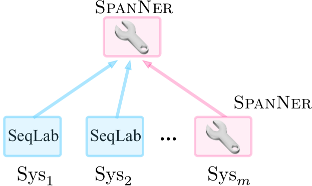
Figure 1: ONE span prediction model (SpanNER) finishes TWO things: (1) named entity recognition (2) combination of different NER systems.

However, despite the success of span prediction-based systems, as a relatively newly-explored framework, the understanding of its architectural bias has not been fully understood so far. For example, what are the complementary advantages compared with SeqLab frameworks and how to make full use of them? Motivated by this, in this paper, we make two scientific contributions.

We first investigate what strengths and weaknesses are when NER is conceptualized as a span prediction task. To achieve this goal, we perform a fine-grained evaluation of SpanNer systems against SeqLab systems and find there are clear complementary advantages between these two frameworks. For example, SeqLab-based models are better at dealing with those entities that are long and with low label consistency. By contrast, SpanNer systems do better in sentences with more Out-of-Vocabulary (OOV) words and entities with medium length (§3.3).

Secondly, we reveal the unique advantage brought by the architectural bias of the span prediction framework: it can not only be used as a base system for named entity recognition but also serve as a meta-system to combine multiple NER systems’ outputs. In other words, the span prediction model play two roles showing in Fig. 1: (i) as a base NER system; and (ii) as a system combiner of multiple base systems. We claim that compared with traditional ensemble learning of the NER task, SpanNer combiners are advantageous in the following aspects:

1. Most of the existing NER combiners rely on heavy feature engineering and external knowledge Florian et al. (2003); Wu et al. (2003); Saha and Ekbal (2013). Instead, the SpanNer models we proposed for system combination train in an end-to-end fashion.

2. Combining complementarities of different paradigms: most previous works perform NER system combination solely focusing on the sequence labeling framework. It is still an understudied topic how systems from different frameworks help each other.

3. No extra training overhead and flexibility of use: Existing ensemble learning algorithms are expensive, which usually need to collect training samples by k-fold cross-validation for system combiner Speck and Ngomo (2014), reducing their practicality.

4. Connecting two separated training processes: previously, the optimization of base NER systems and ensemble learning for combiner are two independent processes. Our work builds their connection and the same set of parameters shared over these two processes.

Experimentally, we first implement 154 systems on 11 datasets, on which we comprehensively evaluate the effectiveness of our proposed span prediction-based system combiner. Empirical results show its superior performance against several typical ensemble learning algorithms.

Lastly, we make an engineering contribution that benefits from the practicality of our proposed methods. Specifically, we developed an online demo system based on our proposed method, and integrate it into the NER Leaderboard, which is very convenient for researchers to find the complementarities among different combinations of systems, and search for a new state-of-the-art system.

2 Preliminaries

2.1 Task

NER is frequently formulated as a sequence labeling (SeqLab) problem (Chiu and Nichols, 2015; Huang et al., 2015; Ma and Hovy, 2016; Lample et al., 2016), where $X=\{x_{1},x_{2},\ldots,x_{T}\}$ is an input sequence and $Y=\{y_{1},y_{2},\ldots,y_{T}\}$ is the output label (e.g., “B-PER”, “I-LOC”, “O”) sequence. The goal of this task is to accurately predict entities by assigning output label $y_{t}$ for each token $x_{t}$. We take the F1-score as the evaluation metric for the NER task.

2.2 Datasets

To make a comprehensive evaluation, in this paper, we use multiple NER datasets that cover different domains and languages.

CoNLL-2003 (Sang and De Meulder, 2003) covers two different languages: English and German. Here, we only consider the English (EN) dataset collected from the Reuters Corpus.

CoNLL-2002 (Sang, 2002) contains annotated corpus in Dutch (NL) collected from De Morgen news, and Spanish (ES) collected from Spanish EFE News Agency. We evaluate both languages.

OntoNotes 5.0 (Weischedel et al., 2013) is a large corpus consisting of three different languages: English, Chinese, and Arabic, involving six genres: newswire (NW), broadcast news (BN), broadcast conversation (BC), magazine (MZ), web data (WB), and telephone conversation (TC). Following previous works Durrett and Klein (2014); Ghaddar and Langlais (2018), we utilize different domains in English to test the robustness of proposed models.

WNUT-2016 and WNUT-2017 (Strauss et al., 2016; Derczynski et al., 2017) are social media data from Twitter, which were public as a shared task at WNUT-2016 (W16) and WNUT-2017 (W17).

3 Span Prediction for NE Recognition

Although this is not the first work that formulates NER as a span prediction problem Jiang et al. (2020); Ouchi et al. (2020); Yu et al. (2020); Li et al. (2020); Mengge et al. (2020), we contribute by (1) exploring how different design choices influence the performance of SpanNer and (2) interpreting complementary strengths between SeqLab and SpanNer with different design choices. In what follows, we first detail span prediction-based NER systems with the vanilla configuration and proposed advanced featurization.

3.1 SpanNer as NER System

Overall, the span prediction-based framework for NER consists of three major modules: token representation layer, span representation layer, and span prediction layer.

3.1.1 Token Representation Layer

Given a sentence $X=\{x_{1},\cdots,x_{n}\}$ with $n$ tokens, the token representation $\mathbf{h}_{i}$ is as follows:

$$\mathbf{u}_{1},\cdots,\mathbf{u}_{n} =\textsc{Emb}(x_{1},\cdots,x_{n}),$$ (1)

$$\mathbf{h}_{1},\cdots,\mathbf{h}_{n} =\textsc{BiLSTM}(\mathbf{u}_{1},\cdots,\mathbf{u}_{n}),$$ (2)

where $\textsc{Emb}(\cdot)$ is the pre-trained embeddings, such as non-contextualized embeddings GloVe (Pennington et al., 2014) or contextualized pre-trained embeddings BERT (Devlin et al., 2018). BiLSTM is the bidirectional LSTM Hochreiter and Schmidhuber (1997).

3.1.2 Span Representation Layer

First, we enumerate all the possible $m$ spans $S=\{s_{1},\cdots,s_{i},\cdots,s_{m}\}$ for sentence $X=\{x_{1},\cdots,x_{n}\}$ and then re-assign a label $y\in\mathcal{Y}$ for each span $s$. For example, for sentence: “London₁ is₂ beautiful₃”, the possible span’s (start, end) indices are $\{(1,1),(2,2),(3,3),(1,2),(2,3),(1,3)\}$, and the labels of these spans are all “O” except $(1,1)$ (London) is “LOC”. We use $b_{i}$ and $e_{i}$ to denote the start- and end- index of the span $s_{i}$, respectively, and $1\leq b_{i}\leq e_{i}\leq n$. Then each span can be represented as $s_{i}=\{x_{b_{i}},x_{b_{i}+1},\cdots,x_{e_{i}}\}$. The vectorial representation of each span could be calculated based on the following parts:

Boundary embedding: span representation is calculated by the concatenation of the start and end tokens’ representations $\mathbf{z}_{i}^{b}=[\mathbf{h}_{b_{i}};\mathbf{h}_{e_{i}}]$

Span length embedding: we additionally featurize each span representation by introducing its length embedding $\mathbf{z}_{i}^{l}$, which can be obtained by a learnable look-up table.

The final representation of each span $s_{i}$ can be obtained as: $\mathbf{s}_{i}=[\mathbf{z}_{i}^{b};\mathbf{z}_{i}^{l}]$.

3.1.3 Span Prediction Layer

The span representations $\mathbf{s}_{i}$ are fed into a softmax function to get the probability w.r.t label $y$.

$$\text{P}(y|s_{i}) =\frac{\mathrm{score}(\mathbf{s}_{i},\mathbf{y})}{\displaystyle\sum_{y^{\prime}\in\mathcal{Y}}\mathrm{score}(\mathbf{s}_{i},\mathbf{y}^{\prime})},$$ (3)

where $\mathrm{score}(\cdot)$ is a function that measures the compatibility between a specified label and a span:

$$\mathrm{score}(\mathbf{s}_{i},\mathbf{y}_{k})=\exp({\mathbf{s}_{i}^{T}\mathbf{y}_{k}}),$$ (4)

where $\mathbf{s}_{i}$ denotes the span representation and $\mathbf{y}_{k}$ is a learnable representation of the class $k$.

Model	CoNLL			OntoNotes 5.0						WNUT
	EN	ES	NL	BN	BC	MZ	WB	NW	TC	W16	W17
generic	91.57	84.58	88.79	89.66	82.24	85.42	67.92	90.84	66.67	55.70	52.05
+ decode$*$	91.89	85.34	89.56	90.55	82.79	86.62	68.01	91.01	68.54	55.72	52.59
+ length$*$	92.22	84.82	89.81	90.60	83.01	86.28	66.69	91.31	68.96	55.78	52.58
+ both$*$	92.28	87.54	91.04	90.93	83.22	87.03	68.58	91.59	69.91	56.27	52.97

Table 1: The results of the span prediction model with different features. $*$ denotes that the model’s performance is significantly better than the generic setting ($p<0.01$).

Heuristic Decoding

Regarding the flat NER task without nested entities, we present a heuristic decoding method to avoid the prediction of overlapped spans. Specifically, for those overlapped spans, we keep the span with the highest prediction probability and drop the others.

3.2 Exp-I: Effectiveness of Model Variants

Setup

To explore how different mechanisms influence the performance of span prediction models, We design four specific model variants (i) generic SpanNer: only using boundary embedding (ii) boundary embedding + span length embedding, (iii) boundary embedding + heuristic decoding, (iv) heuristic decoding + (ii).

Generic (SpanNer), F1: 91.57				Generic+decode, F1: 91.89
eCon	sLen	eLen	oDen	eCon	sLen	eLen	oDen
Generic+length, F1: 92.22				Generic+length+decode, F1: 92.28
eCon	sLen	eLen	oDen	eCon	sLen	eLen	oDen

Table 2: Performance heatmap of pair-wise system diagnosis. $sq_{i}$ represents different SeqLab systems. Each value in heatmap entry $(i,j)$ represents the performance gap between SeqLab and SpanNer ($F1_{\text{sq}}-F1_{\text{span}}$) on $j$-th bucket. The green area indicates SeqLab performs better while the red area implies SpanNer is better. eCon, sLen, eLen, and oDen represent different attributes.

Results

As shown in Tab. 1, we can observe that: (i) heuristic decoding is an effective method that can boost the generic model’s performance over all the datasets. (ii) span length feature works most of the time. The performances on $10$ of the $11$ datasets have improved against the generic model. (iii) By combining two mechanisms together, significant improvements were achieved on all datasets.

3.3 Exp-II: Analysis of Complementarity

The holistic results in Tab. 1 make it hard for us to interpret the relative advantages of NER systems with different structural biases. To address this problem, we follow the interpretable evaluation idea Fu et al. (2020a, c) that proposes to breakdown the holistic performance into different buckets from different perspectives and use a performance heatmap to illustrate relative advantages between two systems, i.e., system-pair diagnosis.

Setup

As a comparison, we replicate five top-scoring SeqLab-based NER systems, which are $sq1:92.41$, $sq2:92.01$, $sq3:92.46$, $sq4:92.11$, $sq5:91.99$. Notably, to make a fair comparison, all five SeqLabs are with closed performance comparing to the above SpanNers. Although we will detail configurations of these systems later (to reduce content redundancy) in §5.1 Tab. 9 , it would not influence our analysis in this section.

Regarding interpretable evaluation, we choose the CoNLL-2003 (EN) dataset as a case study and breakdown the holistic performance into four groups based on different attributes. Specifically, given an entity ${e}$ that belongs to a sentence $S$, the following attribute feature functions can be defined:

• $\phi_{\texttt{eLen}}=\mathrm{len}(e)$: entity length

• $\phi_{\texttt{sLen}}=\mathrm{len}(S)$: sentence length

• $\phi_{\texttt{oDen}}=\frac{|\text{OOVs}|}{\mathrm{len}(S)}$: density of OOVs

• $\phi_{\texttt{eCon}}=\frac{|\{\varepsilon|\mathrm{label}(\varepsilon)=\mathrm{label}(e),\forall\varepsilon\in\mathcal{E}\}|}{|\mathcal{E}|}$ : entity label consistency

where $\mathrm{len}(\cdot)$ counts the number of words, $\mathrm{label}(e)$ gets the label for span $e$, $\mathcal{E}$ denotes all spans in the training set. $|\text{OOVs}|$ is the number of OOV words in the sentence.

We additionally use a training set dependent attribute: entity label consistency (eCon), which measures how consistently a particular entity is labeled with a particular label. For example, if an entity with the label “LOC” has a higher eCon, it means that the entity is frequently labeled as “LOC” in the training set. Based on the attribute value of entities, we partition test entities into four buckets: extra-small (XS), small (S), large (L), and extra-large (XL).. For each bucket, we calculate a bucket-wise F1.

Analysis

As shown in Tab. 2, the green area indicates SeqLab performs better while the red area implies the span model is better. We observe that:

(1) The generic SpanNer shows clear complementary advantages with SeqLab-based systems. Specifically, almost all SeqLab-based models outperform generic SpanNer when (i) entities are long and with lower label consistency (ii) sentences are long and with fewer OOV words. By contrast, SpanNer is better at dealing with entities locating on sentences with more OOV words and entities with medium length.

(2) By introducing heuristic decoding and span length features, SpanNers do slightly better in long sentences and long entities, but are still underperforming on entities with lower label consistency.

The complementary advantages presented by SeqLabs and SpanNers motivate us to search for an effective framework to utilize them.

4 Span Prediction for NE Re-recognition

The development of ensemble learning for NER systems, so far, lags behind the architectural evolution of the NER task. Based on our evidence from §3.3, we propose a new ensemble learning framework for NER systems.

SpanNer as System Combiner

Models	Char/Sub.					Word			Sent.		CoNLL			OntoNotes 5.0						WNUT
	none	cnn	elmo	flair	bert	none	rand	glove	lstm	cnn	EN	ES	NL	BN	BC	MZ	WB	NW	TC	W16	W17
sq0				$\surd$				$\surd$	$\surd$		93.02	87.87	87.76	89.43	78.17	88.24	67.19	90.11	66.57	52.07	44.75
sq1				$\surd$		$\surd$			$\surd$		92.41	88.11	87.71	89.03	79.55	87.13	67.78	90.23	65.58	52.22	43.57
sq2					$\surd$			$\surd$	$\surd$		92.01	88.81	91.73	90.70	81.55	88.02	62.14	90.08	71.07	50.18	45.23
sq3					$\surd$	$\surd$			$\surd$		92.46	88.00	91.34	90.53	80.11	88.87	62.90	90.77	71.01	49.87	46.47
sq4			$\surd$					$\surd$	$\surd$		92.11	-	-	89.33	78.28	85.84	62.62	90.10	64.62	50.22	48.91
sq5			$\surd$			$\surd$			$\surd$		91.99	-	-	89.21	79.32	84.64	61.69	90.44	65.57	49.86	47.35
sq6		$\surd$						$\surd$	$\surd$		90.88	82.33	82.23	86.84	75.10	86.61	62.61	88.31	64.36	42.04	36.41
sq7		$\surd$						$\surd$		$\surd$	89.71	80.01	80.70	86.18	74.63	86.55	49.85	86.87	56.16	39.40	33.72
sq8		$\surd$					$\surd$		$\surd$		83.03	79.44	75.44	83.87	69.81	82.20	51.35	86.03	51.83	20.68	18.77
sq9	$\surd$						$\surd$		$\surd$		78.49	70.66	64.78	81.05	66.42	75.34	48.91	85.73	46.84	17.24	18.39
SpanNer
+ generic (sp1)											91.57	84.58	88.79	89.66	82.24	85.42	67.92	90.84	66.67	55.70	52.05
+ both (sp2)											92.28	87.54	91.04	90.93	83.22	87.03	68.58	91.59	69.91	56.27	52.97

Table 3: The holistic performance of the $12$ base models on $11$ datasets. “Sub” and “sent.” denotes the subword embedding and sentence encoder, respectively. All the ten sequence labeling models use the CRF as the decoder. $\surd$ indicates the embedding/structure is utilized in the current SeqLab system. For example, “sq0” denotes a model that uses Flair, GloVe, LSTM, and CRF as the character-, word-level embedding, sentence-level encoder, and decoder, respectively. “–” indicates not applicable.

The basic idea is that each span prediction NER (SpanNer) system itself can also conceptualize as a system combiner to re-recognize named entities from different systems’ outputs. Specifically, Fig. 2 illustrates the general workflow. Here, SpanNer plays two roles, (1) as a base model to identify potential named entities; (2) as a meta-model (combiner) to calculate the score for each potential named entity.

Given a test span $s$ and prediction label set $\hat{\mathcal{L}}$ from $m$ base systems ($|\hat{\mathcal{L}}|=m$). Let $\mathcal{L}$ be NER label set where $|\mathcal{L}|=c$ and $c$ is the number of pre-defined NER classes (i.e., “LOC, ORG, PER, MISC, O” in CoNLL 2003 (EN).)

For each $l\in\mathcal{L}$ we define $P(s,l)$ as the combined probability that span $s$ can be assigned as label $l$, which can be calculated as:

$$P(s,l)=\sum_{\hat{l}\in\hat{\mathcal{L}}\wedge\hat{l}=l}\mathrm{score}(s,\hat{l}),$$ (5)

where $\mathrm{score}(\cdot)$ is defined as Eq.4. Then the final prediction label is:

$$\operatorname*{argmax}_{l\in(\mathcal{L})}P(s,l),$$ (6)

Intuitively, Fig. 2 gives an example of how SpanNer re-recognizes the entity “New York” based on outputs from four base systems. As a base system, SpanNer predicts this span as “LOC”, and the label will be considered as one input of the combiner model.

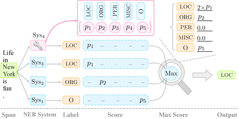
Figure 2: The framework of span prediction system (SpanNer) as system combiner. $p_{i}$ is calculated by function $\mathrm{score}(\cdot)$, as defined in Eq.4. $\mathrm{score}(\cdot)$ takes a span and predicted label as input and output a matching score. For example, $\mathrm{score}(\texttt{New York},\texttt{LOC})=0.5$ suggests that span “New York” matches “LOC” with the score of 0.5.

The prediction labels of the other three base models are “LOC”, “ORG”, and “O”, respectively. Then, as a combiner, SpanNer calculates the score for each predicted label. We sum weights (scores) of the same label that are predicted by the base models and select the label that achieves the maximum score as the output of the combiner.

5 Experiment

5.1 Base Systems

To make a thorough evaluation of SpanNer as a system combiner, as illustrated in Tab. 9, we first implement 10 SeqLab based systems that cover rich combinations of popular neural components. To be fair for other system combination methods, we also include two SpanNers as base systems. To reduce the uncertainty, we run experiments with multiple trials and also perform the significant test with Wilcoxon Signed-Rank Test Wilcoxon et al. (1970) at $p<0.05$.

Regarding SeqLab-base systems, following Fu et al. (2020b), their designs are diverse in four components: (1) character/subword-sensitive representation: ELMo (Peters et al., 2018), Flair (Akbik et al., 2018, 2019), BERT  (Devlin et al., 2018) 2) word representation: GloVe (Pennington et al., 2014), fastText (Bojanowski et al., 2017); (3) sentence-level encoders: LSTM (Hochreiter and Schmidhuber, 1997), CNN (Kalchbrenner et al., 2014b; Chen et al., 2019); (4) decoders: CRF (Lample et al., 2016; Collobert et al., 2011). We keep the testing result from the model with the best performance on the development set, terminating training when the performance of the development set is not improved in 20 epochs.

5.2 Baselines

We extensively explore six system combination methods as competitors, which involves supervised and unsupervised fashions.

5.2.1 Voting-based Approaches

Voting, as an unsupervised method, has been commonly used in existing works:

Majority voting (VM): All the individual classifiers are combined into a final system based on the majority voting.

Weighted voting base on overall F1-score (VOF1): The taggers are combined according to the weights, which is the overall F1-score on the testing set.

Weighted voting base on class F1-score (VCF1): Also weighted voting, the weights are the categories’ F1-score.

Cm	Best	SpNER	Voting-based			Stacking-based			Best	SpNER	Voting-based			Stacking-based
			VM†	VOF1†	VCF1†	SVM†	RF†	XGB†			VM†	VOF1†	VCF1†	SVM†	RF†	XGB†
	CoNLL-2003 (EN)								OntoNotes5.0-BN (BN)
all	93.02	93.80	93.62	93.57	93.60	93.28	93.04	92.93	90.93	91.14	90.92	91.29	91.12	89.67	90.95	90.50
m[:10]	93.02	93.78	93.48	93.55	93.54	93.21	93.03	93.18	90.93	91.48	91.03	91.41	91.27	89.97	90.92	90.91
m[:9]	93.02	93.81	93.57	93.59	93.51	93.33	93.26	93.35	90.93	91.64	91.16	91.24	91.22	90.16	90.75	90.76
m[:8]	93.02	93.81	93.41	93.52	93.54	93.28	93.17	93.14	90.93	91.74	91.17	91.59	91.39	90.16	90.69	90.81
m[:7]	93.02	93.72	93.41	93.47	93.41	93.26	92.98	93.00	90.93	91.86	91.60	91.66	91.57	90.16	90.80	90.73
m[:6]	93.02	93.71	93.21	93.63	93.53	93.20	93.27	93.21	90.93	91.95	91.42	91.74	91.67	90.34	91.09	91.04
m[:5]	93.02	93.80	93.46	93.54	93.52	93.33	93.19	93.28	90.93	90.65	91.69	91.77	91.97	90.54	90.72	90.69
m[:4]	93.02	93.70	93.29	93.69	93.61	93.47	93.20	93.28	90.93	90.30	91.18	91.13	90.32	90.02	90.93	90.77
m[:3]	93.02	93.75	93.66	93.75	93.61	93.30	93.38	93.43	90.93	91.13	91.07	91.13	91.13	90.89	90.98	91.08
m[:2]	93.02	93.01	93.02	92.99	92.95	92.74	92.86	92.86	90.93	89.81	90.70	89.78	90.01	90.61	90.98	90.81
m[2:4]	92.41	93.66	92.41	92.46	92.78	92.32	92.37	92.51	90.53	90.23	88.54	90.53	89.10	89.38	90.26	90.18
m[4:6]	92.11	93.39	92.01	92.11	92.31	92.01	92.15	92.17	89.43	90.80	89.33	89.43	89.77	89.66	89.49	89.99
m[3:6]	92.28	93.04	92.97	92.92	92.95	92.18	92.52	92.46	89.66	90.98	90.82	90.96	90.90	89.48	90.59	90.56
m[1:]	92.46	93.68	93.59	93.54	93.55	93.07	92.83	93.00	90.70	91.21	90.81	90.94	90.91	89.50	90.90	90.56
m[2:]	92.41	93.58	93.43	93.40	93.34	93.06	92.96	92.89	90.53	90.97	90.54	90.86	90.74	89.29	90.72	90.53
m[3:]	92.28	93.58	93.35	93.41	93.35	93.09	92.81	92.81	89.66	90.71	90.25	90.38	90.31	89.05	90.26	90.10
m[4:]	92.11	93.50	92.86	93.21	93.10	92.88	92.79	92.68	89.43	90.70	89.46	89.89	89.84	89.10	89.20	89.05
m[5:]	92.01	93.54	92.67	92.84	92.78	92.81	92.85	92.65	89.33	90.39	89.46	89.42	89.58	88.61	89.32	88.93
m[6:]	91.99	93.32	91.85	92.51	92.34	92.16	92.58	92.51	89.21	89.94	88.51	89.27	89.08	88.56	88.75	88.57
m[7:]	91.57	92.66	90.92	91.55	91.29	91.93	92.20	92.02	89.03	89.42	88.33	88.33	88.62	88.00	87.87	87.86
m[8:]	90.88	91.29	87.39	90.65	90.32	90.98	90.90	90.83	86.84	88.52	86.50	87.61	87.19	86.35	87.14	87.10
m[9:]	89.71	91.21	85.97	87.31	86.27	89.68	89.50	89.56	86.18	88.36	85.87	86.27	86.20	85.34	86.20	86.01
m[10:]	83.03	85.65	78.49	83.03	81.83	83.06	83.17	83.17	83.87	86.52	81.05	83.87	83.39	82.25	83.94	83.86
Std.	–	1.76	3.50	2.48	2.78	2.19	2.15	2.16	–	1.28	2.44	1.95	2.01	1.97	1.84	1.85
Avg.	91.98	93.00	91.83	92.36	92.22	92.24	92.22	92.21	89.73	90.45	89.63	90.02	89.88	89.00	89.72	89.63

Table 4: System combination results on CoNLL-2003 (EN) and OntoNotes5.0-BN (BN) datasets. SpNER denotes SpanNer while all setting denotes that all the models are putting together. Avg. and Std. represents the Average and Standard Deviation, respectively. $\mathbf{m}[i:k]$ is a group of models whose performance descending ranking are located on $[i,k)$. Best denotes the best performance of the single model on a model group $\mathbf{m}[i:k]$. ${\dagger}$ shows that the combined result of the baseline is significantly worse than the SpanNer (with Wilcoxon Signed-Rank Test at $p<0.05$). The values in bold indicate the best-combined results.

5.2.2 Stacking-based Approaches

Stacking (a.k.a, Stacked Generalization) is a general method of using a high-level model to combine lower-level models to achieve greater predictive accuracy Ting and Witten (1997). To make a comprehensive evaluation, we investigated three popular methods that are supervised learning, thereby requiring additional training samples. Specifically, there are:

Support Vector Machines (SVM) Hearst et al. (1998) is a supervised machine learning algorithm, which can train quickly over large datasets. Therefore, the ensemble classifier is usually SVM.

Random Forest (RF) Breiman (2001) is a common ensemble classifier that randomly selects a subset of training samples and variables to make multiple decision trees.

Extreme Gradient Boosting (XGB) Chen and Guestrin (2016) is also an ensemble machine learning algorithm. It is based on the decision-tree and the gradient boosting decision Friedman et al. (2000).

Notably, compared to our model, these methods are computationally expensive since they require external training samples for system combiners, which is achieved by (i) collecting training data by performing five-fold cross-validation Wu et al. (2003); Florian et al. (2003) on the original training samples of each dataset (ii) training a system combiner based on collected samples.

5.3 Exp-III: Nuanced View

Setup

Most previous works on system combination only consider one combination case where all base systems are put together. In this setting, we aim to explore more fine-grained combination cases. Specifically, we first sort systems based on their performance in a descending order to get a list $\mathbf{m}$. We refer to $\mathbf{m}[i:k]$ as one combination case, dubbed combined interval, which represents systems whose ranks are between $i$ and $k$. In practice, we consider 23 combination cases showing in Tab. 4. To examine whether the SpanNner is significantly better than the other baseline methods, we conduct the significance test with Wilcoxon Signed-RankTest Wilcoxon et al. (1970) at $p<0.05$.

Results

Tab. 4 shows results of our SpanNer against six baseline combiner methods on CoNLL-2003 and OntoNotes5.0-BN under a nuanced view. We can observe that:

(1) Overall, our proposed SpanNer outperforms all other competitors significantly (p-value $<$ 0.05) on most of the combination cases include the one (“all”) that most previous works have explored.

(2) As more base systems are introduced in descending order, the combined performance will be improved gradually. The combination performance will decrease with the reduction of the best single system, which holds for all the combiners.

(3) The best performance is always achieved on the combination case with more models, instead of the one with a small number of top-scoring base models. This suggests that introducing more base models with diverse structures will provide richer complementary information.

5.4 Exp-IV: Aggregated View

Setup

To also explore the effectiveness of SpanNer on the other datasets, we calculate the average performance of each system combination method over 23 combination cases.

Results

Tab. 5 shows the results, and we can observe that: comparing with the three voting combiner, SpanNer achieves the best average combination performance with the lowest standard deviation, which holds for seven of nine testing datasets with statistical significance p$<$0.05. Specifically, the performance gap between SpanNer and other combiners is larger on datasets from web domain: WB and Twitter: W16, W17.

Data	SpanNer		VM		VOF1		VCF1
	Avg.	Std.	Avg.	Std.	Avg.	Std.	Avg.	Std.
NW	90.78†	1.1	90.30	1.4	90.42	1.4	90.44	1.3
BC	81.54†	1.7	80.04	3.6	80.51	3.1	80.65	3.0
MZ	89.17	1.3	88.43	3.2	88.96	2.0	89.57	2.2
WB	67.45†	2.5	64.57	5.3	65.33	5.0	66.14	4.6
TC	68.25	3.8	66.16	6.5	67.54	5.6	68.73	5.5
W16	41.60†	6.4	33.23	9.2	36.19	8.9	39.92	7.9
W17	45.97†	6.1	41.27	9.3	43.32	8.2	44.45	7.7
ES	87.26†	2.6	86.23	4.3	87.24	2.8	87.00	2.8
NL	89.92†	3.4	87.59	6.5	88.93	4.7	88.66	5.0

Table 5: The average system combination results on 23 combination cases of nine datasets. Avg. and Std. denotes Average and Standard Deviation, respectively. ${\dagger}$ denotes that the SpanNer is better than the best baseline combiner significantly (p $<$ 0.05). The values in bold represent the best combination results.

5.5 Exp-VI: Interpretable Analysis

Setup

The above experiments have shown the superior performance of SpanNer on system combination. To further investigate where the gains of the SpanNer come from, similar to §3.3, we perform fine-grained evaluation on CoNLL-2003 dataset using one combination case to interpret how SpanNer outperform other (i) base systems and (ii) other baseline combiners. The combination case contains base systems: $sq0$-$5$ together with $sp1$, $sp2$ (model’s detail can refer to Tab.9).

Results

As shown in Tab. 6, we can find:

(1) SpanNer v.s. Base systems: the improvements of all base systems largely come from entities with low label consistency (eCon: XS, S). Particularly, base systems with SeqLab benefit a lot from short entities while base systems with SpanNer gain mainly from long entities.

(2) SpanNer v.s. Other combiners: as a system combiner, the improvement of SpanNer against other baselines mainly comes from low label consistency (eCon: XS, S). By contrast, traditional combiners surpass SpanNer when dealing with long sentences (sLen: XL).

SpanNer v.s. Base systems
eCon	sLen	eLen	oDen
SpanNer v.s. Other combiners
eCon	sLen	eLen	oDen

Table 6: Performance heatmap driven diagnosis analysis over different entity attributes. Each entry value is the F1 difference between the proposed SpanNer combiner against the Base systems (e.g., seq2 in Tab.9 ) or other combiners (e.g., VM: majority voting in §5.2.1) respectively. The green area indicates SpanNer combiner perform better.

6 Related Work

NER as Different Tasks

Although NER is commonly formulated as a sequence labeling task Chiu and Nichols (2015); Huang et al. (2015); Ma and Hovy (2016); Lample et al. (2016); Akbik et al. (2018); Peters et al. (2018); Devlin et al. (2018); Xia et al. (2019); Akbik et al. (2019); Luo et al. (2020); Lin et al. (2020), recently other new forms of frameworks have been explored and have shown impressive results. For example, (Jiang et al., 2020; Ouchi et al., 2020; Yu et al., 2020) shift NER from token-level tagging to span-level prediction task while (Li et al., 2020; Mengge et al., 2020) conceptualize it as reading comprehension task. In this work we aim to interpret the complementarity between sequence labeling and span prediction.

System Combination

Traditionally, system combination was used to improve the performance of statistical MT systems (González-Rubio et al., 2011; Watanabe and Sumita, 2011; Duh et al., 2011; Mizumoto and Matsumoto, 2016). Some recent work (Zhou et al., 2017; Huang et al., 2020) also extended this method to neural MT where the meta-model and base systems are all neural models. There is a handful of works about system combination for NER. Wu et al. (2003); Florian et al. (2003) investigated stacking and voting methods for combining strong classifiers. Ekbal and Saha (2011); Zhang et al. (2014) proposes a weighted voting approach based on differential evolution. These works commonly require training samples and rely heavily on feature engineering.

7 Implications and Future Directions

Co-evolution of NLP Systems and their combiners

Systems for NLP tasks (e.g., NER model) and their combiners (e.g., ensemble learning for NER) are developing in two parallel directions. This paper builds the connection between them and proposes a model that can be utilized as both a base NER system and a system combiner. Our work opens up a direction toward making the algorithms of NLP models and system combination co-evolved. The unified idea can be applied to other NLP tasks, and some traditional methods like re-ranking in syntactic parsing can be re-visited. For example, we can formulate constituency parsing Jiang et al. (2020) as well as its re-ranking Collins and Koo (2005); Huang (2008) as a span prediction Stern et al. (2017) problem, which is be unified and parameterized with the same form.

CombinaBoard

It has become a trend to use a Leaderboard (e.g., paperwithcode) to track current progress in a particular field, especially with the rapid emergence of a plethora of models. Leaderboard makes us pay more attention to and even obsess over the state-of-the-art systems Ethayarajh and Jurafsky (2020). We argue that Leaderboard with an effective system combination (dubbed CombinaBoard) feature would allow researchers to quickly find the complementarities among different systems. As a result, the value of a worse-ranked model still could be observed through its combined results. In this paper, we make the first step towards this by releasing a preliminary CombinaBoard for the NER task http://spanner.sh. Our model also has been deployed into the ExplainaBoard Liu et al. (2021) platform, which allows users to flexibly perform system combination of top-scoring systems in an interactive way: http://explainaboard.nlpedia.ai/leaderboard/task-ner/

Appendix A Attribute Interval

The detailed attribute interval for attributes: eCon, sLen, eLen, and oDen.

Bucket	eCon	sLen	eLen	oDen
XS	[0.0]	[1, 7]	[1]	[0]
S	[0, 0.5]	[7, 16]	[2]	[0, 0.067]
L	[0.5, 0.999]	[16, 31]	[3]	[0.067, 0.203]
XL	[1.0]	[31, 124]	[3, 6.0]	[0.203, 1.0]

Table 7: The attribute interval of bucket XS, S, L, and XL for attributes eCon, sLen, eLen, and oDen.

Models	Char/Sub.					Word			Sent.
	none	cnn	elmo	flair	bert	none	rand	glove	lstm	cnn
CflairWglove_lstmCrf (sq0)				$\surd$				$\surd$	$\surd$
CflairWnone_lstmCrf (sq1)				$\surd$		$\surd$			$\surd$
CbertWglove_lstmCrf (sq2)					$\surd$			$\surd$	$\surd$
CbertWnon_lstmCrf (sq3)					$\surd$	$\surd$			$\surd$
CelmoWglove_lstmCrf (sq4)			$\surd$					$\surd$	$\surd$
CelmoWnone_lstmCrf (sq5)			$\surd$			$\surd$			$\surd$
CcnnWglove_lstmCrf (sq6)		$\surd$						$\surd$	$\surd$
CcnnWglove_cnnCrf (sq7)		$\surd$						$\surd$		$\surd$
CcnnWrand_lstmCrf (sp8)		$\surd$					$\surd$		$\surd$
CnoneWrand_lstmCrf (sp9)	$\surd$						$\surd$		$\surd$

Table 8: The illustration of SeqLab’s model name and its structures. “Sub”, “sent.” and “Dec.” denotes the subword embedding, sentence encoder, and decoder, respectively. All the ten sequence labeling models use the CRF as the decoder. $\surd$ indicates the embedding/structure is utilized in the current SeqLab system.

Appendix B Model Name illustration of SeqLab

Tab. 8 illustrates the full model name and the detailed structure of the SeqLab models. All the SeqLab models use the CRF as the decoder. For example, the full model name of “sq0” is “CflairWglove_lstmCrf”, representing a sequence labeling model that uses the Flair as character-level embedding, GloVe as word-level embedding, LSTM as the sentence-level encoder, and CRF as the decoder. For “sq3”, its full model name is “CbertWnon_lstmCrf”, representing a sequence labeling model that uses the BERT as character-level embedding, LSTM as the sentence-level encoder, and CRF as the decoder.

References

- Akbik et al. (2019) Alan Akbik, Tanja Bergmann, and Roland Vollgraf. 2019. Pooled contextualized embeddings for named entity recognition. In Proceedings of the 2019 Conference of the North American Chapter of the Association for Computational Linguistics: Human Language Technologies, Volume 1 (Long and Short Papers), pages 724–728.
- Akbik et al. (2018) Alan Akbik, Duncan Blythe, and Roland Vollgraf. 2018. Contextual string embeddings for sequence labeling. In Proceedings of the 27th International Conference on Computational Linguistics, pages 1638–1649.
- Bojanowski et al. (2017) Piotr Bojanowski, Edouard Grave, Armand Joulin, and Tomas Mikolov. 2017. Enriching word vectors with subword information. Transactions of the Association for Computational Linguistics, 5:135–146.
- Breiman (2001) Leo Breiman. 2001. Random forests. Machine learning, 45(1):5–32.
- Chen et al. (2019) Hui Chen, Zijia Lin, Guiguang Ding, Jianguang Lou, Yusen Zhang, and Borje Karlsson. 2019. Grn: Gated relation network to enhance convolutional neural network for named entity recognition. Thirty-Third AAAI Conference on Artificial Intelligence, 33(01):6236–6243.
- Chen and Guestrin (2016) Tianqi Chen and Carlos Guestrin. 2016. Xgboost: A scalable tree boosting system. In Proceedings of the 22nd acm sigkdd international conference on knowledge discovery and data mining, pages 785–794.
- Chiu and Nichols (2015) Jason PC Chiu and Eric Nichols. 2015. Named entity recognition with bidirectional lstm-cnns. arXiv preprint arXiv:1511.08308.
- Collins and Koo (2005) Michael Collins and Terry Koo. 2005. Discriminative reranking for natural language parsing. Computational Linguistics, 31(1):25–70.
- Collobert et al. (2011) Ronan Collobert, Jason Weston, Léon Bottou, Michael Karlen, Koray Kavukcuoglu, and Pavel Kuksa. 2011. Natural language processing (almost) from scratch. Journal of Machine Learning Research, 12(Aug):2493–2537.
- Derczynski et al. (2017) Leon Derczynski, Eric Nichols, Marieke van Erp, and Nut Limsopatham. 2017. Results of the wnut2017 shared task on novel and emerging entity recognition. In Proceedings of the 3rd Workshop on Noisy User-generated Text, pages 140–147.
- Devlin et al. (2018) Jacob Devlin, Ming-Wei Chang, Kenton Lee, and Kristina Toutanova. 2018. Bert: Pre-training of deep bidirectional transformers for language understanding. arXiv preprint arXiv:1810.04805.
- Devlin et al. (2019) Jacob Devlin, Ming-Wei Chang, Kenton Lee, and Kristina Toutanova. 2019. Bert: Pre-training of deep bidirectional transformers for language understanding. In NAACL-HLT (1).
- Duh et al. (2011) Kevin Duh, Katsuhito Sudoh, Xianchao Wu, Hajime Tsukada, and Masaaki Nagata. 2011. Generalized minimum bayes risk system combination. In Proceedings of 5th International Joint Conference on Natural Language Processing, pages 1356–1360.
- Durrett and Klein (2014) Greg Durrett and Dan Klein. 2014. A joint model for entity analysis: Coreference, typing, and linking. Transactions of the association for computational linguistics, 2:477–490.
- Ekbal and Saha (2011) Asif Ekbal and Sriparna Saha. 2011. Weighted vote-based classifier ensemble for named entity recognition: A genetic algorithm-based approach. ACM Transactions on Asian Language Information Processing (TALIP), 10(2):1–37.
- Ethayarajh and Jurafsky (2020) Kawin Ethayarajh and Dan Jurafsky. 2020. Utility is in the eye of the user: A critique of NLP leaderboards. In Proceedings of the 2020 Conference on Empirical Methods in Natural Language Processing (EMNLP), pages 4846–4853, Online. Association for Computational Linguistics.
- Florian et al. (2003) Radu Florian, Abe Ittycheriah, Hongyan Jing, and Tong Zhang. 2003. Named entity recognition through classifier combination. In Proceedings of the seventh conference on Natural language learning at HLT-NAACL 2003, pages 168–171.
- Friedman et al. (2000) Jerome Friedman, Trevor Hastie, Robert Tibshirani, et al. 2000. Additive logistic regression: a statistical view of boosting (with discussion and a rejoinder by the authors). Annals of statistics, 28(2):337–407.
- Fu et al. (2021) Jinlan Fu, Liangjing Feng, Qi Zhang, Xuanjing Huang, and Pengfei Liu. 2021. Larger-context tagging: When and why does it work? arXiv preprint arXiv:2104.04434.
- Fu et al. (2020a) Jinlan Fu, Pengfei Liu, and Graham Neubig. 2020a. Interpretable multi-dataset evaluation for named entity recognition. In Proceedings of the 2020 Conference on Empirical Methods in Natural Language Processing (EMNLP), pages 6058–6069, Online. Association for Computational Linguistics.
- Fu et al. (2020b) Jinlan Fu, Pengfei Liu, and Qi Zhang. 2020b. Rethinking generalization of neural models: A named entity recognition case study. In Proceedings of the AAAI Conference on Artificial Intelligence, volume 34, pages 7732–7739.
- Fu et al. (2020c) Jinlan Fu, Pengfei Liu, Qi Zhang, and Xuanjing Huang. 2020c. RethinkCWS: Is Chinese word segmentation a solved task? In Proceedings of the 2020 Conference on Empirical Methods in Natural Language Processing (EMNLP), pages 5676–5686, Online. Association for Computational Linguistics.
- Ghaddar and Langlais (2018) Abbas Ghaddar and Philippe Langlais. 2018. Robust lexical features for improved neural network named-entity recognition. arXiv preprint arXiv:1806.03489.
- González-Rubio et al. (2011) Jesús González-Rubio, Alfons Juan, and Francisco Casacuberta. 2011. Minimum Bayes-risk system combination. In Proceedings of the 49th Annual Meeting of the Association for Computational Linguistics: Human Language Technologies, pages 1268–1277, Portland, Oregon, USA. Association for Computational Linguistics.
- Hearst et al. (1998) Marti A. Hearst, Susan T Dumais, Edgar Osuna, John Platt, and Bernhard Scholkopf. 1998. Support vector machines. IEEE Intelligent Systems and their applications, 13(4):18–28.
- Hochreiter and Schmidhuber (1997) Sepp Hochreiter and Jürgen Schmidhuber. 1997. Long short-term memory. Neural computation, 9(8):1735–1780.
- Huang (2008) Liang Huang. 2008. Forest reranking: Discriminative parsing with non-local features. In Proceedings of ACL-08: HLT, pages 586–594, Columbus, Ohio. Association for Computational Linguistics.
- Huang et al. (2020) Xuancheng Huang, Jiacheng Zhang, Zhixing Tan, Derek F. Wong, Huanbo Luan, Jingfang Xu, Maosong Sun, and Yang Liu. 2020. Modeling voting for system combination in machine translation. In Proceedings of the Twenty-Ninth International Joint Conference on Artificial Intelligence, IJCAI 2020, pages 3694–3701. ijcai.org.
- Huang et al. (2015) Zhiheng Huang, Wei Xu, and Kai Yu. 2015. Bidirectional lstm-crf models for sequence tagging. arXiv preprint arXiv:1508.01991.
- Jiang et al. (2020) Zhengbao Jiang, Wei Xu, Jun Araki, and Graham Neubig. 2020. Generalizing natural language analysis through span-relation representations. In Proceedings of the 58th Annual Meeting of the Association for Computational Linguistics, pages 2120–2133, Online. Association for Computational Linguistics.
- Kalchbrenner et al. (2014a) Nal Kalchbrenner, Edward Grefenstette, and Phil Blunsom. 2014a. A convolutional neural network for modelling sentences. In Proceedings of the 52nd Annual Meeting of the Association for Computational Linguistics (Volume 1: Long Papers), pages 655–665, Baltimore, Maryland. Association for Computational Linguistics.
- Kalchbrenner et al. (2014b) Nal Kalchbrenner, Edward Grefenstette, and Phil Blunsom. 2014b. A convolutional neural network for modelling sentences. In Proceedings of ACL.
- Kim (2014) Yoon Kim. 2014. Convolutional neural networks for sentence classification. In Proceedings of the 2014 Conference on Empirical Methods in Natural Language Processing (EMNLP), pages 1746–1751, Doha, Qatar. Association for Computational Linguistics.
- Lample et al. (2016) Guillaume Lample, Miguel Ballesteros, Sandeep Subramanian, Kazuya Kawakami, and Chris Dyer. 2016. Neural architectures for named entity recognition. In Proceedings of NAACL-HLT, pages 260–270.
- Lewis et al. (2020) Mike Lewis, Yinhan Liu, Naman Goyal, Marjan Ghazvininejad, Abdelrahman Mohamed, Omer Levy, Veselin Stoyanov, and Luke Zettlemoyer. 2020. BART: Denoising sequence-to-sequence pre-training for natural language generation, translation, and comprehension. In Proceedings of the 58th Annual Meeting of the Association for Computational Linguistics, pages 7871–7880, Online. Association for Computational Linguistics.
- Li et al. (2020) Xiaoya Li, Jingrong Feng, Yuxian Meng, Qinghong Han, Fei Wu, and Jiwei Li. 2020. A unified MRC framework for named entity recognition. In Proceedings of the 58th Annual Meeting of the Association for Computational Linguistics, pages 5849–5859, Online. Association for Computational Linguistics.
- Lin et al. (2020) Bill Yuchen Lin, Dong-Ho Lee, Ming Shen, Ryan Moreno, Xiao Huang, Prashant Shiralkar, and Xiang Ren. 2020. Triggerner: Learning with entity triggers as explanations for named entity recognition. In Proceedings of the 58th Annual Meeting of the Association for Computational Linguistics, pages 8503–8511.
- Liu et al. (2021) Pengfei Liu, Jinlan Fu, Yang Xiao, Weizhe Yuan, Shuaicheng Chang, Junqi Dai, Yixin Liu, Zihuiwen Ye, and Graham Neubig. 2021. Explainaboard: An explainable leaderboard for nlp. arXiv preprint arXiv:2104.06387.
- Liu and Lapata (2019) Yang Liu and Mirella Lapata. 2019. Text summarization with pretrained encoders. In Proceedings of the 2019 Conference on Empirical Methods in Natural Language Processing and the 9th International Joint Conference on Natural Language Processing (EMNLP-IJCNLP), pages 3730–3740, Hong Kong, China. Association for Computational Linguistics.
- Luo et al. (2020) Ying Luo, Fengshun Xiao, and Hai Zhao. 2020. Hierarchical contextualized representation for named entity recognition. In Proceedings of the AAAI Conference on Artificial Intelligence, volume 34, pages 8441–8448.
- Ma and Hovy (2016) Xuezhe Ma and Eduard Hovy. 2016. End-to-end sequence labeling via bi-directional lstm-cnns-crf. In Proceedings of the 54th Annual Meeting of ACL, volume 1, pages 1064–1074.
- Mengge et al. (2020) Xue Mengge, Bowen Yu, Zhenyu Zhang, Tingwen Liu, Yue Zhang, and Bin Wang. 2020. Coarse-to-fine pre-training for named entity recognition. In Proceedings of the 2020 Conference on Empirical Methods in Natural Language Processing (EMNLP), pages 6345–6354.
- Mizumoto and Matsumoto (2016) Tomoya Mizumoto and Yuji Matsumoto. 2016. Discriminative reranking for grammatical error correction with statistical machine translation. In Proceedings of the 2016 Conference of the North American Chapter of the Association for Computational Linguistics: Human Language Technologies, pages 1133–1138, San Diego, California. Association for Computational Linguistics.
- Ouchi et al. (2020) Hiroki Ouchi, Jun Suzuki, Sosuke Kobayashi, Sho Yokoi, Tatsuki Kuribayashi, Ryuto Konno, and Kentaro Inui. 2020. Instance-based learning of span representations: A case study through named entity recognition. arXiv preprint arXiv:2004.14514.
- Pennington et al. (2014) Jeffrey Pennington, Richard Socher, and Christopher Manning. 2014. Glove: Global vectors for word representation. In Proceedings of the 2014 conference on empirical methods in natural language processing (EMNLP), pages 1532–1543.
- Peters et al. (2018) Matthew Peters, Mark Neumann, Mohit Iyyer, Matt Gardner, Christopher Clark, Kenton Lee, and Luke Zettlemoyer. 2018. Deep contextualized word representations. In Proceedings of the 2018 Conference of NAACL, volume 1, pages 2227–2237.
- Saha and Ekbal (2013) Sriparna Saha and Asif Ekbal. 2013. Combining multiple classifiers using vote based classifier ensemble technique for named entity recognition. Data & Knowledge Engineering, 85:15–39.
- Sang and De Meulder (2003) Erik F Sang and Fien De Meulder. 2003. Introduction to the conll-2003 shared task: Language-independent named entity recognition. arXiv preprint cs/0306050.
- Sang (2002) Erik F. Tjong Kim Sang. 2002. Introduction to the conll-2002 shared task: Language-independent named entity recognition. In Proceedings of the 6th Conference on Natural Language Learning, CoNLL 2002, Held in cooperation with COLING 2002, Taipei, Taiwan, 2002. ACL.
- Speck and Ngomo (2014) René Speck and Axel-Cyrille Ngonga Ngomo. 2014. Ensemble learning for named entity recognition. In International semantic web conference, pages 519–534. Springer.
- Stern et al. (2017) Mitchell Stern, Jacob Andreas, and Dan Klein. 2017. A minimal span-based neural constituency parser. arXiv preprint arXiv:1705.03919.
- Strauss et al. (2016) Benjamin Strauss, Bethany Toma, Alan Ritter, Marie-Catherine De Marneffe, and Wei Xu. 2016. Results of the wnut16 named entity recognition shared task. In Proceedings of the 2nd Workshop on Noisy User-generated Text (WNUT), pages 138–144.
- Ting and Witten (1997) Kai Ming Ting and Ian H. Witten. 1997. Stacked generalizations: When does it work? In Proceedings of the Fifteenth International Joint Conference on Artificial Intelligence, IJCAI 97, Nagoya, Japan, August 23-29, 1997, 2 Volumes, pages 866–873. Morgan Kaufmann.
- Watanabe and Sumita (2011) Taro Watanabe and Eiichiro Sumita. 2011. Machine translation system combination by confusion forest. In Proceedings of the 49th Annual Meeting of the Association for Computational Linguistics: Human Language Technologies, pages 1249–1257, Portland, Oregon, USA. Association for Computational Linguistics.
- Weischedel et al. (2013) Ralph Weischedel, Martha Palmer, Mitchell Marcus, Eduard Hovy, Sameer Pradhan, Lance Ramshaw, Nianwen Xue, Ann Taylor, Jeff Kaufman, Michelle Franchini, et al. 2013. Ontonotes release 5.0 ldc2013t19. Linguistic Data Consortium, Philadelphia, PA.
- Wilcoxon et al. (1970) Frank Wilcoxon, SK Katti, and Roberta A Wilcox. 1970. Critical values and probability levels for the wilcoxon rank sum test and the wilcoxon signed rank test. Selected tables in mathematical statistics, 1:171–259.
- Wu et al. (2003) Dekai Wu, Grace Ngai, and Marine Carpuat. 2003. A stacked, voted, stacked model for named entity recognition. In Proceedings of the seventh conference on Natural language learning at HLT-NAACL 2003, pages 200–203.
- Xia et al. (2019) Congying Xia, Chenwei Zhang, Tao Yang, Yaliang Li, Nan Du, Xian Wu, Wei Fan, Fenglong Ma, and S Yu Philip. 2019. Multi-grained named entity recognition. In Proceedings of the 57th Annual Meeting of the Association for Computational Linguistics, pages 1430–1440.
- Yamada et al. (2020) Ikuya Yamada, Akari Asai, Hiroyuki Shindo, Hideaki Takeda, and Yuji Matsumoto. 2020. LUKE: Deep contextualized entity representations with entity-aware self-attention. In Proceedings of the 2020 Conference on Empirical Methods in Natural Language Processing (EMNLP), pages 6442–6454, Online. Association for Computational Linguistics.
- Yu et al. (2020) Juntao Yu, Bernd Bohnet, and Massimo Poesio. 2020. Named entity recognition as dependency parsing. In Proceedings of the 58th Annual Meeting of the Association for Computational Linguistics, pages 6470–6476, Online. Association for Computational Linguistics.
- Zhang et al. (2014) Yong Zhang, Hongrui Zhang, Jing Cai, and Binbin Yang. 2014. A weighted voting classifier based on differential evolution. In Abstract and Applied Analysis, volume 2014. Hindawi.
- Zhou et al. (2017) Long Zhou, Wenpeng Hu, Jiajun Zhang, and Chengqing Zong. 2017. Neural system combination for machine translation. In Proceedings of the 55th Annual Meeting of the Association for Computational Linguistics (Volume 2: Short Papers), pages 378–384, Vancouver, Canada. Association for Computational Linguistics.