CoRank: A clustering cum graph ranking approach for extractive summarization

Abstract.

On-line information has increased tremendously in today’s age of Internet. As a result, the need has arose to extract relevant content from the plethora of available information. Researchers are widely using automatic text summarization techniques for extracting useful and relevant information from voluminous available information, it also enables users to obtain valuable knowledge in a limited period of time with minimal effort. The summary obtained from the automatic text summarization often faces the issues of diversity and information coverage. Promising results are obtained for automatic text summarization by the introduction of new techniques based on graph ranking of sentences, clustering, and optimization. This research work proposes CoRank, a two-stage sentence selection model involving clustering and then ranking of sentences. The initial stage involves clustering of sentences using a novel clustering algorithm, and later selection of salient sentences using CoRank algorithm.Te approach aims to cover two objectives: maximum coverage and diversity, which is achieved by the extraction of main topics and sub-topics from the original text. The performance of the CoRank is validated on DUC2001 and DUC 2002 data sets.

1. Introduction

Recently, multi-document summarization and document clustering have gained a lot of attention for analyzing textual information. The aim of document clustering is to divide a set of documents into distinct classes called clusters, where similar documents are occurring in same cluster and dissimilar documents (Duda et al., 2001) occurring in different clusters. Another efficient technique for extracting relevant content from huge volumnious data is multi-document summarization, that aims to create reduced summary while retaining the gist of the documents (Mani, 2001; Ricardo and Berthier, 1999). Both these techniques find a range of applications in information retrieval and management, apart from retrieving relevant content from documents. Results of web search (Zamir and Etzioni, 1998) can be organized and presented in an efficient way using document clustering. Apart from it, multi-document summarization finds its use in creation of snippet on the Web, that can be further used for future purposes (Turpin et al., 2007).

Usually researchers while performing document clustering consider the set of documents as document term matrix where documents are represented by rows and terms are represented by columns. Several conventional clustering algorithms exist for grouping the similar documents. But these algorithms were unable to correctly interpret the document cluster. In recent years, some works (Dhillon et al., 2001) have focused on capturing the dual knowledge between documents and terms and performing clustering at the same time. But this framework has limitation, since every document cluster is represented by a set of representative words, and these words cannot give a true interpretation of clusters as they lack contextual and semantic information. Another way could be selection of salient sentences from the cluster.

Multi-document summarization(MDS) aims at producing a condensed version of the document while retaining the girth of the document. Based on the output type, MDS can be categorized into abstractive or extractive. In extractive summarization, representative sentences are selected as summary from the original source document. This approach uses some pre-defined methodolgy to compute sentence scores and based on that salient sentences are seelcted. Whereas in abstractive summarization, summary is composed of salient sentences that represent the gist of the document but are not part of original document. Some techniques such as reformulation, sentence compression, and information fusion is involved in abstractive summarization. The summary obtained from abstractive summarization are compact since it uses deep learning techniques. This research work concentrates on extractive summarization since it is more practical and feasible. In MDS, the set of documents are represented as sentence-term matrix where rows and columns are represented as sentences and terms. Numerous clustering approaches (Jing and Mckeown, 2000; Knight and Marcu, 2002) have been proposed for extractive summarization where the first step is cluster generation and then identification of salient sentences from these clusters. The limitation of such approach is that they consider sentences as independent units and contextual dependency among sentences are ignored. However, the mutual influence of sentences occurring within same cluster should be considered for correct interpretation of cluster.

The focus of the proposed methodology in the research paper is to convert a document into an appropriate graph structure, cluster it into overlapping communities, and extract out most important sentences of the document. The novelty of the proposed research work is highlighted below:

1.1. Contributions

• The given textual document is converted into a graph. A novel algorithm is developed to detect overlapping communities in a weighted network with feasible computational requirements.

• A node can lie in several of the overlapping communities. This invalidates the assumption of the influential nodes algorithm on unweighted, distinct communities. We propose an inexpensive algorithm on top of the community detection to list out important nodes of the underlying graph.

• Larger subtopics in a document carry more importance than the smaller subtopics. The proposed CoRank method picks sentences depending on the weightage of subtopic.

• We conduct experiments on the standard DUC-2001 and DUC-2002 data-set to validate the performance of proposed CoRank method.

The further sections are divided as follows. Section 2 introduces overview of the work done in this area and connected relevant fields followed by a brief introduction of the problem statement given in Section 3. Section 4 discusses a step-by-step procedure for the proposed methodology. Section 5 discusses about the explanation of the proposed methodolgy using a toy network example. Section 6 describes in detail the analysis of the experiments followed by conclusion in Section 7.

2. Related Work

Extractive text summarization has been in active developments in recent years, numerous methods have been proposed to solve the problem. The key idea lies in developing an efficient scoring method for the sentences in the document. Many methods apply topic-wise clustering on the document and identifying key individual sentences with respect to the topics. Some other approaches revolve around using evolutionary algorithms (Mendoza et al., 2014b) or machine learning techniques (Ozsoy et al., 2011) (Jang and Kang, 2021).

2.1. Graph Based Approaches

The method proposed in (Cai and Li, 2011) simultaneously clusters the sentences and scores them for a ranking. The focus of work in (Alguliyev et al., 2017) is to cluster the sentences and perform their selection as a solution to an optimization problem. (Cai et al., 2014b) targets both diversity and coverage of the summary using an integrated clustering based technique. The idea in (Cai et al., 2014a) uses co-clustering method on words and sentences individually to perform a topic based summarization. The framework introduced allows words to have an explicit decision in sentence selection to squeeze out better performance. (Mei and Chen, 2012) proposes a fuzzy c-medoid based clustering approach to produce cluster of sentences similar to a subtopic of the topic. A tool named Compendium is proposed in (LLORET and Sanz, 2013), which combines textual entailment, statistical and cognition based techniques to remove redundant information and find relevant content in summary. The work in (Luo et al., 2013) focuses on probabilistic modelling topic relevance and coverage in summarization. In (Yang and Wang, 2008), the authors use fractal theory to infer the interplay of sentences and perform the summarization.

The work in (Ferreira et al., 2014) uses a graph based approach to cluster the sentences. Document is modelled as a graph and then the different methods are used to rank the sentences (modelled as nodes). (Li and Li, 2014) propose a semi-supervised clustering method on the graphs combined with topic modelling. In (Balaji et al., 2014), they use the ideas of graph matching to improve upon the results. (Wan et al., 007a) proposes Collabsum, which exploits information from multiple documents by clustering them and extracting the mutual influence to summarise a single document. This methodology incorporates both the intra-document and inter-document relationships. (Alguliev et al., 2012) models the summarization as a modified p-median problem. The work in (Hingu et al., 2015), uses external knowledge from Wikipedia to enhance performance on the existing graph based methods. In (Erkan and Radev, 2004), a novel LexRank method is introduced, it determines the salience using eigenvector centrality in graphical representation. The work in (Wan, 2010) models the documents as graph and exploits mutual information between documents to generate summary.

A separate line of work has evolved in community detection and influential node identification. (Yang et al., 2018) introduces TOPSIS to identify influential nodes by considering it as a multi-attribute decision-making problem. (Ding et al., 2016) proposes NDOCD where links are iteratively removed to reduce the graph into clusters. In (Zhang et al., 2020), the method proposed network embedding is used to decompose the network into communities and then nodes are chosen to maximize influence. (Ahmad et al., 2020) propose MHWSMCB, where various degrees are considered to choose influential nodes in a network as a influence maximization problem. The authors in (Gupta and Kumar, 2020) introduce an algorithm for overlapping community detection based on granular information of links and concepts of rough set theory.

2.2. Other Approaches

In (Mendoza et al., 2014b), a mematic algorithm MA-SingleDocSum is introduced, the method uses evolutionary algorithm to solve the extractive summarization as a binary optimization problem. (Yan and Guo, 2020) propose a hierarchical selective encoding network for both sentence-level and document-level representations and data containing important information is extracted. The method introduced in (Batista et al., 2016) improves upon the cohesiveness of the summaries generated by extractive summarization systems. It is based on a post-processing step that binds dangling co-reference to the most important entity in a given co-reference chain. In (Bonzanini et al., 2013) selectively removes unimportant sentences until a desired compression score is achieved. The work by (Sonawane et al., 2019) model the document as semi-graph to extract both linear and non-linear relationships between the features. In (Parveen et al., 2015), a weighted graphical representation of the document is formed and coherence, non-redundance and importance are optimized using ILP (Inductive logic programming). (Ozsoy et al., 2011) uses algorithms based on Latent Semantic Analysis to summarize Turkish and English text. (Jang and Kang, 2021) proposes a deep-learning method to perform unsupervised summarization. The researchers in (Nishino et al., 2013) use Langragian relaxation to solve summarization as combinatorial problem.

Several unsupervised algorithms have also been introduced to cluster the sentences and rank them. The methods use k-means (Shetty and Kallimani, 2017) or fuzzy c-means (Anam et al., 2018) due to their good generalization performance in other tasks also. Fuzzy c-means is not robust to noises and is sensitive to outliers in euclidean distance.

In (Begum et al., 2009), the method uses support vector machine (SVM) to train a summarizer using features like sentence position, sentence centrality, sentence similarity and several more. (Zopf et al., 2018) uses sentence regression to score and greedily selects them to form the summary. In (Chali et al., 2009), the authors train an ensemble of SVMs over gram overlap, LCS, WLCS, skip-bigram, gloss overlap,BE overlap, length of sentence, position of the sentence, NE, cue word match, title match to approach the problem.

3. Problem Statement

Given a document $D$ consisting set of sentences $D=\{s_{1},s_{2},s_{3},\dots s_{n}\}$, where $n$ denotes the number of sentences in the document and $s_{j}$ is the j-th sentence, $1\leq j\leq n$. The aim of of extractive summarization is to find a subset $D_{s}\subset D$ which contains different important topics mentioned in the complete document. It is expected to have $|D_{s}|\ll|D|$ where $|.|$ represent the number of sentences in the set.

A document consists of vast information covering various subtopics and a common main theme connecting them. Coverage means that the summary extracted by algorithm should cover most of the subtopics. Poor coverage of subtopics is indicated by absence of some relevant sentences. While extracting the sentences, deciding the importance based on relevance alone can be misleading and ignoring lesser covered but important subtopics. Therefore, focus of the algorithm on both relevance and coverage is necessary.

4. Methodology

4.1. Graph Construction

The document is split into sentences. Let the graph formed be $G=(V,E)$ where elements in set $V$ are the sentences and $E$ represent the set of edges between a pair of sentences. The presence of an edge between a pair of sentences is decided by a weighted sum of their statistical and semantic similarities. A hyperparameter, $\delta_{e}$ is chosen and if a pair has similarity lesser than $\delta_{e}$, no edge exists between them. Clearly, a high value of $\delta_{e}$ encourages lesser number of edges and a lower value will include all the $\binom{V}{2}$ edges in the graph. An appropriate threshold will retain relations between important sentences and discard edges between insignificant sentences. This workflow is represented in the figure 1

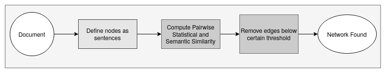
Figure 1. Flow diagram showing construction of graph-network from a given document.

4.2. Community Detection

The graph $G=(V,E)$ formed thus is a weighted graph, let $w_{i,j}$ represent weight of edge $e_{i,j}$ between node $v_{i}$ and node $v_{j}$. Additionally, it satisfies the condition: $w_{i,j}\geq\delta_{e}$ The figure 2 shows the flow diagram for this section of algorithm. The algorithm introduces terminoligies mentioned below:

1. FOAN: First Order Approximate Neighbors - First Order Approximate Neighbors of a link $e_{i,j}$ are defined by :

   (1) $$F(e_{i,j})=\{e_{i,k}:k\in N_{i}\}\cup\{e_{k,j}:k\in N_{j}\}$$

   where $N_{i}$ and $N_{j}$ represent the nodes connected to $v_{i}$ and $v_{j}$.

2. SOAN: Second Order Approximate Neighbors - Second Order Approximate Neighbors of a link $e_{i,j}$ are defined by :

   (2) $$S(e_{i,j})=\bigcup\{F(e_{m,n}):(m,n)\in F(e_{i,j})\}$$

3. JS: Jaccard Similarity - Jaccard Similarity between two vectors x and y is given by:

   (3) $$J_{\mathcal{W}}(\textbf{x},\textbf{y})=\frac{\sum_{i}min(x_{i},y_{i})}{\sum_{i}max(x_{i},y_{i})}$$

4. CSOAN: Constrained Second Order Approximate Neighbors - Constrained Second Order Approximate Neighbors of a link $e_{i,j}$ are defined by :

   (4) $$C(e_{i,j})=\{e_{a,b}:e_{a,b}\in S(e_{i,j})|J_{\mathcal{W}}(\overline{e}_{i,j},\overline{e}_{a,b})\geq\delta_{csoan}\}$$

5. LNS: Link Node Set - Link Node Set of a link $e_{i,j}$ is defined by :

   (5) $$L(e_{i,j})=\{v_{m},v_{n}:e_{m,n}\in C(e_{i,j})\}$$

   So, $L(e_{i,j})\subset V$ whereas $C(e_{i,j})\subset E$, $S(e_{i,j})\subset E$, and $F(e_{i,j})\subset E$.

6. Conductance - Conductance of a graph $G=(V,E)$ is given by :

   (6) $$\phi(G)=\min_{S\in V;0\leq a(S)\leq a(V)/2}\frac{\sum_{i\in S;j\in\overline{S}}a_{i,j}}{a(S)}$$

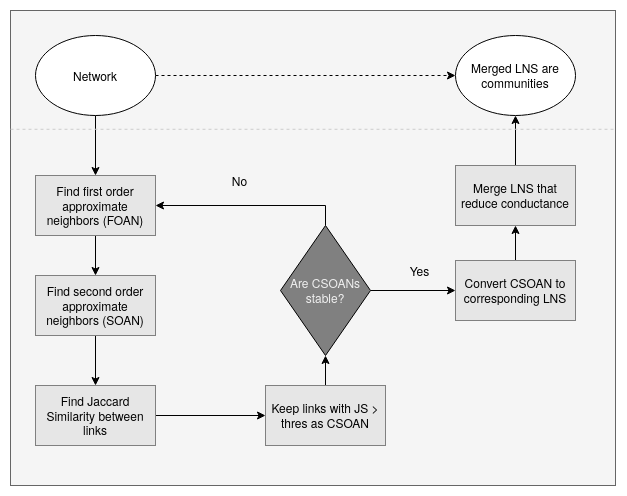
Figure 2. Flow diagram showing detection of communities by the algorithm.

The algorithm processes the graph of document through several steps iteratively unless a stable set of edges is obtained. A set of first order approximate neighbors is formed for every edge in graph, using the equation 1. Next, a set of second order approximate neighbors is formed by the union of first order approximate neighbors of every edge in the first order approximate neighbors of the target edge (equation 2). The cardinality of this set determines the number of nodes which share a strong similarity with the nodes of given edge. The sum of the weights of the elements in $S(e_{i,j})$ is higher for an edge with greater importance in the graph. Every set $F(e_{i,j}$ can be represented as vector with orthogonal components corresponding to the weight of edge elements. So every edge $e_{i,j}$ has a $S(e_{i,j})$ which can be expressed as a vector $\overline{e}_{i,j}$, given by equation 7.

(7) $$\overline{e}_{i,j}=\sum_{t\in S(e_{i,j})}w_{t}\cdot\hat{t}$$

For every pair of edges in the graph $e_{i,j}$ and $e_{m,n}$, Jaccard Similarity is calculated between their corresponding vectors $\overline{e}_{i,j}$ and $\overline{e}_{m,n}$ using equation 3. A higher coefficients for an edge indicate greater similarity and higher importance than the other edges. The coefficients found are used to filter out edges with low similarity in $S(e_{i,j})$. A threshold $\delta_{cson}$ is used to calculate the constrained second order approximate neighbors $C(e_{i,j})$ using equation 4. The set $C(e_{i,j})$ is used as $F(e_{i,j})$ in the next iterative step (if need be). The loop stops processing an edge $e_{i,j}$ when the $C(e_{i,j})$ for a step is same as $C(e_{i,j})$ in previous iteration, and the set $C(e_{i,j})$ is deemed stable.

When stable sets of $C(e_{i,j})$ for every edge $e_{i,j}$ are found out, loop completely terminates. Every set $C(e_{i,j})$ is used to make the corresponding link node set $L(e_{i,j})$ using equation 5. Next, conductance of every $L(e_{i,j})$ is calculated using equation 6. A pair of $L(e_{i,j})$ and $L(e_{m,n})$ are merged if the resultant set $L(e_{i,j})\cup L(e_{m,n})$ has a conductance lower than the individual sets. $L(e_{i,j})$ are merged (union) until conductance can no longer be reduced. The resultant set of node sets correspond to the communities detected.

4.3. Finding Important Sentences

Finding most significant sentences in document network is equivalent to finding most influential nodes in a network. Let the communities detected by following algorithm in section 4.2 are $\mathcal{H}$. The subgraphs formed using $G=(V,E)$ and nodes in $H_{i}\in H$ are overlapping in nature, hence the influence of a node in graph $G$ is determined by the influence in $H_{i}$ and also by $H_{j}\in\mathcal{H},j\neq i$.

For every subgraph using nodes of $H_{i}\in\mathcal{H}$, weighted degree of each node is calculated. A larger weighted degree of a node signifies larger influence in the community. Additionally, a larger community is responsible for larger influence in the graph. So, the algorithm picks largest community and the node with largest weighted degree. This node is removed from the community and again the algorithm picks. The step mentioned is iteratively done until a desired number of nodes are extracted. The figure 3 shows the flow diagram for this section of algorithm. where $N_{i}$ and $N_{j}$ represent the nodes connected to $v_{i}$ and $v_{j}$.

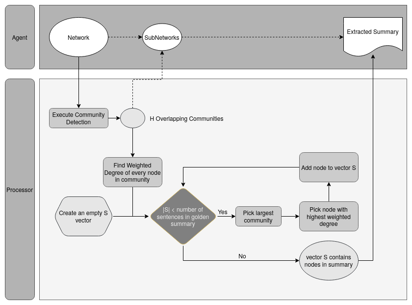
Figure 3. Flow diagram showing extraction of most important sentences in the document using propose CoRank method

5. Explanation of the proposed methodology using example network

To further illustrate the process undertaken by the algorithm, a graph $G=(V,E)$ is taken as given in figure 4. To assign the weights to this example network, degree of the nodes is calculated. A parameter $\theta=\frac{E}{V}$ is used as threshold. For every link, if either of nodes have a degree greater than $\theta$, weight is drawn from a random number generator (between 2 and 10), available through the random package in python 3, otherwise the degree is set to unity. The weight of each link for the example network thus found is mentioned in the table 1. Table 2 presents the index mapping of the edges of the example network given in figure 4.

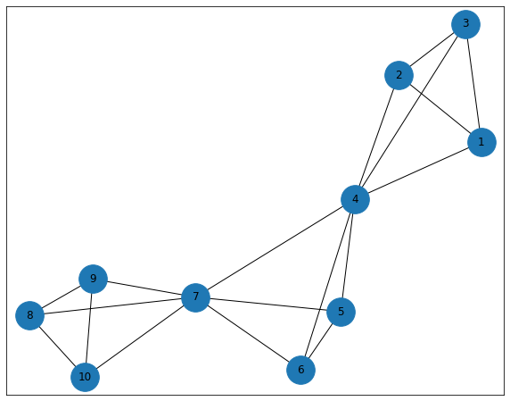
Figure 4. Flow diagram showing detection of communities by the algorithm.

Table 1. Weights of the edges in the example graph(given in Fig.4)

Edge	Weight	Edge	Weight	Edge	Weight	Edge	Weight
(1, 2)	9	(1, 3)	6	(1, 4)	5	(2, 3)	7
(2, 4)	2	(3, 4)	5	(4, 5)	2	(4, 6)	2
(4, 7)	5	(5, 6)	2	(5, 7)	8	(6, 7)	5
(7, 8)	9	(7, 9)	3	(7, 10)	9	(8, 9)	2
(8, 10)	4	(9, 10)	6	-	-	-	-

Table 2. Index Mapping of the edges in the example graph(given in Fig.4)

Edge	Map Index	Edge	Map Index	Edge	Map Index	Edge	Map Index
(1, 2)	1	(1, 3)	2	(1, 4)	3	(2, 3)	4
(2, 4)	5	(3, 4)	6	(4, 5)	7	(4, 6)	8
(4, 7)	9	(5, 6)	10	(5, 7)	11	(6, 7)	12
(7, 8)	13	(7, 9)	14	(7, 10)	15	(8, 9)	16
(8, 10)	17	(9, 10)	18	-	-	-	-

5.1. Part A: Community Detection

5.1.1. Step 1: Find First Order Approximate Neighbors (FOAN)

FOAN of every edge in the network is calculated using the equation 1. The table 3 shows the calculated FOAN for the example network given in Fig.4.

Edge	Elements in FOAN (Edge Map Indices)
(1, 2)	1, 2, 3, 4, 5
(1, 3)	1, 2, 3, 4, 6
(1, 4)	1, 2, 3, 5, 6, 7, 8, 9
(2, 3)	1, 2, 4, 5, 6
(2, 4)	1, 3, 4, 5, 6, 7, 8, 9
(3, 4)	2, 3, 4, 5, 6, 7, 8, 9
(4, 5)	3, 5, 6, 7, 8, 9, 10, 11
(4, 6)	3, 5, 6, 7, 8, 9, 10, 12
(4, 7)	3, 5, 6, 7, 8, 9, 11, 12, 13, 14, 15
(5, 6)	7, 8, 10, 11, 12
(5, 7)	7, 9, 10, 11, 12, 13, 14, 15
(6, 7)	8, 9, 10, 11, 12, 13, 14, 15
(7, 8)	9, 11, 12, 13, 14, 15, 16, 17
(7, 9)	9, 11, 12, 13, 14, 15, 16, 18
(7, 10)	9, 11, 12, 13, 14, 15, 17, 18
(8, 9)	13, 14, 16, 17, 18
(8, 10)	13, 15, 16, 17, 18
(9, 10)	14, 15, 16, 17, 18

Table 3. FOAN of all edges in graph. The numbers shown in right column are the edge map indices for brevity, refer to table 2.

5.1.2. Step 2: Find Second Order Approximate Neighbors (SOAN)

SOAN of every edge in the network is calculated using the equation 2. The table 4 shows the calculated FOAN for the example network(given in Fig.4).

Edge	Elements in SOAN (Edge Map Indices)
(1, 2)	1, 2, 3, 4, 5
(1, 3)	1, 2, 3, 4, 6
(1, 4)	1, 2, 3, 5, 6, 7, 8, 9
(2, 3)	1, 2, 4, 5, 6
(2, 4)	1, 3, 4, 5, 6, 7, 8, 9
(3, 4)	2, 3, 4, 5, 6, 7, 8, 9
(4, 5)	3, 5, 6, 7, 8, 9, 10, 11
(4, 6)	3, 5, 6, 7, 8, 9, 10, 12
(4, 7)	3, 5, 6, 7, 8, 9, 11, 12, 13, 14, 15
(5, 6)	7, 8, 10, 11, 12
(5, 7)	7, 9, 10, 11, 12, 13, 14, 15
(6, 7)	8, 9, 10, 11, 12, 13, 14, 15
(7, 8)	9, 11, 12, 13, 14, 15, 16, 17
(7, 9)	9, 11, 12, 13, 14, 15, 16, 18
(7, 10)	9, 11, 12, 13, 14, 15, 17, 18
(8, 9)	13, 14, 16, 17, 18
(8, 10)	13, 15, 16, 17, 18
(9, 10)	14, 15, 16, 17, 18

Table 4. SOAN of all edges in graph. The numbers shown in right column are the edge map indices for brevity, refer to table 2.

5.1.3. Step 3: Find Jaccard Similarity

For every pair of $F(e_{i,j})$ corresponding vectors $\overline{e}_{i,j}$ are calculated and Jaccard similarity is found out using the equation 3. The Jaccard Similarity for the given example graph(shown in Fig.4) is given in table 5.

	1	2	3	4	5	6	7	8	9	10	11	12	13	14	15	16	17	18
1	$\infty$
2	0.79	$\infty$
3	0.51	0.58	$\infty$
4	0.71	0.79	0.51	$\infty$
5	0.53	0.60	0.70	0.53	$\infty$
6	0.47	0.53	0.63	0.47	0.65	$\infty$
7	0.13	0.19	0.46	0.13	0.45	0.48	$\infty$
8	0.14	0.20	0.49	0.14	0.48	0.51	0.64	$\infty$
9	0.09	0.13	0.30	0.09	0.30	0.31	0.51	0.46	$\infty$
10	0.00	0.00	0.08	0.00	0.08	0.08	0.39	0.31	0.30	$\infty$
11	0.00	0.00	0.10	0.00	0.10	0.10	0.30	0.25	0.72	0.38	$\infty$
12	0.00	0.00	0.10	0.00	0.10	0.10	0.30	0.25	0.72	0.38	0.91	$\infty$
13	0.00	0.00	0.07	0.00	0.06	0.07	0.21	0.16	0.64	0.25	0.80	0.80	$\infty$
14	0.00	0.00	0.06	0.00	0.06	0.07	0.20	0.15	0.62	0.25	0.76	0.76	0.80	$\infty$
15	0.00	0.00	0.06	0.00	0.06	0.06	0.19	0.15	0.60	0.24	0.74	0.74	0.84	0.88	$\infty$
16	0.00	0.00	0.00	0.00	0.00	0.00	0.00	0.00	0.18	0.00	0.22	0.22	0.35	0.39	0.43	$\infty$
17	0.00	0.00	0.00	0.00	0.00	0.00	0.00	0.00	0.27	0.00	0.33	0.33	0.47	0.51	0.55	0.64	$\infty$
18	0.00	0.00	0.00	0.00	0.00	0.00	0.00	0.00	0.18	0.00	0.22	0.22	0.35	0.39	0.43	0.45	0.64	$\infty$

Table 5. Jaccard Similarity

5.1.4. Step 4: Find Constrained Second Order Approximate Neighbors

The algorithm uses the Jaccard Similarity found in the previous step to eliminate weaker relations in SOAN. Using a threshold $\delta_{cson}=0.5$ and $\alpha^{t=1}_{decay}=0.8$, CSON (table 6 is found. This completes the first iteration. The CSON acts as FOAN for the next iteration. The loop stops when $CSON_{new}$ is same as $CSON_{prev}$.

Edge	Elements in CSOAN (Edge Map Indices)
(1, 2)	1, 2, 3, 4, 5
(1, 3)	1, 2, 3, 4, 5, 6
(1, 4)	1, 2, 3, 4, 5, 6
(2, 3)	1, 2, 3, 4, 5
(2, 4)	1, 2, 3, 4, 5, 6
(3, 4)	2, 3, 5, 6, 8
(4, 5)	7, 8, 9
(4, 6)	6, 7, 8
(4, 7)	7, 9, 11, 12, 13, 14, 15
(5, 6)	10
(5, 7)	9, 11, 12, 13, 14, 15
(6, 7)	9, 11, 12, 13, 14, 15
(7, 8)	9, 11, 12, 13, 14, 15
(7, 9)	9, 11, 12, 13, 14, 15, 17
(7, 10)	9, 11, 12, 13, 14, 15, 17
(8, 9)	16, 17
(8, 10)	14, 15, 16, 17, 18
(9, 10)	17, 18

Table 6. CSOAN of all edges in graph. The numbers shown in right column are the edge map indices for brevity, refer to table 2.

5.1.5. Step 5: Merging Link Node Sets (LNS)

After 4 iterations, a stable set of CSON is formed. The CSOAN of each edge does not change in any further iteration. CSON are converted into LNS - Link Node Set using equation 5. For every set of LNS, conductance is calculated and two LNS are merged (union) if and only if the resultant set has a lower conductance than the individual values. The values of stable CSON, LNS and their conductance is given in table 7.

Edge	Elements in CSOAN (Edge Map Indices)	Link Node Set	Conductance $\phi$
(1, 2)	1, 2, 3, 4, 5, 6	3, 4, 1, 2	0.2
(1, 3)	1, 2, 3, 4, 5, 6	3, 4, 1, 2	0.2
(1, 4)	1, 2, 3, 4, 5, 6	3, 4, 1, 2	0.2
(2, 3)	1, 2, 3, 4, 5, 6	3, 4, 1, 2	0.2
(2, 4)	1, 2, 3, 4, 5, 6	3, 4, 1, 2	0.2
(3, 4)	1, 2, 3, 4, 5, 6	3, 4, 1, 2	0.2
(4, 5)	7	4, 5	0.778
(4, 6)	8	4, 6	0.778
(4, 7)	9, 11, 12, 13, 14, 15	8, 6, 5, 10, 7, 4, 9	0.334
(5, 6)	10	6, 5	0.667
(5, 7)	9, 11, 12, 13, 14, 15	8, 6, 5, 10, 7, 4, 9	0.334
(6, 7)	9, 11, 12, 13, 14, 15	8, 6, 5, 10, 7, 4, 9	0.334
(7, 8)	9, 11, 12, 13, 14, 15	8, 6, 5, 10, 7, 4, 9	0.334
(7, 9)	9, 11, 12, 13, 14, 15	8, 6, 5, 10, 7, 4, 9	0.334
(7, 10)	9, 11, 12, 13, 14, 15	8, 6, 5, 10, 7, 4, 9	0.334
(8, 9)	16	8, 9	0.667
(8, 10)	17, 18	8, 10, 9	0.334
(9, 10)	17, 18	8, 10, 9	0.334

Table 7. CSOAN of all edges in graph after the loop stops. The numbers shown in right column are the edge map indices for brevity, refer to table 2.

After merging the LNS, the communities thus found are given in table 8.

Communities Detected
1, 2, 3, 4	1, 2, 3, 4, 5, 6	4, 5, 6, 7, 8, 9, 10	1, 2, 3, 4, 8, 9, 10	8, 9, 10

Table 8. Communities Detected

5.2. Finding Influential Nodes / Important Sentences

After steps in section 5.1.5, a list of nodes in different communities is obtained. The overlapping communities are sorted in their decreasing length and the largest community is picked. In the given example $H=\{1,2,3,4,8,9,10\}$ is largest. The weighted degree of the nodes are found out as given in table 9. Node $1$ has highest degree, it is removed from the community and added to a vector $S$. $S$ now contains $S={1}$. Again the largest community is picked and found out to be $H=\{4,5,6,7,8,9,10\}$, node $10$ has highest weighted degree of $7$, it is added to vector $S$. $Snowcontains{1,7}$. Similarly, the operation is carried out till 5 nodes are found out. The resultant vector $S=\{1,7,3,10,2\}$. These are the most influential nodes in the network.

Node	Weighted Degree	Node	Weighted Degree	Node	Weighted Degree
1	20	2	18	3	18
4	12	8	6	9	8
		10	10

Table 9. Weighted degree of the nodes in community $H=\{1,2,3,4,8,9,10\}$

5.3. Complexity of proposed CoRank

For a graph $G=(V,E)$ where $V$ is the set of vertices and $E$ is the set of edges, complexity is computed of the proposed CoRank algorithm.

1. Community Detection -

   1. Computing FOAN: $O(|E|)$

   2. Computing SOAN: $O(|E|^{2})$

   3. Finding Jaccard Similarity: $O(|E|^{2}\cdot log(\overline{E}))$ where $\overline{E}$ represent average number of edges in FOAN.

   4. Computing CSON: $O(|E|^{2})$

   5. Merging LNS: $O(|E|\cdot log(m))$ where $m$ is the average number of LNS merged.

   This results in complexity of $O(|E|)+N_{iter}\cdot(O(|E|^{2})+O(|E|^{2}\cdot log(\overline{E}))+O(|E|\cdot log(m))$ where $N_{iter}$ is the number of iterations performed to obtain a stable CSOAN, equivalent to $N_{iter}O(|E|^{2}\cdot log(\overline{E}))$. The maximum number of iterations the algorithm will be at most $|E|$. This gives a upper bound on the complexity of this step as $O(|E|^{3})$.

2. Influential Nodes - For $g$ number of sentences in the golden summary, this step takes $g\cdot O(|V|^{2})$. This is a poor upper bound as the number of edges formed during graph construction are far fewer than $\binom{|V|}{2}$ and this step takes very few seconds on real test cases.

3. Thus, the complexity of proposed CoRank is $O(|E|^{3})+O(|V|^{2})$

5.4. Real Examples

Given a document with text as given in figure 5.4, the algorithm is used to perform the extractive summarization. It detects $|\mathcal{H}|=23$ communities and the sentences mentioned in quotes below are extracted. ROUGE-n gram score is computed to analyse the efficacy of the extracted summary(a brief discussion about ROUGE is given in Section 6.3). The results obtained in terms of recall, precision, and f-score demonstrate the efficiency of the proposed approach.

Document:
Source: CNN News Article by Val Willingham
A debilitating, mosquito-borne virus called chikungunya has made its way to North Carolina, health officials say. It’s the state’s first reported case of the virus. The patient was likely infected in the Caribbean, according to the Forsyth County Department of Public Health. Chikungunya is primarily found in Africa, East Asia and the Caribbean islands, but the Centers for Disease Control and Prevention has been watching the virus,+ for fear that it could take hold in the United States – much like West Nile did more than a decade ago. The virus, which can cause joint pain and arthritis-like symptoms, has been on the U.S. public health radar for some time. About 25 to 28 infected travelers bring it to the United States each year, said Roger Nasci, chief of the CDC’s Arboviral Disease Branch in the Division of Vector-Borne Diseases. ”We haven’t had any locally transmitted cases in the U.S. thus far,” Nasci said. But a major outbreak in the Caribbean this year – with more than 100,000 cases reported – has health officials concerned. Experts say American tourists are bringing chikungunya back home, and it’s just a matter of time before it starts to spread within the United States. Study: Beer drinkers attract mosquitoes

Study: Beer drinkers attract mosquitoes 01:26 After all, the Caribbean is a popular one with American tourists, and summer is fast approaching. ”So far this year we’ve recorded eight travel-associated cases, and seven of them have come from countries in the Caribbean where we know the virus is being transmitted,” Nasci said. Other states have also reported cases of chikungunya. The Tennessee Department of Health said the state has had multiple cases of the virus in people who have traveled to the Caribbean. The virus is not deadly, but it can be painful, with symptoms lasting for weeks. Those with weak immune systems, such as the elderly, are more likely to suffer from the virus’ side effects than those who are healthier. The good news, said Dr. William Shaffner, an infectious disease expert with Vanderbilt University in Nashville, is that the United States is more sophisticated when it comes to controlling mosquitoes than many other nations. ”We live in a largely air-conditioned environment, and we have a lot of screening (window screens, porch screens),” Shaffner said. ”So we can separate the humans from the mosquito population, but we cannot be completely be isolated.” Chikungunya was originally identified in East Africa in the 1950s. The ecological makeup of the United States supports the spread of an illness such as this, especially in the tropical areas of Florida and other Southern states, according to the CDC. The other concern is the type of mosquito that carries the illness. Unlike most mosquitoes that breed and prosper outside from dusk to dawn, the chikungunya virus is most often spread to people by Aedes aegypti and Aedes albopictus mosquitoes. These are the same mosquitoes that transmit the virus that causes dengue fever. They bite mostly during the daytime. The disease is transmitted from mosquito to human, human to mosquito and so forth. A female mosquito of this type lives three to four weeks and can bite someone every three to four days.

Extracted: Chikungunya is primarily found in Africa, East Asia and the Caribbean islands, but the Centers for Disease Control and Prevention has been watching the virus,+ for fear that it could take hold in the United States much like West Nile did more than a decade ago. Experts say American tourists are bringing chikungunya back home, and it’s just a matter of time before it starts to spread within the United States. The virus, which can cause joint pain and arthritis-like symptoms, has been on the U.S. public health radar for some time.
Golden Summary: North Carolina reports first case of mosquito-borne virus called chikungunya. Chikungunya is primarily found in Africa, East Asia and the Caribbean islands. Virus is not deadly, but it can be painful, with symptoms lasting for weeks.

	Recall	Precision	F1-score
ROUGE-1	0.824034	0.64646465	0.72452830
ROUGE-2	0.517241	0.40540541	0.45454545
ROUGE-3	0.246753	0.19322034	0.21673004

Table 10. ROUGE-1, 2, 3 score on the given real example in Subsection 5.4

6. Analysis of Experiments

To validate the efficiency of the proposed approach, experiments are conducted on the data sets given by Document Understanding Conference (DUC). DUC is a method assessment competition that allows researchers to assess the efficiency of various summarization methods on similar data sets.

Table 11. Statistics of Data sets

	DUC 2001	DUC 2002
Count of clusters	30	59
Length of summary	100 words	100 words
Source of data	TREC-9	TREC-9
Count of documents	309	567

6.1. Data sets

A brief description about the statistics of the data set is presented in Table 10. DUC 2001 and DUC 2002 data set is used for experimental analysis and a comparative study is made for the system generated summaries and golden summaries.

6.2. Pre-processing

Some linguistic techniques such as stemming, upper case removal, removal of stop words, and segmentation of sentences has been used during pre-processing phase of the document in this experiment. The textual content of the document is divided into sentences during the process of segmentation. Words appearing frequently such as a, an, the etc. within the text are removed during stop word removal process, since they are considered irrelevant. The process of stemming involves reduction of a word to its root stem. PorterStemmer is used for the stemming of word. The process of pre-processing is performed before the execution of the algorithm.

6.3. Evaluation Metric

DUC has adopted ROUGE metric (Lin, 2004) for evaluation of automatically generated summary, hence, the proposed research uses this metric for performance analysis of the proposed research. The quality of summary is measured using ROUGE metric, that basically counts the number of overlapping units such as word pairs, word sequences, and n-grams between the reference summary and candidate summary. ROUGE-1 and ROUGE-2 recall score is used in this research for the evaluation of automatic summaries.

6.4. Evaluation of performance

Methods	DUC01				DUC02
	R-1	Rank	R-2	Rank	R-1	Rank	R-2	Rank
FEOM	0.4773	1	0.1855	5	0.4658	7	0.1249	8
CoRank	0.4725	2	0.2011	2	0.4906	1	0.2306	1
NetSum	0.4643	3	0.1770	7	0.4496	8	0.1117	9
CRF	0.4551	4	0.1773	9	0.4401	10	0.1092	10
ESDS	0.4540	5	0.1957	4	0.4790	5	0.2214	4
UnifiedRank	0.4538	6	0.1765	8	0.4849	2	0.2146	5
MA	0.4486	7	0.2014	1	0.4828	3	0.2284	3
QCS	0.4485	8	0.1852	6	0.4487	9	0.1877	7
LexRank	0.4468	9	0.1989	3	0.4796	4	0.2295	2
SVM	0.4463	10	0.1702	10	0.4324	11	0.1087	11
CollabSum	0.4404	11	0.1623	12	0.4719	6	0.2010	6
ManifoldRanking	0.4336	12	0.1664	11	0.4233	12	0.1068	12
DPSO	0.3993	13	0.0832	13	0.4172	13	0.1026	13
0-1 non-linear	0.0.3876	14	0.0778	14	0.4097	14	0.0937	14

Table 12. R-1 and R-2 recall score for DUC01 and DUC02 dataset

This section deals with a comparative analysis of the performance of the proposed approach with some recent works. The proposed CoRank method is compared with some baseline methods: (a) ESDS (Mendoza et al., 2015) – a search algorithm based on binary optimization, (b) manifold ranking (Wan et al., 007a)- greedy search involving probabilistic approach, (c) NetSum (Svore et al., 2007) - approach based on neural networks, (d) MA (Mendoza et al., 2014a)- local search and genetic operators based metaheuristic approach, (e) CRF (Shen et al., 2007)- approach based on conditional random field, (f) FEOM (Song et al., 2014) – evolutionary algorithm involving fuzzy approach, (g) SVM (Yeh et al., 2005) - mathematical approach, (h) QC (Dunlavy et al., 2007) - hidden markov model based approach, (i) 0–1 non linear (Alguliev et al., 2013) - evolutionary algorithm approach based on binary PSO, (j) UnifiedRank (Wan, 2010) - ranking approach based on graph, (k) CollabSum (Alguliev et al., 2007) - clustering approach along with ranking of graphs, (l) LexRank (Erkan and Radev, 2004) - method involving ranking of graphs, (m) DPSO (Alguliev et al., 011a) - optimization approach based on evolutionary algorithm. The above methods have accomplished good results on DUC01 and DUC02 data sets, due to this reason they are selected for comarison with the proposed CoRank method.

Table 11 presents R-1 and R-2 recall score for DUC01 and DUC02 data sets. As is concerned for DUC01 data set, FEOM and CoRank acheive first and second place for R-1 recall score, whereas MA and CoRank accomplish first and second place for R-2 recall score. For DUC02 data set, Corank is performing best for both R-1 and R-2 recall score, with DPSO and 0-1 non-linear performing worst in every case.

Methods	DUC01		DUC02
	R-1	R-2	R-1	R-2
FEOM	(-)0.96	(+) 8.46	(+) 5.37	(+) 84.87
NetSum	(+)1.81	(+) 13.67	(+) 9.16	(+) 106.71
CRF	(+)3.87	(+) 16.10	(+) 11.52	(+) 111.45
ESDS	(+)4.12	(+) 2.81	(+) 2.46	(+) 4.29
UnifiedRank	(+)4.16	(+) 13.99	(+) 1.22	(+) 7.60
MA	(+)5.37	(-) 0.10	(+) 1.66	(+) 1.09
QCS	(+)5.40	(+) 8.64	(+) 9.38	(+) 23.02
LexRank	(+)5.80	(+) 1.16	(+) 2.34	(+) 0.61
SVM	(+)5.92	(+) 18.21	(+) 13.51	(+) 112.42
CollabSum	(+)7.33	(+) 23.97	(+) 4.01	(+) 14.88
ManifoldRanking	(+)9.02	(+) 20.91	(+) 15.95	(+) 116.20
DPSO	(+)18.38	(+) 141.83	(+) 17.64	(+) 125.05
0-1 non-linear	(+)21.96	(+) 158.61	(+) 19.79	(+) 146.42

Table 13. Relative improvement of CoRank with other methods

A significant improvement was observed in the performance of the proposed approach for R-1 and R-2 recall score in comparison with other methods. The relative improvement of CoRank wrt other approaches is presented in Table 12. As is evident, CoRank outperforms state-of-the-art methods and achieves highest R-1 and R-2 recall score for DUC01 and DUC02 data sets. Relative improvement is used as a measure for comparison. The formula for calculating relative improvement is (c-b)*100/b, where a comparison of c is made with a. For showing the relative improvement of CoRank with other methods “+” sign is used, whereas “-” means opposite. As shown in Table 12, CoRank has outperformed other methods for R-1 and R-2 recall score on DCU01 and DUC02 data sets. For DUC01 data set, only FEOM and MA have performed better than CoRank. FEOM has shown an improvement of 0.96% for R-1 metric whereas, MA is performing 0.10% better than CoRank for R-2 metric. CoRank has outperformed state-of-the-art methods for DUC02 dataset. The reason for CoRank’s good performance is, it is clustering sentences based on large sub-topics that are carrying more weight, and obtained salient sentences have maximum diversity and coverage.

Based on Table 12 observation, we can draw following conclusion:

• The proposed approach CoRank has outperformed state-of-the-art-methods for DUC02 data set and performed competitively well for DUC01 data set except for DE and MA method.

• Although LexRank and UnifiedRank are graph based approaches, but its performance is less in comparison to CoRank, which is a combination of clustering and graph ranking method.

• CoRank, FEOM, UnifiedRank, ESDS, LexRank, and MA are unsupervised methods that have performed better than SVM , a supervised approach.

• 0-1 non-linear and DPSO have failed to perform, since they don’t use clustering concept.

• Following conclusion is drawn when CoRank is compared with FEOM, MA, and NetSum, the top performing methods:(a) combination of graph based approaches with clustering has a bright future for further research in the domain of extractive summarization.

7. Conclusion

This research work proposes CoRank: a clustering combined graph ranking approach for generating extractive summaries. It aims to cover two aspects: (a) diversity – obtained summary should not cover redundant information; (b) coverage – resultant summary should contain different main topics , sub-topics of the oringinal source document. Initially, a clustering algorithm is proposed that groups sentences into clusters based on topics and sub-topics. Then, from every cluster, most salient and representative sentences are selected using proposed CoRank algorithm.

The preformance of the CoRank algorithm is validated on DUC01 and DUC02 datasets in terms of Recall-1 and Recall-2 measure. The proposed approach obtains best results for DUC02 dataset beating the best performing MA approach by 1.66% and 1.09% . It obtains good results for DUC01 dataset, however, slightly lagging behind FEOM approach. Other graph based approaches such as LexRank and UnifiedRanking are not so effective since they lack the concept of clustering. The reason for the promising results of the proposed CoRank approach is, it is able to extract main topics and sub-topics from the main text with maximum coverage and diversity.

The future work remains to include more techniques based on optimization, and use different combination of similarity measures for extracting summaries.

References

- (1)
- Ahmad et al. (2020) Amreen Ahmad, Tanvir Ahmad, and Abhishek Bhatt. 2020. HWSMCB: A community-based hybrid approach for identifying influential nodes in the social network. Physica A: Statistical Mechanics and its Applications 545 (may 2020), 123590. https://doi.org/10.1016/j.physa.2019.123590
- Alguliev et al. (2012) Rasim M. Alguliev, Ramiz M. Aliguliyev, and Nijat R. Isazade. 2012. DESAMC+DocSum: Differential Evolution with Self-Adaptive Mutation and Crossover Parameters for Multi-Document Summarization. 36 (2012).
- Alguliev et al. (2007) R. M. Alguliev, R. M. Aliguliyev, and C. A. Mehdiyev. 2007. CollabSum: exploiting multiple document clustering for collaborative single document summarizations. Proceedings of the 30th Annual International ACM SIGIR Conference on Research and Development in Information Retrieval (2007), 143–150.
- Alguliev et al. (011a) R. M. Alguliev, R. M. Aliguliyev, and C. A. Mehdiyev. 2011a. An optimization model and DPSO‐EDA for document summarization. International Journal of Information Technology and Computer Science 3(5) (2011a), 59–68.
- Alguliev et al. (2013) R. M. Alguliev, R. M. Aliguliyev, and C. A. Mehdiyev. 2013. An optimization approach to automatic generic document summarization. Computational Intelligence 29(1) (2013), 129–155.
- Alguliyev et al. (2017) R. Alguliyev, R. Aliguliyev, Nijat R. Isazade, Asad Abdi, and Norisma Idris. 2017. A Model for Text Summarization. Int. J. Intell. Inf. Technol. 13 (2017), 67–85.
- Anam et al. (2018) Shakil Ashraful Anam, A M Muntasir Rahman, Nasif Noor Saleheen, and Hossain Arif. 2018. Automatic Text Summarization using Fuzzy C-Means Clustering. In 2018 Joint 7th International Conference on Informatics, Electronics Vision (ICIEV) and 2018 2nd International Conference on Imaging, Vision Pattern Recognition (icIVPR). 180–184. https://doi.org/10.1109/ICIEV.2018.8641055
- Balaji et al. (2014) J Balaji, T V Geetha, and Ranjani Parthasarathi. 2014. A Graph Based Query Focused Multi-Document Summarization. 10, 1 (2014).
- Batista et al. (2016) Jamilson Batista, Rafael Dueire Lins, Rinaldo Lima, Steven J. Simske, and Marcelo Riss. 2016. Towards cohesive extractive summarization through anaphoric expression resolution. In DocEng 2016 - Proceedings of the 2016 ACM Symposium on Document Engineering. Association for Computing Machinery, Inc, 201–204. https://doi.org/10.1145/2960811.2967159
- Begum et al. (2009) Nadira Begum, Mohamed Fattah, and Fuji Ren. 2009. Automatic text summarization using support vector machine. International Journal of Innovative Computing, Information and Control 5 (07 2009), 1987–1996.
- Bonzanini et al. (2013) Marco Bonzanini, Miguel Martinez-Alvarez, and Thomas Roelleke. 2013. Extractive summarisation via sentence removal: Condensing relevant sentences into a short summary. 893–896 pages. https://doi.org/10.1145/2484028.2484149
- Cai and Li (2011) Xiaoyan Cai and Wenjie Li. 2011. A spectral analysis approach to document summarization: Clustering and ranking sentences simultaneously. Information Sciences 181, 18 (2011), 3816–3827.
- Cai et al. (2014a) Xiaoyan Cai, Wenjie Li, and Renxian Zhang. 2014a. Combining Co-Clustering with Noise Detection for Theme-Based Summarization. 10, 4 (2014).
- Cai et al. (2014b) Xiaoyan Cai, Wenjie Li, and Renxian Zhang. 2014b. Enhancing diversity and coverage of document summaries through subspace clustering and clustering-based optimization. Information Sciences 279 (2014), 764–775.
- Chali et al. (2009) Yllias Chali, Sadid A. Hasan, and Shafiq R. Joty. 2009. A SVM-Based Ensemble Approach to Multi-Document Summarization. In Proceedings of the 22nd Canadian Conference on Artificial Intelligence: Advances in Artificial Intelligence (Kelowna, Canada) (Canadian AI ’09). Springer-Verlag, Berlin, Heidelberg, 199–202. https://doi.org/10.1007/978-3-642-01818-3_23
- Dhillon et al. (2001) I. Dhillon, S. Mallela, and S. Modha. 2001. Information-theoretic co-clustering. In Proceedings of ACM (SIGKDD) International Conference on Knowledge Discovery and Data Mining (2001), 89–98.
- Ding et al. (2016) Zhuanlian Ding, Xingyi Zhang, Dengdi Sun, and Bin Luo. 2016. Overlapping Community Detection based on Network Decomposition. Scientific Reports 6, 1 (apr 2016), 1–11. https://doi.org/10.1038/srep24115
- Duda et al. (2001) R. Duda, P. Hart, and D. Stork. 2001. Pattern Classification. (2001).
- Dunlavy et al. (2007) D. M. Dunlavy, D. P. O’leary, J. M. Conroy, and J. D. Schlesinger. 2007. QCS: A system for querying, clustering and summarizing documents. Information Processing & Management 43(15) (2007), 1588–1605.
- Erkan and Radev (2004) G. Erkan and D. Radev. 2004. LexRank: Graph‐based centrality as salience in text summarization. Journal of Artificial Intelligence Research 22 (2004), 457–479.
- Ferreira et al. (2014) Rafael Ferreira, Luciano Cabral, Fred Freitas, Rafael Lins, Gabriel Silva, Steven Simske, and Luciano Favaro. 2014. A multi-document summarization system based on statistics and linguistic treatment. Expert Systems with Applications 41 (10 2014), 5780–5787. https://doi.org/10.1016/j.eswa.2014.03.023
- Gupta and Kumar (2020) Samrat Gupta and Pradeep Kumar. 2020. An overlapping community detection algorithm based on rough clustering of links. Data and Knowledge Engineering 125 (jan 2020), 101777. https://doi.org/10.1016/j.datak.2019.101777
- Hingu et al. (2015) Dharmendra Hingu, Deep Shah, and Sandeep S. Udmale. 2015. Automatic text summarization of Wikipedia articles. In 2015 International Conference on Communication, Information Computing Technology (ICCICT). 1–4. https://doi.org/10.1109/ICCICT.2015.7045732
- Jang and Kang (2021) Myeongjun Jang and Pilsung Kang. 2021. Learning-Free Unsupervised Extractive Summarization Model. IEEE Access 9 (2021), 14358–14368. https://doi.org/10.1109/ACCESS.2021.3051237
- Jing and Mckeown (2000) H. Jing and K. Mckeown. 2000. Cut and paste based text summarization. In Proceedings of the Annual Conference of the North American Chapter of the Association for Computational Linguistics (NAACL) (2000).
- Knight and Marcu (2002) K. Knight and D. Marcu. 2002. Summarization beyond sentence extraction: A probablistic approach to sentence compression. Artificial Intell. (2002).
- Li and Li (2014) Yanran Li and Sujian Li. 2014. Query-focused Multi-Document Summarization: Combining a Topic Model with Graph-based Semi-supervised Learning. In Proceedings of COLING 2014, the 25th International Conference on Computational Linguistics: Technical Papers. Dublin City University and Association for Computational Linguistics, Dublin, Ireland, 1197–1207. https://www.aclweb.org/anthology/C14-1113
- Lin (2004) C.‐Y. Lin. 2004. Rouge: A package for automatic evaluation of summaries. In Proceedings of the Workshop on Text Summarization Branches Out (2004), 74–81.
- LLORET and Sanz (2013) ELENA LLORET and Manuel Sanz. 2013. COMPENDIUM: A text summarisation tool for generating summaries of multiple purposes, domains, and genres. Natural Language Engineering 19 (04 2013). https://doi.org/10.1017/S1351324912000198
- Luo et al. (2013) Wenjuan Luo, Fuzhen Zhuang, Qing He, and Zhongzhi Shi. 2013. Exploiting Relevance, Coverage, and Novelty for Query-Focused Multi-Document Summarization. 46 (2013).
- Mani (2001) I. Mani. 2001. Automatic Summarization. John Benjamins Publishing Company (2001).
- Mei and Chen (2012) Jian-Ping Mei and Lihui Chen. 2012. SumCR: A new subtopic-based extractive approach for text summarization. Knowledge and Information Systems - KAIS 31 (06 2012). https://doi.org/10.1007/s10115-011-0437-x
- Mendoza et al. (2014a) M. Mendoza, S. Bonilla, C. Noguera, C. Cobos, and E. León. 2014a. Extractive single‐document summarization based on genetic operators and guided local search. Expert Systems with Applications 41(9) (2014), 4158–4169.
- Mendoza et al. (2014b) Martha Mendoza, Susana Bonilla, Clara Noguera, C. Lozada, and E. Guzman. 2014b. Extractive single-document summarization based on genetic operators and guided local search. Expert Syst. Appl. 41 (2014), 4158–4169.
- Mendoza et al. (2015) M. Mendoza, C. Cobos, and E. León. 2015. Extractive single‐document summarization based on global‐best harmony search and a greedy local optimizer. Lecture Notes in Artificial Intelligence 9414 (2015), 52–66.
- Nishino et al. (2013) Masaaki Nishino, Norihito Yasuda, Hirao Tsutomu, Jun Suzuki, and Masaaki Nagata. 2013. Lagrangian Relaxation for Scalable Text Summarization while Maximizing MultipleObjectives. Transactions of the Japanese Society for Artificial Intelligence 28 (07 2013), 433–441. https://doi.org/10.1527/tjsai.28.433
- Ozsoy et al. (2011) Makbule Ozsoy, Ferda Alpaslan, and Ilyas Cicekli. 2011. Text summarization using Latent Semantic Analysis. J. Information Science 37 (08 2011), 405–417. https://doi.org/10.1177/0165551511408848
- Parveen et al. (2015) Daraksha Parveen, Hans-Martin Ramsl, and Michael Strube. 2015. Topical Coherence for Graph-based Extractive Summarization. In Proceedings of the 2015 Conference on Empirical Methods in Natural Language Processing. Association for Computational Linguistics, Lisbon, Portugal, 1949–1954. https://doi.org/10.18653/v1/D15-1226
- Ricardo and Berthier (1999) B. Ricardo and R. Berthier. 1999. Modern Information Retrieval. ACM Press (1999).
- Shen et al. (2007) D. Shen, J.‐T. Sun, H Li, Q. Yang, and Z. Chen. 2007. Document summarization using conditional random fields. In Proceedings of the 20th International Joint Conference on Artificial Intelligence (2007), 2862–2867.
- Shetty and Kallimani (2017) Krithi Shetty and Jagadish S. Kallimani. 2017. Automatic extractive text summarization using K-means clustering. In 2017 International Conference on Electrical, Electronics, Communication, Computer, and Optimization Techniques (ICEECCOT). 1–9. https://doi.org/10.1109/ICEECCOT.2017.8284627
- Sonawane et al. (2019) Sheetal Sonawane, Parag Kulkarni, Charusheela Deshpande, and Bhagyashree Athawale. 2019. Extractive summarization using semigraph (ESSg). Evolving Systems 10, 3 (sep 2019), 409–424. https://doi.org/10.1007/s12530-018-9246-8
- Song et al. (2014) W. Song, J. Z. Liang, and S. C. Park. 2014. Fuzzy control GA with a novel hybrid semantic similarity strategy for text clustering. Information Sciences 273 (2014), 156–170.
- Svore et al. (2007) K. M. Svore, L. Vanderwende, and C. J. Burges. 2007. Enhancing single‐document summarization by combining RankNet and third‐party sources. Proceedings of the Joint Conference on Empirical Methods in Natural Language Processing and Computational Natural Language Learning (EMNLP‐CoNLL) (2007), 448–457.
- Turpin et al. (2007) A. Turpin, Y. Tsegay, D. Hawking, and H. Williams. 2007. Fast generation of result snippets in Web search. In Prodeedings of ACM SIGIR Conference on Research and Development on Information Retrieval (2007), 127–134.
- Wan (2010) Xiaojun Wan. 2010. Towards a Unified Approach to Simultaneous Single-Document and Multi-Document Summarizations. In Proceedings of the 23rd International Conference on Computational Linguistics (Coling 2010). Coling 2010 Organizing Committee, Beijing, China, 1137–1145. https://www.aclweb.org/anthology/C10-1128
- Wan et al. (007a) X. Wan, J. Yang, and J. Xiao. 2007a. Manifold‐ranking based topic‐focused multi‐document summarization. Proceedings of the 20th International Joint Conference on Artificial intelligence (2007a), 2903–2908.
- Yan and Guo (2020) Wanying Yan and Junjun Guo. 2020. Joint hierarchical semantic clipping and sentence extraction for document summarization. Journal of Information Processing Systems 16, 4 (aug 2020), 820–831. https://doi.org/10.3745/JIPS.04.0181
- Yang and Wang (2008) Christopher C. Yang and Fu Lee Wang. 2008. Hierarchical summarization of large documents. Journal of the American Society for Information Science and Technology 59, 6 (2008), 887–902. https://doi.org/10.1002/asi.20781
- Yang et al. (2018) Pingle Yang, Xin Liu, and Guiqiong Xu. 2018. A dynamic weighted TOPSIS method for identifying influential nodes in complex networks. Modern Physics Letters B 32, 19 (jul 2018). https://doi.org/10.1142/S0217984918502160
- Yeh et al. (2005) J.‐H. Yeh, H.‐R. Ke, W.‐P. Yang, and I.‐H. Meng. 2005. Text summarization using a trainable summarizer and latent semantic analysis. Information Processing & Management 41(1) (2005), 75–95.
- Zamir and Etzioni (1998) O. Zamir and O. Etzioni. 1998. Web document clustering: A feasibility demonstration. In Proceedings of ACM SIGIR Conference on Research and Development on Information Retrieval (1998), 46–54.
- Zhang et al. (2020) Zufan Zhang, Xieliang Li, and Chenquan Gan. 2020. Identifying influential nodes in social networks via community structure and influence distribution difference. Digital Communications and Networks (may 2020). https://doi.org/10.1016/j.dcan.2020.04.011
- Zopf et al. (2018) Markus Zopf, Eneldo Loza Mencía, and Johannes Fürnkranz. 2018. Which Scores to Predict in Sentence Regression for Text Summarization?. In Proceedings of the 2018 Conference of the North American Chapter of the Association for Computational Linguistics: Human Language Technologies, Volume 1 (Long Papers). Association for Computational Linguistics, New Orleans, Louisiana, 1782–1791. https://doi.org/10.18653/v1/N18-1161