A Unified Asymptotic Preserving and Well-balanced Scheme for the Euler System with Multiscale Relaxation

Abstract.

The design and analysis of a unified asymptotic preserving (AP) and well-balanced scheme for the Euler Equations with gravitational and frictional source terms is presented in this paper. The asymptotic behaviour of the Euler system in the limit of zero Mach and Froude numbers, and large friction is characterised by an additional scaling parameter. Depending on the values of this parameter, the Euler system relaxes towards a hyperbolic or a parabolic limit equation. Standard Implicit-Explicit Runge-Kutta schemes are incapable of switching between these asymptotic regimes. We propose a time semi-discretisation to obtain a unified scheme which is AP for the two different limits. A further reformulation of the semi-implicit scheme can be recast as a fully-explicit method in which the mass update contains both hyperbolic and parabolic fluxes. A space-time fully-discrete scheme is derived using a finite volume framework. A hydrostatic reconstruction strategy, an upwinding of the sources at the interfaces, and a careful choice of the central discretisation of the parabolic fluxes are used to achieve the well-balancing property for hydrostatic steady states. Results of several numerical case studies are presented to substantiate the theoretical claims and to verify the robustness of the scheme.

1. Introduction

Hyperbolic and kinetic equations with relaxation are ubiquitous in physical problems, such as in the theory of gases [13], non-equilibrium thermodynamics [14, 16], and linear and nonlinear waves [50], to name but a few. The main feature of relaxation problems is the occurrence of lower order terms in the governing equations, with respect to a small parameter $\varepsilon$ known as the relaxation parameter. The asymptotic limit $\varepsilon\to 0$ is often singular in the sense that the original governing equations of the problem approach a system of equations of a different mathematical and physical nature in the limit. A rigorous and systematic analysis of relaxation problems is due to Liu and collaborators [17, 37], which later lead to the development of the so-called relaxation schemes by Jin and Xin [32]. Depending on the particular scaling of the relaxation parameter $\varepsilon$, hyperbolic relaxation models can yield either hyperbolic or viscous conservation laws as their asymptotic limits. We refer the interested reader to, e.g. [2, 9, 38, 39] for a detailed analysis of relaxation systems. In [7], a new class of relaxation problems, termed as multiscale relaxation problems, is introduced wherein multiple scalings of the stiff terms are identified by various powers of the relaxation parameter $\varepsilon$ involving an exponent $\beta\in[0,1]$. When $\beta\in[0,1)$, the asymptotic limit of the relaxation system is hyperbolic in nature, and the limit $\varepsilon\to 0$ is known as hyperbolic-to-hyperbolic relaxation. On the other hand, $\beta=1$ gives a diffusion equation, and the corresponding limit is called hyperbolic-to-parabolic relaxation. In short, unlike standard relaxation systems, the asymptotic limit of a multiscale relaxation problem is also characterised by the scaling parameter $\beta$.

The numerical resolution of relaxation problems, or multiscale problems in general, poses a lot of difficulties. Standard explicit schemes work well in the macroscopic regime of the stiff relaxation parameter $(\varepsilon\sim 1)$ but in the microscopic regime $(\varepsilon\sim 0)$, these schemes encounter prohibitively expensive stability constraints. In addition, merely satisfying the stability constraints does not guarantee the accuracy of the scheme in the microscopic regime. It is well-known from literature, e.g. [26], that explicit time-stepping schemes suffer from a severe loss of accuracy in the stiff regime $\varepsilon\to 0$. Jin, in [27], introduced the notion of the so-called “Asymptotic Preserving (AP) schemes” in the context of kinetic models for transport in diffusive regimes, to tackle the multiscale nature of the problem and other associated difficulties. Formally, the basic idea behind an AP scheme can be explained in a general setting as follows. Let $\mathcal{P}_{\varepsilon}$ denote a singularly perturbed problem with $\varepsilon$, the perturbation parameter. Suppose that in the limit as $\varepsilon\to 0$, the solution of $\mathcal{P}_{\varepsilon}$ converges to the solution of a well-posed problem denoted by $\mathcal{P}_{0}$, called the singular limit or the limit problem. A numerical scheme for $\mathcal{P}_{\varepsilon}$, denoted by $\mathcal{P}_{\varepsilon}^{h}$ with $h$ being a discretisation parameter, is said to be asymptotic preserving if,

1. as $\varepsilon\to 0$ the numerical scheme $\mathcal{P}_{\varepsilon}^{h}$ converges to a numerical scheme $\mathcal{P}_{0}^{h}$, which is a consistent discretisation of the limit system $\mathcal{P}_{0}$, and

2. the stability constraints on the discretisation parameter $h$ are independent of $\varepsilon$.

Mathematically, the passage $\mathcal{P}_{\varepsilon}\to\mathcal{P}_{0}$ can often be formulated as a singular limit of the governing equations; see e.g. [33] for the treatment of a singular limit in hydrodynamics. In such problems, the AP methodology turns out to be a natural choice for the numerical approximation, in the sense that it respects the singular limit at a discrete level, i.e. $\mathcal{P}_{\varepsilon}^{h}\to\mathcal{P}_{0}^{h}$. Furthermore, the AP framework automatically recognises the singular and non-singular regions in the flow as well as the transient regions where regime shifts take place. Therefore, using an AP discretisation for relaxation problems involving multiple scales is an effective method that drastically reduces the computational complexity while simultaneously enhancing the accuracy; see [28] for a detailed review.

During the past decade and a half, the Implicit-Explicit (IMEX) Runge-Kutta (RK) schemes for solving stiff systems of differential equations have gained a lot of attention; see [8, 12, 21, 29, 30, 31, 34, 36, 46] and the references therein. IMEX time-stepping schemes rely on a stiff/non-stiff splitting wherein they add a small amount of implicitness in comparison to a fully-implicit scheme. The compromise is usually very optimal since the need to invert large dense matrices for a fully-implicit scheme can be avoided, while also getting past the restrictive stability conditions of a fully-explicit scheme. Individually, hyperbolic-to-hyperbolic and hyperbolic-to-parabolic relaxation problems have been successfully tackled by the application of IMEX-RK schemes; see [12, 26, 30, 31, 34, 46]. In the case of multiscale relaxation problems, since the asymptotic limits are non-unique and dependent on $\beta$, the design and analysis of IMEX AP schemes is a more complex and demanding task. First, the chosen discretisation should be AP for different asymptotic limits of the given relaxation system. Second, the restrictions on the discretisation parameters imposed by stability constraints may not be uniform as different limit systems are obtained corresponding to different values of $\beta$. In [7], a unified AP IMEX-RK scheme is proposed and analysed for the hyperbolic and parabolic relaxation limits of a Jin-Xin-type relaxation system. More recently, in [1], a unified AP scheme has been developed in an IMEX linear multistep framework.

Another difficulty in the numerical approximation of hyperbolic balance laws containing source terms is the appearance of steady state solutions wherein flux gradients are exactly balanced by source terms. For example, in the case of the Euler equations of hydrodynamics, an equilibrium of interest is the hydrostatic state in which the pressure gradients are balanced by the gravitational force. The so-called well-balanced schemes are those schemes that can maintain such steady states exactly at the discrete level. Most of the practical problems of interest are small perturbations of steady states and therefore, the challenge for a well-balanced scheme is to resolve such perturbations up to machine precision. One can find various approaches to derive well-balanced schemes for hyperbolic balance laws in literature; see e.g. [4, 10, 18, 22, 23, 24, 25, 35, 43, 44, 51, 52, 53].

The goal of the present work is to design, analyse, and implement a unified AP and well-balanced scheme for the Euler equations of compressible flows with multiscale relaxation. Specifically, we consider the Euler system with an isentropic equation of state containing gravitational and frictional source terms. Under this setting, the pertinent non-dimensional parameters which characterise the multiscale nature of the Euler system are the Mach number, the Froude number, and a scaled friction coefficient. After a scaling of these numbers with $\varepsilon$, the pressure gradient term is $\mathcal{O}(\varepsilon^{2\beta})$ whereas the gravity and friction terms scale as $\mathcal{O}(\varepsilon^{1+\beta})$. In the diffusive regime $(\beta=1)$, the Euler system relaxes to a porous medium equation for the density with a Darcy-type pressure law. On the other hand, under the hyperbolic scaling, i.e. when $\beta\in[0,1)$, it relaxes to a linear advection equation for the density. Additionally, due to the presence of both gravity and friction terms, the Euler system admits nontrivial stationary solutions which necessitate the need to have a well-balanced numerical scheme.

In recent years, AP and well-balanced schemes for the Euler equations have been an active area of research. The most well-explored singular limit of the Euler equations is invariably the incompressible limit in which the compressible Euler system approaches its incompressible counterpart [33]. Various AP schemes have been proposed to approximate the incompressible limit; see, e.g. [3, 11, 20, 19, 42] and the references therein. Details of well-balancing of the sources in the context of the low Mach number limit of the Euler equations, or the low Froude number limit of the shallow water equations can be found, e.g. in [5, 6, 48]. In the presence of source terms, the solution in the asymptotic regime is often in a state of balance, and hence well-balancing is crucial for AP schemes applied to stiff systems of balance laws. In addition, since most of the practical problems of relevance are perturbations of some steady states, well-balancing is a key also for the transient regimes wherein $\varepsilon$ is small yet not an infinitesimal. In the present work, the AP property in a multiscale relaxation problem for the Euler equations is achieved by performing a semi-implicit time discretisation along the lines of [7]. A reformulation of the resulting time semi-discrete scheme allows us to recast it as an AP, fully-explicit method in which the density update contains both convection and diffusion terms. Subsequently, a space-time fully-discrete scheme is obtained in a finite volume framework. Well-balancing property for the hydrostatic steady state is accomplished through a novel approach wherein the hyperbolic convective fluxes are approximated by a Rusanov-type approximate Riemann solver combined with an equilibrium reconstruction [4, 10, 40, 41], and the parabolic fluxes, by a simple central differencing. The fully-discrete scheme is shown to be stable under a parabolic CFL condition which becomes less and less severe as $\varepsilon\to 0$ for $\beta\in[0,1)$; see also [7] for details.

The rest of this paper is organised as follows. In Section 2, we present an asymptotic analysis of the scaled Euler system with gravity and friction and highlight the two distinguished limit equations. In Section 3, we derive a semi-discrete in time and semi-implicit scheme and its AP fully-explicit reformulation. In Section 4, a space-time fully-discrete scheme is obtained using a finite volume framework. In order to maintain the steady states at the discrete level or in other words, to achieve the well-balancing property, the interface fluxes are calculated using a hydrostatic reconstruction technique and the source terms are appropriately upwinded. As the mass update is responsible to maintain the AP property of the scheme, a careful choice of the central discretisation for the parabolic mass fluxes is made in order to retain the AP property as well as the balance. An analysis of the scheme thus obtained is carried out to establish its consistency, well-balancing and AP properties. In Section 5, we present the results of numerical case studies carried out, which not only substantiate the theoretical claims but also demonstrate the robustness of the new scheme. Finally, we close the paper in Section 6 with a few concluding remarks.

2. Multiscale Relaxation Limits of the Euler System

We consider the following one-dimensional compressible Euler equations with gravity and friction in dimensionless variables:

(2.1) $$\partial_{t}\rho+\partial_{x}(\rho u) =0,$$

(2.2) $$\partial_{t}(\rho u)+\partial_{x}(\rho u^{2})+\frac{1}{\mathrm{Ma}^{2}}\partial_{x}P(\rho) =-\left(\frac{1}{\bar{\mu}}\rho u-\frac{1}{\mathrm{Fr}^{2}}\rho\partial_{x}\phi\right).$$

Here the independent variables are the time $t>0$ and space $x\in\mathbb{R}$, and the dependent variables are the density $\rho>0$ and the velocity $u\in\mathbb{R}$. The pressure is assumed to follow the Darcy’s law $P(\rho)=\rho^{\gamma}$, where $\gamma\geq 1$ is a constant. The function $\phi$ represents the known gravitational potential. The dimensionless numbers $\mathrm{Ma},\,\mathrm{Fr}\,$ and $\bar{\mu}$ represent the Mach number, the Froude number and the scaled friction coefficient respectively. They are defined as

(2.3) $$\mathrm{Ma}:=\frac{u_{\mathrm{ref}}}{c_{\mathrm{ref}}},\quad\mathrm{Fr}:=\frac{u_{\mathrm{ref}}}{\sqrt{gx_{\mathrm{ref}}}},\quad\bar{\mu}:=\frac{u_{\mathrm{ref}}}{\mu x_{\mathrm{ref}}},$$

where $u_{\mathrm{ref}},\ c_{\mathrm{ref}}$, and $x_{\mathrm{ref}}$ are a reference fluid speed, a reference sound speed, and a reference length respectively. The constant $g$ is the gravitational constant and $\mu$ represents the friction coefficient.

Let us introduce an infinitesimal parameter $\varepsilon\in(0,1]$ and scale the non-dimensional numbers via

(2.4) $$\mathrm{Ma}^{2}\sim\mathcal{O}(\varepsilon^{2\beta}),\quad\mathrm{Fr}^{2}=\bar{\mu}\sim\mathcal{O}(\varepsilon^{1+\beta}).$$

Upon scaling, the compressible Euler equations (2.1)-(2.2) read

(2.5) $$\partial_{t}\rho+\partial_{x}(\rho u) =0,$$

(2.6) $$\partial_{t}(\rho u)+\partial_{x}(\rho u^{2})+\frac{1}{\varepsilon^{2\beta}}\partial_{x}P(\rho) =-\frac{1}{\varepsilon^{1+\beta}}(\rho u-\rho\partial_{x}\phi).$$

The system (2.5)-(2.6) relaxes to different asymptotic limits depending on the values of the scaling parameter $\beta$. In the following, we suppose that $\rho\to\rho_{(0)}$ and $u\to u_{(0)}$ as $\varepsilon\to 0$. When $\beta=1$, as $\varepsilon\to 0$, the Euler system (2.5)-(2.6) relaxes to the equilibrium system

(2.7) $$\partial_{t}\rho_{(0)}+\partial_{x}\left(\rho_{(0)}u_{(0)}\right) =0,$$

(2.8) $$\rho_{(0)}u_{(0)} =\rho_{(0)}\partial_{x}\phi-\partial_{x}P\left(\rho_{(0)}\right).$$

Eliminating the momentum $\rho_{(0)}u_{(0)}$ between (2.7) and (2.8) gives the following parabolic porous medium equation:

(2.9) $$\partial_{t}\rho_{(0)}+\partial_{x}\left(\rho_{(0)}\partial_{x}\phi\right)=\partial_{xx}P\left(\rho_{(0)}\right).$$

Similarly, when $\beta\in[0,1),$ the momentum equation (2.6) relaxes to $\rho_{(0)}u_{(0)}=\rho_{(0)}\partial_{x}\phi$, and the mass equation converges to (2.7) again. Consequently, we obtain the hyperbolic transport equation

(2.10) $$\partial_{t}\rho_{(0)}+\partial_{x}(\rho_{(0)}\partial_{x}\phi)=0.$$

The asymptotic analysis carried out above for the compressible Euler equations (2.5)-(2.6) shows that the mass conservation equation incorporates the limiting momentum equation to give us two different limit equations, depending on the values of $\beta$. In other words, when $\varepsilon\to 0$, the sole surviving dependent variable is the density $\rho_{(0)}$, and the velocity $u_{(0)}$ can be be explicitly obtained once $\rho_{(0)}$ is known. Based on this observation, we make the following definition of a reformulated and reduced limit equation which pertains to the limiting mass conservation equation in both of the cases considered above.

Definition 2.1.

The reformulated and reduced limit equation for the scaled compressible Euler equations (2.5)-(2.6) as $\varepsilon\to 0$ is defined as

1. the parabolic porous medium equation (2.9) when $\beta=1$; and

2. the hyperbolic transport equation (2.10) when $\beta\in[0,1)$.

2.1. Hydrostatic Steady States

Hydrostatic steady states are particular stationary solutions of the Euler system (2.5)-(2.6) that satisfy

(2.11) $$u =0,$$

(2.12) $$\frac{1}{\varepsilon^{2\beta}}\partial_{x}P(\rho) =\frac{1}{\varepsilon^{1+\beta}}\rho\partial_{x}\phi.$$

In other words, the hydrostatic steady states correspond to vanishing velocities and the balancing of the pressure gradient and the gravitational force. The solutions to (2.11)-(2.12) are not unique, and they depend on the exponent $\gamma$ in the pressure law. Setting $\gamma=1$ in (2.12), and solving the resulting equations for $\rho$ yields the following isothermal equilibrium solution:

(2.13) $$u_{e}=0,\quad\rho_{e}(x)=C\exp{\left(\varepsilon^{\beta-1}\phi(x)\right)}.$$

When $\gamma>1$, analogously, we obtain the following isentropic equilibrium:

(2.14) $$u_{e}=0,\quad\rho_{e}(x)=\left(\frac{\gamma-1}{\gamma}\varepsilon^{\beta-1}\phi(x)+C)\right)^{\frac{1}{\gamma-1}}.$$

Here $C$ denotes a constant of integration.

A multiscale relaxation framework was proposed in [7], where a time semi-discrete solver was introduced which converges to an explicit RK discretisation of the correct asymptotic limit independently of the scaling parameter. This was achieved by using an implicit treatment of the mass flux and friction terms, combined with an explicit treatment of the momentum flux terms.Motivated by this approach, the primary goal of the present work is to develop a time semi-discretisation for the system (2.5)-(2.6), in order to get a unified AP scheme for the reformulated and reduced limit equation. In other words, the numerical scheme should yield a consistent discretisation of the parabolic limit (2.9) when $\beta=1$ and that of the hyperbolic limit (2.10) when $\beta\in[0,1)$. Since most of the problems of interest involve perturbations of steady states such as (2.13) or (2.14), we want the proposed scheme to be well-balanced for the hydrostatic steady states in addition to being AP.

3. Time Semi-discrete Scheme

In this section, a time discretisation of the compressible Euler system (2.5)-(2.6) is proposed. Subsequently, following the design of the scheme, we prove that the proposed time-discretisation relaxes to the correct asymptotic limit independent of the choice of the scaling used. Let $0=t^{0}<t^{1}<\cdots<t^{n}<\cdots$ be an increasing sequence of times and let $f^{n}$ denote an approximation to the value of a function $f$ at time $t^{n}$. Along the lines of [7], we design the following time semi-discretisation for (2.5)-(2.6) in which only the momentum terms are implicit:

(3.1) $$\rho^{n+1} =\rho^{n}-\Delta t\partial_{x}q^{n+1},$$

(3.2) $$q^{n+1} =q^{n}-\Delta t\partial_{x}\left(\frac{{q^{n}}^{2}}{\rho^{n}}\right)-\frac{\Delta t}{\varepsilon^{2\beta}}\partial_{x}P(\rho^{n})-\frac{\Delta t}{\varepsilon^{1+\beta}}\left(q^{n+1}-\rho^{n}\partial_{x}\phi\right),$$

where $q=\rho u$. As the next step, we perform a reformulation of the above scheme so that the mass update (3.1) rewrites as a perturbation of a discretisation of the reduced limit equation for all values of $\beta$. To this end, we eliminate $q^{n+1}$ between (3.1)-(3.2), and recast the resulting update formulae in the following incremental form:

$$\rho^{n+1} =\rho^{n}-\frac{\varepsilon^{1+\beta}\Delta t}{\varepsilon^{1+\beta}+\Delta t}\partial_{x}q^{n}+\frac{\varepsilon^{1+\beta}\Delta t^{2}}{\varepsilon^{1+\beta}+\Delta t}\partial_{xx}\left(\frac{{q^{n}}^{2}}{\rho^{n}}\right)$$

(3.3) $$\quad\quad+\frac{\varepsilon^{1-\beta}\Delta t^{2}}{\varepsilon^{1+\beta}+\Delta t}\partial_{xx}P(\rho^{n})-\frac{\Delta t^{2}}{\varepsilon^{1+\beta}+\Delta t}\partial_{x}(\rho^{n}\partial_{x}\phi),$$

(3.4) $$q^{n+1} =q^{n}-\frac{\varepsilon^{1+\beta}\Delta t}{\varepsilon^{1+\beta}+\Delta t}\partial_{x}\left(\frac{{q^{n}}^{2}}{\rho^{n}}\right)-\frac{\varepsilon^{1-\beta}\Delta t}{\varepsilon^{1+\beta}+\Delta t}\partial_{x}P(\rho^{n})-\frac{\Delta t}{\varepsilon^{1+\beta}+\Delta t}(q^{n}-\rho^{n}\partial_{x}\phi)).$$

Remark 3.1.

It can be easily seen that upon a Taylor expansion, the first derivative terms in the above update formulae (3.3)-(3.4) constitute a hyperbolic system whose flux function depends explicitly on $\varepsilon$ and $\Delta t$. The eigenvalues of its Jacobian matrix converge to the eigenvalues of the Euler system (2.5)-(2.6) as $\Delta t\to 0$ when $\varepsilon$ is fixed. On the other hand, for a fixed $\Delta t$, the eigenvalues remain bounded in the limit of $\varepsilon\to 0$. As a consequence, the stiffness in the stability condition can be overcome by using the semi-discrete scheme (3.3)-(3.4). It has to be noted that the presence of the second order terms in (3.3)-(3.4) would impose a stricter parabolic stability restriction in a space-time discretisation. However, it has been shown in [7] that the parabolic stability constraint does not degenerate in the stiff limit $\varepsilon\to 0$.

We designate the updates (3.3)-(3.4) as the reformulated time semi-discrete scheme. Note that the mass update (3.3) now contains both hyperbolic and parabolic terms which are essential to get consistency with the reduced limit equation for all values of $\beta$. We state the AP property of the scheme as follows.

Theorem 3.2.

The reformulated time semi-discrete scheme (3.3)-(3.4) is consistent with the Euler system (2.5)-(2.6) away from vacuum. Furthermore, it is asymptotically consistent with the reformulated and reduced limit equation given in Definition 2.1. In other words, as $\varepsilon\to 0$, the mass update (3.3) yields a consistent time semi-discretisation of

1. the parabolic porous medium equation (2.9) for $\beta=1$; and

2. the hyperbolic transport equation (2.10) for $\beta\in[0,1)$.

Proof.

The consistency with the Euler equations (2.5)-(2.6) follows by Taylor expanding the terms on the right hand side of (3.3)-(3.4).

Setting $\beta=1$ in (3.3), and letting $\varepsilon\to 0$ we get

(3.5) $$\rho_{(0)}^{n+1}=\rho_{(0)}^{n}-\Delta t\partial_{x}\left(\rho_{(0)}^{n}\partial_{x}\phi\right)+\Delta t\partial_{xx}P\left(\rho^{n}_{(0)}\right),$$

which is a consistent semi-discrete approximation of the porous medium equation (2.9). Similarly, when $\beta\in[0,1)$, the limit $\varepsilon\to 0$ yields

(3.6) $$\rho_{(0)}^{n+1}=\rho_{(0)}^{n}-\Delta t\partial_{x}\left(\rho_{(0)}^{n}\partial_{x}\phi\right),$$

which is consistent with the transport equation (2.10). ∎

4. Space-time Fully-discrete Scheme and Well-balancing

This section is devoted to the design and analysis of a fully-discrete version of the time semi-discrete scheme (3.3)-(3.4). Towards this end, we use a finite volume approach to approximate the spatial derivatives. In order to maintain discrete steady states, the interface fluxes in the momentum update are modified using a hydrostatic reconstruction technique. The source terms are appropriately upwinded to serve the task at hand; see also [40]. Since the mass update is reformulated by incorporating the updated momentum to achieve the AP property, it is essential to preserve the discrete steady state in a discretisation of the mass conservation as well. We make a prudent choice of a central discretisation to maintain the balance in the density update.

Let us recast the semi-discrete scheme (3.3)-(3.4) in the following compact form:

(4.1) $$\frac{U^{n+1}-U^{n}}{\Delta t}+c_{1}\partial_{x}F(U^{n})=c_{2}\partial_{x}G(U^{n},\partial_{x}U^{n})+c_{1}S(U^{n}),$$

where the vector of conserved variables $U$, the hyperbolic flux $F$, the parabolic flux $G$ and the source term $S$ are defined as

(4.2) $$U=\begin{pmatrix}\rho\\ q\end{pmatrix},\quad F(U)=\begin{pmatrix}q\\ \frac{{q}^{2}}{\rho}+\frac{P(\rho)}{\varepsilon^{2\beta}}\end{pmatrix},$$

(4.3) $$G(U,\partial_{x}U)=\begin{pmatrix}\partial_{x}\left(\frac{{q}^{2}}{\rho}\right)+\frac{\partial_{x}P(\rho)}{\varepsilon^{2\beta}}-\frac{\rho\partial_{x}\phi}{\varepsilon^{1+\beta}}\\ 0\end{pmatrix},\quad S(U)=\begin{pmatrix}0\\ -\frac{q-\rho\partial_{x}\phi}{\varepsilon^{1+\beta}}\end{pmatrix},$$

with the shorthands $c_{1}=\frac{\varepsilon^{1+\beta}}{\varepsilon^{1+\beta}+\Delta t}$ and $c_{2}=c_{1}\Delta t$.

In order to get a fully-discrete scheme, we use a finite volume framework. The first step is to divide the computational domain $[a,b]$ into $N$ cells $C_{i}=[x_{i-1/2},x_{i+1/2}]$ for $1\leq i\leq N$. For simplicity, we assume that the cells $C_{i}$ have an equal length $\Delta x$. The unknown $U_{i}^{n}$ is an approximation to the average of $U$ in the cell $C_{i}$ at time $t^{n}$, i.e.

(4.4) $$U_{i}^{n}=\frac{1}{\Delta x}\int_{x_{i-1/2}}^{x_{i+1/2}}U(t^{n},x)dx.$$

Integrating (4.1) over the cell $C_{i}$ yields the following finite volume discretisation:

(4.5) $$\frac{U_{i}^{n+1}-U_{i}^{n}}{\Delta t}+c_{1}\frac{\mathcal{F}^{n}_{i+1/2}-\mathcal{F}^{n}_{i-1/2}}{\Delta x}=c_{2}\frac{\mathcal{G}^{n}_{i+1/2}-\mathcal{G}^{n}_{i-1/2}}{\Delta x}+c_{1}S^{n}_{i},$$

where $\mathcal{F}_{i+1/2}$ and $\mathcal{G}_{i+1/2}$ are, respectively, approximations to the fluxes $F$ and $G$ at the interface $x_{i+1/2}$, and $S_{i}$ is an approximation to the source term $S$ in the cell $C_{i}$. It is well-known from literature that the usual approach of defining $\mathcal{F}_{i+1/2}$ as $\mathcal{F}(U_{i},U_{i+1})$, where $\mathcal{F}$ is a consistent numerical flux of the homogenous Euler system, and a pointwise calculation of the source term as $S_{i}=S(U_{i})$ produces large errors near non-constant steady states. In other words, such a choice does not lead to a well-balanced scheme. Hence, it becomes crucial to incorporate changes in the numerical scheme which helps to overcome this challenge.

The main idea behind using the so-called hydrostatic reconstruction method [4, 10] to maintain well-balancing involves designating $\mathcal{F}_{i+1/2}$ as $\mathcal{F}(U^{-}_{i+1/2},U_{i+1/2}^{+})$ instead of using $\mathcal{F}(U_{i},U_{i+1})$. Here, $U^{\pm}_{i+1/2}$ are appropriate reconstructions of the conserved variable $U$ at the interface $x_{i+1/2}$, to be made precise later. The method also involves upwinding of the sources at interfaces wherein the source term $S_{i}$ is discretised as $S^{-}_{i+1/2}+S^{+}_{i-1/2}$ with the upwind contributions defined as

(4.6) $$S^{-}_{i+1/2}:=\begin{pmatrix}0\\ \frac{P\left(\rho^{-}_{i+1/2}\right)-P(\rho_{i})}{\Delta x}\end{pmatrix},\quad S^{+}_{i-1/2}:=\begin{pmatrix}0\\ \frac{P(\rho_{i})-P\left(\rho^{+}_{i-1/2}\right)}{\Delta x}\end{pmatrix}.$$

We will show that concentrating the source terms at the interfaces in this manner preserves the stationary solutions, provided the interface values $U^{\pm}_{i+1/2}$ are defined in such a way so as to take into account the source terms. The parabolic fluxes $\mathcal{G}_{i+1/2}$ are defined as $\mathcal{G}(U_{i},U_{i+1})$ using a consistent numerical flux function $\mathcal{G}$. Lastly, since the presence of the expression $\frac{-q}{\varepsilon^{1+\beta}+\Delta t}$ in the source term $S(U^{n})$, cf. (4.3), is a result of rearranging the implicit momentum equation (3.2) in order to write it as an explicit scheme, we will not include it in the reconstruction step. Binding together all the strategies discussed thus far, the final scheme takes the form

(4.7) $$\begin{split}\frac{U^{n+1}_{i}-U^{n}_{i}}{\Delta t}+c_{1}\frac{\mathcal{F}\left(U^{n,-}_{i+1/2},U_{i+1/2}^{n,+}\right)-\mathcal{F}\left(U^{n,-}_{i-1/2},U_{i-1/2}^{n,+}\right)}{\Delta x}&=c_{2}\frac{\mathcal{G}(U_{i}^{n},U_{i+1}^{n})-\mathcal{G}(U_{i-1}^{n},U_{i}^{n})}{\Delta x}\\ &\quad+c_{1}\left(S^{n,-}_{i+1/2}+S^{n,+}_{i-1/2}\right)+c_{1}\begin{pmatrix}0\\ -q_{i}^{n}\end{pmatrix}.\end{split}$$

Next, we draw our attention towards well-balancing for hydrostatic equilibrium solutions. To this end, let us consider the pair $(U_{i}^{n},\phi_{i})$, where $\phi_{i}$ is some consistent approximation of the potential $\phi$ at the cell centres $x_{i}$. Following [10], we define a discrete steady state as follows.

Definition 4.1.

A sequence $(U_{i},\phi_{i})_{i\in\mathbb{Z}}$ is said to be a discrete hydrostatic steady state of the Euler system if

(4.8) $$q_{i}=0,\quad\mathcal{D}\left(\rho_{i},\rho_{i+1},\phi_{i},\phi_{i+1}\right)=0,\ \mbox{for all}\ i\in\mathbb{Z},$$

where the finite difference operator $\mathcal{D}$ gives a consistent discretisation of the balance (2.12). The numerical scheme (4.7) is said to well-balanced if $(U_{i}^{n+1},\phi_{i})_{i\in\mathbb{Z}}$ is a discrete steady state whenever $(U_{i}^{n},\phi_{i})_{i\in\mathbb{Z}}$ is a discrete steady state.

For explicit finite volume schemes, the main ingredients for well-balancing are the hydrostatic reconstruction and the upwinding of the sources at the interfaces; see e.g. [40, 41] for an application of these strategies to the Euler system with gravity and friction. If $(U_{i}^{n},\phi_{i})$ is a discrete steady state, the hydrostatic reconstruction technique ensures that all the velocity terms vanish in both the numerical flux function and the source term. Then the upwinding of the sources at the interfaces makes sure that the remaining terms correspond to the second identity in (4.8). As a result, the updated solution $(U_{i}^{n+1},\phi_{i})$ boils down to a discrete steady state. Maintaining the hydrostatic balance in the current problem is much more complex and complicated in comparison to standard explicit time-stepping schemes. The occurrence of the parabolic flux terms and the term $\partial_{x}(\rho\partial_{x}\phi)$ in the mass equation, cf. (3.3), arising from the reformulation necessitates the need to choose an appropriate discretisation for these terms in order to preserve the well-balancing property also in the mass equation. In the present work we use the hydrostatic reconstruction and the upwinding of the sources to achieve a balance between the hyperbolic flux terms and the source terms in the momentum equation. Once this balance is achieved, we warily devise a discretisation of the parabolic terms in the modified mass update to enforce and maintain the same balance.

4.1. Reconstruction of the Interface Values

In this subsection, we define the reconstructed values $\rho_{i+1/2}^{\pm}$ and $u_{i+1/2}^{\pm}$ of the primitive variables. We omit the superscript $n$ for convenience since the scheme is now fully explicit and there is no confusion. In order to define the interface values, we use the following stationary system:

(4.9) $$\begin{split}\partial_{x}(\rho u)&=0,\\ \partial_{x}\left(\rho u^{2}+\frac{1}{\varepsilon^{2\beta}}P(\rho)\right)&=-\frac{1}{\varepsilon^{1+\beta}}(\rho u-\rho\partial_{x}\phi).\end{split}$$

We also define a function $\psi$ via

(4.10) $$\psi(\rho):=e(\rho)+\frac{P(\rho)}{\rho}=\frac{\gamma}{\gamma-1}\rho^{\gamma-1},\ \text{for }\gamma>1,$$

where $e$ denotes the internal energy function given by $e^{\prime}(\rho):=\frac{P(\rho)}{\rho^{2}}$ for the isentropic pressure law. In terms of the function $\psi$, the stationary system (4.9) can be rewritten as

(4.11) $$\begin{split}\partial_{x}(\rho u)&=0,\\ \partial_{x}\left(\frac{u^{2}}{2}+\frac{1}{\varepsilon^{2\beta}}\psi(\rho)\right)&=-\frac{1}{\varepsilon^{1+\beta}}(u-\partial_{x}\phi),\end{split}$$

after dividing the second equation in (4.9) by $\rho$. Now integrating the equations in (4.11) over the half-cell $[x_{i},x_{i+1/2}]$, and assuming that the velocity is constant, we get

(4.12) $$\begin{split}u^{-}_{i+1/2}&=u_{i},\\ \frac{1}{\varepsilon^{2\beta}}\psi(\rho^{-}_{i+1/2})-\frac{1}{\varepsilon^{2\beta}}\psi(\rho_{i})&=\frac{1}{\varepsilon^{1+\beta}}(\phi_{i+1/2}-\phi_{i}).\end{split}$$

Taking $\phi_{i+1/2}=\min(\phi_{i},\phi_{i+1})$, the final reconstructed interface values take the form

(4.13) $$\begin{split}\varepsilon^{1-\beta}\psi(\rho_{i+1/2}^{-})&=\left[\varepsilon^{1-\beta}\psi(\rho_{i})+(\min(\phi_{i},\phi_{i+1})-\phi_{i})\right]_{+},\\ \varepsilon^{1-\beta}\psi(\rho_{i+1/2}^{+})&=\left[\varepsilon^{1-\beta}\psi(\rho_{i+1})+(\min(\phi_{i},\phi_{i+1})-\phi_{i+1})\right]_{+}.\end{split}$$

Here the truncations $[X]_{+}:=\max(0,X)$ are present to ensure the positivity of the reconstructed density. For the isentropic gas law with $\gamma>1$, the function $\psi$ is continuous and strictly increasing, and thus is invertible in $[0,\infty)$. Hence, we can find the interface values $\rho_{i+1/2}^{\pm}$ by inverting the relations in (4.13). The reconstruction (4.13) is referred to as the E-reconstruction [40]. A similar analysis can also be performed using (4.9) to get what is known as the P-reconstruction

(4.14) $$\begin{split}\varepsilon^{1-\beta}P(\rho_{i+1/2}^{-})&=\left[\varepsilon^{1-\beta}P(\rho_{i})+\bar{\rho}_{i+1/2}(\min(\phi_{i},\phi_{i+1})-\phi_{i})\right]_{+},\\ \varepsilon^{1-\beta}P(\rho_{i+1/2}^{+})&=\left[\varepsilon^{1-\beta}P(\rho_{i+1})+\bar{\rho}_{i+1/2}(\min(\phi_{i},\phi_{i+1})-\phi_{i+1})\right]_{+},\end{split}$$

where we fix $\bar{\rho}_{i+1/2}=\frac{1}{2}(\rho_{i}+\rho_{i+1})$. Note that unlike $\psi$, the function $P$ is an invertible function for $\gamma=1$ as well.

We assert that computing the hyperbolic fluxes using the above interpolated states and concentrating the source term at the interfaces will ensure the well-balancing of the momentum equation. Before we attempt to prove this claim, we need to fix an appropriate discretisation for the mass equation to ensure overall well-balancing for the resulting scheme.

4.2. Well-Balancing for the Mass Conservation Equation

In order to present the basic ideas behind the balance, we consider again the following modified mass equation of the time semi-discrete scheme which has both hyperbolic and parabolic flux terms:

(4.15) $$\begin{split}\rho^{n+1}&=\rho^{n}-\frac{\varepsilon^{1+\beta}\Delta t}{\varepsilon^{1+\beta}+\Delta t}\partial_{x}q^{n}+\frac{\varepsilon^{1+\beta}\Delta t^{2}}{\varepsilon^{1+\beta}+\Delta t}\partial_{xx}\left(\frac{{q^{n}}^{2}}{\rho^{n}}\right)\\ &\quad\quad+\frac{\varepsilon^{1-\beta}\Delta t^{2}}{\varepsilon^{1+\beta}+\Delta t}\partial_{xx}P(\rho^{n})-\frac{\Delta t^{2}}{\varepsilon^{1+\beta}+\Delta t}\partial_{x}(\rho^{n}\partial_{x}\phi).\end{split}$$

Since a hydrostatic steady state demands the vanishing of velocity at all times, we notice that the term $\partial_{x}q^{n}$ disappears when we use the equilibrium reconstruction combined with a consistent numerical flux for the hyperbolic terms. Analogously, the second order term $\partial_{xx}(\frac{{q^{n}}^{2}}{\rho^{n}})$ will also be zero when we use a consistent discretisation. Hence, we now only need to preserve the balance between the parabolic term $\partial_{xx}P(\rho)$ and the hyperbolic term $\partial_{x}(\rho\partial_{x}\phi)$ in the mass equation in order to maintain the stationarity of $\rho$.

This can be accomplished by noting the following discrete form of the equilibrium solution that was used earlier in the P-reconstruction:

(4.16) $$\varepsilon^{1-\beta}P(\rho_{i+1})-\bar{\rho}_{i+1/2}\phi_{i+1}=\varepsilon^{1-\beta}P(\rho_{i})-\bar{\rho}_{i+1/2}\phi_{i}.$$

Therefore we believe that using a central discretisation for the parabolic flux and an averaged upwind flux of the form

$$\frac{\bar{\rho}^{n}_{i+1/2}(\phi_{i+1}-\phi_{i})-\bar{\rho}^{n}_{i-1/2}(\phi_{i}-\phi_{i-1})}{\Delta x^{2}}$$

for the term $\partial_{x}(\rho\partial_{x}\phi)$ will ensure a balance between the two terms for a hydrostatic solution.

Remark 4.2.

Note that, using the E-reconstruction to construct the balance can lead to the loss of the AP property for an isentropic Euler system. This is because it can lead to a wrong diffusion coefficient for the parabolic limit equation; see [41] for more details. Moreover, the P-reconstruction technique can be employed for $\gamma=1$ as well. Hence in all further mathematical and numerical analysis presented, we will only make use of the P-reconstruction technique.

Using the hydrostatic reconstruction for the hyperbolic fluxes and the numerical source term, and discretising the mass equation in the manner described above, the final scheme takes the form

$$\rho^{n+1}_{i} =\rho^{n}_{i}-c_{1}\frac{\mathcal{F}^{\rho}(U_{i+1/2}^{n,-},U_{i+1/2}^{n,+})-\mathcal{F}^{\rho}(U_{i-1/2}^{n,-},U_{i-1/2}^{n,+})}{\Delta x}+c_{2}\frac{\left(\frac{{q_{i+1}^{n}}^{2}}{\rho_{i+1}^{n}}\right)-\left(\frac{{2{q_{i}^{n}}^{2}}}{\rho_{i}^{n}}\right)+\left(\frac{{q_{i-1}^{n}}^{2}}{\rho_{i-1}^{n}}\right)}{\Delta x^{2}}$$

(4.17) $$\quad+c_{2}\frac{P(\rho_{i+1}^{n})-2P(\rho_{i}^{n})+P(\rho_{i-1}^{n})}{\varepsilon^{2\beta}\Delta x^{2}}-c_{2}\frac{\bar{\rho}^{n}_{i+1/2}(\phi_{i+1}-\phi_{i})-\bar{\rho}^{n}_{i-1/2}(\phi_{i}-\phi_{i-1})}{\varepsilon^{1+\beta}\Delta x^{2}},$$

(4.18) $$q^{n+1}_{i} =q^{n}_{i}-c_{1}\frac{\mathcal{F}^{q}(U_{i+1/2}^{n,-},U_{i+1/2}^{n,+})-\mathcal{F}^{q}(U_{i-1/2}^{n,-},U_{i-1/2}^{n,+})}{\Delta x}-c_{1}q^{n}_{i}+c_{1}\frac{P(\rho_{i+1/2}^{n,-})-P(\rho_{i-1/2}^{n,+})}{\varepsilon^{2\beta}\Delta x},$$

where $\mathcal{F}=\left(\mathcal{F}^{\rho},\mathcal{F}^{q}\right)^{T}$ is a consistent numerical flux of the homogeneous Euler system. In what follows, we establish the consistency, well-balancing and AP properties of the space-time fully-discrete scheme (4.17)-(4.18).

Theorem 4.3.

The fully-discrete scheme (4.17)-(4.18)

1. is a consistent discretisation of the Euler system (2.5)-(2.6) away from vacuum,

2. is well-balanced for the hydrostatic steady state in the sense of Definition 4.1,

3. is AP for the reformulated and reduced limit equation as $\varepsilon\to 0$, independent of $\beta$.

Proof.

It is straightforward to show that the central discretisations of the parabolic fluxes and the term $\partial_{x}(\rho^{n}\partial_{x}\phi)$ are consistent. Hence, in order to prove (i), we need to show only the consistency of the hyperbolic numerical fluxes and the source term. To this end, we follow the approach of [47]. First, we show that

(4.19) $$\lim_{U_{i}^{n},U_{i+1}^{n}\to U,\,\Delta x\to 0}\mathcal{F}(U_{i+1/2}^{n,-},U_{i+1/2}^{n,+})=F(U).$$

As in [40], we use a Taylor expansion to see that

(4.20) $$U_{i+1/2}^{n,-}=U_{i}^{n}+\mathcal{O}(\Delta x),\quad U_{i+1/2}^{n,+}=U_{i+1}^{n}+\mathcal{O}(\Delta x).$$

Hence, we have that

(4.21) $$\mathcal{F}(U_{i+1/2}^{n,-},U_{i+1/2}^{n,+})=\mathcal{F}(U^{n}_{i},U^{n}_{i+1})+\mathcal{O}(\Delta x).$$

Therefore, from the consistency of the numerical flux function $\mathcal{F}$, in the limit, the consistency of $\mathcal{F}(U_{i+1/2}^{n,-},U_{i+1/2}^{n,+})$ also follows.

Now we have to prove the consistency of the source term discretisation, i.e. the upwinding of the source term at the interfaces. This notion of consistency is defined as per [47] where we need to show that

(4.22) $$\lim_{U^{n}_{i},U^{n}_{i+1}\to U,\,\Delta x\to 0}\left\{\left(S_{i+1/2}^{n,-}+S_{i+1/2}^{n,+}\right)-\frac{q^{n}_{i}}{\varepsilon^{1+\beta}}\right\}=S(U).$$

From the definition of the upwind contributions of the source term, cf. (4.6), we have that

(4.23) $$S_{i+1/2}^{n,-}+S_{i+1/2}^{n,+}=\frac{1}{{\varepsilon^{2\beta}}\Delta x}\begin{pmatrix}0\\ P(\rho_{i+1/2}^{n,-})-P(\rho^{n}_{i})+P(\rho^{n}_{i+1})-P(\rho_{i+1/2}^{n,+})\end{pmatrix}.$$

For the P-reconstruction, we can expand the above relation using a taylor expansion, omitting the positivity preserving truncations (we assume the density to be away from vacuum) to yield

(4.24) $${\varepsilon^{1-\beta}}P(\rho_{i+1/2}^{n,-})-{\varepsilon^{1-\beta}}P(\rho_{i+1/2}^{n,+}) ={\varepsilon^{1-\beta}}P(\rho^{n}_{i})+\bar{\rho}^{n}_{i+1/2}\left(\frac{\partial_{x}\phi_{i}-|\partial_{x}\phi_{i}|}{2}\right)\Delta x$$

$$-{\varepsilon^{1+\beta}}P(\rho^{n}_{i+1})-\bar{\rho}^{n}_{i+1/2}\left(-\frac{\partial_{x}\phi_{i+1}+|\partial_{x}\phi_{i+1}|}{2}\right)\Delta x+O(\Delta x^{2}).$$

Therefore, in the limit $U^{n}_{i},U^{n}_{i+1}\to U,\,\Delta x\to 0$, we have

(4.25) $$\frac{P(\rho_{i+1/2}^{n,-})-P(\rho_{i+1/2}^{n,+})}{{\varepsilon^{2\beta}}\Delta x}=\frac{\rho\partial_{x}\phi}{\varepsilon^{1+\beta}},$$

and the discretisation of the source terms is thus consistent.

To prove (ii), let us assume that $(U_{i}^{n},\phi_{i})$ be a discrete hydrostatic solution. We take this solution in the following form:

(4.26) $$\begin{split}u^{n}_{i}&=0,\\ \varepsilon^{1-\beta}P(\rho^{n}_{i+1})-\bar{\rho}^{n}_{i+1/2}\phi^{n}_{i+1}&=\varepsilon^{1-\beta}P(\rho_{i}^{n})-\bar{\rho}^{n}_{i+1/2}\phi_{i}^{n}.\end{split}$$

Note that the second equation in the above system defines the finite difference operator $\mathcal{D}$ introduced in Definition 4.1. Using the expressions (4.14) for reconstructed states, it is evident that for a discrete stationary solution with zero velocity (4.26), we have that $U^{n,-}_{i+1/2}=U^{n,+}_{i+1/2}=U^{n}_{i+1/2},$ for all $i$. Therefore by the consistency of the numerical flux we have that

(4.27) $$\begin{split}\mathcal{F}(U^{n,-}_{i+1/2},U^{n,+}_{i+1/2})-\mathcal{F}(U^{n,-}_{i-1/2},U^{n,+}_{i-1/2})+S^{n,-}_{i+1/2}+S^{n,+}_{i-1/2}&=F(U^{n}_{i+1/2})-F(U^{n}_{i-1/2})+S^{n}_{i+1/2}+S^{n}_{i-1/2}\\ &=0.\end{split}$$

Thus the hyperbolic flux term $\mathcal{F}$ and the source term balance each other for the stationary solution. Now for the mass equation, the discretisation of the parabolic term $c_{2}\partial_{xx}\left(\frac{q^{2}}{\rho}\right)$ vanishes due to the consistency of the numerical fluxes because of the fact that $q_{i}^{n}=0$ for all $i$. The discrete form of the hydrostatic solution then ensures that the central discretisation of the parabolic term $c_{2}\partial_{xx}P(\rho)$ and the potential term $\partial_{x}(\rho\partial_{x}\phi)$ balance each other in the hydrostatic case, and therefore the scheme preserves the well-balancing property.

Next, we prove (iii), the AP property which follows from the modified mass equation

(4.28) $$\begin{split}\rho^{n+1}_{i}&=\rho^{n}_{i}-c_{1}\frac{\mathcal{F}^{\rho}(U_{i+1/2}^{n,-},U_{i+1/2}^{n,+})-\mathcal{F}^{\rho}(U_{i-1/2}^{n,-},U_{i-1/2}^{n,+})}{\Delta x}+c_{1}\Delta t\frac{\left(\frac{{q_{i+1}^{n}}^{2}}{\rho_{i+1}^{n}}\right)-\left(\frac{{2{q_{i}^{n}}^{2}}}{\rho_{i}^{n}}\right)+\left(\frac{{q_{i-1}^{n}}^{2}}{\rho_{i-1}^{n}}\right)}{\Delta x^{2}}\\[9.0pt] &+\frac{\varepsilon^{1-\beta}\Delta t^{2}}{\varepsilon^{1+\beta}+\Delta t}\frac{P(\rho_{i+1}^{n})-2P(\rho_{i}^{n})+P(\rho_{i-1}^{n})}{\Delta x^{2}}-\frac{\Delta t^{2}}{\varepsilon^{1+\beta}+\Delta t}\frac{\bar{\rho}^{n}_{i+1/2}(\phi_{i+1}^{n}-\phi_{i}^{n})-\bar{\rho}^{n}_{i-1/2}(\phi_{i}^{n}-\phi_{i-1}^{n})}{\Delta x^{2}}.\end{split}$$

We set $\beta=1$ in (4.28) and take the limit $\varepsilon\to 0$. Noting that $c_{1}\to 0$ we get

(4.29) $$\rho^{n+1}_{i} =\rho^{n}_{i}+\Delta t\frac{P(\rho_{i+1}^{n})-2P(\rho_{i}^{n})+P(\rho_{i-1}^{n})}{\Delta x^{2}}-\Delta t\frac{\bar{\rho}^{n}_{i+1/2}(\phi_{i+1}^{n}-\phi_{i}^{n})-\bar{\rho}^{n}_{i-1/2}(\phi_{i}^{n}-\phi_{i-1}^{n})}{\Delta x^{2}},$$

which is an explicit discretisation of the porous medium equation. In an analogous manner, for $\beta\in[0,1),$ we obtain

(4.30) $$\rho^{n+1}_{i} =\rho^{n}_{i}-\Delta t\frac{\bar{\rho}^{n}_{i+1/2}(\phi_{i+1}^{n}-\phi_{i}^{n})-\bar{\rho}^{n}_{i-1/2}(\phi_{i}^{n}-\phi_{i-1}^{n})}{\Delta x^{2}}$$

which is a consistent discretisation of the transport equation.

Thus, the fully discrete scheme (4.17)-(4.18) is well-balanced that relaxes to a consistent discretisation of the asymptotic limit independent of $\beta$. ∎

5. Numerical Case Studies

In this section, we test the proposed scheme in order to study its unified AP and well-balancing properties. We compare the scheme with both non well-balanced and non AP schemes, and verify that our scheme performs better than them in the stiff as well as the non-stiff regimes. A Rusanov-type approximate Riemann solver was used for the hyperbolic numerical flux function $\mathcal{F}$. A CFL condition of the form

(5.1) $$\Delta t=\lambda_{\mathrm{CFL}}\min\left(\frac{\Delta x^{2}}{\varepsilon^{1-\beta}},\frac{\Delta x}{|\partial_{x}\phi|}\right)$$

is used to compute the time step. The exact value of $\lambda_{\mathrm{CFL}}$ will be specified in each problem.

5.1. Unified Asymptotic Preserving Property

The goal of this test problem is to demonstrate the ability of the new scheme to compute the flow characteristics for a wide range of $\varepsilon$. We consider two extreme cases, namely $\varepsilon=1$ and $\varepsilon=0.001$ where the latter is to showcase the AP property in the limit $\varepsilon\to 0$. In order to understand the multiscale behaviour of the solver, we consider a simple Riemann problem, and therein we use the Sod initial data under a gravitational field with potential $\phi(x)=x$ as given in [49]. We use extrapolation boundary conditions and the computational domain is set to be $[0,1]$. The initial data read

(5.2) $$(\rho,u)=\begin{cases}(1,0),&\text{if}\ x<0.5,\\ (0.125,0),&\text{if}\ x>0.5.\end{cases}$$

The simulation is run until a final time of $T=0.2$. Results are presented in Figures 1 and 2 for the non-stiff regime ($\varepsilon=1$) and the stiff regime ($\varepsilon=0.001$) respectively. To test the convergence of the scheme, for $\varepsilon=1$, we compare the numerical solution obtained on a coarse mesh ($N=100$) with that on a fine mesh ($N=1000$) for $\lambda_{\mathrm{CFL}}=0.45$. It can be seen that the solution computed on a coarse mesh is in good agreement with that on a fine mesh. The test results contain a shock moving to the right followed by an expansion, which shows the efficacy of the scheme in resolving the fully compressible flow features.

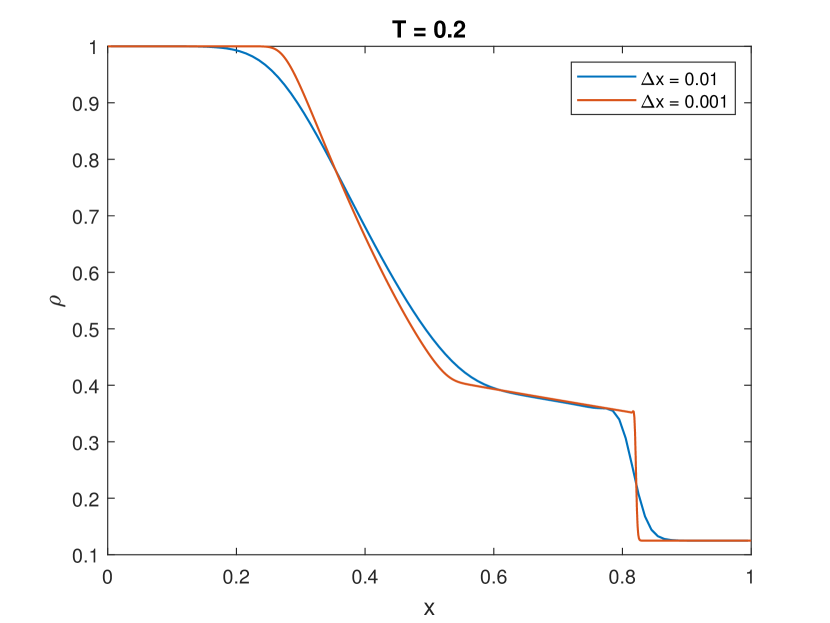
(a)

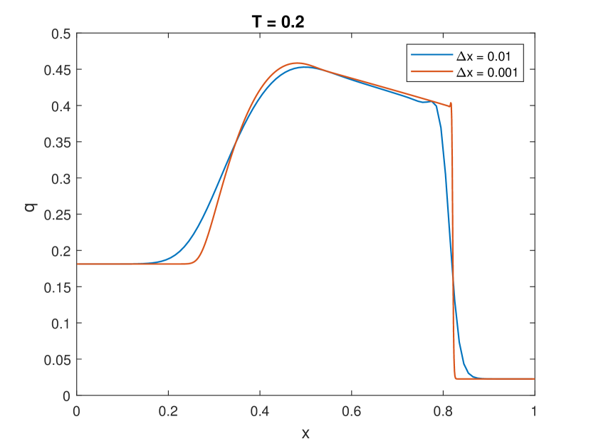
(b)

Figure 1. 1D Sod problem: solution profiles of (A) $\rho$ and (B) $q$ at $T=0.2$ in the non-stiff regime for $\varepsilon=1$.

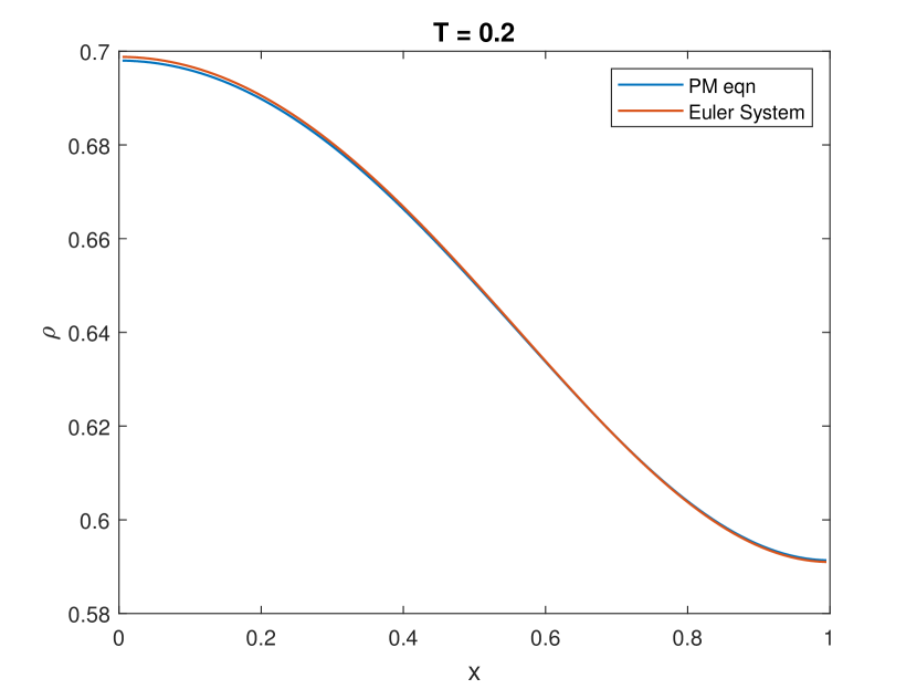
(a)

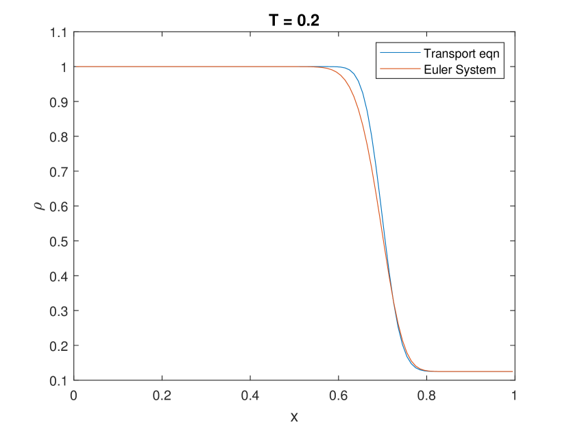
(b)

Figure 2. 1D Sod problem: solution profiles of $\rho$ at $T=0.2$ for $\varepsilon=0.001$ in the (A) parabolic and (B) hyperbolic relaxation regimes.

In the stiff regime, we consider both the hyperbolic and parabolic relaxations. When $\varepsilon=0.001$ by setting $\beta=1$, the numerical solution obtained on a mesh with $100$ cells with $\lambda_{\mathrm{CFL}}=0.45$, is compared with that of a standard first order scheme for the porous medium equation (2.9) to demonstrate the parabolic relaxation. The resulting solution is in perfect agreement with that of the parabolic equation showing the correct asymptotic behaviour of the scheme. Similarly, to show the hyperbolic relaxation for $\beta\in[0,1)$, the scheme is tested for $\beta=0.1$ and $\lambda_{\mathrm{CFL}}=0.45$. The result shows good agreement with a first order upwind scheme applied to the transport equation (2.10).

5.2. Well-balancing Property

To numerically validate the well-balancing property of the scheme, we use initial data in both isothermal and isentropic hydrostatic equilibrium, taken from [49]. We also add a small perturbation to these equilibria to study their evolution via the scheme. Finally, we compute the solution for a large time to show the convergence of the numerical solution to the steady state, and to compare our results with that of a non well-balanced solver. The CFL number $\lambda_{\mathrm{CFL}}$ was taken to be 0.45 in every case.

5.2.1. Isothermal Hydrostatic Solution

We solve the system which is initially in isothermal hydrostatic equilibrium for $\beta=1$ corresponding to the following configuration:

(5.3) $$\rho(0,x)\equiv\rho_{e}(x)=\exp(\phi(x)),\quad u(0,x)\equiv u_{e}(x)=0.$$

The exact solution $(\rho_{e},u_{e})$, cf. (2.13), is interpolated onto the grid, and for different values of $\varepsilon$, the $L^{1}$ errors are calculated for three different gravitational potentials $\phi(x)=x,\frac{x^{2}}{2},\sin(2\pi x)$ for grids with $100$ and $1000$ cells upto a final time $T=2$. It can be seen from Table 1 that the scheme exhibits good precision in approximating the exact hydrostatic solution for the different potentials in both the stiff and non-stiff regimes. Thus we conclude that the scheme maintains the well-balancing property for isothermal hydrostatic solutions.

$\varepsilon=1.0$
$\phi$	$N$	Error in $\rho$	Error in $q$
$x$	100	2.6815E-06	4.1644E-06
	1000	2.7018E-08	4.1655E-08
$x^{2}/2$	100	9.9540E-07	8.6076E-07
	1000	9.7002E-09	8.4871E-09
$\sin(2\pi x)$	100	2.1751E-04	4.3318E-06
	1000	2.0620E-06	6.2102E-08

$\varepsilon=0.1$
$\phi$	$N$	Error in $\rho$	Error in $q$
$x$	100	1.4173E-06	1.1110E-05
	1000	1.4070E-08	1.0878E-07
$x^{2}/2$	100	8.9859E-07	2.1290E-06
	1000	8.7053E-09	2.0610E-08
$\sin(2\pi x)$	100	2.2498E-04	1.4161E-05
	1000	2.1303E-06	1.4130E-08

$\varepsilon=0.01$
$\phi$	$N$	Error in $\rho$	Error in $q$
$x$	100	1.1902E-06	1.3049E-05
	1000	1.1544E-08	1.2975E-07
$x^{2}/2$	100	8.8290E-07	2.4434E-06
	1000	8.5468E-09	2.4053E-08
$\sin(2\pi x)$	100	2.2599E-04	1.6097E-05
	1000	2.1313E-06	1.6134E-08

$\varepsilon=0.001$
$\phi$	$N$	Error in $\rho$	Error in $q$
$x$	100	1.1705E-06	1.3170E-05
	1000	1.1390E-08	1.3172E-07
$x^{2}/2$	100	8.8199E-07	2.4605E-06
	1000	8.5282E-09	2.4367E-08
$\sin(2\pi x)$	100	2.2606E-04	1.6197E-05
	1000	2.1314E-06	1.6336E-08

Table 1. Errors in the density $\rho$ and the momentum $q$ for different potentials and for a range of $\varepsilon$ using different mesh sizes in the isothermal test case.

Next, we want to study the efficacy of the scheme in simulating the evolution of small perturbations added to the initial equilibrium solution. To this end, we compare our solver with a non well-balanced scheme which also makes use of the unified AP time discretisation but without the equilibrium spatial reconstruction. The potential in this case is taken to be $\phi(x)=x$ and the initial density is given by

(5.4) $$\rho_{0}(x)=\exp(\phi(x))+\zeta\exp(-100(x-0.5)^{2}).$$

The computational domain is $[0,1]$ and the boundary conditions are imposed by interpolating the equilibrium solution onto the ghost cells. The results are presented for two different amplitudes of perturbation $\zeta=10^{-3},10^{-5}$. In the non-stiff regime, as expected, the well-balanced scheme resolves the solution well when compared to the non well-balanced scheme, cf. Figure 3. However, we notice from Figure 4 that the non well-balanced scheme also produces results similar to that of the well-balanced scheme in the stiff regime. This behaviour can be explained by the fact that the parabolic porous medium equation (2.9) and the hyperbolic Euler system (2.5)-(2.6) share the same stationary state, and the AP property of the non well-balanced scheme then ensures that it also relaxes to a reasonable approximation of the same steady state as $\varepsilon\to 0$.

(a)

(b)

(c)

Figure 3. Isothermal test: evolution in the density perturbation in the non-stiff regime for $\varepsilon=1$. Comparison of well-balanced scheme with non-well balanced scheme for different values of $\zeta$. (A) $\zeta=10^{-3}$ (B) $\zeta=10^{-5}$. (C) Comparison of well-balanced scheme with initial perturbation for $\zeta=10^{-5}$.

(a)

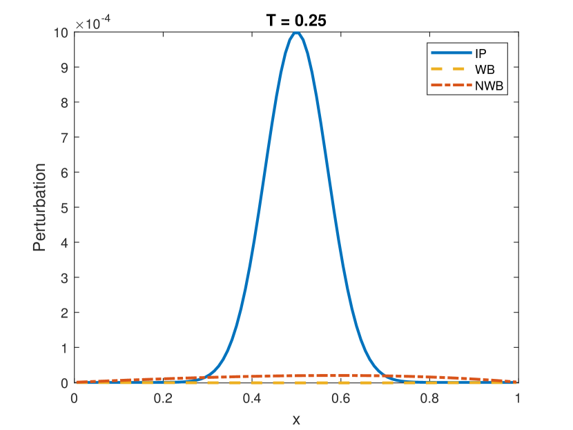
(b)

Figure 4. Isothermal test: evolution in the density perturbation in the stiff regime for $\varepsilon=0.001$ for (a) $\zeta=10^{-3}$ (b) $\zeta=10^{-5}$.

Finally we also study the long time behaviour of the scheme to corroborate its convergence to a steady state by simulating the isothermal hydrostatic solution until a large time $T=100$. We take the initial data (5.4) at equilibrium with a small perturbation with amplitude $\zeta=10^{-3}$. The boundary conditions again the exact solution interpolated onto the grid for the domain $[0,1]$. For $\varepsilon=1$, the momentum converges accurately for the well-balanced scheme but the non well-balanced scheme diverges away from the stationary solution, cf. Figure 5.

(a)

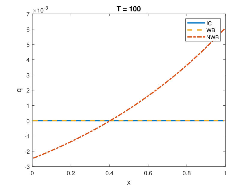
(b)

Figure 5. Isothermal test: long time solution profiles when $\varepsilon=1$ for (A) $\rho$ and (B) $q$.

(a)

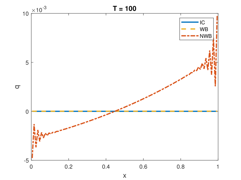
(b)

Figure 6. Isothermal test: long time solution profiles when $\varepsilon=0.1$ for (A) $\rho$ and (B) $q$.

(a)

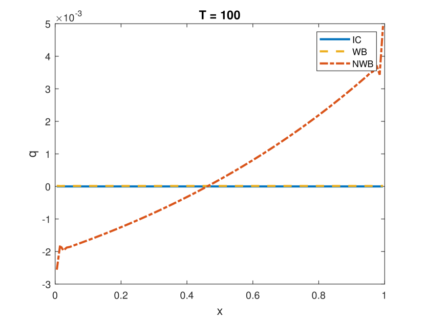
(b)

Figure 7. Isothermal test: long time solution profiles when $\varepsilon=0.01$ for (A) $\rho$ and (B) $q$.

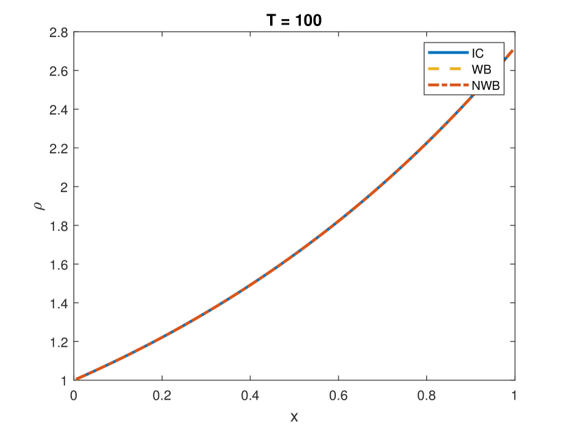
(a)

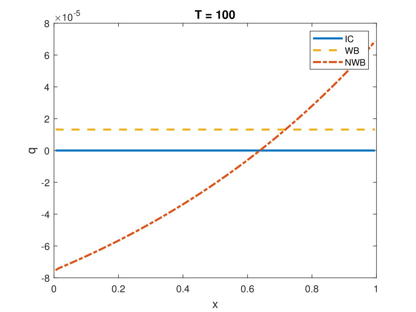
(b)

Figure 8. Isothermal test: long time solution profiles when $\varepsilon=0.001$ for (A) $\rho$ and (B) $q$.

As was noted before, in the asymptotic regime, the non well-balanced AP scheme also exudes the well-balancing property, and hence it can be seen from Figure 8 that the results are comparable with that of the well balanced scheme when $\varepsilon=0.001$. The oscillations that can be seen for intermediate values of the stiffness parameter ($\varepsilon=0.1,0.01$) in Figures 6-7 for the non well-balanced scheme can be attributed to the loss of accuracy for the IMEX scheme in this range of $\varepsilon$; see e.g. [45] for related discussions. From the three above-mentioned test cases, it is evident that the scheme preserves the isothermal hydrostatic solution.

5.2.2. Isentropic Hydrostatic Solution

In this test case, we solve the system which is initially in isentropic hydrostatic equilibrium for $\beta=1$. The initial data reads

(5.5) $$\rho(0,x)\equiv\rho_{e}(x)=\left(1+\frac{\gamma-1}{\gamma}\phi(x)\right)^{\frac{1}{\gamma-1}},\quad u(0,x)\equiv u_{e}(x)=0.$$

The domain is $[0,1]$ and the boundary conditions are interpolation. We also take the specific heat ratio to be $\gamma=1.4$.

First, for a range of $\varepsilon$, we test the $L^{1}$ error of the scheme for different potential functions and for different mesh sizes. The simulations are run for a final time of $T=2.$ Results are presented in Table 2. Similar to the isothermal hydrostatic test case, here too we observe good precision in preserving the steady state solution.

$\varepsilon=1$
$\phi$	N	Error in $\rho$	Error in $q$
$x$	100	3.0399E-07	7.6093E-07
	1000	3.0717E-09	7.4895E-09
$x^{2}/2$	100	1.5297E-07	1.8205E-07
	1000	1.4429E-09	1.7516E-09
sin($2\pi x$)	100	3.5858E-05	1.6335E-06
	1000	3.5668E-07	3.4458E-09

$\varepsilon=0.1$
$\phi$	N	Error in $\rho$	Error in $q$
$x$	100	8.8097E-08	2.2017E-06
	1000	8.9517E-10	2.1593E-08
$x^{2}/2$	100	1.3723E-07	5.0076E-07
	1000	1.2993E-09	4.8594E-09
sin($2\pi x$)	100	3.6382E-05	4.4131E-06
	1000	3.5705E-07	4.4168E-09

$\varepsilon=0.01$
$\phi$	N	Error in $\rho$	Error in $q$
$x$	100	2.2198E-08	2.6719E-06
	1000	2.0347E-10	2.6542E-08
$x^{2}/2$	100	1.3446E-07	5.9381E-07
	1000	1.2895E-09	5.8580E-09
sin($2\pi x$)	100	3.6564E-05	5.1607E-06
	1000	3.5718E-07	5.1886E-09

$\varepsilon=0.001$
$\phi$	N	Error in $\rho$	Error in $q$
$x$	100	1.8445E-08	2.7065E-06
	1000	1.6062E-10	2.7060E-08
$x^{2}/2$	100	1.3427E-07	5.9992E-07
	1000	1.2840E-09	5.9572E-09
sin($2\pi x$)	100	3.6580E-05	5.2108E-06
	1000	3.5719E-07	5.2778E-09

Table 2. Errors in the density $\rho$ and the momentum $q$ for different potentials and for a range of $\varepsilon$ using different mesh sizes in the isentropic test case.

Next, we test the efficacy of the scheme in simulating the evolution of small density perturbations added to the initial data, i.e.

$$\rho(0,x)=\left(1+\frac{\gamma-1}{\gamma}\phi(x)\right)^{\frac{1}{\gamma-1}}+\zeta\text{exp}(-100(x-0.5)^{2}).$$

Simulations are performed upto a final time $T=0.25$ on a mesh of 100 cells with interpolation boundary conditions for $\zeta=10^{-3},10^{-5}$. The results are presented in Figure 9 for the non-stiff regime. Evidently the well-balanced scheme is able to resolve the solution much better than the non well-balanced scheme for both high and low values of $\varepsilon$. In the stiff regime, the non well-balanced scheme’s performance improves due to its AP property as is evident from Figure 10.

Thus in this subsection, we have shown that the scheme performs well in maintaining the steady states of the Euler system for both isothermal and isentropic equations of state with very good accuracy.

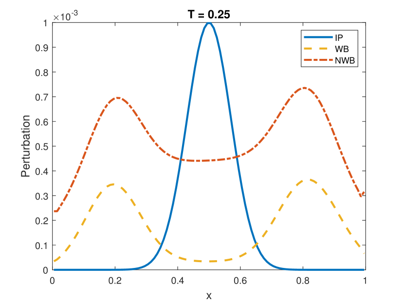
(a)

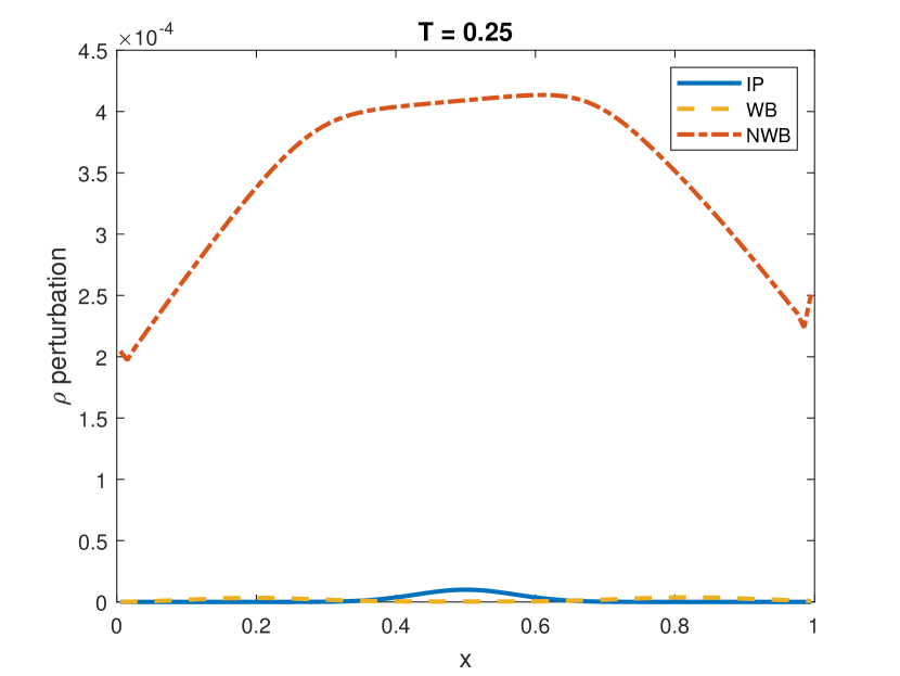
(b)

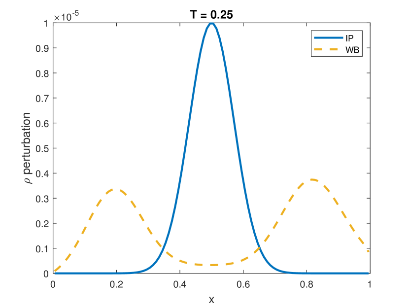
(c)

Figure 9. Isentropic test: evolution in the density perturbation in the non-stiff regime for $\varepsilon=1$. (a) $\zeta=10^{-3}$ (b) $\zeta=10^{-5}$; comparison of well-balanced scheme with non-well balanced (c) $\zeta=10^{-5}$; comparison of well-balanced scheme with initial perturbation.

(a)

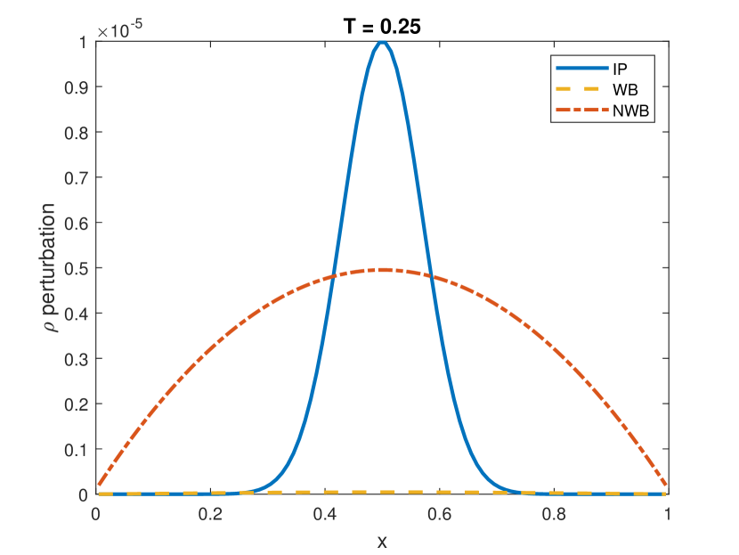
(b)

Figure 10. Isentropic test: evolution in the density perturbation in the stiff regime for $\varepsilon=0.001$ for (a) $\zeta=10^{-3}$ (b) $\zeta=10^{-5}$.

5.3. Sensitivity to Mesh Size

In this test, our aim is to study the dependence of the accuracy of the scheme on mesh sizes in the asymptotic regime ($\varepsilon=0.001$) by comparing it with a non AP scheme. For this purpose, the initial data as given in [15] which is a centered arch function and it reads

(5.6) $$(\rho,u)=\begin{cases}(1,0),&\text{if}\ -0.2<x<0.2,\\ (2,0),&\text{otherwise},\end{cases}$$

in the domain $[-0.5,0.5]$ with periodic boundary conditions and $\lambda_{\mathrm{CFL}}=0.45$. The test is carried out for both hyperbolic and parabolic relaxations. Figure 11(a) shows that the AP scheme’s performance does not show any dependence on the mesh sizes, giving almost identical results for under-resolved ($\Delta x=0.01$), resolved ($\Delta x=0.001$), and over-resolved ($\Delta x=0.0001$) meshes in the parabolic regime. However, the non AP scheme blows up for the under-resolved mesh (Figure 11(b)), but it shows results similar to the AP scheme for the resolved and over-resolved meshes as can be seen from Figure 11(c). Similar conclusions can again be drawn in the case of hyperbolic relaxation. Results are presented in Figure 12. Even though a blowup is not observed for the non AP scheme, oscillations can be seen at the discontinuities on the under-resolved mesh.

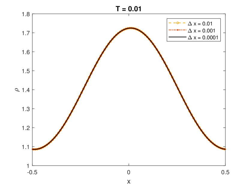
(a)

(b)

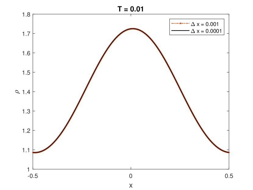
(c)

Figure 11. Mesh sensitivity test: solution profile of $\rho$ for different mesh sizes for $\varepsilon=0.001$ (A) AP scheme (B) non AP scheme, $\Delta x=0.01$ (C) non AP scheme, $\Delta x=0.001,0.0001$.

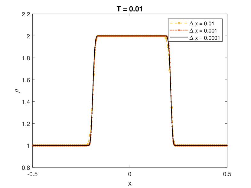
(a)

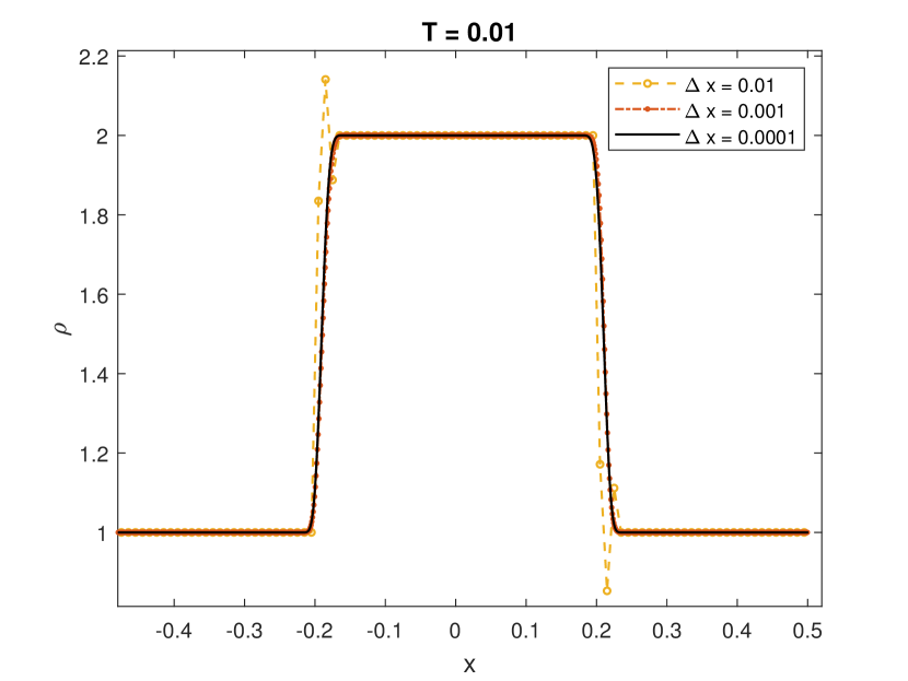
(b)

Figure 12. Mesh sensitivity test: solution profile of $\rho$ for different mesh sizes for different mesh sizes when $\varepsilon=0.001$ (A) AP scheme (B) non AP scheme.

6. Concluding Remarks

We have designed and analysed a unified AP scheme which captures both the hyperbolic and parabolic limits of the Euler system with gravity and friction. The time semi-discrete and semi-implicit scheme is based on the ideas presented in [7]. A reformulation of the semi-implicit scheme admits a fully-explicit formulation which is stable under a parabolic CFL condition. Though for the hyperbolic relaxation the time steps are dependent on $\varepsilon$, the CFL restriction does not degrade; rather it becomes less and less severe as $\varepsilon\to 0$. A fully-discrete scheme is obtained using a finite volume treatment which makes use of an equilibrium reconstruction of the interface values, source term upwinding and a gingerly choice of central discretisation for the mass update. Both the semi-discrete and space-time fully-discrete scheme are shown to be AP for both the hyperbolic and parabolic limit equations. Furthermore, the fully-discrete scheme is shown to well-balanced for hydrostatic steady states. The numerical case studies presented clearly demonstrate the AP and well-balancing properties of the developed scheme. They also showcase the superiority of the designed scheme over its non well-balanced and non AP counterparts. In conclusion, the aim of developing a unified AP and well-balanced scheme is achieved and is justified through the material presented in the paper.

References

- [1] G. Albi, G. Dimarco, and L. Pareschi. Implicit-explicit multistep methods for hyperbolic systems with multiscale relaxation. SIAM J. Sci. Comput., 42(4):A2402–A2435, 2020.
- [2] D. Aregba-Driollet and R. Natalini. Convergence of relaxation schemes for conservation laws. Appl. Anal., 61(1-2):163–193, 1996.
- [3] K. R. Arun and S. Samantaray. Asymptotic preserving low Mach number accurate IMEX finite volume schemes for the isentropic Euler equations. J. Sci. Comput., 82(2):Art. 35, 32, 2020.
- [4] E. Audusse, F. Bouchut, M.-O. Bristeau, R. Klein, and B. Perthame. A fast and stable well-balanced scheme with hydrostatic reconstruction for shallow water flows. SIAM J. Sci. Comput., 25(6):2050–2065, 2004.
- [5] G. Bispen, K. R. Arun, M. Lukáčová-Medvid’ová, and S. Noelle. IMEX large time step finite volume methods for low Froude number shallow water flows. Commun. Comput. Phys., 16(2):307–347, 2014.
- [6] G. Bispen, M. Lukáčová-Medviďová, and L. Yelash. Asymptotic preserving IMEX finite volume schemes for low Mach number Euler equations with gravitation. J. Comput. Phys., 335:222–248, 2017.
- [7] S. Boscarino, L. Pareschi, and G. Russo. A unified IMEX Runge-Kutta approach for hyperbolic systems with multiscale relaxation. SIAM J. Numer. Anal., 55(4):2085–2109, 2017.
- [8] S. Boscarino and G. Russo. Flux-explicit IMEX Runge-Kutta schemes for hyperbolic to parabolic relaxation problems. SIAM J. Numer. Anal., 51(1):163–190, 2013.
- [9] F. Bouchut. Construction of BGK models with a family of kinetic entropies for a given system of conservation laws. J. Statist. Phys., 95(1-2):113–170, 1999.
- [10] F. Bouchut. Nonlinear stability of finite volume methods for hyperbolic conservation laws and well-balanced schemes for sources. Frontiers in Mathematics. Birkhäuser Verlag, Basel, 2004.
- [11] F. Bouchut, E. Franck, and L. Navoret. A low cost semi-implicit low-Mach relaxation scheme for the full Euler equations. J. Sci. Comput., 83(1):Paper No. 24, 47, 2020.
- [12] R. E. Caflisch, S. Jin, and G. Russo. Uniformly accurate schemes for hyperbolic systems with relaxation. SIAM J. Numer. Anal., 34(1):246–281, 1997.
- [13] C. Cercignani. The Boltzmann equation and its applications, volume 67 of Applied Mathematical Sciences. Springer-Verlag, New York, 1988.
- [14] C. Cercignani, R. Illner, and M. Pulvirenti. The mathematical theory of dilute gases, volume 106 of Applied Mathematical Sciences. Springer-Verlag, New York, 1994.
- [15] C. Chalons, F. Coquel, E. Godlewski, P.-A. Raviart, and N. Seguin. Godunov-type schemes for hyperbolic systems with parameter-dependent source. The case of Euler system with friction. Math. Models Methods Appl. Sci., 20(11):2109–2166, 2010.
- [16] S. Chapman and T. G. Cowling. The Mathematical Theory of Non-uniform Gases. Cambridge University Press, Cambridge, 1939.
- [17] G. Q. Chen, C. D. Levermore, and T.-P. Liu. Hyperbolic conservation laws with stiff relaxation terms and entropy. Comm. Pure Appl. Math., 47(6):787–830, 1994.
- [18] A. Chinnayya, A.-Y. LeRoux, and N. Seguin. A well-balanced numerical scheme for the approximation of the shallow-water equations with topography: the resonance phenomenon. Int. J. Finite Vol., 1(1):33, 2004.
- [19] P. Degond and M. Tang. All speed scheme for the low Mach number limit of the isentropic Euler equations. Commun. Comput. Phys., 10(1):1–31, 2011.
- [20] G. Dimarco, R. Loubère, and M.-H. Vignal. Study of a new asymptotic preserving scheme for the Euler system in the low Mach number limit. SIAM J. Sci. Comput., 39(5):A2099–A2128, 2017.
- [21] G. Dimarco and L. Pareschi. Exponential Runge-Kutta methods for stiff kinetic equations. SIAM J. Numer. Anal., 49(5):2057–2077, 2011.
- [22] U. S. Fjordholm, S. Mishra, and E. Tadmor. Well-balanced and energy stable schemes for the shallow water equations with discontinuous topography. J. Comput. Phys., 230(14):5587–5609, 2011.
- [23] J. M. Gallardo, C. Parés, and M. Castro. On a well-balanced high-order finite volume scheme for shallow water equations with topography and dry areas. J. Comput. Phys., 227(1):574–601, 2007.
- [24] L. Gosse. A well-balanced flux-vector splitting scheme designed for hyperbolic systems of conservation laws with source terms. Comput. Math. Appl., 39(9-10):135–159, 2000.
- [25] J. M. Greenberg and A. Y. Leroux. A well-balanced scheme for the numerical processing of source terms in hyperbolic equations. SIAM J. Numer. Anal., 33(1):1–16, 1996.
- [26] S. Jin. Runge-Kutta methods for hyperbolic conservation laws with stiff relaxation terms. J. Comput. Phys., 122(1):51–67, 1995.
- [27] S. Jin. Efficient asymptotic-preserving (AP) schemes for some multiscale kinetic equations. SIAM J. Sci. Comput., 21(2):441–454, 1999.
- [28] S. Jin. Asymptotic preserving (AP) schemes for multiscale kinetic and hyperbolic equations: a review. Riv. Math. Univ. Parma (N.S.), 3(2):177–216, 2012.
- [29] S. Jin and C. D. Levermore. Numerical schemes for hyperbolic conservation laws with stiff relaxation terms. J. Comput. Phys., 126(2):449–467, 1996.
- [30] S. Jin, L. Pareschi, and G. Toscani. Diffusive relaxation schemes for multiscale discrete-velocity kinetic equations. SIAM J. Numer. Anal., 35(6):2405–2439, 1998.
- [31] S. Jin, L. Pareschi, and G. Toscani. Uniformly accurate diffusive relaxation schemes for multiscale transport equations. SIAM J. Numer. Anal., 38(3):913–936, 2000.
- [32] S. Jin and Z. P. Xin. The relaxation schemes for systems of conservation laws in arbitrary space dimensions. Comm. Pure Appl. Math., 48(3):235–276, 1995.
- [33] S. Klainerman and A. Majda. Singular limits of quasilinear hyperbolic systems with large parameters and the incompressible limit of compressible fluids. Comm. Pure Appl. Math., 34(4):481–524, 1981.
- [34] A. Klar. An asymptotic-induced scheme for nonstationary transport equations in the diffusive limit. SIAM J. Numer. Anal., 35(3):1073–1094, 1998.
- [35] A. Kurganov and G. Petrova. A second-order well-balanced positivity preserving central-upwind scheme for the Saint-Venant system. Commun. Math. Sci., 5(1):133–160, 2007.
- [36] M. Lemou and L. Mieussens. A new asymptotic preserving scheme based on micro-macro formulation for linear kinetic equations in the diffusion limit. SIAM J. Sci. Comput., 31(1):334–368, 2008.
- [37] T.-P. Liu. Hyperbolic conservation laws with relaxation. Comm. Math. Phys., 108(1):153–175, 1987.
- [38] R. Natalini. Convergence to equilibrium for the relaxation approximations of conservation laws. Comm. Pure Appl. Math., 49(8):795–823, 1996.
- [39] R. Natalini. Recent results on hyperbolic relaxation problems. In Analysis of systems of conservation laws (Aachen, 1997), volume 99 of Chapman & Hall/CRC Monogr. Surv. Pure Appl. Math., pages 128–198. Chapman & Hall/CRC, Boca Raton, FL, 1999.
- [40] R. Natalini, M. Ribot, and M. Twarogowska. A well-balanced numerical scheme for a one dimensional quasilinear hyperbolic model of chemotaxis. Commun. Math. Sci., 12(1):13–39, 2014.
- [41] R. Natalini, M. Ribot, and M. Twarogowska. A numerical comparison between degenerate parabolic and quasilinear hyperbolic models of cell movements under chemotaxis. J. Sci. Comput., 63(3):654–677, 2015.
- [42] S. Noelle, G. Bispen, K. R. Arun, M. Lukáčová-Medviďová, and C.-D. Munz. A weakly asymptotic preserving low Mach number scheme for the Euler equations of gas dynamics. SIAM J. Sci. Comput., 36(6):B989–B1024, 2014.
- [43] S. Noelle, N. Pankratz, G. Puppo, and J. R. Natvig. Well-balanced finite volume schemes of arbitrary order of accuracy for shallow water flows. J. Comput. Phys., 213(2):474–499, 2006.
- [44] S. Noelle, Y. Xing, and C.-W. Shu. High-order well-balanced finite volume WENO schemes for shallow water equation with moving water. J. Comput. Phys., 226(1):29–58, 2007.
- [45] L. Pareschi and G. Russo. Implicit-explicit Runge-Kutta schemes for stiff systems of differential equations. In Recent trends in numerical analysis, volume 3 of Adv. Theory Comput. Math., pages 269–288. Nova Sci. Publ., Huntington, NY, 2001.
- [46] L. Pareschi and G. Russo. Implicit-Explicit Runge-Kutta schemes and applications to hyperbolic systems with relaxation. J. Sci. Comput., 25(1-2):129–155, 2005.
- [47] B. Perthame and C. Simeoni. Convergence of the upwind interface source method for hyperbolic conservation laws. In Hyperbolic problems: theory, numerics, applications, pages 61–78. Springer, Berlin, 2003.
- [48] A. Thomann, G. Puppo, and C. Klingenberg. An all speed second order well-balanced IMEX relaxation scheme for the Euler equations with gravity. J. Comput. Phys., 420:109723, 25, 2020.
- [49] D. Varma and P. Chandrashekar. A second-order, discretely well-balanced finite volume scheme for Euler equations with gravity. Comput. & Fluids, 181:292–313, 2019.
- [50] G. B. Whitham. Linear and nonlinear waves. Wiley-Interscience [John Wiley & Sons], New York-London-Sydney, 1974. Pure and Applied Mathematics.
- [51] Y. Xing and C.-W. Shu. High order finite difference WENO schemes with the exact conservation property for the shallow water equations. J. Comput. Phys., 208(1):206–227, 2005.
- [52] Y. Xing and C.-W. Shu. High order well-balanced finite volume WENO schemes and discontinuous Galerkin methods for a class of hyperbolic systems with source terms. J. Comput. Phys., 214(2):567–598, 2006.
- [53] K. Xu. A well-balanced gas-kinetic scheme for the shallow-water equations with source terms. J. Comput. Phys., 178(2):533–562, 2002.