Flat-band ferromagnetism and spin waves in the Haldane-Hubbard model

Abstract

We study the flat-band ferromagnetic phase of the Haldane-Hubbard model on a honeycomb lattice within a bosonization scheme for flat-band Chern insulators, focusing on the calculation of the spin-wave excitation spectrum. We consider the Haldane-Hubbard model with the noninteracting lower bands in a nearly-flat band limit, previously determined for the spinless model, and at $1/4$-filling of its corresponding noninteracting limit. Within the bosonization scheme, the Haldane-Hubbard model is mapped into an effective interacting boson model, whose quadratic term allows us to determine the spin-wave spectrum at the harmonic approximation. We show that the excitation spectrum has two branches with a Goldstone mode and Dirac points at center and at the $K$ and $K^{\prime}$ points of the first Brillouin zone, respectively. We also consider the effects on the spin-wave spectrum due to an energy offset in the on-site Hubbard repulsion energies and due to the presence of an staggered on-site energy term, both quantities associated with the two triangular sublattices. In both cases, we find that an energy gap opens at the $K$ and $K^{\prime}$ points. Moreover, we also find some evidences for an instability of the flat-band ferromagnetic phase in the presence of the staggered on-site energy term. We provide some additional results for the square lattice topological Hubbard model previous studied within the bosonization formalism and comment on the differences between the bosonization scheme implementation for the correlated Chern insulators on both square and honeycomb lattices.

I Introduction

The tight-binding model on a honeycomb lattice with broken time-reversal symmetry proposed by Haldane haldane1988model is an interesting example of a Chern band insulator kane13 ; rpp-rachel18 . At half-filling, it can exhibit a quantized Hall conductance in the absence of an external magnetic field. This so-called anomalous quantum Hall effect qi11 is indeed related to the fact that the electronic band structure of Haldane’s model is topologically nontrivial, i.e., the corresponding Chern numbers of each band are finite kane13 ; rpp-rachel18 . Interestingly, the model was experimentally implemented in a system with ultracold fermions in an optical honeycomb lattice jotzu14 (see also the reviews zoller16 ; rmp-cooper19 ).

A lot of effort has also been devoted to the study of the interplay between the topological properties of electronic band structures and the electron-electron interaction rpp-rachel18 ; assaad13 . A particular correlated Chern insulator that has been receiving some attention in recents years is a natural extension of Haldane’s model haldane1988model , the so-called Haldane-Hubbard model he2011chiral ; he2011topological ; maciejko2013topological ; hickey15 ; hickey2016haldane ; zheng15 ; vanhala16 ; wu2016quantum ; arun16 ; troyer16 . Here the electronic spin is explicitly taken into account, time-reversal symmetry is broken, and correlation effects are described via an on-site Hubbard repulsion term [see Eq. (1) below]. At half-filling, the phase diagram of the Haldane-Hubbard model has been determined via different mean-field approaches he2011chiral ; he2011topological ; hickey15 ; zheng15 ; arun16 and numerical methods hickey2016haldane ; vanhala16 ; wu2016quantum ; troyer16 . It was shown that the model supports a Chern insulator phase for weak interactions and a trivial Néel magnetic ordered phase for strong ones. Moreover, there are evidences for a first-order transition between these two phases troyer16 , but also for the presence of a distinct phase in the intermediate coupling region he2011chiral ; he2011topological ; wu2016quantum . Differently from the time-reversal symmetric Kane-Mele Hubbard model rpp-rachel18 , the breaking of time-reversal symmetry in the Haldane-Hubbard model yields the so-called fermion sign problem, limiting the use of quantum Monte Carlo simulations wu2016quantum ; troyer16 .

Away from half-filling, the study of correlation effects in Chern band insulators have also considered the possibility of realizing fractional quantum Hall phases in lattice models. Indeed, the interest in fractional Chern insulators sondhi13 ; liu13 ; neupert15 was motivated by the studies neupert2011fractional ; sun2011nearly ; tang2011high , which showed that a series of tight-binding models with only short-range hoppings can display nearly-flat and topologically nontrivial electronic bands once the model parameters are properly chosen. Due to the similarity between flat bands with nonzero Chern numbers and Landau levels realized in a two-dimensional electron gas, it was proposed that these lattice models could display a fractional quantum Hall effect for partially filled bands if electron-electron interaction is taking into account neupert2011fractional ; sun2011nearly ; tang2011high . Indeed, numerical evidences for the stability of fractional Chern insulator phases were later reported sheng11 ; regnault11 . We should mention that, recently, the infinite density matrix renormalization group (iDMRG) technique was employ to study the stability of fractional quantum Hall states in correlated Hofstadter-like models andrews20 ; andrews21 .

Correlation effects in a spinfull topological Hubbard model on a square lattice with nearly-flat noninteracting bands but at a commensurate filling were also discussed neupert2012topological ; doretto2015flat ; su2019ferromagnetism . Here the noninteracting limit of the topological Hubbard model is given by the $\pi$-flux model, whose parameters can be adjusted such that the band structure is given by two lower and two higher (doubly degenerated) nearly-flat bands separated by an energy gap neupert2011fractional . At $1/4$-filling (half-filling of the lower band), it was shown neupert2012topological ; doretto2015flat ; su2019ferromagnetism that such topological Hubbard model can realize a flat-band ferromagnetic phase flat-fm . In particular, one of us calculated the spin-wave excitation spectrum of the flat-band ferromagnetic phase within a bosonization formalism doretto2015flat . For the corresponding correlated Chern insulator, it was shown that the spin-wave spectrum has one gapped excitation branch and one gapless one, with the Goldstone mode at the centre of the first Brillouin zone. These analytical results qualitatively agrees with the numerical ones determined via exact diagonalization su2019ferromagnetism .

Figure 1: (a) Schematic representation of the Haldane-Hubbard model (1) on the honeycomb lattice, indicating the nearest-neighbor $t_{1}$ and next-nearest-neighbor $t_{2}e^{\pm i\phi}$ hoppings and the on-site Hubbard repulsion energy $U_{a}$. Blue and red circles indicate the sites of the (triangular) sublattices $A$ and $B$, respectively. $\mbox{\boldmath$\delta$}_{i}$ and $\mbox{\boldmath$\tau$}_{i}$ are the nearest-neighbor (4) and next-nearest-neighbor (5) vectors, respectively. (b) The first Brillouin zone and it’s highly symmetrical points: $\mathbf{K}=(4\pi/3\sqrt{3},0)$, $\mathbf{K^{\prime}}=(2\pi/3\sqrt{3},2\pi/3)$, $\mathbf{M}_{1}=(\pi/\sqrt{3},\pi/3)$, and $\mathbf{M}_{2}=(0,2\pi/3)$. The nearest-neighbor distance of the honeycomb lattice $a=1$.

In the present paper, we study the flat-band ferromagnetic phase of a correlated Chern insulator on a honeycomb lattice described by the Haldane-Hubbard model. We consider configurations close to the nearly-flat band limit of the lower (noninteracting) bands that was previously determined for the (spinless) Haldane model neupert2011fractional . We describe the flat-band ferromagnetic phase of the Haldane-Hubbard model within the bosonization formalism for flat-band correlated Chern insulators proposed in Ref. doretto2015flat . Such a bosonization scheme is based on the method proposed to study the quantum Hall ferromagnetic phase of a two-dimensional electron gas at filling factor $\nu=1$ doretto2005lowest . It was later employed to described the quantum Hall ferromagnetic phases realized in graphene at filling factors $\nu=0$ and $\nu=\pm 1$ doretto2007quantum . We show that the bosonization scheme allow us to map the Haldane-Hubbard model at the nearly-flat band limit of its lower band to an effective interacting boson model. Our main finding is the flat-band ferromagnetic phase spin-wave spectrum, which corresponds to the dispersion relation of the bosons determined from the effective boson model within a harmonic approximation. We find that the spin-wave excitation spectrum has one gapped and one gapless excitation branches, with a Goldstone mode at the center of the first Brillouin zone and Dirac points at the $K$ and $K^{\prime}$ points [see Fig. 6(a), below]. Introducing an energy offset in the on-site Hubbard repulsion energies associated with the (triangular) sublattices $A$ and $B$, one finds that an energy gap opens in the spin-wave excitation spectrum at the $K$ and $K^{\prime}$ points. The effects on the spin-wave spectrum due to the presence of a staggered on-site energy term related to the sublattices $A$ and $B$ is also discussed.

Our paper is organized as follows. In Sec. II, we introduce the Haldane-Hubbard model on a honeycomb lattice and discuss in details the band structure of the noninteracting term close to the nearly flat-band limit determined in Ref. neupert2011fractional . In Sec. III, we briefly review the bosonization scheme for flat-band Chern insulators doretto2015flat . Sec. IV is devoted to the description of the flat-band ferromagnetic phase of the Haldane-Hubbard model: we quote the expression of the effective interacting boson model derived within the bosonization scheme and determine the spin-wave excitation spectra in the nearly flat-band limit and slightly away from this limit; the effects of an energy offset in the on-site Hubbard repulsion term and of a staggered on-site energy term are also discussed. In Sec. V, we discuss our results and provide a brief summary of our main findings. Details of the bosonization formalism are presented in Appendices A and B while additional results derived within the bosonization scheme for the topological Hubbard model on a square lattice previously studied in Ref. doretto2015flat are reported in Appendix C.

II Haldane-Hubbard model

Let us consider $N_{e}$ spin-$1/2$ electrons on a honeycomb lattice described by the Haldane-Hubbard model, whose Hamiltonian is given by he2011chiral ; he2011topological ; maciejko2013topological ; hickey15 ; hickey2016haldane ; zheng15 ; vanhala16 ; wu2016quantum ; arun16 ; troyer16 .

$$H=H_{0}+H_{U},$$ (1)

where

$$H_{0} =t_{1}\sum_{i\in A,\delta,\sigma}\left(c_{iA\sigma}^{\dagger}c_{i+\delta B\sigma}+{\rm H.c.}\right)$$

$$+t_{2}\sum_{i\in A,\tau,\sigma}\left(e^{-i\phi}c_{iA\sigma}^{\dagger}c_{i+\tau A\sigma}+{\rm H.c.}\right)$$

$$+t_{2}\sum_{i\in B,\tau,\sigma}\left(e^{+i\phi}c_{iB\sigma}^{\dagger}c_{i+\tau B\sigma}+{\rm H.c.}\right)$$ (2)

and

$$H_{U}=\sum_{i}\sum_{a=A,B}U_{a}\hat{\rho}_{ia\uparrow}\hat{\rho}_{ia\downarrow}.$$ (3)

Here the operator $c_{ia\sigma}^{\dagger}$ ($c_{ia\sigma}$) creates (destroys) an electron with spin $\sigma=\uparrow,\downarrow$ on site $i$ of the (triangular) sublattice $a=A$, $B$ of the honeycomb lattice. $t_{1}\geq 0$ and $t_{2}e^{\pm i\phi}$ with $t_{2}\geq 0$ are, respectively, the nearest-neighbor and next-nearest-neighbor hoppings. One notices that the electron acquires a $+\phi$ ($-\phi$) phase as it moves in the same (opposite) direction of the arrows within the same sublattice [see dashed lines in Fig. 1(a)]. Indeed, the complex next-nearest-neighbor hopping $t_{2}e^{\pm i\phi}$ results in a fictitious flux pattern with zero net flux per unit cell [see, e.g, Fig. 1(a) from Ref. neupert2011fractional for details]. The index $\delta$ corresponds to the nearest-neighbor vectors [Fig. 1(a)]

$$\mbox{\boldmath$\delta$}_{1} =-a\hat{y},$$

$$\mbox{\boldmath$\delta$}_{2} =\frac{a}{2}\left(\sqrt{3}\hat{x}+\hat{y}\right),\quad\quad\mbox{\boldmath$\delta$}_{3}=-\frac{a}{2}\left(\sqrt{3}\hat{x}-\hat{y}\right),$$ (4)

while $\tau$ indicates the next-nearest-neighbor vectors

$$\mbox{\boldmath$\tau$}_{1} =\mbox{\boldmath$\delta$}_{2}-\mbox{\boldmath$\delta$}_{3}=a\sqrt{3}\hat{x},$$

$$\mbox{\boldmath$\tau$}_{2} =\mbox{\boldmath$\delta$}_{3}-\mbox{\boldmath$\delta$}_{1}=-\frac{a}{2}\left(\sqrt{3}\hat{x}-3\hat{y}\right),$$

$$\mbox{\boldmath$\tau$}_{3} =\mbox{\boldmath$\delta$}_{1}-\mbox{\boldmath$\delta$}_{2}=-\frac{a}{2}\left(\sqrt{3}\hat{x}+3\hat{y}\right).$$ (5)

In the following, we set the nearest-neigbhor distance to unit, i.e., $a=1$. Finally, the $H_{U}$ term [Eq. (3)] is the one-site Hubbard repulsion term, which represents an energy cost paid by double occupation of site $i$, and

$$\hat{\rho}_{ia\sigma}=c_{ia\sigma}^{\dagger}c_{ia\sigma}$$ (6)

is the density operator associated with electrons with spin $\sigma$ at site $i$ of sublattice $a$. We consider that the one-site repulsion energy $U_{a}>0$ can depend on the sublattice $a$.

II.1 Tight-binding term with nearly-flat topological bands

In this section, we discuss in details the noninteracting term $H_{0}$ [Eq. (2)] of the Hamiltonian (1) and show that it can display an almost flat (lower) electronic band that is topologically nontrivial.

             

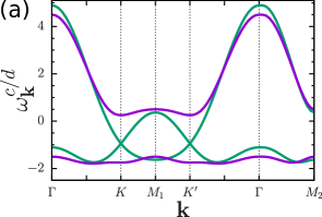
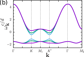
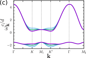
Figure 2: Band structure (19) of the noninteracting hopping term (2) (in units of the nearest-neighbor hopping amplitude $t_{1}$) along paths in the first Brillouin zone [Fig. 1(b)] for different values of the next-nearest-neighbor hopping amplitude $t_{2}$ and phase $\phi$: (a) $t_{2}=0.3155\,t_{1}$, $\phi=0$ (green) and $t_{2}=0.3155\,t_{1}$, $\phi=0.656$ (magenta); (b) $\phi=0.4$ (blue), $\phi=0.5$ (green), and $\phi=0.656$ (magneta), with $t_{2}$ given by the relation $\cos(\phi)=t_{1}/(4t_{2})$; and (c) $\phi=0.656$ (magneta) $\phi=0.75$ (green), and $\phi=0.85$ (blue), with $t_{2}$ given by the relation $\cos(\phi)=t_{1}/(4t_{2})$.

The first step to diagonalize the free-electron Hamiltonian (2) is to perform a Fourier transform,

$$c_{ia\sigma}^{\dagger}=\frac{1}{\sqrt{N_{a}}}\sum_{{\bf k}\in{\rm BZ}}e^{-i\mathbf{k}\cdot\mathbf{R}_{i}}c_{\mathbf{k}\,a\,\sigma}^{\dagger},$$ (7)

where the momentum sum runs over the first Brillouin zone (BZ) [Fig. 1(b)] associated with the underline triangular Bravais lattice and $N_{a}=N$ is the number of sites of the sublattice $a$. It is then easy to show that the noninteracting Hamiltonian (2) can be written in a matrix form,

$$H_{0}=\sum_{\mathbf{k}}\Psi_{\mathbf{k}}^{\dagger}H_{\bf k}\Psi_{\mathbf{k}},$$ (8)

where the $4\times 4$ $H_{\bf k}$ matrix reads

$$H_{\bf k}=\left(\begin{array}[]{cc}h^{\uparrow}_{\mathbf{k}}&0\\ 0&h^{\downarrow}_{\mathbf{k}}\end{array}\right)$$ (9)

and the four-component spinor $\Psi_{\mathbf{k}}$ is given by

$$\Psi_{\mathbf{k}}=\left(c_{\mathbf{k}A\uparrow}\;\;c_{\mathbf{k}B\uparrow}\;\;c_{\mathbf{k}A\downarrow}\;\;c_{\mathbf{k}B\downarrow}\right)^{T}.$$ (10)

The $2\times 2$ matrices $h^{\sigma}_{\bf k}$ associated with each spin sector are such that $h^{\uparrow}_{\bf k}=h^{\downarrow}_{\bf k}=h_{\bf k}$, with the $h_{\bf k}$ matrix given by

$$h_{\bf k} =\left(\begin{array}[]{cc}2t_{2}\sum_{\tau}\cos(\mathbf{k}\cdot\mbox{\boldmath$\tau$}+\phi)&t_{1}\sum_{\delta}e^{i\mathbf{k}\cdot\mbox{\boldmath$\delta$}}\\ t_{1}\sum_{\delta}e^{-i\mathbf{k}\cdot\mbox{\boldmath$\delta$}}&2t_{2}\sum_{\tau}\cos(\mathbf{k}\cdot\mbox{\boldmath$\tau$}-\phi)\end{array}\right).$$ (13)

It is possible to write the $h_{\bf k}$ matrix in terms of the identity matrix $\tau_{0}$ and the vector $\hat{\tau}=(\tau_{1}$, $\tau_{2}$ ,$\tau_{3})$, whose components are Pauli matrices,

$$h_{\bf k}=B_{0,\mathbf{k}}\tau_{0}+\mathbf{B}_{\mathbf{k}}\cdot\hat{\tau},$$ (14)

where the $B_{0,\mathbf{k}}$ function and the components of the vector $\mathbf{B}_{\mathbf{k}}=(B_{1,\mathbf{k}},B_{2,\mathbf{k}},B_{3,\mathbf{k}})$ are given by

$$B_{0,\mathbf{k}} =2t_{2}\cos(\phi)\sum_{\mathbf{\tau}}\cos(\mathbf{k}\cdot\mbox{\boldmath$\tau$}),$$

$$B_{1,\mathbf{k}} =t_{1}\sum_{\mathbf{\delta}}\cos(\mathbf{k}\cdot\mbox{\boldmath$\delta$}),$$

$$B_{2,\mathbf{k}} =t_{1}\sum_{\mathbf{\delta}}\sin(\mathbf{k}\cdot\mbox{\boldmath$\delta$}),$$

$$B_{3,\mathbf{k}} =-2t_{2}\sin(\phi)\sum_{\mathbf{\tau}}\sin(\mathbf{k}\cdot\mbox{\boldmath$\tau$}),$$ (15)

with the indices $\delta$ and $\tau$ corresponding to the nearest-neighbor (4) and next-nearest-neighbor (5) vectors, respectively. The fact that the matrices $h^{\sigma}_{\bf k}$ related to each spin sector $h^{\uparrow}_{\bf k}=h^{\downarrow}_{\bf k}=h_{\bf k}$ indicates that the noninteracting model (2) breaks time-reversal symmetry (see, e.g, Appendix A from Ref. doretto2015flat for details).

The Hamiltonian (8) can be diagonalized via the canonical transformation

$$d_{\mathbf{k}\sigma}=u_{\mathbf{k}}c_{\mathbf{k}A\sigma}+v_{\mathbf{k}}c_{\mathbf{k}B\sigma},$$

$$c_{\mathbf{k}\sigma}=v_{\mathbf{k}}^{*}c_{\mathbf{k}A\sigma}-u_{\mathbf{k}}^{*}c_{\mathbf{k}B\sigma},$$ (16)

where the coefficients $u_{\bf k}$ and $v_{\bf k}$ are given by

$$|u_{\mathbf{k}}|^{2} =\frac{1}{2}\left(1+\hat{B}_{3,\mathbf{k}}\right),\quad|v_{\mathbf{k}}|^{2}=\frac{1}{2}\left(1-\hat{B}_{3,\mathbf{k}}\right),$$

$$u_{\mathbf{k}}v_{\mathbf{k}}^{*} =\frac{1}{2}\left(\hat{B}_{1,\mathbf{k}}+i\hat{B}_{2,\mathbf{k}}\right),$$ (17)

with the hatted $B_{i}$ standing for the $i$-component of the normalized vector $\hat{\mathbf{B}}_{\bf k}=\mathbf{B}_{\bf k}/|\mathbf{B}_{\bf k}|$. After the diagonalization, the Hamiltonian (8) then reads

$$H_{0}=\sum_{\mathbf{k}\sigma}\omega_{\mathbf{k}}^{c}c_{\mathbf{k}\sigma}^{\dagger}c_{\mathbf{k}\sigma}+\omega_{\mathbf{k}}^{d}d_{\mathbf{k}\sigma}^{\dagger}d_{\mathbf{k}\sigma},$$ (18)

with the dispersions of the lower band $c$ ($-$ sign) and the upper one $d$ ($+$ sign) given by

$$\omega^{d/c}_{\mathbf{k}}=B_{0}\pm\sqrt{B_{1,\mathbf{k}}^{2}+B_{2,\mathbf{k}}^{2}+B_{3,\mathbf{k}}^{2}}.$$ (19)

Notice that both $c$ and $d$ free-electronic bands are doubly degenerated with respect to the spin degree of freedom.

Figure 2(a) shows the electronic bands (19) along paths in the first Brillouin zone [Fig. 1(b)] for two different parameter sets. For $t_{2}=0.3155\,t_{1}$ and $\phi=0$, the spectrum is gapless due to the presence of Dirac points at the $K$ and $K^{\prime}$ points, i.e., the upper and lower bands touch at these points and the bands disperse linearly with momentum around them. A finite phase $\phi$ breaks time-reversal symmetry and opens a gap $\Delta$ between the lower and upper bands at the $K$ and $K^{\prime}$ points, as exemplified for the parameter choice $t_{2}=0.3155\,t_{1}$ and $\phi=0.656$. Moreover, a finite phase $\phi$ yields free-electronic bands topologically nontrivial, since the corresponding Chern numbers kane13 ; neupert2011fractional

$$C_{\sigma}^{c/d}=\pm\frac{1}{4\pi}\int_{BZ}d^{2}k\hat{\mathbf{B}}_{k}\cdot(\partial_{k_{x}}\hat{\mathbf{B}}_{k}\times\partial_{k_{y}}\hat{\mathbf{B}}_{k})$$ (20)

are finite. One finds that $C^{c}_{\sigma}=+1$ and $C^{d}_{\sigma}=-1$ respectively for the lower and the upper bands regardless the spin. As mentioned in the Introduction, such nonzero Chern numbers combined with broken time-reversal symmetry indicates that the gapped phase of the noninteracting model (2) at half-filling is indeed a Chern band insulator kane13 ; rpp-rachel18 . The phase diagram $t_{2}/t_{1}$ v.s. $\phi$ for the noninteracting model (2) at half-filling can be found, e.g., in Ref. hickey15 : in addition to a (gapped) Chern band insulator phase with quantized Hall conductivity $\sigma_{xy}=\pm e^{2}/h$ per spin, the model also displays a Chern metal phase with nonquantized $\sigma_{xy}$.

For the parameter choice (nearly flat-band limit)

$$t_{2}=0.3155\,t_{1}\quad\quad{\rm and}\quad\quad\phi=0.656,$$ (21)

one also sees that the lower band $c$ is almost flat. Indeed, such a choice obeys the relation $\cos(\phi)=t_{1}/(4t_{2})=3\sqrt{3/43}$ neupert2011fractional which yields a large flatness ratio for the lower band $f_{c}=\Delta/W_{c}=6$, where $\Delta={\rm min}(\omega_{d,{\bf k}})-{\rm max}(\omega_{c,{\bf k}})$ is the energy gap and $W_{c}={\rm max}(\omega^{c}_{\bf k})-{\rm min}(\omega^{c}_{\bf k})$ is the width of the lower band $c$. It is easy to see that the flatness ratio decreases as one moves away from the optimal parameter choice (21). For instance, in Fig. 2(b), we plot the band structure (19) for $\phi=0.4$, $0.5$, and $0.656$ with $t_{2}$ given by $\cos(\phi)=t_{1}/(4t_{2})$. One notices that, as the phase $\phi$ decreases, the flatness ratio $f_{c}$ also decreases, i.e., the energy gap at the $K$ and $K^{\prime}$ points decreases while the band width $W_{c}$ of the lower band $c$ increases. The flatness ratio $f_{c}$ also decreases for $\phi>0.656$, see Fig. 2(c).

In the following, we consider configurations close to the nearly flat-band limit (21) of the lower band $c$. It is worth mentioning that previous studies he2011chiral ; he2011topological ; zheng15 ; arun16 ; troyer16 ; vanhala16 about the Haldane-Hubbard model (1) focus on configurations with $\phi=\pi/2$, which yields a particle-hole symmetric noninteracting band structure.

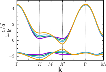
Figure 3: Band structure (19) of the noninteracting hopping term (2) with the additional staggered on-site energy term (22) (in units of the nearest-neighbor hopping amplitude $t_{1}$) along paths in the first Brillouin zone for the next-nearest-neighbor hopping amplitude $t_{2}=0.3155\,t_{1}$, phase $\phi=0.656$, and staggered on-site energy $M=0$ (magenta), $0.1$ (green), $0.2$ (blue), and $0.3\,t_{1}$ (orange).

II.2 Staggered on-site energy term

An additional interesting term, that is also present in Haldane’s original model haldane1988model , is a staggered on-site energy term that breaks inversion-symmetry:

$$H_{M}=M\sum_{i\sigma}\left(c_{iA\sigma}^{\dagger}c_{iA\sigma}-c_{iB\sigma}^{\dagger}c_{iB\sigma}\right).$$ (22)

For $|M/t_{2}|<3\sqrt{3}|\sin\phi|$, it was shown that the electronic bands are topologically nontrivial haldane1988model . Later, considering a topological Uhlmann number to characterize symmetry-protected topological phases at finite temperatures, it was verified that such a topological phase is stable up to some critical temperature $T_{c}$ delgado14 .

Adding the staggered on-site energy term (22) to the tight-binding model (2), one easily finds that the new Hamiltonian $H_{0}+H_{M}$ also assumes the form (8) with the $B_{0,{\bf k}}$ and the $B_{i,{\bf k}}$ ($i=1,2,3$) functions given by Eq. (15) apart from the replacement

$$B_{3,\mathbf{k}}\rightarrow B_{3,\mathbf{k}}+M.$$ (23)

In Fig. 3, we plot the band structure (19) for the parameters (21) and $M=0$, $0.1$, $0.2$, and $0.3\,t_{1}$. We notice that, for a finite on-site energy $M>0$ ($M<0$), the energy gap is located at the $K^{\prime}$ ($K$) point. Moreover, as the parameter $M$ increases, the energy gap decreases, the difference ($\omega^{c}_{K^{\prime}}-\omega^{c}_{K}$) increases, and the flatness ratio of the lower band $c$ decreases. Indeed, the increasing of the parameter $M$ can induce a gap closure that destroys the topological phase, see Fig. 2 from Ref. haldane1988model .

In Sec. IV.3 below, we consider a finite staggered on-site energy $M$ as a source of departure of the lower band $c$ from the nearly flat-band limit (21).

II.3 Hubbard term in momentum space

The expression of the on-site Hubbard interaction (2) easily follows from the Fourier transform of the electron density operator (6), which is given by

$$\hat{\rho}_{ia\sigma}=\frac{1}{N}\sum_{{\bf q}\in{\rm BZ}}e^{i\mathbf{q}\cdot\mathbf{R}_{i}}\hat{\rho}_{a\sigma}({\bf q}).$$ (24)

Substituting Eq. (24) into the Hamiltonian (2), one finds

$$H_{U}=\frac{1}{N}\sum_{a=A,B}\sum_{\bf q}U_{a}\hat{\rho}_{a\uparrow}(-{\bf q})\hat{\rho}_{a\downarrow}({\bf q}).$$ (25)

It is also useful to determine the expansion of the density operator $\hat{\rho}_{a\sigma}({\bf k})$ in terms of the fermion operators $c_{{\bf k}\,a\,\sigma}$. With the aid of Eqs. (6), (7), and (24), one shows that

$$\hat{\rho}_{a\sigma}({\bf q})=\sum_{\bf p}c^{\dagger}_{{\bf p}-{\bf q}\,a\,\sigma}c_{{\bf p}\,a\,\sigma}.$$ (26)

The canonical transformation (16) allows us to express (26) in terms of the fermion operators $c_{{\bf k}\,\sigma}$ and $d_{{\bf k}\,\sigma}$. In particular, the density operator (26) projected into the lower noninteracting band $c$ reads doretto2015flat

$$\bar{\rho}_{a\,\sigma}({\bf q})=\sum_{\bf p}G_{a}({\bf p},{\bf q})c^{\dagger}_{{\bf p}-{\bf q}\,\sigma}c_{{\bf p}\,\sigma},$$ (27)

with the $G_{a}({\bf p},{\bf q})$ function given by Eq. (59).

Once the expression of the projected density operator (27) is known, we can determine the projection $\bar{H}_{U}$ of the on-site Hubbard term (25) into the noninteracting lower bands $c$. Indeed, $\bar{H}_{U}$ assumes the form (25) with the replacement $\hat{\rho}_{a\sigma}({\bf q})\rightarrow\bar{\rho}_{a\sigma}({\bf q})$, i.e.,

$$\bar{H}_{U}=\frac{1}{N}\sum_{a=A,B}\sum_{\bf q}U_{a}\bar{\rho}_{a\uparrow}(-{\bf q})\bar{\rho}_{a\downarrow}({\bf q}).$$ (28)

III Bosonization formalism for flat-band Chern insulators

In this section, we briefly summarize the bosonization scheme for a Chern insulator introduced in Ref. doretto2015flat for the description of the flat-band ferromagnetic phase of a correlated Chern insulator on a square lattice.

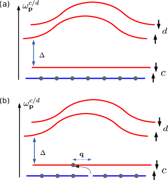
Figure 4: Schematic representation of (a) the ground state (29) of the noninteracting term (2) in the nearly-flat limit (21) of the lower band $c$ at $1/4$-filling and (b) the particle-hole pair excitation above the ground state (29). Although the free bands $c$ and $d$ are doubly degenerated with respect to the spin degree of freedom, an offset between the $\sigma=\uparrow$ and $\downarrow$ bands are introduced for clarity.

Let us consider a spinfull Chern insulator on a bipartite lattice whose Hamiltonian assumes the form (8). We choose the model parameters such that (at least) the lower band $c$ is (nearly-) flat and consider that the number of electrons $N_{e}=N_{A}=N_{B}=N$, where $N_{A}$ and $N_{B}$ are, respectively, the number of sites of the sublattices $A$ and $B$. Such a choice corresponds to a $1/4$-filling, i.e., the lower (nearly-flat) band $c$ is half-filled. In particular, let us assume that the lower band $c\,\uparrow$ is completely occupied, as illustrated in Fig. 4(a). In this case, the ground state of the noninteracting system (the reference state) is completely spin polarized and it can be written as a product of single particle states,

$$|{\rm FM}\rangle=\prod_{\mathbf{k}\in BZ}c_{\mathbf{k}\uparrow}^{\dagger}|0\rangle.$$ (29)

Since the lower flat bands $c$ are separated from the upper bands $d$ by an energy gap, the lowest-energy neutral excitations above the ground state (29) are given by particle-hole pairs within the lower bands $c$, i.e., they are spin-flips that can be written as [see Fig. 4(b)]

$$|\Psi_{\mathbf{k}}\rangle\propto S_{\bf k}^{-}|{\rm FM}\rangle.$$ (30)

It is possible to show that such particle-hole pair excitations can be treated approximated as bosons. Indeed, one can define the boson operators

$$b_{\alpha,\mathbf{q}} =\frac{\bar{S}_{-\mathbf{q},\alpha}^{+}}{F_{\alpha\alpha,\mathbf{q}}}=\frac{1}{F_{\alpha\alpha,\mathbf{q}}}\sum_{\mathbf{p}}g_{\alpha}(\mathbf{p},-\mathbf{q})c_{\mathbf{p+q}\uparrow}^{\dagger}c_{\mathbf{p}\downarrow},$$

$$b_{\alpha,\mathbf{q}}^{\dagger} =\frac{\bar{S}_{\mathbf{q},\alpha}^{-}}{F_{\alpha\alpha,\mathbf{q}}}=\frac{1}{F_{\alpha\alpha,\mathbf{q}}}\sum_{\mathbf{p}}g_{\alpha}(\mathbf{p},\mathbf{q})c_{\mathbf{p-q}\downarrow}^{\dagger}c_{\mathbf{p}\uparrow},$$ (31)

with $\alpha=0,1$, that satisfy the canonical commutation relations

$$[b_{\alpha,\mathbf{k}},b_{\beta,\mathbf{q}}^{\dagger}] =\delta_{\alpha,\beta}\;\delta_{\mathbf{k},\mathbf{q}},$$

$$[b_{\alpha,\mathbf{k}},b_{\beta,\mathbf{q}}] =[b_{\alpha,\mathbf{k}}^{\dagger},b_{\beta,\mathbf{q}}^{\dagger}]=0,$$ (32)

and whose vacuum state is given by the (reference) spin-polarized state (29), i.e.,

$$b_{\alpha,{\bf q}}|{\rm FM}\rangle=0.$$ (33)

Here the operators $\bar{S}_{{\bf q},\alpha}^{\pm}$ are linear combinations of projected spin operators associated with sublattices $A$ and $B$,

$$\bar{S}_{{\bf q},\alpha}^{\pm}=\bar{S}_{{\bf q},A}^{\pm}+(-1)^{\alpha}\bar{S}_{{\bf q},B}^{\pm},$$ (34)

with $\alpha=0,1$ and $\bar{S}^{\pm}_{{\bf q},a}=\bar{S}^{x}_{{\bf q},a}\pm i\bar{S}^{y}_{{\bf q},a}$. The operator $\bar{S}^{\lambda}_{{\bf q},a}$, with $\lambda=x,y,z$, is the $\lambda$-component of the spin operator $S^{\lambda}_{{\bf q},a}$ projected into the lower bands $c$ with $S^{\lambda}_{{\bf q},a}$ being the Fourier transform of the spin operator $S^{\lambda}_{i,a}$ at site $i$ of the sublattice $a$. Indeed, the projected operator $\bar{S}^{\lambda}_{{\bf q},a}$ is determined from $S^{\lambda}_{i,a}$ following the same procedure outlined in Sec. II.3 for the density operator (27). Finally, the $F_{\alpha\beta,\mathbf{q}}$ function is given by

$$F_{\alpha\beta,\mathbf{q}}^{2}=\sum_{\bf p}\>g_{\alpha}(\mathbf{p},\mathbf{q})g^{*}_{\beta}(\mathbf{p},\mathbf{q}),$$ (35)

with the $g_{\alpha}(\mathbf{p},\mathbf{q})$ function being related to the coefficients (17) of the canonical transformation (16),

$$g_{\alpha}(\mathbf{p},\mathbf{q})=v_{\mathbf{p}-\mathbf{q}}^{*}v_{\mathbf{p}}+(-1)^{\alpha}u_{\mathbf{p}-\mathbf{q}}^{*}u_{\mathbf{p}}.$$ (36)

Any operator expanded in terms of the fermion operators $c^{\dagger}_{{\bf k}\sigma}$ and $c_{{\bf k}\sigma}$ can, in principle, be rewritten in terms of the bosons (31). In particular, the density operator (27) projected into the lower bands $c$ assumes the form

$$\bar{\rho}_{a\sigma}(\mathbf{k}) =\frac{1}{2}N\delta_{\sigma,\uparrow}\delta_{\mathbf{k},0}+\sum_{\alpha,\beta}\sum_{\mathbf{q}}\>\mathcal{G}_{\alpha\beta a\sigma}(\mathbf{k},\mathbf{q})b_{\beta,\mathbf{k}+\mathbf{q}}^{\dagger}b_{\alpha,\mathbf{q}},$$ (37)

where the $\mathcal{G}_{\alpha\beta a\sigma}({\bf k},{\bf q})$ function is given by Eq. (LABEL:Gcal). Importantly, both $F_{\alpha\beta,\mathbf{q}}^{2}$ and $\mathcal{G}_{\alpha\beta a\sigma}({\bf k},{\bf q})$ functions can be explicitly written in terms of the coefficients (15), see Eqs. (57) and (60), respectively.

IV Flat-band ferromagnetism in the Haldane-Hubbard model

In the completely flat-band limit (band width $W_{c}=0$) of the lower noninteracting bands $c$, Hund’s rule yields that the ground state of the Haldane-Hubbard model is ferromagnetic, once such bands are half-filled note03 . As the amplitude $t_{2}$ of the next-nearest-neighbor hopping is modified and the noninteracting bands $c$ get more dispersive, the ferromagnetic phase might be stable up to a critical band width $W_{c,critic}$, for fixed on-site repulsion energies $U_{a}$ note04 . Indeed, recent exact diagonalization calculations gu2019itinerant indicate the stability of the flat-band ferromagnetic phase for the Haldane-Hubbard model in the vicinity of the nearly flat-band limit (21), see discussion below.

In this section, we study the flat-band ferromagnet phase of the Haldane-Hubbard model (1) within the bosonization formalism doretto2015flat for flat-band Chern insulators. In particular, we concentrate on the determination of the dispersion relation of the elementary (neutral) particle-hole pair excitations, i.e., we calculate the spectrum of the spin-wave excitations above the (flat-band) ferromagnetic ground state (29). We show that the spin-wave spectrum has a Goldstone mode at momentum ${\bf q}=0$, a feature that indicates the stability of the flat-band ferromagnetic ground state.

               

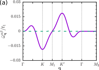
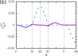
Figure 5: The real (solid magenta line) and imaginary (dashed green line) parts of (a) the coefficient $\bar{\omega}^{01}_{\bf q}$ [Eq. (41)] and (b) the coefficient $\epsilon^{01}_{\bf q}$ [Eq. (45)] along paths in the first Brillouin zone [Fig. 5(b)] for the Haldane-Hubbard model (1) in the nearly-flat band limit (21) of the lower noninteracting band $c$.

IV.1 Effective interacting boson model

Let us consider the Haldane-Hubbard model (1) on a honeycomb lattice with the noninteracting lower bands $c$ in the nearly-flat band limit (21) and at $1/4$-filling of its corresponding noninteracting limit, i.e., we assume that the number of electrons $N_{e}=N_{A}=N_{B}=N$, with $N_{A}$ and $N_{B}$ being the number of sites of the (triangular) sublattices $A$ and $B$, respectively. In this case, the bosonization scheme doretto2015flat allows us to map the Hamiltonian (1) into an effective interacting boson model.

In order to derive such an effective boson model, the first step is to project the Hamiltonian (1) into the lower noninteracting bands $c$. Such a restriction is appropriated as long as the on-site repulsion energies $U_{a}<\Delta$, where $\Delta={\rm min}(\omega_{d,{\bf k}})-{\rm max}(\omega_{c,{\bf k}})$ is the energy gap of the free-electronic bands (see Fig. 2): in particular, one finds that $\Delta=1.75\,t_{1}$ for the nearly flat-band limit (21). One shows that (see Eq. (28) from Ref. doretto2015flat for details):

$$H\rightarrow\bar{H} =\bar{H}_{0}+\bar{H}_{U}.$$ (38)

Here the projected noninteracting term $\bar{H}_{0}$ follows from Eq. (18),

$$\bar{H}_{0}=\sum_{\mathbf{k}\sigma}\omega^{c}_{\mathbf{k}}c_{\mathbf{k}\sigma}^{\dagger}c_{\mathbf{k}\sigma},$$ (39)

while the projected on-site Hubbard term $\bar{H}_{U}$ is given by Eq. (28). The expression of the noninteracting (kinetic) term $\bar{H}_{0}$ in terms of the bosons (31) is given by (see Appendix B from Ref. doretto2015flat for details)

$$\bar{H}_{0,B}=E_{0}+\sum_{\alpha\beta}\sum_{\mathbf{q}\in BZ}\bar{\omega}^{\alpha\beta}_{\mathbf{q}}b_{\beta,\mathbf{q}}^{\dagger}b_{\alpha,\mathbf{q}},$$ (40)

where $E_{0}=\sum_{\bf k}\omega^{c}_{\bf k}$ is a constant associated with the action of $\bar{H}_{0}$ into the reference state (29) and

$$\bar{\omega}^{\alpha\beta}_{\mathbf{q}} =\frac{1}{F_{\alpha\alpha,\mathbf{q}}F_{\beta\beta,\mathbf{q}}}\sum_{\mathbf{p}}\left(\omega^{c}_{\mathbf{p-q}}-\omega^{c}_{\mathbf{p}}\right)g_{\alpha}(\mathbf{p},\mathbf{q})g_{\beta}^{*}(\mathbf{p},\mathbf{q}),$$ (41)

with the $F_{\alpha\beta,\mathbf{q}}$ and the $g_{\alpha}(\mathbf{p},\mathbf{q})$ functions given by Eqs. (35) and (36), respectively. The bosonic representation of the projected on-site Hubbard term $\bar{H}_{U}$ follows from Eqs. (28) and (37): After normal ordering the expression resulting from the substitution of Eq. (37) into (28), one shows that doretto2015flat

$$\bar{H}_{U,B} =\bar{H}_{U,B}^{(2)}+\bar{H}_{U,B}^{(4)},$$ (42)

where the quadratic and quartic boson terms read

$$\bar{H}_{U,B}^{(2)} =\sum_{\alpha\beta}\sum_{\mathbf{q}}\epsilon^{\alpha\beta}_{\mathbf{q}}b_{\beta,\mathbf{q}}^{\dagger}b_{\alpha,\mathbf{q}},$$ (43)

$$\bar{H}_{U,B}^{(4)} =\frac{1}{N}\sum_{\mathbf{k},\mathbf{q},\mathbf{p}}\sum_{\alpha\beta\alpha^{\prime}\beta^{\prime}}V^{\alpha\beta\alpha^{\prime}\beta^{\prime}}_{\mathbf{k},\mathbf{q},\mathbf{p}}b_{\beta^{\prime},\mathbf{p+k}}^{\dagger}b_{\beta,\mathbf{q-k}}^{\dagger}b_{\alpha\mathbf{q}}b_{\alpha^{\prime}\mathbf{p}},$$ (44)

with the coefficient

$$\epsilon^{\alpha\beta}_{\mathbf{q}} =\frac{1}{2}\sum_{a}U_{a}\mathcal{G}_{\alpha\beta a\downarrow}(0,\mathbf{q})$$

$$+\frac{1}{N}\sum_{a,\alpha^{\prime},\mathbf{k}}U_{a}\mathcal{G}_{\alpha^{\prime}\beta a\uparrow}(-\mathbf{k},\mathbf{k+q})\mathcal{G}_{\alpha\alpha^{\prime}a\downarrow}(\mathbf{k},\mathbf{q})$$ (45)

and the boson-boson interaction given by

$$V^{\alpha\beta\alpha^{\prime}\beta^{\prime}}_{\mathbf{k},\mathbf{q},\mathbf{p}} =\frac{1}{N}\sum_{a}U_{a}\mathcal{G}_{\alpha\beta a\uparrow}(-\mathbf{k},\mathbf{q})\mathcal{G}_{\alpha^{\prime}\beta^{\prime}a\downarrow}(\mathbf{k},\mathbf{p}).$$ (46)

The effective interacting boson model that describes the flat-band ferromagnetic phase of the Haldane-Hubbard model (1) then assumes the form

$$\bar{H}_{B}=\bar{H}_{0,B}+\bar{H}^{(2)}_{U,B}+\bar{H}^{(4)}_{U,B}.$$ (47)

IV.2 Spin-wave spectrum in the nearly flat-band limit

In this section, we consider the effective boson model (47) in the lowest-order (harmonic) approximation, which consists of keeping only terms up to quadratic order in the boson operators (31) of the Hamiltonian (47), i.e., we consider

$$\bar{H}_{B} \approx\bar{H}_{0,B}+\bar{H}^{(2)}_{U,B}.$$ (48)

In principle, the Hamiltonian (48) can be diagonalized via a canonical transformation yielding the spectrum of elementary excitations (spin-waves) in terms of $\bar{\omega}^{\alpha\beta}_{\bf q}$ [Eq. (41)] and $\epsilon^{\alpha\beta}_{\mathbf{q}}$ [Eq. (45)]. However, before proceeding, we would like to discuss both contributions in details.

The coefficient $\bar{\omega}^{\alpha\beta}_{\bf q}$ [Eq. (41)] represents the (kinetic) contribution to the energy of the elementary excitations explicitly related to the dispersion of the noninteracting (lower) bands $c$. One can see that, if the free band $c$ is completely flat ($\omega^{c}_{\bf q}=$ constant), this coefficient vanishes while, in the nearly flat-band limit, it can be finite. For the noninteracting term (2) on the honeycomb lattice in the nearly flat-band limit (21), we find that $\bar{\omega}^{\alpha\alpha}_{\bf q}=0$ while $\bar{\omega}^{01}_{\bf q}=\bar{\omega}^{10}_{\bf q}$ are finite but rather small in units of the nearest-neighbor hopping energy $t_{1}$ [see Fig. 5(a)]. Such a result is distinct from the square lattice $\pi$-flux model, where symmetry considerations yield $\bar{\omega}^{\alpha\beta}_{\bf q}=0$ doretto2015flat . We believe that the finite values of the coefficients $\bar{\omega}^{01}_{\bf q}$ and $\bar{\omega}^{10}_{\bf q}$ for the Haldane model might be related not only to the symmetries of the noninteracting Hamiltonian (2), but also to the fact that the condition

$$F_{\alpha\beta,{\bf q}}=\delta_{\alpha,\beta}F_{\alpha\alpha,{\bf q}}$$ (49)

is not fulfilled for the Haldane model, an important feature distinct from the square lattice $\pi$-flux model. We refer the reader to Appendix B for a detailed discussion about the implications of the condition (49) for the approximations involved in the bosonization scheme. Due to the smallness of $\bar{\omega}^{01}_{\bf q}$ and $\bar{\omega}^{10}_{\bf q}$, in the following, we assume that $\bar{\omega}^{\alpha\beta}_{\bf q}\approx 0$, i.e., we neglected the (explicit) kinetic contribution (41) to the energy of the elementary excitations.

Concerning the coefficients (45), which are related to the one-site Hubbard term (3), we find that $\epsilon^{\alpha\alpha}_{\bf q}$ are real quantities while $\epsilon^{01}_{\bf q}=-\epsilon^{10}_{\bf q}=\epsilon^{10}_{-{\bf q}}=-\epsilon^{01}_{-{\bf q}}$ are complex ones, implying that the Hamiltonian (43) is non-Hermitian. Such a feature is also in contrast with the square lattice $\pi$-flux model doretto2015flat for which $\epsilon^{01}_{\bf q}=\epsilon^{10}_{\bf q}=0$ (see also Ref. note01 ). In particular, for the nearly flat-band limit (21), one finds that $\epsilon^{01}_{\bf q}$ is quite pronounced around the $M_{1}$ and $M_{2}$ points and it is also finite close to the $K$ and $K^{\prime}$ points of the first Brillouin zone [see Fig. 5(b)]. Again, we believe that the non-Hermiticity of the Hamiltonian $\bar{H}^{(2)}_{U,B}$ might be an artefact of the bosonization scheme related to the fact that the condition (49) is not fulfilled for the Haldane model (see Appendix B for details). Since such an issue is not completely understood at the moment, in the following, we determine the spin-wave spectrum both in the presence and in the absence of the off-diagonal terms $(\alpha,\beta)=(0,1)$ and $(1,0)$ of the Hamiltonian (43).

The Hamiltonian (48) with $\bar{\omega}^{\alpha\beta}_{\bf q}=0$ can be diagonalized via a canonical transformation similar to Eq. (16),

$$b_{0,{\bf q}}=u^{\dagger}_{\bf q}a_{+,{\bf q}}+v_{\bf q}a_{-,{\bf q}},$$

$$b_{1,{\bf q}}=v^{\dagger}_{\bf q}a_{+,{\bf q}}-u_{\bf q}a_{-,{\bf q}},$$ (50)

where the coefficients $u_{\bf q}$ and $v_{\bf q}$ are now given by

$$|u_{\bf q}|^{2},|v_{\bf q}|^{2} =\frac{1}{2}\pm\frac{1}{4\epsilon_{\bf q}}\left(\epsilon^{00}_{\bf q}-\epsilon^{11}_{\bf q}\right),$$

$$u_{\bf q}v_{\bf q}^{*} =\frac{\epsilon^{01}_{\bf q}}{4\epsilon_{\bf q}},\quad v_{\bf q}u_{\bf q}^{*}=\frac{\epsilon^{10}_{\bf q}}{4\epsilon_{\bf q}},$$ (51)

with

$$\epsilon_{\bf q}=\frac{1}{2}\sqrt{\left(\epsilon^{00}_{\bf q}-\epsilon^{11}_{\bf q}\right)^{2}+4\epsilon^{01}_{\bf q}\epsilon^{10}_{\bf q}}.$$ (52)

It is then easy to show that the Hamiltonian (48) assumes the form

$$\bar{H}_{B}=E_{0}+\sum_{\mu=\pm}\sum_{{\bf q}\in BZ}\Omega_{\mu,{\bf q}}a_{\mu,\mathbf{q}}^{\dagger}a_{\mu,\mathbf{q}},$$ (53)

where the constant $E_{0}=\sum_{\bf k}\omega^{c}_{\bf k}=(-1.69\,t_{1})N$ for the nearly flat-band limit (21) and the dispersion relation of the bosons $a_{\pm}$ reads

$$\Omega_{\pm,{\bf q}}=\frac{1}{2}\left(\epsilon^{00}_{\bf q}+\epsilon^{11}_{\bf q}\right)\pm\epsilon_{\bf q},$$ (54)

with $\epsilon_{\bf q}$ given by Eq. (52) (see also Ref. note02 ). Assuming that $\epsilon^{01}_{\bf q}=\epsilon^{10}_{\bf q}=0$, the dispersion relation (54) reduces to

$$\Omega_{-,{\bf q}}=\epsilon^{00}_{\bf q}\quad\quad{\rm and}\quad\quad\Omega_{+,{\bf q}}=\epsilon^{11}_{\bf q},$$ (55)

since $\epsilon^{00}_{\bf q}<\epsilon^{11}_{\bf q}$.

Figure 6: The elementary excitation (spin-wave) energies of the effective boson model (47) in the harmonic approximation for the nearly-flat band limit (21): dispersion relations (54) (real part, solid green line) and (55) (solid magenta line) along paths in the first Brillouin zone [Fig. 1(b)]. The dashed blue line indicates the imaginary part of $\Omega_{+,{\bf q}}=-\Omega_{-,{\bf q}}$ [see Eq. (54)], which is multiplied by a factor of 50 for clarity. On-site repulsion energies: (a) $U_{A}=U_{B}=U$; (b) $U_{B}=0.8\,U_{A}=0.8\,U$; and (c) $U_{B}=0.6\,U_{A}=0.6\,U$.

One notices that the ground state of the Hamiltonian (53) is the vacuum (reference) state for both bosons $b_{0,1}$ and $a_{\pm}$, which corresponds to the spin-polarized ferromagnet state $|{\rm FM}\rangle$ [see Eqs. (29) and (33)]. Such a result is a first indication of the stability of a flat-band ferromagnetic phase for the Haldane-Hubbard model (1). Indeed, one expects that the ferromagnetic ground state might be stable only if $U\geq U_{c}(t_{2})$. Unfortunately, due to limitations of our bosonization scheme, at the moment, it is not possible to determine such critical $U_{c}$: recall that (see Sec. IV.2) the kinetic coefficients (41) related with the dispersion of the noninteracting bands $c$ are not included in the effective boson model (47) due to the fact that the condition (49) is not fulfilled for the Haldane model. We refer the reader to Sec. V below for a more detailed discussion about the stability of the flat-band ferromagnetic phase.

The dispersion relations (54) and (55) of the bosons $a_{\pm}$, which indeed corresponds to the spin-wave spectrum above the flat-band ferromagnetic ground state (29), for the nearly flat-band limit (21) and $U_{A}=U_{B}=U$ is shown in Fig. 6(a). Due to the absence of the kinetic coefficients (41) associated with the dispersion of the noninteracting bands $c$, one sees that the energy scale of the spin-wave spectrum is determined by the on-site repulsion energy $U$. Both spin-wave spectra (54) and (55) have two branches: the acoustic (lower) branch $\Omega_{-,{\bf q}}$ is gapless, with a Goldstone mode at the Brillouin zone center ($\Gamma$ point) and the characteristic quadratic dispersion of ferromagnetic spin-waves near the $\Gamma$ point; the optical (upper) one $\Omega_{+,{\bf q}}$ is gapped, with the lowest energy excitation at the $K$ and $K^{\prime}$ points. The presence of the Goldstone mode indicates the stability of the flat-band ferromagnetic phase. Interestingly, for the dispersion relation (55), one finds a quite small energy gap at the $K$ and $K^{\prime}$ points ($\Delta^{(K)}=\Omega_{+,K}-\Omega_{-,K}=2.01\times 10^{-3}\,U$) while the excitation spectrum (54) displays Dirac points at the $K$ and $K^{\prime}$ points. Indeed, the presence of the Dirac points is related to the fact that $\epsilon^{01}_{\bf q}$ and $\epsilon^{10}_{\bf q}$ are finite at the $K$ and $K^{\prime}$ points, see Fig. 5(b). Moreover, the fact that $\epsilon^{01}_{\bf q}=-\epsilon^{10}_{\bf q}$ yields a very small decay rate (the imaginary part of $\Omega_{\pm,{\bf q}}$) for the spin-wave excitations (54) at the border of the first Brillouin zone [see the dashed line in Fig. 6(a) and note the multiplicative factor 50].

In addition to a configuration with homogeneous on-site Hubbard energy $U_{A}=U_{B}=U$, we also consider the Haldane-Hubbard model with a sublattice dependent on-site Hubbard energy. The spin-wave spectra (54) and (55) for the nearly flat-band limit (21) and with $U_{B}=0.8\,U_{A}=0.8\,U$ and $U_{B}=0.6\,U_{A}=0.6\,U$ are shown in Figs. 6(b) and (c), respectively. One notices that both spin-wave spectra (54) and (55) have a Goldstone mode at the $\Gamma$ point, the energies of the excitations decreases as the diference $\Delta U=U_{A}-U_{B}$ increases, and the difference between the energies at the $K$ and $K^{\prime}$ points (e.g., $\Omega_{-,K}-\Omega_{-,K^{\prime}}$) also increases with $\Delta U$. For $U_{B}>U_{A}$, we find similar features, but the energy at the $K$ point is lower than the one at the $K^{\prime}$ point. Importantly, the dispersion relation (55) has a small gap at the $K$ and $K^{\prime}$ points, similar to the homogeneous case $U_{A}=U_{B}$: $\Delta^{(K)}=1.81\times 10^{-3}\,U$ ($\Delta U=0.2\,U$) and $1.61\times 10^{-3}\,U$ ($\Delta U=0.4\,U$). On the other hand, for the dispersion relation (54), a finite energy gap opens at the $K$ and $K^{\prime}$ points in contrast with the homogeneous case $\Delta U=0$. One finds that $\Delta^{(K)}=3.18\times 10^{-2}\,U$ ($\Delta U=0.2\,U$) and $6.40\times 10^{-2}\,U$ ($\Delta U=0.4\,U$). Such a finite energy gap might be related to the fact that a Hubbard term with $U_{A}\not=U_{B}$ breaks inversion symmetry. Similar to the homogeneous configuration, the spin-wave excitations (54) at the first Brillouin zone border have a finite decay rate.

Gu and collaborators gu2019itinerant performed exact diagonalization calculations and determined the spin-wave spectrum for the Haldane-Hubbard model (1) in the nearly flat-band limit (21) neglecting the dispersion of the noninteracting electronic bands, which corresponds to the approximation $\bar{\omega}^{\alpha\beta}_{\bf q}=0$ considered above. For homogeneous on-site Hubbard energies $U_{A}=U_{B}$, it was found that the spin-wave spectrum has Dirac points at the $K$ and $K^{\prime}$ points (see Fig. 2(a₁) from Ref. gu2019itinerant ) while, for a finite $\Delta U$, the energies of the excitations decrease with $\Delta U$ and energy gaps open at the $K$ and $K^{\prime}$ points (see Figs. 2(b₁) and 2(c₁) from Ref. gu2019itinerant ). Remarkably, the spin-wave spectrum (54) determined within the bosonization scheme qualitatively agrees with the numerical one, apart from the fact that the numerical results do not indicate a finite decay rate.

One should mention that the presence of Dirac points at the $K$ and $K^{\prime}$ points is not only a feature of the spin-wave spectrum of the flat-band ferromagnetic phase of the Haldane-Hubbard model. Indeed, recent exact diagonalization calculations gu21 for a topological Hubbard model on a kagome lattice also indicate such a feature in the excitation spectrum of the corresponding flat-band ferromagnetic phase when the dispersion of the (lower) noninteracting electronic band is neglected.

As mentioned above, although the non-Hermiticity of the Hamiltonian (43) (and consequently finite decay rates) might be an artefact of the bosonization scheme, the off-diagonal terms $\epsilon^{01}_{\bf q}$ and $\epsilon^{10}_{\bf q}$ of the quadratic Hamiltonian (43) should be considered in order to properly describe the spin-wave spectrum at the border of the first Brillouin zone. Therefore, in the following, we determine the spin-wave spectrum away from the nearly flat-band limit (21) with the aid of Eq. (54).

IV.3 Spin-wave spectrum away from the nearly flat-band limit

Although the main focus of our discussion is the description of the flat-band ferromagnetic phase of the Haldane-Hubbard model in the nearly-flat band limit (21), we also consider configurations such that the noninteracting band $c$ has smaller flatness ratio $f_{c}<6$. In particular, we consider the effects on the spin-wave spectrum (54) related to the increasing of the band width $W_{c}$ (decreasing of the flatness ratio $f_{c}$) of the noninteracting band $c$ due to (i) the decrease/increase of the phase $\phi$ [see Figs. 2(b) and (c)] and (ii) the presence of a staggered on-site energy term (22) in the total Hamiltonian (see Fig. 3). These perturbations furnish some clues about the stability of the flat-band ferromagnetic phase.

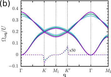
Figure 7: The real part of the dispersion relation (54) (solid line) along paths in the first Brillouin zone [Fig. 1(b)] for on-site repulsion energy $U_{A}=U_{B}=U$ and $t_{2}$ given by the relation $\cos(\phi)=t_{1}/(4t_{2})$. (a) $\phi=0.4$ (blue), $\phi=0.5$ (green), $\phi=0.656$ (magneta) and (b) $\phi=0.656$ (magneta), $\phi=0.75$ (green), $\phi=0.85$ (blue). The corresponding dashed line indicates the imaginary part of $\Omega_{+,{\bf q}}=-\Omega_{-,{\bf q}}$ [see Eq. (54)], which is multiplied by a factor of 50 for clarity.

         

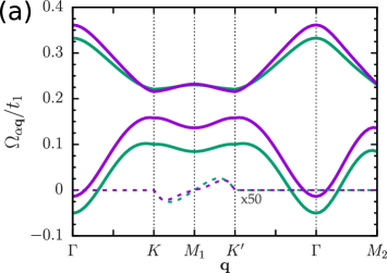
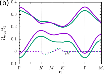
Figure 8: The real part of the dispersion relation (54) (solid line) along paths in the first Brillouin zone [Fig. 1(b)] for the optimal parameters (21), on-site Hubbard energy $U_{A}=U_{B}=U=t_{1}$, and staggered on-site energy $M=0.1$ (magenta) and $0.2\,t_{1}$ (green). (b) Similar results for the spin-wave spectrum (54), but with the replacement (56). The corresponding dashed line indicates the imaginary part of $\Omega_{+,{\bf q}}=-\Omega_{-,{\bf q}}$ [see Eq. (54)], which is multiplied by a factor of 50 for clarity.

In Fig. 7(a), we show the spin-wave spectrum (54) for $\phi=0.4$, $0.5$, and $0.656$, the hopping amplitude $t_{2}$ given by the relation $\cos(\phi)=t_{1}/(4t_{2})$, and the on-site repulsion energy $U_{A}=U_{B}=U$. One sees that the spin-wave spectrum (in units of the on-site repulsion energy $U$) for $\phi=0.4$ and $0.5$ is quite similar to the one derived for the nearly-flat band limit (21). As the flux parameter $\phi$ decreases, the excitation energies near the border of the Brillouin zone [the $K$-$M_{1}$-$K^{\prime}$ line] decrease, while the energies of the optical branch in the vicinity of the $\Gamma$ point increase. The fact that the spin-wave spectrum displays a Goldstone mode at the $\Gamma$ point, regardless the value of the phase $\phi$, indicates the stability of the flat-band ferromagnetic phase with respect to the simultaneous variations of the phase $\phi$ and the next-nearest-neighbor hopping amplitude $t_{2}$. Finite decay rates are still found at the border of the first Brillouin zone. The flat-band ferromagnetic phase seems also to be stable for $\phi>0.656$, see Fig. 7(b). Here, however, as the flux parameter $\phi$ increases, the excitation energies near the border of the Brillouin zone increase and the energies of the upper branch in the vicinity of the $\Gamma$ point decrease.

The effect on the spin-wave spectrum of a finite staggered on-site energy $M$ [Eq. (22)] is quite distinct. In Fig. 8(a), we plot the spin-wave spectrum (54) for the optimal parameters (21), $M=0.1$ and $0.2\,t_{1}$, and the on-site Hubbard energy $U_{A}=U_{B}=U=t_{1}$. Comparing with the homogeneous on-site energy $M=0$ configuration [Fig. 6(a)], one sees that the whole spin-wave spectrum shifts downward in energy as $M$ increases and energy gaps open at the $K$ and $K^{\prime}$ points. The latter is indeed related to the fact that the staggered on-site energy term (22) breaks inversion symmetry. Most importantly, the energies of the acoustic branch are negative in the vicinity of the $\Gamma$ point, indicating an instability of the flat-band ferromagnetic phase for finite values of the staggered on-site energy $M$. Such features are also found for the square lattice $\pi$-flux model doretto2015flat , see Fig. 10 in Appendix C.

A finite staggered on-site energy $M$ also modifies the (kinetic) coefficients (41) directly related to the dispersion of the noninteracting band $c$. In particular, we find that $\bar{\omega}^{\alpha\alpha}_{\bf q}$ no longer vanishes for a finite $M$ [see Fig. 5(a) for $M=0$]. Such an effect can be easily included in the spin-wave spectrum (54) with the replacement

$$\epsilon^{\alpha\alpha}_{\bf q}\rightarrow\bar{\omega}^{\alpha\alpha}_{\bf q}+\epsilon^{\alpha\alpha}_{\bf q}.$$ (56)

Figure 8(b) shows the spin-wave spectrum (54) with the replacement (56) (in units of the nearest-neighbor hopping amplitude $t_{1}$) for the optimal parameters (21), $M=0.1$ and $0.2\,t_{1}$, and the on-site Hubbard energy $U_{A}=U_{B}=U=t_{1}$. One notices that $\bar{\omega}^{\alpha\alpha}_{\bf q}$ does not modify the excitation energies in the vicinity of the $\Gamma$ point, but only changes the excitation energies near the border $K$-$M_{1}$-$K^{\prime}$ of the first Brillouin zone. Such an effect resembles the one found when distinct on-site repulsion energies $U_{A}\not=U_{B}$ are considered, see Figs. 6(b) and (c).

V Summary and discussion

The effective boson model (47) is not only restricted to the Haldane-Hubbard model (1) on a honeycomb lattice, but, in principle, it can also be employed to study the flat-band ferromagnetic phase of a correlated Chern insulator described by a topological Hubbard model on a bipartite lattice whose noninteracting (kinetic) term breaks time-reversal symmetry and assumes the form (8): Notice that a tight-binding model of the form (8) is completely defined by the $B_{0,{\bf k}}$ and $B_{i,{\bf k}}$ ($i=1,2,3$) functions (15); the $F_{\alpha\beta,{\bf q}}$ function, which is important in the definition of the boson operators (31), can be written in terms of the normalized $\hat{B}_{i,{\bf k}}=B_{i,{\bf k}}/|{\bf B}_{i,{\bf k}}|$ functions, see Eq. (57); finally, the coefficients (41) and (45) and the boson-boson interaction (46), which completely characterise the effective boson model (47), can also be expressed in terms of the normalized $\hat{B}_{i,{\bf k}}$ functions, see Appendix A.

An important requirement for the application of the bosonization scheme doretto2015flat to a topological Hubbard model is that the condition (49) is fulfilled by the noninteracting term of the model. Once the validity of such a condition is verified, the two sets of independent boson operators (31) can be defined and the bosonic representation of a operator written in terms of the original fermions, such as the projected density operator (27), is well defined. This is indeed the case for the square lattice topological Hubbard model whose noninteracting limit is giving by the $\pi$-flux model doretto2015flat . As mentioned above, the spin-wave spectrum su2019ferromagnetism determined via exact diagonalization calculations for the flat-band ferromagnetic phase of the square lattice $\pi$-flux model in the (completely) flat-band limit qualitatively agrees with the harmonic one calculated within the bosonization formalism. Additional results for the square lattice $\pi$-flux model derived within the bosonization scheme are presented in Appendix C.

For the Haldane-Hubbard model on a honeycomb lattice in the nearly-flat band limit (21) of the noninteracting (lower) band $c$ (the second application of the bosonization formalism), the condition (49) is not fulfilled for all momenta ${\bf q}$ [see Fig. 9(b)], which implies that additional considerations are needed in order to apply the bosonization scheme. As discussed in Appendix B, in order to preserve the form of the original effective boson model (47), one should assume that the two set of boson operators $b_{0,1}$ defined by Eq. (31) are independent and that the bosonic expression (37) for the projected electron density operator $\bar{\rho}_{a\sigma}({\bf k})$ holds for the Haldane model. Moreover, although the non-Hermiticity of the quadratic Hamiltonian (43) might be related to the fact that the condition (49) is not completely valid for the Haldane model, one should keep the off-diagonal terms $\epsilon^{01}_{\bf q}$ and $\epsilon^{10}_{\bf q}$ [see Eq. (45)] in order to properly describe the spin-wave excitations at the border of the first Brillouin zone (see Fig. 6) as indicated by the comparison between the dispersion relations (54) and (55) and the numerical results gu2019itinerant . Importantly, it is not clear at the moment whether the finite decay rates found for high-energy spin-wave excitations are an artefact of the bosonization scheme. Even considering these additional approximations, the qualitatively agreement between the real part of the dispersion relation (54) and the numerical spin-wave spectrum gu2019itinerant indicates that the effective boson model (47) provides an appropriated description for the flat-band ferromagnetic phase of the Haldane-Hubbard model.

In addition to the nearly-flat band limit (21), we also study the flat-band ferromagnetic phase of the Haldane-Hubbard model when the noninteracting lower band $c$ gets more dispersive. While the ferromagnetic phase seems to be less sensible to the increase of the band width $W_{c}$ of the noninteracting band $c$ due to variations of the phase $\phi$ and the next-nearest neighbor amplitude $t_{2}$ (Fig. 7), an instability of the ferromagnetic ground state is found when a staggered on-site energy (22) is included [Fig. 8(a) and (b)]. Interestingly, for the latter, one notices that the $F^{2}_{\alpha\alpha,{\bf q}}$ function and ${\rm Im}\,F^{2}_{01,{\bf q}}={\rm Im}\,F^{2}_{10,{\bf q}}$ are not affected by a finite staggered on-site energy $M$, while ${\rm Re}\,F^{2}_{01,{\bf q}}={\rm Re}\,F^{2}_{10,{\bf q}}$ acquire a constant value proportional to the staggered on-site energy $M$ [see Figs. 9(b) and (c)]: indeed, it is easy to see that the replacement (23) modifies the second term of the integrand (57), yielding an additional term proportional to the parameter $M$. Notice that the instability of a flat-band ferromagnetic phase due to a finite $M$ is also related to a stronger violation of the condition (49). At the moment, it is not clear whether such an instability is an artefact of the bosonization scheme related to some difficulties in including kinetic effects, see the discussion below. Interestingly, such kind of instability is also found for the square lattice $\pi$-flux model, see Appendix C for details.

The stability of a flat-band ferromagnetic phase was studied by Kusakabe and Aoki via exact diagonalization calculations performed for the two-dimensional Mielke model kusakabe1994ferromagnetic and Mielke and Tasaki models kusakabe1994B . A parameter $\gamma$ was introduced in the original models, such that $\gamma=0$ corresponds to (lower) noninteracting bands completely flat (flat-band limit). It was found that, for $\gamma=0$, a ferromagnetic phase is stable regardless the value of the on-site repulsion energy $U$. For finite values of the parameter $\gamma$ (system away from the flat-band limit), a ferromagnetic ground state is stable only if $U\geq U_{c}(\gamma)$ (see Figs. 1 and 2 from Ref. kusakabe1994B ). Such a scenario agrees with more recently numerical results for the square lattice $\pi$-flux model in the nearly-flat band limit su2019ferromagnetism , which indicates that a ferromagnetic phase sets in only if $U\geq U_{c}(t_{2})$, with $t_{2}$ being the next-nearest neighbor hopping amplitude. Müller et al. studied one- and two-dimensional Hubbard models with nearly-flat bands that are not in the class of Mielke and Tasaki flat-band models, since they do not obey some connectivity conditions muller16 . They found that small and moderate noninteracting band dispersion may stabilize a ferromagnetic phase for $U\geq U_{c}$, i.e., the ferromagnetic phase is driven by the kinetic energy. In particular, for a two-dimensional bilayer model, $U_{c}(\delta_{l})$ is a nonmonotonic function of the parameter $\delta_{l}$ that controls the width of the band (see Fig. 7 from muller16 ), i.e., the ferromagnetic phase sets in only for a finite band dispersion. For rigorous results about the stability of a ferromagnetic phase on Hubbard models with nearly-flat bands, we refer the reader to the review by Tasaki tasaki1996stability .

The fact that a ferromagnetic phase is stable in Hubbard models with nearly-flat (noninteracting) bands only for $U\geq U_{c}$ is related to the competition between the kinetic energy (dispersion of the noninteracting bands) and the (short-range) Coulomb interaction $U$ tasaki1996stability . The bosonization formalism doretto2015flat partially takes into account such a competition: although the explicitly contribution (41) of the dispersion of the noninteracting bands $c$ is not included in the effective boson model (47), such kinetic effects are partially considered by the bosonization scheme, since the coefficients (45) and the boson-boson interaction (46) depend on the $\hat{B}_{i,{\bf q}}$ functions (15) that completely determines the free-band structure (19). At the moment, it is not clear how to properly include in the effective boson model (47) the main effects related to the noninteracting band dispersion. Due to this limitation, we expected that the results derived within the bosonization scheme for flat-band Chern insulators get more accurate as the (lower) noninteracting bands gets less dispersive. One should recall that the bosonization scheme doretto2015flat is based on the formalism doretto2005lowest that was proposed to describe the quantum Hall ferromagnet realized in a two-dimensional electron gas at filling factor $\nu=1$: here, the noninteracting bands corresponds to (completely flat) Landau levels.

Concerning the topological properties of the spin-wave excitations, one would expect that the nontrivial topological properties of the noninteracting electronic bands of the Haldane-Hubbard model may yield a flat-band ferromagnetic phase with topologically non-trivial spin-wave excitation bands. Indeed, topological magnons in Heisenberg ferromagnets zhang13 ; malki2019topological ; owerre2016first ; owerre2016topological ; chen18 ; mook20 and, in particular, magnets on a honeycomb lattice owerre2016first ; owerre2016topological ; chen18 ; mook20 have been studied. An important ingredient for such topological magnon insulators is the Dzyaloshinskii-Moriya interaction that may open energy gaps in the magnon spectrum and yields magnon bands with nonzero Chern numbers. We calculate the Chern numbers of the spin-wave bands for configurations of the Haldane-Hubbard model whose spin-wave spectrum displays an energy gap at the $K$ and $K^{\prime}$ points [Figs. 6(b) and (c)]: we expand the Hamiltonian (48) in terms of Pauli matrices as done in Eq. (14), determine the corresponding $B_{i,{\bf q}}$ coefficients assuming that $\epsilon^{01}_{\bf q}=(\epsilon^{10}_{\bf q})^{*}$, and calculate the Chern numbers using Eq. (20). In agreement with exact diagonalization calculations (see Figs. 2(b₁) and (c₁) from gu2019itinerant ) for the Haldane-Hubbard model in the nearly flat-band limit (21) and neglecting the dispersion of the noninteracting electronic bands (similar to the approximation $\bar{\omega}^{\alpha\beta}_{\bf q}=0$ considered in Sec. IV.2), we find that the Chern numbers of the spin-wave bands vanish. Such a result is indeed a feature of the completely flat-band limit: the exact diagonalization calculations gu2019itinerant indicate that the spin-wave excitation bands have nonzero Chern numbers only when the dispersion of the noninteracting electronic bands is explicitly taking into account (see Figs. 2(a₂) and (d) from gu2019itinerant ); as discussed in the previous paragraph, at the moment, it is not clear how to include in the effective boson model (47) the main effects associated with the dispersion of the noninteracting electronic lower bands $c$.

In summary, in this paper we studied the flat-band ferromagnetic phase of a correlated Chern insulator on a honeycomb lattice described by the Haldane-Hubbard model. We considered the system at $1/4$-filling of the noninteracting bands and in the nearly-flat band limit of the noninteracting lower bands. We determined the spin-wave excitation spectrum within a bosonization scheme for flat-band correlated Chern insulators and found that it has a Goldstone mode at the first Brillouin zone center and Dirac points at the $K$ and $K^{\prime}$ points. We also studied how the spin-wave excitation spectrum changes as an offset in the on-site Hubbard energies associated with the sublattices $A$ and $B$ is introduced and as the width of the lower noninteracting bands increase due to variations of the kinetic term parameters and the presence of a staggered on-site energy term. In particular, we found that the flat-band ferromagnetic phase might be unstable when a finite staggered on-site energy term is included in the kinetic term of the Haldane-Hubbard model.

The bosonization scheme for flat-band correlated Chern insulators provides an effective interacting boson model for the description of the flat-band ferromagnetic phase of a topological Hubbard model. In the near future, we intend to study the effects of the boson-boson interaction not only in the Haldane-Hubbard model, but also in the square lattice $\pi$-flux model previously studied in Ref. doretto2015flat . Motivated by the similarities with the quantum Hall ferromagnetic phase realized in a two-dimensional electron gas at filling factor $\nu=1$ doretto2005lowest , we would like to check whether the boson-boson interaction may yield two-boson bound states.

We also intend to investigate how the bosonization scheme can be modified in order to properly include the main effects associated with the dispersion of the noninteracting electronic bands that are encoded in the kinetic coefficients $\bar{\omega}^{\alpha\beta}_{\bf q}$ [Eq. (41)]. Recall that, for the square lattice topological Hubbard model previously studied doretto2015flat , symmetry considerations yield $\bar{\omega}^{\alpha\beta}_{\bf q}=0$, while, for the Haldane model, a (small) finite $\bar{\omega}^{\alpha\beta}_{\bf q}$ might be related to the fact that the condition (49) is not fulfilled for the Haldane model. Once this is done, we will be able to properly describe flat-band ferromagnetic phases of the Haldane-Hubbard model with topologically nontrivial spin-wave excitation bands. Moreover, we could identify possible instabilities of the ferromagnetic ground state associated with a softening of the spin-wave excitation spectrum at finite momentum ${\bf q}$. Indeed, such a feature was observed in exact diagonalization calculations for a square lattice topological Hubbard model when the effects of the dispersion of the noninteracting electronic bands are explicitly taken into account (see Fig. 5 from Ref. su2019ferromagnetism ). A softening of the spin-wave bands at finite momentum ${\bf q}$ indicates that the Haldane-Hubbard model at $1/4$-filling may display other magnetic ordered phases, such as a chiral tetrahedron ordered state that was discussed in a previous mean-field analysis of the Hubbard model on a honeycomb lattice li12 . Importantly: in principle, the bosonization scheme could not be employed to study such distinct magnetic ordered phases, since the definition of the bosons operators (31) is based on the ferromagnetic (reference) state (29).

It would be interesting to see whether the bosonization formalism doretto2015flat , eventually combined with the approximations discussed in this paper, can also be employed to study twisted bilayer graphene near a magic angle cao2018unconventional ; lu19 ; sharpe19 ; morell10 ; xu18 ; wu18 ; seo19 ; sau20 ; repellin20 ; chen20 . Here the resulting moiré pattern induces an effective superlattice and a set of flat-minibands in the moiré Brillouin zone. In addition to a superconducting phase cao2018unconventional ; lu19 , evidences for a ferromagnetic phase at $3/4$-filling of the conduction miniband are also found sharpe19 . In principle, a possible flat-band ferromagnetic phase of the effective lattice model introduced in Ref. seo19 for twisted bilayer graphene could be studied within the bosonization scheme. It would be interesting to compare such results with recent numerical ones obtained within exact diagonalization sau20 ; repellin20 .

Finally, we should mention that a similar study reported in this paper for a correlated flat-band Z₂ topological insulator on a honeycomb lattice, described by a topological Hubbard model similar to Eq. (1) but that preserves time-reversal symmetry, is currently in progress and it will be published elsewhere. For $\phi=\pi/2$, such a model corresponds to the Kane-Mele-Hubbard model, see Ref. rpp-rachel18 for details.

         

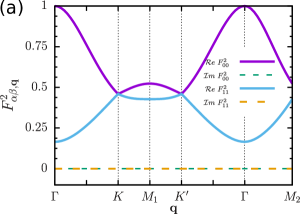
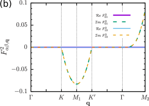
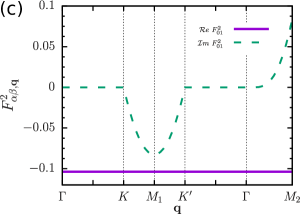
Figure 9: The real (solid line) and imaginary (dashed line) parts of the $F_{\alpha\beta,{\bf q}}^{2}$ function [Eq. (35)] for the Haldane model (2) in the nearly-flat band limit (21): (a) $F_{00,{\bf q}}^{2}$ and $F_{11,{\bf q}}^{2}$ (b) $F_{01,{\bf q}}^{2}$ and $F_{10,{\bf q}}^{2}$ for staggered on-site energy $M=0$; (c) $F_{01,{\bf q}}^{2}$ for staggered on-site energy $M=0.2\,t_{1}$.

Appendix A Expressions of the $F_{\alpha\beta,\mathbf{q}}$ and $\mathcal{G}_{\alpha\beta a\sigma}({\bf k},{\bf q})$ functions

In this section, we quote the expansions of the $F_{\alpha\beta,\mathbf{q}}$ and $\mathcal{G}_{\alpha\beta a\sigma}({\bf k},{\bf q})$ functions in terms of the coefficients (15) that were derived in Ref. doretto2015flat .

The $F_{\alpha\beta,\mathbf{q}}$ function (35) is defined in terms of the $g_{\alpha}({\bf p},{\bf q})$ function (36), which is written in terms of the coefficients $u_{\bf k}$ and $v_{\bf k}$ of the canonical transformation (16). With the aid of Eq. (17), one shows that

$$F^{2}_{\alpha\beta,{\bf q}} =\frac{1}{4}\sum_{\bf p}\left[1+(-1)^{\alpha+\beta}\right]\left(1+\hat{B}_{3,{\bf p}}\hat{B}_{3,{\bf p}-{\bf q}}\right)-\left[1-(-1)^{\alpha+\beta}\right]\left(\hat{B}_{3,{\bf p}}+\hat{B}_{3,{\bf p}-{\bf p}}\right)$$

$$+\left[(-1)^{\alpha}+(-1)^{\beta}\right]\left(\hat{B}_{1,{\bf p}}\hat{B}_{1,{\bf p}-{\bf q}}+\hat{B}_{2,{\bf p}}\hat{B}_{2,{\bf p}-{\bf q}}\right)+i\left[(-1)^{\alpha}-(-1)^{\beta}\right]\left(\hat{B}_{1,{\bf p}}\hat{B}_{2,{\bf p}-{\bf q}}-\hat{B}_{2,{\bf p}}\hat{B}_{1,{\bf p}-{\bf q}}\right),$$ (57)

with $\alpha,\beta=0,1$ and $\hat{B}_{i,{\bf k}}=B_{i,{\bf k}}/|\mathbf{B}_{\bf k}|$.

The $\mathcal{G}_{\alpha\beta a\sigma}({\bf k},{\bf q})$ function, which determines the bosonic expression (37) of the projected density operator $\bar{\rho}_{a\sigma}({\bf k})$, is defined as

$$\mathcal{G}_{\alpha\beta a\uparrow}(\mathbf{k},\mathbf{q}) = -\sum_{\mathbf{p}}\frac{G_{a}(\mathbf{p},\mathbf{k})}{F_{\alpha\alpha,\mathbf{q}}F_{\beta\beta,\mathbf{k+q}}}g_{\alpha}(\mathbf{p-k},\mathbf{q})g_{\beta}^{*}(\mathbf{p},\mathbf{k+q}),$$

$$\mathcal{G}_{\alpha\beta a\downarrow}(\mathbf{k},\mathbf{q}) = +\sum_{\mathbf{p}}\frac{G_{a}(\mathbf{p-q},\mathbf{k})}{F_{\alpha\alpha,\mathbf{q}}F_{\beta\beta,\mathbf{k+q}}}g_{\alpha}(\mathbf{p},\mathbf{q}),g_{\beta}^{*}(\mathbf{p},\mathbf{k+q}),$$

where

$$G_{a}(\mathbf{p},\mathbf{q})=\delta_{a,A}v_{\mathbf{p}-\mathbf{q}}^{*}v_{\mathbf{p}}+\delta_{a,B}u_{\mathbf{p}-\mathbf{q}}^{*}u_{\mathbf{p}}.$$ (59)

with $u_{\bf k}$ and $v_{\bf k}$ being the coefficients of the canonical transformation (16). It is then possible to show that

$$\mathcal{G}_{\alpha\beta a\uparrow}(\mathbf{k},\mathbf{q})= -\frac{1}{8}[\delta_{a,A}+\delta_{a,B}(-1)^{\alpha+\beta}]\frac{1}{F_{\alpha,\mathbf{q}}F_{\beta,\mathbf{k+q}}}$$

$$\times\sum_{p}1-3(-1)^{a}\hat{B}_{3,\mathbf{p}}+\hat{B}_{3,\mathbf{p-q}}\hat{B}_{3,\mathbf{p+k}}+\hat{B}_{3,\mathbf{p-q}}\hat{B}_{3,\mathbf{p}}+\hat{B}_{3,\mathbf{p+k}}\hat{B}_{3,\mathbf{p}}-(-1)^{a}\hat{B}_{3,\mathbf{p-q}}\hat{B}_{3,\mathbf{p}}\hat{B}_{3,\mathbf{p+k}}$$

$$+(-1)^{\alpha}[\hat{B}_{1,\mathbf{p-q}}\hat{B}_{1,\mathbf{p}}+\hat{B}_{2,\mathbf{p-q}}\hat{B}_{2,\mathbf{p}}+i(-1)^{a}(\hat{B}_{1,\mathbf{p-q}}\hat{B}_{2,\mathbf{p}}-\hat{B}_{2,\mathbf{p-q}}\hat{B}_{1,\mathbf{p}})][1-(-1)^{a}\hat{B}_{3,\mathbf{p+k}}]$$

$$+(-1)^{\beta}[\hat{B}_{1,\mathbf{p-q}}\hat{B}_{1,\mathbf{p+k}}+\hat{B}_{2,\mathbf{p-q}}\hat{B}_{2,\mathbf{p+k}}-i(-1)^{a}(\hat{B}_{1,\mathbf{p-q}}\hat{B}_{2,\mathbf{p+k}}-\hat{B}_{2,\mathbf{p-q}}\hat{B}_{1,\mathbf{p+k}}][1-(-1)^{a}\hat{B}_{3,\mathbf{p}}]$$

$$+(-1)^{\alpha+\beta}[\hat{B}_{1,\mathbf{p+k}}\hat{B}_{1,\mathbf{p}}+\hat{B}_{2,\mathbf{p+k}}\hat{B}_{2,\mathbf{p}}+i(-1)^{a}(\hat{B}_{1,\mathbf{p+k}}\hat{B}_{2,\mathbf{p}}-\hat{B}_{2,\mathbf{p+k}}\hat{B}_{1,\mathbf{p}})][1+(-1)^{a}\hat{B}_{3,\mathbf{p-q}}].$$ (60)

The expansion of the $\mathcal{G}_{\alpha\beta a\downarrow}({\bf k},{\bf q})$ function easily follows from Eq. (60), since $\mathcal{G}_{\alpha\beta a\downarrow}({\bf k},{\bf q})=-\mathcal{G}^{*}_{\alpha\beta a\uparrow}(-{\bf k},-{\bf q})$.

Appendix B Details about the bosonization scheme

In this section, we provide some details about the definition of the boson operators (31) and discuss the differences between the application of the bosonization formalism for the Haldane model and the square lattice $\pi$-flux model doretto2015flat . Indeed, the application of the bosonization scheme doretto2015flat for the Haldane model on a honeycomb lattice requires further approximations as compare to the case of the square lattice $\pi$-flux model.

           

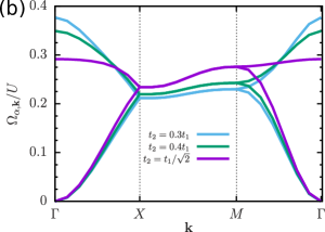
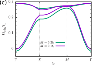
Figure 10: Spin-wave excitation spectra (54) for the flat-band ferromagnetic phase of the square lattice $\pi$-flux model (see Ref. doretto2015flat for details): (a) Next-nearest-neighbor hopping amplitudes $t_{2}=1/\sqrt{2}$ and on-site repulsion energy $U_{B}=0.8U_{A}=0.8\,U$ (magenta) and $U_{B}=0.6U_{A}=0.6\,U$ (green); (b) $U_{A}=U_{B}=U$ and $t_{2}=1/\sqrt{2}$ (magenta), $0.4$ (green), and $0.3\,t_{1}$ (blue); (c) $t_{2}=1/\sqrt{2}$, $U_{A}=U_{B}=U$, and staggered on-site energy $M=0.1$ (magenta) and $0.2\,t_{1}$ (green).

As mentioned in Sec. III, the boson operators (31) are defined in terms of projected spin operators in momentum space:

$$b_{\alpha,\mathbf{q}}\propto\bar{S}_{-\mathbf{q},\alpha}^{+}\quad\quad{\rm and}\quad\quad b_{\alpha,\mathbf{q}}^{\dagger}\propto\bar{S}_{\mathbf{q},\alpha}^{-}.$$

In terms of the fermion operators $c^{\dagger}_{{\bf k}\,\sigma}$ and $c_{{\bf k}\,\sigma}$ (associated with the lower noninteracting band $c$), the commutator between the projected spin operators $\bar{S}_{-\mathbf{q},\alpha}^{+}$ and $\bar{S}_{\mathbf{q},\alpha}^{-}$ reads

$$[\bar{S}^{+}_{{\bf q},\alpha},\bar{S}^{-}_{{\bf q}^{\prime},\beta}]= \sum_{\bf p}\left[g_{\alpha}({\bf p}-{\bf q}^{\prime},{\bf q})g_{\beta}({\bf p},{\bf q}^{\prime})c^{\dagger}_{{\bf p}-{\bf q}-{\bf q}^{\prime}\,\uparrow}c_{{\bf p}\,\uparrow}\right.$$

$$-\left.g_{\alpha}({\bf p},{\bf q})g_{\beta}({\bf p}-{\bf q},{\bf q}^{\prime})c^{\dagger}_{{\bf p}-{\bf q}-{\bf q}^{\prime}\,\downarrow}c_{{\bf p}\,\downarrow}\right],$$ (61)

with the $g_{\alpha}({\bf p},{\bf q})$ function giving by Eq. (36). One sees that Eq. (61) is different from the canonical commutation relation (32) for boson operators. However, as long as we are close to the ferromagnetic state (29), i.e., the number of particle-hole pair excitations is small, one can assume that

$$c^{\dagger}_{{\bf p}-{\bf q}\,\uparrow}c_{{\bf p}\,\uparrow} \approx\langle{\rm FM}|c^{\dagger}_{{\bf p}-{\bf q}\,\uparrow}c_{{\bf p}\,\uparrow}|{\rm FM}\rangle=\delta_{{\bf q},0},$$

$$c^{\dagger}_{{\bf p}-{\bf q}\,\downarrow}c_{{\bf p}\,\downarrow} \approx\langle{\rm FM}|c^{\dagger}_{{\bf p}-{\bf q}\,\downarrow}c_{{\bf p}\,\downarrow}|{\rm FM}\rangle=0,$$ (62)

and therefore, the commutator (61) now reads

$$[\bar{\mathbf{S}}_{\mathbf{q},\alpha}^{+},\bar{\mathbf{S}}_{\mathbf{q}^{\prime},\beta}^{-}]\approx\delta_{\mathbf{q},\mathbf{-q}^{\prime}}F_{\alpha\beta,\mathbf{q}}^{2},$$ (63)

where the $F_{\alpha\beta,\mathbf{q}}$ function is defined by Eq. (35). The commutator (63) indicates that the particle-hole pair excitations (30) can be treated approximated as bosons. The bosonization formalism for flat-band Chern insulators doretto2015flat is indeed based on the assumption (62).

For the square lattice $\pi$-flux model doretto2015flat , it was found that the condition (49) holds, and therefore, Eq. (63) allows us to define two sets of independent boson operators $b_{0}$ and $b_{1}$ as done in Eq. (31). On the other hand, for the Haldane model (2) on the honeycomb lattice, the condition (49) is not fulfilled, as exemplified in Figs. 9(a) and (b) for the nearly-flat band limit (21). Since $F_{\alpha\alpha,\mathbf{q}}^{2}$ are real quantities, the imaginary parts of $F_{01,\mathbf{q}}^{2}$ and $F_{10,\mathbf{q}}^{2}$ are finite only in the vicinity of the $M_{1}$ and $M_{2}$ points, and $|F_{01,\mathbf{q}}^{2}|$, $|F_{10,\mathbf{q}}^{2}|<|F_{\alpha\alpha,\mathbf{q}}^{2}|$, we assume that, for the Haldane model, bosons operators $b_{0}$ and $b_{1}$ can still be defined by Eq. (31) and that they constitute two sets of independent boson operators.

A second important distinction between the Haldane and square lattice $\pi$-flux models is associated with the determination of the bosonic representation of operators written in terms of the fermion operators $c_{{\bf q}\,\sigma}$, such as the projected electron density operator $\bar{\rho}_{a\sigma}({\bf k})$ [Eq. (37)]. As discussed in Sec. III.B from Ref. doretto2015flat , such a procedure is based on the fact that one can define the product of fermion operators $c^{\dagger}_{{\bf p}-{\bf q}\,\downarrow}c_{{\bf p}\,\uparrow}$ in terms of the boson operators $b_{\alpha}$, i.e.,

$$c^{\dagger}_{{\bf p}-{\bf q}\,\downarrow}c_{{\bf p}\,\uparrow}\equiv\sum_{\beta}h_{\beta}({\bf p},{\bf q})b^{\dagger}_{\beta,{\bf q}}.$$ (64)

For the square lattice $\pi$-flux model, where the condition (49) holds, it is easy to see that the $h_{\beta}({\bf p},{\bf q})$ function is given by

$$h_{\beta}({\bf p},{\bf q})=\frac{1}{F_{\beta\beta,{\bf q}}}g^{*}_{\beta}({\bf p},{\bf q}),$$ (65)

since the substitution of Eqs. (64) and (65) into (31) yields

$$b_{\alpha,\mathbf{q}}^{\dagger} =\frac{1}{F_{\alpha\alpha,\mathbf{q}}}\sum_{\beta}\left[\sum_{\mathbf{p}}h_{\beta}({\bf p},{\bf q})g_{\alpha}(\mathbf{p},\mathbf{q})\right]b_{\beta,\mathbf{q}}^{\dagger}$$

$$=\frac{1}{F_{\alpha\alpha,\mathbf{q}}}\sum_{\beta}\frac{\delta_{\alpha,\beta}F^{2}_{\alpha\beta,{\bf q}}}{F_{\beta\beta,{\bf q}}}b_{\beta,\mathbf{q}}^{\dagger}=b_{\alpha,\mathbf{q}}^{\dagger},$$ (66)

see also Eq. (35). For the Haldane model on the honeycomb lattice, the choice (65) for the $h_{\beta}({\bf p},{\bf q})$ function seems to be not appropriated, since the condition (49) is no longer valid. Due to the involved expansion of the $g_{\alpha}({\bf p},{\bf q})$ function in terms of the coefficients (15) (not shown here), it is difficult to determine an $h_{\beta}({\bf p},{\bf q})$ function such that the identity (66) is satisfied. Therefore, based on the same assumptions considered in the definition of the boson operators $b_{\alpha}$ and discussed in the previous paragraph, we also assume that Eq. (65) [and consequently Eq. (37)] holds for the Haldane model.

As discussed in Sec. IV.2, one important consequence of the fact that the condition (49) is not fulfilled for the Haldane model is that the coefficients $\bar{\omega}^{01}_{\bf q}$ and $\bar{\omega}^{10}_{\bf q}$ [Eq. (41)] are finite and the coefficients (45) obey the relation $\epsilon^{01}_{\bf q}=-\epsilon^{10}_{\bf q}$, yielding a non-Hermitian quadratic boson Hamiltonian (43). It is indeed easy to understand the relation between these results once we compare the integrand of Eq. (35) with the ones of Eqs. (41) and (LABEL:Gcal): Notice that all of them depend on the product $g_{\alpha}(x,y)g^{*}_{\beta}(x^{\prime},y^{\prime})$; for $\alpha\not=\beta$, additional terms might be included in the $\mathcal{G}_{\alpha\beta a\sigma}({\bf k},{\bf q})$ function, yielding $\epsilon^{01}_{\bf q}=-\epsilon^{10}_{\bf q}$. In principle, the condition $\epsilon^{01}_{\bf q}=(\epsilon^{10}_{\bf q})^{*}$ could be restore, once an appropriated choice for the $h_{\beta}({\bf p},{\bf q})$ function were done such that the identity (66) is now verified.

Appendix C Square lattice $\pi$-flux model

In this section, we present additional results derived within the bosonization formalism for the flat-band ferromagnetic phase of the topological Hubbard model on a square lattice, whose noninteracting limit is given by the $\pi$-flux model, previously studied in Ref. doretto2015flat . We follow the lines of Secs. IV.2 and IV.3 and find that the spin-wave spectra of both square lattice $\pi$-flux and Haldane models display the same features.

           

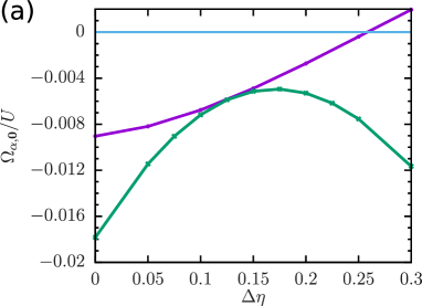
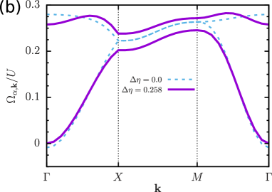
Figure 11: (a) The energy of the Goldstone mode for the square lattice $\pi$-flux model with one-site staggered energy $M=0.2\,t_{1}$ in terms of $\Delta\eta=\eta-\pi/4$ determined with the dispersion relations (54) (solid green line) and (55) (solid magenta line). (b) Dispersion relation (55) for $\Delta\eta=0$ (dashed blue line) and $\Delta\eta=0.258$ (solid magenta line).

Figure 10(a) shows the spin-wave spectrum (54) for the nearly flat-band limit of the square lattice $\pi$-flux model (which corresponds to the configuration with the next-nearest-neighbor hopping amplitude $t_{2}=t_{1}/\sqrt{2}$) and on-site repulsion energies $U_{B}=0.8\,U_{A}=0.8\,U$ and $U_{B}=0.6\,U_{A}=0.6\,U$. A comparison with the spin-wave spectrum obtained for the homogeneous case $U_{B}=U_{A}=U$ (see Fig. 4 from Ref. doretto2015flat and Fig. 10(b)) indicates that the energies of the excitations decrease with $\Delta U$ and an energy gap opens at the border of the first Brillouin zone (the $X$-$M$ line). Such features where also found for the Haldane-Hubbard model, see Fig. 6. Importantly, for the square lattice $\pi$-flux model, the decay rates of the spin-wave excitations vanish.

The effects of a decreasing of the flatness ratio of the noninteracting bands due to the variation of the next-nearest-neighbor hopping amplitude $t_{2}$ (see Fig. 3 from Ref. doretto2015flat for details) are shown in Fig. 10(b). Apart from a renormalization of the excitation energies, the spin-wave spectrum (54) display the same features of the nearly flat-band limit, similar to the behaviour found for the Haldane-Hubbard model, see Fig. 7.

Finally, the effects of a finite staggered on-site energy $M$ are presented in Fig. 10(c). Since the kinetic contribution $\bar{\omega}^{\alpha,\alpha}_{\bf q}$ is quite small it is not considered. In addition to open an energy gap at the first Brillouin zone border, a finite $M$ also decreases the lower branch energies in the vicinity of the $\Gamma$ point, which indicates an instability of the flat-band ferromagnetic phase, see also Fig. 8(a).

As discussed in Sec. V, the instability of the flat-band ferromagnetic phase in the presence of a finite staggered on-site energy $M$ might be an artefact of the bosonization formalism related to the kinetic contribution (41). Although it is not clear yet how to properly include in the effective boson model (47) the explicitly effects of the dispersion of the noninteracting bands, we check weather a modification of the boson operators (31) definition could restore the Goldstone mode. In the following, we briefly summarize such a possible procedure and apply it for the square lattice $\pi$-flux model.

The definition of the boson operators (31) is based on the linear combination (34) of the projected spin operators $\bar{S}_{\mathbf{q},A/B}$. Since a finite $M$ introduces an offset in the energies of the sites associated with the sublattices $A$ and $B$, instead of Eq. (34), one should consider the generalized form

$$\bar{S}_{\mathbf{q},0}^{\pm} =\frac{\sqrt{2}}{2}\left(\cos(\eta)\bar{S}_{\mathbf{q},A}^{\pm}+\sin(\eta)\bar{S}_{\mathbf{q},B}^{\pm}\right),$$

$$\bar{S}_{\mathbf{q},1}^{\pm} =\frac{\sqrt{2}}{2}\left(\sin(\eta)\bar{S}_{\mathbf{q},A}^{\pm}-\cos(\eta)\bar{S}_{\mathbf{q},B}^{\pm}\right),$$

where the linear combination (34) can be obtained by choosing the parameter $\eta=\pi/4$. In this case, the expansion of the $F^{2}_{\alpha\beta,{\bf q}}$ function (35) in terms of the coefficients (15) now reads

$$F_{\alpha\alpha,\mathbf{q}}^{2} =\frac{1}{4}\sum_{\mathbf{k}}[1+\hat{B}_{3\mathbf{k}}\hat{B}_{3\mathbf{k-q}}]-(-1)^{\alpha}\frac{\cos(2\eta)}{4}[\hat{B}_{3\mathbf{k}}+\hat{B}_{3\mathbf{k-q}}]+(-1)^{\alpha}\frac{\sin(2\eta)}{4}[\hat{B}_{1\mathbf{k}}\hat{B}_{1\mathbf{k-q}}+\hat{B}_{2\mathbf{k}}\hat{B}_{2\mathbf{k-q}}],$$

$$F_{\alpha\beta,\mathbf{q}}^{2} =\sum_{\mathbf{k}}-\frac{\sin(2\eta)}{4}[\hat{B}_{3\mathbf{k}}+\hat{B}_{3\mathbf{k-q}}]-\frac{\cos(2\eta)}{4}[\hat{B}_{1\mathbf{k}}\hat{B}_{1\mathbf{k-q}}+\hat{B}_{2\mathbf{k}}\hat{B}_{2\mathbf{k-q}}]-(-1)^{\alpha}\frac{i}{4}[\hat{B}_{2\mathbf{k}}\hat{B}_{1\mathbf{k-q}}-\hat{B}_{1\mathbf{k}}\hat{B}_{2\mathbf{k-q}}],$$

with $\alpha\not=\beta$, and the $g_{\alpha}({\bf p},{\bf q})$ function (36) is now given by

$$g_{\alpha}(\mathbf{p},\mathbf{q}) =G_{A}(\mathbf{p},\mathbf{q})[\cos(\eta)(1-\alpha)+\alpha\sin(\eta)]$$

$$+G_{B}(\mathbf{p},\mathbf{q})[\sin(\eta)(1-\alpha)-\alpha\cos(\eta)],$$ (69)

with the $G_{a}(\mathbf{p},\mathbf{q})$ function defined by Eq. (59). Eqs. (LABEL:newF2) and (69) implies that the expansion (60) of the $\mathcal{G}_{\alpha\beta a\sigma}({\bf k},{\bf q})$ function in terms of the coefficients (15) is also modified. Importantly, the modified $F^{2}_{\alpha\beta,{\bf q}}$ function (LABEL:newF2) with $\eta\not=\pi/4$ implies that the condition (49) is no longer valid for the square lattice $\pi$-flux model.

Figure 11(a) shows the energy of the Goldstone mode in terms of $\Delta\eta=\eta-\pi/4$ determined with both dispersion relations (54) and (55) for on-site staggered energy $M=0.2\,t_{1}$. One notices that it is possible to find a parameter $\eta$ such that the Goldstone mode is restored only if the coefficients $\epsilon^{01}_{\bf q}$ and $\epsilon^{10}_{\bf q}$ [Eq. (45)] are neglected. The spin-wave spectrum (55) for optimal $\Delta\eta=0.258$ is display in Fig. 11(b).

References

- (1) F. D. M. Haldane, Model for a Quantum Hall Effect without Landau Levels: Condensed-Matter Realization of the ”Parity Anomaly”, Phys. Rev. Lett. 61, 2015 (1988).
- (2) C. L. Kane, in Topological Insulators, Contemporary Concepts of Condensed Matter Science Vol. 6, edited by M. Franz and L. Molenkamp (Elsevier, 2013), p. 3.
- (3) S. Rachel, Interacting topological insulators: a review, Rep. Prog. Phys. 81, 116501 (2018).
- (4) X.-L. Qi and S.-C. Zhang, Topological insulators and superconductors, Rev. Mod. Phys. 83, 1057 (2011).
- (5) G. Jotzu, M. Messer, R. Desbuquois, M. Lebrat, T. Uehlinger, D. Greif, and T. Esslinger, Experimental realization of the topological Haldane model with ultracold fermions, Nature (London) 515, 237 (2014).
- (6) N. Goldman, J. C. Budich, and P. Zoller, Topological quantum matter with ultracold gases in optical lattices, Nature Phys. 12, 639 (2016).
- (7) N. R. Cooper, J. Dalibard, and I. B. Spielman, Topological bands for ultracold atoms, Rev. Mod. Phys. 91, 015005 (2019).
- (8) M. Hohenadler and F. F. Assaad, Correlation effects in two-dimensional topological insulators, J. Phys.: Condens. Matter 25, 143201 (2013).
- (9) J. He, S.-P. Kou, Y. Liang, and S. Feng, Chiral spin liquid in a correlated topological insulator, Phys. Rev. B 83, 205116 (2011).
- (10) J. He, Y.-H. Zong, S.-P. Kou, Y. Liang, and S. Feng, Topological spin density waves in the Hubbard model on a honeycomb lattice, Phys. Rev. B 84, 035127 (2011).
- (11) C. Hickey, P. Rath, and A. Paramekanti, Competing chiral orders in the topological Haldane-Hubbard model of spin- fermions and bosons, Phys. Rev. B 91, 134414 (2015).
- (12) W. Zheng, H. Shen, Z. Wang, and H. Zhai, Magnetic-order-driven topological transition in the Haldane-Hubbard model, Phys. Rev. B 91, 161107(R) (2015).
- (13) V. S. Arun, R. Sohal, C. Hickey, and A. Paramekanti, Mean field study of the topological Haldane-Hubbard model of spin- fermions, Phys. Rev. B 93, 115110 (2016).
- (14) J. Maciejko and A. Rüegg, Topological order in a correlated Chern insulator, Phys. Rev. B 88, 241101 (2013).
- (15) C. Hickey, L. Cincio, Z. Papić, and A. Paramekanti, Haldane-Hubbard Mott Insulator: From Tetrahedral Spin Crystal to Chiral Spin Liquid, Phys. Rev. Lett. 116, 137202 (2016).
- (16) T. I. Vanhala, T. Siro, L. Liang, M. Troyer, A. Harju, and P. Törmä, Topological Phase Transitions in the Repulsively Interacting Haldane-Hubbard Model, Phys. Rev. Lett. 116, 225305 (2016).
- (17) J. Wu, J. P. L. Faye, D. Sénéchal, and J. Maciejko, Quantum cluster approach to the spinful Haldane-Hubbard model, Phys. Rev. B 93, 075131 (2016).
- (18) J. Imriška, L. Wang, and M. Troyer, First-order topological phase transition of the Haldane-Hubbard model, Phys. Rev. B 94, 035109 (2016).
- (19) S. A. Parameswaran, R. Roy, S. L. Sondhi, Fractional Quantum Hall Physics in Topological Flat Bands, C. R. Phys. 14, 816 (2013).
- (20) E. J. Bergholtz and Z. Liu, Topological Flat Band Models and Fractional Chern Insulators, Int. J. Mod. Phys. B 27, 1330017 (2013).
- (21) T. Neupert, C. Chamon, T. Iadecola, L. H. Santos, and C. Mudry, Fractional (Chern and topological) insulators, Phys. Scr. 2015 014005 (2015).
- (22) T. Neupert, L. Santos, C. Chamon, and C. Mudry, Fractional Quantum Hall States at Zero Magnetic Field, Phys. Rev. Lett. 106, 236804 (2011).
- (23) K. Sun, Z. Gu, H. Katsura, and S. Das Sarma, Nearly Flatbands with Nontrivial Topology, Phys. Rev. Lett. 106, 236803 (2011).
- (24) E. Tang, J.-W. Mei, and X.-G. Wen, High-Temperature Fractional Quantum Hall States, Phys. Rev. Lett. 106, 236802 (2011).
- (25) D. N. Sheng, Z.-C. Gu, K. Sun, and L. Sheng, Fractional quantum Hall effect in the absence of Landau levels, Nature Commun. 2, 389 (2011).
- (26) N. Regnault and B. Andrei Bernevig, Fractional Chern Insulator, Phys. Rev. X 1, 021014 (2011).
- (27) B. Andrews and A. Soluyanov, Fractional quantum Hall states for moiré superstructures in the Hofstadter regime, Phys. Rev. B 101, 235312 (2020).
- (28) B. Andrews, M. Mohan, and T. Neupert, Abelian topological order of and fractional quantum Hall states in lattice models, Phys. Rev. B 103, 075132 (2021).
- (29) T. Neupert, L. Santos, S. Ryu, C. Chamon, and C. Mudry, Topological Hubbard Model and Its High-Temperature Quantum Hall Effect, Phys. Rev. Lett. 108, 046806 (2012).
- (30) R. L. Doretto and M. O. Goerbig, Flat-band ferromagnetism and spin waves in topological Hubbard models, Phys. Rev. B 92, 245124 (2015).
- (31) X.-F. Su, Z.-L. Gu, Z.-Y. Dong, S.-L. Yu, and J.-X. Li, Ferromagnetism and spin excitations in topological Hubbard models with a flat band, Phys. Rev. B 99, 014407, (2019).
- (32) For reviews on flat band ferromagnetism see, e.g., H. Tasaki, From Nagaoka’s FM to flat band FM and beyond, Prog. Theor. Phys. 99, 489 (1998); H. Tasaki, Hubbard model and the origin of ferromagnetism, Eur. Phys. J. B. 64, 365 (2008).
- (33) R. L. Doretto, A. O. Caldeira, and S. M. Girvin, Lowest Landau level bosonization, Phys. Rev. B 71, 045339, (2005).
- (34) R. L. Doretto and C. M. Smith, Quantum Hall ferromagnetism in graphene: SU (4) bosonization approach, Phys. Rev. B 76, 195431 (2007).
- (35) O. Viyuela, A. Rivas, and M. A. Martin-Delgado, Two-Dimensional Density-Matrix Topological Fermionic Phases: Topological Uhlmann Numbers, Phys. Rev. Lett. 113, 076408 (2014).
- (36) For a discussion about the stability of a ferromagnetic ground state in the completely flat-band limit of an interacting model, we refer the reader to the Supplemental Material from Ref. sau20 . More detailed discussions can be found in Refs. flat-fm ; tasaki1996stability .
- (37) For instance, the phase diagram v.s. of a square lattice topological Hubbard model was determined within exact diagonalization calculations, see Fig. 2(a) from Ref. su2019ferromagnetism : for a fixed one-site repulsion energy , it was found that the ferromagnetic ground state is stable for in the vicinity of the corresponding nearly-flat band limit.
- (38) Z.-L. Gu, Z.-Y. Dong, S.-L. Yu, J.-X. Li, Itinerant topological magnons in Haldane Hubbard model with a nearly-flat electron band, arXiv:1908.09255.
- (39) The fact that for the square lattice -flux model was not clearly stated in Ref. doretto2015flat . This feature was indeed properly taken into account, and therefore, the spin-wave spectrum shown in Fig. 4 from Ref. doretto2015flat is correct.
- (40) The diagonalization procedure employed in Ref. doretto2015flat for the harmonic Hamiltonian is not correct, and therefore, Eq. (63) from Ref. doretto2015flat is wrong. As mentioned in note01 , such a mistake does not alter the results for the square lattice -flux model derived within the bosonization scheme since .
- (41) Zhao-Long Gu1 and Jian-Xin Li, Itinerant Topological Magnons in SU(2) Symmetric Topological Hubbard Models with Nearly Flat Electronic Bands, Chin. Phys. Lett. 38, 057501 (2021).
- (42) K. Kusakabe and H. Aoki, Ferromagnetic Spin-Wave Theory in the Multiband Hubbard Model Having a flat band, Phys. Rev. Lett., 72, 144, (1994).
- (43) K. Kusakabe and H. Aoki, Robustness of the Ferromagnetism in Flat Bands, Physica B, 194, 215, (1994).
- (44) P. Müller, J. Richter, and O. Derzhko, Hubbard models with nearly flat bands: Ground-state ferromagnetism driven by kinetic energy, Phys. Rev. B 93, 144418 (2016).
- (45) H. Tasaki, Stability of ferromagnetism in Hubbard models with nearly flat bands, J. Stat. Phys. 84, 535 (1996).
- (46) L. Zhang, J. Ren, J.-S. Wang, and B. Li, Topological magnon insulator in insulating ferromagnet, Phys. Rev. B 87, 144101 (2013).
- (47) M. Malki and G.S. Uhrig, Topological magnon bands for magnonics, Phys. Rev. B 99, 174412 (2019).
- (48) S. A. Owerre, A first theoretical realization of honeycomb topological magnon insulator, J. Phys.: Condens. Matter 28, 386001, (2016).
- (49) S. A. Owerre, Topological honeycomb magnon Hall effect: A calculation of thermal Hall conductivity of magnetic spin excitations, J. Appl. Phys. 120, 043903, (2016).
- (50) L. Chen, J.-H. Chung, B. Gao, T. Chen, M. B. Stone, A. I. Kolesnikov, Q. Huang, and P. Dai Topological Spin Excitations in Honeycomb Ferromagnet CrI3, Phys. Rev. X 8, 041028 (2018).
- (51) A. Mook, K. Plekhanov, J. Klinovaja, and D. Loss, Interaction-stabilized topological magnon insulator in ferromagnets, arxiv:2011.06543.
- (52) T. Li, Spontaneous quantum Hall effect in quarter-doped Hubbard model on honeycomb lattice and its possible realization in doped graphene system, Europhys. Lett. 97, 37001 (2012).
- (53) Y. Cao, V. Fatemi, S. Fang, K. Watanabe, T. Taniguchi, E. Kaxiras, and P. Jarillo-Herrero, Unconventional superconductivity in magic-angle graphene superlattices, Nature 556, 43 (2018).
- (54) X. Lu, P. Stepanov, W. Yang, M. Xie, M. A. Aamir, I. Das, C. Urgell, K. Watanabe, T. Taniguchi, G. Zhang, A. Bachtold, Al. H. MacDonald, and D. K. Efetov, Superconductors, orbital magnets and correlated states in magic-angle bilayer graphene, Nature 574, 653 (2019).
- (55) A. L. Sharpe, E. J. Fox, A. W. Barnard, J. Finney, K. Watanabe, T. Taniguchi, M. Kastner, and D. Goldhaber-Gordon, Emergent ferromagnetism near three-quarters filling in twisted bilayer graphene, Science 365, 605 (2019).
- (56) E. Suárez Morell, J. D. Correa, P. Vargas, M. Pacheco, and Z. Barticevic, Flat bands in slightly twisted bilayer graphene: Tight-binding calculations, Phys. Rev. B 82, 121407(R) (2010).
- (57) C. Xu and L. Balents, Topological Superconductivity in Twisted Multilayer Graphene, Phys. Rev. Lett. 121, 087001 (2018).
- (58) F. Wu, A. H. MacDonald, and I. Martin, Theory of Phonon-Mediated Superconductivity in Twisted Bilayer Graphene, Phys. Rev. Lett. 121, 257001 (2018).
- (59) K. Seo, V. N. Kotov, and B. Uchoa, Ferromagnetic Mott state in Twisted Graphene Bilayers at the Magic Angle, Phys. Rev. Lett. 122, 246402 (2019).
- (60) Y. Alavirad and J. Sau, Ferromagnetism and its stability from the one-magnon spectrum in twisted bilayer graphene, Phys. Rev. B 102, 235123 (2020).
- (61) C. Repellin, Z. Dong, Y.-H. Zhang, and T. Senthil, Ferromagnetism in Narrow Bands of Moiré Superlattices, Phys. Rev. Lett. 124, 187601 (2020).
- (62) B.-B. Chen, Y. D. Liao, Z. Chen, O. Vafek, J. Kang, W. Li, and Z. Y. Meng, Realization of Topological Mott Insulator in a Twisted Bilayer Graphene Lattice Model, arxiv:2011.07602.