Discontinuous Named Entity Recognition as Maximal Clique Discovery

Abstract

Named entity recognition (NER) remains challenging when entity mentions can be discontinuous. Existing methods break the recognition process into several sequential steps. In training, they predict conditioned on the golden intermediate results, while at inference relying on the model output of the previous steps, which introduces exposure bias. To solve this problem, we first construct a segment graph for each sentence, in which each node denotes a segment (a continuous entity on its own, or a part of discontinuous entities), and an edge links two nodes that belong to the same entity. The nodes and edges can be generated respectively in one stage with a grid tagging scheme and learned jointly using a novel architecture named Mac. Then discontinuous NER can be reformulated as a non-parametric process of discovering maximal cliques in the graph and concatenating the spans in each clique. Experiments on three benchmarks show that our method outperforms the state-of-the-art (SOTA) results, with up to 3.5 percentage points improvement on F1, and achieves 5x speedup over the SOTA model.

1 Introduction

Named Entity Recognition (NER) is the task of detecting mentions of real-world entities from text and classifying them into predefined types. NER benefits many natural language processing applications (e.g., information retrieval Berger and Lafferty (2017), relation extraction Yu et al. (2019), and question answering Khalid et al. (2008)).

NER methods have been extensively investigated and researchers have proposed effective ones. Most prior approaches Huang et al. (2015); Chiu and Nichols (2016); Gridach (2017); Zhang and Yang (2018); Gui et al. (2019); Xue et al. (2020) cast this task as a sequence labeling problem where each token is assigned a label that represents its entity type. Their underlying assumption is that an entity mention should be a short span of text Muis and Lu (2016), and should not overlap with each other. While such assumption is valid for most cases, it does not always hold, especially in clinical corpus Pradhan et al. (2015). For example, Figure 1 shows two discontiguous entity mentions with overlapping segments. Thus, there is a need to move beyond continuous entities and devise methods to extract discontinuous ones.

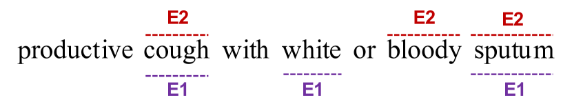
Figure 1: An example involving discontinuous mentions. Entities are highlighted with colored underlines.

Towards this goal, current state-of-the-art (SOTA) models can be categorized into two classes: combination-based and transition-based. Combination-based models first detect all the overlapping spans and then learn to combine these segments with a separate classifier Wang and Lu (2019); Transition-based models incrementally label the discontinuous spans through a sequence of shift-reduce actions Dai et al. (2020b). Although these methods have achieved reasonable performance, they continue to have difficulty with the same problem: exposure bias Zhang et al. (2019). Specifically, combination-based methods use the gold segments to guide the classifier during the training process while at inference the input segments are given by a trained model, leading to a gap between training and inference Wang and Lu (2019). For transition-based models, at training time, the current action relies on the golden previous actions, while in the testing phase, the entire action sequence is generated by the model. As a result, a skewed prediction will further deviate the predictions of the follow-up actions. Such accumulated discrepancy may hurt the performance.

In order to overcome the limitation of such prior works, we propose Mac, a Maximal clique discovery based discontinuous NER model. The core insight behind Mac is that all (potentially discontinuous) entity mentions in the sentence can naturally form a segment graph by interpreting their contained continuous segments as nodes, and connecting segments of the same entity to each other as edges. Then the discontinuous NER task is equivalent to finding the maximal cliques from the graph, which is a well-studied problem in graph theory. So, the question that remains is how to construct such a segment graph. We decompose it into two uncoupled subtasks, segment extraction (SE) and edge prediction (EP) in Mac. Typically, given an $n$-token sentence, two $n\times n$ tag tables are formed for SE and EP respectively where each entry captures the interaction between two individual tokens. SE is then regarded as a labeling problem where tags are assigned to distinguish the boundary tokens of each segment, which have benefits in identifying overlapping segments. EP is converted as the problem of aligning the boundary tokens of segments contained in the same entity. Overall, the tag tables of SE and EP are generated independently, and will be consumed together by a maximum clique searching algorithm to recover desired entities from them, thus immune from the exposure bias problem.

We conducted experiments on three standard discontinuous NER benchmarks. Experiments show that Mac can effectively recognize discontinuous entity mentions without sacrificing the accuracy on continuous mentions. This leads to a new state-of-the-art (SOTA) on this task, with substantial gains of up to 3.5% absolute percentage points over previous best reported result. Lastly, we show that in the runtime experiments on GPU environments, Mac is about five times faster than the SOTA model.

2 Related Work

Discontinuous NER requires to identify all entity mentions that have discontinuous structures. To achieve this end, several researchers introduced new position indicators into the traditional BIO tagging scheme so that the sequential labeling models can be employed Tang et al. (2013); Metke-Jimenez and Karimi (2016); Dai et al. (2017); Tang et al. (2018). However, this model suffers from the label ambiguity problem due to the limited flexibility of the extended tag set. As the improvement, Muis and Lu Muis and Lu (2016) used hyper-graphs to represent entity spans and their combinations, but did not completely resolve the ambiguity issue Dai et al. (2020b). Wang and Lu Wang and Lu (2019) presented a pipeline framework which first detects all the candidate spans of entities and then merges them into entities. By decomposing the task into two inter-dependency steps, this approach does not have the ambiguity issue, but meanwhile being susceptible to exposure bias. Recently, Dai et al. Dai et al. (2020b) constructed a transition action sequence for recognizing discontinuous and overlapping structure. At training time, it predicts with the ground truth previous actions as condition while at inference it has to select the current action based on the results of previous steps, leading to exposure bias. In this paper, for the first time we propose a one-stage method to address discontinuous NER while without suffering from the ambiguity issue, realizing the consistency of training and inference.

Joint extraction aims to detect entity pairs along with their relations using a single model Yu et al. (2020). Discontinuous NER is related to joint extraction where the discontiguous entities can be viewed as relation links between segments Wang and Lu (2019). Our model is motivated by TPLinker Wang et al. (2020), which formulates joint extraction as a token pair linking problem by aligning the boundary tokens of entity pairs. The main differences between our model and TPLinker are two-fold: (1) We propose a tailor-designed tagging scheme for recognizing discontinuous segments; (2) The maximal clique discovery algorithm is introduced into our model to accurately merge the discontinuous segments.

Maximal clique discovery is to find a clique of maximum size in a given graph Dutta and Lauri (2019). Here, a clique is a subset of the vertices all of which are pairwise adjacent. Maximal clique discovery finds extensive application across diverse domains Stix (2004); Boginski et al. (2005); Imbiriba et al. (2017). In this paper, we reformulate discontinuous NER as the task of maximal clique discovery by constructing a segment graph and leveraging the classic B-K backtracking algorithm Bron and Kerbosch (1973) to find all the maximum cliques as the entities.

3 Methodology

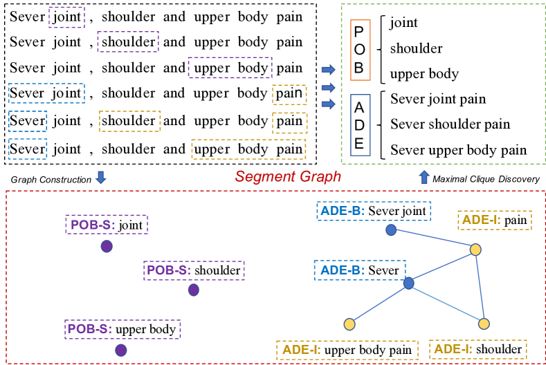
Figure 2: An example of the extraction process.

In graph theory, a clique is a vertex subset of an undirected graph where every two vertices in the clique are adjacent, while a maximal clique is the one that cannot be extended by including one more adjacent vertex. That means each vertex in the maximal clique has close relations with each other, and no other vertex can be added, which is similar to the relations between segments in a discontinuous entity. Based on this insight, we claim that discontinuous NER can be equivalently interpreted as discovering maximal cliques from a segment graph, where nodes represent segments that either form entities on their own or present as parts of a discontinuous entity, and edges connect segments that belong to the same entity mention.

Considering the maximum clique searching process is usually non-parametric Bron and Kerbosch (1973), discontinuous NER is actually decomposed into two subtasks: segment extraction and edge prediction, to respectively create the nodes and edges of the segment graph. Their prediction results can be generated independently with our proposed grid tagging scheme, and will be consumed together to construct a segment graph, so that the maximal clique discovery algorithm can be applied to recover desired entities. The overall extraction process is depicted in Figure 2. Next, we will first introduce our grid tagging scheme and its decoding workflow. Then we will detail the Mac, a Maximal clique discovery based discontinuous NER model based on this tagging scheme.

3.1 Grid Tagging Scheme

Inspired by Wang et al. (2020), we implement single-stage segment extraction and edge prediction based on a novel grid tagging scheme. Given an $n$-token sentence, our scheme constructs an $n\times n$ tag table by enumerating all possible token pairs and giving each token pair the tag(s) based on their relation(s). Note that one token pair may have multiple tags according to the pre-defined tag set.

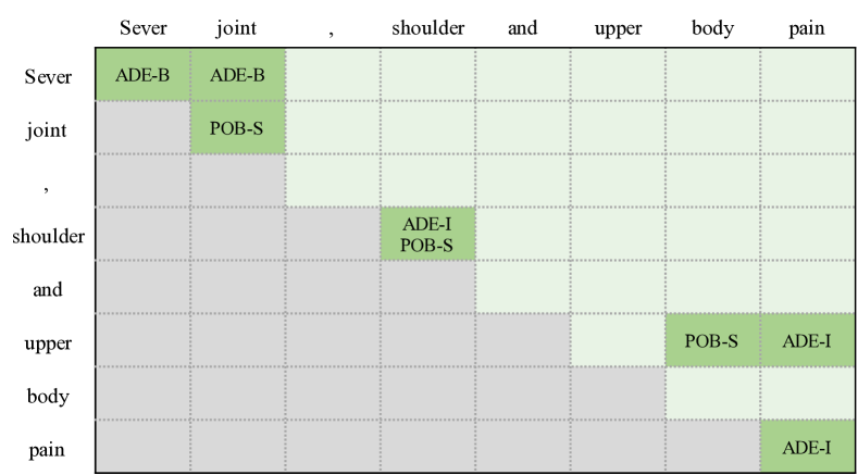
Figure 3: A tagging example for segment extraction.

3.1.1 Segment Extraction

As demonstrated in Figure 1, entity mentions could overlap with each other. To make our model capable of extracting such overlapping segments, we construct a two-dimensional tag table. Figure 3 provides an example. A pair of tokens $(t_{i},t_{j})$ will be assigned with a set of labels if a segment from $t_{i}$ to $t_{j}$ belongs to the corresponding categories. Considering $j\geq i$, we discard the lower triangle region of the tag table, so $\frac{n^{2}+n}{2}$ grids are actually generated for an $n$-token sentence. In practice, the BIS tagging scheme is adopted to represent if a segment is a continuous entity mention (X-S) or locates at the beginning (X-B) or inside (X-I) of a discontinuous entity of type X. For example, (upper, body) is assigned with the tag POB-S since “upper body” is a continuous entity of type Part of Body (POB). And the tag of (Sever, joint) is ADE-B as “Sever joint” is a beginning segment of the discontinuous mention “Sever joint pain” of type Adverse Drug Event (ADE). Meanwhile, “joint” is also recognized as an entity since there is a POB-S tag in the place of (joint, joint), thus the overlapping segment extraction problem is solved.

3.1.2 Edge Prediction

Edge prediction is to construct the links between segments of the same entity mention by aligning their boundary tokens. The tagging scheme is defined as follows: (1) head to head (X-H2H) indicates it locates in a place ($t_{i}$, $t_{j}$) where $t_{i}$ and $t_{j}$ are respectively the beginning tokens of two segments which constitute the same entity of type X; (2) tail to tail (X-T2T) is similar to X-H2H, but focusing on the ending token. As shown in Figure 4, “Sever” has the ADE-H2H and ADE-T2T relations to “shoulder” and “pain”, because the type of the discontinuous entity mention “Sever shoulder pain” is Adverse Drug Event . The same logic goes for other tags in the matrix.

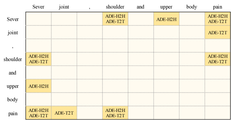
Figure 4: A tagging example for edge prediction.

3.2 Decoding Workflow

Formally, the decoding procedure is summarized in Algorithm 1. The segment tagging table $\rm S$ and edge tagging table $\rm E$ of a sentence $\rm T$ serve as the inputs. Firstly, we extract all the typed segments through decoding $\rm S$. Then we construct a segment graph $G$, in which segments that belong to the same entity (decoded from $\rm E$) have edges with each other. Figure 2 gives an example. Correspondingly, we can yield a continuous entity mention from the single-vertex clique directly, and concatenate segments in each multiple-vertex clique following their original sequential order in $\rm T$ to recover discontinuous entity mentions. We choose the classic B-K backtracking algorithm  Bron and Kerbosch (1973) for finding the maximal cliques in $G$, which takes $O(3^{\frac{m}{3}})$ time, where $m$ is the number of nodes.

Algorithm 1 Decoding Procedure

1:The segment tagging results $\rm S$ and edge tagging results $\rm E$ of sentence $\rm T$. ${\rm S}(t_{i},t_{j})$ and ${\rm E}(t_{i},t_{j})$ respectively denote the tag set of token pair $(t_{i},t_{j})$ in two schemes.

2:${\rm R}=\{(e_{k},t_{k})\}_{k=1}^{m}$, $e_{k}$, $t_{k}$ are respectively the text and the type of the $k$-th entity.

3:Initialize the edge set $\rm{A}$ and entity set $\rm{R}$ with $\varnothing$

4:Obtain the segment set $\rm{N}$ by decoding $S$.

5:for segment $s\in{\rm N}$ do

6:     for segment $g\in{\rm N}$ do

7:         Define type $\leftarrow$ the entity type of $s$ or $g$

8:         if type-H2H $\in$ E(s.start, g.start) $\And$ type-T2T $\in$ E(s.end, g.end) then

9:              Add (s, g) to $A$

10:         end if

11:     end for

12:end for

13:Construct the segment graph $G$ based on N and A

14:Find the maximal cliques $C$ in $G$ with the B-K algorithm

15:for clique $c\in C$ do

16:     Define $t\leftarrow$ the entity type of a random segment in $c$

17:     Concat the segments of $c$ with their order in $\rm T$ as $e$

18:     Add $(e,t)$ to ${\rm R}$

19:end for

20:return R

Algorithm 2 B-K Backtracking Algorithm

1:The graph $G$

2:the set of all maximal cliques: $\rm{C}$.

3:Initialize $\rm{C}$ and two vertex sets R, X with $\varnothing$

4:Define P $\leftarrow$ the node set of $G$

5:function BronKer(R, P, X)

6:     if P $=\varnothing~{}\And$ X$=\varnothing$ then

7:         Add R to $\rm{C}$

8:     end if

9:     for $v\in$ P  do

10:         Define N$(v)\leftarrow$ the neighbor set of $v$

11:         BronKer( R $\cup$ N$(v)$, P $\cap$ N$(v)$, X $\cap$ N$(v)$)

12:         P $\leftarrow$ P $\backslash$ ${v}$

13:         X $\leftarrow$ X $\cup$ ${v}$

14:     end for

15:end function

16:BronKer(R, P, X) // call the BronKer function

17:return $\rm{C}$

3.3 Model Structure

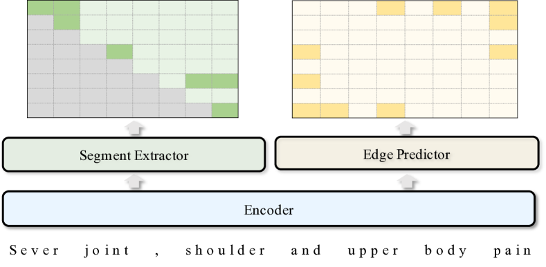
Figure 5: The overall structure of the Mac model.

With the grid tagging scheme, we propose an end-to-end neural architecture named Mac. Figure 5 reveals the overview structure.

3.3.1 Token Representation

Given an $n$-token sentence $[t_{1},\cdots,t_{n}]$, we first map each token $t_{i}$ into a low-dimensional contextual vector $\mathbf{h_{i}}$ with a basic encoder. Then we generate two representations, $\mathbf{h}^{s}_{i}$ and $\mathbf{h}^{e}_{i}$, as the task-specific features for the segment extractor and the edge predictor, respectively:

$$\mathbf{h}^{s}_{i}=\mathbf{W}^{s}_{h}\cdot\mathbf{h}_{i}+\mathbf{b}^{s}_{h},$$ (1)

$$\mathbf{h}^{e}_{i}=\mathbf{W}^{e}_{h}\cdot\mathbf{h}_{i}+\mathbf{b}^{e}_{h},$$ (2)

where $\mathbf{W}^{*}_{h}$ is a parameter matrix and $\mathbf{b}^{*}_{h}$ is a bias vector to be learned during training.

3.3.2 Segment Extractor

The probability that a pair of tokens are the boundary tokens of a segment can be represented as:

$$P(t_{i},t_{j})=P(e=t_{j}|b=t_{i})P(b=t_{i}),$$ (3)

where $b$ and $e$ denotes the beginning token and ending token. In our tagging scheme (Figure 3), we have a fixed beginning token $t_{i}$ at the $i$-th row, and take the given beginning token as the condition to label the corresponding ending token, so $P(b=t_{i})$ in the $i$-th row is always 1. Hence, all we need to do is to calculate $P(e=t_{j}|b=t_{i})$.

Inspired by Su (2019) and Yu et al. Yu et al. (2021), we levderage the Conditional Layer Normalization (CLN) mechanism to model the conditional probability. That is, a conditional vector is introduced as extra contextual information to generate the gain parameter $\gamma$ and bias $\lambda$ of the well known layer normalization mechanism Ba et al. (2016) as follows:

$${\rm CLN}(\mathbf{c},\mathbf{x})=\gamma_{c}\odot(\frac{\mathbf{x}-\mu}{\sigma})+\lambda_{c},$$ (4)

$$\mu =\frac{1}{d}\sum_{i=1}^{d}x_{i},\;\;\;\sigma=\sqrt{\frac{1}{d}\sum_{i=1}^{d}(x_{i}-\mu)^{2}},$$ (5)

$$\gamma_{c} =\mathbf{W}_{\alpha}\mathbf{c}+\mathbf{b}_{\alpha},\;\;\;\lambda_{c}=\mathbf{W}_{\beta}\mathbf{c}+\mathbf{b}_{\beta}.$$ (6)

where $\mathbf{c}$ and $\mathbf{x}$ are the conditional vector and input vector respectively. $x_{i}$ denotes the $i$-th element of $\mathbf{x}$, $\mu$ and $\sigma$ are the mean and standard deviation taken across the elements of $\mathbf{x}$, respectively. $\mathbf{x}$ is firstly normalized by fixing the mean and variance and then scaled and shifted by $\gamma_{c}$ and $\lambda_{c}$ respectively. Based on the CLN mechanism, the representation of token pair $(t_{i},t_{j})$ being a segment boundary can be defined as:

$$\mathbf{h}^{sb}_{i,j}={\rm CLN}(\mathbf{h}^{s}_{i},\mathbf{h}^{s}_{j}).$$ (7)

In this way, For different $t_{i}$, different LN parameters are generated, which results in effectively adapting $\mathbf{h}_{j}$ to be more $t_{i}$-specific.

Furthermore, besides the features of boundary tokens, we also consider inner tokens and segment length to learn a better segment representation. Specifically, we deploy a LSTM network Hochreiter and Schmidhuber (1997) to compute the hidden states of inner tokens, and use a looking-up table to embed the segment length. Since the ending token is always behind the beginning one, in each row $r_{i}$, only the tokens behind $t_{i}$ will be fed into the LSTM. We take the hidden state outputted at each time step $t_{j}$ as the inner token representation of the segment $s_{i:j}$. Then the representation of a segment from $t_{i}$ to $t_{j}$ can be defined as follows:

$$\mathbf{h}^{in}_{i:j} ={\rm LSTM}(\mathbf{h}^{s}_{i},...,\mathbf{h}^{s}_{j}),j\geq i,$$ (8)

$$\mathbf{e}^{len}_{i:j} ={\rm Emb}(j-i),j\geq i,$$ (9)

$$\mathbf{h}^{s}_{i:j} =\mathbf{h}^{sb}_{i,j}+\mathbf{h}^{in}_{i:j}+\mathbf{e}^{len}_{i:j}.$$ (10)

3.3.3 Edge Predictor

Edge prediction is similar with segment extraction since they all need to learn the representation of each token pair. The key differences are summarized in the following two aspects: (1) the distance between segments is usually not informative, so the length embedding $\mathbf{e}^{len}_{i:j}$ is valueless in edge prediction; (2) encoding the tokens between segments may carry noisy semantics for correlation tagging and aggravate the burden of training, so no $\mathbf{h}_{i:j}^{in}$ is required. Under such considerations, we represent each token pair for edge prediction as:

$$\mathbf{h}^{e}_{i,j}={\rm CLN}(\mathbf{h}^{e}_{i},\mathbf{h}^{e}_{j}).$$ (11)

3.4 Training and Inference

In practical, our grid tagging scheme aims to tag most relevant labels for each token pair, so it can be seen as a multi-label classification problem. Once having the comprehensive token pair representations ($\mathbf{h}^{s}_{i:j}$ and $\mathbf{h}^{e}_{i:j}$), we can build the multi-label classifier via a fully connected network. Mathematically, the predicted probability of each tag for $(t_{i},t_{j})$ can be estimated via:

$$\mathbf{p}^{\mathcal{I}}_{i,j}={\rm sigmoid(}\mathbf{W}^{\mathcal{I}}\cdot\mathbf{h}^{\mathcal{I}}_{i,j}+\mathbf{b}^{\mathcal{I}}),$$ (12)

where $\mathcal{I}\in\{\text{s},\text{e}\}$ is the symbol of subtask indicator, denoting segment extraction and edge prediction respectively, and each dimension of $\mathbf{p}^{\mathcal{I}}_{i,j}$ denotes the probability of a tag between $t_{i}$ and $t_{j}$. The sigmoid function is used to transfer the projected value into a probability, in this case, the cross-entropy loss can be used as the loss function which has been proved suitable for multi-label classification task:

$$\mathcal{L}^{\mathcal{I}}=- \sum_{i=1}^{n}\sum_{j=s^{\mathcal{I}}}^{n}\sum_{k=1}^{K^{\mathcal{I}}}(\mathbf{y}_{i,j}^{\mathcal{I}}[k]{\rm log}(\mathbf{p}^{\mathcal{I}}_{i,j}[k])$$ (13)

$$+(1-\mathbf{y}_{i,j}^{\mathcal{I}}[k]){\rm log}(1-\mathbf{p}^{\mathcal{I}}_{i,j}[k])),$$

where $K^{\mathcal{I}}$ is the number of pre-defined tags in $\mathcal{I}$, $\mathbf{p}^{\mathcal{I}}_{i,j}[k]\in[0,1]$ is the predicted probability of $(t_{i},t_{j})$ along the $k$-th tag, and $\mathbf{y}_{i,j}^{\mathcal{I}}[k]\in\{0,1\}$ is the corresponding ground truth. $s^{\mathcal{I}}$ equals to $1$ if $\mathcal{I}=\text{e}$ or $i$ if $\mathcal{I}=\text{s}$. Then, the losses from segment extraction and edge prediction are aggregated to form the training objective $\mathcal{J}(\theta)$:

$$\mathcal{J}(\theta)=\mathcal{L}^{\text{s}}+\mathcal{L}^{\text{e}}.$$ (14)

At inference, the probability vector $\mathbf{p}^{\mathcal{I}}_{i,j}$ needs thresholding to be converted to tags. We enumerate several values in the range $(0,1)$ and pick the one that maximizes the evaluation metrics on the validation (dev) set as the threshold.

4 Evaluation

4.1 Datasets

Following previous work Dai et al. (2020b), we conduct experiments on three benchmark datasets from the biomedical domain: (1) CADEC Karimi et al. (2015) is sourced from AskaPatient: an online forum where patients can discuss their experiences with medications. We use the dataset pre-processed by  Dai et al.Dai et al. (2020b) which selected Adverse Drug Event (ADE) annotations from the original dataset because only the ADEs involve discontinuous annotations. (2) ShARe 13 Pradhan et al. (2013) and (3) ShARe 14 Mowery et al. (2014) focus on the identification of disorder mentions in clinical notes, including discharge summaries, electrocardiogram, echocardiogram, and radiology reports. Around 10% of mentions in these three data sets are discontinuous. The descriptive statistics of the datasets are reported in Table 1.

4.2 Implementation Details

We implement our model upon the in-field BERT base model: Yelp Bert Dai et al. (2020a) for CADEC, and Clinical BERT Alsentzer et al. (2019) for ShARe 13 and 14. The network parameters are optimized by Adam Kingma and Ba (2014) with a learning rate of 1e-5. The batch size is fixed to 12. The threshold for converting probability to tag is set as 0.5. All the hyper-parameters are tuned on the dev set. We run our experiments on a NVIDIA Tesla V100 GPU for at most 300 epochs, and choose the model with the best performance on the dev set to output results on the test set. we report the test score of the run with the median dev score among 5 randomly initialized runs.

	CADEC			ShARe 13			ShARe 14
	train	dev	test	train	dev	test	train	dev	test
S	5,340	1,097	1,160	8,508	1,250	9,009	17,407	1,361	15,850
M	4,430	898	990	5,146	669	5,333	10,354	771	7,922
D	491	94	94	581	71	436	1,004	80	566
P	11.1	10.5	9.5	11.3	10.6	8.2	9.7	10.4	7.1

Table 1: Statistics of datasets. S, M, and D respectively represent the number of sentences, total mentions, and discontinuous mentions. P denotes the percentage of discontinuous mentions in total mentions.

Model	CADEC			ShARe 13			ShARe 14
	Prec.	Rec.	F1	Prec.	Rec.	F1	Prec.	Rec.	F1
BIOE	68.7	66.1	67.4	77.0	72.9	74.9	74.9	78.5	76.6
Graph	72.1	48.4	58.0	83.9	60.4	70.3	79.1	70.7	74.7
CombB	69.8	68.7	69.2	80.1	73.9	76.9	76.5	82.3	79.3
TransE	68.9	69.0	69.0	80.5	75.0	77.7	78.1	81.2	79.6
TransB	68.8	67.3	68.0	77.3	72.9	75.0	76.0	78.6	77.3
Mac	70.5	72.5	71.5	84.3	78.2	81.2	78.2	84.7	81.3

Table 2: Main results on three benchmark datasets. Bold marks highest number among all models.

4.3 Comparison Models

For comparison, we employ the following models as baselines: (1) BIOE Metke-Jimenez and Karimi (2016) expands the BIO tagging scheme with additional tags to represent discontinuous entity; (2) Graph Muis and Lu (2016) uses hyper-graphs to organize entity spans and their combinations; (3) Comb Wang and Lu (2019) first detects entity spans, then deploys a classifier to merge them. For fair comparison, we re-implement Comb based on the in-fild BERT backbone called Comb_B; (4) Trans_E Dai et al. (2020b) is the current best discontinuous NER method, which generates a sequence of actions with the aid of buffer and stack structure to detect entity; Note that the original Trans_E model is based on ELMo. For fair comparison with our model, we also implement the in-field BERT-based Trans models, namely Trans_B.

Model	CADEC			ShARe 13			ShARe 14
	Prec.	Rec.	F1	Prec.	Rec.	F1	Prec.	Rec.	F1
BIOE	68.3/ 5.8	52.0/ 1.0	57.3/ 1.8	51.8/ 39.7	39.5/ 12.3	44.8/ 18.8	37.5/ 8.8	38.4/ 4.5	37.9/ 6.0
Graph	69.5/ 60.8	43.2/ 14.8	53.3/ 23.9	82.3/ 78.4	47.4/ 36.6	60.2/ 50.0	60.0/ 42.7	52.8/ 39.5	56.2/ 41.1
CombB	63.9/ 44.0	57.8/ 23.4	60.7/ 30.6	59.7/ 65.5	49.8/ 29.6	54.3/ 40.8	52.9/ 51.2	52.8/ 35.0	52.9/ 41.6
TransE	66.5/ 41.2	64.3/ 35.1	65.4/ 37.9	70.5/ 78.5	56.8/ 39.4	62.9/ 52.5	61.9/ 56.1	64.5/ 43.8	63.1/ 49.2
TransB	69.1/ 39.5	64.4/ 34.0	66.7/ 36.6	68.2/ 65.9	55.4/ 39.0	61.1/ 49.0	55.5/ 52.0	55.6/ 37.8	55.6/ 43.8
Mac	74.7/ 52.9	65.5/ 38.3	69.8/ 44.4	77.9/ 66.1	60.5/ 48.4	68.1/ 55.9	69.3/ 51.0	70.2/ 57.6	69.7/ 54.1

Table 3: Results on discontinuous entity mentions. In the Table, two scores are reported and separated by a slash (“/”). The former is the score on sentences with at least one discontinuous entity mention. The latter is the score only considering discontinuous entity mentions.

4.4 Main results

Table 2 reports the results of our model against other baseline methods. We have the following observations. (1) Our method, Mac, significantly outperforms all other methods and achieves the SOTA F1 score on all three datasets. (2) BERT-based Trans model achieves poorer results than its ELMo-based counterpart, which is in line with the claim in the original paper. (3) Over the SOTA method Trans_E, Mac achieves substantial improvements of 2.6% in F1 score on three datasets averagely. Moreover, the Wilcoxon’s test shows that a significant difference ($p<0.05$) exists between our model and Trans_E. We consider that it is because Trans_E is inherently a multi-stage method as it introduces several dependent actions, thus suffering from the exposure bias problem. While for our Mac method, it elegantly decomposes the discontinuous NER task into two independent subtasks and learns them together with a joint model, realizing the consistency of training and inference. (4) Comb_B can be approximately seen as the pipeline version of our method, their performance gap again confirms the effectiveness of our one-stage learning framework.

As shown in Table 1, only around 10% mentions are discontinuous in all three datasets, which is far less than the continuous entity mentions. To evaluate the effectiveness of our proposed model on recognizing discontinuous mentions, following Muis and Lu (2016), we report the results on sentences that include at least one discontinuous mention. We also report the evaluation results when only discontinuous mentions are considered. The scores in these two settings are separated by a slash in Table 3. Comparing Table 2 and 3, we can see that the BIOE model performs better than the Graph when testing on the full dataset but far worse on discontinuous mentions. Consistently, our model again defeat the baseline models in terms of F1 score. Even though some models outperform Mac on precision or recall, they greatly sacrifice another score, which results in lower F1 score than Mac.

4.5 Model Ablation Study

Model	F1	Dis F1	Dis F1⋆
Mac	78.7	56.4	46.6
– Tag B and S	78.2	55.8	46.1
– Segment length embedding	78.1	55.7	46.2
– CLN mechanism	76.8	52.7	44.4
– Segment inner representation	72.9	55.6	46.3

Table 4: An ablation study on the ShARe 13 dev set. F1, Dis F1, and Dis F1^⋆ respectively denote the overall F1 score, F1 score on sentences with at least one discontinuous mention, and on discontinuous mentions.

To verify the effectiveness of each component, we ablate one component at a time to understand its impact on the performance. Concretely, we investigated the tagging scheme of segments, the segment length embedding, the CLN mechanism (by replacing it with the vector concatenation), and the segment inner token representation.

From these ablations shown in Table 4, we find that: (1) When we take B, I and S tags in segment extraction as one class, the score slightly drops by 0.5%, which indicates the segments in different positions of entities may have different semantic features, so distinguishing them can reduce the confusion in the process of model recognition; (2) When we remove the segment length embedding (Formula 9), the overall F1 score drops by 0.6%, showing that it is necessary to let segment extractor aware of the token pair distance information to filter out impossible segments by implicit distance constraint; (3) Compared with concatenating, it is a better choice to use CLN (Formula 7 and 11) to fuse the features of two tokens, which brings 1.9% improvement; (4) Removing segment inner features (Formula 8) results in a remarkable drop on the overall F1 score while little drop on the scores of discontinuous mentions, which suggests that the information of inner tokens is essential to recognize continuous entity mentions. Overall, we can conclude that the improvement of grid encoder brings significant performance gains.

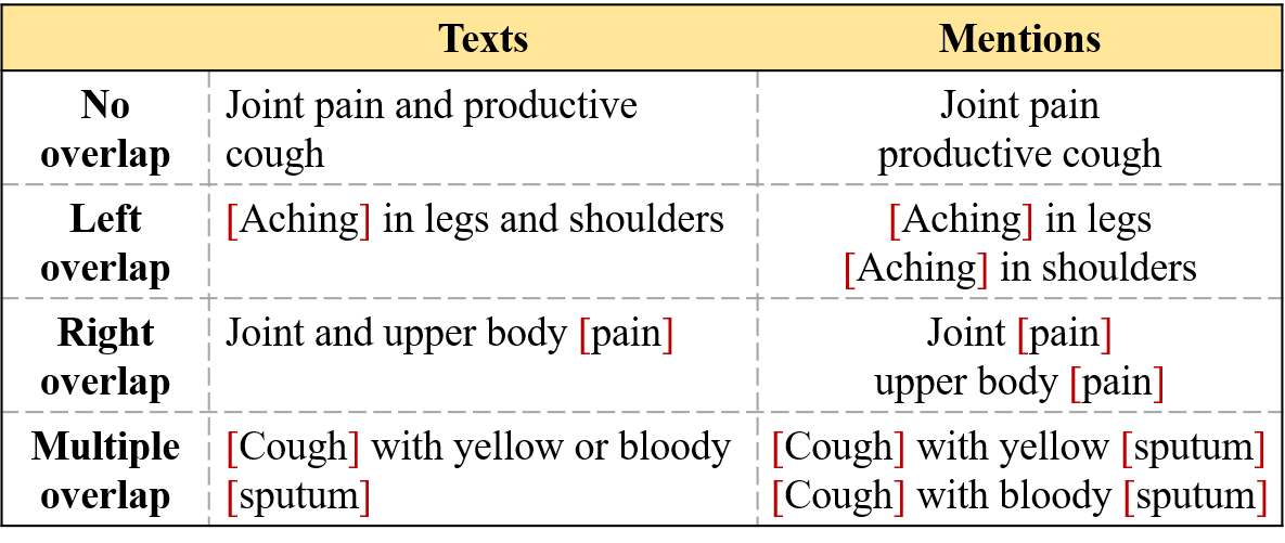
Figure 6: Examples of the overlapping patterns

Pattern	CADEC			ShARe 13			ShARe 14
	train	dev	test	train	dev	test	train	dev	test
No	57	9	16	348	41	193	535	39	246
Left	270	54	41	167	11	200	352	30	238
Right	113	16	23	48	19	35	97	5	67
Multi.	51	15	14	18	0	8	20	6	15

Table 5: Statistics of overlapping patterns.

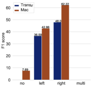
(a) CADEC

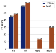
(b) ShARe 13

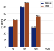
(c) ShARe 14

Figure 7: Performance on different overlapping patterns.

4.6 Performance Analysis

4.6.1 Impact of Overlapping Structure

As discussed in the introduction, overlap is very common in discontinuous entity mentions. To evaluate the capability of our model on extraction overlapping structures, as suggested in  Dai et al. (2020b), we divide the test set into four categories: (1) no overlap; (2) left overlap; (3) right overlap; and (4) multiple overlap. Figure 6 gives examples for each overlapping pattern. As illustrated in Figure 7, Mac outperforms Trans_E on all the overlapping patterns. Trans_E gets zero scores on some patterns. It might result from insufficient training since these overlapping patterns have relatively fewer samples in the training sets (see Table 5), while the sequential action structure of transition-based model is a bit data hungry. By contrast, Mac is more resilient to overlapping patterns, we attribute the performance gains to two design choices: (1) the grid tagging scheme has strong power in accurately identifying overlapping segments and assembling them into a segment graph; (2) Based on the graph, the maximal clique discovery algorithm can effectively recover all the candidate overlapping entity mentions.

4.6.2 Impact of Interval and Span Length

Length	CADEC			ShARe 13			ShARe 14
	train	dev	test	train	dev	test	train	dev	test
= 1	36	8	8	96	15	125	227	10	107
= 2	217	42	54	215	26	118	322	33	146
= 3	56	14	12	102	12	91	184	20	120
= 4	68	14	8	46	3	16	61	3	43
= 5	36	4	4	48	4	46	92	6	61
= 6	30	3	3	25	3	12	38	2	31
$\geq$ 7	48	9	5	49	8	28	80	6	58

Table 6: Statistics of interval length.

Length	CADEC			ShARe 13			ShARe 14
	train	dev	test	train	dev	test	train	dev	test
= 3	10	3	4	30	7	93	124	6	74
= 4	95	23	24	108	25	71	190	15	113
= 5	67	13	15	157	17	115	259	27	140
= 6	91	13	16	125	3	51	165	12	65
= 7	57	15	9	65	5	61	120	10	76
= 8	53	9	10	27	4	14	42	3	33
$\geq$ 9	118	18	16	69	10	31	104	7	65

Table 7: Statistics of span length.

Figure 8: Performance on different interval length.

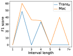
(a) CADEC

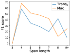
(b) CADEC

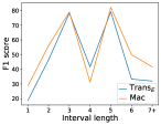
(c) ShARe 13

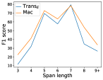
(d) ShARe 13

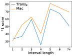
(e) ShARe 14

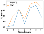
(f) ShARe 14

Intervals between segments usually make the total length of a discontinuous mention longer than continuous one. Considering the involved segments, the whole span is even longer. That is, different words of a discontinuous mention may be distant to each other, which makes discontinuous NER harder than the conventional NER task. To further evaluate the robustness of Mac in different settings, we analyze the results of test sets on different interval and span lengths. The interval length refers to the number of words between discontinuous segments. The span length refers to the number of words of the whole span. For example, for the entity mention “Sever shoulder pain” in “Sever joint, shoulder and upper body pain.”, the interval length is 5, and the span length is 8. Such phenomenon requires models to have the ability of capturing the semantic dependency between distant segments.

For the convenience of analysis, we report all datasets’ distribution on interval and span length in Table 6 and 7, respectively. And Figure 8 shows the F1 scores of Trans_E and Mac on different interval and span lengths. As we can see, Mac outperforms Trans_E in most setting. Even though Mac is defeated in some cases, the sample number in those cases is too small to disprove the superiority of Mac. For example, on CADEC, Trans_E outperforms Mac when span length is 8, but the sample number in the test set is only 10.

We figure out an interesting phenomenon: Both Mac and Trans_E show poor performance when interval length is 1 and span length is 3, even though the corresponding training samples are sufficient enough (see length = 1 in Table 6 and length = 3 in Table 7). This might result from two folds: (1) Even though the training samples are sufficient, their features and context are different from the ones in the test set; (2) discontinuous mentions with interval length equal to 1 are harder cases than the others, since only one word to separate the segments makes these discontinuous mentions very similar to the continuous ones, which confuse the model to treat them as a continuous mention. We leave this problem to our future work.

4.6.3 Analysis on Running Speed

Model	CADEC	ShARe 13	ShARe 14
TransB	29.1 Sen/s	33.4 Sen/s	33.9 Sen/s
TransE	36.3 Sen/s	40.6 Sen/s	40.3 Sen/s
Mac	193.3 Sen/s	200.2 Sen/s	198.1 Sen/s

Table 8: Comparison on running speed. Sen/s refers to the number of sentences can be processed per second.

Table 8 shows the comparison of computational efficiency between the SOTA model Trans_E, Trans_B, and our proposed Mac. All of these models are implemented by Pytorch and ran on a single Tesla V100 GPU environment. As we can see, the prediction speed of Mac is around 5 times faster than Trans_E. Since the transition-based model employs a stack to store partially processed spans and a buffer to store unprocessed tokens Dai et al. (2020b), it is difficult to utilize GPU parallel computing to speed up the extraction process. In the official implementation, Trans_E is restricted to process one token at a time, which means it is seriously inefficient and difficult to deploy in real development environment. By contrast, Mac is capable of handling data in batch mode because it is a single-stage sequence labeling model in essence.

5 Conclusion

In this paper, we reformulate discontinuous NER as the task of discovering maximal cliques in a segment graph, and propose a novel Mac architecture. It decomposes the construction of segment graph as two independent 2-D grid tagging problems, and solves them jointly in one stage, addressing the exposure bias issue in previous studies. Extensive experiments on three benchmark datasets show that Mac beats the previous SOTA method by as much as 3.5 pts in F1, while being 5 times faster. Further analysis demonstrates the ability of our model in recognizing discontinuous and overlapping entity mentions. In the future, we would like to explore similar formulation in other information extraction tasks, such as event extraction and nested NER.

References

- Alsentzer et al. (2019) Emily Alsentzer, John R Murphy, Willie Boag, Wei-Hung Weng, Di Jin, Tristan Naumann, and Matthew McDermott. 2019. Publicly available clinical bert embeddings.
- Ba et al. (2016) Jimmy Lei Ba, Jamie Ryan Kiros, and Geoffrey E Hinton. 2016. Layer normalization. arXiv preprint arXiv:1607.06450.
- Berger and Lafferty (2017) Adam Berger and John Lafferty. 2017. Information retrieval as statistical translation. In Proceedings of ACM SIGIR.
- Boginski et al. (2005) Vladimir Boginski, Sergiy Butenko, and Panos M Pardalos. 2005. Statistical analysis of financial networks. Computational statistics & data analysis.
- Bron and Kerbosch (1973) Coen Bron and Joep Kerbosch. 1973. Algorithm 457: finding all cliques of an undirected graph. Communications of the ACM.
- Chiu and Nichols (2016) Jason PC Chiu and Eric Nichols. 2016. Named entity recognition with bidirectional lstm-cnns. Transactions of the Association for Computational Linguistics.
- Dai et al. (2020a) Xiang Dai, Sarvnaz Karimi, Ben Hachey, and Cecile Paris. 2020a. Cost-effective selection of pretraining data: A case study of pretraining bert on social media. In Proceedings of EMNLP: Findings.
- Dai et al. (2020b) Xiang Dai, Sarvnaz Karimi, Ben Hachey, and Cecile Paris. 2020b. An effective transition-based model for discontinuous ner. In Proceedings of ACL.
- Dai et al. (2017) Xiang Dai, Sarvnaz Karimi, and Cecile Paris. 2017. Medication and adverse event extraction from noisy text. In Proceedings of the Australasian Language Technology Association Workshop.
- Dutta and Lauri (2019) Sourav Dutta and Juho Lauri. 2019. Finding a maximum clique in dense graphs via 2 statistics. In Proceedings of CIKM.
- Gridach (2017) Mourad Gridach. 2017. Character-level neural network for biomedical named entity recognition. Journal of biomedical informatics.
- Gui et al. (2019) Tao Gui, Ruotian Ma, Qi Zhang, Lujun Zhao, Yu-Gang Jiang, and Xuanjing Huang. 2019. Cnn-based chinese ner with lexicon rethinking. In Proceedings of IJCAI.
- Hochreiter and Schmidhuber (1997) Sepp Hochreiter and Jürgen Schmidhuber. 1997. Long short-term memory. Neural computation.
- Huang et al. (2015) Zhiheng Huang, Wei Xu, and Kai Yu. 2015. Bidirectional lstm-crf models for sequence tagging. arXiv preprint arXiv:1508.01991.
- Imbiriba et al. (2017) Tales Imbiriba, José Carlos Moreira Bermudez, and Cedric Richard. 2017. Band selection for nonlinear unmixing of hyperspectral images as a maximal clique problem. IEEE Transactions on Image Processing.
- Karimi et al. (2015) Sarvnaz Karimi, Alejandro Metke-Jimenez, Madonna Kemp, and Chen Wang. 2015. Cadec: A corpus of adverse drug event annotations. Journal of biomedical informatics.
- Khalid et al. (2008) Mahboob Alam Khalid, Valentin Jijkoun, and Maarten De Rijke. 2008. The impact of named entity normalization on information retrieval for question answering. In Proceedings of ECIR.
- Kingma and Ba (2014) Diederik P Kingma and Jimmy Ba. 2014. Adam: A method for stochastic optimization. arXiv preprint arXiv:1412.6980.
- Metke-Jimenez and Karimi (2016) Alejandro Metke-Jimenez and Sarvnaz Karimi. 2016. Concept identification and normalisation for adverse drug event discovery in medical forums. In Proceedings of ISWC.
- Mowery et al. (2014) Danielle L Mowery, Sumithra Velupillai, Brett R South, Lee Christensen, David Martinez, Liadh Kelly, Lorraine Goeuriot, Noemie Elhadad, Sameer Pradhan, Guergana Savova, et al. 2014. Task 2: Share/clef ehealth evaluation lab 2014. In Proceedings of CLEF.
- Muis and Lu (2016) Aldrian Obaja Muis and Wei Lu. 2016. Learning to recognize discontiguous entities. In Proceedings of EMNLP.
- Pradhan et al. (2015) Sameer Pradhan, Noémie Elhadad, Brett R South, David Martinez, Lee Christensen, Amy Vogel, Hanna Suominen, Wendy W Chapman, and Guergana Savova. 2015. Evaluating the state of the art in disorder recognition and normalization of the clinical narrative. Journal of the American Medical Informatics Association.
- Pradhan et al. (2013) Sameer Pradhan, Noemie Elhadad, Brett R South, David Martinez, Lee M Christensen, Amy Vogel, Hanna Suominen, Wendy W Chapman, and Guergana K Savova. 2013. Task 1: Share/clef ehealth evaluation lab 2013. In Proceedings of CLEF.
- Stix (2004) Volker Stix. 2004. Finding all maximal cliques in dynamic graphs. Computational Optimization and applications.
- Su (2019) Jianlin Su. 2019. Conditional text generation based on conditional layer normalization.
- Tang et al. (2013) Buzhou Tang, Hongxin Cao, Yonghui Wu, Min Jiang, and Hua Xu. 2013. Recognizing clinical entities in hospital discharge summaries using structural support vector machines with word representation features. In BMC medical informatics and decision making. Springer.
- Tang et al. (2018) Buzhou Tang, Jianglu Hu, Xiaolong Wang, and Qingcai Chen. 2018. Recognizing continuous and discontinuous adverse drug reaction mentions from social media using lstm-crf. Wireless Communications and Mobile Computing.
- Wang and Lu (2019) Bailin Wang and Wei Lu. 2019. Combining spans into entities: A neural two-stage approach for recognizing discontiguous entities. In Proceedings of EMNLP.
- Wang et al. (2020) Yucheng Wang, Bowen Yu, Yueyang Zhang, Tingwen Liu, Hongsong Zhu, and Limin Sun. 2020. Tplinker: Single-stage joint extraction of entities and relations through token pair linking. In Proceedings of COLING.
- Xue et al. (2020) Mengge Xue, Bowen Yu, Zhenyu Zhang, Tingwen Liu, Yue Zhang, and Bin Wang. 2020. Coarse-to-fine pre-training for named entity recognition. In Proceedings of EMNLP.
- Yu et al. (2019) Bowen Yu, Zhenyu Zhang, Tingwen Liu, Bin Wang, Sujian Li, and Quangang Li. 2019. Beyond word attention: Using segment attention in neural relation extraction. In Proceedings of IJCAI.
- Yu et al. (2021) Bowen Yu, Zhenyu Zhang, Jiawei Sheng, Tingwen Liu, Yubin Wang, Yucheng Wang, and Bin Wang. 2021. Semi-open information extraction. In Proceedings of the Web Conference.
- Yu et al. (2020) Bowen Yu, Zhenyu Zhang, and Jianlin Su. 2020. Joint extraction of entities and relations based on a novel decomposition strategy. In Proceedings of ECAI.
- Zhang et al. (2019) Wen Zhang, Yang Feng, Fandong Meng, Di You, and Qun Liu. 2019. Bridging the gap between training and inference for neural machine translation. In Proceedings of ACL.
- Zhang and Yang (2018) Yue Zhang and Jie Yang. 2018. Chinese ner using lattice lstm. In Proceedings of ACL.