Abstract

Originally conceived as a gedankenexperiment, an apparatus consisting of two Stern–Gerlach apparatuses joined in an inverted manner touched on the fundamental question of the reversibility of evolution in quantum mechanics. Theoretical analysis showed that uniting the two partial beams requires an extreme level of experimental control, making the proposal in its original form unrealizable in practice. In this work we revisit the above question in a numerical study concerning the possibility of partial-beam recombination in a spin-coherent manner. Using the Suzuki–Trotter numerical method of wave propagation and a configurable, approximation-free magnetic field, a simulation of a transversal Stern–Gerlach interferometer under ideal conditions is performed. The result confirms what has long been hinted at by theoretical analyses: the transversal Stern–Gerlach interferometer quantum dynamics is fundamentally irreversible even when perfect control of the associated magnetic fields and beams is assumed.

https://doi.org/ Quantum Dynamical Simulation of a Transversal Stern–Gerlach Interferometer Mikołaj M. Paraniak^1, and Berthold-Georg Englert^1,2,3 02.60.Lj, 03.65.-w, 03.75.Dg, 07.60.Ly, 37.25.+k
Posted on the arXiv on 31 May 2021.

1 Introduction

The experiment by Stern and Gerlach performed in 1921 (a centennial this year) Stern (1921); Gerlach and Stern (1922) proved to be of fundamental importance for the development of quantum mechanics. Far from being a thing of the past, the original design of the Stern–Gerlach apparatus (SGA) has continued to inspire new questions Bloom and Erdman (1962); Franca et al. (1992); Gorceix et al. (1994); de Oliveira and Caldeira (2006); McGregor et al. (2011); Hatifi and Durt (2020); Impens and Guéry-Odelin (2017); Mathevet et al. (2001); Xu and Xiao-Ji (2010); de Carvalho et al. (2015), and experimental techniques Robert et al. (1995); Rubin et al. (2004); Perales et al. (2007); Amit et al. (2019); Margalit et al. (2018). Professor David Bohm in his well-known textbook on quantum theory discusses a device consisting of two SGAs (see fig. 1) joined in an inverted manner so that

If the uniform magnetic fields (…) are set up in exactly the right way, and if the second inhomogeneous field is an exact duplicate of the first one, the two wave packets can be brought together into a single coherent packet. Although the precision required to achieve this result would be fantastic, it is, in principle, attainable.
—Section 22.11 in Bohm (1951)

The analysis of this possibility gave rise to what is known as the Humpty-Dumpty problem Englert et al. (1988); Schwinger et al. (1988, 1989) of coherent recombination of spatially separated partial atomic beams (i.e. the spin-up and spin-down components of the spinor wave function) coming out of an SGA, as well as to a plethora of experimental techniques within the domain of matter-wave interferometry, all of which use different approaches to work around the fantastic precision required to realize the original proposal by Bohm. Recent advances in atomic chip manufacturing allow the experimenters to realize a Stern–Gerlach-inspired interferometer Miniatura et al. (1991, 1992); Baudon et al. (1999); Machluf et al. (2013); Amit et al. (2019), whereas the accuracy required for realizing a transversal Stern–Gerlach interferometer (SGI) as originally imagined remains fantastic.

Figure 1: A side view of a transversal Stern–Gerlach interferometer as envisioned by Bohm (with the modification noted in footnote 1). Four Stern–Gerlach magnets are used to generate a magnetic field $\vec{B}$ that first splits and then recombines the atomic beam of silver atoms, which are moving with velocity $v_{y}$ through the apparatus. The spin quantization axis is determined by the homogenous field $\vec{B}_{0}$ oriented along the Z axis.

In this work we revisit the question of time-reversibility of a transversal SGI. Past theoretical work focused on the impossibility of perfect control of magnetic fields and beams, indicating a quick loss of spin coherence if such control could not be maintained Englert et al. (1988); Schwinger et al. (1988). Yet, what was also suggested by these analyses is that the very dynamics of a beam-splitting Stern–Gerlach apparatus might not be reversible as imagined, even when perfect control over involved magnetic fields and beams is assumed Englert (1997). To fill in the missing piece in the quantum Humpty-Dumpty riddle, we have performed an accurate three-dimensional wave-propagation simulation of a transversal SGI in order to capture accurately all quantum mechanical effects that arise once a full, ideal magnetic field is accounted for. The results of our simulation confirm the intuition that the quantum dynamics of a Stern–Gerlach apparatus is not reversed by the application of inverse magnetic fields, even if one has perfect control over the experimental apparatus.

2 Modeling the Transversal SGI

A beam of silver atoms prepared in a pure spin state directed along the X axis, $\ket{\psi}=\psi(x,y,z)(\ket{\uparrow}+\ket{\downarrow})/\sqrt{2}$, with the initial wave function $\psi(x,y,z)$ chosen to be a gaussian wave packet of width $\delta$,

$$\psi(x,y,z)=\frac{1}{\pi^{3/4}\delta^{3/2}}\exp(\mathrm{i}ky)\exp\Bigl(-\bigl{(}x^{2}+(y-y_{0})^{2}+z^{2}\bigr{)}/\bigl{(}2\delta^{2}\bigr{)}\Bigr{missing}),$$ (1)

$$v_{y}=\frac{\hbar k}{m}.$$

The atoms enter the apparatus from the left at time $t=0$, at $x=0$, $y=y_{0}=-L/2$, $z=0$, travel in the Y direction with velocity $v_{y}$, and exit at $y=L/2$, with $y=\pm L/2$ sufficiently far from the SGI center at $x=y=z=0$ to be outside the magnetic fringing fields. Inside the apparatus, the magnetic field $\vec{B}$ is generated by two symmetrically placed linear “magnetic charge” distributions of opposite charge at the height $a$ from the beam’s initial position, according to the arrangement depicted in fig. 2. The resulting magnetic field is symmetric across the XY plane and the nonlinear dependence on the $z$ coordinate of the magnetic field due to a single charge line, which ordinarily would result in slightly different trajectories for the spin-up and spin-down components, no longer poses an obstacle for spatial beam recombination. Furthermore, to fix the spin quantization axis along the Z axis, a bias field $\vec{B}_{0}=B_{0}\vec{e}_{z}$ in the Z direction (here $\vec{e}_{z}$ is the unit vector in the Z direction, and $B_{0}$ is the magnitude of the bias field) is applied throughout the apparatus. The magnitude of this field is chosen to be much greater than the magnitudes of the $B_{x}$, $B_{y}$ components in the apparatus to suppress the effects of Larmor precession around axes other than Z.

Figure 2: Magnetic field model used in our simulation. In the Y,Z plane we have a fictitious magnetic line charge $\lambda(y)$ at $z=-a$ and the opposite charge $-\lambda(y)$ at $z=a$. For points on the Y axis, the resulting magnetic field is in the Z direction, $\vec{B}=b_{0}(y)\vec{e}_{z}$. The model is defined by specifying $b_{0}(y)$; see section 2.2.

The Larmor spin precession angle that the particle accumulates as it travels through the apparatus results in the final spin of the atom not necessarily pointing in the X direction despite our best efforts, even if the beams are recombined coherently. It is therefore inappropriate to check whether the final spin state is equal to the initial one. Instead we measure the degree of preserved coherence, $C(t)$, by the purity of the statistical operator $M(t)$ for the spin degree of freedom,

$$M(t) =\frac{1}{2}\left(1+\left\langle{\vec{\boldsymbol{\sigma}}}\right\rangle_{\psi(t)}\cdot\vec{\boldsymbol{\sigma}}\right),$$ (2)

$$C(t) =2\,\mathrm{tr}\left(MM^{\dagger}\right)-1=\left\langle{\vec{\boldsymbol{\sigma}}}\right\rangle^{2},$$

where $\vec{\boldsymbol{\sigma}}$ is the vector of Pauli spin matrices. The spin coherence $C(t)$ ranges between $0.0$ and $1.0$, between a completely mixed spin state (coherence lost) and a pure spin state (coherence preserved), with intermediate values indicating some degree of coherence loss. After time $T$, when the particle has traversed the length of the apparatus $L$ and reached the position $y=L/2$, it emerges at the right and its spin coherence is measured. It is our goal that the final value $C(T)$ of the spin coherence is as close to its maximal value $1.0$ as possible; in a perfect experiment we shall have $C(T)=1.0$.

During the evolution the peak separation between the partial beams reaches $\Delta Z(T/2)$ (henceforth denoted by $\Delta Z$). One has to ensure that $\Delta Z$ is large compared with the width $\delta$ of the atom wave packet to say that the partial beams have truly separated. If despite partial beam separation in the middle of the apparatus the spin coherence has been preserved, then the evolution in the left half of the apparatus has been reversed, or in the playful language of Englert et al. (1988), Humpty-Dumpty, which is really an egg, has been put back again after his great fall. After this overview of the experiment we move on to describing the methods used in the simulation.

2.1 Quantum Dynamics of the Apparatus

Following the usual quantum treatment of an SGA, we have the following Hamiltonian describing the spin-1/2 silver atom comprising the beam:

$$\mathcal{H}=\frac{\vec{\boldsymbol{P}}^{2}}{2m}-\mu\vec{\boldsymbol{\sigma}}\cdot\vec{B}(\vec{\boldsymbol{R}})$$ (3)

with the momentum operator $\vec{\boldsymbol{P}}=(\boldsymbol{P}_{x},\boldsymbol{P}_{y},\boldsymbol{P}_{z})$, the position operator $\vec{\boldsymbol{R}}=(\boldsymbol{R}_{x},\boldsymbol{R}_{y},\boldsymbol{R}_{z})$, the magnetic moment $\mu$, the vector of Pauli spin matrices $\vec{\boldsymbol{\sigma}}=(\boldsymbol{\sigma}_{x},\boldsymbol{\sigma}_{y},\boldsymbol{\sigma}_{z})$, and the position-dependent magnetic field $\vec{B}(\vec{\boldsymbol{R}})$ in the apparatus. The numerical values for $m$ and $\mu$ that are used in the simulation, and other simulation parameters are included in the appendix.

To solve the equations of motion with an accuracy high enough to model coherent beam recombination we employ a fourth-order Suzuki–Trotter operator splitting method Suzuki (1976). In this scheme, given any Hamiltonian with a potential-energy term $V(\vec{\boldsymbol{R}})$, the time propagator $U=e^{-\mathrm{i}t/\hbar\,(\vec{\boldsymbol{P}}^{2}/(2m)+V(\vec{\boldsymbol{R}}))}$, which advances the wave function by a time step $t$, is split into several exponential terms, each involving only the momentum operator or the potential operator with coefficients specially chosen, such that the whole formula is accurate to a certain order $k$,

$$U_{N}=\prod^{\left\lceil N/2\right\rceil}_{i=1}\mathrm{e}^{-\frac{\mathrm{i}t}{\hbar}\alpha_{i}V(\vec{\boldsymbol{R}})}\mathrm{e}^{-\frac{\mathrm{i}t}{\hbar}\beta_{i}\frac{\vec{\boldsymbol{P}}^{2}}{2m}}=\mathrm{e}^{-tA_{1}}\mathrm{e}^{-tB_{1}}\mathrm{e}^{-tA_{2}}\mathrm{e}^{-tB_{2}}\cdots,$$ (4)

where $A_{i}$, $B_{i}$ correspond respectively to potential and momentum operator terms. While approximations $U_{N}$ for increasing $N$ yield higher-order formulas and can in principle achieve any desired level of accuracy, the computational cost goes up considerably with increasing $N$, as between each application of operators either in momentum or in position space one has to perform a Fourier transformation on the wave function. For our purpose we have chosen a fourth-order Suzuki–Trotter method of a special form that involves a gradient term of the potential and five operator terms in total, compared with 11 terms in the standard Suzuki–Trotter formula needed to achieve the same order Hatano and Suzuki (2005); Chin (1997); Hue et al. (2020). The time propagator in this “$7\star$ approximation” is

$$\begin{split}U_{7\star}=&\exp(-\frac{\mathrm{i}t}{6\hbar}V(\vec{\boldsymbol{R}}))\exp(-\frac{\mathrm{i}t}{4\hbar m}\vec{\boldsymbol{P}}^{2})\\ &\times\exp(-\frac{\mathrm{i}t}{\hbar}\left(\frac{2}{3}V(\vec{\boldsymbol{R}})-\frac{1}{72m}\left[t\gradient{V}(\vec{\boldsymbol{R}})\right]^{2}\right))\\ &\times\exp(-\frac{\mathrm{i}t}{4\hbar m}\vec{\boldsymbol{P}}^{2})\exp(-\frac{\mathrm{i}t}{6\hbar}V(\vec{\boldsymbol{R}})),\end{split}$$ (5)

and to propagate the wave function the above five unitary operators are applied in their respective space. For instance, the application of the first two terms from the right

$$\exp(-\frac{\mathrm{i}t}{4\hbar m}\vec{\boldsymbol{P}}^{2})\exp(-\frac{\mathrm{i}t}{6\hbar}V(\vec{\boldsymbol{R}}))$$

on $\psi(\vec{R},t_{0})$ as part of the algorithm requires two Fourier transformations $\mathcal{F}$,

$$\psi(\vec{R},t_{0}+t)=\cdots\mathcal{F}^{-1}\left\{\exp(-\frac{\mathrm{i}t}{4\hbar m}\vec{\boldsymbol{P}}^{2})\mathcal{F}\left\{\exp(-\frac{\mathrm{i}t}{6\hbar}V(\vec{\boldsymbol{R}}))\psi(\vec{R},t_{0})\right\}\right\}.$$ (6)

A single application of the $U_{7\star}$ propagator requires the execution of four Fourier transformations for a spinless wave function. Time propagation of a spin-1/2 particle will require eight Fourier transformations per time step, an operation that contributes heavily to the computational cost.

Once this split-operator machinery is in place we can simulate the quantum evolution of any system described by a reasonable Hamiltonian with a position-dependent potential, including the quantum dynamics of an SGI. However, when attempting to do so according to the method presented above, one is quickly faced with rising computational space and time resources required to perform the computation to a sufficient degree of accuracy. The storage cost of a wave function across the region of the apparatus is prohibitive, as is the time required to perform repeated Fourier transformations in each time step.

To make the calculation feasible, we transform the Hamiltonian into the co-moving frame of the atomic beam traveling with velocity $v_{y}$ along the Y axis of the apparatus. This is done at the cost of making the potential term in the Hamiltonian time-dependent,

$$\mathcal{H}=\frac{\vec{\boldsymbol{P}}^{2}}{2m}-\mu\vec{\boldsymbol{\sigma}}\cdot\vec{B}(\boldsymbol{X},y_{0}+v_{y}\,t-\boldsymbol{Y},\boldsymbol{Z}),$$ (7)

and thus requires a re-evaluation of the split-operator method which, presented in its most basic form, is applicable only to Hamiltonians not explicitly dependent on time. The extension of the split-operator method to time-dependent non-commuting Hamiltonians is treated in full generality in Suzuki (1993). Here we just note the elegant result: in the time-dependent split-operator method $U_{7\star T}$ the reference time has to be advanced cumulatively at each encountered $\exp(-\frac{\mathrm{i}t\beta}{\hbar}\frac{\vec{\boldsymbol{P}}^{2}}{2m})$ term, $T^{\prime}=T+\beta\,t$, so that subsequently applied potential operator terms use the newly advanced time $T^{\prime}$, until the next application of a position propagator and so on. The resulting formula for the time-dependent propagator is then guaranteed to be accurate to the same order as the original formula. Using this simple prescription we readily obtain the time-dependent propagator $U_{7\star T}$, for the evolution from time $T$ to time $T+t$,

$$\begin{split}U_{7\star T}=&\exp(-\frac{\mathrm{i}t}{6\hbar}V(\vec{\boldsymbol{R}},T+t))\exp(-\frac{\mathrm{i}t}{4\hbar m}\vec{\boldsymbol{P}}^{2})\\ &\times\exp(-\frac{\mathrm{i}t}{\hbar}\left(\frac{2}{3}V(\vec{\boldsymbol{R}},T+t/2)-\frac{t^{2}}{72m}\left[\gradient{V}(\vec{\boldsymbol{R}},T+t/2)\right]^{2}\right))\\ &\times\exp(-\frac{\mathrm{i}t}{4\hbar m}\vec{\boldsymbol{P}}^{2})\exp(-\frac{\mathrm{i}t}{6\hbar}V(\vec{\boldsymbol{R}},T)).\end{split}$$ (8)

In this way one has to keep track only of the wave function in the region required to model the beam deflection in the Z axis, which is very small compared with the total extent of the apparatus, as the movement along the Y direction has been taken care of by transforming the Hamiltonian into the co-moving frame. The outstanding challenge is an efficient and accurate computation of the magnetic field $\vec{B}(x,y,z)$, which in each time step has to be evaluated across the domain of the wave function, now in the co-moving frame of the beam.

2.2 Magnetic Field in the Apparatus

To our best knowledge all previous quantum treatments of Stern–Gerlach-like experiments employed a magnetic field that either did not satisfy the Maxwell equations through the neglect of the X and Y field components and linear approximations Englert et al. (1988); Schwinger et al. (1988); Japha (2019), or used a simple model of a magnetic field that neglects the fringing fields at the entrance and exit of the apparatus Manoukian and Rotjanakusol (2003); Hsu et al. (2011). For the purpose of our work it is crucial that the employed field model is free from both of these approximations, since it is clear that either of these simplifications will result in an apparatus that will seemingly have no problem with reuniting the partial beams in a coherent manner, as long as the beams and fields are accurately controlled.

In the traditional design, at least four Stern–Gerlach magnets have to be employed. As the particle goes through the apparatus, the partial beams corresponding to the spin-up and spin-down components are first imparted a momentum which leads to their spatial separations as seen in the schematic trajectories in fig. 1. Subsequently, the evolution both in momentum and position has to be reversed. The second and third magnets first decelerate the particle and then impart momentum equal in magnitude to the momentum gained in the first stage, and finally the last magnet decelerates the particle, whereupon, if the conditions were ideal, we should find the partial beams reunited, and the particle in a pure spin state.

In our scheme, we exploit the correspondence between the Maxwell equations for the electric field and the static magnetic field,

$$\curl\vec{E}=0,\quad \divergence\vec{E}=0,$$ (9)

$$\curl\vec{B}=0,\quad \divergence\vec{B}=0,$$

and introduce a fictitious magnetic “charge” potential $\phi$, which obeys the Laplace equation

$$\gradient^{2}\phi=0,$$ (10)

and results in a physical magnetic field

$$\vec{B}=-\gradient{\phi},$$ (11)

in full analogy to a static electric field. In this manner we obtain a configurable model of a magnetic field free from approximations. This is in contrast to other approaches to the Humpty-Dumpty problem, which tend to turn the problem of reversing the evolution into a technical difficulty depending solely upon the experimenter’s skill, thereby possibly concealing difficulties of a more fundamental nature, while our aim is precisely to uncover those difficulties that arise once all simplifications are put aside.

The scalar potential for the pair of magnetic line charges (see fig. 2) is

$$\phi(\vec{r}) =\int_{-\infty}^{\infty}\mathrm{d}y^{\prime}\,\lambda(y^{\prime})\Bigl{(}\bigl{[}(y-y^{\prime})^{2}+s_{+}^{2}\bigr{]}^{-1/2}-\bigl{[}(y-y^{\prime})^{2}+s_{-}^{2}\bigr{]}^{-1/2}\Bigr{)}$$

$$=\int_{-\infty}^{\infty}\frac{\mathrm{d}k}{\pi}\,\mathrm{e}^{-\mathrm{i}ky}\bigl{[}K_{0}\bigl{(}|k|s_{+}\bigr{)}-K_{0}\bigl{(}|k|s_{-}\bigr{)}\bigr{]}\int_{-\infty}^{\infty}\mathrm{d}y^{\prime}\,\mathrm{e}^{\mathrm{i}ky^{\prime}}\lambda(y^{\prime})\,,$$ (12)

where

$$s_{\pm}=\sqrt{x^{2}+(z\pm a)^{2}}$$ (13)

are the respective distances from the charged lines, and $K_{0}(\ )$ is the zeroth-order modified Bessel function of the second kind. On the Y axis, we have

$$-\gradient\phi\Bigr{|}_{x=z=0}=-\frac{\partial\phi}{\partial z}\Bigr{|}_{s_{\pm}=a}\vec{e}_{z}=2b_{0}(y)\vec{e}_{z}$$ (14)

with $b_{0}(y)$ and $\lambda(y)$ related to each other by

$$\int_{-\infty}^{\infty}\mathrm{d}y\,\mathrm{e}^{\mathrm{i}ky}\lambda(y)=\frac{1}{2|k|\,K_{1}\bigl{(}|k|a\bigr{)}}\int_{-\infty}^{\infty}\mathrm{d}y\,\mathrm{e}^{\mathrm{i}ky}b_{0}(y)\,,$$ (15)

where $K_{1}(\ )$ is the first-order modified Bessel function of the second kind. Upon expressing $\phi(\vec{r})$ in terms of $b_{0}(y)$,

$$\phi(\vec{r})=\int_{-\infty}^{\infty}\frac{\mathrm{d}k}{2\pi}\,\mathrm{e}^{-\mathrm{i}ky}\frac{K_{0}\bigl{(}|k|s_{+}\bigr{)}-K_{0}\bigl{(}|k|s_{-}\bigr{)}}{|k|\,K_{1}\bigl{(}|k|a\bigr{)}}\int_{-\infty}^{\infty}\mathrm{d}y^{\prime}\,\mathrm{e}^{\mathrm{i}ky^{\prime}}b_{0}(y^{\prime})\,,$$ (16)

one confirms that $\phi(\vec{r})$ satisfies the Laplace equation (10) for $s_{\pm}>0$ by an exercise in differentiation, for which the relations Ambramowitz and Stegun (1964)

$$K^{\prime}_{0}(z)=-K_{1}(z),\qquad K^{\prime}_{1}(z)=-\frac{1}{z}K_{1}(z)-K_{0}(z)$$ (17)

are useful.

After including the bias field $B_{0}\vec{e}_{z}$ and a strength parameter $f$, the magnetic field is

$$\vec{B}=(-\gradient{\phi}+B_{0}\vec{e}_{z})\,f.$$ (18)

Rather than specifying the line-charge density $\lambda(y)$, we define the model by the choice for $b_{0}(y)$, essentially $\vec{B}=B_{z}\vec{e}_{z}$ along the level trajectory of the atom that traverses the SGI. This makes it easier to ensure that the magnetic field decreases rapidly outside the SGA. Indeed, as we show below, one can model a magnetic field suitable for coherent beam recombination by an appropriate choice for $b_{0}(y)$, the strength parameter $f$, and the separation ${d=2a}$ between the two line charges.

2.3 Beam Recombination in the Calibrated Magnetic Field

The conventional treatment of an SGA assumes that the atom’s deflection is caused by a linear $B_{z}\propto z$ field, thus making the force $F_{z}\propto\frac{\partial B_{z}}{\partial z}$ position independent, which greatly aids in subsequent beam recombination. However, a field like this is unphysical, it does not satisfy the Maxwell equations, and thus conclusions regarding the reversibility of the SGA’s dynamics based on reasoning which neglects this issue are unconvincing as they risk missing quantum effects that might have an impact on the spin coherence. A physical field will necessarily have a non-linear dependence on the $z$ coordinate and thus requires fine tuning to make the partial beams come back to zero separation.

In our scheme one can calibrate the field to result in a desired peak separation $\Delta Z$ by adjusting the field strength parameter $f$ and the distance $2a$ between the top and bottom line charges. For $b_{0}(y)$ we choose a magnetic field profile composed of two gaussians with an adjustable width parameterized by $\alpha$ (as shown schematically in fig. 2),

$$b_{0}(y)=\frac{\alpha}{\sqrt{2\pi}}\biggl{[}\exp\Bigl(-(\alpha y)^{2}/2\Bigr{missing})-\sqrt{2}\exp\Bigl(-(\alpha y)^{2}\Bigr{missing})\biggr{]}$$ (19)

The parameter $\alpha$ determines the longitudinal stretch of the apparatus over which the particle is deflected, influencing the overall deflection, as well as the range of the fringing fields — the wider the gaussian peaks, the slower the decay of the magnetic field off the Y axis. As such, a judicious choice of $\alpha$ is needed, firstly to avoid a gaussian that is too narrow and expensive to resolve numerically, and secondly to avoid a gaussian too wide, which then makes it necessary to model an apparatus sufficiently wide to have the fringing fields negligible at both ends of the apparatus.

The force in the Z direction resulting from such a profile, as shown in fig. 3, effectively consists of four regions of unequal length symmetric accross the Z axis. These regions are indicated by the direction of the force in each sector: $+$, $-$, $-$, $+$. Such an arrangement allows us to mimic the effect of the four-magnet setup of fig. 1 in a simple way, without having to introduce a model of the magnetic field for each SG magnet separately. Note that this $b_{0}(y)$ is even in $y$ and, therefore, we can replace the exponential factors in eq. (16) by their real parts.

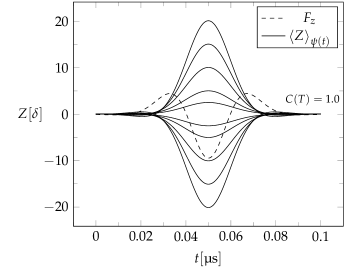
Figure 3: Trajectories of the partial beams for beam separations $\Delta Z=5,10,20,30,40[\delta]$, according to the quantum dynamics of the simplified Hamiltonian. The spin-up and spin-down partial trajectories for each peak separation $\Delta Z$ are symmetric. The final coherence is rounded to four decimal places and is $C(T)=1.0$ regardless of the magnitude of peak separation. The slightly visible ribbon shape of the trajectories near the input and output of the apparatus for higher peak separations is a feature of the fringing fields of the employed magnetic field. The dashed line is the force $F_{z}$, in units of $\mu\,b_{0}(y=0)/a$, acting on the partial spin-up beam of the largest separation $\Delta Z=40\delta$.

The field felt by the particle along its trajectory is approximately $B_{z}\approx b_{0}(y)$, as long as the deflections are much smaller than the length scale of the field changes. Then, the vanishing of the integral

$$\int^{\infty}_{-\infty}\mathrm{d}y\,b_{0}(y)=0$$ (20)

makes the Larmor precession around the Z axis approximately equal to 0, with the spin pointing in the X direction at the output. Beam recombination along the Y axis is facilitated by energy conservation — changes in potential energy coming chiefly from the changes in $B_{z}\approx b_{0}(y)$ along the trajectory in the left half of the interferometer (fig. 1) are reversed by the opposite changes in the right half (since $b_{0}(-y)=b_{0}(y)$). However, the choice $b_{0}(y)$ dictated by this reasoning is not a sufficient guarantee of coherent recombination. The real trajectory is not level and becomes minutely sensitive to the exact field, non-linear in its $z$ coordinate dependence, in the apparatus. With the two remaining parameters at hand, the line charge separation $2a$ and the field strength $f$, we perform a bisection search for these parameters, constrained by the desired value of the peak separation $\Delta Z(T/2)\equiv\Delta Z$ and with the objective of vanishing final spatial separation of the beams,

$$\Delta Z(T)\leq 10^{-6}\delta.$$ (21)

This is done in a semiclassical manner: the Z axis quantum and classical dynamics are in good agreement, the classical simulation being much cheaper to perform than the quantum counterpart, thus making this optimization scheme feasible. We obtain a range of parameters $a$, $f$ that result in spin-coherent recombination for different values of the for peak separation, $\Delta Z=1\delta,2\delta,\dots,40\delta$. With this set of optimized parameters $\{a,f\}$ at hand (their values can be found in the appendix), each choice resulting in a suitable magnetic field and trajectories with peak separation $\Delta Z_{a,f}$, we can now proceed to simulating the quantum dynamics of the SGI.

3 Quantum Dynamical Simulation of the SGI

Using the optimized magnetic fields and the methods discussed in the preceding sections, we can now perform the wave-propagation simulation of the SGI. In the first step, we performed a quantum simulation of the beam’s evolution in the optimized fields neglecting the microscopic quantum motions in the X, Y axes. The effective Hamiltonian for this case is a simplified one-dimensional version of the full Hamiltonian of eq. (7):

$$\mathcal{H}=\frac{\boldsymbol{P}_{z}^{2}}{2m}-\mu\boldsymbol{\sigma_{z}}B_{z}(0,y_{0}+v_{y}\,t,\boldsymbol{Z}).$$ (22)

The simulated beam trajectories are presented in fig. 3.

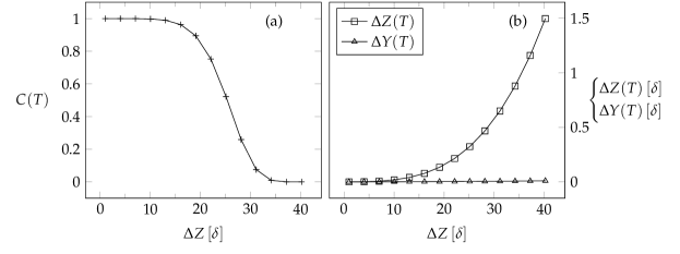
Figure 4: The final spin coherence $C(T)$ in panel (a) and relative partial beam displacements $\Delta Z(T)$, $\Delta Y(T)$ in panel (b) as a function of increasing peak separation $\Delta Z$. The magnetic field that results in perfect beam recombination when the microscopic quantum movements in the X and Y axis are neglected, is no longer sufficient to reverse the full quantum evolution when $\Delta Z$ becomes appreciable.

Regardless of the magnitude of the peak separation $\Delta Z=1\delta,2\delta,\dots,40\delta$ the beams are recombined coherently. Note that this happens only because the magnetic field, which depends on the $z$ coordinate in a non-linear fashion (making the force $F_{z}$ position dependent), is finely calibrated for each $\Delta Z$ separately. The standard recipe of taking the “reverse” fields to reverse the evolution of the beam that underwent the splitting by SG magnets, therefore seems to work, as long as the fields are calibrated in an “exactly right” way. But is it really true? The standard argument assumes that the neglected X and Y movements are miniscule compared with the large deflection in the Z axis and, therefore, should not influence the overall analysis. However, since coherent beam recombination is concerned precisely with the relative microscopic realignment of the partial spin-up, spin-down beams, it is necessary to simulate the full dynamics.

We calculated the quantum dynamics of the original Hamiltonian of eq. (7), again varying the peak separation $\Delta Z$ and measuring the final spin coherence $C(T)$. The peak separation-spin coherence curve, together with the final relative displacements of the partial beams in $y$, $z$ coordinates are presented in fig. 4. Although for very small separations up to $\Delta Z=10\delta$ the partial beams are recombined coherently—note that this does not mean that the evolution was fully reversed: the spreading of the wave packet, though inconsequential, has not been undone—once the peak separation exceeds this value, the evolution rapidly becomes irreversible, with $C(T)=0.0$ indicating complete spin decoherence by the time separation reaches $\Delta Z=35\delta$. The cause of this loss of spin coherence is the growing microscopic separation in the Z and Y axes between the up and down spin components as shown in fig. 4b, which, although barely exceeding $\delta$ in Z and negligible in Y, is enough to completely prevent coherent beam recombination.

4 Discussion and Conclusion

An SGA entangles the spin degree of freedom of a spin-1/2 atom with its orbital degrees of freedom, so that the outcome of a position measurement informs us about the spin of the atom (“up” or “down” in the traverse direction that is probed). The transition from the initial not-entangled state to the final entangled state is unitary; it is not an irreversible event that can be amplified and recorded. Since unitary processes compose a group, they are invertible in a mathematical sense. Is the entangling action of a SGA also invertible as a physical process — by another unitary transition, that is?

“Yes,” answered Bohm Bohm (1951) and later Wigner Wigner:AJP63 , and others parroted their wisdom. While Bohm acknowledged that the reversal would require a “fantastic” precision in controlling the apparatus and Wigner observed that such an experiment “would be difficult to perform,” both took the reversibility for granted and did not elaborate on the matter. It is, however, unclear whether elementary unitary quantum processes are reversible — in marked contrast to macroscopic processes, which are known to be irreversible, as witnessed by the folk wisdom of the medieval Humpty-Dumpty rhyme, the laws of thermodynamics, the lessons of deterministic chaos, the ubiquitous ageing of living organisms, and other familiar phenomena.

In the particular situation of an SGA, the atom’s spin and orbital degrees of freedom are coupled by the force resulting from the magnetic field gradient, and only this coupling is available for reversing the action of the SGA in a unitary fashion. We cannot undo the action of the unitary evolution operator $\exp\bigl(-\mathrm{i}tH/\hbar\bigr{missing})$, with $H$ as in eq. (3), by applying its inverse $\exp\bigl(-\mathrm{i}t(-H)/\hbar\bigr{missing})$ because $-H$ is not a physical Hamiltonian — so much for mathematical reversibility. Rather, we must carefully tailor the magnetic field to implement the disentangling reversal as well as we can.

We recall that Bohm’s “fantastic” accuracy amounts to controlling the macroscopic devices with submicroscopic precision Englert et al. (1988), and if such control is granted, Maxwell’s equations prevent us from undoing the entanglement perfectly Schwinger et al. (1988), even if we neglect the effects of fringing fields (as is the case in Schwinger et al. (1988)). These theoretical works are here supplemented by a numerical study that fully accounts for the quantum dynamics with a magnetic field that obeys Maxwell’s equations throughout the volume probed by the atom.

Thereby we assume that there are no uncontrolled imperfections. This is, of course, an over-idealization that lacks justification (as it ignores the lesson of Englert et al. (1988)). But even with this stretch we find that the action of the SGA cannot be undone if the SGA serves its purpose, namely separates the atoms into well distinguishable partial beams — $\Delta Z>20\delta$, say.

In conclusion, the accurate wave-propagation results presented here quantitatively confirm that the microscopic quantum dynamical effects in a transversal SGI apparatus are enough to quickly destroy spin coherence beyond recovery. The deceptively simple nature of the Stern–Gerlach beam-splitting apparatus and the seemingly obvious proposal to reverse its evolution by employing “reverse” fields might lead one to assume the fundamental reversibility of its quantum evolution, as long as the apparatus is controlled sufficiently well. Such assumptions are, however, unwarranted.

Appendix: Particle properties and initial wave function

As in the original Stern–Gerlach experiment, we used a beam of silver atoms to simulate the splitting and recombination. The values of the various variables are given in table Appendix: Particle properties and initial wave function. In the lapse of time $T$, the width of the wave function would increase by a factor of

$$\sqrt{1+{\left(\frac{\hbar T}{m\delta^{2}}\right)}^{2}}\approx 1.16$$ (23)

if there were force-free motion, and this amount of spreading is of no consequence.

[b]Values used in the simulation: atom properties, apparatus geometry, and initial wave function. first variable value occurrence description $m$ $107.8682\,$\mathrm{D}\mathrm{a}$$ in eq. (LABEL:eq:psi-gaussian) mass of a silver atom ($\mathrm{D}\mathrm{a}$: dalton) $\mu$ $\frac{1}{2}\mu_{\mathrm{B}}$ in eq. (3) magnetic moment ($\mu_{\mathrm{B}}$: Bohr magneton) $L$ $25\,$\mathrm{\SIUnitSymbolMicro m}$$ after eq. (LABEL:eq:psi-gaussian) length of the SGI $T$ $0.1\,$\mathrm{\SIUnitSymbolMicro s}$$ after eq. (2) time to traverse the SGI $y_{0}=-L/2$ $-12.5\,$\mathrm{\SIUnitSymbolMicro m}$$ in eq. (LABEL:eq:psi-gaussian) initial position $v_{y}=L/T$ $250\,$\mathrm{m}\,\mathrm{s}^{-1}$$ in eq. (LABEL:eq:psi-gaussian) initial velocity $\delta$ $0.01\,$\mathrm{\SIUnitSymbolMicro m}$$ in eq. (LABEL:eq:psi-gaussian) width of the initial wave function

Appendix: Magnetic Field

The parameter $\alpha$ of the magnetic profile function $b_{0}(y)$ of eq. (19), depicted in fig. 2, was chosen to be

$$\alpha=0.3\,$\mathrm{\SIUnitSymbolMicro m}$^{-1}.$$ (24)

The example parameters of the optimized fields, rounded to five decimal places, are displayed in table Appendix: Magnetic Field. In fig. 5 the field lines of the $B_{z}$ component of the field calibrated for $\Delta Z=40\delta$ (the largest simulated peak separation) are shown. The overall magnitude of the $B_{y}$ component of the generated field is actually larger than that the magnitude of $B_{z}$. By adjusting $B_{0}$ we make sure that the resulting $B_{z}$ field component is the largest magnetic field component in the apparatus. For the fields used in the simulations the suitable value of $B_{0}$ in units of $b_{0}(y=0)$, where a.u. denotes atomic units of magnetic field strength, is

$$B_{0}=100.0\,\textrm{a.u.}\big{/}\bigl{|}b_{0}(y=0)\bigr{|}\approx 2017.$$ (25)

[t]Optimized magnetic field parameters: beam separation $\Delta Z$ (cf. fig. 3), field-strength parameter $f$ of eq. (18), and line-charge distance $a$ (cf. fig. 2). $\Delta Z[\delta]$ $f$ $a[$\mathrm{\SIUnitSymbolMicro m}$]$ 25 0.00011 0.71919 10 0.00030 0.04353 20 0.00081 1.61404 30 0.00147 2.19168 40 0.00226 2.85283

The evaluation of the magnetic field integrals, the gradient of $\phi$ of eq. (16), across the wave function domain (the grid in the simulation for highest separation $\Delta Z=40\delta$ consists of 800 million points) was too time-consuming. Since the whole simulation was performed on a distributed computing cluster; we divided the domain into subdomains, with each subdomain being simulated on a separate processor. In each subdomain, then, the magnetic field $\vec{B}$ was approximated by a second-order Taylor approximation, centered at the weighted position of the wave function chunk in a particular domain, and there was no loss of accuracy from this.

The overall computational resources spent in the simulation of $\Delta Z=40\delta$ were as follows. The simulation was run on 40 cores in parallel, with a special parallelized FFT routine as the only step requiring inter-core communication. The computation time spent per core was 15 hours, a total of 600 hours. The breakdown of the average time spent in a single step of the time evolution loop: 30% spent on performing FFTs, 39% on potential propagators (costly because of field evaluations discussed in the preceding paragraph), 28% on observables calculations, and 3% on momentum propagators. The overall memory allocation per core was 3GB, a total of 120GB.

Figure 5: Lines of constant $B_{z}$ of the magnetic field calibrated for $\Delta Z=40\delta$ shown in the YZ plane. The sign of the field in a particular region is indicated by a $+$ ($B_{z}>0$) and $-$ ($B_{z}<0$). The nested contours increase in field strength as the field gets closer to the line charges located at a distance $\pm a$ at the top and bottom, according to table Appendix: Magnetic Field. Note that the width of the gaussian wave packet $\delta$ is small compared with the overall changes of the field. In the middle of the apparatus ($Z=0$ line) the field vanishes exactly because the line charges of opposite sign are placed symmetrically across the XY plane.

References

References

- Stern (1921) Stern, O. Ein Weg zur experimentellen Prüfung der Richtungsquantelung im Magnetfeld. Zeitschrift für Physik 1921, 7, 249–253. doi:\changeurlcolorblue10.1007/BF01332793.
- Gerlach and Stern (1922) Gerlach, W.; Stern, O. Der experimentelle Nachweis des magnetischen Moments des Silberatoms. Zeitschrift für Physik 1922, 8, 110–111. doi:\changeurlcolorblue10.1007/BF01329580.
- Bloom and Erdman (1962) Bloom, M.; Erdman, K. The transverse Stern–Gerlach experiment. Canadian Journal of Physics 1962, 40, 179–193.
- Franca et al. (1992) França, H.M.; Marshall, T.W.; Santos, E.; Watson, E.J. Possible interference effect in the Stern–Gerlach phenomenon. Physical Review A 1992, 46, 2265–2270. doi:\changeurlcolorblue10.1103/PhysRevA.46.2265.
- Gorceix et al. (1994) Gorceix, O.; Robert, J.; Chormaic, S.N.; Miniatura, C.; Baudon, J. Dispersive and nondispersive phase shifts in atomic Stern–Gerlach interferometry. Physical Review A 1994, 50, 5007.
- de Oliveira and Caldeira (2006) de Oliveira, T.R.; Caldeira, A.O. Dissipative Stern–Gerlach recombination experiment. Physical Review A 2006, 73, 042502. doi:\changeurlcolorblue10.1103/PhysRevA.73.042502.
- McGregor et al. (2011) McGregor, S.; Bach, R.; Batelaan, H. Transverse quantum Stern–Gerlach magnets for electrons. New Journal of Physics 2011, 13, 065018.
- Hatifi and Durt (2020) Hatifi, M.; Durt, T. Revealing self-gravity in a Stern–Gerlach Humpty-Dumpty experiment. eprint arXiv:2006.07420 2020.
- Impens and Guéry-Odelin (2017) Impens, F.; Guéry-Odelin, D. Shortcut to adiabaticity in a Stern–Gerlach apparatus. Physical Review A 2017, 96, 043609. doi:\changeurlcolorblue10.1103/PhysRevA.96.043609.
- Mathevet et al. (2001) Mathevet, R.; Brodsky, K.; Perales, F.; Boustimi, M.; de Lesegno, B.V.; Reinhardt, J.; Robert, J.; Baudon, J. Some new effects in atom Stern–Gerlach interferometry. In Atomic and Molecular Beams; Springer, 2001; pp. 81–94.
- Xu and Xiao-Ji (2010) Xu, X.; Xiao-Ji, Z. Phase-dependent effects in Stern–Gerlach experiments. Chinese Physics Letters 2010, 27, 010309. doi:\changeurlcolorblue10.1088/0256-307X/27/1/010309.
- de Carvalho et al. (2015) de Carvalho, C.R.; Jalbert, G.; Impens, F.; Robert, J.; Medina, A.; Zappa, F.; de Castro Faria, N.V. Toward a test of angular-momentum coherence in a twin-atom interferometer. Europhysics Letters (EPL) 2015, 110, 50001.
- Robert et al. (1995) Robert, J.; Gorceix, O.; Lawson-Daku, J.; Chormaic, S.N.; Miniatura, C.; Baudon, J.; Perales, F.; Eminyan, M.; Rubin, K. Stern–Gerlach atomic interferometry with space- and time-dependent magnetic fields. Annals of the New York Academy of Sciences 1995, 755, 173–181. doi:\changeurlcolorblue10.1111/j.1749-6632.1995.tb38965.x.
- Rubin et al. (2004) Rubin, K.; Eminyan, M.; Perales, F.; Mathevet, R.; Brodsky, K.; Viaris de Lesegno, B.; Reinhardt, J.; Boustimi, M.; Baudon, J.; Karam, J.C. Atom interferometer using two Stern–Gerlach magnets. Laser Physics Letters 2004, 1, 184–193.
- Perales et al. (2007) Perales, F.; Robert, J.; Baudon, J.; Ducloy, M. Ultra thin coherent atom beam by Stern–Gerlach interferometry. Europhysics Letters (EPL) 2007, 78, 60003. doi:\changeurlcolorblue10.1209/0295-5075/78/60003.
- Amit et al. (2019) Amit, O.; Margalit, Y.; Dobkowski, O.; Zhou, Z.; Japha, Y.; Zimmermann, M.; Efremov, M.A.; Narducci, F.A.; Rasel, E.M.; Schleich, W.P. T3 Stern–Gerlach matter-wave interferometer. Physical Review Letters 2019, 123, 083601.
- Margalit et al. (2018) Margalit, Y.; Zhou, Z.; Dobkowski, O.; Japha, Y.; Rohrlich, D.; Moukouri, S.; Folman, R. Realization of a complete Stern–Gerlach interferometer. eprint arXiv:1801.02708 2018.
- Bohm (1951) Bohm, D. Quantum Theory; Prentice-Hall, 1951.
- (19) Wigner, E.P. The Problem of Measurement. American Journal of Physics 1963, 31, 6–15. doi:\changeurlcolorblue10.1119/1.1969254.
- Englert et al. (1988) Englert, B.-G.; Schwinger, J.; Scully, M.O. Is spin coherence like Humpty-Dumpty? I. Simplified treatment. Foundations of Physics 1988, 18, 1045–1056. doi:\changeurlcolorblue10.1007/BF01909939.
- Schwinger et al. (1988) Schwinger, J.; Scully, M.O.; Englert, B.-G. Is spin coherence like Humpty-Dumpty? II. General theory. Zeitschrift für Physik D Atoms, Molecules and Clusters 1988, 10, 135–144. doi:\changeurlcolorblue10.1007/BF01384847.
- Schwinger et al. (1989) Schwinger, J.; Scully, M.O.; Englert, B.-G. Spin coherence and Humpty-Dumpty. III. The effects of observation. Physical Review. A, General Physics 1989, 40, 1775–1784. doi:\changeurlcolorblue10.1103/physreva.40.1775.
- Miniatura et al. (1991) Miniatura, C.; Perales, F.; Vassilev, G.; Reinhardt, J.; Robert, J.; Baudon, J. A longitudinal Stern–Gerlach interferometer: the “beaded” atom. Journal de Physique II 1991, 1, 425–436.
- Miniatura et al. (1992) Miniatura, C.; Robert, J.; Le Boiteux, S.; Reinhardt, J.; Baudon, J. A longitudinal Stern–Gerlach atomic interferometer. Applied Physics B 1992, 54, 347–350.
- Baudon et al. (1999) Baudon, J.; Mathevet, R.; Robert, J. Atomic interferometry. Journal of Physics B: Atomic, Molecular and Optical Physics 1999, 32, R173–R195. doi:\changeurlcolorblue10.1088/0953-4075/32/15/201.
- Machluf et al. (2013) Machluf, S.; Japha, Y.; Folman, R. Coherent Stern–Gerlach momentum splitting on an atom chip. Nature communications 2013, 4, 1–9.
- Englert (1997) Englert, B.-G. Time Reversal Symmetry and Humpty-Dumpty. Zeitschrift für Naturforschung A 1997, 52, 13–14.
- (28) Ding, R. Higher-order split-operator approximations. UROPS project, National University of Singapore, 2018.
- (29) Yang, T.H. Stern-Gerlach Interferometer with Realistic Magnetic Field. UROPS project, National University of Singapore, 2009.
- Suzuki (1976) Suzuki, M. Generalized Trotter’s formula and systematic approximants of exponential operators and inner derivations with applications to many-body problems. Communications in Mathematical Physics 1976, 51, 183–190.
- Hatano and Suzuki (2005) Hatano, N.; Suzuki, M. Finding Exponential Product Formulas of Higher Orders. eprint arXiv:math-ph/0506007 2005, 679, 37–68. doi:\changeurlcolorblue10.1007/11526216_2.
- Chin (1997) Chin, S.A. Symplectic integrators from composite operator factorizations. Physics Letters A 1997, 226, 344–348. doi:\changeurlcolorblue10.1016/S0375-9601(97)00003-0.
- Hue et al. (2020) Hue, J.H.; Eren, E.; Chiew, S.H.; Lau, J.W.Z.; Chang, L.; Chau, T.T.; Trappe, M.I.; Englert, B.-G. Fourth-order leapfrog algorithms for numerical time evolution of classical and quantum systems. eprint arXiv:2007.05308 2020.
- (34) Chau,T.T.; Hue, J.H., Trappe, M.-I.; Englert, B.-G. Systematic corrections to the Thomas–Fermi approximation without a gradient expansion. New Journal of Physics 2018, 20, 073003.
- Suzuki (1993) Suzuki, M. General Decomposition Theory of Ordered Exponentials. Proceedings of the Japan Academy, Series B 1993, 69, 161–166. doi:\changeurlcolorblue10.2183/pjab.69.161.
- Japha (2019) Japha, Y. A general wave-packet evolution method for studying coherence of matter-wave interferometers. eprint arXiv:1902.07759 2019.
- Manoukian and Rotjanakusol (2003) Manoukian, E.B.; Rotjanakusol, A. Quantum dynamics of the Stern–Gerlach (SG) effect. The European Physical Journal D-Atomic, Molecular, Optical and Plasma Physics 2003, 25, 253–259.
- Hsu et al. (2011) Hsu, B.C.; Berrondo, M.; Van Huele, J.F.S. Stern–Gerlach dynamics with quantum propagators. Physical Review A 2011, 83, 012109. doi:\changeurlcolorblue10.1103/PhysRevA.83.012109.
- Ambramowitz and Stegun (1964) Ambramowitz, M.; Stegun, A.I. Handbook of Mathematical Functions; National Bureau of Standards, 1964.
- (40) Haag, R. Fundamental irreversibility and the concept of events. Communications in Mathematical Physics 1990, 132, 245–251. doi:\changeurlcolorblue10.1007/BF02278010
- (41) Haag, R. On the Sharpness of Localization of Individual Events in Space and Time. Foundations of Physics 2013, 43, 1295–1313. doi:\changeurlcolorblue10.1007/s10701-013-9747-z.
- (42) Englert, B.-G. On quantum theory. European Physics Journal D 2013, 67, 238. doi:\changeurlcolorblue10.1140/epjd/e2013-40486-5