All-Hex Meshing Strategies for Densely Packed Spheres

Abstract

We develop an all-hex meshing strategy for the interstitial space in beds of densely packed spheres that is tailored to turbulent flow simulations based on the spectral element method (SEM). The SEM achieves resolution through elevated polynomial order $N$ and requires two to three orders of magnitude fewer elements than standard finite element approaches do. These reduced element counts place stringent requirements on mesh quality and conformity. Our meshing algorithm is based on a Voronoi decomposition of the sphere centers. Facets of the Voronoi cells are tessellated into quads that are swept to the sphere surface to generate a high-quality base mesh. Refinements to the algorithm include edge collapse to remove slivers, node insertion to balance resolution, localized refinement in the radial direction about each sphere, and mesh optimization. We demonstrate geometries with $10^{2}$–$10^{5}$ spheres using $\approx$ 300 elements per sphere (for three radial layers), along with mesh quality metrics, timings, flow simulations, and solver performance.

1 Introduction

We are interested in simulating turbulent flow through randomly packed spherical beds such as illustrated in Fig. 1. Spherical beds are common in many industrial processes in chemical engineering [1]. The flow of coolant through packed beds is of particular interest in the design of pebble-bed reactors, and researchers have expressed significant interest in detailed simulations tha can provide insight into heat transfer in new pebble-bed designs [2]. For simulations that resolve turbulent eddies in the flow, high-order discretizations having minimal numerical dissipation and dispersion provide high accuracy with a relatively small number of gridpoints, $n$. The spectral element method (SEM) [3], which uses local tensor-product bases on curved hexahedral elements, is efficient, with memory costs scaling as $O(n)$, independent of local approximation order $N$ (for $n$ fixed), and computational cost that is only $O(nN)$. Here, $n\approx EN^{3}$ is the total number of gridpoints for a mesh comprising $E$ elements. In contrast, $p$-type finite element methods exhibit $O(EN^{6})=O(nN^{3})$ storage and work complexities, which effectively limit approximation orders to $N\leq$4.

For a given resolution $n$, the use of high-order elements with $N=7$–15 implies a 300- to 3000-fold reduction in the number of elements required when compared with linear finite elements. The SEM meshing task is thus a challenge. We require high-quality meshes with relatively few elements. By contrast, tet- or hex-meshes for linear elements are sufficiently fine-grained that one can fairly easily repair connections where needed. Paving/plastering is one all-hex example that illustrates this approach [4, 5]. For the dense-packed sphere problem, however, the distance between the sphere boundaries and the center of the voids is not large—paved surfaces will quickly collide, and a large number of elements will be required to conformally merge the advancing fronts (e.g., [6]).

An alternative all-hex strategy is to tessellate the void space with tets and to then convert each tet to four hexes (e.g., [7]). In addition to providing a straightforward path to an all-hex mesh, this approach leads to fairly isotropic elements that result in reasonable iteration counts for the pressure Poisson solve, which dominates the cost of most incompressible flow simulations. The tet-to-hex strategy has recently been pursued by Yuan et al. for packed beds [8]. Unfortunately, the element counts are high. The authors found that they could only use $N=4$ for the target resolution ($n$) in their simulations, which is suboptimal for the SEM where $N>5$ is preferred [9].

Figure 1: Example of turbulent flow in a packed bed with ${\cal N}=1568$ unit-radius spheres meshed with $E=524,386$ spectral elements of order $N=7$.

Here, we propose a meshing algorithm that is based on a Voronoi decomposition of the sphere centers. Facets of the Voronoi cells are tessellated into quads that are swept to the sphere surface to generate a high-quality base mesh. Refinements to the algorithm include placement of ghost spheres to generate boundary cells, edge collapse to remove slivers, node insertion to balance resolution, localized refinement in the radial direction about each sphere, and mesh optimization.

Figure 2: A cell at different meshing stages. From top to bottom: Voronoi cell, edge-collapsed cell, all-quad surface, smoothed all-quad surface, and cut-away view showing swept hex elements.

While the interstitial space in randomly packed spheres is complex, several features of this problem make it possible to recast the meshing question into a sequence of simpler, local, problems, making the overall problem far more tractable. First, the presence of so many surfaces provides a large number of termination points for a given mesh topology. Such surfaces occlude incident swept volumes, thus bypassing the need to conformally merge advancing fronts and yielding considerable savings in element count. Second, decomposing the domain into Voronoi cells defined by the sphere centers directly localizes the meshing problem in several ways.

First, we reduce the problem to that of building a mesh that fills the gap between the facets of the Voronoi cell and the sphere surface. This process entails tessellating each Voronoi facet into an all-quad decomposition and projecting these quads onto the sphere surface. The convexity of the Voronoi cell and coplanarity of the facets ensure that this decomposition is possible. Where desired, refinement in the radial direction is always possible without disturbing other cells.

Second, tessellation of each Voronoi facet is a local problem. Because of bilateral symmetry about the Voronoi facet, tessellation of a facet that is valid for one sphere will also be valid for the sphere on the opposite side. We note that facets may have an odd number of vertices. If, for example, the facet is a triangle, then the all-quad tessellation will require midside node subdivision, resulting in the introduction of new nodes along each edge. To retain the locality of the algorithm, we introduce midside nodes on each edge of each facet throughout the domain. With an even number of vertices thus guaranteed, we can generate all-quad tessellations of the resulting polygons.

The strategy outlined above forms the essence of the proposed algorithm, and several of the steps are illustrated in Fig. 2. In principle, it will produce a base mesh with relatively few elements that inherit reasonable shape qualities from the Voronoi decomposition. In the following sections we dascribe several important modifications to put the method into practice: We mention these briefly as edge collapse (to remove small facets); vertex insertion on long edges (to balance the resolution); facet tessellation and sweeping to the sphere surface; mesh refinement; mesh smoothing; and surface projection (to ensure that the final SEM nodal points are on the sphere surfaces and boundaries while avoiding mesh entanglement). Save for the last step and (potentially) the smoothing step, all of the steps of the algorithm are implemented in Matlab in $O({\cal N})$ time, where ${\cal N}$ is the number of spheres. Projection of the SEM nodal points and mesh smoothing are performed in parallel by using the open source spectral element code Nek5000.

Throughout, we assume the spheres are not touching. To avoid a contact singularity the spheres inflate towards their nominal touching radius, we flatten the surfaces near contact points. It is also relatively simple to have the spheres in contact with a small fillet around the contact point. Such an approach is under development and illustrated in Fig. 10.

Elements of this work were inspired by 2D random media simulations of Cruz, Patera, and co-workers. Specifically, in [10], these authors introduce the idea of a disk-centered Voronoi decomposition for parallelism and unstructured meshing. In [11], they discuss the consequences of flattening or bridging touching disks to avoid the contact singularity. Voronoi decompositions have been used in many other meshing applications as well. Sheffer et al. [12] describe application of embedded Voronoi graphs to decompose geometries into sweepable domains. Yan et al. [13] develop efficient algorithms for constructing clipped Voronoi diagrams and applying these to tetrahedral mesh generation.

We organize the paper as follows. In Section 2 we present algorithmic details. In Section 3 we demonstrate various pebble meshes, pebble-bed reactor simulations, and performance on Summit. We conclude with remarks and discussion in Section 4.

2 Algorithm

Our principal objective is to produce all-hex meshes with roughly 300–400 elements per sphere so that the required simulation resolution can be realized through efficient high-order (e.g., $N=7$ to 9) polynomial approximations that are the foundation of the SEM. The SEM basis consists of $N$th-order Lagrange polynomials based on tensor products of the Gauss–Lobatto–Legendre (GLL) quadrature points in the reference element, ${\hat{\Omega}}:=[-1,1]$, which is isoparametrically mapped to $E$ curvilinear hexahedral (hex) elements. The effective resolution is $n=EN^{3}$. With a target value of $n$ required to resolve the important turbulent length scales, one can either increase $E$ or increase $N$. Through decades of experience, we have found that $N=7$ is a nearly optimal value for Nek5000 because it realizes high throughput with reasonable element counts and reasonable timestep sizes [9].

Throughout this article, we will consider the specific case of a computational domain $\Omega$ that is a cylinder of fixed height $z=H$ and radius $R_{c}$, minus the space occupied by ${\cal N}$ spheres of unit radius, $R$. Other configurations are of course possible, but this geometry will suffice to describe the basic approach.

2.1 Voronoi Diagram

The starting point for our algorithm is a user-provided set of sphere centers, $\mathcal{P}:=\{{\bf p}_{i}\}$, $i=1,\dots,{\cal N}$, which are typically obtained from experiments or from a discrete element method (DEM). The user may or may not also provide domain boundary information, which needs to be verified in any case in order to provide a precise mesh (i.e., one in which the spheres, with their nominal radii, actually touch the boundary to within the prescribed tolerance).

Figure 3: Void-fraction as a function of sphere radius.

The central element of our meshing scheme is the set of Voronoi cells that bound each sphere. For spheres that are near the domain boundary, the Voronoi cells will extend to infinity unless they are clipped. While clipped Voronoi algorithms are well established (e.g., [13]), we are using the Voronoi utility in Matlab as a black box. To trim the Voronoi diagram, we augment $\mathcal{P}$ with additional sphere centers outside $\Omega$, which we call ghost spheres. To generate this auxiliary set in the case of a cylindrical domain, we first reflect any point within a distance $\Delta_{r}<2R$ of the cylinder wall to a new position that is at radius $R_{c}+\Delta_{r}$ along the same radial coordinate. From this augmented set, we take each center point that is at a height $z<2R$ and reflect it about $z=0$. Similarly, we take all points at heights $z>H-2R$ and reflect these about $z=H$. From this augmented point set, ${\bar{\mathcal{P}}}$, we generate the Voronoi cells by calling Matlab’s voronoin function with the ’C-0’ argument to remove redundantly represented vertices. We subsequently restrict our interest to the first ${\cal N}$ cells. We note that the runtime for the Voronoi decomposition is $O({\cal N})$ except in pathological cases (e.g., a crystalline lattice).

2.2 Preconditioning the Data

Figure 4: Top: sorted list of neighbor-neighbor distances for ${\cal N}=146$ to 350K. Bottom: zoom near $\Delta_{ij}=2.$

One challenge of meshing packed beds is the prevalence of point-contact singularities where the spheres touch. From a flow perspective, the fluid motion is almost nil in these regions so having the precise geometry near the contact is not requisite. One can avoid the singularity by slightly reducing the radius, introducing a flat-spot near the contact point, or introducing a solid bridge that connects the spheres (e.g., Fig. 10). The latter approaches were considered in 2D in [11]. For the shrinking case, we consider spheres of radius $r<R$, where $R$ is one-half the nominal separation of the sphere centers. The overall pressure drop is strongly dependent on void fraction, which in turn is strongly dependent on $r/R$, as illustrated in Fig. 3. We see that at $r/R=0.95$, the void fraction is 25% too large compared with the $V_{f}=0.359$ value for a vibrated poured bed of spheres. Also shown are the values for a random-poured bed, $V_{f}=0.391$, and the hexagonally close-packed (HCP) case, which attains the minimum possible value of $V_{f}=0.2595$.

Given the sensitivity of the pressure drop to void fraction and ultimately to the sphere radii, it is important to accurately identify the nominal separation of the spheres from the given data set, $\mathcal{P}$. Let $\Delta_{ij}:=\|{\bf p}_{i}-{\bf p}_{j}\|$ be the Euclidean separation for all $i$-$j$ pairs connected by the Delaunay triangulation of $\mathcal{P}$. If the data set were perfect, the target radius would simply be $R=R_{\min}:=\frac{1}{2}\min\Delta_{ij}$. However, virtually all data sets have a distribution in which a handful of element pairs are closer than others, which implies that choosing $R=R_{\min}$ would yield too large of a separation almost everywhere.

We identify a more robust separation definition as follows. Sort the list $\{\Delta_{ij}\}$ in ascending order and plot these values, as shown in Fig. 4. We expect there to be a plateau in this sorted list corresponding to the pairs of spheres that are touching. The cardinality of $\{\Delta_{ij}\}$ is $O({\cal N})$, so it makes sense to scale the $x$-axis by $1/{\cal N}$ so that graphs for different data sets can be plotted in the same figure. With this scaling, we see that the ten data sets in Fig. 4 exhibit plateaus on the interval $k/{\cal N}\approx[0,5]$. The cyl146 case, corresponding to measured experimental data [14], has the least well-defined plateau. From these collective sets we choose the value of $\Delta_{ij}$ corresponding to ranking $k=2.5{\cal N}$ as the nominal separation, which we denote as $\Delta^{*}$. The first step in our algorithm is to rescale the input geometry by $\frac{1}{2}\Delta^{*}$ so that the target radius is $R=1$. This scaling has been applied in Fig. 4.

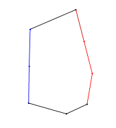
(a) Group edges

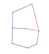
(b) Find sections

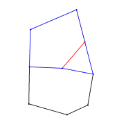
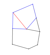
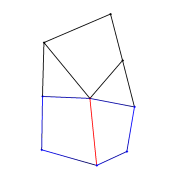
(c) Divide and conquer

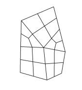
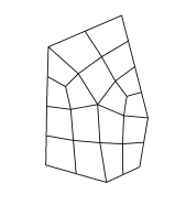
(d) Quads unsmoothed/smoothed

Figure 5: Facet tessellation steps.

2.3 Edge Collapse

Despite its provably excellent properties of convexity with convex planar facets, the Voronoi tessellation may still contain very thin facets (slivers) that can lead to poorly conditioned elements. To eliminate these and to generate a more uniform mesh with a bounded ratio of the longest to the shortest edge, we first perform edge collapse on the Voronoi cells. Any edge shorter than a given tolerance is collapsed, and its two vertices are fused into one. If after edge collapse the number of edges on a facet is $<$ 3, the facet is deleted. Subsequent to edge collapse, we use vertex insertion to ensure that the longest edge is below a certain threshold.

A risk with edge collapse is that facets lose their planarity and, worse, might not face the sphere that they are nominally bounding. We take several steps to avoid this scenario. First, our target edge collapse tolerance of $tol_{\infty}=0.35R$ is not overly aggressive. Second, we make several passes through the data, collapsing the shortest edges first and not allowing a single vertex to be moved more than once per pass, even if it is attached to more than one short edge. With each pass, we set the tolerance to be $tol_{k}=0.35R(0.6)^{8-k}$ for $k=1,\dots,8$, and $tol_{k}=0.35R$ for $k$=9 and 10. As a final precaution, we have the option of revisiting a neighborhood if at the end of the meshing process the algorithm produces hexes with inverted Jacobians. In that case we rerun the algorithm with tighter local tolerances. In the limit of $tol_{\infty}=0$ we recover the provably workable properties of the original Voronoi tessellation. (We find this corrective step necessary only for the ${\cal N}=350$K case.) We remark that many of the challenges in the meshing process come from the domain boundaries, where the Delaunay triangulation has relatively long edges. Consequently we typically set $tol_{\infty}=0.25$ in the neighborhood of $\partial\Omega$.

Another issue with edge collapse is that the reconstructed facet surface will potentially intersect the sphere that is to be bounded by the facet. To avoid this situation, we project all points generated during edge insertion or facet tessellation onto a sphere that is larger than $R_{0}$.

2.4 Vertex Insertion

In addition to having short edges (mostly cleaned by edge collapse), the initial Voronoi decomposition can yield facets with edges that are longer than desired. For this reason we insert vertices for edges that are longer than $0.8R$; thus we have a maximum edge-length ratio of 0.8/0.35. This value is readily adjusted at construction time and is also adjusted somewhat by the final mesh smoothing process. For our initial trials, however, it seems to be a reasonable ratio.

2.5 Facet Tessellation

A major part of the algorithm is the all-quad decomposition of the Voronoi facets. Each facet can be tessellated into a set of quadrilaterals by first inserting a vertex at the midpoint of each edge in order to guarantee that the facet is a polygon with an even number of edges. Alternatively, one can decompose the facet into quads and triangles and perform the midside node insertion at the end. We follow the latter approach.

As illustrated in Fig. 5, our facet tessellation uses a two-phase divide-and-conquer algorithm to reduce the number of vertices on each polygon by splitting facets into smaller polygons. Phase one, illustrated in Fig. 5(a) and (b), begins by clustering sequences of edge vertices having angles $>155^{\circ}$ into edge groups. If the facet is large (having either many vertices or large area), we insert a point at the barycenter. Each edge group having at least one interior vertex angle will connect one and only one vertex to the barycenter. The selected vertex is the one with minimal bias between its adjacent angles (i.e., as close to a bisector as possible). In the case of Fig. 5(b) we see that this process subdivides the facet into two subdomains.

For each subdomain (or for the whole facet if we skip phase one), we consider sequences of 4 successive vertices to see whether they produce viable quads and whether the remaining part of the domain meets quality conditions such as low variance in edge length and absence of large angles. We also consider finding triangles from successive vertex triplets with similar quality metrics. With a slight bias toward quads, the quality indices are compared, and the algorithm chooses the partition that yields the best quality. In the upper subdomain of Fig. 5(c) we see that a triangle is selected that is nearly equilateral. The algorithm is applied recursively, which yields in this case another triangle and a quad in the upper subdomain. Applying the same algorithm to the lower subdomain yields two quads.

From the divide-and-conquer phase, all quads are subdivided into four smaller quads and triangles into three quads, resulting in an initial all-quad tessellation of the facet, shown in Fig. 5(d), left. Laplacian smoothing is applied to this decomposition to yield the final result, shown in Fig. 5(d), right.

We reiterate that, because of edge collapse, the edge points are typically not planar, and points in the facet interior are therefore projected onto the original bisecting plan to avoid ending up in the sphere interiors. The full-mesh smoothing step will accommodate any misshapen elements generated by this projection.

2.6 Sweeping

Once the facets are tessellated, we generate an initial all-hex mesh by projecting each facet-based quadrilateral onto the sphere(s) that are bounded by the facet, or onto the domain boundary. To leave room for an additional thin element layer (“boundary layer”) near the spheres, we take the initial sphere diameter to be $R_{0}=0.8889R$. The sweeping is illustrated in Fig. 2. In this initial phase, however, only one layer of elements is generated so that an initial mesh smoothing may be applied at relatively low element counts.

2.7 Mesh Smoothing

The initial all-hex mesh (comprising 33M elements in the ${\cal N}$=350K case), is smoothed by using a combination of Laplacian smoothing and element-Jacobian optimization following the strategy outlined in  [15, 16]. In addition to the condition-number-based optimization function, we add a substantial penalty term for negative Jacobians. The mesh smoothing thus consists of two parts: Laplacian smoothing and optimization. These are alternated over a sequence of ten passes. Because of the complexity of the objective function, we execute this phase in parallel, using Nek5000 [15]. We describe the basic smoothing steps in the sequel.

2.7.1 Laplacian smoothing

Nek5000 has a highly scalable gather-scatter utility, gslib, which is a stand-alone C library that scales to millions of ranks. It is the workhorse for all interelement operations in Nek5000 because it requires no topological information other than a global ID for each vertex in the graph. (There are 8 such vertices for each hex, each having a unique ID in the global mesh.) The Laplacian smoother is built on gslib’s vector assembly operation, which effects a sum and redistribute of values sharing the same global IDs in the graph. The mathematical expression for this operation is ${\underline{v}}_{L}=QQ^{T}{\tilde{\underline{v}}}_{L}$, where $Q$ is a Boolean matrix that maps (copies) global entities to their local (element-based) counterparts (the FEM scatter operation) [17].

We begin with a shrinking step. For each element, $\Omega^{e}$, we have an isoparametric mapping of the form

$${\bf x}\bigg{|}_{\Omega^{e}}\;=\;{\bf x}^{e}({\bf r}) = \sum_{i=1}^{8}{\bf x}_{i}^{e}l_{i}({\bf r}),$$ (1)

where ${\bf r}\in{\hat{\Omega}}:=[-1,1]^{3}$ and $l_{i}$ is the set of cardinal Lagrange basis functions having nodes at the 8 vertices, ${\bf r}_{i}$, of ${\hat{\Omega}}$. For each element we create a new set of coordinates,

$${\tilde{\bf x}}^{e}_{j} := \sum_{i=1}^{8}{\bf x}_{i}^{e}l_{i}({\tilde{\bf r}_{j}}),$$ (2)

where ${\tilde{\bf r}_{j}}=s{\bf r}_{j}$ and $s=0.95$ is a scale factor. The new coordinates are thus interpolants of ${\bf x}^{e}_{i}$, interior to $\Omega^{e}$. On domain boundaries, we set the corresponding ${\tilde{\bf r}}=(\tilde{r},\tilde{s},\tilde{t})$ to $\pm 1$ as needed, so that the points do not move normal to the domain surface.

Subsequent to this shrinking step, we apply direct stiffness summation [18] (actually, direct stiffness averaging), in which the coordinates of elementwise-shared vertices are added together and divided by the vertex multiplicity (i.e., the number of elements that share that global vertex). We then reproject boundary points to their corresponding boundary surface since the averaging step may potentially move vertices off of curved surfaces. This Laplacian smoothing process is fast, both in serial and in parallel. It can be repeated multiple times for varying values of $s$. We typically apply it about ten times in order to even out the element sizes, particularly on the sphere surfaces.

2.7.2 Optimization smoothing

The second smoothing tool is based on optimization, following the ideas of Knupp [16, 19, 20] and Mittal and Fischer [15]. Unlike Laplacian smoothing, it is more localized and will not tend to redistribute the resolution. It will, however, ensure locally high-quality elements.

We define as an objective function the condition number of the local Jacobian matrix in the Frobenius norm. For each vertex, ${\bf x}_{i}^{e}$, the local Jacobian matrix is

$$\left[J^{e}_{i}\right]_{j,k}=\frac{\partial x_{j}}{\partial r_{k}}\bigg{|}_{{\bf x}={\bf x}^{e}_{i}},$$ (3)

where ${\bf x}=(x_{1},x_{2},x_{3})$ is the physical coordinate and ${\bf r}=(r_{1},r_{2},r_{3})$ is the reference coordinate. The global objective function is the average of local functions,

$$f({\bf{\underline{x}}})=\frac{1}{E}\sum_{e}^{E}{\tilde{\phi}^{e}}=\frac{1}{E}\sum_{e}^{E}\left[\frac{1}{8}\sum_{i}^{8}(\phi_{i}^{e})^{2}\right],$$ (4)

with

$$\phi_{i}^{e}=\frac{1}{3}\left(||J_{i,e}||_{F}||J_{i,e}^{-1}||_{F}\right).$$ (5)

The minimum value of the global objective function is 1, which is realized when the mesh is a 3D cubic lattice.

To repair elements that have a negative Jacobian, we augment ${\tilde{\phi}}^{e}$ with a penalty term,

$$\hat{\phi^{e}}({\bf x}^{e}) = {\tilde{\phi}^{e}}({\bf x}^{e})-\tau\,J_{i}^{e}/J_{max}\cdot\mathbbm{1}_{\{J_{i}^{e}<\epsilon\}}({\bf x}^{e}).\hskip 3.61371pt$$ (6)

We choose $\tau=1000E$, $\epsilon=0.001$, and $J_{max}=\max_{i,e}J_{i}^{e}$.

The optimization is solved by the conjugate gradient method. For each global vertex $i$, the $j$th dimension gradient of the objective function can be computed by

$$g_{j}({\bf x}_{i}) = \sum_{e=1}^{E}\frac{\partial\hat{\phi^{e}}}{\partial x_{j}}\bigg{|}_{{\bf x}_{i}}\;=\;\sum_{e\in{\cal E}(x_{j})}\frac{\partial\hat{\phi^{e}}}{\partial x_{j}}\bigg{|}_{{\bf x}_{i}},$$ (7)

where ${\cal E}({\bf x}_{i})$ is a set of elements sharing the vertex ${\bf x}_{i}$. The last sum can be assembled by $Q^{T}$, the gather (i.e., direct-stiffness summation) operation in the FEM, such that ${\underline{g}}=Q^{T}{\underline{g}}_{L}$. This framework allows us to compute the gradient locally, element-by-element, and to then gather all local gradients at once.

We approximate the local gradient with a central difference approximation along the unit vector ${\bf e}_{j}$ in the $j$th dimension,

$$g^{e}_{i,j} \approx \frac{1}{2h}\left[\hat{\phi^{e}}({\bf x}_{i}+h{\bf e}_{j})-\hat{\phi^{e}}({\bf x}_{i}-h{\bf e}_{j})\right],$$ (8)

where the step size $h$ is chosen to be $0.001$ times the shortest edge.

We remark that for large element counts (e.g., $E=10^{5}$–$10^{8}$), our Matlab version of optimization is slow because it is difficult to avoid for loops. We thus execute the mesh smoothing in Nek5000 since these routines are already available there [15]. Since the quality of the initial mesh coming from the Voronoi-based scheme is already high, we do not have difficulty with mesh tangling. Nonetheless, this is one area where our algorithm could be improved by using, for example, edge-oriented algorithms such as presented in [21, 22].

2.7.3 Boundary smoothing

The mesh smoothing or optimization is constrained by the boundary condition. For improved mesh quality, we allow the boundary vertices to slide along the boundary surfaces. As mentioned earlier, for Laplacian smoothing, the direction toward the boundary face will not be shrunk, and points are reprojected onto the surface after the averaging operator.

As for the optimizer, the full objective function should include a Lagrange multiplier that would add a penalty for boundary points moving away from boundary. In fact, the gradient of the boundary constraints are in the same direction of the normal vector of the boundary surface. Therefore, we decompose the gradient at the boundary into normal and tangential components and have to eliminate the movement only along the normal direction,

$$\hat{{\underline{g}}}_{e,i}\big{|}_{\partial\Omega} = {\underline{g}}_{e,i}\big{|}_{\partial\Omega}-{\underline{g}}_{e,i}\big{|}_{\partial\Omega}\cdot{{\hat{\bf n}}}.$$ (9)

To make sure the boundary points are still attaching on the boundary surface after all of the movement, we apply the orthogonal projection at each iteration.

2.8 Mesh refinement

The mesh smoothing will produce a valid mesh. At this stage, in each cell, there is only one layer of elements between facet and sphere. In order to meet the requirement for the fluid simulations, the mesh needs to be refined.

2.8.1 Cell refinement

In each cell, we can arbitrarily refine the element in the radial direction of the sphere without breaking the conformality between other cells. Here, we add a midlayer by splitting the elements into two in the radial direction. To gradually increase the resolution near spheres, we split the elements in a ratio of 55% (near facet) versus 45% (near sphere). This action effectively doubles the number of elements.

2.8.2 Extrusion

Extrusion is used to generate extra layers of elements for CFD computations. We typically generate one extra layer inward to the spheres to resolve the boundary-layer of the fluid solution near the sphere walls. Similarly, we add an extra layer outward on the cylinder wall. In the flow direction we extrude three layers toward the bottom of the domain (the flow inlet) and seven layers for the outflow region on the top. The single-layer extrusion on the spheres increases the total number of elements by an additional $1.5\times$ after the first refinement. As seen in Fig. 2, the resulting mesh has three layers between the facet and sphere. For polynomial degree $N=7$, this yields about 42 points between adjacent spheres, which is sufficient for large-eddy simulation at the target Reynolds numbers based on the hydraulic diameter.

2.9 Projection

The final step of the meshing process is to project the facet quadrilaterals that tessellate the sphere and boundary surfaces onto their actual locations. This step is done inside Nek5000 because it requires projection of the full set of GLL points onto the target geometry. Typically, we perform this step in two passes. First, we project at low-order ($N=2$) in order to generate a hex27 mesh description that can be used as a starting point for Nek5000. In this phase, we also inflate the sphere surfaces to the target radius, $r<R$. Flat spots are included to enforce a prescribed gap that avoids contact singularities using the projection algorithm illustrated in Fig. 6.

Figure 6: Enforcement of a gap between Sphere 0 and 1. Any point on the surface of Sphere 0 that is nominally projected to ${\bf p}$ is shortened so that its projected component onto ${\bf x}_{0}$–${\bf x}_{1}$ is equal to $\hat{\bf p}$.

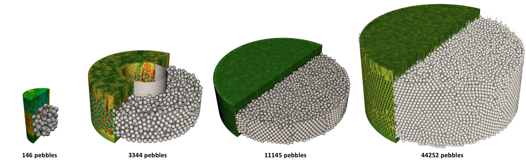
Figure 7: Pebble meshes and simulations.

Statistics for Several Multisphere Configurations
Case	${\cal N}$	Source	Container	$E$	$E/{\cal N}$
cyl146	146	Experiment	cylinder	62,132	425.56
box1053	1,053	StarCCM+	box	376,828	250.72
cyl1568	1,568	StarCCM+	cylinder	524,386	334.43
cyl3260	3,260	StarCCM+	cylinder	1,121,214	343.93
ann3344	3,344	Project Chrono	annulus	1,133,446	338.95
cyl11k	11,145	Project Chrono	cylinder	3,575,076	320.78
cyl44k	44,257	Project Chrono	cylinder	13,032,440	294.47
cyl49k	49,967	Project Chrono	cylinder	14,864,766	297.49
ann127k	127,602	StarCCM+	annulus	39,249,190	307.52
ann350k	352,625	StarCCM+	annulus	98,782,067	280.13

Table 1: List of cases meshed to date including the number of spheres ${\cal N}$, the data source, domain shape, number of elements $E$, and number of elements per sphere.

Meshing Time Breakdown (sec)
Meshing Step	cyl146	cyl1568	ann3344	cyl11k	cyl49k	ann127k	ann350k
IO for Qhull	4.56E-01	1.10E+00	2.64E+00	6.36E+00	1.97E+01	5.13E+01	2.79E+02
Voronoi cells (Qhull)	1.70E-01	4.29E-01	1.07E+00	2.50E+00	8.77E+00	2.12E+01	7.98E+01
Facet generation	1.66E-01	1.51R+00	4.22E+00	1.90E+01	1.77E+02	9.14E+02	4.20E+03
Edge collapse	8.67E-02	2.34E-01	4.53E-01	1.26E+00	5.24E+00	1.30E+01	8.20E+01
Facet/edge clean-up	1.21E+00	6.57E+00	8.66E+00	2.75E+01	1.29E+02	3.47E+02	2.55E+03
Tessellation	1.43E+00	9.76E+00	1.87E+01	6.26E+01	2.84E+02	6.70E+02	1.65E+03
All-quad generation	1.67E-01	7.02E-01	1.34E+00	4.24E+00	1.74E+01	4.61E+01	1.20E+02
All-quad to all-hex	5.64E-02	2.48E-01	5.13E-01	2.42E+00	9.34E+00	2.52E+01	7.97E+01
Extrusion 1	4.99E-01	3.58E+00	8.60E+00	2.11E+01	8.58E+01	3.10E+02	1.63E+03
IO for smoothing	2.42e-01	4.99E+00	4.13E+00	1.30E+01	5.85E+01	1.96E+02	1.12E+03
Mesh smoothing	3.58e+00	4.12E+01	9.95E+01	3.99E+02	7.26E+02	3.19E+03	1.10E+03
(nodes, $N$)	(1, $N$=1)	(1, $N$=1)	(1, $N$=1)	(2, $N$=1)	(4, $N$=1)	(8, $N$=1)	(24, $N$=1)
Extrusion 2	1.01E+00	5.36E+00	1.08E+01	2.80E+01	1.10E+02	6.72E+02	2.12E+03
IO for projection	1.55E-01	7.71E-01	1.62E+00	5.13E+00	2.19E+01	1.62E+02	4.16E+02
Curve-side projection	4.00E+01	2.10E+02	1.80E+03	1.68E+03	4.20E+03	3.60E+03	7.20E+03
(nodes, $N$)	(1, $N$=2)	(1, $N$=2)	(1, $N$=2)	(2, $N$=2)	(4, $N$=2)	(8, $N$=2)	(600, $N$=7)
Total	6.53E+01	2.70E+02	1.91E+03	2.04E+03	4.27E+03	1.09E+03	5.10E+04

Table 2: Timing breakdown of meshing measured in seconds. Most steps are performed in serial using Matlab on a workstation (Intel Xeon E5-2630 v3 @2.40GHz) while the ones performed in parallel are provided with the number of nodes and the polynomial order $N$. The smoothing and projection are performed on OLCF/Summit using 42 cores per node. Note that the case of ann350k required two passes through the entire procedure to adjust the edge-collapse tolerance.

Figure 8: Turbulent flow in an annular packed bed with ${\cal N}=352625$ spheres meshed with $E=98,782,067$ spectral elements of order $N=8$ ($n=50$ billion gridpoints). This NekRS simulation requires 0.233 seconds per step using 27648 V100s on Summit. The average number of pressure iterations per step is 6.

Nek5000 performance comparison between hex and tet-to-hex meshes for 146 pebbles
Mesh	Node	Core	$E$	$E$/core	$N$	$n$	$n$/core	$v_{i}$	$p_{i}$	CFL	$t_{step}$	R
all-hex	16	672	62132	92	7	21311276	3.1713e+04	2.0	5	0.92	0.2954	1
tet-to-hex	16	672	365844	544	4	23414016	3.4842e+04	1.1	17	2.11	0.9251	3.13

Table 3: Nek5000 performance comparison of all-hex and tet-to-hex on Summit (CPU) for ${\cal N}=146$ with $Re=5000$. Simulations were performed for 200 steps with step size $\Delta t$=8.00E-04. Per-step averages are taken over the last 100 steps. Here, $v_{i}$ and $p_{i}$ represent respective average velocity and pressure iteration counts, and $t_{step}$ is the average wall clock time, in seconds. $R$ represents the ratio of all-hex to tet-to-hex for $t_{step}$. Characteristic-based BDF2 with 2 substeps is used for timestepping and overlapping-Schwarz smoothing with spectral element multigrid preconditioning with HYPRE AMG for coarse-grid solve is used for pressure solve. Tolerances for pressure and velocity are $10^{-4}$ and $10^{-6}$, respectively.

Figure 9: Nek5000 simulation wall time per timestep and pressure iterations for the case of Table 3.

Figure 10: Prototype mesh for contacting spheres. Cut-away view on the left.

3 Results

We have applied the algorithm described in Section 2 to the configurations listed in Table 1. The number of elements per sphere for the three-layer configuration yields $\approx$300 elements per sphere, including the elements in the inlet- and exit-flow regions. Figure 7 shows several of the corresponding sphere configurations along with axial-flow velocity distributions. Regions of order and disorder are evident in the positions of the spheres along the domain wall for the case ${\cal N}=44252$. Such ordered packing has a direct influence on the flow conditions near the domain boundary and is an important consideration for thermal-hydraulics analysis. All of the cases shown here were run with NekRS (the GPU-oriented version of Nek5000) using the NVIDIA V100s on OLCF’s Summit at Oak Ridge National Laboratory.

Table 2 provides a timing breakdown (in seconds) for the signicant components of the mesher, across the full spectrum of problems ranging from 62K elements for ${\cal N}$=146 to 99M elements for ${\cal N}$=352K. Only the 352K case needs to be iterated because of a handful of bad Jacobians in the mesh using the original edge-collapse tolerance. This iteration likely could be avoided with improved smoothing algorithms. For similar reasons, we perform the final projection and smoothing for the 352K case for the $N=7$ (512 points per hex) configuration, rather than the standard hex27 used for the other meshes. We note that the facet generation and tessellation are bottlenecks because of unavoidable for loops in the (interpretive-based) Matlab code. Rewriting these as $C$-based Mex files would likely alleviate this bottleneck.

Regarding mesh optimization, we recall that initial smoothing is applied before refinement, which means that it is applied to only $\approx 33$M elements for the ${\cal N}=352$K case of Fig. 8. With 10 outer smoothing passes, each using 3 Laplacian smoothings followed by 120 optimization steps (requiring 1100 seconds on 1,008 CPU cores of Summit), we find signifcant improvements:
Before optimization:

• 369 elements with negative Jacobians
  

• min scaled Jacobian = -5.94
  

• max aspect ratio = 3.63e4
  

• node spacing: (min, max) = (2.32e-5, 7.49e-1)
  

After optimization:

• Valid mesh—all Jacobians positive.
  

• min scaled Jacobian = 1.93e-2
  

• max aspect ratio = 3.08e1
  

• node spacing: (min, max) = (4.27e-2, 8.71e-1)
  

In Table 3 and Fig. 9 we compare the performance of the all-hex meshing strategy with the tet-to-hex approach [8] for the ${\cal N}=146$ case. At comparable resolution $n$, the all-hex approach has a lower Courant number (CFL) for the same timestep size and a lower wall-clock time per timestep because of the reduction in pressure iteration counts. The lower CFL implies that the all-hex approach could use a larger timestep, thereby further reducing simulation costs.

4 Conclusion and Future Developments

We have presented an approach to construction of high-quality all-hex meshes for the interstitial space in dense-packed spheres at relatively low element counts. The algorithm uses an $O({\cal N})$-complexity Voronoi decomposition to decouple the problem into local problems that can be meshed independently. Sliver removal, vertex insertion, automated facet tessellation, and mesh smoothing are all critical components for generating production-quality meshes. All issues regarding boundary conditions and projection of the final GLL nodal points for the SEM onto the sphere are addressed. The success of the algorithm is demonstrated over a broad range of mesh sizes, from ${\cal N}=146$ to 352K, with the largest case corresponding to $E=99$ million spectral elements and $n=50.5$ billion grid points.

Overall, the development has satisfied the objective of allowing us to produce large-scale high-quality meshes suitable for high-order spectral element simulations of turbulence in packed beds. In particular, the 352K case, which corresponds to a full reactor core, takes only 0.233 seconds per step when running on 4,608 nodes (27,648 V100s), which corresponds to 1.8 million points per V100. This configuration would require only 6 hours to compute a single flow-through time on all of Summit, implying that parameter studies will be readily tractable on exascale platforms. The number of pressure iterations is $\approx$6 per step when using a tuned version of the NekRS multigrid solver. Tuning was required because the highly compressed elements that are squeezed between the nominal sphere contact points lead to ill-conditioning of the Poisson problem.

A future development for our mesher will be to replace the flattened spheres at the contact points with a chamfered bridge of solid material that will join the spheres and bypass the point-contact singularity, as illustrated in Fig. 10. Preliminary experience suggests that elimination of the narrow gap leads to a significant reduction in the condition number of the discrete pressure-Poisson operator and should further improve runtimes.

The submitted manuscript has been created by UChicago Argonne, LLC, Operator of Argonne National Laboratory (“Argonne”). Argonne, a U.S. Department of Energy Office of Science laboratory, is operated under Contract No. DE-AC02-06CH11357. The U.S. Government retains for itself, and others acting on its behalf, a paid-up nonexclusive, irrevocable worldwide license in said article to reproduce, prepare derivative works, distribute copies to the public, and perform publicly and display publicly, by or on behalf of the Government. The Department of Energy will provide public access to these results of federally sponsored research in accordance with the DOE Public Access Plan. http://energy.gov/downloads/doe-public-access-plan

References

- [1] Kolev N. Packed bed columns: for absorption, desorption, rectification and direct heat transfer. Elsevier, 2006
- [2] Merzari E., Yuan H., Min M., Shaver D., Rahaman R., Shriwise P., Romano P., Talamo A., Lan Y., Gaston D., Martineau R., Fischer P., Hassan Y. “Cardinal: A lower length-scale multiphysics simulator for pebble bed reactors.” Nucl. Tech., American Nuclear Society, 2020
- [3] Patera A. “A spectral element method for fluid dynamics : laminar flow in a channel expansion.” J. Comp. Phys., vol. 54, 468–488, 1984
- [4] Stephenson M.B., Canann S.A., Blacker T.D. “Plastering: a new approach to automated, 3D hexahedral mesh generation–Progress Report I.” Tech. Rep. 89-2192, Sandia National Labs., Albuquerque, 1992
- [5] Cass R., Benzley S., Meyers R., Blacker T. “Generalized 3-D paving: an automated quadrilateral surface mesh generation algorithm.” Int. J. for Num. Meth. in Eng., vol. 39, no. 9, 1475–1489, 1996
- [6] Leland R., Melander D., Meyers R., Mitchell S., Tautges T. “The Geode Algorithm: Combining Hex/Tet Plastering, Dicing and Transition Elements for Automatic, All-Hex Mesh Generation.” IMR, pp. 515–521. 1998
- [7] McDill J., Carmona Garcia A. “Tet-to-Hex Conversion for Finite Element Analysis.” AIP Conference Proceedings, vol. 712, pp. 2210–2215. American Institute of Physics, 2004
- [8] Yuan H., Yildiz M., Merzari E., Yu Y., Obabko A., Botha G., Busco G., Hassan Y., Nguyen D. “Spectral element applications in complex nuclear reactor geometries: Tet-to-hex meshing.” Nuclear Engineering and Design, vol. 357, 110422, 2020
- [9] Fischer P., Min M., Rathnayake T., Dutta S., Kolev T., Dobrev V., Camier J., Kronbichler M., Warburton T., Swirydowicz K., Brown J. “Scalability of High-Performance PDE Solvers.” IJHPCA, vol. 34, 5, 562–586, 2020
- [10] Cruz M.E., Patera A.T. “A parallel Monte Carlo finite-element procedure for the analyis of multicomponent random media.” J. Num. Meth. Eng., vol. 38, 1087–1121, 1995
- [11] Cruz M.E., Ghaddar C.K., Patera A.T. “A variational-bound nip-element method for geometrically stiff problems; application to thermal composites and porous media.” Proc: Math. Phys. Sci, vol. 449, 93–122, 1995
- [12] Sheffer A., Etzion M., Rappoport A., Bercovier M. “Hexahedral Mesh Generation using the Embedded Voronoi Graph.” Engineering with Computers, vol. 15, no. 3, 248–262, 1999
- [13] Yan D.M., Wang W., Lévy B., Liu Y. “Efficient Computation of 3D Clipped Voronoi Diagram.” pp. 269–282, 2010
- [14] Nguyen T., Kappes E., King S., Hassan Y., Ugaz V. “Time-resolved PIV measurements in a low-aspect ratio facility of randomly packed spheres and flow analysis using modal decomposition.” Experiments in Fluids, vol. 59, no. 8, 1–29, 2018
- [15] Mittal K., Fischer P. “Mesh Smoothing for the Spectral Element Method.” J. Sci. Comput., vol. 78, no. 2, 1152–1173, 2019
- [16] Knupp P. “Introducing the target-matrix paradigm for mesh optimization via node-movement.” Engineering with Computers, vol. 28, no. 4, 419–429, 2012
- [17] Deville M., Fischer P., Mund E. High-order methods for incompressible fluid flow. Cambridge University Press, Cambridge, 2002
- [18] Strang G., Fix G. An Analysis of the Finite Element Method. Prentice-Hall Series in Automatic Computation. Prentice-Hall, Englewood Cliffs, NJ, 1973
- [19] Knupp P.M. “Hexahedral Mesh Untangling & Algebraic Mesh Quality Metrics.” IMR, pp. 173–183. Citeseer, 2000
- [20] Knupp P.M. “A method for hexahedral mesh shape optimization.” Int. J. Num. Meth. in Eng., vol. 58, no. 2, 319–332, 2003
- [21] Livesu M., Sheffer A., Vining N., Tarini M. “Practical hex-mesh optimization via edge-cone rectification.” ACM Transactions on Graphics (TOG), vol. 34, no. 4, 1–11, 2015
- [22] Xu K., Gao X., Chen G. “Hexahedral mesh quality improvement via edge-angle optimization.” Computers & Graphics, vol. 70, 17–27, 2018